


Highlights
What are the main findings?
- A cell-wise output with one self-slot and two unordered connection slots turns satellite imagery directly into lane marking polylines and reaches an AI-CCQ F1 of 0.4483 on the SEED-MAP test set.
- Supervising only the connection direction is better than regressing the displacement, and injecting the ground truth shows that the representation and the decoder lose little information (F1 of 0.95).
- The proposed AI-CCQ metric scores each lane marking as one instance. It accepts partly drawn lines and rejects lines that switch to a neighboring marking.
What are the implications of the main findings?
- Lane markings that meet or cross are separated into individual instances much more reliably than with segmentation.
- The detected polylines can serve as draft lane marking candidates for producing and updating HD maps.
Abstract
High-definition (HD) maps for autonomous driving store each lane marking as a separate polyline. Satellite imagery covers wide areas at low cost, but current methods cannot turn it directly into such polylines. The reason is that no existing output representation suits polyline detection. Segmentation masks do not tell which line a pixel belongs to, and they merge lines that meet or cross. Existing cell-wise connectivity representations tie their output slots to fixed angular sectors. Their training target therefore changes discontinuously at sector boundaries. We propose STELLA, an output representation suited to polylines, and a method to train it. At each grid cell, STELLA predicts one self-slot and two unordered connection slots. During training, these slots are matched to the ground-truth (GT) connections at minimum cost. One line thus becomes one chain of cells, and post-processing only cleans up overlapping lines. We also propose AI-CCQ, an asymmetric instance-level metric for thin, long lines. It gives credit to a partly drawn line but rejects a line that switches to a neighboring marking. On the SEED-MAP test set, STELLA reaches an AI-CCQ F1 score of 0.4483, against 0.3005 for a segmentation-based method and 0.3551 for the Sat2Graph representation.
1. Introduction
HD maps help an autonomous vehicle locate itself and compute the lanes it can drive in. Lane markings are a core element of these maps. A map must store each lane marking as a separate polyline instance, not as a group of pixels. The next steps of map production, map matching and lane topology computation, need line geometry.
Most HD maps have been built with mobile mapping systems (MMSs). A survey vehicle drives on the road and records the surface with its sensors. The production cost therefore grows with the total road length. When a road changes, the vehicle has to drive that section again, so the update cycle is long. Satellite imagery has a different cost structure. One acquisition covers hundreds of square kilometers at once. The image already has geographic coordinates when it is taken, so it is simple to combine with existing map systems.
Two developments have made this approach possible only recently. First, the optical resolution of commercial satellites now lets a person tell road markings apart by eye. Second, public datasets that annotate each lane marking as a separate line have appeared since 2024. Earlier aerial datasets annotated lane centerlines or lane pixels, not individual lane markings.
However, detecting lane markings as individual lines from satellite imagery is still difficult for five reasons. First, the target is a thin intensity structure, not an object. At a ground sample distance (GSD) of 0.255 m/px, a paint line 0.15 m wide [1] is narrower than one pixel [2]. It appears as a thin, elongated structure that is slightly brighter than its surroundings and has no clear boundary. Second, connectivity cannot be decided from local information. Shadows, occlusion by trees and vehicles, worn paint, and dashed patterns break a marking into pieces [3]. The pixels at one location cannot tell whether two pieces belong to the same line [4]. Third, lines cross one another at intersections. In a pixel mask, the crossing lines form a single tangled region [5], and the mask does not record which line continues into which [6]. The output representation itself therefore needs to carry connection information. Fourth, the output must be a set of polylines, not pixel areas [7,8]. Fifth, the lines are dense. A 768 × 768 px tile contains 38.3 line instances on average in the training data, and up to 255. A representation with a fixed number of output queries [9,10] must be sized for the densest tile.
Representations for lane detection in ground-level images assume a vehicle on the road that looks forward. Row-wise classification [11], anchors that start from the image border [12], and a fixed number of lanes all come from this assumption. The assumption does not hold for a satellite tile. Lines can run in any direction and can start and end inside the image.
Query-based vectorized map construction assigns instances to a fixed number of queries [7,10,13]. The densest tiles hold up to 255 instances, about five times the 50 queries used by MapTR and MapTRv2 [10,13].
Methods that combine segmentation with post-processing are good at labeling paint pixels. However, they cannot separate lines that meet or cross. Skeletonization creates branches at crossing points. Connected-component analysis groups all overlapping lines into one component. Watershed [2] has no basis to decide which line a seed belongs to. Separating and joining lines is therefore left entirely to post-processing. When the painted region is briefly interrupted, the line is also cut at that point.
Evaluation is a second open problem, because no existing metric measures what map production needs from thin, long lines. Pixel-based metrics do not check whether a line is predicted in one piece. Instance metrics with strict matching give zero credit to every fragmented prediction. Both kinds of metrics also weigh all geometric errors equally. In map production, however, an incomplete line is much cheaper to correct than a misplaced one. We therefore propose the asymmetric instance-level completeness, correctness, and quality metric (AI-CCQ). It evaluates together how much of each line is covered, whether each line is predicted as one continuous instance, and how little manual editing the prediction needs before it can go into the map.
This paper proposes STELLA (Satellite Topology Estimation for Lane-Level Analysis), a lane marking detection method for satellite imagery that is built on a new output representation. With this representation, the network outputs each lane marking as a separate polyline with a class, and only light post-processing is needed. At each grid cell, STELLA predicts one self-slot and two connection slots. The self-slot gives the class of the line and its position inside the cell. A connection slot gives a direction in which the line continues from the cell. The two connection slots have no order. The decoder links slots that face each other into chains, and each chain becomes one polyline. Figure 1 shows the polylines that STELLA detects in four scenes. The ground truth (GT) is encoded in the same format. The GT and the output therefore share the same grid, the same fields, and the same number of slots. The only remaining difference between them is the order of the slots.
Figure 1.
Examples of detected lane markings. Polylines from four different scenes are drawn in class colors. Both endpoints of each polyline are marked with a white-rimmed circle. The legend below the images gives the color of each class. All later figures use the same class colors and endpoint circles. The top two scenes are intersections. The bottom two scenes are straight arterial roads along a river and through a city.
This paper makes four contributions. First, it proposes a novel output representation for extracting lane markings from images, together with a training method suited to it. Each cell outputs its connections to the neighboring cells of the same line. Polylines can therefore be recovered with minimal post-processing. Second, it proposes a network that builds a separate token for each slot. The three tokens of a cell are separated from the input of the attention layers, not only at the output layer. The two connection slots must point in opposite directions, and this design lets each of them learn its own role. Third, it proposes a polyline recovery algorithm designed for this representation. The algorithm grows each chain by linking connection slots that face each other, and it has no learned parameters. The algorithm can skip a cell that is lost at a crossing or under an occlusion and continue the same chain. Fourth, it proposes a new asymmetric instance metric for thin, long lines. We call this metric AI-CCQ. Unlike pixel-based metrics, it checks whether each line is predicted as one instance. Unlike strict instance matching, it still gives credit to a line that is cut once, as long as one piece covers most of it. Its strict correctness threshold rejects lines that switch to a neighboring lane marking, which are the most costly errors for a human map editor.
STELLA is not meant to replace surveying. Its role is to generate lane marking candidates automatically for map production and updating.
2. Related Work
2.1. Lane Detection in Ground-Level Images
Lane detection in ground-level images has developed along four lines. Segmentation-based methods predict lane pixels and then group them into lines by clustering [14]. Anchor-based and parametric methods represent a lane as a line anchor or as the coefficients of a low-order curve [12,15,16]. Keypoint-based methods predict points on a lane and connect them [17,18]. Sequential methods generate a lane as a sequence of tokens [19]. All four lines of work assume a vehicle on the road that looks forward. This assumption does not hold for a satellite tile.
2.2. Query-Based Vectorized Map Construction
Methods that build a vectorized map around a vehicle assign map elements to a set of learnable queries [7,10,13]. In this line of work, the permutation-equivalent modeling of MapTR [10] is the closest prior work to our unordered slots. The two approaches differ in two ways. MapTR treats the order of the points within one instance as an equivalence class. We treat the assignment of the directions that leave one cell as an equivalence class. In addition, a query-based representation must fit the number of instances to its query budget.
2.3. Road Graph Extraction from Remote Sensing Imagery
Road graph extraction from satellite imagery is the closest field to this paper. Early methods derived the graph from segmentation results by post-processing [20,21]. Later, iterative methods traced a road by predicting the next point from the current one [4,22,23]. Recent methods generate the whole graph in a single forward pass [5,24,25].
The graph-tensor encoding (GTE) of Sat2Graph [5] belongs to the same family as our representation. At each grid cell, it predicts a node probability and several edge channels. Each channel describes one edge that leaves the cell. We treat Sat2Graph as the closest prior work and differ from it in four ways.
First, the slot assignment rule is different. Sat2Graph fixes its output channels to angular sectors of 60°. When a direction crosses a sector boundary, the same geometry becomes the target of a different output channel. The training target therefore changes discontinuously. We give the slots no order and match them at each cell with the minimum cost. The loss is therefore invariant to permutations of the slots.
Second, the connection target is different. Sat2Graph regresses the displacement to the neighboring node. This target mixes direction and distance. We supervise only the direction and recover the distance during decoding.
Third, the consistency of the GT encoding is different. The authors of Sat2Graph point out that one graph has many valid encodings, because the vertices on a long road segment can be interpolated in many ways. The GT labels are therefore inconsistent along long segments, and they compute the edge losses only at GT vertices to cope with this. Our encoding places nodes only in the cells that a line actually occupies, and it leaves the two end cells empty. The GT is therefore a deterministic function of the polyline.
Fourth, the output is different. The output of Sat2Graph is one global road graph without classes. Our output is a set of separate polyline instances, each with a class.
2.4. Lane-Level Mapping from Aerial and Satellite Imagery
Work that handles lanes as separate instances in aerial and satellite imagery has started only recently. Several large-scale public datasets with lane annotations have been released [2,26]. Proposed methods include pipelines that vectorize segmentation results and methods that predict vertices and refine them in stages [6,26]. The SEED-MAP dataset used in this paper is one of these datasets [27]. It annotates each lane marking as a separate polyline instance, so instance-level evaluation is possible. Table 1 summarizes the existing representations. Sat2Graph and SAM-Road output one global road graph, so they keep no instance identity. Each of the six slots of Sat2Graph holds an edgeness score and a displacement. STELLA obtains instance identity from its chains.
Table 1.
Comparison of existing methods and their representations.
3. Model
This section describes three parts in order: the output of the model (Section 3.1), the network that produces this output (Section 3.2), and the loss that trains it (Section 3.3). Section 4 describes how the output is converted back into polylines.
3.1. Output Representation
We divide the input tile into cells of 4 × 4 px. A finer grid makes the number of tokens grow quickly. A coarser grid can place two lane markings in one cell, and one cell would then have to represent two lines at once. The measured median distance between neighboring lane markings is about 12 px. With 4 px cells, two neighboring lane markings are therefore about three cells apart.
At each cell, the model predicts a heatmap value, one self-slot, and two connection slots. Table 2 lists their fields, and Figure 2 shows them along one line. The heatmap tells whether a line passes through the cell. The cells that it marks are the body cells in Figure 2. The self-slot gives three quantities, the class, coord, and end fields of Table 2. The class field is the class of the line. The coord field is the position of the line inside the cell, measured from the top-left corner of the cell. This position is the self-point, drawn as a black dot in Figure 2. It describes the line more finely than the 4 px grid. The end field tells whether the cell is the end of a chain.
Table 2.
Output format of the model.
Figure 2.
Cell outputs and a chain. The figure enlarges one part of the grid. A self-point is placed in every body cell that the line passes through. The two connection slots of the highlighted cell point to the previous and the next neighbor. The two end cells are left empty. The line is extended along the outward slot of the cell next to each end cell.
A connection slot gives a direction in which the line continues from the cell. Each cell has R = 2 connection slots. Each slot predicts an existence probability and a unit direction, the exist and dir fields of Table 2. The direction starts at the self-point of the cell. A line is a one-dimensional curve, so it continues in only two directions from any point. In the highlighted cell of Figure 2, slot A points to the previous neighbor and slot B points to the next one. Linking these directions from cell to cell turns one line into one chain of cells.
A connection slot does not store distance. At a crossing, another line may take ownership of a cell. An occlusion may also cause the next node to be skipped. In both cases, the direction in which the line continues stays the same. The training target is therefore not affected by these events. The decoder recovers the actual distance by finding the neighboring node.
The connection slots have no order. We do not decide which of the two slots comes first. A lane marking has no direction of travel. The end from which an annotator drew a line is also not visible in the image. If the slots were fixed to the annotation order, the whole target would flip for a line drawn in the opposite direction. If the slots were assigned to angular sectors, the target would move to a different slot at a sector boundary. Instead, we treat the two slots as a set. At each cell, we match the two predictions to the two GT branches with the best pairing and then apply the loss.
The two end cells of the cell sequence of a line produce no output. A basic limit of a grid representation is that one cell can represent only one line. Most places where lane markings actually overlap are where the end of one line touches the body of another line. If the end cells are left empty, the question of which line owns such a cell does not arise. The decoder only extends the line along the outward slot of the cell next to each empty end cell, the dashed arrows in Figure 2.
The GT is built in the same form. Each line is rasterized separately, and the number of its pixels in each cell is counted. When two lines pass through one cell, the line with more pixels owns the cell. The two directions are then filled along the chain, and the two end cells are left empty. The resulting GT is a deterministic function of the polyline. The same GT is produced regardless of the end from which the line was drawn or the spacing of its points. Two lines of the same class compete for many cells only where they run almost parallel less than one cell apart. Such stretches make up 0.99% (validation) and 1.58% (test) of the total GT length.
The final output is a set of polylines with classes, and it is extracted from this grid output (Section 4). We do not ask the network to predict whole polylines directly. Polylines differ in length, and one tile contains up to hundreds of them. On the grid, each cell predicts only where its line continues, so the output is a tensor of fixed size. This size does not limit the number or the length of the lines.
3.2. Network Architecture
The feature extractor is standard, and the token construction is our own design. Figure 3 shows the whole network.
Figure 3.
Network architecture. Nodes are selected from the grid features. Three role embeddings u0, u1, and u2 are added (⊕) to the grid feature z of a node to form three tokens. The three tokens pass through six attention layers together. On the right, the dot shows the class, the position, and the end state of the cell. The red and green arrows show the existence and the direction of the two connection slots. The orange cells are the cells selected by the heatmap threshold.
Backbone and neck. The image first passes through the standard part on the left of Figure 3, a pretrained convolutional backbone, ConvNeXtV2-L [28]. A light feature pyramid network (FPN) [29] merges the multi-scale features into one grid feature map. The choice of backbone is not a contribution of this paper. Section 6.5 reports how the results change with the backbone.
Node selection. At each cell, the heatmap head in Figure 3 predicts the probability h that a line passes through the cell. The cells with h > τh and their eight neighbors are selected as nodes, where τh is a threshold. We selected it on the validation set and set it to 0.3. Only the selected cells become tokens. During training, we add the cells that the model wrongly predicts as positive to the GT positive cells. The model thus also learns that these cells contain nothing. Only a small fraction of the grid becomes tokens. This sparsity is what makes the architecture feasible.
Three tokens per cell. For each selected cell, we add three learned role embeddings u0, u1, and u2 to its grid feature z. This gives three tokens, one for the self-slot and two for the connection slots. These are the slot tokens in Figure 3. The three role embeddings are shared by all cells. Each embedding therefore tells a token which role it plays. The three tokens of a cell start from the same feature and differ only in their role embeddings. While passing through the attention layers, each token attends to different neighbors and learns its own role.
Attention stack. The attention block in Figure 3 has six layers, and each layer has three parts. First, slot self-attention lets the three tokens of a node attend to one another. Second, neighbor cross-attention lets each token attend to the grid features of other nodes. Third, a feed-forward network (FFN) follows. The range of the neighbor cross-attention depends on the layer. In the first layer, it attends to all nodes in the tile. In the other five layers, it attends only to the nodes inside a 7 × 7 cell window. Section 6.5 shows that a 9 × 9 window gives almost the same F1 and a 5 × 5 window a slightly lower one. The neighbor cross-attention is necessary because connectivity cannot be decided from the pixels of one cell. Position information is given by a two-dimensional rotary position embedding (RoPE) [30,31].
Output heads. The heads on the right of Figure 3 produce the outputs of Table 2. A node has two kinds of outputs, so two heads are enough. The self-head reads the self-token and predicts the class, the in-cell offset, and the end probability. The connection head reads each connection token and predicts an existence probability and a direction. The two connection tokens share this head. A separate head for each slot would give the slots an order, which breaks the unordered design of Section 3.1. The two tokens still give different outputs, because they start with different role embeddings. While passing through the attention layers, they learn to point in nearly opposite directions.
3.3. Loss Functions
The model has six outputs, the six fields of Table 2. The loss therefore has six terms, one for each field, and the terms are summed. Five of the terms use standard forms. For these, we give only the field that each term trains and the form of the loss.
The node loss trains the heatmap field, the probability h of Section 3.2. Positive cells are only a few percent of all cells. We therefore use a focal binary cross-entropy loss [32] to reduce the contribution of easy background cells. The loss is normalized by the number of positive cells.
Three terms train the fields of the self-slot. The class loss trains the class field with a cross-entropy loss at every selected cell. A selected cell that is not in the GT is supervised with the background class. The offset loss trains the coord field with a smooth L1 loss at GT cells only. The end loss trains the end field with a binary cross-entropy loss.
Two terms train the fields of the connection slots. The existence loss trains the exist field with a binary cross-entropy loss. Its target is 1 for a slot that receives a GT branch in the slot matching below, and 0 otherwise. The direction loss trains the dir field. This term is our own, and it is defined below, after the slot matching that it needs.
Slot matching. The slots have no order. Before the loss is applied, we must decide which prediction is compared with which GT branch. We define a cost between a slot and a GT branch of a cell from the direction mismatch and the existence confidence. At each cell, we choose the permutation with the smallest total cost,
where is the unit direction predicted by slot k of cell u, and is the unit direction of the m-th branch of the GT line at that cell. is the existence logit of slot k, and σ is the sigmoid function. λdir and λe weight the two terms, and both are set to 1. π is a permutation that maps slot indices to GT branch indices, and is the permutation with the smallest total cost at cell u. The first term measures how well the directions agree. The second term matters only in a cell that has fewer GT branches than slots. In such a cell, it assigns the branches to the slots that are already confident about their existence. With two slots, there are only two permutations, so checking both at every cell costs almost nothing. Because of this matching, the loss does not change when the two slots are swapped.
Direction loss. The cosine distance is applied only to matched pairs,
where is the set of (cell, slot) pairs that receive a GT branch in the matching, and is its size. This loss looks only at the direction. It does not include distance or position.
Total loss. The total loss is the sum of the six terms named above. Each term is already normalized, so all weights are set to 1,
Assignment ambiguity. We also record the fraction of cells in which the total cost of the best permutation is very close to that of the second-best permutation. This fraction is 0.47 at the start of training and falls below 0.001 by the fourth epoch. The model therefore divides the roles of the two slots by itself.
4. Decoder
The decoder converts the grid output into polyline instances. It links connection slots that face each other and extends a chain one node at a time. In the GT encoding of Section 3.1, one line is one chain, so the decoding has the same form. The decoder has no learned parameters and no separate step that decides whether an edge exists.
4.1. Chain Growing
Node extraction. A cell becomes a node only if it passes three gates. Its heatmap value h must exceed τh. The background class must not win in its class prediction. It must also pass ridge suppression. The last gate is needed for the following reason. The model tends to predict a band wider than the GT as foreground, so nodes form two rows on one lane marking. The measured median spacing between such overlapping node pairs is 1.8 px, less than one cell. Ridge suppression is a form of non-maximum suppression (NMS). Across the line, the score is highest near the middle of the wide band. Ridge suppression keeps only these cells. The score of a cell is its heatmap value h multiplied by its highest class probability. Each cell is compared with the nearest cell on each side, in the direction perpendicular to its predicted connection direction. The cell is removed if either of these two neighbors has a higher score. Suppression along the line would cut the chain, so suppression is applied only across the line.
Seeds. Chains start from nodes whose class probability is a local maximum, in descending order of score. Earlier chains take nodes first, so the seed order determines the shape of the chains.
One step. The current node extends one of its slots. The candidates are the unused nodes within the search radius whose probability for the class of the chain is at least 0.2. For each candidate, the decoder looks at two different directions. The first is the geometric direction from the current node to the candidate, computed from their coordinates. The second is the direction of the slot that the candidate points back toward the current node. The model predicts this second direction. The desired signs of the two directions are opposite. For the candidate to lie where the current slot points, the first dot product must be close to 1. For the two nodes to face each other, the second dot product must be close to −1. The first two cost terms below follow from these conditions, and both are 0 in the ideal case,
where u is the candidate node, is the predicted direction of the slot being extended at the current node, and c is the unit vector from the current node to the candidate. nu is the predicted direction of the returning slot of the candidate. A slot is called active when its existence probability exceeds a threshold. The returning slot is the unused active slot of the candidate that points most nearly opposite to . is the direction in which the chain actually moved in the previous step, and δ is the distance between the two nodes in cells. wopp and wd weight the facing term and the distance term, and are set to 1 and 0.072. τalign, τopp, and θturn are the thresholds of three gates, set to 0.95, 0.7, and 45°. We name the three gates and use these names throughout the paper. The alignment gate checks that the candidate lies inside the cone of the current slot. The facing gate checks that the candidate also extends a slot toward the current node. The turn gate checks that the chain does not turn too sharply from its previous direction. Figure 4 shows candidates that fail each of these gates. The distance term is a weak preference for the nearer of several candidates with similar angles.
Figure 4.
Choosing the next node within the search radius. Only the selected candidate has a returning slot that points back exactly. The other candidates fail the facing gate, the turn gate, or the alignment gate. The dashed arrow shows the link to be made, and it skips one empty cell. The figure uses a radius of 2 cells for clarity. The check mark (✓) marks the selected candidate, and the crosses (×) mark the candidates that fail a gate.
Slot locking and stopping. When a candidate is chosen, both the current slot and the returning slot of the candidate are locked. This prevents one slot from being used for two connections. A chain stops for one of four reasons. The slot to extend may already be used. Its existence probability may be low. No candidate may pass the three gates. The end probability of the reached node may be high. The decoder always counts which of the four reasons stopped each chain. An increase in the third reason means that the gates are too strict. An increase in the second reason means that the existence probability is not well learned.
Two-way growing and finishing. From a seed, the chain grows in both directions along the two slots. One side is reversed and joined to the other to form one chain. The class test of each step is loose, because it requires a class probability of only 0.2. As a result, a chain can include nodes whose most likely class differs from that of the seed. If 60% or fewer of its nodes share the most likely class of the seed, the chain has joined lines of different classes by mistake. In that case, all changes made from this seed are undone. Finally, the decoder extends both ends of the chain. The GT encoding of Section 3.1 leaves the two end cells of a line empty, so a chain stops one cell short of each true endpoint. At each end of the chain, the last node keeps one active slot that is not used. This slot points toward the true endpoint. The decoder adds one point one cell away along this slot. This step applies only when the last node has a high end probability. We call this step the end extension. It keeps the empty end cells from shortening the line.
Junctions and crossings. T-junctions are already handled in the GT encoding, which converts each GT polyline into the grid outputs of Section 3.1. The cell where a branch touches the main line is an end cell of the branch. An end cell produces no output, so the cell stays with the main line. The chain of the main line is not cut, and the branch reaches the main line through its end extension. Leaving the end cells empty therefore removes the ownership conflict at T-junctions, as shown in Figure 5a. X-crossings are handled in the decoding. In the GT encoding, the line with fewer pixels loses the crossing cell, and its chain has one gap. With a search radius of two cells or more, the decoder skips the gap and takes the node beyond it as a candidate, as shown in Figure 5b. This works because a connection slot carries only a direction and no distance. The direction is the same whether the decoder skips one cell or two, so the alignment gate and the facing gate still hold.
Figure 5.
Junctions and crossings. (a) A T-junction. The end cell of the branch is left empty. (b) An X-crossing. The decoder skips the cell lost by one line. The dashed arrows show the links made by the decoder: (a) the end extension of the branch and (b) the link that skips the lost node.
Choice of the search radius. A larger radius lets the decoder skip crossing cells. It also increases the risk of switching to a neighboring lane marking. The alignment gate is lenient with distant candidates. Twelve cells ahead, a neighboring lane marking lies only 14° away. The spacing between neighboring lane markings therefore sets the radius. We set the radius to 5 cells (20 px). At this distance, a neighboring lane marking 12 px away lies about 31° off the slot direction. This angle is outside the cone of the alignment gate, whose half-angle is about 18°.
4.2. Duplicate Removal
After chain growing, some lane markings are drawn twice with two parallel lines. The model predicts a band wider than the GT as foreground, so nodes form two rows in that band. The decoder uses each node only once. However, it has no notion of a line that is already drawn, so it cannot prevent parallel duplicates.
Duplicate removal works as follows. Predicted lines of the same class are processed from the longest to the shortest. For each point of a shorter line, we measure its lateral distance from the lines already accepted. A point close to an accepted line is labeled overlapping, and a distant point is labeled free. The labeling uses two distance thresholds, a low one and a high one. With a single threshold, one outlier point could flip the label of a whole segment. A run of points beyond the low threshold is a candidate free segment. It is accepted as free only when it contains a run of points beyond the high threshold that is longer than a minimum length. The low and high thresholds are 1.5 px and 3.0 px, and the minimum length is 8 px.
Three cases follow. If a line has no free segment, the whole line is a duplicate and is removed. If the free segments make up at least 35% of the line, the two lines were close by chance, so the line is kept unchanged. Otherwise, the overlapping parts of the line are removed as duplicates. We then search for a place to attach each remaining free segment. If an endpoint of an accepted line lies within 6 px of the end of the segment, the segment is joined to that line, as shown in Figure 6. If not, the segment is kept as a new instance. Before joining, we check with the maximum turning angle that the result is one smooth line. The largest turning angle of the joined line may exceed that of the two original pieces by more than 20°. In that case, the pieces are diverging branches, not one continuing line. The segment is then left unjoined as a separate instance. All parameter values are also given in the public source code (see the Data Availability Statement).
Figure 6.
Duplicate removal. In a prediction where one lane marking is drawn twice, the overlapping segment is removed, and only the free segment is kept and joined to the end of the accepted line.
This step does not connect lines that were separate. The joining distance is only about one cell, so joins happen only at the ends of lines that already overlapped. This step also does not change classes and does not fill gaps. In our measurements, this step reduces the number of lines per tile from 37.7 to 29.6 (Section 6.3).
5. Experimental Setup
5.1. Dataset
We use an updated release of the SEED-MAP dataset [27], which covers two cities, Incheon and Seoul. It contains 12,654 tiles of 768 × 768 px, split into 8979 for training, 1218 for validation, and 2457 for testing. The three splits occupy separate longitude bands, and the training and test tiles are at least 1.28 km apart. Our claims about generalization rely on this geographic separation. The tiles are RGB satellite images. The GSD is 0.2550 m/px, so one side of a tile covers 195.8 m on the ground. We computed the GSD from the geographic bounds of each tile. The update differs from the original release in two ways. First, it removes the 174 validation and test tiles that overlapped a tile of another split. Second, it merges annotations that were split into pieces or stored twice, so that one lane marking becomes one polyline. On the validation and test tiles, the number of annotated polylines falls from 224,378 to 122,553. About half of the original polylines are merged with another polyline. The results in this paper are therefore not comparable with results published on the original release. Section 6.7 repeats the main comparison with the original annotations.
Intersections are the hardest part of the data. At an intersection, several lines run across and overlap one another, and these regions are included in the evaluation. We exclude only the safety_zone class from the evaluation. A safety zone is a painted area, and the dataset stores only its outline as a line. It therefore does not fit the task definition of detecting individual linear instances.
5.2. Metric
Each existing metric has a different blind spot for this task. Pixel-based metrics do not check whether one line is predicted as one line. They give the same score whether a line is drawn in one piece or in twenty pieces. The two predictions cover the same set of pixels. Instance F1 with strict matching goes to the other extreme. Suppose a prediction draws 90% of a GT line correctly but is cut once. The longer piece covers 70% of the line, and the shorter piece covers 20%. Neither piece matches the whole line, so the score is zero. Point-set distance metrics, such as the Chamfer distance, average the distances in two directions. One direction is from the predicted points to the GT points, and the other is the reverse. A line that is drawn only in part raises the second distance, and a line that leaks outside the lane raises the first. The average mixes the two, so the metric cannot tell these two mistakes apart. The Chamfer distance also reports a missing part of a line as a distance. Each GT point in that part is measured to the nearest predicted point, which may belong to a neighboring line. The value therefore depends on the lines nearby as well as on the length of the missing part.
A more basic problem is that all of these metrics measure geometric error symmetrically. Map production asks how little manual editing a prediction needs before it can go into the map. The two kinds of mistakes that a map editor fixes have different costs. An incomplete line is cheap to fix, and a misplaced line is expensive. If half of a line is drawn, the map editor only needs to extend it. A line may leak outside the lane, or two separate lines may be joined into one. In these cases, the map editor must first delete the line and then draw it again. Such a line also looks plausible at first sight, so a reviewer can easily miss it.
To reflect these different costs, we build our metric on the completeness, correctness, and quality (CCQ) metric of road extraction in remote sensing [33]. CCQ measures how much of the GT the prediction covers and how much of the prediction lies on the GT. It computes these values over the whole road network. We compute them for each pair of a GT line and a predicted line instead, and we give the two values different thresholds. We name this metric the asymmetric instance-level CCQ (AI-CCQ). Here, instance-level means that each line is scored separately, and asymmetric means that the two thresholds differ. We first describe how the two values are computed for one pair of lines, and then explain what each value means. The two polylines of the pair are resampled at a fixed spacing into point sequences. The distance from a point to a polyline is measured to the nearest segment of the polyline. Point pairs whose tangent directions differ by more than 30° are excluded. This exclusion removes the case where a line only grazes another line that crosses it. For a pair of a GT instance G and a predicted instance P and a buffer radius ρ, we define two values,
where x and y are the resampled points of the GT and the prediction, and |G| and |P| are the numbers of these points. d(x,P) is the distance from point x to the nearest segment of polyline P. ρ is the distance from a line to the edge of its buffer, and it is set to 3 px. As shown in Figure 7, the two values differ only in which side carries the buffer and which side is counted. The coverage C1 puts the buffer around the prediction and counts GT points. It therefore measures how much of the GT the prediction covers. The correctness C2 puts the buffer around the GT and counts predicted points. It therefore measures whether the prediction stays inside the GT.
Figure 7.
Definition of the two evaluation axes. (a) C1. The buffer is placed around the prediction, and GT points are counted. (b) C2. The buffer is placed around the GT, and predicted points are counted. The prediction in (b) switches to a neighboring lane.
The asymmetric thresholds are the contribution of this metric. The coverage threshold is lenient at 0.5. A prediction is accepted only if it covers at least half of a GT line, so a prediction split into many small pieces fails. Because the threshold is low, one of two pieces is still accepted if it covers more than half. In this way, the metric separates a prediction that draws most of a line from one that draws almost nothing. The correctness threshold is strict at 0.9. A prediction fails if more than 10% of its points lie outside the GT buffer. The most harmful case is a prediction that switches to a neighboring lane marking. Such a prediction follows one lane marking and then moves onto the next one. It looks plausible in an image, but in a map it changes the shape of the lane itself. In Figure 7a, the prediction covers five of the eight GT points, so C1 = 0.63 and the pair passes the coverage threshold. In Figure 7b, the prediction leaves the GT buffer where it switches lanes, so C2 = 0.67 and the pair fails.
The data sets the buffer radius. We measured the nearest distance between lane markings on the whole validation set and obtained a median of about 12 px. The buffer radius is set below half of this value. This condition is what makes the correctness axis work. If the buffer reached the neighboring lane marking, a prediction that switches lanes would stay inside the buffer and would not be caught. The median does not show the close cases, so we also measured the tail. Among the GT points of the validation set that have a neighbor of the same class within 16 px and within 20° in direction, 6 px lies at the percentile rank of 6.2. Consider a prediction that moves from one lane marking onto a neighboring one. To pass the correctness threshold, at least 90% of its points must lie within 3 px of one GT line. This is possible only if at least 90% of the shorter marking lies within 6 px of the other marking. In the validation set, 308 of the 43,269 GT lines (0.71%) have at least 90% of their points within 6 px of a longer GT line of the same class. Such cases are rare, so their effect on the score is small. Even when two markings lie within 6 px of each other, their buffers overlap only in a narrow band. A prediction that moves onto the other marking must stay inside this band to pass, so a wrong TP decision is even less likely.
Aggregation. Only instances of the same class can form a pair. Among the pairs that satisfy both thresholds, we perform greedy matching in descending order of C1 + C2. The matching separates true positives (TPs), false positives (FPs), and false negatives (FNs). Each matched pair is one TP. An unmatched GT line is an FN, and an unmatched prediction is an FP. We count TPs, FPs, and FNs over all tiles and all classes of a split. The F1 score is then computed once from these totals,
Equation (7) is the standard F1 score. AI-CCQ changes only the rule that decides whether a pair is a TP. A common instance F1 accepts a pair when one symmetric overlap value, such as the IoU, is at least a threshold. AI-CCQ accepts a pair only when the coverage is at least 0.5 and the correctness is at least 0.9. We call this score the AI-CCQ F1. It is the main metric in Section 6. FPs are divided into two kinds. A redundant FP is an unmatched prediction that lies on a GT line, that is, C2 ≥ 0.9 for at least one GT line. Duplicates and short pieces of a line fall into this kind. A spurious FP does not lie on any GT line. We also report three auxiliary values. The length coverage is the fraction of the total GT length that lies within ρ of a prediction. The fragmentation (Frag) is the average number of predictions with C2 ≥ 0.9 that touch one matched GT line. A Frag of 1 means that each matched line is predicted in one piece.
The third auxiliary value, the Chamfer distance, measures the geometric error of a tile as a whole [34]. All predicted lines and all GT lines of a tile are resampled at 1 px into two point sets SP and SG, regardless of class and instance. The directed distance ddir(S1,S2) is the mean distance from each point of S1 to its nearest point in S2. The Chamfer distance of a tile is the mean of ddir(SP,SG) and ddir(SG,SP), and we report its average over the tiles. A missed GT line raises the second term, and a prediction outside the GT raises the first. Tiles in which either set is empty are excluded.
We also report an F1 score with IoU-based matching, as used in object detection. Each line is drawn as a mask 3 px wide. Within each class, GT lines and predicted lines are matched one to one in descending order of the intersection over union (IoU) of their masks. A matched pair with an IoU of at least 0.5 is a TP. The F1 score is computed for each class over the whole split and then averaged over the classes. We call this score the IoU F1.
5.3. Baselines
We compare STELLA with two baselines. The first is a segmentation-based method. It turns a lane marking segmentation into polylines by skeletonization and Douglas–Peucker simplification [35]. A segmentation network works in an entirely different way from ours, so this baseline uses a network optimized for segmentation instead of our network. The segmentation network is Mask2Former [36] with a Swin-L backbone [37], a standard combination for semantic segmentation. The second is the connectivity representation of Sat2Graph [5]. It places edge channels tied to angular sectors at each grid cell and regresses the displacement to the neighboring node.
We state the fairness conditions of the second baseline explicitly. It transfers only the output representation, and everything else is the same as in STELLA. The backbone, the neck, the grid resolution, the attention stack, the heatmap, the self-slot, and the training budget are the same. The decoder is also the same, including node extraction, the facing and turn gates, and duplicate removal. Three parts change. First, each cell has six connection slots, one for each fixed angular sector of 60°. Each slot has its own token, so a node has seven tokens. Second, the six slots do not share one head, because each sector gives its slot a different meaning. Third, each slot regresses the displacement to the neighboring node instead of a direction. The difference in performance can therefore be attributed to the representation. We also tuned its decoder thresholds on the validation set with the same procedure as ours.
We also state two limits. First, we do not reproduce the whole original method. The original output is one global road graph without classes, so it cannot be scored with our metric. The baseline therefore keeps our class head and our instance output. Of the four differences listed in Section 2.3, the last two apply only to the original method. The baseline differs from STELLA only in the first two, the slot assignment and the connection target. Second, the original decoder builds one road graph by connecting each predicted edge to a nearby vertex. It does not trace lines as separate instances. To recover instances, we use the decoder of STELLA with a small change for the predicted displacements. The displacement of a slot points to one location. Among the candidates, the decoder moves to the node nearest to this location, within 3 cells. This distance replaces the alignment term, the alignment gate, and the distance term of Equation (4).
5.4. Implementation Details
We train for 40 epochs with a batch size of 1, gradient accumulation over 32 steps, and bfloat16 mixed precision. The optimizer is AdamW [38]. The learning rate of the backbone is 0.1 times that of the other parts, so the pretrained weights change less. Flips and 90° rotations are applied to the image and to the polylines before the GT is encoded. Applying them to the encoded raster labels would misalign the label coordinates. Color augmentation is applied to the image only.
Two techniques reduce memory. The first is the sparse set of tokens described above. The second is gradient checkpointing applied only to the neighbor cross-attention of the five window layers. Most activations come from the neighbor gathering in these layers, and recomputing them costs only the gathering and the attention. We measured their effect on the final model with one NVIDIA RTX PRO 6000 GPU and a batch size of 1. Without either technique, every cell of the grid becomes a token, and the peak training memory is 39.7 GiB. The sparse tokens lower it to 15.5 GiB, and gradient checkpointing lowers it further to 10.4 GiB. Over both steps, the time per training step falls from 844 ms to 285 ms.
The decoder has no learned parameters and runs on the CPU. Once the predictions are saved as a sparse cache, the decoder parameters can be tuned without a GPU. Decoder experiments can therefore run while training uses all GPUs. This separation is the practical basis for choosing the parameters of Section 4 on the validation set. For every run, we save the configuration, a full copy of the source code, the commit hash, the checkpoints, and the metric logs in one folder.
6. Results
All numbers in this section use the same splits and the same evaluation code. Table 3 compares STELLA with other methods on the test set. Table 4, Table 5, Table 6, Table 7 and Table 8 change the settings of our model and report the validation set, on which these settings were tuned. Section 6.7, Section 6.8 and Section 6.9 and the crossing analysis of Section 6.6 use the test set.
Table 3.
Comparison of methods on the test set.
6.1. Comparison with Baselines
Table 3 gives the main comparison. STELLA reaches the highest AI-CCQ F1 of the three methods. This F1 is computed with AI-CCQ, as defined in Equation (7) of Section 5.2. STELLA is 0.1478 higher than the segmentation-based method and 0.0932 higher than the connectivity representation of Sat2Graph. STELLA also has the highest IoU F1. When the coverage threshold of AI-CCQ is varied from 0.3 to 0.8 and the correctness threshold from 0.70 to 0.95, STELLA has the highest F1 in all 36 combinations. STELLA and the Sat2Graph representation use the same ConvNeXtV2-L backbone and the same training budget, so the gap between them comes from the output representation and the linking step that it requires. The segmentation-based method segments the lane markings with Mask2Former and Swin-L, a network optimized for segmentation. It then turns the mask into polylines by skeletonization and Douglas–Peucker simplification (Section 5.3). The Sat2Graph row uses its angular sectors together with displacement regression.
The segmentation-based method finds the most paint, but it splits the paint into many lines. It has the highest recall and the highest length coverage of the three methods. However, it outputs more than twice as many lines as the GT has, and it has the highest Frag. Only one prediction can be matched to a GT line, so the other pieces of that line become FPs. Its precision is therefore less than half that of STELLA. STELLA outputs about as many lines as the GT has. Its recall is slightly lower than that of the segmentation-based method, but its precision is much higher. The F1 gap between the two methods therefore comes from precision.
The Sat2Graph representation outputs each line in one piece, but it misses more lines. Its Frag and its number of output lines are close to those of STELLA. However, it has the lowest length coverage and the lowest recall of the three methods. Section 6.4 shows that the angular sectors and the displacement regression each lower the coverage of our model.
The two STELLA rows show the effect of post-processing on the test set. Post-processing removes about eight lines per tile and lowers Frag. Precision rises, while recall and length coverage barely change. The removed lines are therefore mostly extra copies of lines that are already matched. Section 6.3 analyzes each step on the validation set.
The Chamfer distance ranks the methods differently from F1. In all four rows, a higher length coverage comes with a lower Chamfer distance. The Chamfer distance uses no matching between lines, so drawing more lines lowers the distance from the GT points to the predicted points. The segmentation-based method draws the most lines, but only 17.3% of its predicted lines match a GT line under the matching of the IoU F1. For STELLA, this share is 39.2%. For the matched pairs alone, the Chamfer distance is 1.72 px for both methods and 1.79 px for the Sat2Graph representation. The methods therefore differ in how many lines they match, not in how accurately they place a matched line.
Figure 8 shows five scenes. At the intersection in the first row, the segmentation-based method joins the four guiding lines in the middle into one closed line. Their masks touch where the lines meet, so skeletonization cannot separate them. STELLA and the Sat2Graph representation keep the four lines separate. On the highway in the second row, all three methods draw most lines correctly. In the third row, the segmentation-based method cuts the dashed lane lines at several points. It turns each connected region of the mask into a separate line. Where the mask does not close the gap between two dashes, the line is cut there. In the fourth row, the Sat2Graph representation misses many lines on the diagonal road. This scene matches its low length coverage in Table 3. In the fifth row, STELLA misses the faint lines in the shadow of a building, while the other two methods draw most of them.
Figure 8.
Qualitative comparison with the baselines. The columns show the GT, the segmentation-based method, the Sat2Graph representation, and STELLA. Each panel is a 500 × 500 px crop of a tile. From the top, the rows show an intersection, a highway, an arterial road with dashed lane lines, a road along a stream, and a road in the shadow of a building. The line colors denote the classes, as in Figure 1.
6.2. Loss of the Representation
We checked whether fitting lines to a grid loses information. For this check, the GT is injected in the output format of the model, and only the decoder is run. If the representation and the decoder were lossless, F1 would be 1. The measured value is 0.95, so the representation and the decoder lose very little information. The trained model is far below this upper bound. Replacing one head at a time with the GT shows which head accounts for this gap. The results are listed in Table 4. The first row of the table uses every output of the trained model, and the last row replaces every output with the GT.
Table 4.
Partial GT injection.
The class head accounts for the largest share of the gap. This head also takes part in node extraction, because a cell whose predicted class is background does not become a node (Section 4.1). The gain from the GT classes therefore includes lines that the model missed, as well as lines with a wrong class. The node positions give the second largest gain. They also decide which lines are found. The end probabilities give a smaller gain. The connection slots and the in-cell offsets change F1 by less than 0.01. This change is within the run-to-run variation measured in Table 7. We assume that this variation is similar with the full training budget. We therefore do not rank these two heads.
No single head causes the gap. The gains from replacing one head at a time add up to less than half of the total gap. Most of the gap closes only when several heads are correct in the same place.
6.3. Effect of Post-Processing
Post-processing consists of two steps with different roles, so we switched each step on and off separately. The results are listed in Table 5. The first step is ridge suppression at the node level. The second step is duplicate removal at the instance level. The standard configuration uses both steps. A predicted line is counted as duplicated when at least 80% of its length runs within 8 px of another predicted line of the same class. Without post-processing, a quarter of the predicted lines are duplicated, and the model outputs more lines per tile than the GT has.
Table 5.
Effect of each post-processing step.
Both steps raise F1 through precision. Each step removes lines and raises precision. Ridge suppression barely changes recall. It acts only across a line, so it does not cut lines (Section 4.1). Duplicate removal lowers recall slightly.
The two steps remove the same kind of error at two levels. With both steps, the fraction of duplicated lines falls from 25.4% to 0.7%. Their gains overlap, so the gain of both steps together is smaller than the sum of the two single gains. It is still the largest gain in the table.
6.4. Ablation of the Representation and the Architecture
Table 6 reports an ablation study. Each row reverts one factor of the standard configuration. All runs use the full training data and 40 epochs. The predictions of each run are decoded with the same decoder, with two exceptions. The decoder of the displacement setting follows the predicted displacement, as described in Section 5.3. With three slots, the slots of each cell are ordered by existence probability before decoding. F1 changes together with the length coverage. Except for the setting with three slots, the rows have the same order by F1 as by the length coverage. Frag stays between 1.26 and 1.33 in all rows. The design choices therefore change how many lines the model finds. They hardly change how many pieces a found line is split into.
Table 6.
Ablation of the representation and the architecture.
Slot assignment. Fixing the slots to the annotation order gives the largest drop in the table. This drop needs care in its interpretation. The end from which a line was annotated is close to random, so this setting gives a target that cannot be predicted. Its direction error is five times that of the standard configuration. The slots therefore cannot learn this target. Fixing the slots to an angular order computed from the image brings F1 close to the standard configuration. Training therefore does not fail without matching. Matching is still better, and it is more general because no reference order has to be chosen in advance. Fixing the slots to six angular sectors of 60° each lowers F1 more than the angular order does. This setting has the lowest direction error, but its length coverage is lower. The direction error is measured only on matched slots, so it does not count lines that are missed.
Connection target. Replacing the direction target with displacement regression in the angular-sector setting lowers F1 by 0.0629 (15.2%). The two settings differ in whether the distance is learned and in the linking step that this target requires. This difference therefore supports supervising the direction only. The length coverage falls by a similar amount, while Frag stays almost the same. The lost F1 therefore comes mainly from lines that are no longer found. Angular sectors with displacement regression form the Sat2Graph representation, which also has the lowest length coverage in Table 3. The decoder thresholds of this setting were tuned with the same procedure.
Token structure and number of slots. In the setting with one token per node, the three tokens of a node are replaced by a single token in the attention layers. The role embeddings are added only after the attention layers, and the results become the inputs of the self-slot and the two connection slots. This setting lowers F1 with the same number of parameters. Its length coverage is lower, and its direction error is higher than in the standard configuration. Separate tokens therefore give better predictions at the same model size. Increasing the number of slots to three lowers F1 by 0.0234. Its direction error stays at the level of the standard configuration. No cell of the GT encoding has more than two branches, so the third slot always has an existence target of 0. The decoder takes the line direction from the first slot when it selects the vertices along a line. With two slots, the first slot always holds an active connection. With three slots, the first slot can hold an inactive one. For this setting, the slots of each cell are therefore ordered by existence probability before decoding. Without this ordering, the decoder keeps fewer than half of the vertices, and F1 falls to 0.3352. With three slots, the matching between the slots and the GT connections is also less stable during training. At the last epoch, the best and the second-best matchings have almost the same cost in 0.22% of the cells, against 0.03% with two slots. A slot then receives a direction target that changes between iterations.
6.5. Sensitivity to the Backbone and the Architecture
We kept the representation fixed and changed only the surrounding settings. The results are listed in Table 7. The aim is to check how much the results depend on the backbone and on the attention settings. The standard configuration uses ConvNeXtV2-L, a 7 × 7 window, and six attention layers. All runs in Table 7 use all training tiles but a reduced budget of 20 epochs instead of 40. Each setting was trained five times with different random seeds. Swin-B, Swin-L, and the frozen ConvNeXtV2-B backbone are the exceptions. They were trained only once, so Table 7 gives no standard deviation for them. Their F1 was far below that of the other backbones, so repeated runs were not needed. With this budget, the standard configuration reaches a mean F1 of 0.3968. With the full budget, it reaches 0.4468 in Table 6. The values of Table 7 should therefore not be compared with those of the other tables. The backbone block changes only the backbone. Its ΔF1 is measured from the standard configuration.
Table 7.
Sensitivity to the backbone and the architecture.
ConvNeXtV2-L gives the highest F1 among the backbones. Its lowest F1 over the five runs is higher than the highest F1 of any other backbone. DINOv3-sat [39] was pretrained on satellite images and has the most parameters. Its F1 is still 0.0216 lower than that of ConvNeXtV2-L. This F1 is close to that of ConvNeXtV2-B, a model with less than one third of the parameters. The number of parameters alone therefore does not decide the F1. Swin-B, Swin-L, and the frozen ConvNeXtV2-B backbone are 0.0932 to 0.1412 below ConvNeXtV2-L. These gaps are much larger than the differences among the other backbones.
The architecture block changes only the window and the number of layers. All of its runs use ConvNeXtV2-B. Its first row has the window and the number of layers of the standard configuration. The ΔF1 of this block is measured from this row. This row has the same setting as ConvNeXtV2-B in the backbone block, but it was trained in separate runs. The two means differ by less than one standard deviation. Widening the attention window to 9 cells barely changes F1. Narrowing it to 5 cells lowers F1 by about one standard deviation. Reducing the attention layers to four or three lowers F1 more clearly. Both drops are larger than every standard deviation in the table. The results are therefore insensitive to the window size, and six layers work best. A wider window costs more memory and time. On the final model, the 9 × 9 window needs 11.7 GiB of peak training memory and 464 ms per training step, against 10.4 GiB and 285 ms for the 7 × 7 window. The F1 of the two windows is the same within one standard deviation, so we use the 7 × 7 window.
6.6. Per-Class Analysis
We also analyzed the results per class to find which classes are detected well and why the others are not. The results are listed in Table 8. Each class row of the table is scored with the predictions and the GT lines of that class only. The last row sums the counts over the classes. In the class rows, the length coverage and Frag count only the predictions of that class. In the last row, they count the predictions of all classes, as in Table 6. Missed GT lines are the main error in every class. In every class, the model predicts fewer lines than the GT has, and the FNs outnumber all FPs together. The classes differ in why their lines are missed.
Table 8.
Per-class results (final model, full validation set).
lane_line is detected well because it is common and its lines are long. It has about a quarter of the GT lines in Table 8, more than any other class. u_turn_zone_line has the highest F1, although it has fewer than 2% of the GT lines. It is a thick dashed line with short gaps, and near intersections it is joined to the center line. Its appearance is therefore distinctive, and the center line next to it gives the model useful context.
The poorly detected classes fall into two groups. In the first group, the appearance of a line does not decide its class. An edge_line can be white or yellow, so it differs from other solid lines mainly by its position at the road boundary. Its F1 is the third lowest of all classes. bicycle_lane is the rarest class, with 149 GT lines. Its lines are white or yellow like those of other classes, and only the red path next to them marks the class. The model predicts only 53 lines of this class.
In the second group, the paint is weak in the image. no_parking_stopping_line has the second most GT lines, but its F1 is below 0.3. This class runs along the road edge, so it often lies in the shadow of buildings and trees. edge_line also runs along the road edge, so the two classes are often confused, as in the third row of Figure 9. bus_only_lane is painted blue, and this paint is hard to see against the road surface. This class is also rare, with 392 GT lines.
Figure 9.
Failure cases and limits. The columns show the input image, the GT, the segmentation-based method, and STELLA. Each scene is cropped and enlarged. From the top, the rows show short lines at an intersection, a road in building shadow, a class confusion, and a missing GT label. The line colors denote the classes, as in Figure 1.
The same conditions matter in all classes. Lines are found more often when they are long, lie in bright areas, or run along straight roads. They are missed more often when they are short, lie in shadow, have faint paint, or lie at an intersection.
Spurious FPs outnumber redundant FPs in every class except bus_only_lane. A class confusion produces two errors at once. The line is placed correctly, so it becomes a spurious FP in the predicted class and an FN in its GT class. Figure 9 shows one scene for each failure condition. In the first row, most lines of the intersection are short. STELLA finds only the lines in the upper right and misses the others. In the second row, a building casts a shadow over the road. STELLA misses the lines inside the shadow, while the segmentation-based method draws most of them. In the third row, the GT labels the solid line at the left edge of the road as no_parking_stopping_line. STELLA places this line correctly but labels it edge_line. The last row shows a missing GT label. The markings are visible in the image, but the road has no GT label, so a correct prediction is counted as an FP. Part of the measured FPs therefore comes from missing labels, and the measured precision is lower than the true value. This loss affects all compared methods in the same way.
Crossings between lines of the same class occur mostly in one class. On the test set, 70.0% of these crossings are between two guiding_line lines. 61.0% of the guiding_line lines cross another line of this class, against 9.3% or less in every other class. On this class, STELLA reaches an F1 of 0.4201, the Sat2Graph representation 0.4165, and the segmentation-based method 0.1572. Both cell-based representations therefore reach more than 2.6 times the F1 of the segmentation-based method on the class with the most crossings.
6.7. Evaluation on the Original Annotations
The update of Section 5.1 merges many GT lines into longer ones. A longer GT line is harder to cover with one predicted line. The update could therefore favor a method that predicts each lane marking in one piece. To check this effect, we scored the same test predictions with the original annotations. The tiles and the predictions are the same, and only the annotations differ. Table 9 lists the results. STELLA has the highest F1 with the original annotations as well, and it also has the lowest Frag. The IoU F1 gives the same order. STELLA reaches 0.1871, against 0.1725 for the segmentation-based method and 0.1555 for the Sat2Graph representation. Its margin over the second method is smaller, and the segmentation-based method moves above the Sat2Graph representation. All methods score lower because the original annotations store many lane markings in several pieces or twice.
Table 9.
Comparison on the test set with the original annotations.
6.8. Robustness to Image Degradation
We also tested how image degradation changes the results. We degraded the test images and ran the trained models without retraining. Gaussian noise with a standard deviation of 10 or 20 gray levels was added to each channel. JPEG compression was applied with a quality factor of 70 or 50. Table 10 lists the results. STELLA has the highest F1 under every condition. Noise with a standard deviation of 20 lowers its F1 by 0.0387 (8.6%), and JPEG compression at quality 50 lowers it by 0.0178 (4.0%). The segmentation-based method loses the most under strong noise, 0.0691 (23.0%). Under all four conditions, STELLA keeps at least 91% of its F1 on the clean images, and the ranking of the three methods does not change. Imagery with noise or compression up to these levels can therefore be used without retraining. Section 7.2 discusses the resolution of the input imagery.
Table 10.
AI-CCQ F1 on degraded test images.
6.9. Computational Cost
We measured the inference cost of the three methods on one NVIDIA GeForce RTX 3090 GPU with an AMD Ryzen 9 5900X CPU. Each tile was processed alone. We used 500 test tiles, discarded the first 20 as warm-up, and averaged over the other 480. Table 11 lists the results. The three models have about the same number of parameters. STELLA has the shortest total time per tile, 282.0 ms, and the Sat2Graph representation is only 2% slower. STELLA creates about 21,000 tokens per tile, and the Sat2Graph representation about 50,000. The GPU time of STELLA is therefore 18% shorter. The segmentation-based method has the shortest GPU time, but turning its masks into polylines takes 331.2 ms on the CPU.
Table 11.
Inference cost per tile.
7. Discussion
7.1. Comparison with Segmentation
STELLA and the segmentation-based method are strong in different regions. STELLA loses where the signal is weak. The smallest unit of STELLA is a 4 × 4 px cell, and the smallest unit of segmentation is a pixel. STELLA is therefore less fine-grained. The gap grows where the evidence is weak, such as short lines and shadowed or occluded segments. The top two rows of Figure 9 show such cases.
STELLA wins where the paint of a line has short gaps. The typical case is the gap between two dashes of a dashed line. Gaps also occur where another line crosses the line or a vehicle covers part of it. Segmentation groups only connected regions into one line. Its mask closes many of these gaps, but it often leaves a few of them open along a line. The line is cut at each open gap. The third row of Figure 8 shows this for dashed lane lines. STELLA may also have no node in such a gap. However, the decoder searches a wide area within the search radius for the next node that points in the same direction. It therefore skips gaps shorter than the radius and continues the chain (Section 4.1). This difference is not visible in pixel metrics and appears only in instance metrics.
Light post-processing is a further benefit. The representation already works at the instance level, so post-processing only needs to clean up duplicates. Segmentation needs heavier post-processing, because its output is a mask and not a set of lines. The mask must first be thinned by skeletonization. The skeleton of each connected region must then be simplified into a polyline.
7.2. Requirements on the Input Imagery
The input imagery must resolve the lane markings. A lane marking is about 0.15 m wide. A GSD of 0.15 m/px or finer would make each marking at least one pixel wide. The finest imagery available to us has a GSD of 0.255 m/px, so we used this imagery. At this resolution, a marking is narrower than one pixel. Each of its pixels mixes the color of the paint with that of the road surface, so the marking appears faint. A faint marking is harder to detect, so a coarser GSD is likely to lower the F1. The method uses only the RGB bands. The color of the paint separates several classes, such as white lane lines, yellow center lines, and blue bus lanes. Noise and JPEG compression lower the F1 but do not change the ranking of the methods (Section 6.8).
7.3. Future Work
The next step is to extend the data. The current results come from a single dataset. Testing the same representation on public datasets with other regions, sensors, and class taxonomies would make the results more reliable. The class taxonomies differ, so not all classes can be transferred. A practical first step is a cross-dataset experiment on the shared classes. Merging several datasets to enlarge the training data follows the same direction. This is likely to help most for rare classes with few training examples. It requires first unifying the class taxonomies of the datasets.
8. Conclusions
This paper proposed an output representation for detecting lane markings from satellite imagery as individual polylines. At each grid cell, the representation has one self-slot that describes the cell and two unordered connection slots. During training, the two connection slots of each cell are matched to its GT branches with the minimum cost.
The representation has three properties, and each property removes one problem. First, the slots have no order. The training target is therefore not tied to criteria that are invisible in the image or discontinuous, such as the annotation direction or angular sectors. Second, only the direction is supervised, and the distance is recovered from the actual nodes during decoding. The target therefore does not change when a crossing takes a cell or an occlusion causes a node to be skipped. Third, the two ends of the cell sequence of a line are left empty. No ownership conflict therefore arises at junctions where the end of one line touches the body of another.
As a result, lines that cross one another are separated into separate instances much more often than with segmentation. On the guiding_line class, where most crossings occur, the F1 of STELLA is 2.7 times that of the segmentation-based method. Post-processing is limited to cleaning up overlapping lines. Post-processing reduces the number of lines per tile from 36.6 to 28.5. On the SEED-MAP test set, STELLA reaches an AI-CCQ F1 of 0.4483, against 0.3005 for the segmentation-based method and 0.3551 for the Sat2Graph representation.
In practice, this method can serve as a model that generates lane marking candidates. At a GSD of 0.255 m/px, the imagery itself limits the position accuracy to about half a pixel, 0.128 m. The method therefore cannot replace surveying. It can, however, automatically produce drafts that a map editor refines during map production and updating.
Author Contributions
Conceptualization, H.C.; methodology, Y.K. and S.J.; software, Y.K. and S.J.; validation, Y.K. and S.J.; investigation, Y.K. and S.J.; writing—original draft preparation, Y.K.; writing—review and editing, S.J. and H.C.; supervision, H.C.; funding acquisition, H.C. All authors have read and agreed to the published version of the manuscript.
Funding
This research was funded by the National Research Foundation of Korea (NRF) grant funded by the Korea Government (Ministry of Science and ICT), grant number RS-2026-25480994, and by the Soonchunhyang University Research Fund.
Data Availability Statement
The SEED-MAP dataset used in this study is publicly available at https://github.com/rilab314/SatelliteLaneDataset2024 (accessed on 15 November 2026). The source code of STELLA is available at https://github.com/rilab314/YhStella26 (accessed on 15 November 2026).
Conflicts of Interest
The authors declare no conflicts of interest.
References
- Ministry of the Interior and Safety (Republic of Korea). Enforcement Rule of the Road Traffic Act, Annex 6: Types, Production Methods, and Installation and Management Standards of Safety Signs; Amended 7 October 2020. Available online: https://www.law.go.kr/flDownload.do?flSeq=79139155 (accessed on 30 October 2026).
- Zhao, H.; Fan, L.; Chen, Y.; Wang, H.; Yang, Y.; Jin, X.; Zhang, Y.; Meng, G.; Zhang, Z. OpenSatMap: A fine-grained high-resolution satellite dataset for large-scale map construction. In Proceedings of the Advances in Neural Information Processing Systems (NeurIPS), Vancouver, BC, Canada, 10–15 December 2024; Neural Information Processing Systems Foundation, Inc.: San Diego, CA, USA, 2024; Volume 37, pp. 59216–59235. [Google Scholar] [CrossRef] [Scilit]
- Azimi, S.M.; Fischer, P.; Körner, M.; Reinartz, P. Aerial LaneNet: Lane-marking semantic segmentation in aerial imagery using wavelet-enhanced cost-sensitive symmetric fully convolutional neural networks. IEEE Trans. Geosci. Remote Sens. 2019, 57, 2920–2938. [Google Scholar] [CrossRef] [Scilit]
- Bastani, F.; He, S.; Abbar, S.; Alizadeh, M.; Balakrishnan, H.; Chawla, S.; Madden, S.; DeWitt, D. RoadTracer: Automatic extraction of road networks from aerial images. In Proceedings of the IEEE/CVF Conference on Computer Vision and Pattern Recognition (CVPR), Salt Lake City, UT, USA, 18–23 June 2018; pp. 4720–4728. [Google Scholar] [CrossRef] [Scilit]
- He, S.; Bastani, F.; Jagwani, S.; Alizadeh, M.; Balakrishnan, H.; Chawla, S.; Elshrif, M.M.; Madden, S.; Sadeghi, M.A. Sat2Graph: Road graph extraction through graph-tensor encoding. In Proceedings of the European Conference on Computer Vision (ECCV), Glasgow, UK, 23–28 August 2020; pp. 51–67. [Google Scholar] [CrossRef] [Scilit]
- He, S.; Balakrishnan, H. Lane-level street map extraction from aerial imagery. In Proceedings of the IEEE/CVF Winter Conference on Applications of Computer Vision (WACV), Waikoloa, HI, USA, 3–8 January 2022; pp. 1496–1505. [Google Scholar] [CrossRef] [Scilit]
- Liu, Y.; Yuan, T.; Wang, Y.; Wang, Y.; Zhao, H. VectorMapNet: End-to-end vectorized HD map learning. In Proceedings of the 40th International Conference on Machine Learning (ICML), Honolulu, HI, USA, 23–29 July 2023; PMLR: Cambridge, MA, USA, 2023; Volume 202, pp. 22352–22369. Available online: https://proceedings.mlr.press/v202/liu23ax.html (accessed on 15 November 2026).
- Poggenhans, F.; Pauls, J.-H.; Janosovits, J.; Orf, S.; Naumann, M.; Kuhnt, F.; Mayr, M. Lanelet2: A high-definition map framework for the future of automated driving. In Proceedings of the 21st International Conference on Intelligent Transportation Systems (ITSC), Maui, HI, USA, 4–7 November 2018; pp. 1672–1679. [Google Scholar] [CrossRef] [Scilit]
- Carion, N.; Massa, F.; Synnaeve, G.; Usunier, N.; Kirillov, A.; Zagoruyko, S. End-to-end object detection with transformers. In Proceedings of the European Conference on Computer Vision (ECCV), Glasgow, UK, 23–28 August 2020; pp. 213–229. [Google Scholar] [CrossRef] [Scilit]
- Liao, B.; Chen, S.; Wang, X.; Cheng, T.; Zhang, Q.; Liu, W.; Huang, C. MapTR: Structured modeling and learning for online vectorized HD map construction. In Proceedings of the 11th International Conference on Learning Representations (ICLR), Kigali, Rwanda, 1–5 May 2023; Available online: https://openreview.net/forum?id=k7p_YAO7yE (accessed on 15 November 2026).
- Qin, Z.; Wang, H.; Li, X. Ultra fast structure-aware deep lane detection. In Proceedings of the European Conference on Computer Vision (ECCV), Glasgow, UK, 23–28 August 2020; pp. 276–291. [Google Scholar] [CrossRef] [Scilit]
- Tabelini, L.; Berriel, R.; Paixão, T.M.; Badue, C.; De Souza, A.F.; Oliveira-Santos, T. Keep your eyes on the lane: Real-time attention-guided lane detection. In Proceedings of the IEEE/CVF Conference on Computer Vision and Pattern Recognition (CVPR), Nashville, TN, USA, 20–25 June 2021; pp. 294–302. [Google Scholar] [CrossRef] [Scilit]
- Liao, B.; Chen, S.; Zhang, Y.; Jiang, B.; Zhang, Q.; Liu, W.; Huang, C.; Wang, X. MapTRv2: An end-to-end framework for online vectorized HD map construction. Int. J. Comput. Vis. 2025, 133, 1352–1374. [Google Scholar] [CrossRef] [Scilit]
- Neven, D.; De Brabandere, B.; Georgoulis, S.; Proesmans, M.; Van Gool, L. Towards end-to-end lane detection: An instance segmentation approach. In Proceedings of the IEEE Intelligent Vehicles Symposium (IV), Changshu, China, 26–30 June 2018; pp. 286–291. [Google Scholar] [CrossRef] [Scilit]
- Zheng, T.; Huang, Y.; Liu, Y.; Tang, W.; Yang, Z.; Cai, D.; He, X. CLRNet: Cross layer refinement network for lane detection. In Proceedings of the IEEE/CVF Conference on Computer Vision and Pattern Recognition (CVPR), New Orleans, LA, USA, 18–24 June 2022; pp. 888–897. [Google Scholar] [CrossRef] [Scilit]
- Tabelini, L.; Berriel, R.; Paixão, T.M.; Badue, C.; De Souza, A.F.; Oliveira-Santos, T. PolyLaneNet: Lane estimation via deep polynomial regression. In Proceedings of the 25th International Conference on Pattern Recognition (ICPR), Milan, Italy, 10–15 January 2021; pp. 6150–6156. [Google Scholar] [CrossRef] [Scilit]
- Qu, Z.; Jin, H.; Zhou, Y.; Yang, Z.; Zhang, W. Focus on local: Detecting lane marker from bottom up via key point. In Proceedings of the IEEE/CVF Conference on Computer Vision and Pattern Recognition (CVPR), Nashville, TN, USA, 20–25 June 2021; pp. 14117–14125. [Google Scholar] [CrossRef] [Scilit]
- Wang, J.; Ma, Y.; Huang, S.; Hui, T.; Wang, F.; Qian, C.; Zhang, T. A keypoint-based global association network for lane detection. In Proceedings of the IEEE/CVF Conference on Computer Vision and Pattern Recognition (CVPR), New Orleans, LA, USA, 18–24 June 2022; pp. 1382–1391. [Google Scholar] [CrossRef] [Scilit]
- Zhou, K. Lane2Seq: Towards unified lane detection via sequence generation. In Proceedings of the IEEE/CVF Conference on Computer Vision and Pattern Recognition (CVPR), Seattle, WA, USA, 16–22 June 2024; pp. 16944–16953. [Google Scholar] [CrossRef] [Scilit]
- Máttyus, G.; Luo, W.; Urtasun, R. DeepRoadMapper: Extracting road topology from aerial images. In Proceedings of the IEEE International Conference on Computer Vision (ICCV), Venice, Italy, 22–29 October 2017; pp. 3458–3466. [Google Scholar] [CrossRef] [Scilit]
- Batra, A.; Singh, S.; Pang, G.; Basu, S.; Jawahar, C.V.; Paluri, M. Improved road connectivity by joint learning of orientation and segmentation. In Proceedings of the IEEE/CVF Conference on Computer Vision and Pattern Recognition (CVPR), Long Beach, CA, USA, 15–20 June 2019; pp. 10377–10385. [Google Scholar] [CrossRef] [Scilit]
- Xu, Z.; Liu, Y.; Gan, L.; Sun, Y.; Wu, X.; Liu, M.; Wang, L. RNGDet: Road network graph detection by transformer in aerial images. IEEE Trans. Geosci. Remote Sens. 2022, 60, 4707612. [Google Scholar] [CrossRef] [Scilit]
- Xu, Z.; Liu, Y.; Sun, Y.; Liu, M.; Wang, L. RNGDet++: Road network graph detection by transformer with instance segmentation and multi-scale features enhancement. IEEE Robot. Autom. Lett. 2023, 8, 2991–2998. [Google Scholar] [CrossRef] [Scilit]
- Shit, S.; Koner, R.; Wittmann, B.; Paetzold, J.; Ezhov, I.; Li, H.; Pan, J.; Sharifzadeh, S.; Kaissis, G.; Tresp, V.; et al. Relationformer: A unified framework for image-to-graph generation. In Proceedings of the European Conference on Computer Vision (ECCV), Tel Aviv, Israel, 23–27 October 2022; pp. 422–439. [Google Scholar] [CrossRef] [Scilit]
- Hetang, C.; Xue, H.; Le, C.; Yue, T.; Wang, W.; He, Y. Segment Anything Model for road network graph extraction. In Proceedings of the IEEE/CVF Conference on Computer Vision and Pattern Recognition Workshops (CVPRW), Seattle, WA, USA, 17–18 June 2024; pp. 2556–2566. [Google Scholar] [CrossRef] [Scilit]
- Yao, J.; Pan, X.; Wu, T.; Zhang, X. Building lane-level maps from aerial images. In Proceedings of the IEEE International Conference on Acoustics, Speech and Signal Processing (ICASSP), Seoul, Republic of Korea, 14–19 April 2024; pp. 3890–3894. [Google Scholar] [CrossRef] [Scilit]
- Shin, K.; Choi, H. A comprehensive satellite imagery dataset for road marking detection. IEEE J. Sel. Top. Appl. Earth Obs. Remote Sens. 2025, 18, 23474–23484. [Google Scholar] [CrossRef] [Scilit]
- Woo, S.; Debnath, S.; Hu, R.; Chen, X.; Liu, Z.; Kweon, I.S.; Xie, S. ConvNeXt V2: Co-designing and scaling ConvNets with masked autoencoders. In Proceedings of the IEEE/CVF Conference on Computer Vision and Pattern Recognition (CVPR), Vancouver, BC, Canada, 17–24 June 2023; pp. 16133–16142. [Google Scholar] [CrossRef] [Scilit]
- Lin, T.-Y.; Dollár, P.; Girshick, R.; He, K.; Hariharan, B.; Belongie, S. Feature pyramid networks for object detection. In Proceedings of the IEEE Conference on Computer Vision and Pattern Recognition (CVPR), Honolulu, HI, USA, 21–26 July 2017; pp. 936–944. [Google Scholar] [CrossRef] [Scilit]
- Su, J.; Ahmed, M.; Lu, Y.; Pan, S.; Wen, B.; Liu, Y. RoFormer: Enhanced transformer with rotary position embedding. Neurocomputing 2024, 568, 127063. [Google Scholar] [CrossRef] [Scilit]
- Heo, B.; Park, S.; Han, D.; Yun, S. Rotary position embedding for vision transformer. In Proceedings of the European Conference on Computer Vision (ECCV), Milan, Italy, 29 September–4 October 2024; pp. 289–305. [Google Scholar] [CrossRef] [Scilit]
- Lin, T.-Y.; Goyal, P.; Girshick, R.; He, K.; Dollár, P. Focal loss for dense object detection. In Proceedings of the IEEE International Conference on Computer Vision (ICCV), Venice, Italy, 22–29 October 2017; pp. 2999–3007. [Google Scholar] [CrossRef] [Scilit]
- Heipke, C.; Mayer, H.; Wiedemann, C.; Jamet, O. Evaluation of automatic road extraction. Int. Arch. Photogramm. Remote Sens. 1997, 32, 151–160. [Google Scholar]
- Li, Q.; Wang, Y.; Wang, Y.; Zhao, H. HDMapNet: An online HD map construction and evaluation framework. In Proceedings of the IEEE International Conference on Robotics and Automation (ICRA), Philadelphia, PA, USA, 23–27 May 2022; pp. 4628–4634. [Google Scholar] [CrossRef] [Scilit]
- Douglas, D.H.; Peucker, T.K. Algorithms for the reduction of the number of points required to represent a digitized line or its caricature. Cartogr. Int. J. Geogr. Inf. Geovis. 1973, 10, 112–122. [Google Scholar] [CrossRef] [Scilit]
- Cheng, B.; Misra, I.; Schwing, A.G.; Kirillov, A.; Girdhar, R. Masked-attention mask transformer for universal image segmentation. In Proceedings of the IEEE/CVF Conference on Computer Vision and Pattern Recognition (CVPR), New Orleans, LA, USA, 18–24 June 2022; pp. 1280–1289. [Google Scholar] [CrossRef] [Scilit]
- Liu, Z.; Lin, Y.; Cao, Y.; Hu, H.; Wei, Y.; Zhang, Z.; Lin, S.; Guo, B. Swin Transformer: Hierarchical vision transformer using shifted windows. In Proceedings of the IEEE/CVF International Conference on Computer Vision (ICCV), Montreal, QC, Canada, 10–17 October 2021; pp. 9992–10002. [Google Scholar] [CrossRef] [Scilit]
- Loshchilov, I.; Hutter, F. Decoupled weight decay regularization. In Proceedings of the 7th International Conference on Learning Representations (ICLR), New Orleans, LA, USA, 6–9 May 2019; Available online: https://openreview.net/forum?id=Bkg6RiCqY7 (accessed on 15 November 2026).
- Siméoni, O.; Vo, H.V.; Seitzer, M.; Baldassarre, F.; Oquab, M.; Jose, C.; Khalidov, V.; Szafraniec, M.; Yi, S.; Ramamonjisoa, M.; et al. DINOv3. arXiv 2025, arXiv:2508.10104. [Google Scholar]
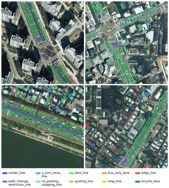
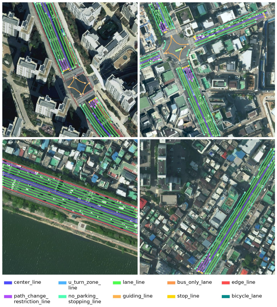
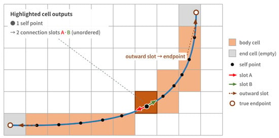
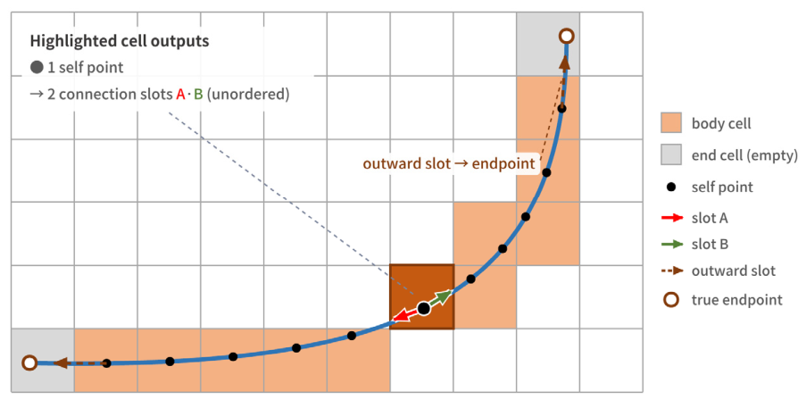
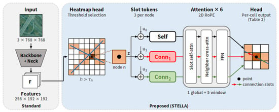
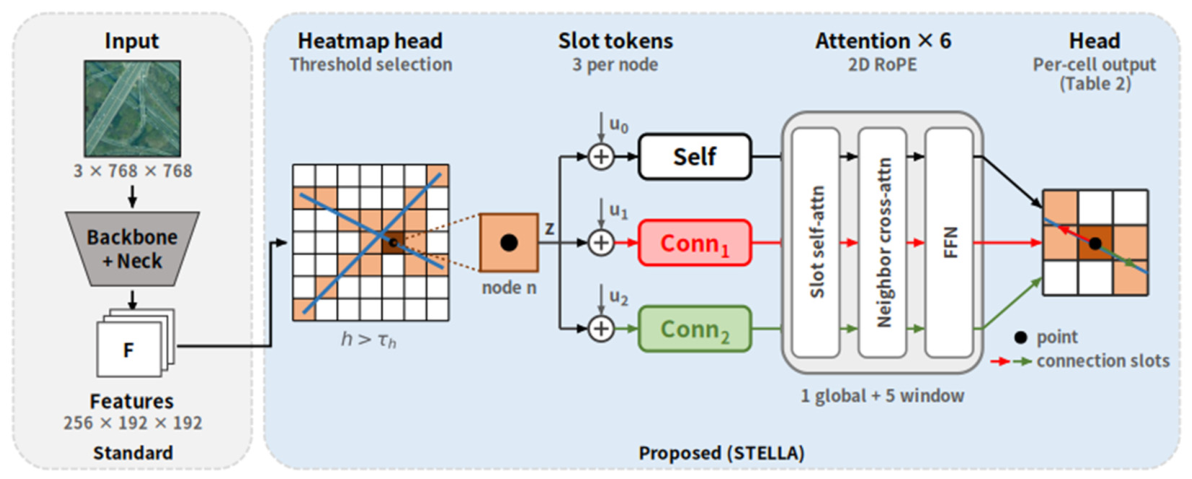
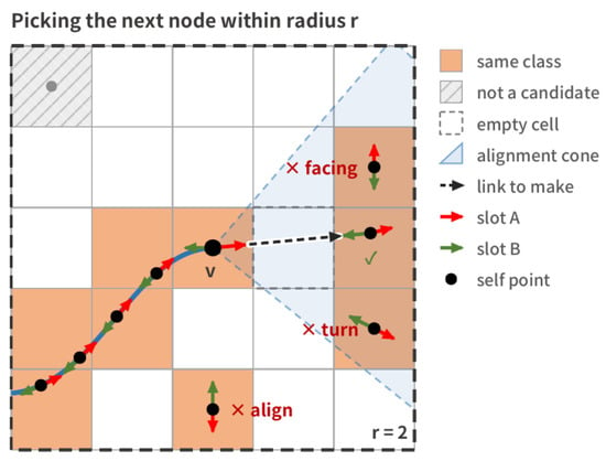
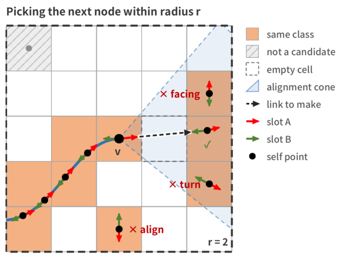
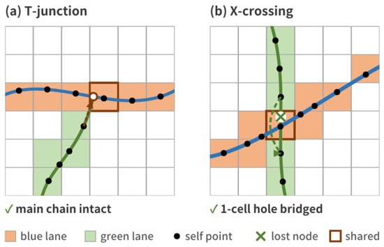
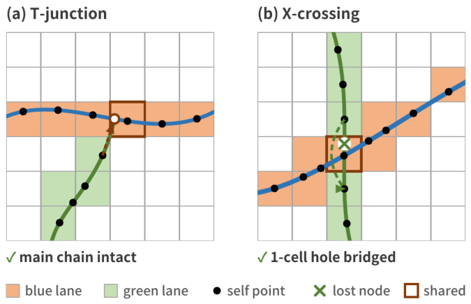
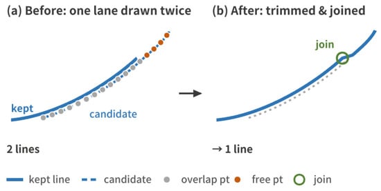
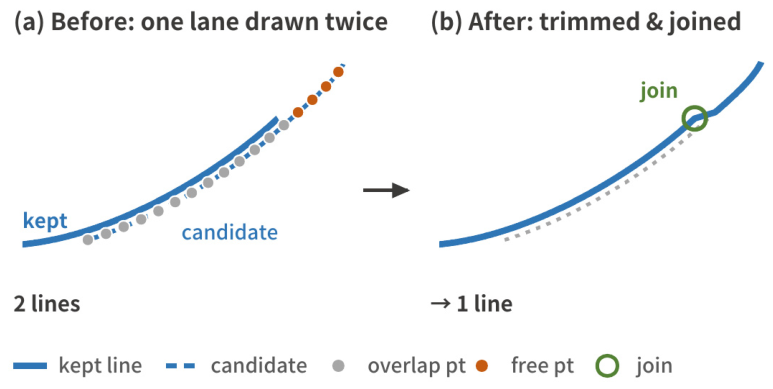
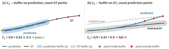
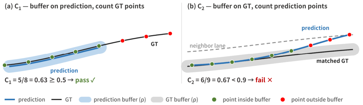
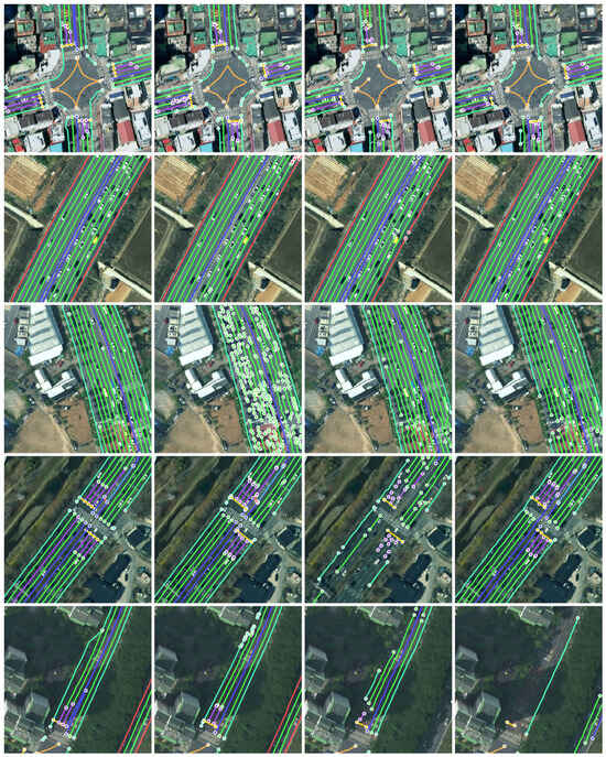
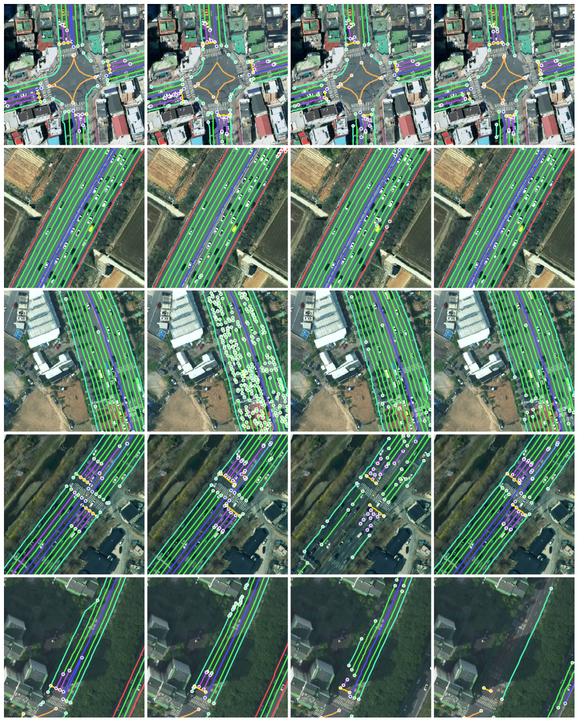
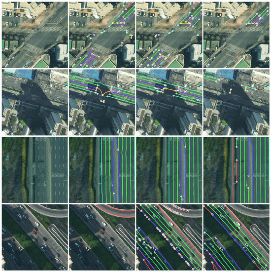
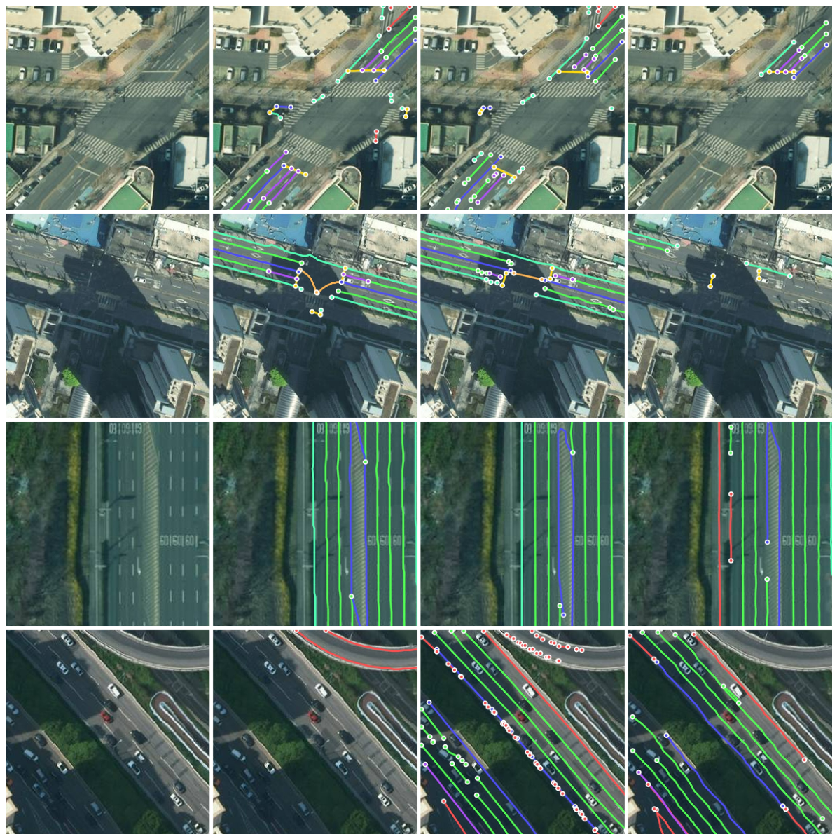

Disclaimer/Publisher’s Note: The statements, opinions and data contained in all publications are solely those of the individual author(s) and contributor(s) and not of MDPI and/or the editor(s). MDPI and/or the editor(s) disclaim responsibility for any injury to people or property resulting from any ideas, methods, instructions or products referred to in the content. |
© 2026 by the authors. Licensee MDPI, Basel, Switzerland. This article is an open access article distributed under the terms and conditions of the Creative Commons Attribution (CC BY) license.