


Highlights
What are the main findings?
- Shaded leaves accounted for 48.2% of total gross primary productivity (GPP) across the Beijing–Tianjin–Hebei region during 2017–2025. Their contribution varied by land cover, from 43.6% in cropland to 53.7% in forest.
- Replacing fixed clumping indices with vegetation-specific seasonal indices reduced the root-mean-square error of GPP estimates in four of five vegetation and crop groups. The largest reductions occurred in forest (5.3%) and shrubland (4.6%).
What are the implications of the main findings?
- The 30 m SS-GPP30 maps reveal differences in sunlit- and shaded-leaf productivity between neighboring vegetation patches that become less distinct at 500 m resolution.
- The 8-day time series distinguishes the seasonal peaks of the two canopy components. Across the region, shaded-leaf GPP peaked in August, about three weeks before sunlit-leaf GPP.
Abstract
Accurate estimation of gross primary productivity (GPP) at fine spatial and temporal resolutions is essential for characterizing carbon uptake across heterogeneous landscapes. Coarse-resolution GPP products smooth differences among neighboring vegetation patches, while many fine-resolution products report only total GPP and do not distinguish the contributions of sunlit and shaded leaves. In this study, we developed SS-GPP30, a spatially continuous dataset that provides 8-day estimates of total GPP and its sunlit- and shaded-leaf components at 30 m resolution across the Beijing–Tianjin–Hebei (BTH) region from 2017 to 2025. The dataset was generated using a two-leaf light-use-efficiency framework driven by Harmonized Landsat and Sentinel-2 (HLS)-derived leaf area index, regional-scale ERA5 meteorological forcing (0.25°), annual 30 m land cover, and seasonal, vegetation-type-specific dynamic representative clumping index. The methodological advance over existing high-resolution GPP products lies in integrating 30 m HLS-based canopy dynamics with sunlit–shaded TL-LUE modeling and seasonal vegetation-type-specific dynamic clumping index, thereby enabling finer temporal representation of canopy photosynthesis and spatial characterization of heterogeneous landscapes. Evaluation against flux-derived GPP at eight eddy covariance sites showed that the seasonal index reduced the root-mean-square error in four of five vegetation and crop groups, with the largest reductions in forest (5.3%) and shrubland (4.6%). Cross-product comparisons across vegetation types yielded values ranging from 0.70 to 0.89, while SS-GPP30 better preserved fine-scale spatial heterogeneity than coarser-resolution products. During 2017–2025, mean annual GPP was 1431.7 g C m−2 yr−1, with sunlit- and shaded-leaf GPP contributing 742.0 and 689.7 g C m−2 yr−1, respectively. Shaded leaves contributed 48.2% of total GPP and showed marked spatiotemporal variation. Both components increased significantly, with a stronger trend in shaded-leaf GPP. Therefore, SS-GPP30 fills an important gap in fine-resolution GPP mapping by providing 30 m estimates of total, sunlit-leaf, and shaded-leaf GPP, thereby resolving both regional vegetation productivity and within-canopy photosynthetic partitioning across the BTH region. The framework also has potential for application to other regions.
1. Introduction
Gross primary productivity (GPP), the rate at which terrestrial vegetation fixes atmospheric carbon through photosynthesis, is the largest component flux of the global land carbon cycle and the energetic foundation of ecosystem growth, food productivity, and many land–atmosphere feedbacks [1,2]. Reliable GPP estimates are therefore needed to quantify carbon budgets, evaluate ecosystem responses to climate variability and disturbance, and support land and crop management. These needs are particularly acute in the Beijing–Tianjin–Hebei (BTH) region, where intensively cultivated plains, rapidly urbanizing corridors, and forested and grass-covered mountains form a heterogeneous landscape. Previous BTH assessments based on the 500 m MODIS GPP record have characterized broad regional patterns and environmental controls [3]. However, the 500 m grid scale cannot resolve many field boundaries, urban–vegetation interfaces, narrow ecological patches, or topographically structured variations that are relevant to regional carbon accounting.
Satellite remote sensing has transformed GPP estimation from sparse site measurements into spatially continuous monitoring. The MODIS productivity-efficiency framework established an operational record by combining absorbed photosynthetically active radiation (APAR) with biome-dependent light-use efficiency and meteorological stress scalars [2,4]. Related models, including the vegetation photosynthesis model and eddy covariance–light-use efficiency model, introduced alternative representations of canopy greenness, water stress, and environmental regulation [5,6,7,8]. These approaches, together with process-based, machine-learning, and solar-induced-fluorescence products, have greatly expanded the capacity to monitor terrestrial photosynthesis. Nevertheless, representative global or continental products generally prioritize coverage and temporal regularity over landscape detail. For example, MOD17A2H provides 8-day GPP at 500 m [3], whereas several other widely used products operate at still coarser resolutions. Mixed pixels can therefore smooth productivity contrasts in fragmented croplands, peri-urban mosaics, and mountainous vegetation.
The light-use-efficiency (LUE) formulation remains attractive for regional mapping because it links satellite-observed canopy state to a concise physiological principle: GPP is the product of APAR and the efficiency with which absorbed radiation is converted to fixed carbon. Its simplicity also exposes an important structural limitation. Conventional “big-leaf” models treat the canopy as a single photosynthetic unit, although irradiance and photosynthetic response differ markedly between sunlit and shaded foliage. The two-leaf LUE (TL-LUE) model addresses this limitation by partitioning leaf area index (LAI) and APAR into sunlit and shaded components with distinct maximum efficiencies [7,9,10]. Evaluations across flux sites and temporal scales show that this representation can reduce sensitivity to illumination conditions and often improves GPP simulation relative to MOD17, although the magnitude of improvement depends on biome and temporal aggregation [11,12,13,14]. Explicit treatment of direct and diffuse radiation further captures their different penetration through the canopy and the nonlinear response of canopy photosynthesis to sky conditions [15,16].
Canopy clumping is central to this partition. The clumping index (CI) describes departures of foliage from a random spatial distribution and controls radiation interception as well as the allocation of leaf area and APAR between sunlit and shaded leaves. Ignoring clumping can substantially bias modeled GPP because the same total leaf area can produce different illuminated and shaded fractions under different canopy architectures [17]. Moreover, CI is not necessarily constant through the year: Phenology changes crown filling, shoot organization, and gap fraction. Recent TL-LUE experiments demonstrate that seasonal CI can reduce errors associated with a constant-CI assumption [18]. Dynamic CI is therefore important for maintaining physical consistency between seasonal canopy structure, radiation partitioning, and component GPP.
Fine spatial resolution and frequent temporal sampling have rarely been combined with this component-level physiology over large, heterogeneous regions. Landsat-based studies have demonstrated 30 m GPP mapping, but cloud contamination and a comparatively sparse revisit cycle complicate continuous sub-seasonal records [19]. Data fusion has produced 30 m, 8-day total GPP for croplands [20], and a recent China-wide dataset provides 30 m total GPP at a monthly step for 2016–2020 [21]. Conversely, a global TL-LUE dataset explicitly separates sunlit and shaded GPP at an 8-day step but uses a 0.05-degree grid [22]. Thus, representative products do not jointly provide 30 m spatial detail, 8-day temporal fidelity, explicit sunlit–shaded separation, and a spatially continuous multiyear regional record. This combination matters: The BTH-wide 30 m maps provide more fine-grained delineation of field boundaries, forest edges, terrain-related gradients, and heterogeneous land-cover mosaics than 500 m products, thereby retaining more spatial heterogeneity and reducing mixed-pixel smoothing.
A key question is how fine-scale patterns of GPP across the BTH region change through the growing season and from year to year. A continuous record at 30 m and 8-day intervals can capture these changes while also providing estimates of sunlit- and shaded-leaf GPP. To address this question, this study aims to (1) integrate Harmonized Landsat and Sentinel-2 (HLS)-derived canopy information, meteorological forcing, land cover, and dynamic CI within TL-LUE; (2) generate spatially continuous 30 m estimates of sunlit-leaf, shaded-leaf, and total GPP for the BTH region at 8-day intervals from 2017 to 2025; and (3) characterize the resulting spatial, seasonal, and interannual variability across major vegetation types. The resulting dataset is hereafter referred to as SS-GPP30 (Sunlit–Shaded GPP at 30 m spatial resolution). The principal contribution is a component-resolved, native 30 m, and temporally consistent GPP dataset and framework that improves the spatial representation of heterogeneous landscapes while retaining 8-day sunlit–shaded process information across nine consecutive years.
2. Materials and Methods
2.1. Study Area
The study domain comprises Beijing Municipality, Tianjin Municipality, and Hebei Province (collectively, the BTH region) in northern China. The region encompasses a variety of landscapes, including densely cultivated plains, urban and peri-urban areas, mountain forests, shrub vegetation, grasslands, and coastal zones. It has a temperate continental monsoon climate, with cold, dry winters and hot, rainy summers. During 1991–2020, the regional mean annual temperature was approximately 13.2 °C and mean annual precipitation was approximately 517.1 mm, with most rainfall concentrated in the warm season [23]. Ecologically, the BTH region connects the croplands of the North China Plain with northern and western mountain forests, grasslands, and the Bohai coastal zone. These ecosystems support food productivity, biodiversity conservation, regional carbon uptake, and ecological protection in one of China’s most densely urbanized regions. These ecological functions are especially important given the region’s water scarcity and intense pressure from land-use change [3,23].
The heterogeneous mosaic of vegetation types, with contrasting canopy structures and seasonal growth patterns, makes BTH a suitable setting for investigating fine-scale spatial variation in GPP and differences in modeled sunlit–shaded GPP partitioning. Rapid economic development and urbanization, accompanied by substantial land-use and land-cover changes, further highlight the need for fine-scale monitoring of vegetation productivity. In addition, multiple flux observation sites within and around the region provide observational support for model parameter calibration and multi-site validation. Figure 1 shows the administrative divisions and corresponding land cover of the BTH region.
Figure 1.
Location and CLCD land-cover (2021) composition of the Beijing–Tianjin–Hebei study area.
2.2. Overall Workflow
Figure 2 summarizes the overall workflow, including multisource data acquisition, HLS preprocessing and LAI retrieval, meteorological and canopy-structure data preprocessing, TL-LUE-based estimation of sunlit, shaded, and total GPP, and comparison with flux observations and reference products.
Figure 2.
Overall workflow of this study.
2.3. Data Sources
Table 1 lists the products, source resolutions, variables, and roles in the analysis. ERA5 rather than ERA5-Land was used because ERA5-Land can contain missing land pixels along the land–sea boundary; the coarser ERA5 grid provided spatially complete forcing over the coastal BTH domain.
Table 1.
Datasets used for TL-LUE modeling, parameter calibration, and product evaluation.
2.3.1. HLS Preprocessing and LAI Retrieval
The HLSS30 and HLSL30 V002 surface-reflectance observations were jointly used, as HLS provides geometrically and radiometrically harmonized observations across sensors at a 30 m spatial resolution [42]. The HLS Fmask [43] quality layer was used to exclude cloud and cloud-shadow pixels. LAI was estimated from the valid HLS reflectance observations using the Canada Centre for Remote Sensing version of the Simplified Level-2 Prototype Processor (SL2P-CCRS) [44]. The processor uses sensor-specific neural networks trained on canopy reflectance simulated by radiative transfer models. SL2P-CCRS uses neural networks trained with simulated canopy reflectance from coupled leaf–canopy radiative transfer models to provide computationally efficient, sensor-specific retrievals of canopy biophysical variables. The valid LAI retrievals were composited into 8-day intervals using the maximum-value compositing method. Gaps in the 8-day LAI time series were first filled by linear interpolation, followed by reconstruction using Whittaker smoothing [45]. At the Yucheng cropland site (CN-Yuc), reconstructed LAI was compared with field measurements on 15 sampling dates in 2024 and 2025 (Pearson’s and RMSE = ; Figure S6).
The SS-GPP30 dataset includes a quality flag (QA) for each 30 m pixel and 8-day period from 2017 to 2025 to indicate how well satellite observations support the reconstructed LAI. A flag of 0 indicates that a valid observation was available during the period and that the absolute difference between the reconstructed LAI and the LAI derived from that observation was within the prescribed threshold. A flag of 1 indicates that this difference exceeded the threshold or that the period fell within a short gap bounded on both sides by valid observations from the same year. A flag of 2 indicates a longer gap, observations on only one side of the gap, or no valid observational support. A value of 255 denotes missing reconstructed LAI. Thresholds varied by land cover and season. We used the area-weighted 90th percentile of absolute fitting residuals as the difference threshold and determined the maximum short-gap length by withholding consecutive observations and repeating the reconstruction. Users can use the flag to screen out GPP estimates with poorly supported LAI inputs.
2.3.2. ERA5 Meteorological Forcing
The meteorological reanalysis dataset used in this study was derived from the fifth-generation European Centre for Medium-Range Weather Forecasts (ECMWF) atmospheric reanalysis (ERA5) dataset, developed by the ECMWF using an advanced Earth system model and a four-dimensional variational data assimilation system [26]. This dataset integrates multiple sources of surface, satellite, and upper-air observations with numerical model simulations to improve the accuracy and spatiotemporal consistency of various meteorological variables at the global scale. In this study, we used hourly 2 m air temperature (, °C), 2 m dew-point temperature (, °C), and both total and diffuse downward shortwave radiation at the surface. In accordance with the method of Zheng et al. [46], vapor pressure deficit (VPD) was calculated from and as follows:
where saturated vapor pressure (SVP) and VPD are in kPa, relative humidity (RH) is expressed as a fraction, and and are in °C. VPD was calculated from hourly and . Hourly and VPD were then averaged over each 8-day period. Air temperature, VPD, and both total and diffuse shortwave radiation were bilinearly resampled to the target 30 m grid. Because resampling adds no new meteorological information at 30 m, the fine-scale spatial detail in SS-GPP30 comes primarily from HLS-derived LAI and annual 30 m land cover. Direct shortwave radiation was calculated as total minus diffuse shortwave radiation. Direct and diffuse photosynthetically active radiation (PAR) were obtained by multiplying the corresponding shortwave radiation components by 0.43, following Bi et al. [22].
Atmospheric CO2 concentrations were obtained from the globally averaged marine surface record of the NOAA Global Monitoring Laboratory (GML) [29].
2.3.3. CLCD and PFT Assignment
The China Land Cover Dataset (CLCD) is the first Landsat-derived annual 30 m land-cover dataset for China. It combines dense Landsat time series, random-forest classification and spatial–temporal filtering to improve temporal consistency. Its reported overall accuracy is 79.31%, and independent comparisons showed that it outperformed several widely used global land-cover products over China [28]. These characteristics provide both the spatial detail and annual consistency needed to represent land-cover heterogeneity and change in the BTH region.
Because CLCD does not distinguish individual crop types, we used the China Crop Dataset–Maize (CCD-Maize) to identify maize pixels in the BTH region. CCD-Maize provides annual maps of maize distribution at 30 m resolution by matching satellite-derived normalized difference vegetation index (NDVI) time series to reference seasonal curves for maize [30]. Combined with the single- and double-cropping classification, these maps determined where and when the GPP model used C4 maize parameters rather than C3 winter wheat parameters. We used the corresponding annual maize maps for 2017–2024. Because a 2025 map was unavailable, we used the 2024 maize distribution for 2025.
Because the CLCD and International Geosphere-Biosphere Programme (IGBP) classification systems use different class definitions, the CLCD categories were associated with their corresponding IGBP classes using the crosswalk in Table 2. The broad CLCD forest category encompasses all IGBP forest types.
Table 2.
Mapping from annual CLCD classes to corresponding IGBP classes.
2.3.4. Clumping Index and Phenology Data
This study used a global 500 m, 8-day CI product derived from MODIS observations. The product retrieves CI with an adjusted kernel-driven bidirectional reflectance distribution function (BRDF) model that improves hotspot representation, while a backup algorithm based on anisotropic flat index and BRDF archetypes constrains abnormal retrievals. Compared with static or annual CI values, its 8-day sequence better represents seasonal changes in canopy structure and is therefore advantageous for temporally explicit partitioning of sunlit and shaded foliage [18,31,32]. Since the latest available year of this CI product is 2023, the subsequent representative CI statistics were based on the 2017–2023 period.
The MCD12Q2 product was additionally used to characterize vegetation phenology. MCD12Q2 provides annual land surface phenology metrics at a spatial resolution of 500 m, derived from time series of the two-band Enhanced Vegetation Index (EVI2) calculated from MODIS nadir BRDF-adjusted reflectance data. The product provides information on key phenological stages, including greenup, maturity, peak greenness, senescence, and dormancy, as well as the number of detected vegetation cycles within each year. Up to two vegetation cycles are recorded for each pixel, enabling the characterization of vegetation with more than one growth cycle [33,34]. In this study, the number of detected vegetation cycles was used to distinguish single-season and double-season systems within cropland identified by CLCD. Cropland pixels with one and two detected vegetation cycles were classified as single-season and double-season systems, respectively, and were subsequently analyzed separately when we extracted representative CI time series.
When mapping regional GPP, we inferred the cropping system of each pixel based on its smoothed 8-day LAI time series for the given year. A double-cropping system requires the presence of two significant growth peaks separated by at least 64 days (8 composites), with a distinct trough between them. Pixels exhibiting at least one qualifying growth peak but lacking a valid pair of peaks were classified as single-season cropland (see Supplementary Text S2 for details).
2.4. TL-LUE Model
To overcome the limitations of treating a canopy as a single homogeneous layer, the TL-LUE model explicitly separates sunlit and shaded foliage. These two canopy components experience different radiation environments and have distinct maximum light-use efficiencies. Total GPP is estimated by summing their contributions [9,22]:
where is absorbed photosynthetically active radiation; the subscripts “su” and “sh” denote sunlit and shaded leaves, respectively; and are their maximum LUE values (g C MJ−1); and are temperature and VPD stress scalars; and is the carbon dioxide fertilization scalar, calculated following the method of Bi et al. [22]. The full equations for calculating sunlit- and shaded-leaf GPP are provided in Text S1.
The PAR absorbed by the two canopy components was calculated as
where and are diffuse and direct PAR, is diffuse PAR below the canopy, is albedo, is the mean leaf–sun angle, is the solar zenith angle, and C represents multiple scattering of direct radiation within the canopy. A spherical leaf-angle distribution was assumed, with .
Total LAI was partitioned into sunlit and shaded components using the dynamic clumping index ():
Environmental constraints on LUE were represented by
The TL-LUE parameters were assigned according to plant functional types. The maximum light-use efficiencies of sunlit and shaded leaves ( and ) and the optimum air temperature () were calibrated using Markov chain Monte Carlo (MCMC) for forests, grasslands, shrublands, and croplands. We used a common parameter set for the mapped forest class because the two-leaf model allows GPP to vary among forest stands through differences in radiation absorption and environmental conditions even when physiological parameters are shared. For a given amount of radiation absorbed by each canopy component and a given set of environmental scalars, GPP is linear in the maximum light-use efficiencies of sunlit and shaded leaves. For croplands, the parameters for winter wheat (C3) and maize (C4) were calibrated separately to account for differences in light-use efficiency between the two photosynthetic pathways. The remaining TL-LUE parameters (, , , , and ) were kept unchanged from the literature-based settings [22,47]. The final TL-LUE parameters used for each vegetation group are summarized in Table 3. Following the approach of Lin et al. [21], we used the annual 30 m CCD-Maize maps to identify maize pixels, which were treated as a proxy for C4 crops. Single-cropped maize pixels were assigned maize parameters throughout the year. Double-cropped maize pixels were treated as winter wheat–summer maize rotations. Based on the seasonal time series at the three cropland flux sites, we applied the maize values of , , and from June to October, and the corresponding winter wheat values during the rest of the year. Other cropland pixels not identified as maize were assigned winter wheat parameters throughout the year as a proxy for C3 crops.
Table 3.
TL-LUE parameters for different vegetation groups. and denote the maximum light-use efficiencies of shaded and sunlit leaves, respectively. is the optimum air temperature, and is canopy albedo (dimensionless). and are the lower and upper air temperature thresholds, respectively. and are the lower and upper vapor pressure deficit thresholds, respectively.
2.5. Extraction of Representative CI Time Series
To reduce the influence of anomalous pixels, spatial autocorrelation, and interannual variability on regional statistics, a combination of high-purity pixel screening, spatial block statistics, and stratified bootstrap resampling [48] was used to extract representative time series of the CI for different vegetation types.
First, high-purity vegetation pixels were selected based on the dominant land-cover type and its fractional coverage derived from the 2017–2023 CLCD dataset. Specifically, the original 30 m CLCD data were aggregated to the 480 m grid. Within each 480 m grid cell, the number of 30 m pixels belonging to each land-cover class was counted, and the corresponding fractional coverage was calculated as the proportion of pixels assigned to that class. The land-cover class with the highest fractional coverage was defined as the dominant land-cover type of the 480 m grid cell. Because the BTH region is predominantly covered by cropland, forest, shrub, and grassland in the CLCD dataset, representative CI time series were extracted for these four land-cover types. For year y and vegetation type k, the set of high-purity pixels was defined as
where denotes the set of high-purity pixels belonging to vegetation type k in year y; i denotes an individual pixel; is the fractional coverage of the dominant land-cover type within pixel i; denotes the dominant land-cover type of pixel i; and k represents one of the four vegetation types: cropland, forest, shrub, or grassland. Only pixels with a dominant land-cover fraction greater than 0.95 were retained for subsequent analysis.
Because cropland includes both single-season and double-season systems, which differ substantially in their phenological cycles and seasonal canopy structural dynamics, cropland pixels were not treated as a single group. Instead, they were further separated into single-season and double-season systems according to phenological information derived from MCD12Q2, and representative CI time series were calculated separately for the two systems. Forest, shrub, and grassland were analyzed directly according to their respective vegetation types.
Quality control was then applied to the CI data for each observation period, retaining only finite values within the physically meaningful range of . To minimize temporal biases caused by changes in the spatial distribution of valid observations, pixels with relatively complete annual observations were further selected within each year. Specifically, only pixels with valid CI observations for at least 80% of the 46 8-day composite periods in a year were retained, thereby maintaining a relatively consistent spatial sample throughout the annual time series.
To account for spatial autocorrelation among neighboring pixels, the study area was divided into non-overlapping pixel blocks. For each year, 8-day period, and vegetation type, the median CI of valid pixels within each spatial block was calculated as
where denotes the median CI of spatial block b, b denotes the block index, and represents the CI value of valid pixel i within the block. For cropland, spatial block statistics were calculated separately for single-season and double-season systems. The use of block-level medians reduces the influence of local outliers and skewed distributions while alleviating spatial pseudoreplication caused by treating a large number of neighboring pixels as independent observations.
The block-level statistics from the same 8-day composite periods during 2017–2023 were then pooled for each vegetation type. A pixel-count-weighted 10% trimmed mean was calculated and used as the representative CI for each composite period. For cropland, this procedure was conducted separately for single-season and double-season systems. Specifically, block-level CI medians were ranked, and the lower and upper 10% of the weighted distribution were removed before we calculated the weighted mean of the remaining blocks. In this analysis, the images were represented in an equal-area projection, so each pixel covered the same area. The number of valid pixels within each spatial block was therefore used as a proxy for its relative spatial contribution. This approach preserves the spatial contribution of different parts of the study area while reducing the influence of extreme block-level values on the representative time series.
The uncertainty of the representative CI was estimated using a two-level stratified bootstrap procedure based on years and spatial blocks. The years from 2017 to 2023 were first resampled with replacement, followed by resampling of spatial blocks within each selected year. The representative CI was recalculated for each resample. This procedure was repeated 500 times, and the 2.5th and 97.5th percentiles of the resulting bootstrap distribution were used to define the 95% confidence interval. These confidence intervals represent the uncertainty associated with the estimated regional representative CI rather than the spatial variability of the original pixel-level CI values.
Finally, 46-point 8-day representative CI time series were obtained for forest, shrub, grassland, single-season cropland, and double-season cropland, and were subsequently used to compare seasonal variations among different vegetation types. The baseline simulation in the sensitivity analysis used these extracted representative CI time series as its CI input. For the site-level comparison, the dynamic configuration used the representative 8-day CI curve assigned to each vegetation or cropping-system class. The static configuration used the corresponding vegetation-type-specific CI value reported by Bi et al. [22] and held this value constant throughout the year.
To assess the effect of applying a common regional CI curve across locations and years, we performed paired TL-LUE simulations for a stratified sample of 30 m pixels from 2017 to 2023. The baseline simulation used the regional seasonal CI curve for the corresponding vegetation type or cropping system. In the second simulation, we matched the center of each sampled pixel to its containing 500 m CI grid cell and used the satellite-derived CI for that cell in the corresponding year and 8-day period. Both simulations used the same LAI, meteorological inputs, and calibrated model parameters. Using only periods valid in both simulations, we compared cumulative GPP and the fraction of cumulative GPP contributed by shaded leaves.
2.6. Reference Products, Flux Comparison, and Accuracy Metrics
We obtained flux-derived GPP from six sites through the FLUXNET Shuttle [35,36,49] and from the Yanshan eddy covariance (EC) dataset provided by the National Ecosystem Science Data Center [37,38]. The Yanshan dataset comprises three sub-sites representing shrubland, evergreen coniferous forest, and mixed tree–shrub forest. We used only the shrubland and evergreen coniferous forest sub-sites and excluded the mixed tree–shrub forest sub-site because its 2021 records exhibited clear data-quality anomalies. Even after we removed all identifiable contamination caused by missing-value codes, mean GPP remained anomalously high during summer late-night hours. Furthermore, no net ecosystem exchange (NEE) observations passed quality control for approximately 224 consecutive days from late May to the end of 2021. Therefore, this sub-site was excluded from the analysis. The eight sites used in this study comprised two forest sites (CN-BeO and the Yanshan planted evergreen coniferous forest site), two grassland sites (CN-Du2 and CN-Xi2), one shrubland site (Yanshan shrub site), and three cropland sites (CN-Lch, CN-Yuc, and CN-Nmn). Site coordinates, IGBP land-cover classes, and observation periods are listed in Table S5. For the six FLUXNET sites, we used GPP derived from daytime flux partitioning [36,50], whereas for the Yanshan sites, we used the GPP provided in the original dataset [37,38].
For the site-level comparisons, we adapted the site-centered sampling approach used in the GPP-net study [51]. For SS-GPP30, we centered a window on the 30 m pixel containing the tower, averaged LAI over the resulting area, and used this mean LAI as input to the TL-LUE model to calculate site-level GPP. The flux footprint is the upwind area that contributes to the flux measured at the tower during a given period. Because the variables needed to estimate a time-varying footprint were unavailable, we used fixed sampling areas for the tower comparisons.
The MOD17A2H GPP product (hereafter MOD-GPP) provided an independent satellite benchmark. It offers spatially continuous, quality-controlled global GPP estimates at 500 m and an 8-day interval, enabling consistent regional and multiyear comparisons. MOD17A2H is also based on a light-use-efficiency formulation and has become one of the most widely used satellite GPP products for ecosystem monitoring and model evaluation [4,39,40].
The Penman–Monteith–Leuning GPP product (hereafter PML-GPP) provided an independent satellite benchmark for ecosystem productivity assessment. It offers spatially continuous, quality-controlled global GPP estimates at 500 m spatial resolution and an 8-day interval, enabling consistent regional and multiyear comparisons. PML-GPP is based on a Penman–Monteith–Leuning framework that couples satellite observations with meteorological forcing and physiological constraints to estimate vegetation carbon uptake. By incorporating both energy and water limitations, PML-GPP has become one of the widely used satellite GPP products for ecosystem carbon cycle studies, productivity monitoring, and model evaluation [41].
The global sunlit and shaded canopy GPP dataset developed by Bi et al. [22] (hereafter Bi2022-GPP) provided an additional satellite-based benchmark for ecosystem productivity assessment. It offers spatially continuous global GPP estimates at 0.05° spatial resolution and an 8-day interval from 1992 to 2020, with monthly and annual aggregates also available, enabling consistent regional and multiyear comparisons. Bi2022-GPP was generated using a revised TL-LUE model driven by GLOBMAP leaf area index, CRUJRA meteorological data, and ESA-CCI land cover. The model separately estimates GPP from sunlit and shaded leaves while accounting for temperature, water stress, and atmospheric CO2 effects on photosynthesis.
Hi-GLASS GPP v1 (hereafter Hi-GLASS GPP) provides a fine-resolution satellite-based benchmark for GPP across China. It offers GPP estimates at 30 m spatial resolution and a monthly interval from 2016 to 2020, allowing fine-scale spatial heterogeneity in ecosystem productivity to be retained more effectively than in conventional coarse-resolution GPP products. The dataset was generated from Landsat observations using the revised eddy covariance–light-use efficiency (rEC-LUE) model [21]. Validation against 90 site-years of observations from 42 eddy covariance flux sites yielded an overall of 0.77 and an RMSE of 50.53 g C m−2 month−1, demonstrating its ability to capture both the magnitude and seasonal variability of GPP across major ecosystem types in China [21].
For n pairs of modeled values and observed or reference values , with respective means and , agreement was quantified using the squared Pearson correlation coefficient (), root-mean-square error (RMSE), and bias:
We evaluated model performance separately for five groups: forest, grassland, shrubland, winter wheat, and maize. For forest, grassland, winter wheat, and maize, we used leave-one-site-out cross-validation. In each fold, we withheld all 8-day observations from one site for validation and calibrated the model parameters using only data from the other sites in that group. For shrubland, which was represented by a single site, we used leave-one-year-out cross-validation. In this approach, we withheld one year at a time and calibrated the parameters using observations from the remaining years. For each group and CI configuration, we pooled the paired predictions and flux-derived GPP observations from all held-out folds and calculated and RMSE from these pairs.
3. Results
3.1. Spatiotemporal Availability of HLS Observations
The multiyear pixel-wise median showed pronounced spatial heterogeneity in clear-sky HLS availability across the BTH region (Figure 3a). Most pixels had 15–59 clear-observation days per year, with higher availability along the western and northern parts of the region and in portions of the northeastern and eastern margins, where the median commonly exceeded 60 days and locally reached 90 days or more. In contrast, broad areas of the central and southern plains were dominated by pixels with 15–44 clear-observation days, with scattered pixels having fewer than 15 days. The stripes associated with overlapping orbital swaths in Figure 3a were not visible in either the reconstructed LAI maps or the final GPP maps.
Figure 3.
Spatial and interannual availability of clear-sky HLS observations across the Beijing–Tianjin–Hebei region during 2017–2025. (a) Pixel-wise median annual number of clear-observation days. (b) Interannual variation in clear-observation days. (c) Area proportions in four observation-availability classes.
The regional median number of clear-observation days increased overall and varied among years (Figure 3b), rising from 26 days in 2017 to more than 40 days after 2021 and reaching 48 days in 2025, with a temporary decline in 2020. The area composition shifted accordingly (Figure 3c). In 2017, most of the region had fewer than 30 clear-observation days, whereas by 2025, the distribution had shifted toward the higher-availability classes, with nearly 60% of the region receiving at least 45 days. The area with at least 30 clear-observation days increased from 36.5% in 2017 to 86.5% in 2025, despite a temporary decrease in 2020. When all valid 8-day LAI windows before reconstruction were pooled across 2017–2025 and weighted by area, 27.9% occurred in spring, 23.2% in summer, 27.9% in autumn, and 21.1% in winter (Figure S5). Although direct observations were not available in every 8-day interval at every pixel, repeated clear-sky observations provided spatially extensive seasonal constraints, particularly after 2021. Together with 8-day compositing, temporal interpolation, and Whittaker smoothing, this coverage was sufficient to support the subsequent regional 8-day LAI and GPP reconstruction.
3.2. Seasonal Dynamics of the Representative Clumping Index
The representative 8-day CI trajectories showed distinct seasonal patterns among vegetation types (Figure 4). Single-season cropland exhibited a broad seasonal decline, with CI decreasing from 0.836 in early January to a minimum of 0.717 in late July before recovering toward winter. The gradual CI decline therefore likely reflects progressive canopy development and increasing foliage aggregation as the crop canopy closes, followed by increasing CI during senescence and harvest. In contrast, double-season cropland exhibited a clear bimodal seasonal pattern, with two distinct minima occurring in mid-May (0.683) and mid-September (0.712), respectively. These two low points were separated by a marked increase in CI during early July. This temporal trajectory agrees with the phenological characteristics of the double-cropping systems widely practiced in the North China Plain [52,53], where two complete crop growth cycles are achieved within a single year. This phenological difference also accounts for the largest divergence between single- and double-season croplands observed in mid-May, when double-season fields had already reached a high level of canopy development during the first growing cycle, whereas single-season fields remained in the early stages of vegetation establishment.
Figure 4.
Representative 8-day seasonal clumping index trajectories of major vegetation types in the BTH region. Lines denote representative CI values, and shaded bands denote 95% confidence intervals from the stratified bootstrap procedure. Cropland is shown separately for single-season and double-season systems.
Forest and shrub exhibited the strongest seasonal variations, reaching their lowest CI values around mid-June (0.502 and 0.478, respectively) and recovering toward winter. Their pronounced summer minima likely reflect leaf expansion and the development of dense, structurally heterogeneous canopies, which increase non-random foliage aggregation, whereas autumn senescence and leaf fall reduce this effect. Grassland showed a much weaker seasonal amplitude, consistent with its relatively low and structurally more homogeneous canopy. Bootstrap intervals were generally narrowest for grassland and widest for shrub, while locally wider intervals for double-season cropland during spring likely reflect spatial variation in crop phenology and management timing.
3.3. Site-Level Validation
The evaluation based on flux-derived GPP showed that incorporating a representative dynamic seasonal CI into the TL-LUE model modestly improved the fit to flux-derived GPP in four of the five vegetation groups (Figure 5). The largest relative reductions in RMSE occurred in forest (5.3%) and shrubland (4.6%), where increased by 0.024 and 0.018 to reach 0.792 and 0.817, respectively. Winter wheat and maize showed similar gains in (0.017 for both), with RMSE decreasing by 2.6% for wheat and 3.0% for maize. Grassland estimates were largely insensitive to the choice of CI configuration. remained close to 0.75 under both configurations, and RMSE differed by only 0.004 g C m−2 d−1.
Figure 5.
Site-level agreement between flux-derived GPP and SS-GPP30 using dynamic and static clumping index configurations in (a) forest, (b) grassland, (c) shrubland, (d) winter wheat and (e) maize. The dashed line denotes 1:1 agreement.
The seasonal comparison showed that the reduction in forest RMSE was consistent across all four seasons and in each year from 2017 to 2021 (Figure S1). The seasonal reduction was largest in spring (0.141 g C m−2 d−1) and smallest in winter (0.036 g C m−2 d−1). For winter wheat, dynamic CI increased spring RMSE by 0.27 g C m−2 d−1 but reduced summer RMSE by 1.91 g C m−2 d−1. For maize, dynamic CI also reduced summer RMSE (by 0.25 g C m−2 d−1), and its annual RMSE was lower in each of the four years evaluated.
The 95% year-block bootstrap intervals for RMSE were 2.14–2.92 g C m−2 d−1 for winter wheat and 3.93–4.94 g C m−2 d−1 for maize (Table S2). These intervals indicate how sensitive the reported errors were to the years sampled at the available sites.
Regarding the specific results for winter wheat and maize, the for winter wheat under the dynamic CI configuration was 0.695, with an RMSE of 2.448 g C m−2 d−1. For maize, the under dynamic CI reached 0.729, and the RMSE under dynamic CI was lower than that of the static CI configuration (4.201 g C m−2 d−1). However, the model still underestimated the highest observed GPP for maize (Figure 5e). This suggests that, although the model captured the overall seasonal variation in maize GPP across sites during leave-one-site-out cross-validation, its ability to reproduce high-productivity periods at individual sites remained limited.
To evaluate SS-GPP30 against another GPP product at the same 30 m spatial resolution, we selected Hi-GLASS GPP, which provides a consistent monthly GPP dataset across China. We compared both products with tower-derived monthly GPP using the same 197 site-month pairs from seven EC sites in and around the BTH region (Figure S2). Correlation with tower-derived GPP was higher for SS-GPP30 in cropland ( versus 0.80) and forest (0.93 versus 0.69). Hi-GLASS GPP captured monthly GPP variation particularly well in grassland and shrubland ( in both), slightly exceeding SS-GPP30 in grassland () and matching it in shrubland (). SS-GPP30 had lower RMSE in all four vegetation types, with values of 92.1 versus 133.3 for cropland, 41.1 versus 93.2 for forest, 13.1 versus 29.1 for grassland, and 13.6 versus 60.8 g C m−2 month−1 for shrubland. These results indicate a regional advantage for the locally calibrated SS-GPP30 in estimating monthly GPP magnitude at the evaluated sites.
3.4. Cross-Product Agreement
Agreement between SS-GPP30 and the three comparison products varied across vegetation types (Figure 6). For PML-GPP, shrubland had the highest correlation () and the lowest RMSE (1.1 g C m−2 d−1), whereas cropland had the lowest correlation () and the highest RMSE (2.3 g C m−2 d−1). For MOD-GPP, ranged from 0.75 over cropland to 0.85 over forest. At high SS-GPP30 values, the fitted lines fell below the line of equality for all four vegetation types, most notably over cropland, where RMSE reached 3.8 g C m−2 d−1. For Hi-GLASS GPP, cropland also had the lowest correlation () and the highest RMSE (3.4 g C m−2 d−1). Across forest, shrubland, and grassland, ranged from 0.79 to 0.86 and RMSE ranged from 1.2 to 1.4 g C m−2 d−1.
Figure 6.
Agreement between SS-GPP30 and three other GPP products across vegetation types from 2017 to 2020. From top to bottom, the rows show PML-GPP, MOD-GPP, and Hi-GLASS GPP. Each point represents the monthly mean of GPP for one pixel, expressed in g C m−2 d−1. Dashed lines indicate the 1:1 reference line, and solid lines indicate the fitted lines.
The agreement between PML-GPP and SS-GPP30 may partly reflect how the two models represent vegetation responses to environmental conditions. PML-GPP is a coupled biophysical model that links GPP and evapotranspiration through canopy conductance [41], while SS-GPP30 uses the TL-LUE framework to constrain photosynthesis through canopy radiation partitioning and environmental stress factors. These representations may lead to similar responses to seasonal variations in canopy development and meteorological conditions. Differences among the products may also reflect their distinct model formulations, input datasets, vegetation parameterizations, and spatial resolutions. For all three comparisons, RMSE was higher over cropland than over forest, shrubland, or grassland, indicating larger differences between product estimates over cropland.
We compared the regional model estimates with Bi2022-GPP to assess how the two products partition total GPP between sunlit and shaded leaves (Figure 7). Across matched 0.05° grid cells and 8-day periods in 2017–2020, Pearson’s r was 0.863 for total GPP, 0.856 for sunlit GPP, and 0.864 for shaded GPP. Shaded leaves accounted for 48.1% of total GPP in our estimates and 54.6% in Bi2022-GPP. The direction of the difference varied by land cover. The shaded share of total GPP was lower in our estimates than in Bi2022-GPP across all latitude bands shown for cropland- and forest-dominated cells. In grassland-dominated cells, our estimate was 2.2 percentage points higher at 38–39°N but lower in each of the three northern bands, with the difference widening from 1.9 percentage points at 40–41°N to 5.3 percentage points at 42–43°N (Figure 7d).
Figure 7.
Comparison of total, sunlit-leaf, and shaded-leaf GPP between SS-GPP30 and Bi2022-GPP across the BTH region, 2017–2020. SS-GPP30 was aggregated to the 0.05° Bi2022-GPP grid using mean resampling. (a–c) Total, sunlit-leaf, and shaded-leaf GPP, respectively. Color indicates the number of paired estimates in each bin, with each pair representing the same grid cell and 8-day period. Dashed lines indicate the 1:1 line. (d) Shaded-leaf GPP as a percentage of total GPP by dominant land-cover type and latitude band.
3.5. Fine-Scale Spatial Detail
The spatial patterns of 30 m SS-GPP30 total, sunlit-leaf, and shaded-leaf GPP are shown for cropland, forest, and grassland windows (Figure 8). In the cropland, total GPP formed a heterogeneous patchwork, with higher values across cultivated areas. Both leaf components retained much of this pattern, while their relative magnitudes varied within the window. In the predominantly forested window, total GPP showed spatially continuous vegetation cover with fine, elongated variations and scattered low-value patches; related variations were visible in both components. The grassland window contained a mosaic of grassland, forest, and cropland in CLCD, accompanied by localized bands and patches of contrasting GPP. The sunlit and shaded maps shared broad spatial features but differed in local contrast.
Figure 8.
Annual mean GPP spatial distributions for cropland, forest, and grassland areas in the BTH region in 2020. (a) Locations of the (b) cropland, (c) forest, and (d) grassland windows.
Compared with SS-GPP30, MOD-GPP showed broader, smoother patches and less distinct boundaries within these windows (Figure 8b–d). Hi-GLASS GPP also retained fine spatial structure, including cropland patch boundaries and elongated variations in the forest and grassland windows, although the distribution and magnitude of GPP differed from those in SS-GPP30. At the same 30 m spatial resolution, SS-GPP30 preserved comparable fine-scale spatial heterogeneity while providing substantially finer temporal information at an 8-day interval rather than the monthly resolution of Hi-GLASS GPP. In addition, SS-GPP30 explicitly separates total GPP into sunlit- and shaded-leaf components, providing additional process-level information on canopy carbon uptake that is not available from Hi-GLASS GPP. These characteristics allow SS-GPP30 to resolve both fine spatial patterns and short-term seasonal dynamics more consistently across heterogeneous landscapes.
To quantify the spatial detail visible in Figure 8b–d, we calculated the fraction of spatial variance in annual mean GPP that was lost when the 30 m maps were averaged to 500 m (Table S4). Aggregation reduced the spatial variance of SS-GPP30 total GPP by 43.88% in the cropland window, 78.50% in the forest window, and 62.23% in the grassland window. For Hi-GLASS GPP, the corresponding reductions over the same valid areas were 38.86%, 70.32%, and 50.53%, respectively. Thus, in all three windows, a larger share of the spatial variation in SS-GPP30 total GPP occurred within individual 500 m cells. This share was largest in the forest window, where a single mean GPP value per 500 m cell concealed nearly four-fifths of the variation mapped at 30 m.
3.6. Spatiotemporal Patterns and Sunlit–Shaded Partitioning of GPP
Mean annual total GPP exhibited a clear regional gradient across the BTH region, with relatively high productivity concentrated over much of the central and southern areas and lower values prevailing in the north and northwest (Figure 9a). This spatial organization was consistently reproduced by both the sunlit- and shaded-leaf components (Figure 9b,c), indicating that the large-scale variation in total GPP was jointly reflected in the two canopy components. Sunlit-leaf GPP was generally greater in magnitude than shaded-leaf GPP, with spatial means of 742.0 and 689.7 g C m−2 yr−1, respectively. Together, these components resulted in a spatial mean total GPP of 1431.7 g C m−2 yr−1 and a median of 1423.0 g C m−2 yr−1.
Figure 9.
Spatial patterns of mean annual GPP in the BTH region during 2017–2025. (a) Total GPP, (b) sunlit-leaf GPP, (c) shaded-leaf GPP, and (d) the contribution of shaded-leaf GPP to total GPP.
Whereas the spatial patterns of absolute GPP were broadly similar, the relative contribution of shaded leaves displayed a distinct spatial structure (Figure 9d). Shaded-leaf contributions were below 50% in 60.2% of mapped pixels, but values above 50% were more common in the northern and northeastern areas, whereas lower contributions occurred more extensively in the northwest and across much of the central and southern region. Overall, shaded leaves contributed an average of 47.3% of total GPP, with an interquartile range of 42.4–53.2%. The mapped values ranged from 25.7% to 58.5%, indicating appreciable spatial variation in the relative roles of sunlit and shaded leaves in canopy carbon uptake. Spatial means and medians of GPP in Figure 9 included valid zero values and excluded NoData pixels, while pixel-level shaded-leaf percentages were calculated only where mean annual total GPP was positive.
Annual mean GPP showed an overall increasing tendency for both sunlit and shaded leaves from 2017 to 2025, despite noticeable interannual fluctuations (Figure 10a). Sunlit-leaf GPP was higher than shaded-leaf GPP in eight of the nine years. Annual means ranged from 1.89 to 2.08 g C m−2 d−1 for sunlit leaves and from 1.77 to 2.07 g C m−2 d−1 for shaded leaves. Both OLS regression and the Mann–Kendall test indicated significant increases in both components, with a larger estimated Sen’s slope for shaded-leaf GPP than for sunlit-leaf GPP (0.0373 versus 0.0234 g C m−2 d−1 yr−1; Table S3). The shaded-leaf contribution to total GPP was 48.1% in 2017 and 50.0% in 2025, but its trend over the nine years was not statistically significant (Sen’s slope percentage points per year and Mann–Kendall ).
Figure 10.
Annual trends and seasonal cycles of sunlit- and shaded-leaf GPP in the BTH region, 2017–2025. (a) Annual regional mean daily GPP for sunlit and shaded leaves (left axis) and the shaded-leaf share of total GPP (right axis). Dotted lines show Sen’s trend estimates, and the reported p values are from Mann–Kendall tests. (b) Mean daily GPP for each 8-day composite period across the nine years. Shaded bands indicate interannual standard deviation.
Both components exhibited pronounced and broadly similar seasonal cycles (Figure 10b). GPP remained low during winter, increased rapidly through spring, and declined after the seasonal peak. Sunlit-leaf GPP was generally higher during spring, whereas shaded-leaf GPP became comparable to or exceeded the sunlit component during the peak growing season. The shaded-leaf component reached its seasonal maximum in August, with the sunlit-leaf peak occurring approximately three weeks later, in early September. Interannual variability was relatively limited during winter but increased substantially during the growing season, particularly around the seasonal peaks.
3.7. Land-Cover Differences in Sunlit–Shaded GPP
Land-cover stratification revealed clear contrasts in both GPP magnitude and the relative contributions of sunlit and shaded leaves (Figure 11). Cropland showed the highest annual mean GPP, followed by forest and grassland, while shrub had the lowest productivity (Figure 11a). Sunlit-leaf GPP was greater than shaded-leaf GPP in cropland and grassland, whereas shaded-leaf GPP was greater in forest and shrub, although the two components were nearly equal in grassland and shrub. Accordingly, the shaded-leaf contribution was highest in forest (53.7%), followed by shrub (50.4%) and grassland (49.1%), and lowest in cropland (43.6%) (Figure 11b). The relatively larger shaded contribution in forest and shrub is consistent with their denser and more vertically structured canopies, which support a greater fraction of photosynthetically active foliage under diffuse or attenuated light. In contrast, the more open and strongly seasonal canopy structure of cropland and grassland tends to favor a larger contribution from sunlit leaves.
Figure 11.
Land-cover differences in sunlit- and shaded-leaf GPP across the Beijing–Tianjin–Hebei region during 2017–2025. (a) Annual mean GPP and its sunlit- and shaded-leaf components for cropland, forest, grassland, and shrub. Whiskers indicate the interannual standard deviation. (b) Shaded-leaf contribution to annual GPP, with gray points representing individual years, diamonds the nine-year mean, and horizontal lines standard deviation. (c–f) Multiyear mean seasonal dynamics of sunlit- and shaded-leaf GPP for cropland, forest, grassland, and shrub, respectively. Shaded ribbons indicate interannual standard deviation.
The seasonal trajectories further emphasized differences among vegetation classes (Figure 11c–f). Cropland exhibited the strongest seasonal amplitude and a pronounced bimodal pattern, which is consistent with the dominant crop phenology of the North China Plain, where winter wheat and summer maize contribute to distinct spring and late-summer productivity peaks. The small but nonzero cropland GPP values observed near the beginning and end of the year likely reflect residual photosynthetic activity of overwintering crops, particularly winter wheat, together with spatial averaging across fields at different phenological stages. Forest showed a broader growing-season plateau, with shaded-leaf GPP becoming comparable to or exceeding the sunlit component during midsummer, when increased canopy development and self-shading enhance the relative importance of shaded foliage. Grassland displayed a smoother seasonal cycle, with both components peaking close together in midsummer, whereas shrub showed a relatively moderate and extended seasonal maximum. Across all classes, interannual variability was limited during winter and increased during the active growing season, with the largest variability occurring in cropland, likely reflecting stronger sensitivity to crop phenology, management, and interannual environmental variability.
4. Discussion
4.1. Seasonal and Vegetation Controls on Sunlit–Shaded GPP Partitioning
The results reveal that the partitioning of canopy photosynthesis between sunlit and shaded foliage varies systematically across seasons, vegetation types, and landscapes in the BTH region. Although sunlit leaves contributed more to annual GPP on average, shaded leaves still accounted for 48.2% of regional total GPP, with substantial spatial variation. Seasonally, sunlit-leaf GPP was generally greater in spring, whereas shaded-leaf GPP became comparable to or exceeded the sunlit component near peak canopy development, indicating a redistribution of photosynthetic activity between contrasting within-canopy light environments over the growing season. Within the TL-LUE framework, this pattern is physically consistent with increasing leaf area and canopy closure, which shift a larger fraction of foliage from direct to attenuated or diffuse radiation and thereby enhance the relative importance of shaded leaves. Previous two-leaf LUE studies have similarly shown that separating sunlit and shaded foliage can improve the representation of canopy photosynthesis because the two leaf groups experience different radiation regimes and photosynthetic efficiencies [54,55]. The present results extend this interpretation to a spatially heterogeneous regional setting and suggest that within-canopy radiation partitioning becomes increasingly important as vegetation approaches its maximum seasonal leaf area.
Differences among vegetation types further support this interpretation. Maximum LUE values calibrated against flux-derived GPP should be interpreted in the context of how the model partitions absorbed radiation within the canopy. If the model underestimates the radiation absorbed by shaded leaves, a higher shaded-leaf maximum LUE can partly compensate when we fit canopy GPP. If we take forest and cropland as an example, differences in their calibrated maximum LUE values may reflect both physiological differences and how the model represents the light environment within each canopy. Forest showed shaded-leaf contributions approaching 54%. In forest, shaded-leaf GPP became comparable to or greater than sunlit-leaf GPP during midsummer, whereas cropland exhibited stronger seasonal fluctuations associated with crop development and the winter wheat–summer maize rotation. These contrasts are consistent with differences in canopy architecture. Woody vegetation generally maintains a deeper and more vertically structured canopy, promoting self-shading and increasing the proportion of foliage operating under diffuse or attenuated light. Cropland and grassland, in contrast, have more open or strongly seasonal canopy structures, particularly outside their peak growth periods, favoring a larger relative contribution from sunlit foliage. Thus, vegetation-specific differences in total GPP reflect not only differences in productivity magnitude and phenology but also differences in how photosynthetic activity is distributed within the canopy.
Both sunlit- and shaded-leaf GPP increased significantly from 2017 to 2025, with a steeper trend for shaded-leaf GPP (Table S3). A pixel was eligible for thinning only if it had at least 12 valid 8-day LAI observations in 2017 and at least 12 in the comparison year. For pixels included in the thinning experiment, reducing each year’s valid LAI window count to its 2017 level changed area-weighted annual mean LAI by % to 0.25%, but reduced annual peak LAI by 1.15–2.66% across the eight comparison years (Figure S4 and Table S1). Annual changes in land cover and atmospheric CO2 may also have contributed to the modeled GPP trends. Because we used a separate CLCD map for each year, changes in the mapped extent of cropland, forest, and other vegetation types could affect regional mean GPP even if mean productivity within each type remained unchanged. For pixels that changed class, the model could also assign a different set of vegetation parameters. In addition, the simulations incorporated year-to-year changes in atmospheric CO2 through a scalar applied to both sunlit- and shaded-leaf GPP. Rising CO2 could therefore have contributed to the increase in both components. To distinguish the contributions of land-cover change and rising CO2, future studies should compare the present results with those from two separate scenarios: one in which land cover is held constant and another in which atmospheric CO2 concentration is held constant.
4.2. Spatial Significance of Fine-Scale Sunlit–Shaded GPP
The spatial variation in sunlit–shaded partitioning provides information that cannot be inferred directly from total GPP alone. The regional patterns of absolute sunlit- and shaded-leaf GPP broadly followed the distribution of total productivity, whereas the shaded-leaf fraction exhibited a distinct spatial pattern, ranging from 25.7% to 58.5%. This divergence indicates that areas with broadly similar levels or spatial patterns of total GPP can differ in the relative contributions of their canopy components. Such differences are difficult to retain in coarse-resolution two-leaf products, where croplands, forest edges, topographic gradients, and small vegetation patches may be combined within a single grid cell. In the forest window, for example, averaging the 30 m estimates to 500 m reduced the spatial variance of annual mean GPP by 81.8% for sunlit leaves and 78.1% for shaded leaves (Table S4). Mapping the two components at 30 m also reveals how the relative contributions of sunlit and shaded leaves can differ between neighboring patches with similar total GPP. Conversely, existing fine-resolution GPP products can preserve landscape heterogeneity but generally provide only total canopy productivity. By resolving both total GPP and its sunlit and shaded components at 30 m, SS-GPP30 therefore connects landscape-scale spatial heterogeneity with the internal partitioning of canopy photosynthesis.
This distinction is particularly relevant in the BTH region, where intensively managed croplands, urban–vegetation interfaces, mountain forests, grasslands, and fragmented vegetation occur within relatively short spatial distances. At coarse resolution, changes in land-cover composition and changes in canopy light environment may both appear simply as changes in grid-cell total GPP. The 30 m component-resolved estimates allow these sources of heterogeneity to be examined more explicitly by retaining individual landscape features while simultaneously describing the relative contribution of sunlit and shaded foliage. The value of the fine spatial resolution is therefore not merely improved delineation of field or vegetation boundaries; rather, it enables canopy-level photosynthetic partitioning to be interpreted in the context of landscape structure.
Taken together, these results show that resolving sunlit and shaded foliage provides a complementary dimension for interpreting regional GPP variability. Total GPP describes the magnitude of canopy carbon uptake, whereas its partitioning provides information on how that uptake is distributed between different canopy light environments. The spatial, seasonal, and vegetation-specific contrasts identified here demonstrate that this partitioning contains information that would be obscured if the canopy were represented only as a single photosynthetic unit. At the same time, because the estimated partitioning depends explicitly on canopy structural parameters, its interpretation requires consideration of uncertainty in the clumping index and associated radiation partitioning. The sensitivity of the estimated GPP components to CI variability is therefore examined in the following section.
4.3. Role and Sensitivity of the Dynamic Clumping Index
A seasonal CI curve allows the TL-LUE model to account for changes in canopy clumping during the growing season when estimating the radiation absorbed by sunlit and shaded leaves. Compared with the vegetation-type-specific static CI configuration, dynamic CI yielded lower RMSE in four of the five vegetation or crop groups, with the largest relative reductions in forest and shrubland and little change in grassland (Figure 5). Although the gains in total GPP accuracy were modest, forest RMSE was lower in all four seasons and in each year from 2017 to 2021 (Figure S1). This consistency suggests that representing seasonal changes in clumping may be particularly useful for structurally complex canopies such as forests, although the evidence is limited to the sites evaluated here.
Perturbing the regional representative CI curves within their bootstrap distributions produced modest changes in mean total GPP (Figure 12a). Across the tested percentiles, the response remained within approximately 3% of the baseline for single-season cropland, double-season cropland, forest, and grassland. Shrubland showed the largest response, ranging from to . Sunlit-leaf GPP was more responsive than total GPP in all five groups. These results describe the effect of uncertainty in the estimated regional curves; they do not indicate how closely a regional curve represents an individual pixel-year.
Figure 12.
Sensitivity of total, shaded-leaf, and sunlit-leaf GPP to variation in the representative dynamic CI across vegetation types. Columns show the relative changes in (a) total GPP, (b) shaded-leaf GPP, and (c) sunlit-leaf GPP compared with the baseline simulation, while rows represent single-season cropland, double-season cropland, forest, grassland, and shrub. Curves show the response across the tested CI percentile range, with open symbols marking selected percentiles. The vertical dashed line indicates P50, and the horizontal line denotes no change from BASE.
Across 11,031 sampled pixel-years, the paired comparison with local, year-specific CI revealed differences that were not apparent from the regional perturbation experiment (Figure S3). In forest, replacing the regional curve increased cumulative GPP by a median of 2.5%, but the 10th–90th percentile range extended from to . The forest shaded-leaf share changed by a median of percentage points, with a range of to percentage points between the 10th and 90th percentiles. In grassland, the median change in shaded-leaf share was instead positive ( percentage points). Thus, even when regional mean GPP is only weakly sensitive to uncertainty in the regional CI curves, replacing a regional curve with local, year-specific CI can substantially change cumulative GPP and the shaded-leaf share at individual locations.
4.4. Limitations and Future Directions
Although SS-GPP30 provides spatially continuous, component-resolved GPP estimates at 30 m resolution, several limitations should be acknowledged.
First, although the evaluation included eight EC sites, each vegetation type was represented by only one to three independent sites. Repeated 8-day observations characterize variation within a site but do not increase the number of independent sites available for testing differences between CI configurations. It therefore remains uncertain whether the modest improvements observed here would persist at other sites of the same vegetation type.
Second, in the production simulations, all pixels within a given vegetation type or cropping-system class share the same seasonal CI curve, which is repeated each year. Figure S3 shows that this simplification can affect local estimates of cumulative GPP and the fraction contributed by shaded leaves. Nevertheless, site-level validation indicates that the model captures much of the observed variation in total GPP, with values ranging from 0.695 to 0.817 across the five vegetation and crop groups.
Third, the ERA5 meteorological forcing has a native spatial resolution of 0.25°, and its resampling to the 30 m grid does not introduce additional fine-scale meteorological information. Consequently, the 30 m spatial heterogeneity represented by SS-GPP30 is primarily constrained by the HLS-derived LAI and annual 30 m land-cover information, while ERA5 provides spatially complete and temporally consistent regional-scale meteorological forcing. This configuration supports consistent regional modeling but may smooth local-scale meteorological variability.
Fourth, at 30 m resolution, small urban green spaces may fall within mixed pixels classified as impervious surfaces, potentially leading to underestimation of local GPP. Higher-resolution land-cover data could help identify these green spaces and estimate their contributions to GPP. Because no wetland flux sites were available for parameter calibration in the study area and wetlands identified by CLCD accounted for less than 0.1% of the BTH region, we used the grassland parameter set to estimate wetland GPP. This approximation introduces uncertainty into local estimates. Improved wetland identification and parameter calibration would benefit from higher-resolution, more accurate wetland maps and wetland flux observations.
Fifth, we retrieved LAI using SL2P-CCRS, which accounts for crown heterogeneity and foliage clumping in forests [56]. In dense canopies, the optical signal can approach saturation at high LAI, adding uncertainty to estimates of peak LAI and peak GPP. Although field validation was limited to the Yucheng cropland site (CN-Yuc), the reconstructed LAI tracked the variation in field measurements across 15 sampling dates in 2024 and 2025 (Pearson’s and RMSE ; Figure S6).
Future work should incorporate additional biome-specific flux sites, direct observational constraints on sunlit–shaded GPP partitioning, contemporaneous spatially explicit CI observations, and, where available, higher-resolution meteorological forcing to further characterize and reduce model uncertainty. The framework has potential for application beyond BTH. However, its transferability remains unverified and requires independent evaluation across additional regions and vegetation types in future studies.
5. Conclusions
This study developed SS-GPP30, a spatially continuous gross primary productivity dataset that resolves total, sunlit-leaf, and shaded-leaf GPP at 30 m spatial resolution and 8-day intervals across the Beijing–Tianjin–Hebei region from 2017 to 2025. By integrating HLS-derived LAI, ERA5 meteorological forcing, annual 30 m land cover, and a dynamic clumping index within the TL-LUE framework, SS-GPP30 combines fine-scale landscape representation with explicit within-canopy photosynthetic partitioning. This framework was designed to retain both the spatial heterogeneity of the BTH landscape and the seasonal dynamics of sunlit and shaded canopy components.
Across the eight flux sites, the benefit of using a seasonal rather than a fixed clumping index varied by vegetation type. Root-mean-square error in total GPP declined in four of the five groups, most notably in forest (5.3%) and shrubland (4.6%), whereas grassland estimates changed little. Across vegetation types, comparisons with PML-GPP, MOD-GPP, and Hi-GLASS GPP yielded values ranging from 0.70 to 0.89, while the 30 m estimates preserved more fine-scale spatial heterogeneity than coarse-resolution products. These comparisons support the capability of SS-GPP30 to represent regional GPP variability while retaining field boundaries, vegetation edges, and other heterogeneous landscape features.
The resulting dataset revealed substantial spatial, seasonal, and vegetation-specific variation in sunlit–shaded GPP partitioning. Mean annual total GPP across the region was , of which sunlit and shaded leaves contributed and , respectively. Shaded leaves accounted for an average of 48.2% of total GPP, but their contribution varied spatially from 25.7% to 58.5%. Both sunlit- and shaded-leaf GPP increased significantly during 2017–2025. The increase was steeper for shaded-leaf GPP, although its share of total GPP showed no significant trend. Clear differences were also observed among vegetation types: Shaded-leaf contributions were higher in forest and shrub and lower in cropland and grassland, while their seasonal trajectories reflected distinct canopy and phenological dynamics.
The sensitivity analysis further showed that uncertainty in the representative clumping index had a relatively limited effect on total GPP for most vegetation types. Overall, SS-GPP30 provides a fine-resolution and component-resolved representation of terrestrial productivity that complements conventional total-GPP products by explicitly describing how canopy carbon uptake is distributed between sunlit and shaded foliage.
Supplementary Materials
The following supporting information can be downloaded at https://www.mdpi.com/article/10.3390/rs18223979/s1. Text S1: Two-Leaf Light Use Efficiency model. Text S2: Identification of single and double cropping from LAI. Figure S1: Seasonal (left) and interannual (right) differences in SS-GPP30 fitting error, expressed as static minus dynamic RMSE and absolute bias. Panels (g) and (h) distinguish winter wheat (solid lines) and maize (dashed lines). Figure S2: Comparison of monthly GPP estimates from SS-GPP30 and Hi-GLASS-GPP against eddy covariance tower estimates across four vegetation types. Panels show (a) cropland, (b) forest, (c) grassland, and (d) shrubland. Blue circles denote SS-GPP30 and open orange triangles denote Hi-GLASS-GPP. Both products were evaluated using the same site-month pairs within each vegetation type. Figure S3: Sensitivity of cumulative GPP and its shaded-leaf share to local, year-specific clumping indices. Changes are shown for (a) cumulative gross primary productivity (GPP) and (b) the fraction of cumulative GPP contributed by shaded leaves when a regional, vegetation-type-specific clumping index (CI) curve is replaced with satellite-derived CI for the corresponding location and year. Positive values indicate higher estimates with local CI. Points denote weighted medians and horizontal bars span the 10th–90th percentiles across sampled pixel-years (11,031 in total), with area weighting within years and equal weighting across years. Both simulations use the same valid 8-day periods. Figure S4: Changes in reconstructed annual mean and peak LAI after thinning 2018–2025 observations to match 2017 observation counts at each pixel. Figure S5: Seasonal availability and distribution of valid 8-day LAI observations in the Beijing–Tianjin–Hebei region, 2017–2025. Figure S6: Comparison of reconstructed HLS/SL2P-CCRS LAI with field measurements at the Yucheng cropland site (CN-Yuc) in 2024 and 2025. Table S1: Effect of thinning observations to 2017 levels on reconstructed LAI. Thinning was restricted to pixels with at least twelve valid 8-day LAI observations in both 2017 and the comparison year. The number of pixels included varied by year because only those with more observations than in 2017 were thinned to their own 2017 count. Table S2: Year-block bootstrap summaries of held-out SS-GPP30 performance under dynamic CI by vegetation group. Values are medians across bootstrap replicates, with 95% bootstrap confidence intervals in brackets. Table S3: Trends in regional mean GPP and the shaded-leaf GPP share in the BTH region during 2017–2025. Slopes were estimated from nine annual values using ordinary least squares (OLS) regression and Sen’s method. Values in brackets indicate 95% confidence intervals. Mann–Kendall p-values were calculated using an exact two-sided test. Both slopes and their 95% confidence intervals are expressed in g C m−2 d−1 yr−1 for GPP and in percentage points per year for the shaded-leaf share of total GPP. Table S4: Spatial variance of 2020 annual mean daily GPP before and after aggregation from 30 to 500 m in the three landscape windows in Figure 8. Variance lost (%) is the share of 30 m spatial variance occurring within 500 m cells: . Both variances are expressed in and weighted by valid area. Only 500 m cells fully inside the window with at least 50% common valid coverage were included. Table S5: Basic information on the flux sites used in this study.
Author Contributions
Conceptualization, F.Y. and Z.J.; methodology, F.Y., Z.J. and C.W.; software, F.Y.; validation, F.Y., X.D. and G.Z.; formal analysis, F.Y.; investigation, F.Y. and M.D.; data curation, F.Y. and J.J.; writing—original draft preparation, F.Y.; writing—review and editing, F.Y., Z.J., C.W., X.D., G.Z., M.D. and J.J.; visualization, F.Y.; supervision, Z.J.; project administration, Z.J.; and funding acquisition, Z.J. All authors have read and agreed to the published version of the manuscript.
Funding
This work was supported by the General Program of the National Natural Science Foundation of China (Grant No. 42471352), the Major Program of the National Natural Science Foundation of China (Grant No. 42090013), and the Open Fund of State Key Laboratory of Remote Sensing Science and Digital Earth, Beijing Engineering Research Center for Global Land Remote Sensing Products (Grant No. OF202501).
Data Availability Statement
The SS-GPP30 dataset generated in this study is publicly available from Science Data Bank (DOI: https://doi.org/10.57760/sciencedb.0193o, accessed on 18 November 2026).
Acknowledgments
We thank NASA’s Land Processes Distributed Active Archive Center (LP DAAC) for providing the HLS, MCD12Q2, and MOD17A2H products; the Copernicus Climate Change Service (C3S) for the ERA5 reanalysis; the developers of the CLCD, PML-V2, and Hi-GLASS GPP datasets for making their data publicly available; and Google for providing the Google Earth Engine platform used for data access and preprocessing. We also thank the site teams who shared their flux observations through the FLUXNET Shuttle. The Yanshan flux dataset was provided by the National Ecosystem Science Data Center, National Science & Technology Infrastructure of China (https://www.nesdc.org.cn). This study contains modified Copernicus Sentinel data (2017–2025) and modified Copernicus Climate Change Service information (2026). Neither the European Commission nor ECMWF is responsible for any use that may be made of the Copernicus information or data it contains.
Conflicts of Interest
The authors declare no conflicts of interest.
References
- Beer, C.; Reichstein, M.; Tomelleri, E.; Ciais, P.; Jung, M.; Carvalhais, N.; Rödenbeck, C.; Arain, M.A.; Baldocchi, D.; Bonan, G.B.; et al. Terrestrial Gross Carbon Dioxide Uptake: Global Distribution and Covariation with Climate. Science 2010, 329, 834–838. [Google Scholar] [CrossRef] [Scilit] [PubMed]
- Zhu, W.; Xie, Z.; Zhao, C.; Zheng, Z.; Qiao, K.; Peng, D.; Fu, Y.H. Remote Sensing of Terrestrial Gross Primary Productivity: A Review of Advances in Theoretical Foundation, Key Parameters and Methods. GISci. Remote Sens. 2024, 61, 2318846. [Google Scholar] [CrossRef] [Scilit]
- Guo, H.; Cao, C.; Xu, M.; Yang, X.; Chen, Y.; Wang, K.; Duerler, R.S.; Li, J.; Gao, X. Spatiotemporal Distribution Pattern and Driving Factors Analysis of GPP in Beijing–Tianjin–Hebei Region by Long-Term MODIS Data. Remote Sens. 2023, 15, 622. [Google Scholar] [CrossRef] [Scilit]
- Running, S.W.; Nemani, R.R.; Heinsch, F.A.; Zhao, M.; Reeves, M.; Hashimoto, H. A Continuous Satellite-Derived Measure of Global Terrestrial Primary Production. BioScience 2004, 54, 547–560. [Google Scholar] [CrossRef] [Scilit]
- Xiao, X.; Hollinger, D.; Aber, J.; Goltz, M.; Davidson, E.A.; Zhang, Q.; Moore, B., III. Satellite-Based Modeling of Gross Primary Production in an Evergreen Needleleaf Forest. Remote Sens. Environ. 2004, 89, 519–534. [Google Scholar] [CrossRef] [Scilit]
- Yuan, W.; Liu, S.; Zhou, G.; Zhou, G.; Tieszen, L.L.; Baldocchi, D.; Bernhofer, C.; Gholz, H.; Goldstein, A.H.; Goulden, M.L.; et al. Deriving a Light Use Efficiency Model from Eddy Covariance Flux Data for Predicting Daily Gross Primary Production across Biomes. Agric. For. Meteorol. 2007, 143, 189–207. [Google Scholar] [CrossRef] [Scilit]
- Pei, Y.; Dong, J.; Zhang, Y.; Yuan, W.; Doughty, R.; Yang, J.; Zhou, D.; Zhang, L.; Xiao, X. Evolution of Light Use Efficiency Models: Improvement, Uncertainties, and Implications. Agric. For. Meteorol. 2022, 317, 108905. [Google Scholar] [CrossRef] [Scilit]
- Tian, Z.; Yi, C.; Fu, Y.; Kutter, E.; Krakauer, N.Y.; Fang, W.; Zhang, Q.; Luo, H. Fusion of Multiple Models for Improving Gross Primary Production Estimation with Eddy Covariance Data Based on Machine Learning. J. Geophys. Res. Biogeosci. 2023, 128, e2022JG007122. [Google Scholar] [CrossRef] [Scilit]
- He, M.; Ju, W.; Zhou, Y.; Chen, J.M.; He, H.; Wang, S.; Wang, H.; Guan, D.; Yan, J.; Li, Y.; et al. Development of a Two-Leaf Light Use Efficiency Model for Improving the Calculation of Terrestrial Gross Primary Productivity. Agric. For. Meteorol. 2013, 173, 28–39. [Google Scholar] [CrossRef] [Scilit]
- Huang, L.; Lin, X.; Jiang, S.; Liu, M.; Jiang, Y.; Li, Z.L.; Tang, R. A Two-Stage Light-Use Efficiency Model for Improving Gross Primary Production Estimation in Agroecosystems. Environ. Res. Lett. 2022, 17, 104021. [Google Scholar] [CrossRef] [Scilit]
- Zhou, Y.; Wu, X.; Ju, W.; Chen, J.M.; Wang, S.; Wang, H.; Yuan, W.; Black, T.A.; Jassal, R.; Ibrom, A.; et al. Global Parameterization and Validation of a Two-Leaf Light Use Efficiency Model for Predicting Gross Primary Production across FLUXNET Sites. J. Geophys. Res. Biogeosci. 2016, 121, 1045–1072. [Google Scholar] [CrossRef] [Scilit]
- Guan, X.; Chen, J.M.; Shen, H.; Xie, X. A Modified Two-Leaf Light Use Efficiency Model for Improving the Simulation of GPP Using a Radiation Scalar. Agric. For. Meteorol. 2021, 307, 108546. [Google Scholar] [CrossRef] [Scilit]
- Bao, S.; Ibrom, A.; Wohlfahrt, G.; Koirala, S.; Migliavacca, M.; Zhang, Q.; Carvalhais, N. Narrow but Robust Advantages in Two-Big-Leaf Light Use Efficiency Models over Big-Leaf Light Use Efficiency Models at Ecosystem Level. Agric. For. Meteorol. 2022, 326, 109185. [Google Scholar] [CrossRef] [Scilit]
- Huang, L.; Yuan, W.; Zheng, Y.; Zhou, Y.; He, M.; Jin, J.; Huang, X.; Chen, S.; Liu, M.; Guan, X.; et al. A Dynamic-Leaf Light Use Efficiency Model for Improving Gross Primary Production Estimation. Environ. Res. Lett. 2024, 19, 014066. [Google Scholar] [CrossRef] [Scilit]
- Liu, Q.; Zhang, Z.; Fan, M.; Wang, Q. The Divergent Estimates of Diffuse Radiation Effects on Gross Primary Production of Forest Ecosystems Using Light-Use Efficiency Models. Geophys. Res. Lett. 2021, 48, e2021GL093864. [Google Scholar] [CrossRef] [Scilit]
- Xu, H.; Zhang, Z.; Wu, X.; Wan, J. Light Use Efficiency Models Incorporating Diffuse Radiation Impacts for Simulating Terrestrial Ecosystem Gross Primary Productivity: A Global Comparison. Agric. For. Meteorol. 2023, 332, 109376. [Google Scholar] [CrossRef] [Scilit]
- Chen, J.M.; Mo, G.; Pisek, J.; Liu, J.; Deng, F.; Ishizawa, M.; Chan, D. Effects of Foliage Clumping on the Estimation of Global Terrestrial Gross Primary Productivity. Glob. Biogeochem. Cycles 2012, 26, GB1019. [Google Scholar] [CrossRef] [Scilit]
- Li, Z.; Jiao, Z.; Wang, C.; Yin, S.; Guo, J.; Tong, Y.; Gao, G.; Tan, Z.; Chen, S. Seasonal Effect of the Vegetation Clumping Index on Gross Primary Productivity Estimated by a Two-Leaf Light Use Efficiency Model. Remote Sens. 2023, 15, 5537. [Google Scholar] [CrossRef] [Scilit]
- Shirkey, G.; John, R.; Chen, J.; Dahlin, K.; Abraha, M.; Sciusco, P.; Lei, C.; Reed, D.E. Fine Resolution Remote Sensing Spectra Improves Estimates of Gross Primary Production of Croplands. Agric. For. Meteorol. 2022, 326, 109175. [Google Scholar] [CrossRef] [Scilit]
- He, M.; Kimball, J.S.; Maneta, M.P.; Maxwell, B.D.; Moreno, A.; Beguería, S.; Wu, X. Regional Crop Gross Primary Productivity and Yield Estimation Using Fused Landsat–MODIS Data. Remote Sens. 2018, 10, 372. [Google Scholar] [CrossRef] [Scilit]
- Lin, S.; Huang, X.; Wang, C.; He, T.; Zhang, X.; Shen, R.; Peng, Q.; Chen, X.; Zheng, Y.; Dong, J.; et al. A 30-m gross primary production dataset from 2016 to 2020 in China. Sci. Data 2024, 11, 1065. [Google Scholar] [CrossRef] [Scilit] [PubMed]
- Bi, W.; He, W.; Zhou, Y.; Ju, W.; Liu, Y.; Liu, Y.; Zhang, X.; Wei, X.; Cheng, N. A global 0.05° dataset for gross primary production of sunlit and shaded vegetation canopies from 1992 to 2020. Sci. Data 2022, 9, 213. [Google Scholar] [CrossRef] [Scilit] [PubMed]
- Wu, H.; Long, B.; Huang, N.; Lu, N.; Qian, C.; Pan, Z.; Men, J.; Zhang, Z. Impacts of Climate Change on Ecological Water Use in the Beijing–Tianjin–Hebei Region in China. Water 2024, 16, 319. [Google Scholar] [CrossRef] [Scilit]
- Masek, J.G.; Ju, J.; Roger, J.C.; Skakun, S.; Vermote, E.; Claverie, M.; Dungan, J.; Yin, Z.; Freitag, B.; Justice, C. HLS-2 Landsat Operational Land Imager Surface Reflectance and TOA Brightness Daily Global 30 m v2.0; Data Set; NASA Land Processes Distributed Active Archive Center: Sioux Falls, SD, USA, 2021. [Google Scholar] [CrossRef] [Scilit]
- Masek, J.G.; Ju, J.; Roger, J.C.; Skakun, S.; Vermote, E.; Claverie, M.; Dungan, J.; Yin, Z.; Freitag, B.; Justice, C. HLS Sentinel-2 Multi-Spectral Instrument Surface Reflectance Daily Global 30 m v2.0; Data Set; NASA Land Processes Distributed Active Archive Center: Sioux Falls, SD, USA, 2021. [Google Scholar] [CrossRef] [Scilit]
- Hersbach, H.; Bell, B.; Berrisford, P.; Hirahara, S.; Horányi, A.; Muñoz-Sabater, J.; Nicolas, J.; Peubey, C.; Radu, R.; Schepers, D.; et al. The ERA5 Global Reanalysis. Q. J. R. Meteorol. Soc. 2020, 146, 1999–2049. [Google Scholar] [CrossRef] [Scilit]
- Hersbach, H.; Bell, B.; Berrisford, P.; Biavati, G.; Horányi, A.; Muñoz Sabater, J.; Nicolas, J.; Peubey, C.; Radu, R.; Rozum, I.; et al. ERA5 Hourly Data on Single Levels from 1940 to Present; Data Set; Copernicus Climate Change Service (C3S) Climate Data Store: Reading, UK, 2023. [Google Scholar] [CrossRef]
- Yang, J.; Huang, X. The 30 m Annual Land Cover Dataset and Its Dynamics in China from 1990 to 2019. Earth Syst. Sci. Data 2021, 13, 3907–3925. [Google Scholar] [CrossRef] [Scilit]
- Lan, X.; Tans, P.; Thoning, K.W. Trends in Globally-Averaged CO2 Determined from NOAA Global Monitoring Laboratory Measurements; NOAA Global Monitoring Laboratory: Boulder, CO, USA, 2026. [Google Scholar] [CrossRef]
- Peng, Q.; Shen, R.; Li, X.; Ye, T.; Dong, J.; Fu, Y.; Yuan, W. A twenty-year dataset of high-resolution maize distribution in China. Sci. Data 2023, 10, 658. [Google Scholar] [CrossRef] [Scilit] [PubMed]
- Jiao, Z.; Dong, Y.; Schaaf, C.B.; Chen, J.M.; Román, M.; Wang, Z.; Zhang, H.; Ding, A.; Erb, A.; Hill, M.J.; et al. An Algorithm for the Retrieval of the Clumping Index (CI) from the MODIS BRDF Product Using an Adjusted Version of the Kernel-Driven BRDF Model. Remote Sens. Environ. 2018, 209, 594–611. [Google Scholar] [CrossRef] [Scilit]
- Gao, G.; Jiao, Z.; Li, Z.; Wang, C.; Guo, J.; Zhang, X.; Ding, A.; Tan, Z.; Chen, S.; Yang, F.; et al. A Phenologically Simplified Two-Stage Clumping Index Product Derived from the 8-Day Global MODIS-CI Product Suite. Remote Sens. 2025, 17, 233. [Google Scholar] [CrossRef] [Scilit]
- Moon, M.; Zhang, X.; Henebry, G.M.; Liu, L.; Gray, J.M.; Melaas, E.K.; Friedl, M.A. Long-term continuity in land surface phenology measurements: A comparative assessment of the MODIS land cover dynamics and VIIRS land surface phenology products. Remote Sens. Environ. 2019, 226, 74–92. [Google Scholar] [CrossRef] [Scilit]
- Friedl, M.; Gray, J.; Sulla-Menashe, D. MODIS/Terra+Aqua Land Cover Dynamics Yearly L3 Global 500m SIN Grid V061; NASA Land Processes Distributed Active Archive Center: Sioux Falls, SD, USA, 2022. [Google Scholar] [CrossRef]
- FLUXNET. FLUXNET Data Shuttle: Download Data; FLUXNET Data Portal: Berkeley, CA, USA, 2026. [Google Scholar]
- Pastorello, G.; Trotta, C.; Canfora, E.; Chu, H.; Christianson, D.; Cheah, Y.-W.; Poindexter, C.; Chen, J.; Elbashandy, A.; Humphrey, M.; et al. The FLUXNET2015 dataset and the ONEFlux processing pipeline for eddy covariance data. Sci. Data 2020, 7, 225. [Google Scholar] [CrossRef] [Scilit] [PubMed]
- Du, J.; Luo, W.; An, Z.; Zhang, L.; Huang, H.; Hao, Y.; Wang, Y. A Dataset of Carbon and Water Fluxes over Typical Ecosystems in Beijing Yanshan Hilly Regions (2020–2021); Dataset; Original Title in Chinese; National Ecosystem Science Data Center: Beijing, China, 2024. [Google Scholar] [CrossRef]
- Du, J.; Luo, W.; An, Z.; Zhang, L.; Huang, H.; Hao, Y.; Wang, Y. A dataset of carbon and water fluxes over typical ecosystems in Beijing Yanshan hilly regions (2020–2021). China Sci. Data 2023, 8, 1–9, (In Chinese with English Abstract). [Google Scholar] [CrossRef] [Scilit]
- Running, S.W.; Mu, Q.; Zhao, M. MOD17A2H MODIS/Terra Gross Primary Productivity 8-Day L4 Global 500 m SIN Grid V006; Data Set; NASA Land Processes Distributed Active Archive Center: Sioux Falls, SD, USA, 2015. [Google Scholar] [CrossRef] [Scilit]
- Running, S.W.; Mu, Q.; Zhao, M. MODIS/Terra Gross Primary Productivity 8-Day L4 Global 500 m SIN Grid V061; Data Set; NASA Land Processes Distributed Active Archive Center: Sioux Falls, SD, USA, 2021. [Google Scholar] [CrossRef]
- Zhang, Y.; Kong, D.; Gan, R.; Chiew, F.H.S.; McVicar, T.R.; Zhang, Q.; Yang, Y. Coupled Estimation of 500 m and 8-Day Resolution Global Evapotranspiration and Gross Primary Production in 2002–2017. Remote Sens. Environ. 2019, 222, 165–182. [Google Scholar] [CrossRef] [Scilit]
- Claverie, M.; Ju, J.; Masek, J.G.; Dungan, J.L.; Vermote, E.F.; Roger, J.C.; Skakun, S.V.; Justice, C. The Harmonized Landsat and Sentinel-2 Surface Reflectance Data Set. Remote Sens. Environ. 2018, 219, 145–161. [Google Scholar] [CrossRef] [Scilit]
- Qiu, S.; Zhu, Z.; He, B. Fmask 4.0: Improved Cloud and Cloud Shadow Detection in Landsats 4–8 and Sentinel-2 Imagery. Remote Sens. Environ. 2019, 231, 111205. [Google Scholar] [CrossRef] [Scilit]
- Djamai, N.; Fernandes, R.; Sun, L.; Hong, G.; Brown, L.A.; Morris, H.; Dash, J. On the consistency and stability of vegetation biophysical variables retrievals from Landsat-8/9 and Sentinel-2. ISPRS J. Photogramm. Remote Sens. 2025, 224, 329–347. [Google Scholar] [CrossRef] [Scilit]
- Eilers, P.H.C. A Perfect Smoother. Anal. Chem. 2003, 75, 3631–3636. [Google Scholar] [CrossRef] [Scilit] [PubMed]
- Zheng, Y.; Shen, R.; Wang, Y.; Li, X.; Liu, S.; Liang, S.; Chen, J.M.; Ju, W.; Zhang, L.; Yuan, W. Improved Estimate of Global Gross Primary Production for Reproducing Its Long-Term Variation, 1982–2017. Earth Syst. Sci. Data 2020, 12, 2725–2746. [Google Scholar] [CrossRef] [Scilit]
- Wu, X.; Ju, W.; Zhou, Y.; He, M.; Law, B.E.; Black, T.A.; Margolis, H.A.; Cescatti, A.; Gu, L.; Montagnani, L.; et al. Performance of linear and nonlinear two-leaf light use efficiency models at different temporal scales. Remote Sens. 2015, 7, 2238–2278. [Google Scholar] [CrossRef] [Scilit]
- McRoberts, R.E.; Magnussen, S.; Tomppo, E.O.; Chirici, G. Parametric, Bootstrap, and Jackknife Variance Estimators for the k-Nearest Neighbors Technique with Illustrations Using Forest Inventory and Satellite Image Data. Remote Sens. Environ. 2011, 115, 3165–3174. [Google Scholar] [CrossRef] [Scilit]
- Yu, G.R.; Wen, X.F.; Sun, X.M.; Tanner, B.D.; Lee, X.; Chen, J.Y. Overview of ChinaFLUX and evaluation of its eddy covariance measurement. Agric. For. Meteorol. 2006, 137, 125–137. [Google Scholar] [CrossRef] [Scilit]
- Lasslop, G.; Reichstein, M.; Papale, D.; Richardson, A.D.; Arneth, A.; Barr, A.; Stoy, P.C.; Wohlfahrt, G. Separation of net ecosystem exchange into assimilation and respiration using a light response curve approach: Critical issues and global evaluation. Glob. Change Biol. 2010, 16, 187–208. [Google Scholar] [CrossRef] [Scilit]
- Wang, S.; Ryu, Y.; Dechant, B.; Zhang, H.; Feng, H.; Lee, J.; Choi, C. GPP-net: A robust high-resolution GPP estimation network for Sentinel-2 using only surface reflectance and photosynthetically active radiation. Remote Sens. Environ. 2026, 334, 115198. [Google Scholar] [CrossRef] [Scilit]
- Sun, H.; Zhang, X.; Chen, S.; Pei, D.; Liu, C. Effects of harvest and sowing time on the performance of the rotation of winter wheat–summer maize in the North China Plain. Ind. Crop. Prod. 2007, 25, 239–247. [Google Scholar] [CrossRef] [Scilit]
- Fan, Y.; Yang, Z.; Lo, M.H.; Hur, J.; Im, E.S. Applying double cropping and interactive irrigation in the North China Plain using WRF4.5. Geosci. Model Dev. 2024, 17, 6929–6947. [Google Scholar] [CrossRef] [Scilit]
- Ma, Y.; Guan, X.; Chen, J.M.; Ju, W.; Huang, W.; Shen, H. Improving MODIS Gross Primary Productivity by Bridging Big-Leaf and Two-Leaf Light Use Efficiency Models. J. Geophys. Res. Biogeosci. 2024, 129, e2023JG007737. [Google Scholar] [CrossRef] [Scilit]
- Zhang, S.; Wang, W.; Yuan, J.; Bai, Y. Global Optimization of a Water-Constrained Two-Leaf Light Use Efficiency Model through Multi-Biome FLUXNET Observations. Agric. For. Meteorol. 2025, 375, 110845. [Google Scholar] [CrossRef] [Scilit]
- Fernandes, R.; Djamai, N.; Harvey, K.; Hong, G.; MacDougall, C.; Shah, H.; Sun, L. Evidence of a bias-variance trade off when correcting for bias in Sentinel 2 forest LAI retrievals using radiative transfer models. Remote Sens. Environ. 2024, 305, 114060. [Google Scholar] [CrossRef] [Scilit]
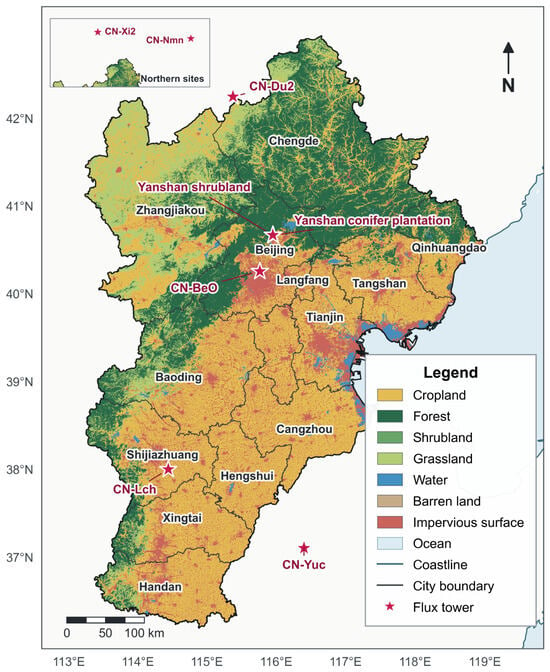
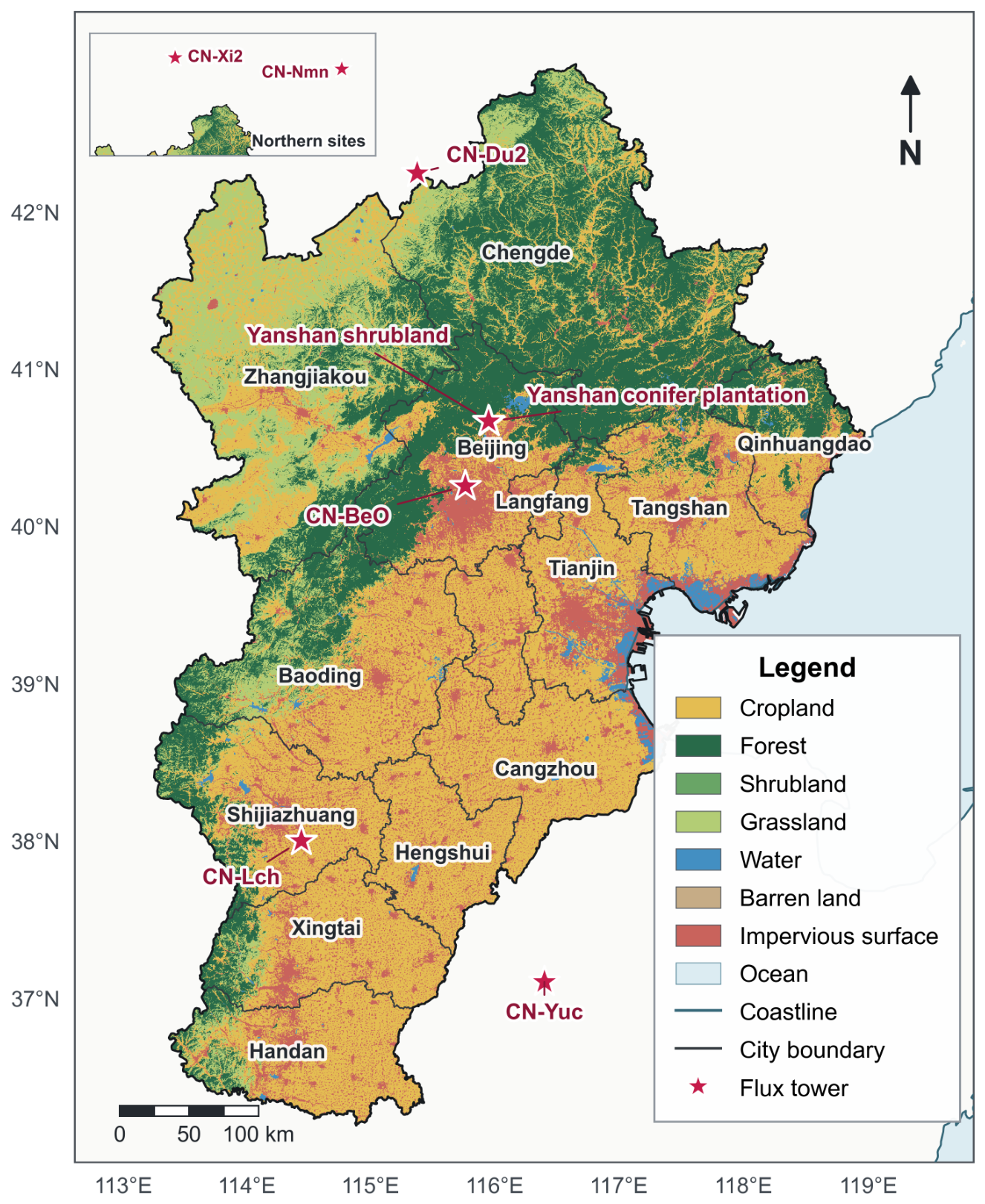
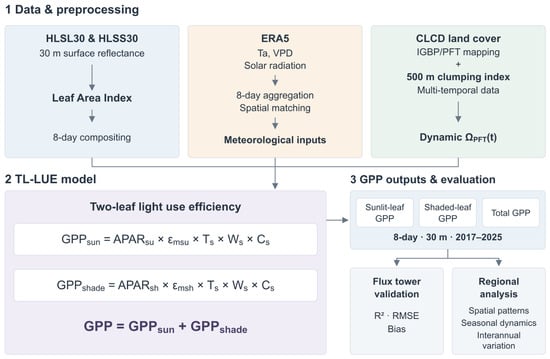
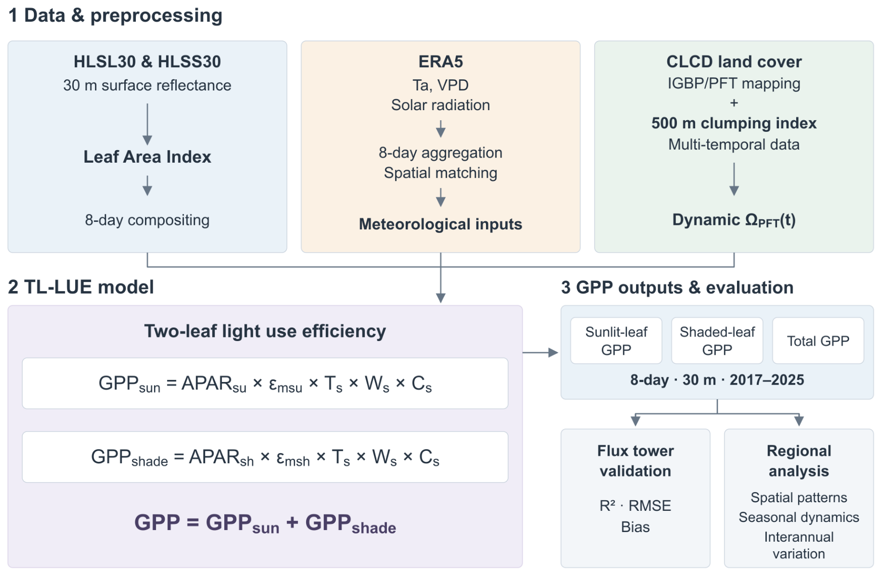
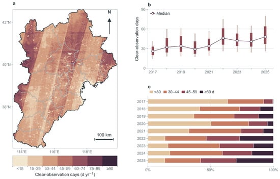
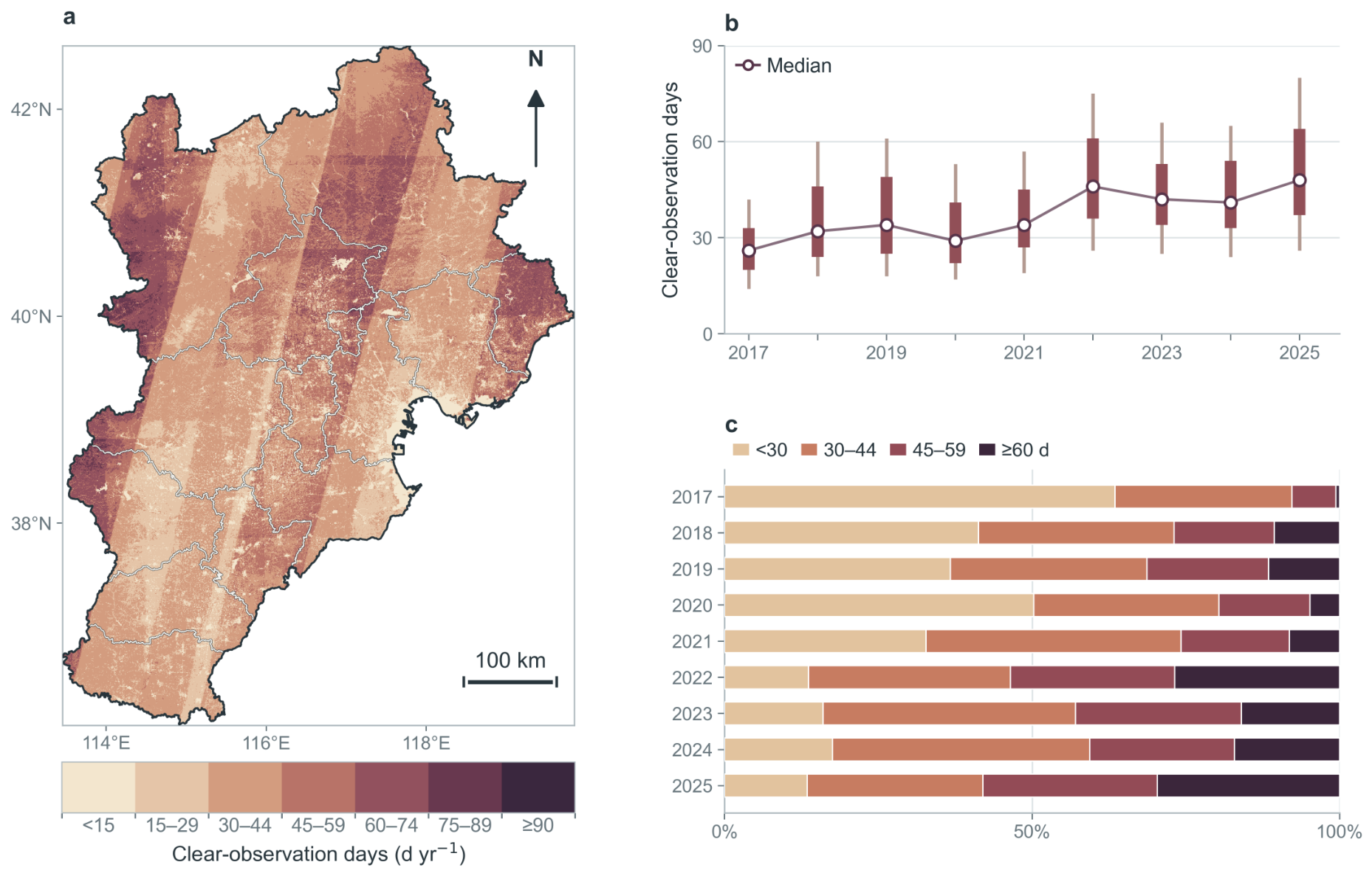
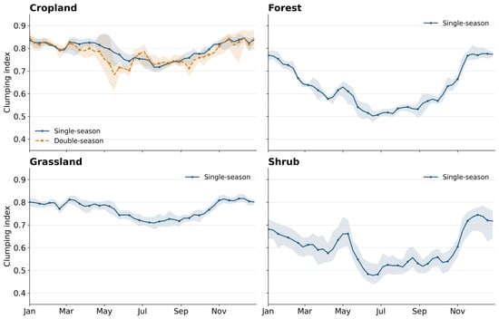
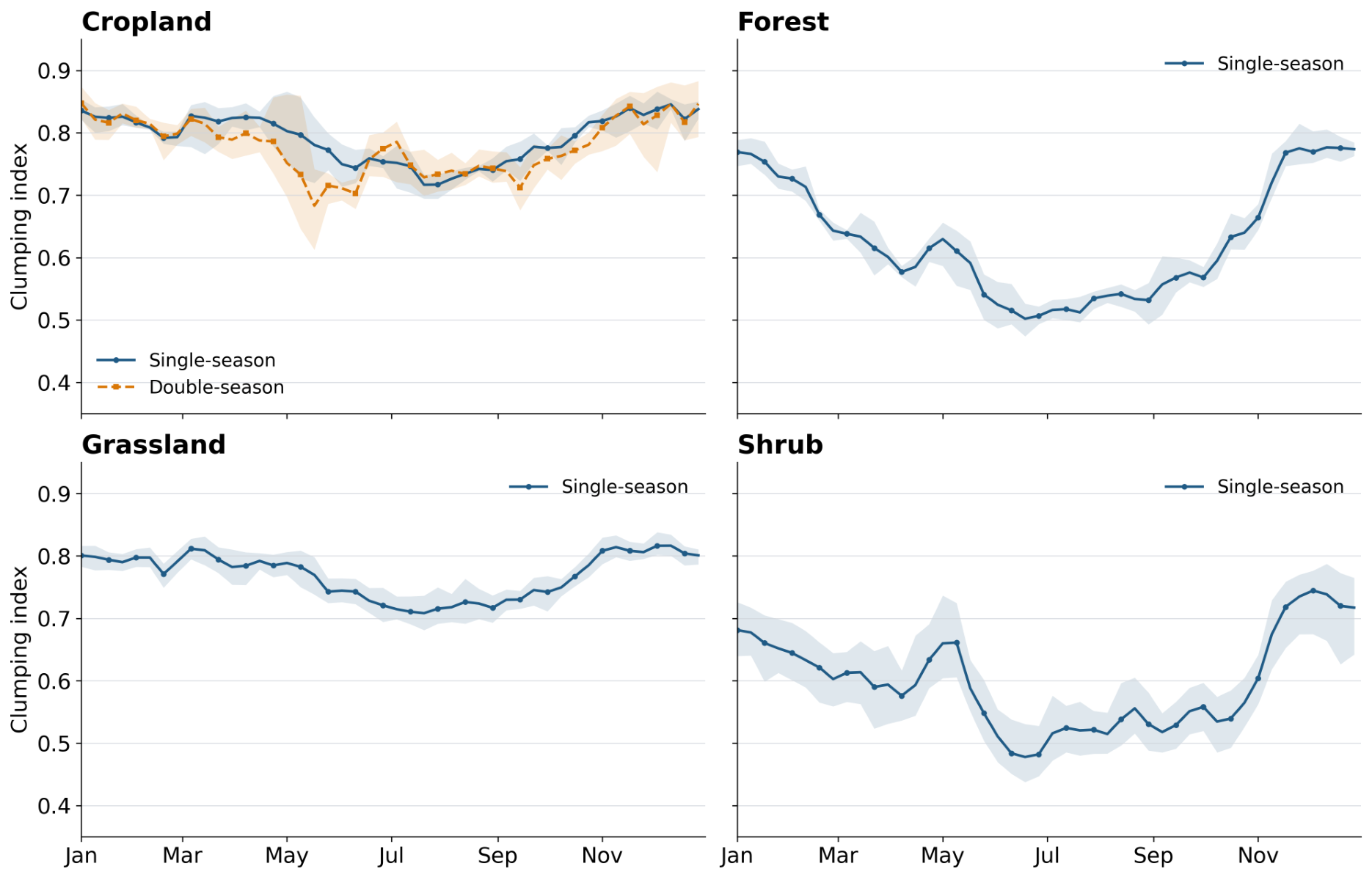
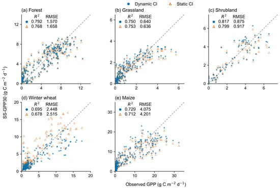
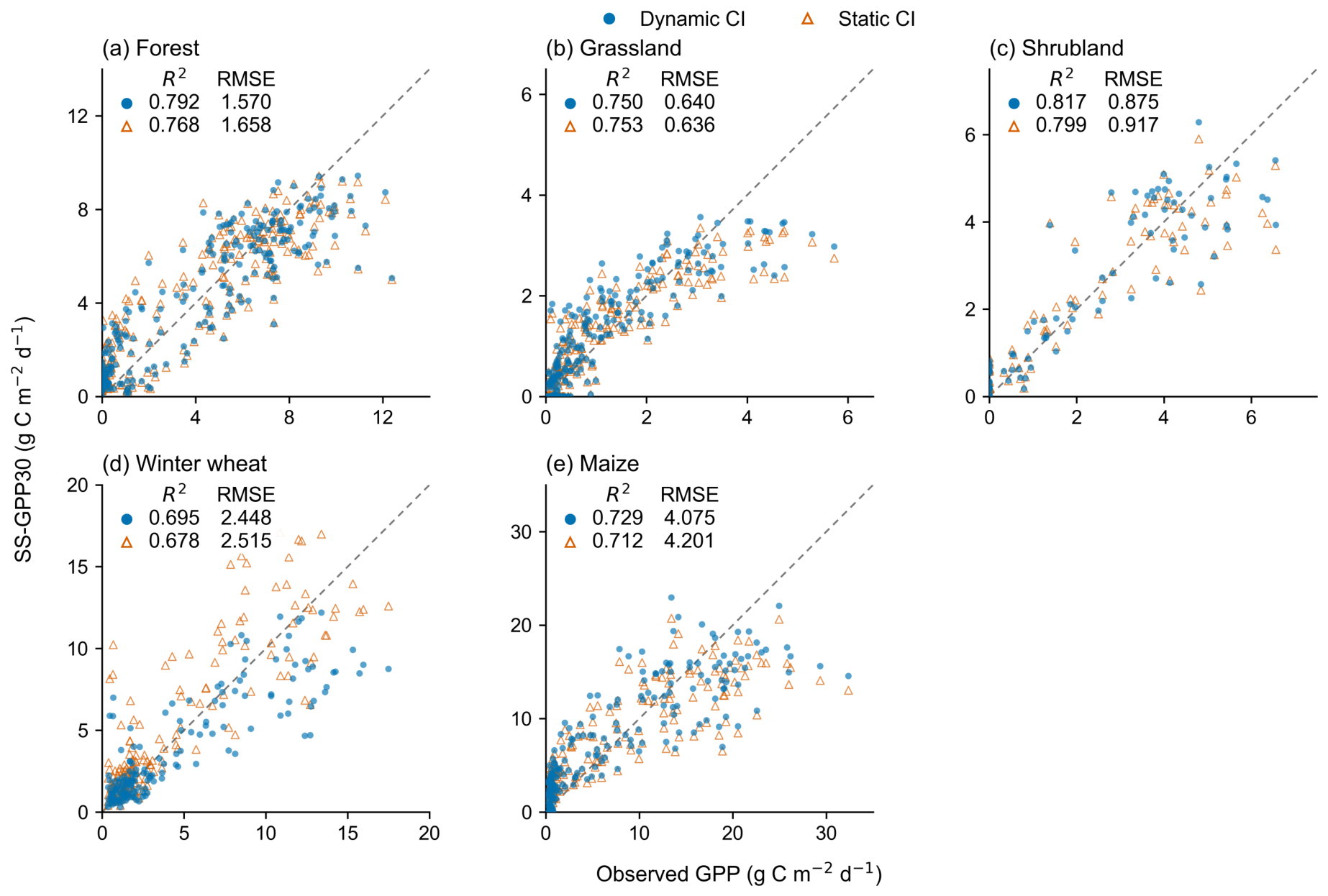
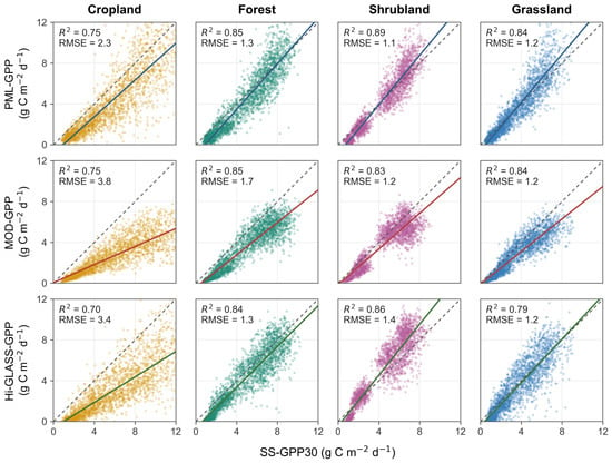
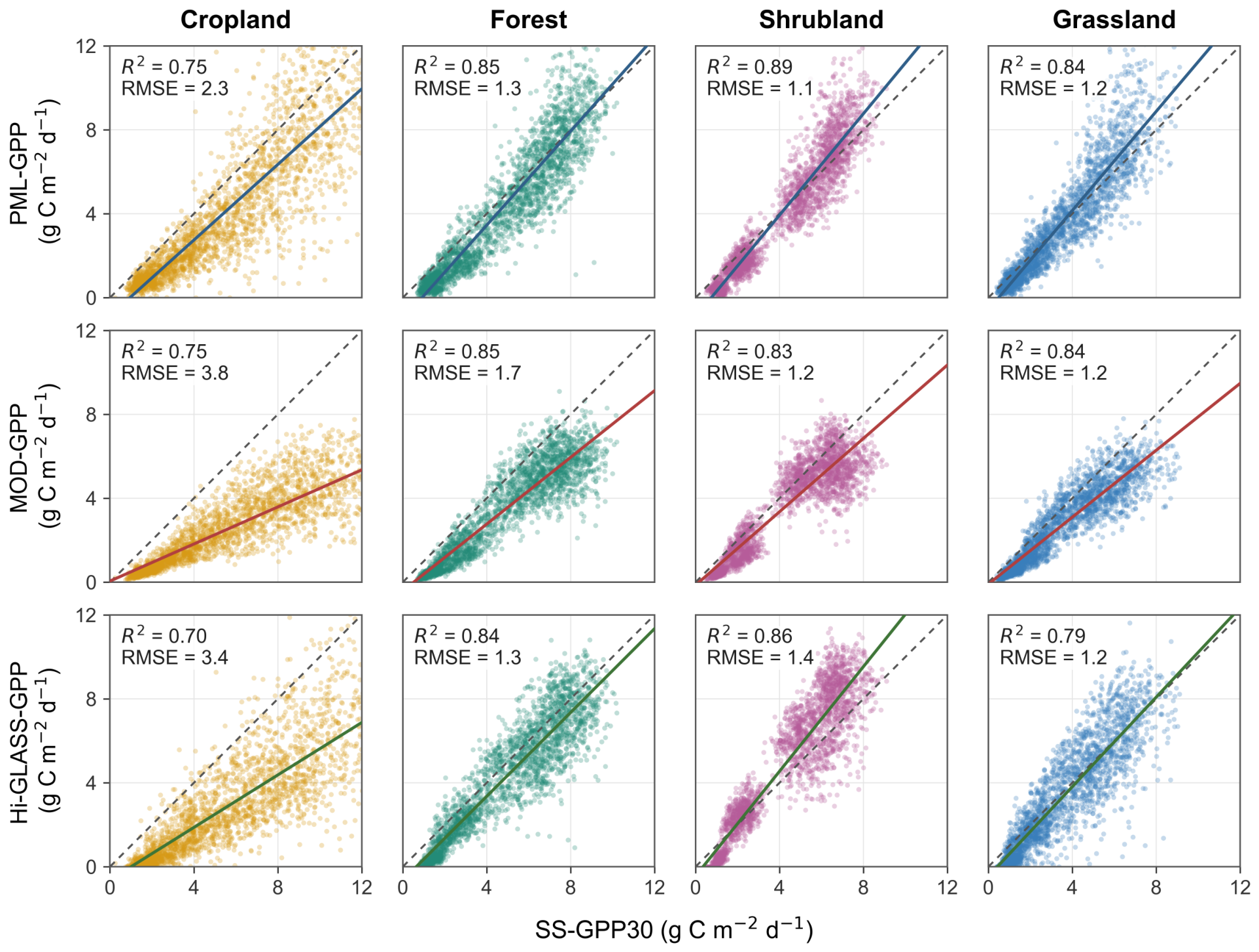
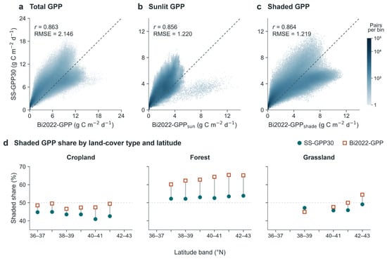
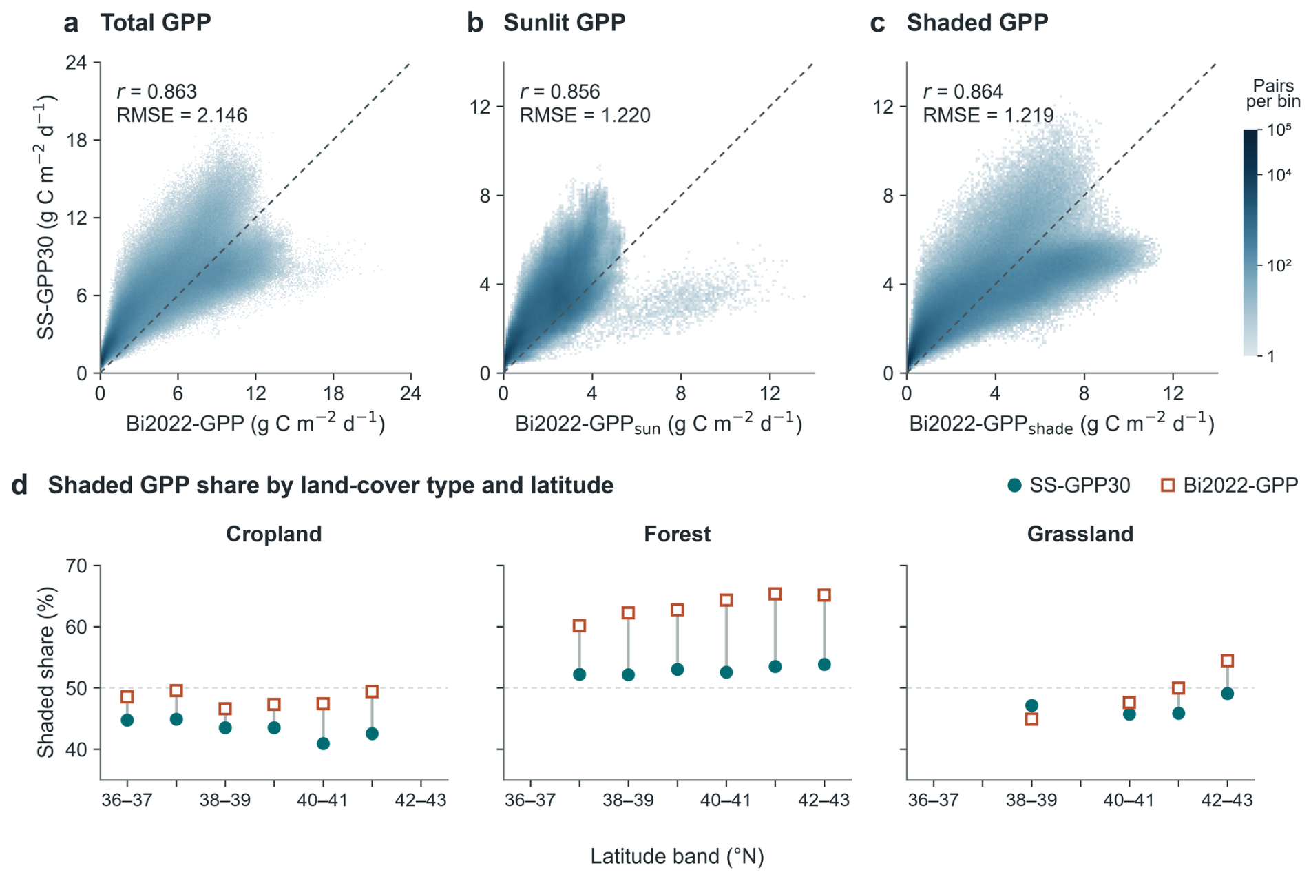
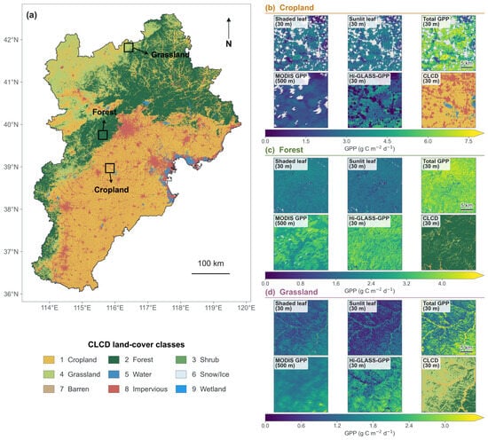
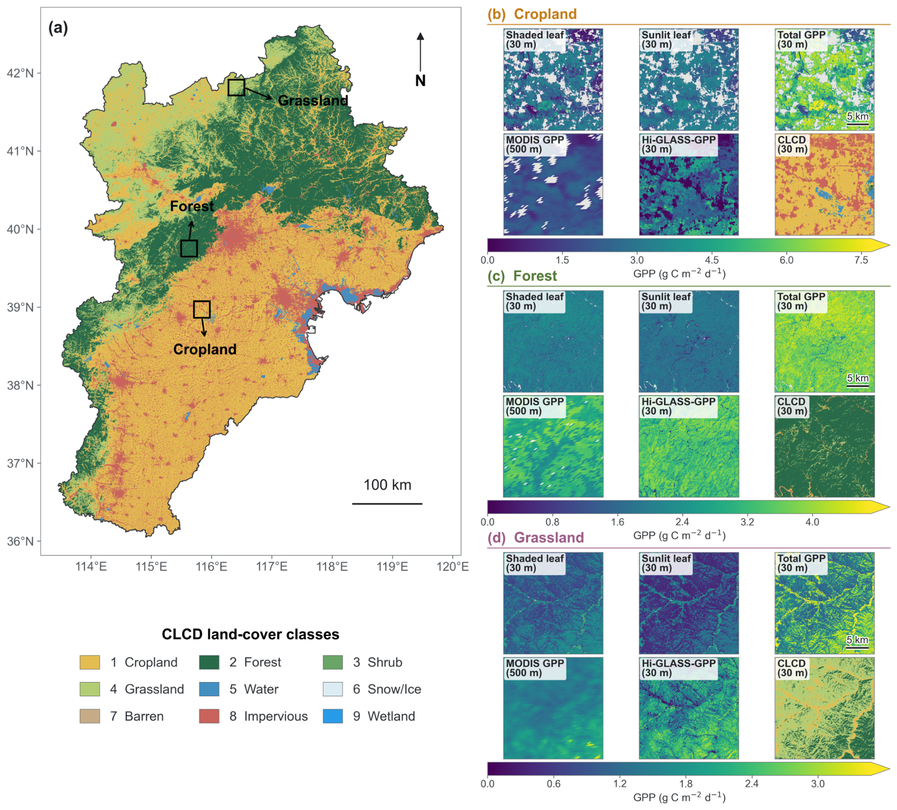
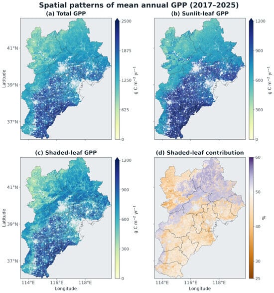
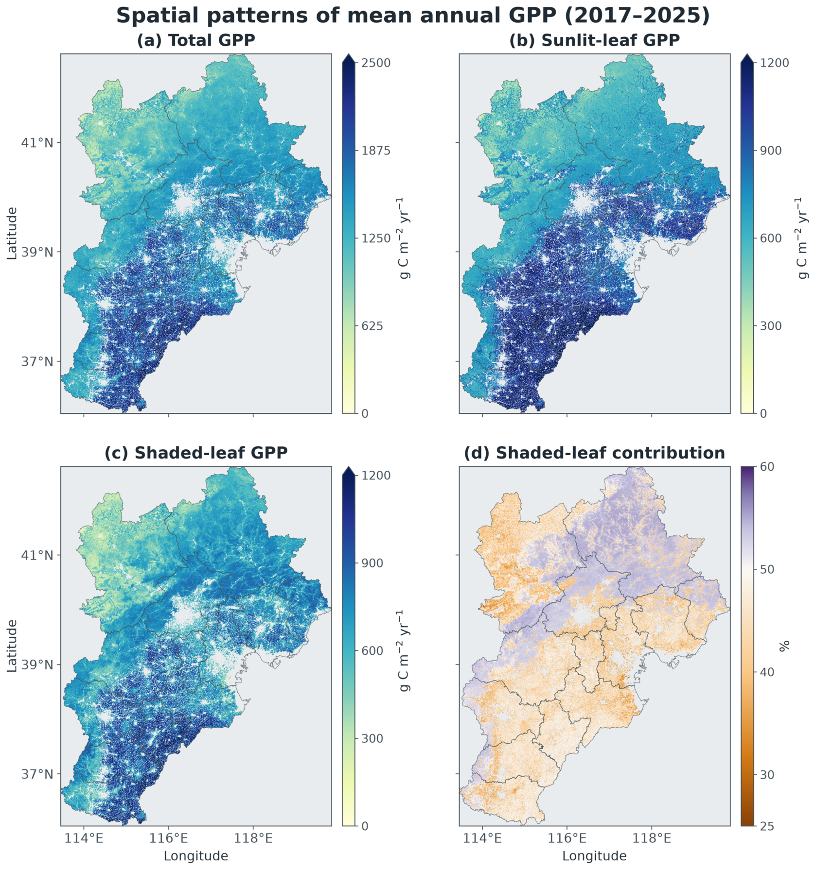
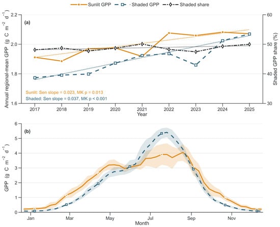
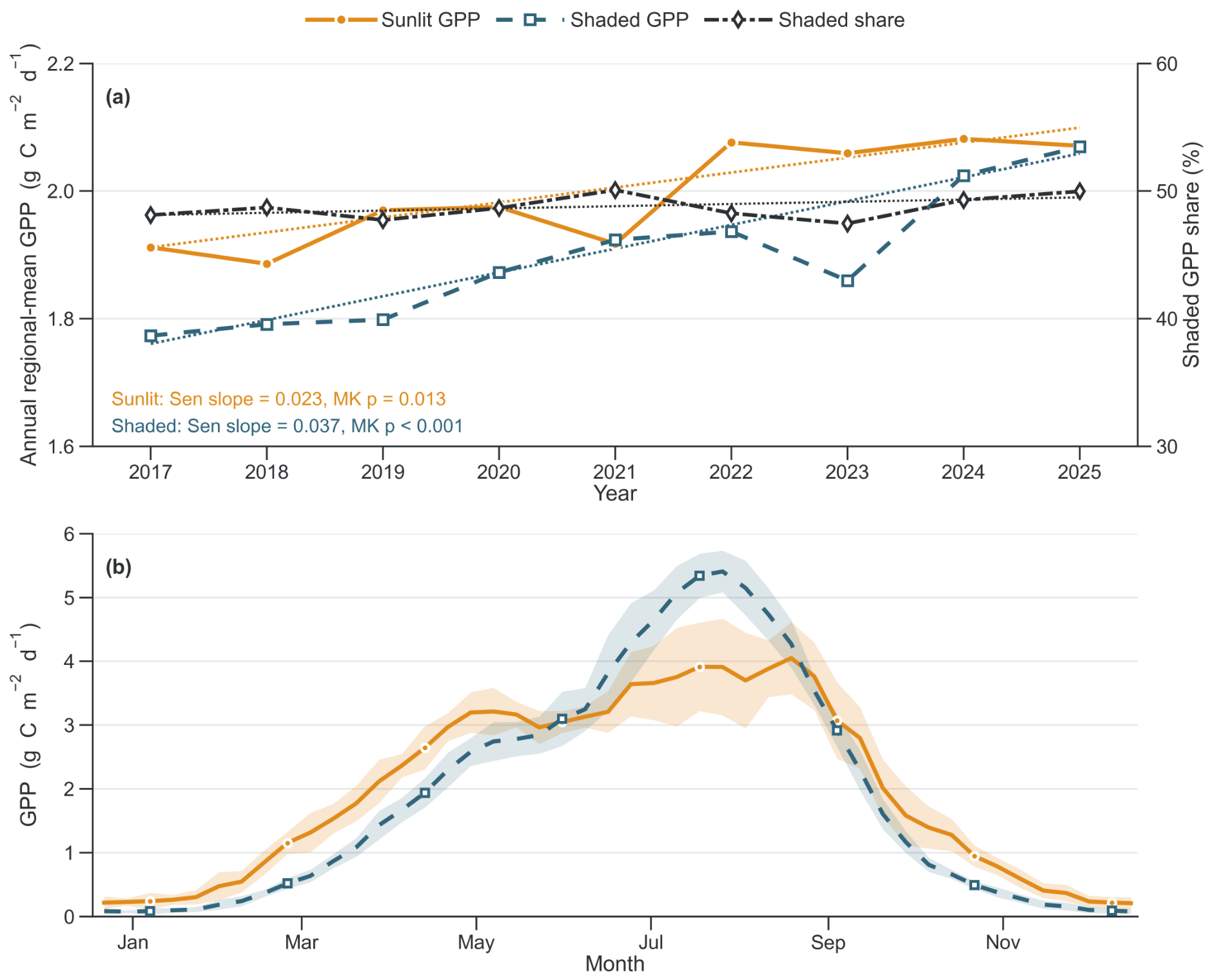
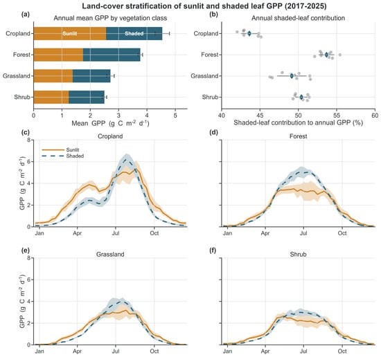
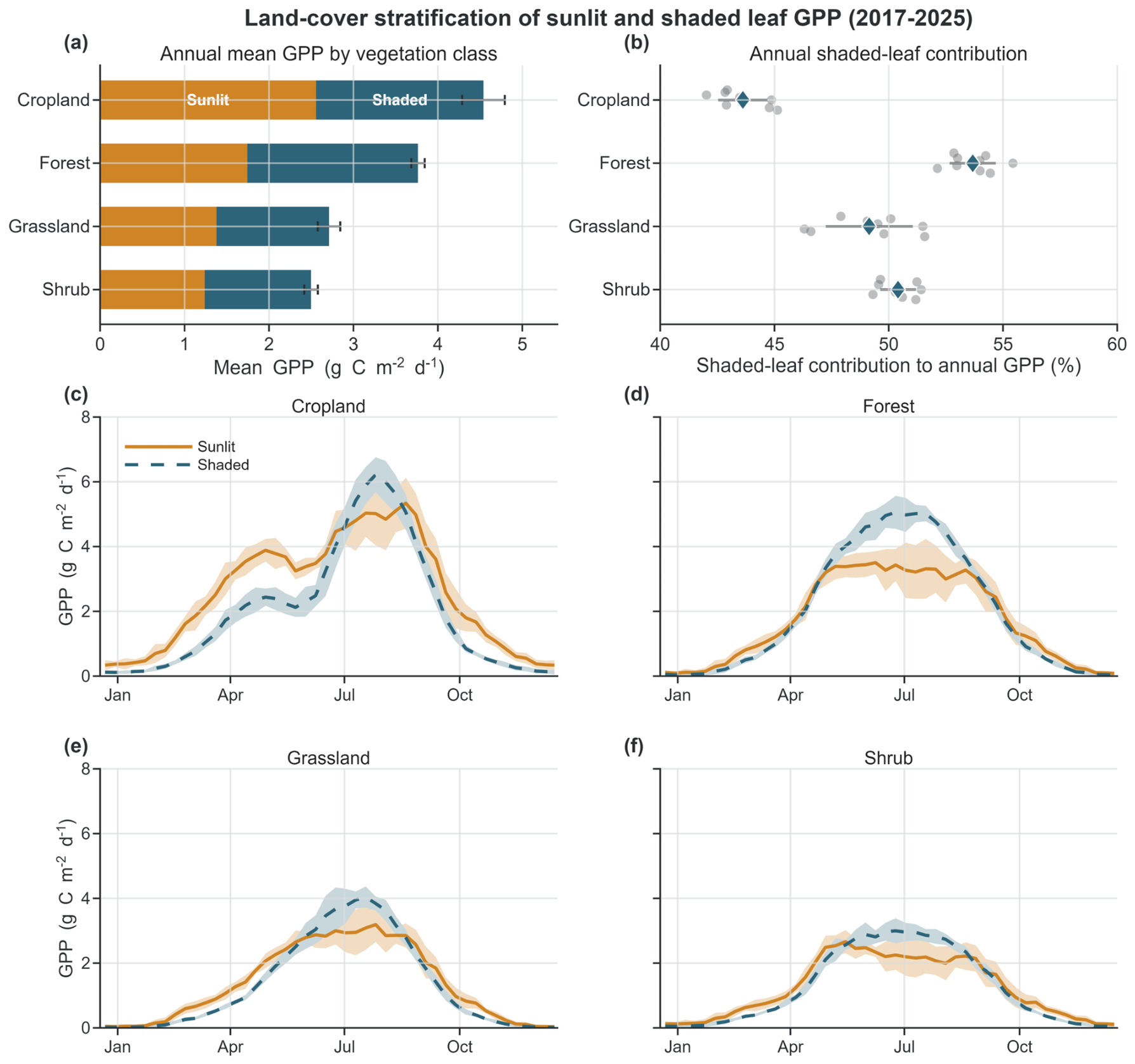
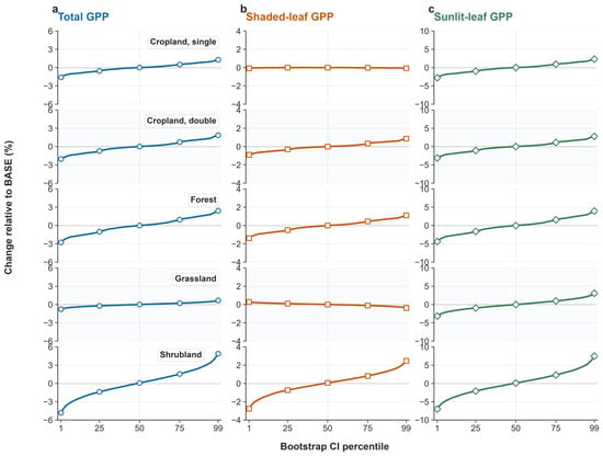
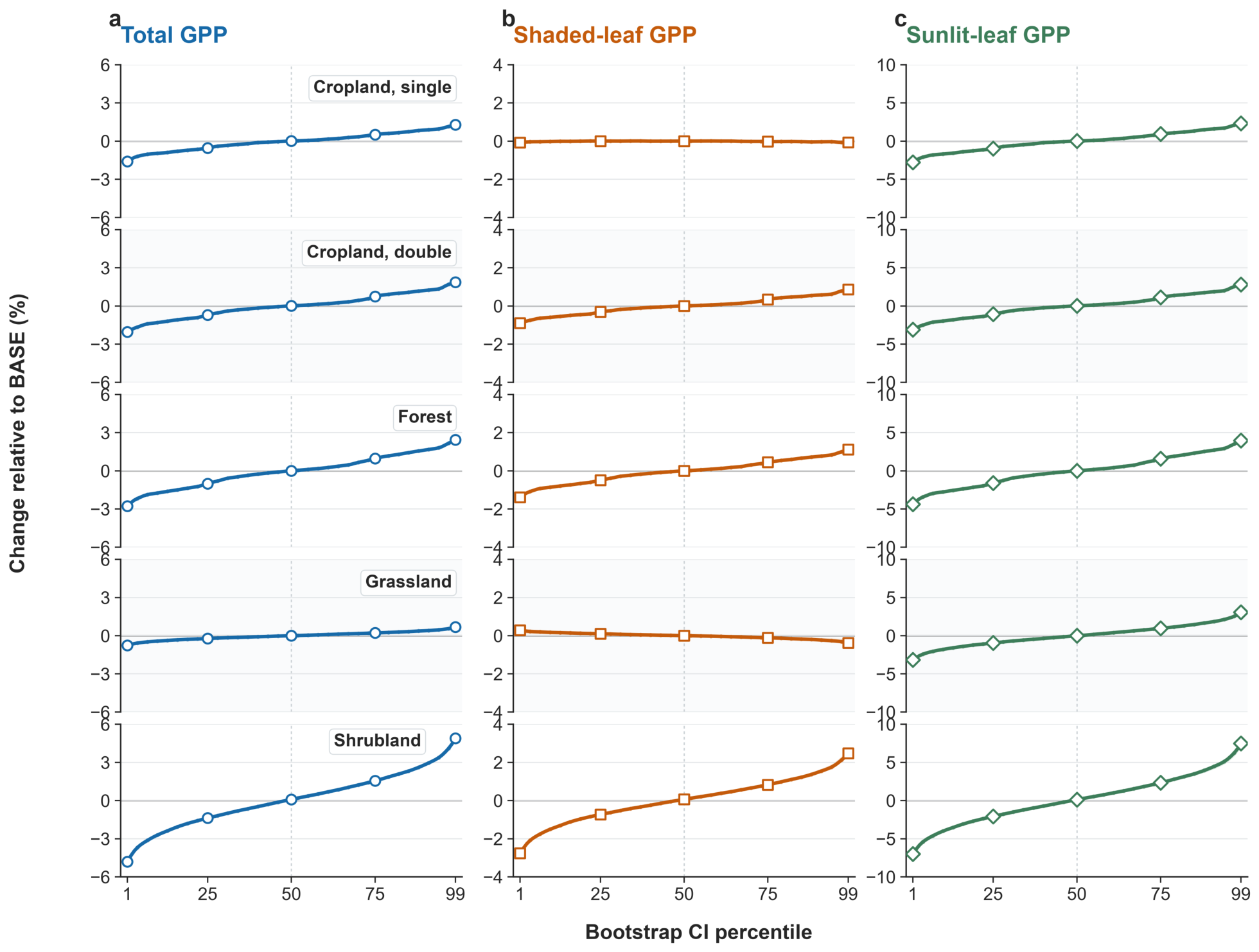

Disclaimer/Publisher’s Note: The statements, opinions and data contained in all publications are solely those of the individual author(s) and contributor(s) and not of MDPI and/or the editor(s). MDPI and/or the editor(s) disclaim responsibility for any injury to people or property resulting from any ideas, methods, instructions or products referred to in the content. |
© 2026 by the authors. Licensee MDPI, Basel, Switzerland. This article is an open access article distributed under the terms and conditions of the Creative Commons Attribution (CC BY) license.