


Highlights
What are the main findings?
- Using a novel approach integrating very high-resolution (0.3–0.5 m) satellite imagery, LiDAR-derived DEMs, and ancillary datasets, we mapped 552 km of irrigation channels, exceeding existing inventories in the study area by 18–35%.
- Constrained dilation and channel connection algorithms extended channel networks beyond areas directly detectable in optical imagery.
- Object-based accuracy assessment demonstrated a low false-positive rate (7.7%), with 76% of newly mapped channels judged to be definite or possible irrigation channels absent from existing inventories.
What are the implications of the main findings?
- The approach can rapidly generate spatially explicit preliminary irrigation channel inventories from input data available across much of the conterminous United States, providing a starting point for production of a comprehensive irrigation channel network inventory.
- Such inventories can support water-resource management, hydrological modeling, and infrastructure planning, particularly in data-sparse regions with limited resources.
Abstract
Comprehensive spatial inventories of irrigation channels inform water-resource management, hydrological modeling, and infrastructure planning, yet remain unavailable for many irrigated regions due to the high cost of manual mapping. Here we present a novel approach for irrigation channel mapping that integrates very high-resolution (0.3–0.5 m) WorldView satellite imagery, 1 m LiDAR-derived digital elevation model data, and ancillary land cover and irrigation datasets. The approach employs a U-Net convolutional neural network and a Hessian filter to identify potential surface-water features from optical imagery, while geomorphon classification identifies potential channel locations from digital elevation model data. A constrained dilation algorithm expands high-confidence channel detections along topographically favorable paths, and an XGBoost classifier distinguishes irrigation channels from natural surface-water features and false positives. Applied to a 569 km2 study area in the San Luis Valley, Colorado, the approach mapped 552 linear kilometers of irrigation channels—18% more than the U.S. Geological Survey National Hydrography Dataset Plus High Resolution and 35% more than the Colorado Division of Water Resources inventory. Object-based accuracy assessment indicated that 92.3% of mapped channel segments were definite or possible irrigation channels, with only 7.7% representing false positives. Among channel segments not appearing in existing datasets, 76% were judged to be definite (43%) or possible (33%) irrigation channels either missed by previous mapping efforts or constructed after the creation of those datasets. While recall (the proportion of reference channel pixels that were correctly mapped) remained limited (0.28), the approach demonstrates potential for rapidly generating spatially explicit channel inventories that provide a starting point for manual refinement: false positives can be removed quickly, whereas adding missed channels requires more substantial effort.
1. Introduction
Irrigation is crucially important for agriculture across the western United States due to the arid or semi-arid climate conditions in the region. Much of the irrigation water derived from rain and snowmelt runoff is delivered to fields via networks of above-ground irrigation channels [1], sometimes also referred to as canals or ditches. These channel networks are managed by a combination of federal and state agencies, as well as local irrigation organizations. While large state- and federally managed channel networks can include hundreds or thousands of kilometers of channels [2,3], smaller irrigation organizations may manage channel networks that include only a few kilometers of channels [4]. For some irrigation districts, comprehensive, detailed maps of irrigation channels are available [5,6]. However, in many others, only large channels delivering water over significant distances or to many recipients have been mapped, while the majority of the channel network has been documented but not explicitly mapped [6,7,8]. In some cases, no formal documentation at all is available for portions of the channel network [5,9,10].
The lack of comprehensive, spatially explicit irrigation channel inventories in some districts reflects the high cost of creating these datasets [5]. Districts or other entities that wish to create a comprehensive, spatially explicit inventory of irrigation channels typically employ some combination of field-based mapping and manual interpretation of high-resolution imagery. Both methods are labor-intensive and can be prohibitively costly. Thus, the introduction of an efficient, effective approach for consistently mapping irrigation channels across large areas has the potential to facilitate the creation of comprehensive irrigation channel maps in regions where they are currently lacking, as well as to ease the burden on agencies and organizations tasked with maintaining and updating existing inventories.
Improving the availability of comprehensive irrigation channel inventories addresses an important data gap and can support effective water-use planning and management [5]. In addition to their direct utility for water-use planning and management, comprehensive, spatially explicit irrigation channel inventories can facilitate more accurate water balance modeling [11,12] and aid in the exploration of the potential for small-scale hydropower projects [13]. High-quality channel inventories also have the potential to serve as the foundation for airborne or spaceborne surface-water monitoring efforts by identifying pixels within the footprint of the channel network for detailed time-series analysis.
Over the last several decades, substantial progress has been made toward the development of remote sensing approaches for mapping surface-water features, resulting in high-quality regional, national, and even global surface-water datasets that are regularly updated [14,15,16,17,18]. In most cases, these surface-water mapping approaches rely heavily on multispectral data, especially multispectral data that includes a middle infrared band [19,20], and is distributed as well-calibrated, atmospherically corrected surface-reflectance data [21,22] that is suitable for discriminating surface water from other surfaces based primarily or entirely on spectral signatures. Most satellite imagery with high enough spatial resolution to resolve irrigation channels does not include a middle infrared band and is not typically distributed as atmospherically corrected surface-reflectance data, hindering the effective use of spectral methods for mapping irrigation channels. Even in very high spatial resolution (<0.5 m) imagery, the area of exposed, visible surface water within the pixel footprint of a typical irrigation channel (1–5 m in width) is often reduced by overlying vegetation. Shadowing from taller vegetation, buildings, and even the sides of the channel itself can also alter the spectral signature of surface water in the channel. These effects result in mixed pixels, which are far more difficult to classify than pure pixels based on spectral signatures alone [23,24,25].
More recently, optical remote sensing approaches have increasingly relied on computer vision techniques that consider not only the spectral signature of pixels, but also the arrangement of those pixels [26]. These techniques, which include deep learning methods, have been applied to map a wide variety of features from satellite imagery that could not be reliably identified from spectral signatures alone [27]. Over the same period, new approaches have been developed to identify surface-water features from high-resolution (<2 m) digital elevation model (DEM) data [28,29,30,31], often by incorporating deep learning algorithms like those recently adopted for use in optical remote sensing.
Relatively few studies have addressed the automated extraction of artificial channels such as irrigation canals and drainage ditches specifically. Most existing work has focused on drainage ditches, which have been mapped from high-resolution LiDAR-derived DEMs using topographic analysis and rule-based or semi-automatic methods in flat agricultural landscapes [28,29,30,32], and more recently using supervised machine learning and deep learning approaches [33,34,35]. These DEM-based approaches can detect narrow ditches that are difficult to identify in optical imagery, but they characterize channel form rather than function. Distinguishing artificial ditches from natural streams with similar morphology remains challenging [35], and DEM data alone provide little information on whether a channel is in active use. Some studies have addressed these limitations by integrating DEM data with additional information, such as LiDAR intensity to identify channels containing water [36], or aerial optical imagery combined with LiDAR derivatives as inputs to a deep learning classifier [37]. Studies focused specifically on irrigation canals are fewer still. Canals have been mapped from very high-resolution imagery acquired by unmanned aerial vehicles (UAVs) using object-based and deep learning methods [38,39], but these approaches have been demonstrated only over small areas, and the narrowest canals remained difficult to detect even at UAV resolution [38]. At a regional scale, canal networks have been mapped from 3 m PlanetScope imagery and DEM data using a graph-constrained semantic segmentation approach trained on existing hydrography data [7], though the moderate resolution of the imagery likely limits the detection of narrow lateral channels. A global registry of irrigation canals has also recently been compiled from OpenStreetMap data, using a classifier to separate canals from natural rivers [40], but such inventories depend on the completeness of existing volunteered or agency mapping. Together, these studies highlight several persistent challenges for automated irrigation channel mapping: the narrow width of many channels relative to image resolution, obscuration by vegetation and shadow, discrimination between artificial and natural channels, discontinuities in mapped networks, and the need to identify channels that are in current use.
In this paper, we describe a novel approach that maps irrigation channels using a combination of very high spatial resolution (0.3–0.5 m) satellite imagery, DEM data, and existing land cover and irrigation datasets. Although numerous sophisticated digital terrain analysis methods for extracting natural surface-water networks from DEM data have been extensively investigated (e.g., [41,42,43,44,45,46]), these techniques are generally ill-suited for delineating artificially constructed channel networks. To address this limitation, we employ a hybrid approach that integrates machine learning classification algorithms with rule-based heuristics to first identify prominent surface-water channels using both satellite imagery and DEM data and subsequently extend and connect these features to construct a more comprehensive representation of the irrigation channel network.
The very high-resolution satellite imagery and high-resolution LiDAR-derived DEM data that our approach relies on are now available across much of the conterminous United States, while the existing land cover and irrigation data we use are available across the entire conterminous U.S. The approach we present ingests these datasets, applies a series of raster and vector processing algorithms, and outputs a vector dataset of irrigation channels that can serve as a starting point for manual refinement prior to incorporation into planning and analysis workflows. We used manually edited geospatial data from the study area to calibrate the approach and assess its accuracy.
2. Methods
2.1. Study Area
The study area is located in the San Luis Valley, a large (~8000 km2) mountain valley in south-central Colorado, USA, situated between the San Juan Mountains to the west and the Sangre de Cristo Mountains to the east. The study area is defined by a 17.55 × 32.40 km rectangle (Figure 1), covering a 569 km2 region immediately to the south of the Rio Grande, which flows from west to east across this portion of the valley. The mean elevation of the study area is 2342 m, with flat or gently sloping terrain throughout. A substantial portion of the study area consists of irrigated cropland dominated by alfalfa and barley [47]. We selected the study area based on the high concentration of irrigation channels in the region as well as the availability of suitable WorldView imagery and U.S. Geological Survey (USGS) 3D Elevation Program (3DEP) LiDAR-derived 1 m DEM coverage.
Figure 1.
Map of the San Luis Valley, CO, USA, with study area extent (solid black line) and accuracy assessment subset regions enumerated and surrounded with dashed black line, overlaid on the National Land Cover Database 2021 land cover layer.
2.2. Data
2.2.1. Very High-Resolution Satellite Imagery
We acquired orthorectified multispectral and panchromatic data for six WorldView-3 [48] and three WorldView-2 [49] scenes (hereafter, WorldView scenes) covering a portion of the study area that met several key criteria, including seasonality, recency, cloud cover, resolution, and view geometry. Only scenes that met all of the following criteria were acquired: (1) scene acquisition date was between April 20 and September 10 (seasonality), (2) scene acquisition year was 2015 or later (recency), (3) the scene included at least one region of contiguous cloud-free imagery >9 km2 within the study area based on the initial visual assessment (cloud cover), (4) panchromatic spatial resolution was ≤0.55 m (resolution), and (5) view zenith angle was ≤25 degrees off-nadir (view geometry).
2.2.2. USGS 3D Elevation Program (3DEP) LiDAR-Derived Digital Elevation Model Data
Digital elevation model (DEM) data at 1 m spatial resolution were acquired for the full extent of the study area from the USGS National Map 3DEP Downloadable Data Collection [50]. The 3D Elevation Program (3DEP) is a national initiative led by the USGS to provide high-resolution three-dimensional elevation data for the conterminous U.S., Hawaii, Alaska, and U.S. territories [51]. The 1 m DEM product is the highest-resolution standard DEM in the 3DEP product suite and is derived exclusively from LiDAR point cloud data with a density of ≥2 pulses/m2, with accuracy specified as ≤10 cm root mean square error for non-vegetated surfaces (RMSEz) [51,52]. The data for this study area are projected to Universal Transverse Mercator (UTM) Zone 13 North and referenced to the North American Datum of 1983 (NAD 83) for horizontal positioning, while all 3DEP 1 m DEM data are referenced vertically to the North American Vertical Datum 1988 (NAVD 88), with elevation values reported in decimal meters [50]. The vertical accuracy of the DEM may be reduced in areas with dense vegetation canopy, where LiDAR pulses may not fully penetrate to the ground surface [53,54].
2.2.3. Ancillary Data
We compiled several ancillary spatial data layers, including both raster and vector spatial datasets. Raster datasets included tiled data for the study area from the most recent United States Department of Agriculture’s National Agriculture Imagery Program (NAIP) [55], the National Land Cover Database (NLCD) 2021 land cover classification [56], the NLCD 2021 impervious surface classification [57], the NLCD 2021 forest canopy classification [58], and the LANID land irrigation data layers available for 2000–2020 [59]. Vector datasets included the USGS National Hydrography Dataset Plus (NHD+) High Resolution [60] and a dataset of irrigation channels mapped by the Colorado Division of Water Resources (DWR) [61].
2.3. Image Processing and Channel Network Extraction
Our approach implements a series of processing steps that transform the input datasets (Table 1) into a vector database of irrigation channels segmented into reaches with lengths of approximately 25 m each (Figure 2). The core of our approach relies on the combination of surface-water classification from very high-resolution imagery and digital terrain analysis for extraction of channels from DEM data. While digital terrain analysis methods for extracting natural surface-water networks from DEMs have been extensively investigated [41,42,43,44,45,46], these techniques are generally ill-suited for delineating artificially constructed channel networks. To address this limitation, our approach relies on a novel combination of machine learning algorithms and simple rules to identify prominent surface-water features that can be derived independently from both very high-resolution optical imagery and DEM data. These core surface-water features are subsequently extended and connected to construct a more comprehensive representation of the irrigation channel network.
Table 1.
Datasets used in this study. Abbreviations used are listed below.
Figure 2.
Schematic diagram of processing approach. Processing steps are grouped into four stages and labeled with the section of the manuscript in which each is described. The dashed arrow indicates that per-polygon summary metrics computed from the input raster stack are used by the object-based classifier. Acronym definitions: WorldView (WV), WorldView-2 (WV2), WorldView-3 (WV3), National Agriculture Imagery Program (NAIP), digital elevation model (DEM).
Here we provide a high-level overview of the processing steps, with detailed descriptions of each step provided in Section 2.3.1, Section 2.3.2, Section 2.3.3, Section 2.3.4, Section 2.3.5, Section 2.3.6, Section 2.3.7, Section 2.3.8, Section 2.3.9 and Section 2.3.10. First, WorldView imagery is pan-sharpened and registered to NAIP imagery using a phase cross-correlation (PCC) approach (Figure 2, Section 2.3.1), and then composited to form a seamless, cloud-free mosaic covering the entire study area (Figure 2, Section 2.3.2). Derivative layers are computed from DEM data (Figure 2, Section 2.3.3) as well as from the ancillary raster datasets (Figure 2, Section 2.3.4). The imagery mosaic, DEM and derivatives, as well as the ancillary datasets and their derivative layers are resampled to a 0.3 m raster to facilitate further processing. A convolutional neural network (CNN) and a Hessian filter are applied to the WorldView imagery to identify potential surface-water features (Figure 2, Section 2.3.5), while a geomorphological classification approach is separately applied to the DEM data to identify potential channel features (Figure 2, Section 2.3.6). We then intersect the potential surface-water raster derived from WorldView imagery and the potential channels raster derived from the DEM to identify a subset of high-confidence surface-water channel features. The high-confidence surface-water raster is used to “grow” channels constrained by topography to fill out the remainder of the channel network (Figure 2, Section 2.3.7). Summary metrics (mean, maximum, and minimum) are computed for the DEM layer and its derivatives, as well as for each ancillary data layer, for regions of contiguous pixels identified from the updated channels raster image. The summary metrics and additional shape-based metrics are then provided as the input to a gradient-boosting tree algorithm that classifies each contiguous region as a natural surface-water feature, irrigation channel network feature, or false positive (Figure 2, Section 2.3.8). We then apply a post-processing algorithm to the classified regions that uses a rules-based approach to connect nearby regions when certain criteria are met (Figure 2, Section 2.3.9). Finally, elongated regions classified as irrigation channels and meeting a minimum length threshold are segmented into reaches of approximately 25 m in length to facilitate further analysis (Figure 2, Section 2.3.10). The design and implementation of accuracy assessment approaches are described in Section 2.3.11.
Although each step is described separately below, the steps are designed to work together as a sequence, with each step operating on the output of the preceding step and addressing a specific limitation of the steps before it (Figure 2). The union of the U-Net and Hessian filter outputs is intentionally permissive, detecting many narrow channels at the cost of numerous false positives. Intersecting this classification with the DEM-derived potential channels is intentionally strict, retaining only pixels supported by both data sources, but capturing only fragments of the channel network. Constrained dilation then extends these high-confidence fragments along topographic lows, the object-based classifier distinguishes irrigation channels from natural surface-water features and removes remaining false positives, and the connection step closes gaps that remain in the network. Because of this interdependence, none of the intermediate products is a usable map of irrigation channels on its own; the DEM-derived classification, for example, includes valley and depression landforms regardless of whether they carry water. The parameters and thresholds used in each step, the basis for their selection, and their expected effects are summarized in Table 2.
Table 2.
Parameters and thresholds used in the processing workflow, the basis for their selection, and the expected effect of increasing each value. Settings used to train the U-Net and XGBoost classifiers are given in Section 2.3.5 and Section 2.3.8. Pixel (px) values refer to the 0.3 m processing grid unless otherwise noted. Abbreviations: DFMLE, difference from mean local elevation; HOT, Haze Optimized Transformation; NIR, near infrared.
2.3.1. Image Preprocessing
We completed several preprocessing steps to pan-sharpen the WorldView imagery and spatially register the imagery to the DEM prior to the construction of a seamless cloud-free composited mosaic covering the entire study area. Pan-sharpening is an approach that uses higher spatial resolution panchromatic band data to sharpen lower spatial resolution multispectral bands [62]. While several different pan-sharpening approaches are available, use of a deep learning approach to implement pan-sharpening has been shown to produce superior results [63]. We used the Zoom Pan-sharpening Neural Network (Z-PNN) approach [64], which employs a convolutional neural network (CNN) to implement pan-sharpening across all the available WorldView scenes that were used to build the seamless cloud-free image composite (described in Section 2.3.2). The final resolution of pan-sharpened imagery matched the resolution of the panchromatic imagery for each WorldView scene and varied from 0.31 m to 0.55 m.
Visual assessment of the available WorldView scenes overlaid with the DEM data indicated misregistration between the two different datasets, with offsets > 4 m from the DEM apparent for some WorldView scenes. Visual assessment of the most recent available multispectral NAIP imagery from 2023 indicated the NAIP imagery was more precisely registered to the DEM data than the WorldView imagery. For each WorldView scene, we registered the WorldView imagery to the NAIP imagery by resampling the WorldView scene data to match the projection and resolution of the 0.3 m resolution NAIP imagery, dividing the WorldView scene into 250 × 250 pixel registration tiles, and applying a PCC algorithm [65] to compute x and y pixel offsets for the WorldView red spectral band from the NAIP red spectral band. This improved registration of the WorldView imagery to the DEM data, with computed pixel offset values for most registration tiles in the single digits and within two pixels of the corresponding pixel offset values from adjacent registration tiles. For cases where computed offset values exceeded 15 pixels in one or both dimensions, or computed offset values differed from the 5 × 5 tile neighborhood mean by more than two pixels, the x and y pixel offset values for the tile were replaced with the mean x and y offset values for the neighborhood (recomputed after exclusion of any tiles with out-of-range values). Once valid x and y offset values were established for the entire set of registration tiles for the WorldView scene, the offsets computed from the red band for each registration tile were applied to all WorldView spectral bands across the entire set of registration tiles, resulting in WorldView imagery that was more precisely registered to the NAIP and DEM raster data.
2.3.2. Construction of Seamless Cloud-Free Image Composites
We designed our processing pipeline to be suitable for mapping irrigation channels across regions much larger than the extent of a single WorldView scene. Compositing of WorldView scenes acquired on multiple dates, at a variety of spatial resolutions and at a range of view zenith angles, was necessary to cover the full extent of the study area. To facilitate parallel processing and reduce the amount of memory required for processing, we divided the study area into 1.5 × 1.5 km (5000 × 5000 pixel) image processing tiles. We used a 500-pixel overlapping tile scheme that ensured that edge regions within an image processing tile that could not be fully processed by algorithms considering a neighborhood size up to 500 pixels would be fully processed in the adjacent image processing tile, resulting in complete coverage (excluding the edges of the study area). Subdividing the 17.55 × 32.40 km study area using this tiling scheme resulted in a grid of 13 × 24 image processing tiles.
A seamless, cloud-free composite mosaic was generated across the full spatial extent of the study area using a hierarchical tiling approach with pixel-level quality assessment. Each image processing tile (5000 × 5000 pixels) was subdivided into 100 compositing subtiles of 500 × 500 pixels, and compositing suitability scores were computed for each compositing subtile for the corresponding spatial extent of each available WorldView scene. The compositing suitability metric was designed to rank overlapping WorldView acquisitions based on three criteria: (1) valid data coverage (0–100%), (2) cloud contamination probability (0–100%), and (3) similarity to NAIP reference imagery (correlation value between 0 and 1). The inclusion of NAIP similarity served as a proxy for detecting either landscape change occurring between WorldView and NAIP acquisition dates (the latter being invariably more recent) or residual contamination from undetected cloud cover or cloud shadows.
Valid data coverage was quantified at the pixel level, with pixels classified as invalid when the digital number (DN; the raw, uncalibrated sensor value) equaled zero in three or more of the eight spectral bands. The coverage metric was calculated as the percentage of pixels exhibiting DN values greater than zero in at least six bands relative to the total pixel count within each compositing subtile.
Cloud probability was estimated for individual pixels within each WorldView scene using a weighted ensemble of four spectral indices. A brightness index was calculated as the mean normalized reflectance across all spectral bands, exploiting the characteristically elevated and uniform reflectance of clouds throughout the visible and near-infrared spectrum [66]. A whiteness index quantified spectral flatness by measuring the deviation of individual visible band reflectances from their mean, capitalizing on the achromatic signature characteristic of optically thick clouds [67]. The Haze Optimized Transformation (HOT), computed as the difference between blue and red band reflectance [68], was applied to detect thin clouds and atmospheric haze. Finally, the ratio of near infrared (NIR) to visible reflectance was employed to discriminate clouds from spectrally bright vegetation, which exhibits characteristically elevated NIR reflectance. These indices were integrated into a composite cloud probability score using empirically determined weights (brightness: 0.35; whiteness: 0.35; HOT: 0.20; NIR ratio: 0.10). The compositing subtile-level cloud probability was subsequently computed as the mean of pixel-level cloud probability values, with potential values ranging from 0 to 100.
Similarity to NAIP reference imagery was assessed by computing the Pearson correlation coefficient between red band reflectance values of spatially corresponding pixels from the WorldView and NAIP datasets. To facilitate computation of the final weighted scores, correlation coefficient values <0 were set to zero, and the correlation coefficient values were then multiplied by 100, resulting in a range of potential NAIP similarity scores from 0 to 100.
The final composite mosaic was constructed by populating each compositing subtile with spectral band data from the WorldView scene exhibiting the highest suitability score for that compositing subtile. An example of the cloud-free, composited WorldView mosaic is shown in Figure 3.
Figure 3.
Example of a seamless, cloud-free, 0.3 m, 8-band image composite produced by automatic selection of the best cloud-free imagery available for each compositing subtile. Substantial differences in vegetation phenology are evident (with reddish tones indicating croplands prior to harvest and dull grey and brown tones indicating croplands after harvesting) along subtile boundaries, which are indicated by dashed lines. Despite these differences, the irrigation channel remains distinctly visible and continuous at the locations where it crosses the subtile boundaries, which are circled in yellow.
2.3.3. Computation of Topographic Derivatives
Two types of raster derivative layers were computed from the 1 m DEM: (1) slope and (2) difference from mean local elevation (DFMLE). The single slope derivative layer was computed using a 5 × 5 pixel neighborhood with the third-order bivariate Taylor polynomial method described in [69]. Three separate DFMLE raster layers were computed from the DEM, after feature-preserving smoothing with an 11 × 11 pixel filter, using local neighborhoods of 15 × 15 pixels, 99 × 99 pixels, and 999 × 999 pixels.
2.3.4. Computation of Additional Ancillary Data Derivatives
Ancillary datasets described in Section 2.2.3 were used to compute derivative layers designed to provide contextual information on local land cover and irrigation characteristics from 30 m Landsat data (Table 1). For the 30 m National Land Cover Database (NLCD) land cover data layer, we computed derivative layers indicating the fraction of water, barren, shrub, grassland, pasture/hay, cultivated crops, herbaceous wetlands, and woody wetlands in a 7 × 7 pixel (210 × 210 m) window surrounding each pixel. Rather than computing neighborhood fraction values for the urban/impervious and forest classes, we computed mean impervious fraction and mean forest fraction from the separate NLCD impervious and NLCD forest canopy layers, which provide more detailed information on each land cover type. Recognizing the relative importance of the neighborhood fraction of cultivated crops, we also computed cultivated crop fraction for a larger 31 × 31 pixel (930 × 930 m) window. For the LANID irrigated extent dataset, we computed the maximum irrigated fraction (over the period 2000–2020) for 7 × 7 pixel (210 × 210 m) neighborhoods and 31 × 31 pixel (930 × 930 m) neighborhoods. While the horizontal resolution (Table 1) varied between ~1 × 1 m and 930 × 930 m, all data were resampled to the same 0.3 m grid as the WorldView imagery composite using nearest-neighbor interpolation.
2.3.5. Image-Derived Potential Surface-Water Feature Classification
Classification of potential irrigation channels in WorldView imagery was accomplished through a hybrid approach employing a U-Net convolutional neural network [70] in conjunction with a Hessian-based filter [71] applied to a weighted grayscale combination of the green, red, and near-infrared 2 bands of the WorldView imagery. The final classification was derived from the union of outputs from both methods. The U-Net classifier was trained using data extracted from 12 WorldView scenes acquired during spring and summer months across irrigated agricultural regions in Colorado, Montana, and Idaho. Subset images containing features of interest from each WorldView scene were carefully segmented and labeled using a hybrid approach that included manual inspection and quality assurance. The labeled subsets were divided into image tiles, 40% of which were randomly reserved for validation so that training and validation data were drawn from non-overlapping areas. The U-Net classifier was trained and implemented on 128 × 128 image subsets, referred to hereafter as chips. Chips were extracted from each tile on a regular grid with a 32-pixel stride, and each chip was buffered by 32 pixels on each side (192 × 192 pixels) so that geometric augmentations (e.g., rotation or shear) could be applied without the need for padding. Each image chip was composed of 8 bands of spectral data from WorldView imagery along with a corresponding binary mask identifying the extent of surface water across the 192 × 192 pixel chip. Chips with little or no surface water were subsampled to reduce class imbalance.
To increase training sample size and improve model generalization, up to four augmented versions of each training chip were added to the training dataset, with more versions generated for chips containing a larger proportion of surface water. Each augmented version was generated using one of 11 randomly selected augmentation sequences combining rotation by 10–35° in either direction, horizontal reflection, shear of up to 20° along one or both image axes, brightness adjustment of 3–7%, random dropout of 1–4% of pixels, and additive Gaussian noise (standard deviation of 3–9% of the 8-bit data range), with dropout and noise applied independently to each spectral band. Additionally, a 3 × 3 pixel maximum filter was applied to the surface-water reference masks prior to chip extraction, expanding the surface-water class by one pixel to account for uncertainty in the precise delineation of land-water boundaries. The final training dataset for the U-Net model was constructed by extracting the 128 × 128 pixel chip at the center of each original and augmented 192 × 192 pixel chip. Validation chips were extracted from the validation tiles using the same procedure, but without augmentation.
The U-Net was implemented in TensorFlow/Keras version 2.9.0 using the Segmentation Models library [72], with a ResNet-34 encoder [73] initialized with weights pretrained on the ImageNet dataset [74]. Because the pretrained encoder expects three input channels, the eight WorldView bands were first passed through a trainable 1 × 1 convolutional layer that mapped them to three channels. The network produced per-pixel probabilities for two classes (land and surface water) using a sigmoid output activation. The model was trained with the Adam optimizer (learning rate of 5 × 10⁻⁶) to minimize binary cross-entropy loss, using a batch size of 256 and a maximum of 500 epochs, with training stopped early when the validation loss failed to improve for five consecutive epochs. Training stopped after 68 epochs, and the weights from epoch 63, which had the lowest validation loss, were retained.
Although irrigation channels with widths as narrow as 60 cm were discernible in the WorldView imagery, the U-Net classifier exhibited limited skill in detecting these narrow linear features. To address this limitation, the Hessian filter was implemented to identify additional dark, linear structures within the imagery. The Hessian filter was implemented using the skimage package [75], with scales (σ) of 1, 3, 5, 7, and 9 pixels, alpha, beta, and gamma parameters of 1.0, 0.5, and 50, respectively, and the black_ridges option set to False.
The final potential surface-water classification product was generated by computing the union of the U-Net-derived surface-water classification (pixels with a predicted surface-water probability >0.25) and the Hessian filter output, from which isolated regions of fewer than 250 contiguous pixels had first been removed with a sieve filter. To exclude detections outside topographic lows, the union was then restricted to pixels with DFMLE values for the 15 × 15 pixel neighborhood (DFMLE15) <−0.15 m, after expanding this mask by three pixels to retain channel margins. The selection of the 250-pixel sieve threshold was based on visual assessment of initial results suggesting that most features with fewer than 250 contiguous pixels did not represent true surface-water features.
2.3.6. DEM-Derived Potential Channel Classification
To delineate potential channel features from the DEM, the 1 m resolution DEM was classified into discrete geomorphological landform elements (geomorphons) following the pattern recognition methodology described in [76]. Geomorphons were computed from the smoothed DEM (Section 2.3.3) using a 31 m search radius, a 3 m skip radius, and flatness thresholds of 2° (strict) and 1° (relaxed). Pixels classified as valleys or depressions with the strict threshold were treated as potential channels. Pixels classified as flat or hollow, pixels classified as valleys or depressions only with the relaxed threshold, and the outer three pixels of all other landforms were treated as transitional. Potential channels were expanded into transitional pixels by three iterations of dilation with a 3 × 3 kernel, resampled to the 0.3 m grid, dilated by a further five iterations, and filtered to remove regions of fewer than 6500 pixels. The resulting regions were then narrowed by iterative erosion with a 3 × 3 kernel (up to 24 iterations, applied within 32 × 32 pixel windows), stopping before erosion would split a region, to produce a binary raster of potential channel locations.
2.3.7. Integration of Image-Derived and DEM-Derived Classifications and Application of Constrained Dilation
Computing the intersection of the image-derived potential surface-water features and the DEM-derived potential channels identified the pixels most likely to represent surface-water channels. Visual evaluation of the resulting raster alongside the WorldView imagery composite and DEM data suggested that this set of pixels covered only a small fraction of the total surface-water channels on the landscape.
To capture a more complete representation of surface-water channels, we developed an approach to use the high-confidence surface-water channels raster as a seed image to grow channels, constrained by the local topography. We created a mask image representing pixels with DFMLE15 values <−0.2 m. The difference threshold of 0.2 m, which represents twice the stated vertical accuracy of the DEM product, was selected to minimize the impacts of noise on the resulting mask. We then iteratively dilated the surface-water channel raster using a 3 × 3 kernel for 60 iterations, retaining only added pixels within the mask, and then removed regions of fewer than 500 contiguous pixels with a sieve filter.
2.3.8. Object-Based Channel Type Classification and False Positive Identification
The raster data image resulting from application of the constrained dilation approach in Section 2.3.7 was converted to a polygon dataset to facilitate further refinement using an object-based classification approach based on a combination of spectral characteristics derived from the WorldView image composite (dataset 3 in Table 1), including selected spectral bands and the normalized difference vegetation and water indices, the surface-water probability output by the image classification (Section 2.3.5), topographic information derived from the DEM (datasets 5–9 in Table 1), and land cover, impervious surface, forest canopy, and irrigation context (datasets 10–26 in Table 1), as well as 12 shape metrics computed using the measure.regionprops function in the Python library scikit-image version 0.19.2 [77]. The shape metrics computed included area, area of the bounding box, convex area, filled area, major axis length, minor axis length, eccentricity, equivalent diameter area, extent, orientation, perimeter, and solidity. To create the training dataset for the object-based classification, we labeled a subset of the polygon features, categorizing each feature as a natural surface-water feature, an irrigation channel, or a false positive (non-water) feature. The final training dataset comprised 569 labeled polygons: 34 natural surface-water features, 171 irrigation channels, and 364 false positives. This dataset was used to train an XGBoost gradient boosting classifier [78], which was then applied to the full set of polygons. The classifier was implemented with XGBoost (version 2.1.4) as a three-class model using the multi-class softmax objective, with 600 boosting rounds, a maximum tree depth of 8, a learning rate of 0.05, row and column subsampling rates of 0.8, and histogram-based tree construction; all other parameters were left at their default values. Each polygon was described by 93 input features: the 12 shape metrics and 81 summary statistics (the minimum, maximum, and mean of 27 spectral, topographic, land cover, and irrigation layers). All 569 labeled polygons were used to train the final model, and no polygons were withheld for validation; the accuracy of the final channel network was instead evaluated independently using the pixel-based and object-based accuracy assessments described in Section 2.3.11. Following classification, objects assigned to natural surface water or irrigation channel classes were retained with their associated class labels, whereas objects classified as false positives were excluded from subsequent analysis. The resultant vector dataset comprised channel features identifiable through the integration of high-resolution multispectral imagery and digital elevation model data.
2.3.9. Connection of Nearby Channels
We developed an additional approach to fill in gaps in the channel network that may not have been addressed with the constrained dilation approach. The approach was designed to make connections between nearby polygons when certain key criteria were met. We computed the isoperimetric quotient, a measure of compactness, for each polygon and identified features with values <0.2 as candidates for connection with other polygons. For each candidate polygon, we selected potential connection points, hereafter referred to as origin points, by computing endpoints along the major axis of the polygon. Potential connection lines were constructed by computing line length and orientation between the origin point and endpoints from other polygons within a 60 m radius of the origin point, excluding any polygons oriented parallel to the origin polygon. Connection lines ≤10 m in length were implemented between the origin point and all endpoints from other polygons. Connection lines longer than 10 m were only implemented if the orientation of the potential connection line was within ±15° of the major axis of either the origin polygon or the polygon to be connected and the orientations of the two polygons to be connected were within an allowed tolerance that varied by line distance. The tolerance value for polygon orientation was ±45° for connection distances of 11–20 m, ±25° for connection distances of 21–35 m, and ±15° for connection distances of 36–60 m. Connection lines between an origin polygon and a destination polygon that intersected a third polygon were prohibited for all distances. Finally, once a connection line was implemented, a connection polygon was constructed by buffering the connection line at a distance of 0.75 m. The connection polygons were added to the original polygon dataset.
2.3.10. Segmentation of Channel Features and Computation of Channel Length and Width
To facilitate further analysis, such as the computation of total channel length or mean channel widths over regular intervals, we developed an approach to merge and then subdivide the existing mapped irrigation channel features into similarly sized segments analogous to reaches in a stream network.
First, we aggregated all polygons classified as irrigation channels, followed by boundary dissolution within each spatially contiguous feature cluster using the geopandas Python package version 0.13.2 [79]. This operation eliminated artificial internal boundaries arising from image processing tile-edge artifacts while preserving the geometric distinctness of non-adjacent channel segments. To avoid subdividing features such as ponds or small, isolated channel fragments, only features in the dissolved polygon dataset classified as irrigation channels with major axis length >50 m and a compactness index <0.2 were eligible for segmentation.
Each qualifying dissolved feature was segmented individually using an axis-oriented slab decomposition algorithm, as described in [80] and implemented using the shapely Python package version 2.1.0 [81]. In this approach, a polygon is divided into parallel rectangular strips (“slabs”) of fixed maximum width along a reference axis. First, each polygon was rotated so that its longest dimension (the major axis of its minimum bounding rectangle) was aligned horizontally. The polygon was then divided into a series of rectangular strips, each up to 25 m wide, cut perpendicular to this longest dimension. The resulting pieces were rotated back to their original geographic orientation. If any piece still exceeded 25 m along its longest axis, the process was repeated on that piece, subdividing it further along its own major axis. This recursive step ensured that the final dataset consisted of channel segments of approximately equal length (~25 m). For each resulting segment, the major-axis length and mean width were calculated and stored as polygon attributes.
2.3.11. Accuracy Assessment
Three accuracy assessment subset regions were chosen to represent the range of terrain, vegetation, and surface-water networks present throughout the larger study area (Figure 1). Subset 1 was characterized by a mixture of wetlands, pasture, and irrigated cropland; Subset 2 was dominated by irrigated cropland; and Subset 3 was characterized by irrigated cropland in the south and riparian wetlands to the north.
Manual identification of irrigation channels and other surface-water features for the accuracy assessment was conducted by assessing both the WorldView imagery mosaic and the DEM. The approach for manual identification of channels from the imagery and DEM was designed to include only channels that showed evidence of current or recent (within the current growing season) use. In general, only channel features where surface water was visible in the WorldView imagery composite were mapped. However, channel features were identified and mapped in cases where a feature resembling a channel was clearly visible on the DEM and a linear patch of dense vegetation (suggesting the current or recent presence of surface water) corresponding to that feature was evident on the WorldView imagery composite. Channel features were not mapped in cases where a feature was visible on the DEM but no corresponding pattern of surface water or vegetation was visible on the WorldView imagery composite.
While both the manually segmented and labeled reference (ground truth) subset and the corresponding subset of irrigation channels mapped using our approach were vector datasets, we rasterized each dataset to a spatial resolution of 0.3 m (corresponding to the resolution of the WorldView image composite) to allow for more precise comparison of the footprints of the irrigation channels. We computed standard accuracy assessment metrics for the surface-water class, including precision, recall, and F score [82]. Because pixel-based metrics penalize small positional offsets between mapped and reference features as both false positives and false negatives, an effect that can dominate the error for features only a few pixels wide, we also computed buffer-tolerant completeness, correctness, and quality metrics [83]. Completeness is the proportion of reference surface-water pixels lying within a specified tolerance distance of a mapped surface-water pixel, correctness is the proportion of mapped surface-water pixels lying within the tolerance distance of a reference surface-water pixel, and quality combines the two as completeness × correctness/(completeness + correctness − completeness × correctness). We computed these metrics for tolerances ranging from 0 to 3 m (0–10 pixels), pooling pixel counts across the three accuracy assessment subsets. At a tolerance of 0 m, completeness and correctness are equal to recall and precision, and quality is equal to the intersection over union (IoU). We did not report overall accuracy or the kappa coefficient. Because non-water pixels make up the large majority of each accuracy assessment subset, overall accuracy is dominated by correctly classified non-water pixels and conveys little about the accuracy of the mapped channels, and the kappa coefficient has been widely criticized as a measure of thematic map accuracy [84,85].
While we anticipated a high rate of false negatives given the challenge of mapping extremely narrow features that were frequently obscured by vegetation or infrastructure, we placed a high value on minimizing the number of obvious false positives. We defined obvious false positives as mapped surface-water features that clearly did not correspond to any nearby surface-water features on the ground. Mapped surface features that extended slightly beyond the edge of an actual surface-water feature or represented only part of the surface-water feature were considered less problematic, though still worth noting. To assess the frequency of obvious false positives, we designed and implemented an additional object-based accuracy assessment suitable for assessing errors of commission (but not errors of omission) across a larger portion of the study area. The additional accuracy assessment was also designed to investigate how the frequency of errors of commission varied in relation to the width of channels.
For the additional accuracy assessment, we randomly selected 480 mapped channel segments and labeled each segment with one of five possible class labels. The five class labels were (1) definite irrigation channel, minimal position error, (2) definite irrigation channel, some position error, (3) possible irrigation channel, minimal position error, (4) possible irrigation channel, some position error, and (5) definite false positive. Class 1 was used for instances where the footprint of the mapped feature closely matched the visible footprint of an irrigation channel in the high-resolution WorldView image composite. Class 5 was reserved for instances where the footprint of the mapped feature did not overlap with the footprint of any surface water or channel feature on the ground, or for cases where a mapped channel feature showed no evidence of current or recent use. Class 2 was used for cases where the footprint of the mapped feature clearly corresponded to an irrigation channel feature on the ground, but covered substantially less than the full width of the irrigation channel feature or extended significantly beyond the edge of the feature. Examples of this class included instances where the mapped footprint represented only the edge of an irrigation channel as well as instances where the mapped footprint extended significantly beyond the edge of the irrigation channel. Class 3 was used for cases where the footprint of the mapped feature clearly corresponded to a channel or other surface-water feature on the ground, but it was not clear whether that feature was part of the irrigation channel network. Examples of this class included ponds where the connection to the channel network was unclear. This class label was also applied in cases where it could not be clearly determined whether a channel mapped adjacent to a roadway was part of the irrigation channel network or used primarily for drainage. Class 4 was used for cases that met the criteria for class 3 where the mapped footprint of the feature also differed from the footprint of the feature on the ground.
Finally, we conducted a second object-based precision-only assessment focused on the accuracy of channel segments that did not appear in the NHD+ or Colorado DWR datasets. For this accuracy assessment, we identified mapped channel segments >50 m from the closest mapped channel from both the NHD+ and Colorado DWR datasets, randomly selected 200 of the identified segments, and labeled each channel segment as a definite irrigation channel, a possible irrigation channel, or a definite false positive. For both object-based assessments, segments were selected by simple random sampling, and 95% confidence intervals for the proportion of segments in each class were computed using the Wilson score interval [86]. For both assessments, the percentage reported for each accuracy class is the number of sampled segments assigned to that class divided by the total number of sampled segments. For the assessment of 480 segments, object-based precision is the percentage of sampled segments assigned to the classes counted as correct, using a strict definition that includes only class 1 and a relaxed definition that includes classes 1–4. The sample of 480 segments exceeds the 384 samples required to estimate a proportion to within ±5 percentage points at 95% confidence, and the samples of 480 and 200 segments correspond to maximum margins of error of approximately ±4.5 and ±6.9 percentage points, respectively.
All data produced in this study are available in the accompanying data release [87].
3. Results
The irrigation channel mapping approach identified 552 linear kilometers of irrigation channels across the study area, represented by 27,355 channel segments. Mapped channels were concentrated in known irrigated areas in the northern half and southeastern quadrant of the study area (Figure 4).
Figure 4.
Irrigation channels across the study area mapped using the approach described here.
While the widths of mapped channel segments ranged from 0.6 m to 26.4 m, the majority of mapped channel segments (54.2%) were 3–5 m in width, with almost 90% of mapped channel segments in the range of 1.5–6.5 m. Only 3.7% of mapped channel segments were <1.5 m in width. Figure 5 shows the total distance of channels mapped for each width class.
Figure 5.
Histogram of total channel segment length by width class.
While our formal accuracy assessment focused on the final dataset of mapped irrigation channels, visual assessment of the outputs from interim steps suggested that integrating the DEM-derived potential channel map and applying the constrained dilation approach to fill out channel networks substantially increased the extent of the mapped channel network. Figure 6 provides an example of the process of integrating the image-derived and DEM-derived potential channel images and the subsequent implementation of the constrained dilation approach. The imagery-derived classification captures many channel segments but is fragmented and includes small isolated detections, while the DEM-derived classification identifies broader channel-like landforms, including features that do not contain surface water. Their intersection retains only pixels supported by both data sources, producing narrow, fragmented channel segments, and constrained dilation then extends these segments along topographic lows into continuous channels (Figure 6). The channel connection algorithm also filled many of the remaining gaps in the channel network, such as gaps near buildings and trees and at road crossings, where channels are obscured in the imagery (Figure 7).
Figure 6.
Comparison of imagery-derived channels, DEM-derived channels, the intersection of imagery-derived and DEM-derived channels, and the final raster channel map after application of constrained dilation to the intersection of imagery-derived and DEM-derived channels. The box outlined in red on panels on the left side of the image corresponds to the full extent of the zoomed-in panels on the right side of the image. The imagery-derived classification (union of the U-Net and Hessian filter outputs) is fragmented and includes small isolated detections, and the DEM-derived classification includes channel-like landforms that do not contain surface water. Their intersection retains only pixels supported by both data sources, and constrained dilation extends these high-confidence segments along topographic lows to produce a more continuous channel network.
Figure 7.
Gaps in the channel network filled in by the channel connection algorithm (Section 2.3.9), shown over a false-color composite of the WorldView imagery. (Left): mapped channels (light blue) before connection; (right): the same channels after connection, with connection polygons shown in dark blue. The gaps closed by the algorithm include segments near buildings and trees and at a road crossing, where the channels are obscured in the imagery.
Comparison of results from the approach to the existing channel datasets available from the USGS NHD+ and the Colorado DWR indicated that our approach mapped 18% more channels than the NHD+ and 35% more channels than the Colorado DWR (Figure 8). This comparison is intended to assess the added value of the approach relative to the channel inventories currently used for water management in the region, rather than to rank its performance against other automated extraction methods. Differences in total channel length also reflect differences in mapping criteria, because our approach maps only channels with evidence of current or recent use. Our analysis of a subset of channel segments mapped by the approach that were >50 m from channels mapped by the NHD+ or Colorado DWR suggested that 43% (95% CI: 36–50%) of these channel segments were definite irrigation channels that were not included in the other datasets, and an additional 33% (95% CI: 27–40%) of these channel segments were possible irrigation channels not included in the other datasets. Only 24% (95% CI: 19–30%) of channel segments mapped by the approach that did not appear to have a clear analog in either of the other two datasets appeared to be definite false positives.
Figure 8.
Comparison of irrigation channels mapped by the NHD+, the Colorado DWR, and the approach described here. Total linear km of channels mapped by each approach are also indicated.
The pixel-based accuracy assessment of surface water indicated moderate precision (54%) and low recall (28%) for irrigation channel pixels compared to the ground-truth datasets for the three accuracy assessment subsets (Table 3). Allowing for small positional offsets increased these values only modestly: at a tolerance of 0.6 m (2 pixels), completeness was 0.32 and correctness was 0.61, and even at 3 m (10 pixels), completeness reached only 0.41 and correctness 0.72 (Table 3). Most of the disagreement with the reference data, particularly the errors of omission, therefore did not result from small positional offsets.
Table 3.
Buffer-tolerant accuracy assessment metrics for the water class at selected tolerances, pooled across the three accuracy assessment subsets. At a tolerance of 0 m, completeness and correctness are equal to pixel-based recall and precision, and quality is equal to the intersection over union (IoU).
Overall results from the object-based, precision-only accuracy assessment covering a wider swath of the study area are reported in Table 4. While computed precision was 69.2% (95% CI: 64.9–73.1%) using the strict definition that included only accuracy class 1, relaxing the criteria to include accuracy classes 2, 3, and 4 increased the computed precision to 92.3% (95% CI: 89.6–94.4%). The remaining mapped channel segments, considered to be definite false positives (i.e., true errors of commission), represented only 7.7% (95% CI: 5.6–10.4%) of the total segments. This proportion is much lower than the 28% of mapped surface-water pixels lying more than 3 m from reference surface water in the pixel-based assessment because the reference subsets include only channels with visible evidence of current or recent use; segments judged to be possible irrigation channels in the object-based assessment may have no counterpart in the reference data, and the object-based assessment covered a larger portion of the study area.
Table 4.
Results from object-based accuracy assessment. Percent is the number of sampled segments assigned to each accuracy class divided by the total number of sampled segments (n = 480); 95% confidence intervals were computed using the Wilson score interval. Object-based precision is the percentage of sampled segments in class 1 (strict definition; 69.2%) or in classes 1–4 (relaxed definition; 92.3%).
The full breakdown of the contribution of each accuracy class for each width class is shown in Figure 9. Precision generally increased with increasing width class. However, the increase in precision with increasing width class was much more pronounced when the stricter definition of correctness was used, with precision hovering between 40 and 60% for channel widths <4.5 m and increasing to a peak value of 95% for channels in the 6.5–7.5 m width class before dropping off slightly for the largest width class.
Figure 9.
Precision by channel width class. Height of bars indicates percent of mapped channel features that are definite or possible irrigation channel network features, with minimal or moderate position errors. The contribution of each accuracy class (excluding definite false positives) is shown within each bar.
Qualitative visual assessment of the results from the irrigation channel mapping approach highlighted some specific limitations of the approach. In several cases, for larger surface-water features such as irrigation channels >5 m in width, ponds associated with the irrigation channel network, as well as larger rivers and lakes, the edges of the surface-water feature were mapped while the interior was omitted (Figure 10a,b). Larger roadside ditches were sometimes mapped as irrigation channels (Figure 10c). Finally, in certain cases, channels that were mapped correctly within image compositing subtiles containing imagery acquired during wetter conditions were not mapped in adjacent compositing subtiles containing imagery acquired during drier conditions (Figure 10d). Although this result was not surprising given that the channel mapping approach was designed to map only channels that showed evidence of current or recent use (surface water or enhanced vegetation growth) in the available WorldView imagery, it highlighted the challenge of applying a mapping approach across large areas where achieving complete coverage required compositing imagery from a wide range of dates.
Figure 10.
Examples highlighting some of the limitations of the current approach. The tendency to map only the edges of larger water bodies is shown in panels (a,b). An example where a roadside ditch is mapped as an irrigation channel is shown in panel (c). The sensitivity of the approach to conditions at the time of image acquisition is shown in panel (d), where the northern half of the image was acquired under drier conditions than the southern half.
4. Discussion
4.1. Novelty and Strengths of the Approach
Here we describe an approach for mapping irrigation channels using a combination of very high spatial resolution (0.3–0.5 m) optical imagery, 1 m DEM data, and widely available ancillary datasets. While techniques combining optical imagery and high-resolution DEM data have been employed for surface-water mapping in other contexts [88,89,90,91], the combination of optical imagery, DEM data, and ancillary datasets for mapping irrigation channel networks at fine spatial resolution represents a novel approach. The constrained dilation and channel connection algorithms we developed allowed the approach to build out channel networks even in areas where channels are not clearly and continuously visible in optical imagery alone, while incorporation of optical imagery helped limit the mapping to channels with evidence of current or recent use. These components are complementary: neither the optical imagery nor the DEM alone provides a reliable map of active irrigation channels, but requiring agreement between the two identifies high-confidence channel segments, and constraining dilation to topographic lows allows these segments to be extended without reintroducing the false positives of the image-derived classification (Figure 6).
Key design considerations throughout the development of this approach were to facilitate broad applicability and scalability. We collected training data from several regions across the western United States and limited the incorporation of ancillary data to datasets that are currently available or will soon be available nationwide (with suitably similar ancillary data available in many international regions as well). This design is intended to make the approach applicable in other regions, although some parameter values may need to be adjusted for local conditions (Section 4.4), and testing in additional regions is needed to evaluate how well the approach transfers. The tiling approach we used can facilitate scaling up the application of the approach to larger regions, provided sufficient computing resources are available. In the near term, we envision using this approach as a tool for rapidly developing skeleton channel networks in data-sparse regions, with image analysts subsequently removing false positives and adding missed channels to achieve a final product suitable for a variety of applications.
Our approach demonstrates several strengths. It successfully captures some channels that are absent from existing datasets, while maintaining a low false-positive rate of 7.7%. The precise spatial footprints of mapped channels enable the estimation of channel width along channel segments of arbitrary length, facilitating water-use and water-balance modeling efforts that attempt to quantify loss of water in transit from processes such as leakage or evaporation. The precise footprints combined with DEM data have the potential to support applications requiring accurate gradient estimation, such as assessing hydraulic head for micropower projects. Finally, the vectorized results facilitate post-processing. Because false positives represent fewer than 8% of mapped segments, they can be identified and removed relatively quickly. Adding channels missed by the approach is a more substantial task given the low recall, but the mapped network provides a framework that can reduce the effort required to build a comprehensive, spatially explicit channel network inventory relative to manual mapping alone.
4.2. Comparison with Related Studies
Direct quantitative comparison with other automated methods for mapping irrigation channels is limited by differences in study design. The most closely related approach, IGraSS [7], maps canal networks from 3 m PlanetScope imagery and DEM data using graph-constrained semantic segmentation and relies on existing hydrography data for its training labels. Its moderate spatial resolution targets larger canals, whereas our approach uses 0.3–0.5 m imagery to map channels as narrow as 0.6 m, and our reference data were delineated manually from very high-resolution imagery and DEM data and include only channels with evidence of current or recent use. Because of these differences in spatial resolution, target features, and reference data, we do not compare accuracy metrics directly. Likewise, our comparison with the NHD+ and Colorado DWR inventories should be interpreted as an assessment of the added value of the approach relative to the inventories currently used for water management, rather than as a ranking of its performance against other extraction algorithms.
Most other automated channel mapping studies have targeted drainage ditches or natural streams, primarily using LiDAR-derived DEMs, and report accuracy metrics computed against reference data compiled under different criteria. Using deep learning applied to LiDAR-derived topographic indices, Lidberg et al. [34] correctly mapped 86% of ditch channels in test data from Sweden (Matthews correlation coefficient of 0.78), and Busarello et al. [35] extended this approach to distinguish ditches from natural streams, finding natural streams more difficult to map. Du et al. [37] combined aerial optical imagery with LiDAR-derived topographic and intensity features in a low-relief agricultural landscape and reported precision of 0.88 and recall of 0.89 for connected ditch networks, with LiDAR-derived topographic features contributing most to performance. Canal mapping from UAV imagery has achieved high recall but lower precision; Huo et al. [38], for example, reported recall of 85.7% and precision of 55.1% for an object-based approach applied to multispectral UAV imagery across an irrigation district in China.
Our pixel-based recall (0.28) is substantially lower than the values reported in these studies, whereas our object-based precision (69.2% to 92.3%, depending on the definition of a correct segment) is within the range they report. Several differences in study design contribute to this contrast. First, the LiDAR-based studies map channels as topographic features regardless of whether they carry water, whereas our reference data include only channels with visible evidence of current or recent use, a stricter target that depends on the timing of image acquisition. Second, many of the irrigation channels in our study area are close to or narrower than the 1 m resolution of the DEM, whereas the best-performing ditch models in [35] used 0.5 m DEMs. Third, our buffer-tolerant analysis shows that allowing positional offsets of up to 3 m increased completeness only to 0.41 (Table 3), indicating that our omission errors are predominantly thematic rather than positional. Our results therefore suggest that the main challenge for mapping active irrigation channels is not the precise delineation of detected channels, but the detection of channels that are narrow, partially obscured, or carrying little water at the time of image acquisition.
4.3. Advantages and Limitations of the Processing Components
Each component of the workflow involves trade-offs. The U-Net classifier provides a learned multispectral representation of surface water, but has limited skill for narrow channels and channels partially obscured by vegetation. The Hessian filter compensates by detecting narrow linear features, but also responds to the margins of larger water bodies (Section 4.6). Together with the relatively low U-Net probability threshold, this makes the image-derived classification deliberately permissive, shifting the removal of false positives to later steps. The geomorphon classification identifies channel-like landforms independently of whether they contain water, which makes it useful as a constraint, but it also identifies roadside and drainage ditches and natural swales, and its ability to resolve channels is limited by the 1 m resolution of the DEM and by differences in acquisition date between the DEM and the imagery. Constrained dilation is simple and effective at extending high-confidence fragments along topographic lows, but because it relies on a single elevation threshold, it can extend channels along any sufficiently depressed feature, and it cannot recover channels for which no fragment was detected. The XGBoost object classifier uses shape and contextual information that is unavailable at the pixel level to distinguish irrigation channels from natural surface-water features and false positives, but it was trained on 569 polygons from the study area and would likely require additional training data for application elsewhere. Finally, the connection algorithm closes many gaps at road crossings and beneath tree cover (Figure 7), but because it relies only on geometric criteria, it may occasionally connect independent channels.
The accuracy assessment provides additional insight into the performance of these components. The buffer-tolerant metrics indicate that mapped channels are rarely misplaced; most errors are omissions of channels that were not detected at all. Object-based precision increased with channel width (Figure 9), consistent with the greater difficulty of detecting narrow channels in both the imagery and the DEM. Improvements in the detection of narrow and partially obscured channels are therefore likely to yield the largest gains in recall.
The modular design of the approach also allows individual components to be replaced as alternative methods mature. In particular, the U-Net classifier used to identify potential surface-water features in the optical imagery could be replaced by other pixel-level classifiers, such as Transformer-based semantic segmentation models. Similarly, the geomorphon classification could be replaced or supplemented by machine learning or deep learning models trained to detect ditches and channels directly from high-resolution DEMs [33,34,35], and the XGBoost classifier could be replaced by other object-based classifiers. Because each component operates on the output of the preceding step, the effect of a substitution can be evaluated by comparing the final channel network produced with and without it against the same reference data. Systematic evaluation of alternative components, particularly classifiers better able to detect narrow channels partially obscured by vegetation, is an important avenue for future work.
4.4. Parameter Selection and Transferability
The parameters used in the workflow (Table 2) fall into three groups. Some follow from properties of the input data or the reporting design, such as the DFMLE threshold for constrained dilation, which was set to twice the stated vertical accuracy of the DEM, and the 25 m reach length. Others are expressed in pixels and therefore depend on the spatial resolution of the processing grid, including the Hessian filter scales, the sieve filter sizes, and the numbers of dilation and erosion iterations. The remainder were selected by visual assessment of initial results in the study area. Because the parameters act at sequential stages, with later steps developed using the output of earlier steps, they were not optimized independently, and values that work well in the study area may not be optimal elsewhere.
The expected effects summarized in Table 2 provide guidance for adjusting parameters in other regions. Pixel-based parameters should be scaled in proportion to the spatial resolution of the imagery and DEM. In regions with narrower channels, smaller Hessian filter scales, smaller sieve sizes, and a lower U-Net probability threshold would retain more narrow features, at the cost of more false positives. Where DEMs have lower vertical accuracy, the DFMLE thresholds should be increased in magnitude so that they remain above the noise level of the DEM. In regions with larger fields and sparser channel networks, gaps between detected channel segments may be longer, and the connection search radius could be increased, although longer connections increase the risk of spurious links; conversely, stricter orientation tolerances would reduce erroneous connections in regions with dense networks of closely spaced, parallel channels. Because the XGBoost classifier was trained using polygons from the study area, collecting local training polygons is likely to be the most important step in adapting the approach to a new region. In all cases, we recommend evaluating initial results against a small set of manually delineated reference channels before applying the approach across a larger region.
4.5. Utility and Applications
The utility of the irrigation channel mapping approach described here extends across multiple domains. For regional-scale hydrological and agricultural modeling, even moderately accurate mapping of individual channels for large, data-sparse regions could enable the production of useful metrics such as channel length per grid cell. Regularly updated, spatially explicit irrigation channel inventories could also provide the foundation for remote sensing of surface-water dynamics at high temporal resolution. Finally, the ability to generate and regularly update preliminary, spatially explicit irrigation channel inventories at relatively low cost could be particularly beneficial for water-resource managers and planners operating in data-sparse regions with very limited budgets.
4.6. Limitations, Challenges, and Opportunities for Improvement
Despite the strengths described above, several limitations of the approach warrant discussion. The relatively low recall values in the accuracy assessment indicate that a substantial portion of irrigation channels in active use remain undetected. Results are clearly impacted by the seasonal timing of image acquisitions. While optimal results could be achieved in cases where an entire region was imaged over a relatively short period of time (a few days to a few weeks) during a relatively high-flow period, it is unlikely this type of coverage will be achieved in the near future for many of the rural regions that would benefit most from improved and updated irrigation channel inventories. The constrained dilation approach mitigates this limitation to some extent, allowing for continuous or semi-continuous sections of channel to be mapped in cases where some portions of a channel can be detected from the optical imagery. However, in cases where most of a channel remains undetected from the optical imagery due to low-flow conditions, constrained dilation does not improve results.
Two related limitations, illustrated in Figure 10, concern drainage ditches and channels that were dry at the time of image acquisition. Larger roadside and drainage ditches share the morphology and landscape context of irrigation channels, are identified as potential channels by the geomorphon classification, and often contain standing water or dense vegetation; as a result, the XGBoost classifier sometimes classified them as irrigation channels (Figure 10c). Because drainage ditches commonly follow road margins and may also convey irrigation return flows, the distinction can be ambiguous even for an image analyst, and such features were assigned to the possible irrigation channel classes in the object-based accuracy assessment. Conversely, channels that carried no water and showed no vegetation response at the time of image acquisition were not detected, because the approach requires evidence of current or recent use in the imagery to seed the channel network (Figure 10d). Both limitations could be reduced with multitemporal imagery acquired across the irrigation season: channels that carry water during peak irrigation but are dry at other times could be detected from acquisitions timed to periods of high flow, and drainage ditches that hold water mainly after storms or outside the irrigation season would likely show a different temporal signature from irrigation channels. Where available, ancillary data on drainage and irrigation infrastructure, such as road ditch inventories, drainage district maps, or the locations of diversion structures, could also be used as additional inputs to the object-based classifier or to favor channels that are connected to known points of diversion.
An additional limitation of the approach is that it does not capture all channels present in existing channel inventories. In some cases, these discrepancies may not actually represent missed channels, but rather channels that are mapped erroneously or not in active use. This is particularly evident in the southwestern quadrant of the study area, where the majority of the channels mapped by the NHD+ or Colorado DWR datasets are not mapped by our approach. For several of the east–west channels mapped by the Colorado DWR (but not by the NHD+ dataset), there is no evidence on either the DEM or WorldView imagery composite of any channels within 100 m of the mapped channel locations, suggesting the location of some of these channels may be incorrectly mapped. However, for some of the north–south channels mapped in this area by the Colorado DWR and NHD+ datasets, the mapped channel locations do correspond to channels visible on the DEM and imagery, though the WorldView imagery composite shows no evidence of recent use (such as visible surface water or corridors of greened-up riparian vegetation). While the omission of these channels from our mapped irrigation channel network is to be expected given the lack of visible surface water or greened-up riparian vegetation on the WorldView imagery composite, the omission does highlight the impact of the image acquisition date on the final mapped channel network. In cases such as these where channels may only show evidence of recent use during a limited part of the growing season, integration of the existing channel inventory data could result in a more comprehensive and complete irrigation channel database. Where a trusted existing channel inventory is available, this integration could be accomplished through simple spatial merging within defined tolerances. For cases where the accuracy or recency of the existing channel inventory is more uncertain, a more sophisticated integration approach might be warranted. Such an approach could be designed to account for potential errors in the existing data by identifying potential channel corridors where more lenient detection thresholds that still require some evidence of an active channel could be applied.
Our channel mapping approach has a tendency to map the edges of larger surface-water features while omitting the interior portion of the feature. This is likely a result of the heavy emphasis on linear surface-water features in the training dataset, as well as the incorporation of the Hessian filter used for detection of additional dark linear features that may not be detected by the U-Net classifier. We experimented with merging parallel linear features that potentially represented the edges of a single surface-water feature, but this approach proved problematic in the numerous cases where nearby, parallel but genuinely independent channels were present. Integrating surface-water datasets derived from Landsat, Sentinel-2, or Planet [11,18] could facilitate the accurate identification of larger surface-water features at high spatial resolution by identifying regions within which a surface-water classification algorithm could be applied using more relaxed detection thresholds.
Incorporation of data from additional remote sensing platforms could also substantially improve performance. High spatial resolution synthetic aperture radar data could prove useful for detection of surface water in channels obscured by vegetation, provided the multimodal image registration challenge could be reliably solved and implemented. While multitemporal data at very high spatial resolution would be ideal, even time-series data at coarser spatial resolution, such as daily 3 m Planet imagery, could help reduce false positives by characterizing and exploiting the temporal signatures of irrigation channels and their adjacent riparian zones.
Beyond improvements in accuracy, there are several additional ways the channel mapping approach could be extended. Classification of primary irrigation channels, secondary or lateral irrigation channels, and additional network features such as drainage tiles and storage ponds could increase the utility of the approach for scientists and water-resource managers, as could discrimination between lined and unlined channel beds.
5. Conclusions
We developed an approach for automated irrigation channel mapping using a combination of very high spatial resolution satellite imagery, DEM data, and existing land cover and irrigation datasets. The approach uses data that are generally available (or will soon be available) across the entire conterminous U.S. and is designed to be broadly applicable across at least the western United States. A tiling scheme is used for the more computationally intensive steps to ensure scalability and enable the potential application of the approach across very large regions.
The approach mapped substantially more linear channel length across the study area than either the USGS NHD+ or the Colorado DWR datasets. Integrating maps of potential channels derived from the DEM and applying a constrained dilation algorithm to expand channels outward from the highest-confidence image-derived segments substantially increased the extent of the mapped channel network, based on visual assessment of intermediate outputs.
Recall was low (0.28): roughly 70% of the reference surface-water pixels were not mapped, and reducing these errors of omission is the most important priority for improving the approach. Taken together, the results from the pixel-based and object-based accuracy assessments indicated that errors of omission were much more common than errors of commission. The large majority of mapped channel segments corresponded to definite or possible irrigation channels, and most novel segments not appearing in existing datasets were definite or possible irrigation channels missed by those datasets. Allowing a positional tolerance of up to 3 m increased completeness only to 0.41 and correctness to 0.72, indicating that most of the disagreement with the reference data, particularly the errors of omission, reflects true classification errors rather than small positional offsets.
Despite these limitations, the approach could support a range of hydrological modeling, water-use planning, and remote sensing applications by providing preliminary channel inventories that serve as a starting point for manual refinement. Such inventories could be particularly valuable in regions where existing inventory data are lacking or outdated and for water managers with the most limited resources, although testing in additional regions is needed to evaluate how well the approach transfers to other settings.
Author Contributions
Conceptualization, D.J.S., J.E. and R.S.; methodology, D.J.S. and A.H.; software, D.J.S. and N.T.; validation, D.J.S.; formal analysis, D.J.S. and J.B.; investigation, N.T., R.S. and J.B.; writing—original draft preparation, D.J.S.; writing—review and editing, A.H., J.E., R.S. and J.B. All authors have read and agreed to the published version of the manuscript.
Funding
This research was funded by the Water Mission Area of the US Geological Survey.
Data Availability Statement
The accompanying Selkowitz et al. data release [87] includes the specific WorldView catalog IDs for scenes used to train the U-Net surface-water classifier. WorldView imagery was acquired via the Global Enhanced Geoint Delivery (G-EGD) program available to federal agencies in the United States. The NLCD land cover [56], NLCD forest canopy [58], NLCD impervious [57], and LANID irrigated extent [59] datasets, as well as surface-water network data from NHD+ high resolution [60] and irrigation channel network data from the Colorado DWR [61] are all publicly available. The accompanying data release also includes the final irrigation channel network vector layer, vector reference (ground-truth) datasets created for the accuracy assessments, as well as input training data and model parameter specifications for the U-Net surface-water classifier and the XGBoost surface-water feature type classifier. Although this information product, for the most part, is in the public domain, it also may contain copyrighted materials as noted in the text. Permission to reproduce copyrighted items must be secured from the copyright owner.
Acknowledgments
Any use of trade, firm, or product names is for descriptive purposes only and does not imply endorsement by the U.S. Government.
Conflicts of Interest
The authors declare no conflicts of interest.
References
- Potter, N.; Hrozencik, R.A.; Wallander, S. Irrigation Organizations: Water Inflows and Outflows; U.S. Department of Agriculture, Economic Research Service: Washington, DC, USA, 2023; EB-36. Available online: https://www.ers.usda.gov/publications/pub-details?pubid=107066 (accessed on 2 February 2026).
- U.S. Bureau of Reclamation, California-Great Basin Region. Central Valley Project [Fact Sheet]; U.S. Department of the Interior: Washington, DC, USA. Available online: https://www.usbr.gov/mp/mpr-news/docs/factsheets/cvp.pdf (accessed on 2 February 2026).
- U.S. Bureau of Reclamation. The Story of the Columbia Basin Project, Washington [Brochure]; U.S. Department of the Interior: Washington, DC, USA, 2021. Available online: https://www.usbr.gov/pn/project/brochures/Columbia%20Basin%20Project%20Final%20Draft%20for%20MAC%20120321%20(2).pdf (accessed on 2 February 2026).
- Hrozencik, R.A.; Wallander, S.; Aillery, M. Irrigation Organizations: Water Storage and Delivery Infrastructure; Economic Brief No. EB-32; U.S. Department of Agriculture, Economic Research Service: Washington, DC, USA, 2021. Available online: https://www.ers.usda.gov/publications/pub-details?pubid=102395 (accessed on 2 February 2026).
- Belt, R.L.; Smith, S.W. Infrastructure Inventory and GIS Mapping for Canal Irrigation Delivery Systems. In Proceedings of the Irrigation District Sustainability—Strategies to Meet the Challenges, Reno, NV, USA, 3–6 June 2009; U.S. Committee on Irrigation and Drainage: Denver, CO, USA, 2009; pp. 119–130. Available online: https://hdl.handle.net/10217/209004 (accessed on 2 February 2026).
- Howes, D.J.; Burt, C.M.; Styles, S.W. GIS Mapping for Irrigation District Rapid Appraisals. In Proceedings of the USCID 2nd International Conference on Irrigation and Drainage, Phoenix, AZ, USA, 12–15 May 2003; Available online: https://digitalcommons.calpoly.edu/bae_fac/45/ (accessed on 3 November 2025).
- Hoque, O.B.; Adiga, A.; Adiga, A.; Chaudhary, S.; Marathe, M.; Ravi, S.S.; Rajagopalan, R.; Wilson, A.; Samarth, S. IGraSS: Learning to Identify Infrastructure Networks from Satellite Imagery by Iterative Graph-Constrained Semantic Segmentation. In Proceedings of the Thirty-Fourth International Joint Conference on Artificial Intelligence (IJCAI), AI and Social Good Track, Montreal, QC, Canada, 29–31 August 2025. [Google Scholar]
- Holleran, M.; Chalana, M. Historic Context and National Register Eligibility for Colorado Irrigation Ditches and Canals. CRM J. Herit. Steward. 2006, 3, 88–93. [Google Scholar]
- Rettig, P.J. Tracing the Source of Irrigation: An Examination of Colorado Ditch Company Collections in Archival Repositories. J. West. Arch. 2012, 3, 1. [Google Scholar] [CrossRef]
- Hrozencik, R.A.; Perez-Quesada, G.; Donahue, H. The Development and Current Challenges of Irrigated Agriculture in the Western U.S. Agric. Water Manag. 2025, 315, 109474. [Google Scholar] [CrossRef] [Scilit]
- Mi, B.; Chen, H.; Wang, S.; Jin, Y.; Jia, J.; Chang, X.; Fu, X.; Chai, R.; Wei, M. A Novel Physically Based Distributed Model for Irrigation Districts’ Water Movement. Water 2021, 13, 692. [Google Scholar] [CrossRef] [Scilit]
- Abbenante, S.E.; Althoff, I.; Valdes-Abellan, J. Improving Hydrological Modelling With Topkapi Through Irrigation and Open-Channel Flow in Semi-Arid Agricultural Catchments. Hydrol. Process. 2025, 39, e70140. [Google Scholar] [CrossRef] [Scilit]
- Kao, S.-C.; George, L.; Hansen, C.; DeNeale, S.T.; Johnson, K.; Sampson, A.K.; Moutenot, M.; Altamirano, K.; Garcia, K.; Downing, J.; et al. An Assessment of Hydropower Potential at National Conduits; Oak Ridge National Laboratory: Oak Ridge, TN, USA, 2022. [Google Scholar] [CrossRef] [Scilit] [PubMed]
- Huang, C.; Chen, Y.; Zhang, S.; Wu, J. Detecting, Extracting, and Monitoring Surface Water from Space Using Optical Sensors: A Review. Rev. Geophys. 2018, 56, 333–360. [Google Scholar] [CrossRef] [Scilit]
- Pekel, J.F.; Cottam, A.; Gorelick, N.; Belward, A.S. High-Resolution Mapping of Global Surface Water and Its Long-Term Changes. Nature 2016, 540, 418–422. [Google Scholar] [CrossRef] [Scilit] [PubMed]
- Jones, J.W. Improved Automated Detection of Subpixel-Scale Inundation—Revised Dynamic Surface Water Extent (DSWE) Partial Surface Water Tests. Remote Sens. 2019, 11, 374. [Google Scholar] [CrossRef] [Scilit]
- Yang, X.; Zhao, S.; Qin, X.; Zhao, N.; Liang, L. Mapping of Urban Surface Water Bodies from Sentinel-2 MSI Imagery at 10 m Resolution via NDWI-Based Image Sharpening. Remote Sens. 2017, 9, 596. [Google Scholar] [CrossRef] [Scilit]
- Jones, J.W.; Shiroma, G. Product Specification Document for Dynamic Surface Water Extent from Harmonized Landsat and Sentinel-2; JPL D-107395; Jet Propulsion Laboratory: Pasadena, CA, USA, 2023; 28p. [Google Scholar] [CrossRef]
- Xu, H. Modification of Normalised Difference Water Index (NDWI) to Enhance Open Water Features in Remotely Sensed Imagery. Int. J. Remote Sens. 2006, 27, 3025–3033. [Google Scholar] [CrossRef] [Scilit]
- Feyisa, G.L.; Meilby, H.; Fensholt, R.; Proud, S.R. Automated Water Extraction Index: A New Technique for Surface Water Mapping Using Landsat Imagery. Remote Sens. Environ. 2014, 140, 23–35. [Google Scholar] [CrossRef] [Scilit]
- Vermote, E.; Justice, C.; Claverie, M.; Franch, B. Preliminary Analysis of the Performance of the Landsat 8/OLI Land Surface Reflectance Product. Remote Sens. Environ. 2016, 185, 46–56. [Google Scholar] [CrossRef] [Scilit] [PubMed]
- Main-Knorn, M.; Pflug, B.; Louis, J.; Debaecker, V.; Müller-Wilm, U.; Gascon, F. Sen2Cor for Sentinel-2. In Proceedings of the SPIE 10427, Image and Signal Processing for Remote Sensing XXIII, Warsaw, Poland, 4 October 2017; p. 1042704. [Google Scholar] [CrossRef] [Scilit]
- Foody, G.M.; Cox, D.P. Sub-pixel Land Cover Composition Estimation Using a Linear Mixture Model and Fuzzy Membership Functions. Int. J. Remote Sens. 1994, 15, 619–631. [Google Scholar] [CrossRef] [Scilit]
- Fisher, P. The Pixel: A Snare and a Delusion. Int. J. Remote Sens. 1997, 18, 679–685. [Google Scholar] [CrossRef] [Scilit]
- Cracknell, A.P. Synergy in Remote Sensing—What’s in a Pixel? Int. J. Remote Sens. 1998, 19, 2025–2047. [Google Scholar] [CrossRef] [Scilit]
- Ma, L.; Liu, Y.; Zhang, X.; Ye, Y.; Yin, G.; Johnson, B.A. Deep Learning in Remote Sensing Applications: A Meta-Analysis and Review. ISPRS J. Photogramm. Remote Sens. 2019, 152, 166–177. [Google Scholar] [CrossRef] [Scilit]
- Maggiori, E.; Tarabalka, Y.; Charpiat, G.; Alliez, P. Convolutional Neural Networks for Large-Scale Remote-Sensing Image Classification. IEEE Trans. Geosci. Remote Sens. 2017, 55, 645–657. [Google Scholar] [CrossRef] [Scilit]
- Passalacqua, P.; Belmont, P.; Foufoula-Georgiou, E. Automatic Geomorphic Feature Extraction from LiDAR in Flat and Engineered Landscapes. Water Resour. Res. 2012, 48, W03528. [Google Scholar] [CrossRef] [Scilit]
- Roelens, J.; Rosier, I.; Dondeyne, S.; Van Orshoven, J.; Diels, J. Extracting Drainage Networks and Their Connectivity Using LiDAR Data. Hydrol. Process. 2018, 32, 1026–1037. [Google Scholar] [CrossRef] [Scilit]
- Arghavanian, A.; Leloğlu, U.M. Extraction and Classification of Channels from LiDAR in Plains by Channel Tracking. Environ. Model. Softw. 2024, 171, 105893. [Google Scholar] [CrossRef] [Scilit]
- Garcia, D.; Mateo-Garcia, G.; Bernhardt, H.; Hagensieker, R.; Lopez Francos, I.G.; Stock, J.; Schumann, G.; Dobbs, K.; Kalaitzis, F. Pix2Streams: Dynamic Hydrology Maps from Satellite-LiDAR Fusion. arXiv 2020, arXiv:2011.07584. [Google Scholar] [CrossRef] [Scilit]
- Cazorzi, F.; Dalla Fontana, G.; De Luca, A.; Sofia, G.; Tarolli, P. Drainage Network Detection and Assessment of Network Storage Capacity in Agrarian Landscape. Hydrol. Process. 2013, 27, 541–553. [Google Scholar] [CrossRef] [Scilit]
- Flyckt, J.; Andersson, F.; Lavesson, N.; Nilsson, L.; Ågren, A.M. Detecting Ditches Using Supervised Learning on High-Resolution Digital Elevation Models. Expert Syst. Appl. 2022, 201, 116961. [Google Scholar] [CrossRef] [Scilit]
- Lidberg, W.; Paul, S.S.; Westphal, F.; Richter, K.F.; Lavesson, N.; Melniks, R.; Ivanovs, J.; Ciesielski, M.; Leinonen, A.; Ågren, A.M. Mapping Drainage Ditches in Forested Landscapes Using Deep Learning and Aerial Laser Scanning. J. Irrig. Drain. Eng. 2023, 149, 04022051. [Google Scholar] [CrossRef] [Scilit]
- Busarello, M.D.S.T.; Ågren, A.M.; Westphal, F.; Lidberg, W. Automatic Detection of Ditches and Natural Streams from Digital Elevation Models Using Deep Learning. Comput. Geosci. 2025, 196, 105875. [Google Scholar] [CrossRef] [Scilit]
- Hooshyar, M.; Kim, S.; Wang, D.; Medeiros, S.C. Wet Channel Network Extraction by Integrating LiDAR Intensity and Elevation Data. Water Resour. Res. 2015, 51, 10029–10046. [Google Scholar] [CrossRef] [Scilit]
- Du, L.; McCarty, G.W.; Li, X.; Zhang, X.; Rabenhorst, M.C.; Lang, M.W.; Zou, Z.; Zhang, X.; Hinson, A.L. Drainage Ditch Network Extraction from Lidar Data Using Deep Convolutional Neural Networks in a Low Relief Landscape. J. Hydrol. 2024, 628, 130591. [Google Scholar] [CrossRef] [Scilit]
- Huo, X.; Li, L.; Yu, X.; Qian, L.; Yin, Q.; Fan, K.; Pi, Y.; Wang, Y.; Wang, W.; Hu, X. Extraction of Canal Distribution Information Based on UAV Remote Sensing System and Object-Oriented Method. Agriculture 2024, 14, 1863. [Google Scholar] [CrossRef] [Scilit]
- Ni, J.; Gong, Z.; Gu, Y.; Cao, W.; Yang, S.X. An Improved Lightweight Irrigation Canal Segmentation Network with Direction Perception for Agricultural UAVs. Complex Intell. Syst. 2026, 12, 85. [Google Scholar] [CrossRef] [Scilit]
- Suresh, S.; Hossain, F.; Mishra, V.; Hossain, N. GRAIN—A Global Registry of Agricultural Irrigation Networks. Earth Syst. Sci. Data 2026, 18, 1855–1875. [Google Scholar] [CrossRef] [Scilit]
- O’Callaghan, J.F.; Mark, D.M. The Extraction of Drainage Networks from Digital Elevation Data. Comput. Vis. Graph. Image Process. 1984, 28, 323–344. [Google Scholar] [CrossRef] [Scilit]
- Jenson, S.K.; Domingue, J.O. Extracting Topographic Structure from Digital Elevation Data for Geographic Information System Analysis. Photogramm. Eng. Remote Sens. 1988, 54, 1593–1600. [Google Scholar] [CrossRef]
- Quinn, P.; Beven, K.; Chevallier, P.; Planchon, O. The Prediction of Hillslope Flow Paths for Distributed Hydrological Modelling Using Digital Terrain Models. Hydrol. Process. 1991, 5, 59–79. [Google Scholar] [CrossRef] [Scilit]
- Tarboton, D.G. A New Method for the Determination of Flow Directions and Upslope Areas in Grid Digital Elevation Models. Water Resour. Res. 1997, 33, 309–319. [Google Scholar] [CrossRef] [Scilit]
- Passalacqua, P.; Do Trung, T.; Foufoula-Georgiou, E.; Sapiro, G.; Dietrich, W.E. A Geometric Framework for Channel Network Extraction from Lidar: Nonlinear Diffusion and Geodesic Paths. J. Geophys. Res. Earth Surf. 2010, 115, F01002. [Google Scholar] [CrossRef] [Scilit]
- Nobre, A.D.; Cuartas, L.A.; Hodnett, M.; Rennó, C.D.; Rodrigues, G.; Silveira, A.; Waterloo, M.; Saleska, S. Height Above the Nearest Drainage—A Hydrologically Relevant New Terrain Model. J. Hydrol. 2011, 404, 13–29. [Google Scholar] [CrossRef] [Scilit]
- Han, W.; Yang, Z.; Di, L.; Mueller, R. CropScape: A Web service based application for exploring and disseminating U.S. conterminous geospatial cropland data products for decision support. Comput. Electron. Agric. 2012, 84, 111–123. [Google Scholar] [CrossRef] [Scilit]
- Kuester, M. Radiometric Use of WorldView-3 Imagery; Technical Note; DigitalGlobe: Westminster, CO, USA, 2016. [Google Scholar]
- Updike, T.; Comp, C. Radiometric Use of WorldView-2 Imagery; Technical Note; DigitalGlobe: Westminster, CO, USA, 2010. [Google Scholar]
- U.S. Geological Survey. USGS 3D Elevation Program 1-Meter Resolution Digital Elevation Model [Data Set]; U.S. Geological Survey Data Release: Reston, VA, USA, 2024. [Google Scholar] [CrossRef]
- Sugarbaker, L.J.; Constance, E.W.; Heidemann, H.K.; Jason, A.L.; Lukas, V.; Saghy, D.L.; Stoker, J.M. The 3D Elevation Program Initiative—A Call for Action; U.S. Geological Survey Circular 1399; U.S. Geological Survey: Reston, VA, USA, 2014; 35p. [Google Scholar] [CrossRef] [Scilit]
- Heidemann, H.K. Lidar Base Specification (Ver. 1.3, February 2018); U.S. Geological Survey Techniques and Methods, Book 11, Chapter B4; U.S. Geological Survey: Reston, VA, USA, 2018; 101p. [Google Scholar] [CrossRef] [Scilit]
- U.S. Geological Survey. 3DEP Known Issues; U.S. Geological Survey: Reston, VA, USA, 2025. Available online: https://www.usgs.gov/3d-elevation-program/3dep-known-issues (accessed on 10 February 2026).
- Hopkinson, C.; Chasmer, L.E.; Zsigovics, G.; Creed, I.F.; Sitar, M.; Treitz, P.; Maher, R.V. Errors in LiDAR Ground Elevation and Wetland Vegetation Height Estimates. Int. Arch. Photogramm. Remote Sens. Spat. Inf. Sci. 2004, 36, 108–113. [Google Scholar]
- U.S. Department of Agriculture, Farm Service Agency. National Agriculture Imagery Program (NAIP) [Data Set]; U.S. Geological Survey: Reston, VA, USA, 2024. [Google Scholar] [CrossRef]
- Dewitz, J. National Land Cover Database (NLCD) 2021 Products [Data Set]; U.S. Geological Survey Data Release: Reston, VA, USA, 2023. [Google Scholar]
- Dewitz, J. Impervious Surface. In National Land Cover Database (NLCD) 2021 Products [Data Set]; U.S. Geological Survey Data Release: Reston, VA, USA, 2023. [Google Scholar]
- USDA Forest Service. USFS NLCD Percent Tree Canopy CONUS (Version 2021-4) [Data Set]; USDA Forest Service: Washington, DC, USA, 2023. Available online: https://www.mrlc.gov/data (accessed on 2 February 2026).
- Martin, D.; Regan, R.S.; Haynes, J.V.; Read, A.L.; Henson, W.; Stewart, J.S.; Brandt, J.; Niswonger, R. LANID: Landsat-Based Irrigation Dataset for CONUS 2018-20 [Data Set]; U.S. Geological Survey Data Release: Reston, VA, USA, 2024. [Google Scholar] [CrossRef]
- U.S. Geological Survey. USGS National Hydrography Dataset Plus High Resolution National Release 1 FileGDB [Data Set]; U.S. Geological Survey Data Release: Reston, VA, USA, 2022. [Google Scholar] [CrossRef]
- Colorado Division of Water Resources. Division 3 Canals—Irrigation Canals and Ditches [Data Set]; Colorado’s Decision Support Systems: Denver, CO, USA, 2015; Available online: https://dnrftp.state.co.us/CDSS/GIS/Div3_Canals.zip (accessed on 2 February 2026).
- Zhang, K.; Zhang, F.; Wan, W.; Yu, H.; Sun, J.; Del Ser, J.; Elyan, E.; Hussain, A. Panchromatic and Multispectral Image Fusion for Remote Sensing and Earth Observation: Concepts, Taxonomy, Literature Review, Evaluation Methodologies and Challenges Ahead. Inf. Fusion 2023, 93, 227–242. [Google Scholar] [CrossRef] [Scilit]
- Masi, G.; Cozzolino, D.; Verdoliva, L.; Scarpa, G. Pansharpening by Convolutional Neural Networks. Remote Sens. 2016, 8, 594. [Google Scholar] [CrossRef] [Scilit]
- Ciotola, M.; Vitale, S.; Mazza, A.; Poggi, G.; Scarpa, G. Pansharpening by Convolutional Neural Networks in the Full Resolution Framework. IEEE Trans. Geosci. Remote Sens. 2022, 60, 5408717. [Google Scholar] [CrossRef] [Scilit]
- Guizar-Sicairos, M.; Thurman, S.T.; Fienup, J.R. Efficient Subpixel Image Registration Algorithms. Opt. Lett. 2008, 33, 156–158. [Google Scholar] [CrossRef] [Scilit] [PubMed]
- Irish, R.R.; Barker, J.L.; Goward, S.N.; Arvidson, T. Characterization of the Landsat-7 ETM+ Automated Cloud-Cover Assessment (ACCA) Algorithm. Photogramm. Eng. Remote Sens. 2006, 72, 1179–1188. [Google Scholar] [CrossRef] [Scilit]
- Gomez-Chova, L.; Camps-Valls, G.; Calpe-Maravilla, J.; Guanter, L.; Moreno, J. Cloud-Screening Algorithm for ENVISAT/MERIS Multispectral Images. IEEE Trans. Geosci. Remote Sens. 2007, 45, 4105–4118. [Google Scholar] [CrossRef] [Scilit]
- Zhang, Y.; Guindon, B.; Cihlar, J. An Image Transform to Characterize and Compensate for Spatial Variations in Thin Cloud Contamination of Landsat Images. Remote Sens. Environ. 2002, 82, 173–187. [Google Scholar] [CrossRef] [Scilit]
- Florinsky, I.V. Digital Terrain Analysis in Soil Science and Geology, 2nd ed.; Academic Press: Amsterdam, The Netherlands, 2016. [Google Scholar] [CrossRef] [Scilit]
- Ronneberger, O.; Fischer, P.; Brox, T. U-Net: Convolutional Networks for Biomedical Image Segmentation. In Medical Image Computing and Computer-Assisted Intervention—MICCAI 2015; Navab, N., Hornegger, J., Wells, W., Frangi, A., Eds.; Lecture Notes in Computer Science; Springer: Cham, Switzerland, 2015; Volume 9351, pp. 234–241. [Google Scholar] [CrossRef] [Scilit]
- Frangi, A.F.; Niessen, W.J.; Vincken, K.L.; Viergever, M.A. Multiscale Vessel Enhancement Filtering. In Medical Image Computing and Computer-Assisted Intervention—MICCAI’98; Wells, W.M., Colchester, A., Delp, S., Eds.; Lecture Notes in Computer Science; Springer: Berlin/Heidelberg, Germany, 1998; Volume 1496, pp. 130–137. [Google Scholar] [CrossRef] [Scilit]
- Iakubovskii, P. Segmentation Models. Available online: https://github.com/qubvel/segmentation_models (accessed on 26 October 2026).
- He, K.; Zhang, X.; Ren, S.; Sun, J. Deep Residual Learning for Image Recognition. In Proceedings of the IEEE Conference on Computer Vision and Pattern Recognition (CVPR), Las Vegas, NV, USA, 27–30 June 2016; pp. 770–778. [Google Scholar] [CrossRef] [Scilit]
- Deng, J.; Dong, W.; Socher, R.; Li, L.-J.; Li, K.; Fei-Fei, L. ImageNet: A Large-Scale Hierarchical Image Database. In Proceedings of the IEEE Conference on Computer Vision and Pattern Recognition (CVPR), Miami, FL, USA, 20–25 June 2009; pp. 248–255. [Google Scholar] [CrossRef] [Scilit]
- Scikit-image Development Team. skimage.filters.hessian. In Scikit-Image 0.26.0 Documentation; 2026; Available online: https://scikit-image.org (accessed on 8 January 2026).
- Jasiewicz, J.; Stepinski, T.F. Geomorphons—A Pattern Recognition Approach to Classification and Mapping of Landforms. Geomorphology 2013, 182, 147–156. [Google Scholar] [CrossRef] [Scilit]
- Scikit-image Development Team. skimage.measure.regionprops. In Scikit-Image Documentation (Version 0.23.2); 2025; Available online: https://scikit-image.org/docs/0.23.x/api/skimage.measure.html#skimage.measure.regionprops (accessed on 19 December 2025).
- Chen, T.; Guestrin, C. XGBoost: A Scalable Tree Boosting System. In Proceedings of the 22nd ACM SIGKDD International Conference on Knowledge Discovery and Data Mining (KDD ‘16), San Francisco, CA, USA, 13–17 August 2016; Association for Computing Machinery: New York, NY, USA, 2016; pp. 785–794. [Google Scholar] [CrossRef] [Scilit]
- Jordahl, K.; Van den Bossche, J.; Fleischmann, M.; Wasserman, J.; McBride, J.; Gerard, J.; Tratner, J.; Perry, M.; Garcia Badaracco, A.; Farmer, C.; et al. GeoPandas: Python Tools for Geographic Data, Version 1.1.2. 2024. [CrossRef]
- Alber, A.; Piégay, H. Spatial Disaggregation and Aggregation Procedures for Characterizing Fluvial Features at the Network-Scale: Application to the Rhône Basin (France). Geomorphology 2011, 125, 343–360. [Google Scholar] [CrossRef] [Scilit]
- Shapely Developers. Shapely: Manipulation and Analysis of Geometric Objects, Version 2.1.0; Zenodo: Geneva, Switzerland, 2023. Available online: https://zenodo.org/records/15130011 (accessed on 10 February 2026).
- Maxwell, A.E.; Warner, T.A.; Guillén, L.A. Accuracy Assessment in Convolutional Neural Network-Based Deep Learning Remote Sensing Studies—Part 1: Literature Review. Remote Sens. 2021, 13, 2450. [Google Scholar] [CrossRef] [Scilit]
- Wiedemann, C.; Heipke, C.; Mayer, H.; Jamet, O. Empirical Evaluation of Automatically Extracted Road Axes. In Empirical Evaluation Techniques in Computer Vision; Bowyer, K.W., Phillips, P.J., Eds.; IEEE Computer Society Press: Los Alamitos, CA, USA, 1998; pp. 172–187. [Google Scholar]
- Pontius, R.G., Jr.; Millones, M. Death to Kappa: Birth of Quantity Disagreement and Allocation Disagreement for Accuracy Assessment. Int. J. Remote Sens. 2011, 32, 4407–4429. [Google Scholar] [CrossRef] [Scilit]
- Foody, G.M. Explaining the Unsuitability of the Kappa Coefficient in the Assessment and Comparison of the Accuracy of Thematic Maps Obtained by Image Classification. Remote Sens. Environ. 2020, 239, 111630. [Google Scholar] [CrossRef] [Scilit]
- Wilson, E.B. Probable Inference, the Law of Succession, and Statistical Inference. J. Am. Stat. Assoc. 1927, 22, 209–212. [Google Scholar] [CrossRef]
- Selkowitz, D.J.; Heldmyer, A.; Taylor, N.; Eggleston, J.; Sleeter, R.; Betsill, J. Irrigation Channel Network Mapped from High Resolution Imagery and DEM for the San Luis Valley, Colorado [Data Set]; U.S. Geological Survey Data Release: Reston, VA, USA, 2026. [Google Scholar] [CrossRef]
- Li, D.; Wu, B.; Chen, B.; Xue, Y.; Zhang, Y. Open-Surface River Extraction Based on Sentinel-2 MSI Imagery and DEM Data: Case Study of the Upper Yellow River. Remote Sens. 2020, 12, 2737. [Google Scholar] [CrossRef] [Scilit]
- Nardi, F.; Annis, A.; Biscarini, C. Satellite Flood Detection Integrating Hydrogeomorphic and Spectral Indices. GISci. Remote Sens. 2022, 59, 1997–2018. [Google Scholar] [CrossRef] [Scilit]
- Sun, Q.; Li, J. A Method for Extracting Small Water Bodies Based on DEM and Remote Sensing Images. Sci. Rep. 2024, 14, 760. [Google Scholar] [CrossRef] [Scilit] [PubMed]
- Li, Z.; Sun, L.; Han, G.; Gao, Y.; Li, K.; Wang, P. TerrainFloodSense: Improving Seamless Flood Mapping with Cloudy Satellite Imagery via Water Occurrence and Terrain Data Fusion. Int. J. Appl. Earth Obs. Geoinf. 2025, 144, 104855. [Google Scholar] [CrossRef] [Scilit]
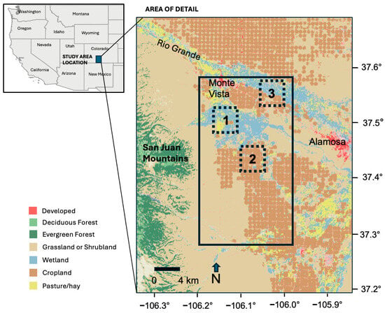
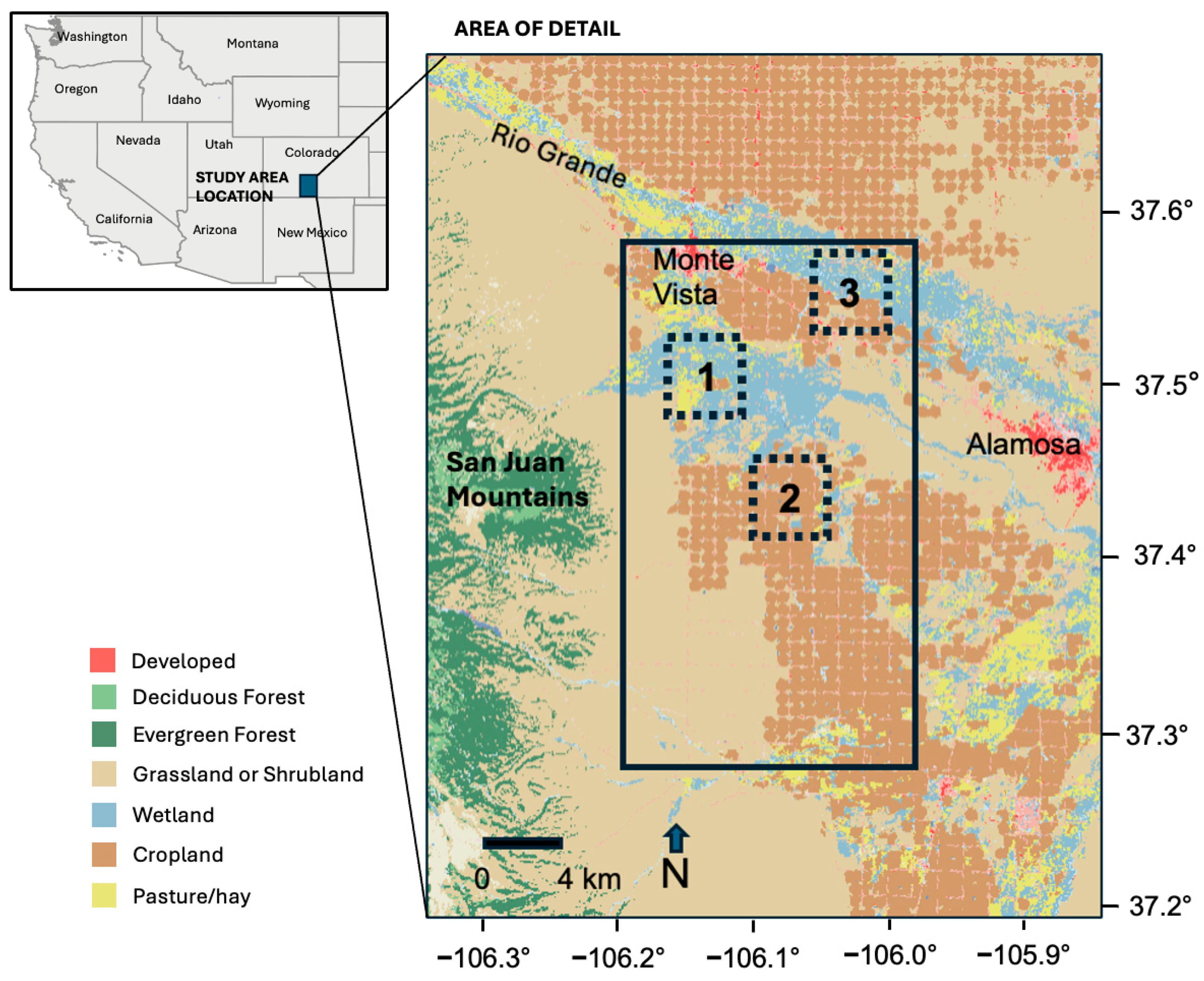
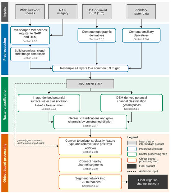
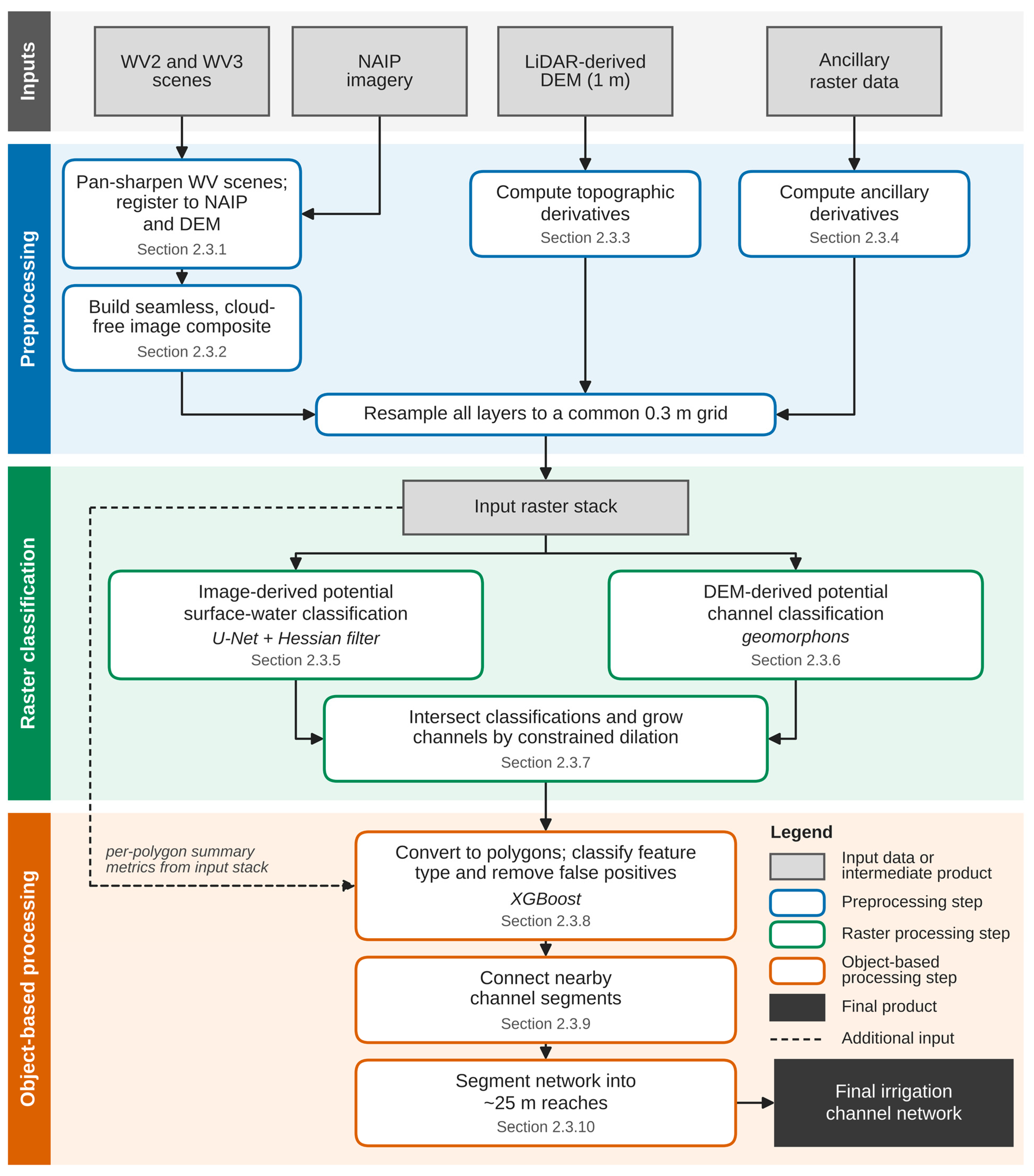
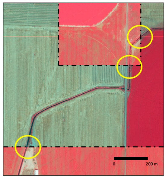
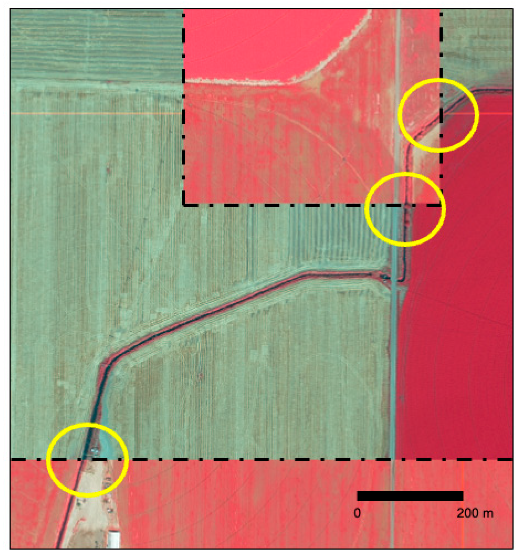
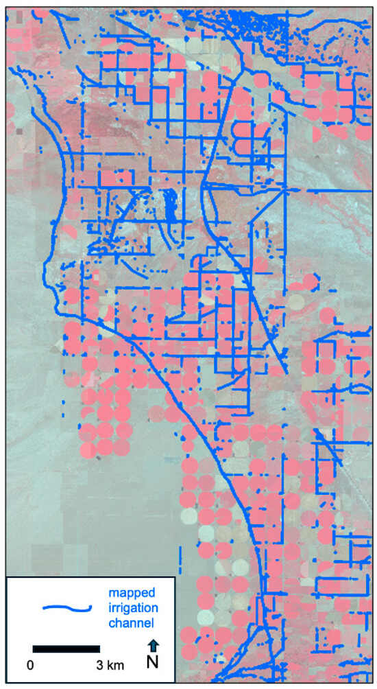
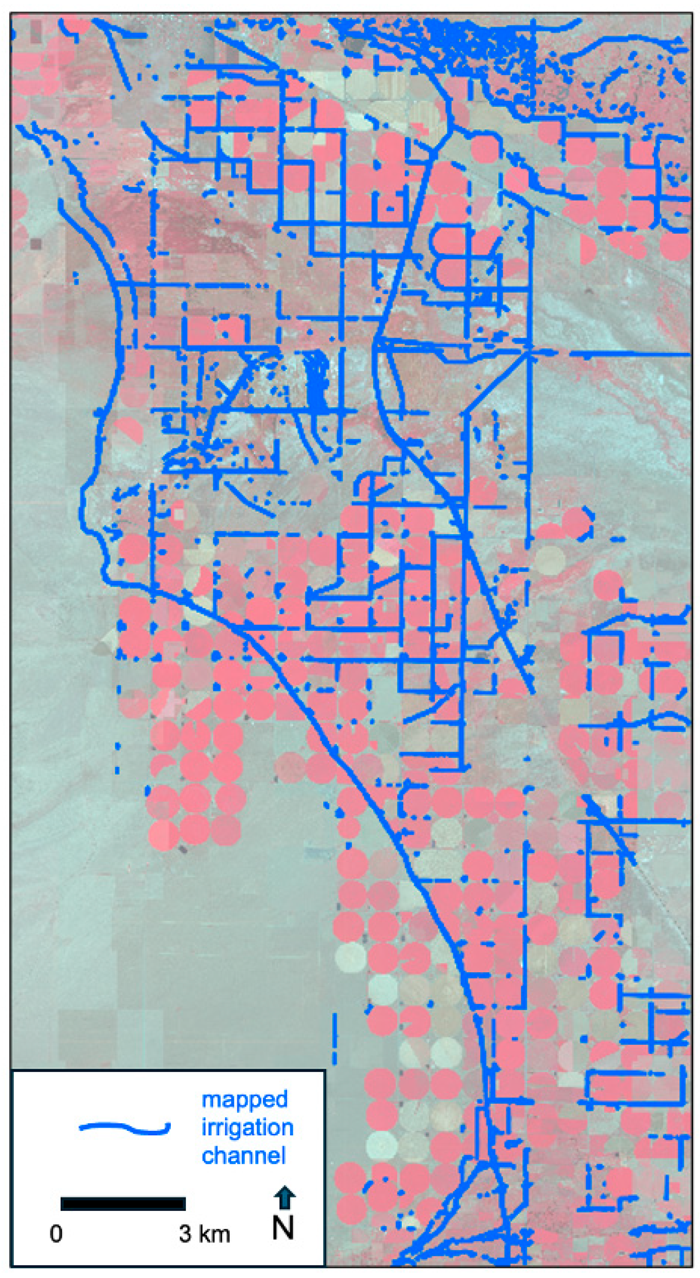
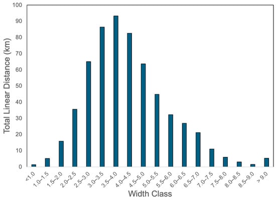
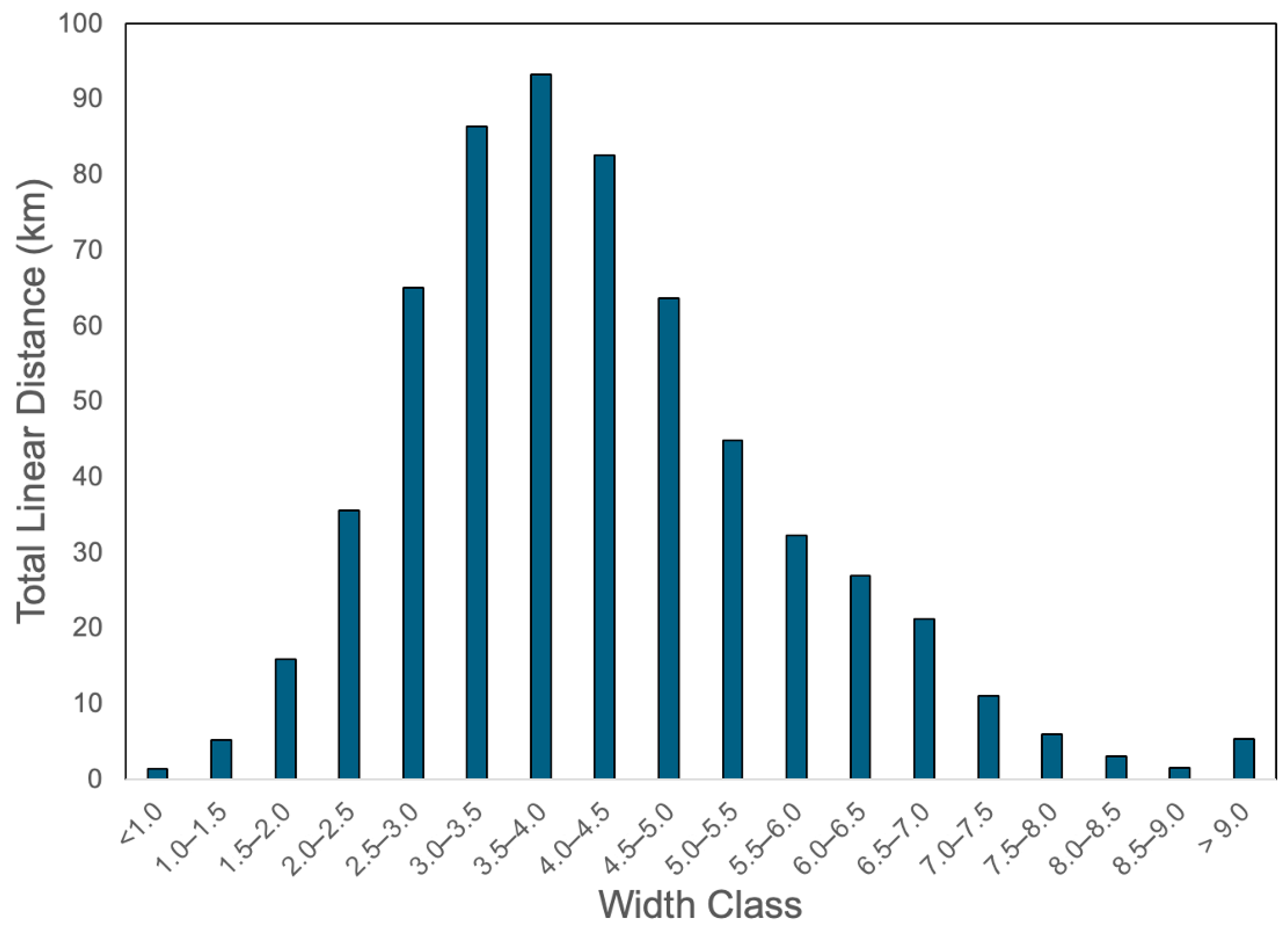
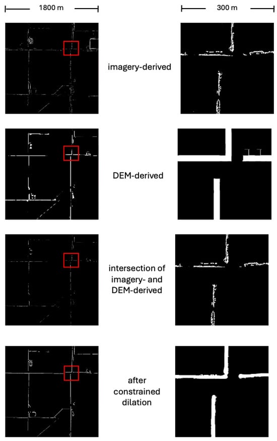
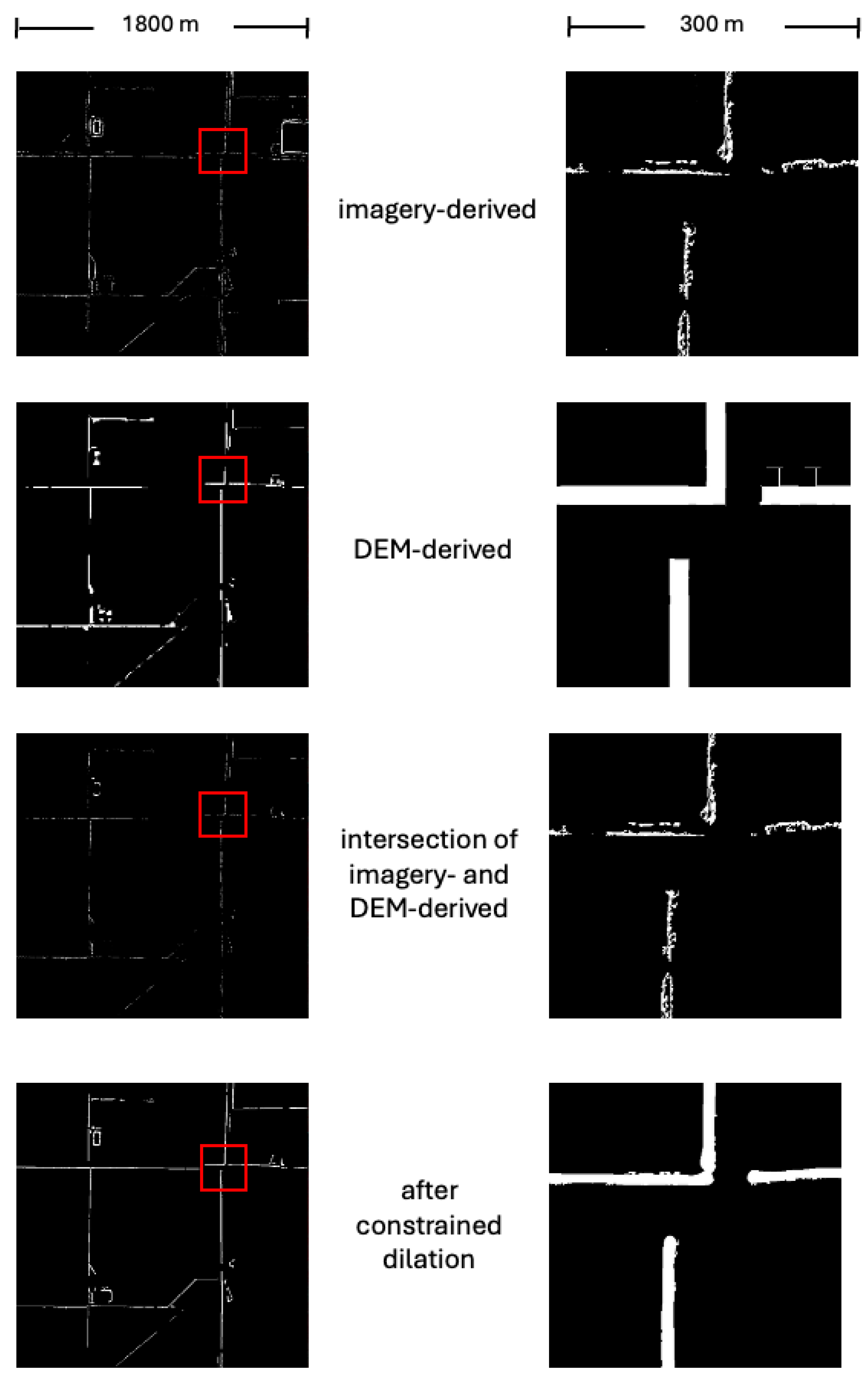
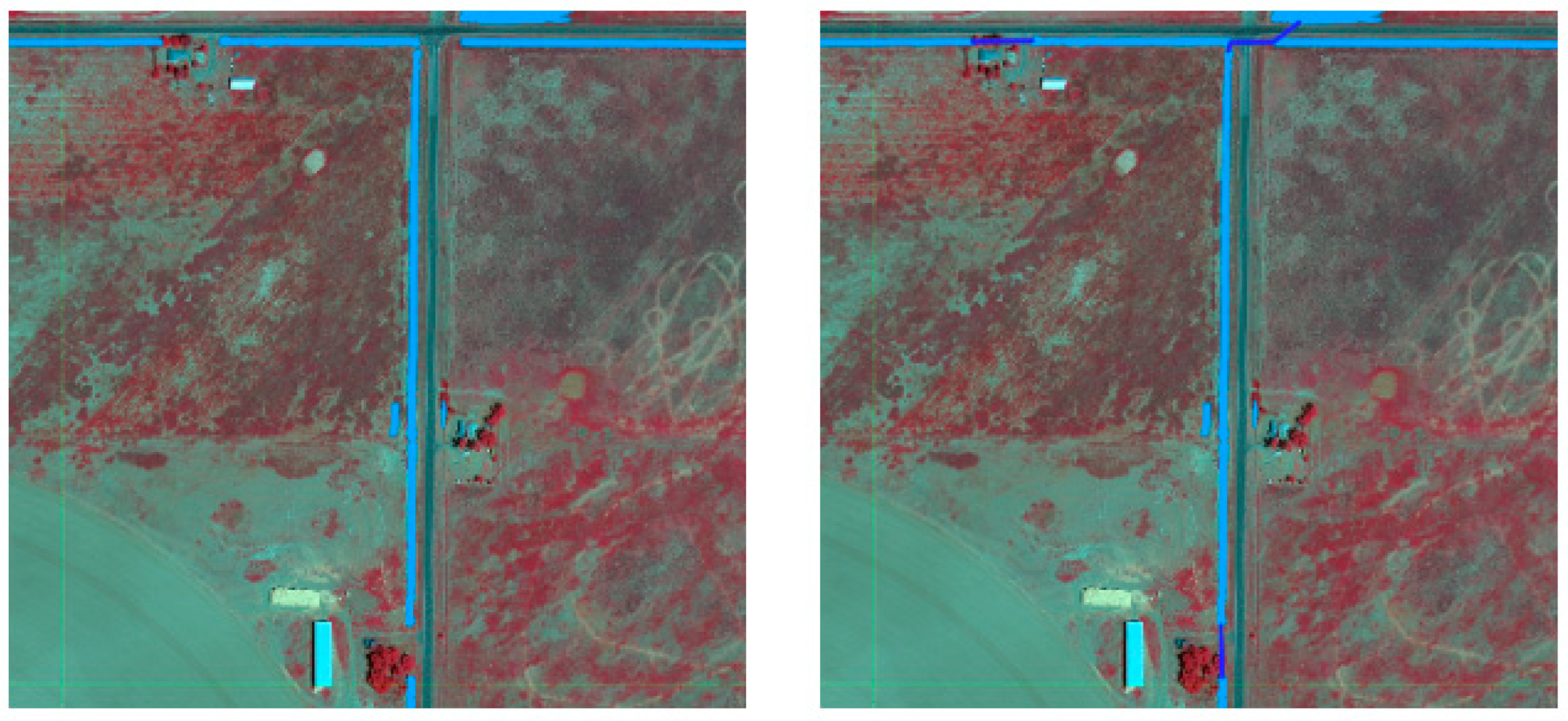
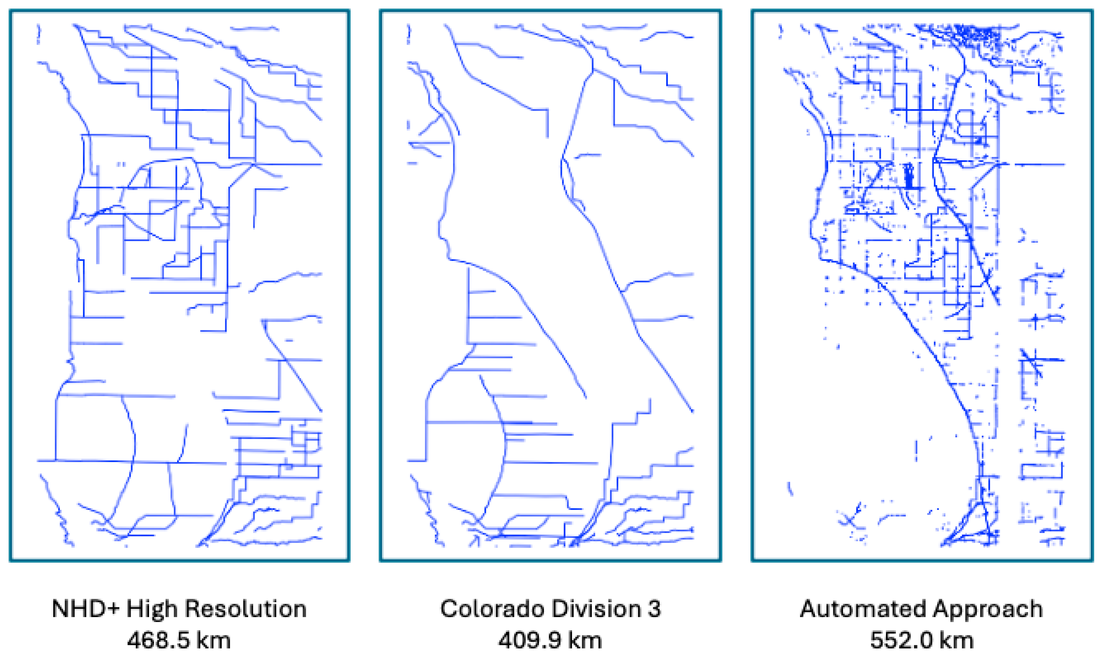
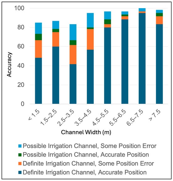
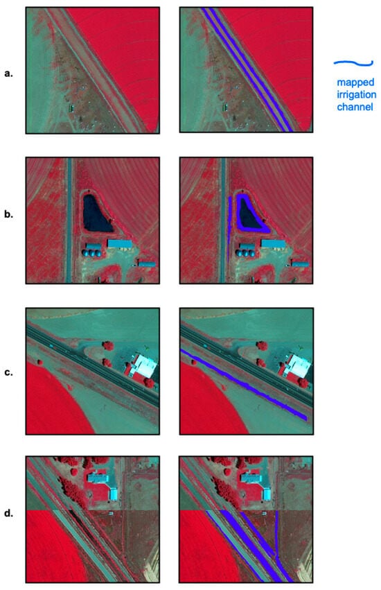
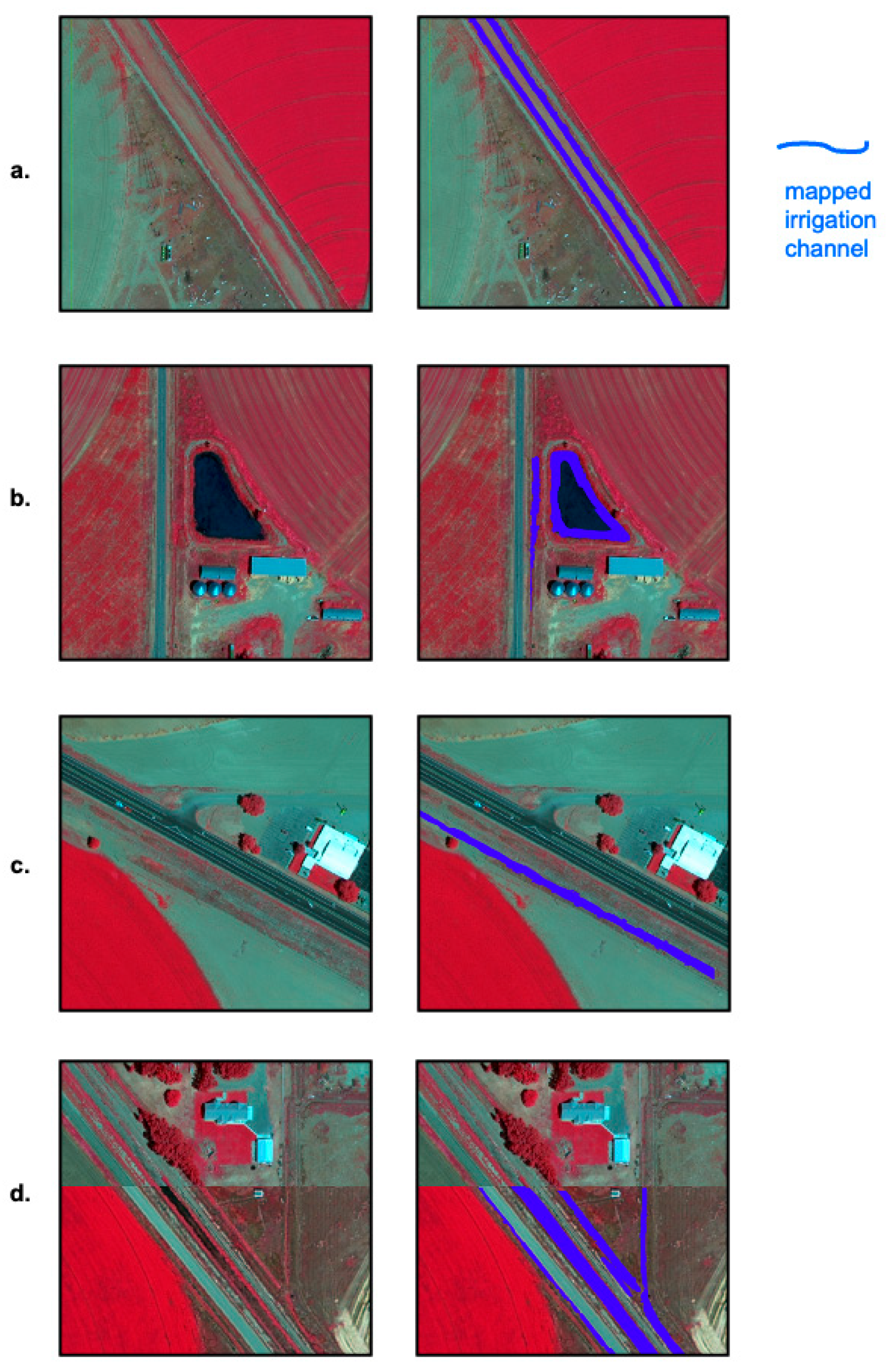

Disclaimer/Publisher’s Note: The statements, opinions and data contained in all publications are solely those of the individual author(s) and contributor(s) and not of MDPI and/or the editor(s). MDPI and/or the editor(s) disclaim responsibility for any injury to people or property resulting from any ideas, methods, instructions or products referred to in the content. |
© 2026 by the authors. Licensee MDPI, Basel, Switzerland. This article is an open access article distributed under the terms and conditions of the Creative Commons Attribution (CC BY) license.