


Highlights
What are the main findings?
- A multi-track L-band/C-band DS-InSAR survey of the Daguan county seat resolves coherent points per from LT-1 against from Sentinel-1, a 23.74-fold gain that is largest in vegetated terrain.
- Two-dimensional decomposition and SSA show that the resolved motion at H01–H03 is dominated by east–west displacement, that the 2026 rebound at H03 is reproduced by the seasonal component rather than by a reversal of the trend, and that east–west seasonal deformation is associated with maximum air temperature (r = 0.364–0.466) rather than with rainfall at zero lag.
What are the implications of the main findings?
- By characterizing the deformation and its candidate driving mechanisms at the Daguan county seat, this study provides a concrete basis—three delineated deforming sites with their rates, time-series behavior and relative monitoring priority—for geological hazard identification and for disaster prevention and mitigation in the county.
- Separating trend from seasonal amplitude changes the operational reading of a raw displacement curve (at H03 it avoids misreading a seasonal rebound as stabilization), and it frames thermal cycling, seismic shaking and slope cutting as candidate drivers whose mechanistic attribution still requires field, geotechnical and construction records.
Abstract
Daguan County, in the Wumeng Mountains of Yunnan Province, Southwest China, is characterized by complex tectonics, steep terrain and highly seasonal rainfall, and is among the counties most severely affected by geological hazards in the province. This study applies distributed-scatterer time-series InSAR (DS-InSAR) to ascending and descending SAR imagery acquired between March 2024 and July 2026 by the L-band LuTan-1 (LT-1) constellation and by C-band Sentinel-1, deriving wide-area line-of-sight (LOS) velocity fields and deformation time series over a monitoring area of about around the county seat. Ascending–descending decomposition and singular spectrum analysis (SSA) separate the deformation at three deforming sites into trend, periodic and residual components, and cross-correlation, lag-response, cumulative regression and wavelet coherence analyses are used to test the temporal association between deformation and meteorological and other external variables. LT-1 shows a clear advantage in vegetated terrain: the ascending stack yields coherent points per , a 23.74-fold density (2274.0% increase) relative to Sentinel-1 and a 42.22-fold density (4122.3%) within vegetated areas, while the descending stack yields points per (10.55-fold, 954.6%; 22.87-fold, 2186.9% in vegetated areas). Because the two stacks also differ in incidence and azimuth angle, acquisition dates, repeat cycle and processing thresholds, this gain is reported as an operational advantage of the L-band mission rather than as an isolated wavelength effect. At significant-deformation points the two missions agree with correlation coefficients of 0.674 and 0.623 and root-mean-square errors of 15.32 and 2.72 mm/yr; this is moderate agreement, and the ascending comparison rests on only 49 matched pairs. Three clusters of significant deformation (H01–H03) were delineated for mm/yr. Two-dimensional decomposition indicates that the resolved motion is dominated by east–west horizontal displacement (mean rates of , and mm/yr, peak of mm/yr at H03), with horizontal-to-vertical trend ratios of 5.30, 1.79 and 4.16; because the north–south component is not resolved, these ratios describe an apparent horizontal dominance whose magnitude depends on the decomposition assumption. SSA reveals cumulative east–west trend displacements of mm at H01, mm at H02 and mm at H03, where the trend rate increases to mm/yr. At H03 the periodic amplitude of 30.46 mm reproduces most of the apparent rebound present in the raw series, so the rebound should not be read as stabilization; under the adopted decomposition it does not require a reversal of the trend. The east–west periodic component is associated with maximum air temperature (r = 0.364, 0.439 and 0.466) but only weakly with rainfall at zero lag. Following the M 3.9 earthquake of 12 December 2025, trend rates at H01 and H03 increased briefly, and the acceleration at H01 and H02 coincides in time with the period of most intensive urban construction; these coincidences are consistent with, but do not demonstrate, seismic and engineering triggering.
1. Introduction
The mountainous regions of Southwest China lie along the complex tectonic belt of the eastern Tibetan Plateau, where steep relief, fractured rock masses and abundant rainfall make geological hazards frequent and widespread [1,2]. Daguan County, in the hinterland of the Wumeng Mountains in Yunnan Province, is among the counties most severely affected by geological hazards in the province [3]. The development and distribution of landslides there are jointly controlled by topography, stratigraphy and rainfall, and the county has long carried a high level of geological hazard risk [3]. A particularly notable situation is that the county seat, Cuihua Town, is built entirely on the accumulation body of the Daguan giant ancient landslide. Under the influence of rainfall, earthquakes and slope cutting for urban construction, creep deformation is now occurring at several locations on the body, which hosts 40 secondary landslides on its surface and in its immediate surroundings, some of which show signs of localized reactivation [4,5]. Reactivation of ancient landslides is one of the principal threats to urban development in the mountainous regions of Southwest China [6,7]. The failure mechanisms of high-position landslides and of large rock landslides in strongly seismic regions have been studied in depth [8], and the reactivation and deformation of ancient landslides in reservoir areas and river valleys have been widely reported [9]. In recent years, typical hazards such as the Shangba Village landslide near Tianxing Town and the Qinggang Village landslide along the Neijiang–Kunming railway [3] have occurred or continued to deform, posing a direct threat to mountain towns and to lifeline infrastructure.
Interferometric Synthetic Aperture Radar (InSAR), which can acquire surface deformation with all-weather, day-and-night, wide-area coverage at millimetre-level precision, has become a core technology for the identification and dynamic monitoring of geological hazards [10,11]. Since the introduction of Persistent Scatterer InSAR (PS-InSAR) and the Small Baseline Subset (SBAS) approach [12,13,14], time-series InSAR methods have developed continuously. The StaMPS approach achieves robust time-series solutions for point targets without an a priori scattering model [15,16]. SqueeSAR incorporates distributed scatterers (DS) into a unified inversion framework and thereby substantially increases the density of measurement points over low-coherence surfaces such as vegetated and bare-soil areas [17]. On this basis, statistical homogeneous pixel selection [18] and efficient phase estimation based on eigenvalue decomposition of the covariance matrix (EMI) have further improved the robustness and efficiency of DS phase optimization [19,20,21,22,23]. Alongside these methodological advances, self-referenced accuracy assessment of time-series InSAR products has become feasible through the three-cornered hat approach, which jointly analyzes deformation time series obtained from three or more independent techniques to estimate the individual error of each without external reference data [24]. These methods have been applied extensively to wide-area identification of landslide hazards, monitoring of ancient landslide reactivation and monitoring of reservoir-bank and urban deformation along the eastern margin of the Tibetan Plateau, in the Jinsha River basin and in the mountainous areas of Sichuan and Yunnan [6,25,26,27]. Of particular interest is the LuTan-1 (LT-1) L-band SAR satellite, whose wavelength of approximately 23.7 cm gives it strong penetration through vegetation. It has already demonstrated a distinctive advantage in monitoring large landslide displacements and in the early identification of geological hazards, and it provides a new data source for deformation monitoring in the densely vegetated and steep terrain of Southwest China. Regional landslide hazard assessment has evolved from qualitative identification through statistical models to physically based models [8,28,29], and the deformation and failure mechanisms of high slopes continue to be investigated [6]. Machine learning methods have also been widely applied to landslide susceptibility assessment.
As far as Daguan County is concerned, previous studies fall broadly into two categories. The first comprises regional susceptibility and hazard assessments based on static factors, such as susceptibility mapping based on frequency ratio and index-of-entropy models [30] and analyses of slope and aspect sensitivity [3]. The second comprises engineering-geological analysis and stability assessment of individual landslides, including numerical simulation of the deformation characteristics and reactivation mechanism of the Daguan ancient landslide [4], study of the reactivation mechanism of an ancient landslide under the combined action of rainfall and upper loading [31], analysis of the causes of the Shangba Village landslide [3], and analysis of the relationship between the evolution of ancient landslide bodies and urban spatial expansion [5].
Taken together, the existing research suffers from two shortcomings. First, in terms of spatial scale, regional susceptibility assessment relies on static topographic and geological factors and on historical hazard inventories. It answers the question of where hazards are likely to occur, but not where deformation is currently taking place, at what rate, or whether it is accelerating or decelerating. Single-site engineering-geological analysis, by contrast, cannot cover the scale of an entire county, leaving conspicuous blind spots in densely vegetated and inaccessible areas, and it struggles to capture the slow reactivation of ancient landslides. Second, in terms of temporal dimension, the long-term creep trend, seasonal periodic fluctuation and short-term random disturbance contained in a deformation time series correspond respectively to progressive strength decay, seasonal modulation by climatic factors such as rainfall and temperature, and the effects of sudden events such as earthquakes and human engineering activity. Each is therefore of interest for interpretation and warning, although the mapping from a statistical component to a physical process is not unique (Section 4.3). Yet no study of Daguan County has systematically decomposed the deformation time series of the county seat and its immediate surroundings—a monitoring area of about (Section 2.1) rather than the whole county—and quantified the association and lag characteristics between deformation and multiple candidate drivers.
Three points define the contribution of this study relative to the work summarized above. The central one is the hazard analysis itself: this study uses multi-track L-band and C-band time-series InSAR to characterize the deformation of the county seat of Daguan and of the ancient landslide body on which it is built, to separate the observed motion into trend, seasonal and residual components, and to examine, under an explicit statistical protocol, how each component is associated with rainfall, temperature, the December 2025 earthquake and engineering activity, thereby identifying a set of candidate deformation drivers and providing a concrete basis—the delineation of three deforming sites, their rates, their time-series behavior and their relative monitoring priority—for hazard identification, dynamic monitoring and disaster prevention and mitigation in this county. The methodological contribution is secondary but not negligible: the individual techniques are established ones and we do not claim them as new, yet their combination in a dual-geometry design that pairs an L-band constellation with a C-band mission delivers a coherent-point density in vegetated terrain tens of times higher than what a C-band survey alone provides, and it is this density that makes the deformation field of an urban area built on an ancient landslide body resolvable in the first place. To our knowledge this is the first study of Daguan County that separates the observed deformation into trend, seasonal and residual components and then reports the association of each component with meteorological, seismic and anthropogenic variables under a stated statistical protocol, and we make the evidential status of each statement explicit throughout: the InSAR results are treated as observations, the correlation, lag and wavelet analyses as tests of temporal association, and the mechanistic reading as a set of candidate drivers with stated conditions of validity. A practical point follows from the separation itself: the trend and seasonal components carry different operational information, so that a raw displacement curve alone can be misread at a site such as H03, where the two oppose one another. The study does not, and cannot, establish physical mechanisms: it has no geodetic validation, no geotechnical profiling and no construction records, and the corresponding statements are framed accordingly throughout.
In view of this, the present study takes the county seat of Daguan County and the surrounding ancient landslide bodies as the study area and uses ascending and descending SAR imagery acquired since March 2024 by Sentinel-1 (C-band) and LT-1 (L-band) to address the following objectives: (1) to derive LOS deformation velocity fields and deformation time series using distributed-scatterer time-series InSAR (DS-InSAR) and, by exploiting the complementarity of the two missions and of ascending and descending geometries, to achieve wide-area identification and inventorying of geological hazards; (2) to separate the LOS deformation into vertical and east–west components by ascending–descending decomposition, and to characterize the spatial motion and principal deformation direction of typical landslides; (3) to decompose the deformation time series of typical deforming areas into trend, periodic and residual components using singular spectrum analysis (SSA) and wavelet analysis, and to identify deformation signals at different scales, namely long-term creep, seasonal fluctuation and sudden disturbance; and (4) to test the temporal association and lag characteristics between the deformation of the typical deforming sites and rainfall, temperature, seismic and engineering-activity data using cross-correlation, lag-response and wavelet coherence analyses, treating the outcome as candidate drivers rather than as demonstrated mechanisms. The results are intended to provide a scientific basis for the identification, dynamic monitoring and mitigation of geological hazards in the Wumeng Mountains and, more broadly, in the mountainous regions of Southwest China.
2. Materials and Methods
2.1. Study Area
Daguan County lies in the northeastern part of Yunnan Province, in the hinterland of the Wumeng Mountains. The terrain is generally high in the north and south and low in the middle. Elevation ranges from a maximum of 2758 m in the south of the county to a minimum of 492 m in the north, a relative relief of 2293 m, with a mean elevation of about 1600 m. Slopes steeper than cover about , or 54% of the total area [3]. The geomorphology is dominated by tectonically dissected mid- and high-mountain gorges and can be divided into two categories, namely tectonically denuded and karstified mountain terrain and deeply incised river valley terrain [3]. The county has a northern subtropical plateau monsoon climate with pronounced vertical zonation. The mean annual temperature is 15 °C, with an extreme maximum of 40.3 °C and an extreme minimum of −6.4 °C. Mean annual precipitation is about 970–1120 mm, concentrated between June and September, which accounts for roughly 80% of the annual total, and the mean daily torrential rainfall is 70–120 mm [3]. All rivers within the county belong to the Jinsha River system, and the valleys are deeply incised with steep slopes and deep gorges.
Tectonically, Daguan County lies at the margin of the Upper Yangtze ancient landmass (the Yangtze paraplatform) and in the northern segment of the Sichuan–Yunnan meridional tectonic belt, within the middle section of the Ludian–Yanjin tectonic belt. Folds and faults are well developed in the area, trending generally northeast, and the spacing of faults is distinctly regular [3]. Strata exposed in the county range from the Paleozoic Cambrian to the Mesozoic Triassic, and consist mainly of shallow-marine carbonate rocks and littoral to paralic clastic rocks. The only igneous rock is the Upper Permian Emeishan basalt. Quaternary loose deposits are widely distributed in gullies and on slopes. In terms of engineering-geological characteristics, the rock masses can be divided into weak clastic rocks, carbonate rocks with intercalated clastic rocks, dolomite and limestone, massive dolomite and limestone, and basalt engineering-geological groups [3]. With respect to the seismic environment, the study area lies close to highly active seismic belts including the Wulianfeng fault zone and the Zhaotong–Ludian fault zone. Since 1900, 104 earthquakes of surface-wave magnitude have occurred in the region, including seven of magnitude 6.0–6.9 and two of magnitude 7.0–7.9. The peak ground acceleration is 0.15–, corresponding to seismic intensities of VII–VIII [4].
Against this geological and environmental background, geological hazards in Daguan County are numerous, widely distributed and frequent, and the county is among the most severely affected in Yunnan Province [3]. The county has long been subject to a high level of geological hazard risk [3]. Debris-flow gullies within the county are concentrated in Gaoqiao and Yuele towns, and are best developed in the Gaoqiao River basin. Existing landslides are dominated by push-type (43.5%) and retrogressive (31.1%) failures, and small landslides account for 88.3% of the total [3]. The county seat, Cuihua Town, is situated on the accumulation body of the Daguan giant ancient landslide, which can be divided morphologically into three levels of gentle slope [4]. Between 1970 and 2022 the urban area of Daguan County expanded approximately 7.56-fold. As a result of this urban expansion, five new landslides and six reactivated secondary landslides on the surface of the ancient landslide body are concentrated near the residential expansion zones and road-excavation areas, and slope cutting for house construction and excavation for road building have become the main anthropogenic factors affecting slope stability [5]. Human activity is concentrated in the deeply incised valleys and the piedmont accumulation zones, where inappropriate site selection for buildings and slope cutting and engineering fill at the toe of slopes have aggravated slope deformation.
The study area for the deformation analysis presented here covers the county seat and the surrounding ancient landslide body, between 103. and 103.E and between 27. and 27.N (Figure 1). It is bounded by the common footprint of the four stacks and covers about ; this monitored area, and not the of the county as a whole, is the spatial unit to which all densities and proportions reported below refer.
Figure 1.
Location and setting of the study area. (left) Regional setting of Daguan County showing the county boundary, the main rivers and towns, and the coverage of the Sentinel-1 and LT-1 SAR scenes. The red rectangle marks the deformation-monitoring study area. (right) High-resolution optical image of the county seat, with the boundary of the Daguan giant ancient landslide body outlined in red.
2.2. Data
2.2.1. SAR Data
This study uses ascending and descending SAR imagery acquired by Sentinel-1 and by the LuTan-1 (LT-1) constellation between March 2024 and July 2026 for time-series deformation monitoring. Sentinel-1 is a C-band (wavelength approximately 5.6 cm) SAR mission of the European Space Agency’s Copernicus program. It operates in Interferometric Wide Swath (IW) mode with a swath of 250 km, nominal range and azimuth resolutions of about 5 m and 20 m respectively, and a single-satellite repeat cycle of 12 days (6 days when two satellites operate in constellation) [32]. LT-1 is China’s first L-band differential interferometric SAR satellite constellation and consists of the two satellites LT-1A and LT-1B. It was launched in 2022 and entered formal operational service in December 2023. It orbits at an altitude of about 607 km and operates at L-band (wavelength approximately 23.7 cm), with nominal resolutions of 3–12 m and swaths of 50–100 km in Stripmap mode, a single-satellite repeat cycle of 8 days and a constellation repeat cycle of 4 days, and a design lifetime of 8 years. The parameters of the two datasets are compared in Table 1.
Table 1.
Comparison of Sentinel-1 and LT-1 SAR data parameters.
Compared with C-band Sentinel-1, the L-band signal of LT-1 has a wavelength about 4.2 times longer, which gives it stronger penetration through the vegetation canopy and surface roughness and better temporal coherence. It therefore yields denser and more stable coherent measurement points over densely vegetated and rapidly decorrelating surfaces, which makes it well suited to a county such as Daguan with high vegetation cover and steep terrain.
The comparison between the two missions is not a controlled experiment, and we report it accordingly. The two stacks differ in wavelength, incidence and azimuth angle, acquisition dates, repeat cycle, spatial resolution, number of scenes and processing thresholds, so that an identical physical displacement field would still project differently onto the two lines of sight, and the size of the coherent point set depends on coherence, on the SHP selection settings and on the number of usable interferometric pairs. The same SHP settings, the same significance threshold and the same reference area were used for both missions, which removes the processing difference as far as the available data allow, but it cannot remove the geometric and temporal differences. We therefore report the density difference as an operational advantage of the L-band mission for hazard screening in vegetated terrain, quantify it in both percentage and fold terms, and do not attribute it to wavelength alone; the controlled, single-parameter comparison that would be required to isolate the wavelength effect is not possible with these two missions.
2.2.2. Auxiliary Data
The auxiliary data used in this study comprise four categories: DEM data, precise orbit data, meteorological data and an earthquake catalogue. The DEM is the TanDEM-X 30 m Edited Digital Elevation Model (EDEM) with a spatial resolution of 30 m (corresponding to a pixel spacing of 1 arc-second at the equator). The data were acquired during the TanDEM-X mission between 2010 and 2014 and were developed and released by the Microwaves and Radar Institute of the German Aerospace Center (DLR). For precise orbits, Sentinel-1 uses the POD precise orbit ephemeris products (including RESORB and POEORB) generated by the Copernicus POD Service of the European Space Agency (ESA), which are mirrored and distributed by the Alaska Satellite Facility (ASF) on the AWS cloud platform. LT-1 uses the precise orbit products of the China Centre for Resources Satellite Data and Application, which is responsible for the construction, operation and management, data processing, calibration, archiving, distribution and servicing of the ground processing system. The meteorological data consist of daily precipitation and temperature observations from the Daguan County meteorological station, obtained from the Meteorological Data Centre of the China Meteorological Administration. The earthquake catalogue is the national seismic network catalogue published by the China Earthquake Networks Centre and is available from the National Earthquake Science Data Centre. Table 2 summarises the auxiliary data.
Table 2.
Auxiliary data used in this study.
2.3. Overall Technical Framework
The technical framework of this study follows the chain “multi-source SAR data synergy–DS-InSAR time-series inversion–construction of the deformation field and hazard identification–decomposition of deformation signals–analysis of candidate drivers”, as illustrated in Figure 2. The framework comprises five levels, namely the data level, the preprocessing level, the DS-InSAR processing level, the deformation-result and hazard-identification level, and the signal-decomposition and driving-mechanism level. Data and processing flow pass progressively from one level to the next.
Figure 2.
Technical workflow of the study, from multi-source SAR data and preprocessing through DS-InSAR time-series inversion, hazard identification, signal decomposition and driving-mechanism analysis.
At the data level, ascending and descending SAR imagery from Sentinel-1 and LT-1 acquired between 2024 and 2026 is collected. Sentinel-1 provides wide-swath C-band observations and LT-1 provides L-band data with strong vegetation penetration. In parallel, a TanDEM-X 30 m DEM, precise orbit (POD) data for both missions, and meteorological and earthquake data are obtained, providing multi-source input for the subsequent time-series InSAR processing and driving-mechanism analysis.
At the preprocessing level, master–slave registration and differential interferometric processing are carried out separately for the Sentinel-1 and LT-1 ascending and descending imagery to generate intensity images and differential interferograms. Flat-earth and topographic phases are removed so as to provide the basic interferometric data for PS/DS point identification and time-series inversion.
At the DS-InSAR processing level, PS and DS points are jointly identified from the differential interferograms. For DS candidates, the Kolmogorov–Smirnov (KS) test is used to select statistically homogeneous points (SHPs), and the sample coherence matrix of the homogeneous samples is estimated. Phase optimization and filtering are then performed using the eigenvalue-decomposition-based maximum-likelihood phase linking (EMI) algorithm, which improves phase quality in vegetated areas. Finally, the PS points and the optimized DS points are brought together into the StaMPS time-series inversion framework to complete three-dimensional phase unwrapping, atmospheric correction and removal of orbital errors and topographic residuals, yielding time-series deformation rates and cumulative deformation.
At the deformation-result and hazard-identification level, ascending and descending LOS deformation fields of the study area are obtained, and a comparison between LT-1 and Sentinel-1 in the LOS direction is carried out to evaluate the monitoring advantage of the L-band data in vegetated mountainous terrain in terms of coherent-point density, consistency of deformation rates and root-mean-square error. Ascending and descending observations are then used for two-dimensional decomposition to solve for the vertical and east–west deformation components and to determine the principal direction of landslide motion. On this basis, and combining rate thresholds, time-series shape, spatial continuity, ancient landslide boundaries and the existing hazard inventory, geological hazards are identified and inventoried, and the typical hazard sites H01–H03 are delineated.
At the signal-decomposition and driving-mechanism level, deformation time series are extracted for the typical hazard sites or deforming areas and analyzed. Singular spectrum analysis (SSA) is used to decompose each time series into trend, periodic and residual components. The trend component characterizes long-term creep and episodic acceleration or deceleration. The periodic component is used to analyze the seasonal response of deformation to meteorological factors such as rainfall and temperature. The residual component is used to identify sudden disturbances such as earthquakes and human engineering activity. Pearson correlation, cross-lag correlation, cumulative regression and wavelet coherence analysis are then used to quantify the relationships and lag characteristics between deformation and multiple factors including rainfall, temperature, earthquakes and human engineering activity. Finally, based on the deformation characteristics and driving-mechanism analysis, target areas for monitoring and early warning are proposed together with disaster-prevention recommendations.
Through this framework the study establishes a complete analytical chain that runs from wide-area deformation monitoring to hazard identification, from decomposition of deformation signals to analysis of candidate drivers, and from deformation analysis to disaster-prevention application, providing a new technical approach for the identification, dynamic monitoring and mitigation of geological hazards in the Wumeng Mountains and in the mountainous regions of Southwest China.
2.4. DS-InSAR Time-Series Deformation Monitoring
2.4.1. Interferometric Phase Model
For two SAR images covering the same area and acquired at different times, after registration and interferometric processing and after removal of the flat-earth and topographic phases, the interferometric phase can be written as [33]
where the terms denote, respectively, the deformation phase along the line of sight (LOS), the residual topographic phase (proportional to the elevation error ), the long-wavelength phase caused by residual orbital error, the atmospheric delay phase, and thermal noise and spatiotemporal decorrelation noise. It should be noted that interferometry is significantly affected by temporal, spatial and volumetric decorrelation [34,35,36]. This is precisely why PS/DS joint inversion methods must be developed in the time domain.
After phase unwrapping and error correction, the relationship between the LOS deformation and the deformation phase is
where is the radar wavelength. The negative sign indicates that deformation moving away from the satellite (subsidence, or motion towards the east) corresponds to a negative phase change.
2.4.2. Identification of Distributed Scatterers and Phase Optimisation
In vegetated areas, the scattered echo within a single pixel is often composed of a large number of small scatterers whose scattering properties remain relatively stable over time. Such pixels are distributed scatterers (DS). Unlike PS targets, DS require the phase to be estimated jointly over time using statistical methods. The DS processing chain adopted here is as follows. First, with the target pixel at the centre, the Kolmogorov–Smirnov (KS) test is applied within a defined window at a given confidence level to determine whether the amplitude samples of neighbouring pixels are statistically homogeneous with those of the central pixel, and the set of statistically homogeneous points (SHPs) is selected [17,18,22,23,37]. The temporal sample coherence matrix is then estimated from the SHP samples, and the eigenvalue-decomposition-based efficient phase estimation (EMI) algorithm is used to estimate the optimal phase sequence of each pixel in the least-squares sense [19,20,21]. Specifically, if the time-series complex observation vector of a DS pixel is , its sample coherence matrix can be expressed as
where M is the number of SHPs and the superscript H denotes the conjugate transpose. The EMI method transforms the estimation of the optimal phase vector into an eigenvalue decomposition of the coherence matrix:
where denotes the element-wise modulus of the sample coherence matrix, ∘ represents the Hadamard (element-wise) product, and is the normalized coherence matrix. The eigenvalues and the corresponding eigenvectors of are obtained from the decomposition. Under the least-squares criterion, the optimal phase sequence is given by the principal eigenvector corresponding to the largest eigenvalue of :
where is the principal eigenvector corresponding to the largest eigenvalue of . This method improves computational efficiency substantially while preserving accuracy and robustness [19].
The implementation settings are as follows. The KS test was applied in a 15 × 15 pixel window at a confidence level of 0.95 with a minimum of 20 SHPs per pixel; the amplitude samples were normalized before the test. The final multilooked pixel spacing was about 10 m for LT-1 and about 20 m for Sentinel-1, and the number of looks therefore differs between the two missions, which is one reason why their point densities are not strictly comparable (Section 4.1). EMI phase linking was iterated to convergence with a boxcar filter applied to the linked phase, and phase unwrapping was performed with the minimum-cost-flow method using SNAPHU v2.0.6 within the StaMPS v4.1b framework running on MATLAB (The MathWorks, Inc., Natick, MA, USA). All four stacks were referred to the same stable reference point at 103.E, 27.N, selected outside the mapped deforming ground on bedrock with high coherence in all four geometries.
2.4.3. Time-Series Inversion
PS candidate points and the phase-optimized DS points are taken together as the points to be solved, and time-series inversion is performed using the point-target framework of StaMPS [15,16]. Its core idea is to separate the deformation phase, residual topographic phase, atmospheric phase and noise point by point through statistical analysis of the phase of each interferogram in the temporal and spatial dimensions. The procedure comprises interferometric phase unwrapping, separation of atmosphere and orbital error by spatial high-pass and temporal low-pass filtering, estimation and correction of elevation error, and finally atmospheric phase filtering and geocoding [16,38]. After these steps, the mean LOS deformation rate and the deformation time series for each coherent point are obtained.
2.5. Two-Dimensional Decomposition of LOS Deformation
The LOS deformation from a single orbit is a one-dimensional projection of three-dimensional surface deformation onto the line of sight, whose direction is determined by the incidence angle and the satellite flight azimuth . For the i-th observation (or for the ascending/descending orbit), the relationship between the LOS deformation rate of a given observation and the eastward, northward and vertical deformation rates is
Because InSAR is very insensitive to north–south deformation, the northward term is normally neglected. For a single orbit the observation equation reduces to
and ascending and descending observations are combined to solve for and :
The nominal incidence and azimuth angles used for the two geometries are given in Table 3: 39. (ascending), 26. (descending), 259. (ascending azimuth) and 101. (descending azimuth), the scene-center values read from the LT-1 attitude files. These are the scene-center values; local terrain-related incidence angles were not used, so that in steep terrain the projection coefficients are approximate, with an error that grows with local slope. The ascending and descending stacks were referred to the same reference area (a stable point at 103.E, 27.N, outside the mapped deforming ground) before decomposition, and the two time series were compared at the acquisition dates common to both, with linear interpolation in between; the interpolation error is small compared with the rate differences discussed below but is not zero.
Table 3.
Geometric parameters used for the two-dimensional decomposition (scene-center nominal values).
Three limitations of the decomposition equation must be stated explicitly. First, is set to zero, which is justified only when the north–south component is small compared with the other two. For the sites studied here this cannot be assumed a priori, because the slopes face in various directions. The neglected term contributes to the modeled LOS rate, so that the retrieved east–west and vertical components absorb part of ; the size of this effect is bounded by and by the conditioning of , and it is largest where the two lines of sight are close to parallel, that is, where the difference in incidence angle between the ascending and descending geometries is small. Second, a single nominal angle per track replaces the local geometry. Third, the decomposition assumes that the surface moves as a rigid block at the scale of a pixel, which is adequate for a first-order description but not for a differential-motion analysis. The horizontal-to-vertical ratios reported below are therefore apparent ratios; they indicate the relative importance of the two resolved components under this assumption and are not an independent measurement of the slip direction. A decomposition that resolves would require a third, independent viewing geometry or external constraint, which is not available here.
Within these limits, two-dimensional decomposition makes it possible to distinguish whether the resolved landslide deformation is dominated by horizontal or vertical motion, providing a basis for a first-order kinematic description of a landslide.
2.6. Singular Spectrum Analysis
A surface deformation time series can be regarded as consisting of three parts, namely a trend term, a periodic term and a random term. The trend term reflects long-term creep or accelerating/decelerating deformation. The periodic term reflects periodic fluctuation caused by seasonal factors such as rainfall, temperature and groundwater. The random term corresponds to observation noise and random disturbance. In this study SSA is used to decompose the deformation time series. A window length L is selected (usually between 1 and ), and the one-dimensional series is used to construct the trajectory matrix
where . Singular value decomposition is then applied to the trajectory matrix :
where the non-zero eigenvalues of the covariance matrix are ordered in descending order, the corresponding left and right singular vectors are denoted by and respectively, and d is the number of non-zero eigenvalues.
For grouping and reconstruction, the eigenvalues are grouped according to their contribution, and the first r principal components are selected to reconstruct the trend term:
The reconstructed matrix is converted back into a one-dimensional series by diagonal averaging, yielding the trend term of the series. The remaining components are further grouped by frequency to reconstruct the periodic and random terms. SSA has been widely applied to the separation of trend and periodic components of InSAR deformation time series.
The settings used in this study are as follows. A window length of L = 10 was used for the monthly sampled series (N = 29 values at roughly monthly spacing), that is, = 0.34, which is within the range recommended for separating an annual cycle from a trend of this length. The eigentriples were grouped by inspecting the scree plot of the eigenvalues, the periodogram of the elementary reconstructed components, and the w-correlation matrix; pairs of eigentriples with a common period were grouped together (the leading eigentriple for the trend, eigentriples 2–3 for the seasonal component, and the remainder for the residual), the leading group with slowly varying phase was assigned to the trend, and the residual group contained the remaining components. The variance contributions of the three groups at each site are given in the Results section (Section 3.6). The grouping follows the eigentriple indices set in the processing script (trend: index 0; seasonal: indices 1–2; residual: the remainder), and the choice of L and of the grouping is a potential source of uncertainty that is discussed in Section 4.5; a full sensitivity sweep over L and grouping has not been carried out. SSA separates a series into additive components that are orthogonal by construction; it does not assign a physical cause to any of them, and the interpretation of a component as creep, meteorological forcing or disturbance is an inference that has to be supported independently.
2.7. Correlation Analysis Between Deformation and External Factors
To quantify the relationships between deformation and factors including rainfall, temperature, earthquakes and human engineering activity, several complementary analysis methods are used here.
First, the Pearson correlation coefficient between the time series of deformation (deformation rate or periodic component) in the typical deforming areas and each meteorological factor is computed and tested for significance, in order to assess the degree of linear correlation between each factor and the deformation. For a deformation series and a factor series , the Pearson correlation coefficient r is
Second, the cross-correlation function is used to compute the correlation between the deformation series and factor series such as rainfall within a sliding window of lags from to days, and the lag corresponding to the peak correlation coefficient is taken as the response lag time of the deformation, so as to identify the seasonal acceleration pattern of rainfall-triggered landslides. The cross-correlation function is defined as
where is the lag time (), and the corresponding to the maximum of is taken as the response lag of the deformation to the factor.
Third, cross-wavelet transformation and wavelet coherence spectra [39] are used to analyze the common significant periods and phase relationships between deformation and meteorological factors at different time scales such as annual, seasonal and monthly. The cross-wavelet spectrum is defined as
and the wavelet coherence coefficient is expressed as
where the two continuous wavelet transform coefficients are those of the deformation series and of the factor series respectively, the asterisk denotes the complex conjugate, and S is a smoothing operator. The significant regions of the wavelet coherence spectrum and the direction of the phase arrows reveal the multi-scale coupling characteristics of the two series in different time–frequency domains.
Finally, the earthquake catalogue and extreme rainfall events are matched one by one against the abrupt change points in the deformation time series. By matching sudden events to abrupt change points in the deformation series, the temporal coincidence between an event and an acceleration is examined; the analysis establishes the coincidence, not the causal influence, and is reported in those terms. These methods complement one another and allow the association between deformation and natural and anthropogenic factors to be characterized from several perspectives and at several scales.
Four properties of these data constrain the statistical treatment, and we state them here because they determine how the results in Section 3.8 should be read. First, SAR acquisitions are not daily observations. The InSAR displacement series were interpolated linearly onto a daily grid so that they could be compared with the daily meteorological record, which yields 838 values between 16 March 2024 and 1 July 2026; the interpolated values are not independent observations, and the effective number of independent samples is therefore much smaller than 838. Second, deformation, rainfall and temperature are all strongly autocorrelated and seasonal, so that the classical Pearson significance test, which assumes independent samples, is anti-conservative here. We therefore report the correlation coefficients as descriptive measures of association, and interpret their significance with reference to the effective sample size estimated from the lag-1 autocorrelation of each series (lag-1 autocorrelation of the seasonal component: 0.95 at H01, 0.55 at H02 and 0.76 at H03; the effective sample size is therefore of the order of 3–9 independent values rather than the nominal 838) rather than to the nominal n = 838. Third, the lag search from 0 to 800 days tests 801 hypotheses per pair of series. With 801 tests, the probability of obtaining at least one above the 5% critical value by chance is close to unity, so a single lag peak cannot be treated as significant without correction. We report the lag of maximum for completeness, but we apply a Bonferroni-type correction to the critical value (with 801 tests, the two-tailed critical at the corrected level is about 0.49 for n = 60 and higher for smaller effective samples, so that only coefficients approaching 0.5 or above are treated as notable) and we treat peaks that fall within one seasonal cycle of the record boundary, or that are close to a multiple of the annual period, as artifacts of the search rather than as response times. Fourth, the cumulative regression of cumulative deformation on cumulative rainfall or cumulative temperature regresses two monotonically increasing series on one another, which produces high values even for independent random walks; the values in Table 8 from the cumulative-regression analysis are therefore reported as descriptive companion statistics and are not interpreted as explanatory power. The corresponding analysis on first differences, which removes the common trend, was not performed; the cumulative-regression panels in the accompanying figures are therefore retained only as a record of the analysis, not as evidence of a physical response. Finally, all statements in this paper that link a driver to a deformation signal are statements of temporal association; attribution of a physical mechanism would require independent observations (ground temperature, pore pressure, construction records, strong-motion data) that are not available for this area.
3. Results
3.1. Deformation Velocity Field of the Daguan County Seat
Using the DS-InSAR method, LOS deformation velocity fields were obtained for the study area (103.88–103.E, 27.73–27.N, covering the county seat and the ancient landslide body) from the ascending and descending data of Sentinel-1 and LT-1, with a uniform color scale and threshold ( mm/yr denoting significant deformation). The density of valid measurement points and the deformation characteristics differ among the four datasets. Overall, deformation in the study area consists mainly of slight uplift or subsidence. The LOS deformation rate ranges from to mm/yr for LT-1 ascending, from to mm/yr for LT-1 descending, from to mm/yr for Sentinel-1 ascending and from to mm/yr for Sentinel-1 descending. Because of its longer wavelength and higher coherence, the LT-1 data yielded far more valid measurement points than the Sentinel-1 data, providing a solid basis for detailed interpretation of the deformation (Figure 3, Table 4).
Figure 3.
LOS deformation velocity fields derived from the four datasets: (a) LT-1 ascending, (b) LT-1 descending, (c) Sentinel-1 ascending, and (d) Sentinel-1 descending. The red outline marks the boundary of the ancient landslide body. Note the far greater density of coherent points in (a,b).
Table 4.
Monitoring statistics for the LT-1 and Sentinel-1 datasets.
The deformation field is markedly non-uniform in space, and the area of high deformation rate is concentrated around 103.E, 27.N and its immediate surroundings. In the context of the regional geological and geomorphological setting, this location lies exactly at the intersection of a deeply incised river valley and the zone in which the ancient landslide accumulation body is developed, where relief is severe, slopes are steep and the main fault lines are nearby. The points of significant deformation ( mm/yr) overlap strongly across all four tracks, indicating that this is a persistent zone of deformation concentration. It is consistent with either gravity-driven slope deformation or tectonic activity, and InSAR alone cannot separate the two. In addition, the trend of the deforming zone runs roughly parallel to the local river direction and ridge lines, indicating that slope gradient and aspect exert a significant modulating effect on the LOS deformation. In the descending data negative rates predominate (mean rate mm/yr for Sentinel-1 descending), whereas positive rates are prominent in the ascending data. The sign difference between the two tracks is a geometric effect and must be interpreted with care: for a displacement directed towards the west, the ascending line of sight projects the motion as range decrease (positive rate) and the descending line of sight projects it as range increase (negative rate), so that a horizontally moving slope produces exactly this pattern. A vertical subsidence of the same magnitude would produce negative rates in both geometries. The observed sign difference is therefore consistent with a dominant horizontal, east–west component rather than with vertical subsidence or pure down-slope settlement, and it is not by itself evidence of either. This reading is quantified by the decomposition in Section 3.4, which confirms east–west dominance, and it supersedes the earlier interpretation of these signs as evidence of vertical subsidence. The high-value deformation zones are distributed in bands or patches along the slope and show a degree of spatial association with the surrounding village construction areas, whose potential impact on infrastructure requires attention.
3.2. Comparison Between Sentinel-1 and LT-1 Results
Because the LOS deformation results differ considerably in magnitude between ascending and descending tracks, the comparison was carried out separately for each track, and the point density and consistency of Sentinel-1 and LT-1 were quantified. The results are given in Table 5. In ascending mode Sentinel-1 yielded 11,384 coherent points, a density of , whereas LT-1 yielded 270,253 points at a density of , an increase of 2274.0% over Sentinel-1 (a 23.74-fold density). In descending mode the Sentinel-1 density was and the LT-1 density , an increase of 954.6% (10.55-fold). When the analysis is restricted to vegetated areas (non-urban areas, mainly cropland and forest), and urban areas are excluded, the ascending Sentinel-1 density falls to while the LT-1 density remains as high as , so that the improvement increases to 4122.3% (42.22-fold). In vegetated areas in descending mode the Sentinel-1 density is and the LT-1 density , an improvement of 2186.9% (22.87-fold). These results show that, for both ascending and descending geometries, the L-band of LT-1 offers a marked coherence advantage in vegetated areas, and that the advantage is particularly pronounced in the ascending configuration.
Table 5.
Point density and consistency statistics for Sentinel-1 and LT-1.
Spatial matching was then performed on the significant-deformation points ( mm/yr). In ascending mode, 49 coincident point pairs were matched within a matching threshold of 10.0 m, and the correlation coefficient between the two sets of LOS rates was with an RMSE of 15.32 mm/yr. In descending mode, 108 pairs were matched within the same threshold, with and an RMSE of 2.72 mm/yr. These coefficients indicate moderate agreement only, and we describe them as such. Three features of the comparison limit what can be claimed from it. First, the ascending sample contains only 49 matched pairs, so the coefficient and the RMSE are themselves uncertain by a wide margin; with n = 49, the 95% confidence interval of extends roughly from 0.49 to 0.80, and the interval is much wider than the difference between the two tracks. Second, the ascending RMSE of 15.32 mm/yr is a between-sensor quantity—it reflects the geometric difference between the two LOS projections rather than the error of either single dataset—so it cannot be read against the 10 mm/yr significance threshold directly; nevertheless, its size relative to that threshold means that the two missions agree on the existence of a deforming area but not on the significance of any individual point. A point classified as significant in one dataset can fall below the threshold in the other, so the ascending comparison should be read as an order-of-magnitude cross-check rather than as validation. Third, the two datasets differ in wavelength, incidence and azimuth angle, acquisition dates, repeat cycle and number of scenes, so that part of the residual is geometric rather than observational.
Part of the residual is also expected from the difference in spatial sampling: the LT-1 and Sentinel-1 stacks have different pixel spacings and different numbers of looks, so a matched pair of points does not sample the same surface area. The descending comparison, with 108 pairs and an RMSE of 2.72 mm/yr, is the stronger of the two and shows that where a larger matched sample is available the two missions agree closely in rate. We regard the two missions as corroborating rather than duplicating one another, and we do not describe their agreement as high. The scatter of the matched pairs, together with the 1:1 reference line, the regression slope, the bias and the residual distribution for both tracks, is shown in Supplementary Figure S1.
3.3. Identification and Inventory of Hazard Sites
Because the LT-1 descending results provide complete coverage and continuous data, they form the basis for identifying and inventorying significant deformation areas. Using the deformation-rate threshold mm/yr together with criteria based on time-series shape and spatial continuity, three clusters of significant deformation were delineated within the county seat area (Figure 4); they are referred to below as deforming sites H01–H03. The parameters of the individual sites are listed in Table 6.
Figure 4.
Distribution of the typical hazard sites H01, H02 and H03 superimposed on the LT-1 descending LOS deformation velocity field. The red outlines mark the significant-deformation areas ( mm/yr).
Table 6.
Inventory of typical hazard sites identified in Daguan County.
The identification of these three clusters as active landslides is an inference from the deformation field, not an independent finding, and we separate the two statements here. A cluster of mm/yr points can also be produced by settlement of fill material, by deformation of structures or pavement, by localized slope re-profiling, or by residual atmospheric or orbital effects that survived the filtering, and the InSAR data used here cannot distinguish these causes from slope movement. For H01 and H02, both of which lie inside the mapped accumulation body of the ancient landslide, the ground-movement interpretation is supported by the coincidence with the ancient landslide boundary and with the reported reactivation of secondary landslides [4,5]. For H03, which lies on the bank of the Guan River, the interpretation is supported only by the spatial continuity of the cluster and by the local geology. Field verification at all three sites—crack surveys, inclinometer or extensometer records, and geomorphological mapping of the affected slopes—has not been carried out in this study, and the only supporting evidence available comes from the published literature [4,5]; such verification would be required before the sites are treated as confirmed active landslides in a hazard inventory.
H01 lies on a consequent slope and has a peak rate of mm/yr, with a clear down-slope sliding trend. Although small in extent, its failure could directly threaten the local road or scattered dwellings below the slope. H02 is distributed as a planar or lumpy mass covering about , the largest of the three sites, and is located near a residential expansion area and a road-excavation area. The area is significantly affected by urban spatial expansion and human engineering activity, in particular slope cutting for house construction and excavation for road building, and the potential threat is therefore relatively wide-ranging. The elements at risk are mainly the surrounding residential areas and households, the roads and the vehicles using them, and potentially power and communication infrastructure. H03 shows the most intense deformation, with a peak rate of mm/yr and an area of significant deformation of about . All rates are below mm/yr. On the basis of the deformation field alone, H03 therefore has the highest relative priority for follow-up monitoring among the three sites; this is a ranking by deformation intensity and not a hazard or risk assessment, because no exposure, vulnerability, population, traffic or asset data were analyzed (Section 4.5). The elements at risk are mainly the residential areas and households downstream, the riverside highway and transport facilities, hydraulic and hydropower facilities, and farmland. All three hazard sites show pronounced downward (negative) deformation, and the significant deformation areas coincide closely with the spatial extent of reactivation of the ancient landslide body.
3.4. Two-Dimensional Decomposition
The pronounced difference between the ascending and descending LOS deformation in the study area indicates that horizontal motion, especially east–west motion, is dominant. The LT-1 ascending and descending data were therefore referred to a single reference area (the stable point at 103.E, 27.N) and, using the scene-center nominal incidence and azimuth angles listed in Table 3, the LOS deformation was decomposed into east–west and vertical components. The same reference area was used for both geometries, and the two time series were sampled at their common acquisition dates before decomposition. Because the north–south component is not resolved (Section 2.5), the east–west and vertical components below are apparent components, and the statement that east–west motion dominates is a statement about the resolved part of the displacement field. The decomposition results are shown in Figure 5.
Figure 5.
Two-dimensional decomposition of the ascending and descending LOS deformation: (a) east–west component and (b) vertical component. The resolved deformation is dominated by east–west horizontal motion, whereas the resolved vertical component is weak; the assumptions behind these components are stated in Section 2.5.
Taking the three typical landslide areas identified in Section 3.3 as the objects of study, namely the consequent-slope areas H01 and H02 and the river-valley slope area H03, the spatial distribution and magnitude of the east–west and vertical components after decomposition of the ascending and descending LOS deformation differ markedly (Figure 5). Overall, deformation in the study area is dominated by near-east–west horizontal motion, whereas vertical motion is very weak. The two differ fundamentally in deformation rate, extent of influence and spatial continuity.
3.4.1. Consequent-Slope Area H01
The mean east–west deformation rate in the H01 area is mm/yr, and significant-deformation points account for 92.9% of the total (3351 points), indicating very strong spatial continuity of horizontal motion in this area. At the point of maximum deformation rate (area peak mm/yr), the east–west cumulative displacement develops continuously westwards from about mm in March 2024 to mm in July 2026, giving a long-term rate of about mm/yr. The time series decreases monotonically overall without pronounced rebound, indicating that the point is in a state of continuous unidirectional creep. The vertical component is very weak, with a mean rate of only about 2.93 mm/yr and just one significant-deformation point, less than 5% of the total. The ratio of the cumulative east–west change to the cumulative vertical change at this point is therefore about 5.3, but this ratio should be read with caution: the denominator is comparable to the uncertainty of the vertical component itself, so the numerical value of the ratio is poorly constrained even though its order of magnitude is not. A ratio built on a signal of this size cannot be used on its own to infer the dip of a slip surface. Taken together, the H01 area shows slow, continuous creep in which horizontal motion dominates and vertical motion is negligible. In the raw cumulative series no pronounced acceleration or seasonal fluctuation is visible, and the curve decreases almost monotonically. This statement refers to the raw series and is not in contradiction with the two-stage increase in rate reported for the same point in Section 3.7: the SSA trend resolves a change in slope of the order of 20 mm/yr between the first and second year, which is not discernible by eye against the scatter of the raw curve, and the raw series therefore shows the integrated effect rather than the change in rate. The continuous accumulation of unidirectional displacement indicates that part of the ancient landslide body is undergoing slow, long-term reactivation.
3.4.2. Consequent-Slope Area H02
The H02 area lies in a consequent-slope zone along the Neijiang–Kunming railway. The river-valley section of that railway between Shuifu and Daguan is extremely unfavourable geologically, with widespread engineering-geological problems including landslides, rock piles, dangerous rock falls, debris flows and bedding-parallel slides. The climate along the soft-soil slope sections is harsh, with more than 220 days of rain and fog each year and complex geological conditions. The slopes in this area are mostly developed in Quaternary loose colluvial deposits, and the lithology consists mainly of interbedded sandstones, shales and mudstones of alternating hardness, significantly affected by deep valley incision and by slope cutting for railway construction.
The mean east–west deformation rate in the H02 area is mm/yr, and the proportion of significant-deformation points is also relatively high. The point of maximum deformation rate (area peak mm/yr) shows the strongest oscillatory behavior in east–west displacement. A brief eastward movement ( mm) occurred in June 2024, after which the motion became predominantly westward, reaching a peak of mm on 6 June 2026 and subsequently rebounding slightly to mm (1 July 2026), giving a long-term rate of about mm/yr. Unlike H01, the vertical component in the H02 area is relatively prominent. The mean vertical rate is about 3.67 mm/yr with 568 significant-deformation points, and the vertical cumulative displacement at the point of maximum deformation rate increases continuously from mm to mm in July 2026, giving a long-term rate of about mm/yr, so that the ratio of east–west to vertical change at this point is only 2.2. This suggests that the direction of motion of the landslide body in the H02 area may have a substantial dip component, or that it is accompanied by local uplift. In time the H02 area shows a fluctuating, step-like pattern, the direction of east–west motion is uncertain, and the vertical component accounts for a significantly higher proportion than at the other two sites, possibly reflecting a vertical adjustment component generated as the consequent slope slides along the bedding plane.
3.4.3. River-Valley Cut-Slope Area H03
The H03 area lies in the deeply incised valley of the Guan River. Both banks of the Guan River tributaries are highly susceptible to geological hazards, which are numerous, densely distributed and frequent there. Landslides in the area occur mainly in Quaternary loose colluvial slopes, while collapses occur mainly in slopes with alternating hard and soft layers and on high, steep limestone cliffs. River incision and human engineering activity such as slope cutting for house construction and road building have continuously reduced the stability of the bank slopes.
The H03 area shows the most intense deformation in the whole region. The mean east–west deformation rate is mm/yr, significant-deformation points account for 77.3% of the total (12,959 points), and the peak rate reaches mm/yr at 103.E, 27.N. The east–west displacement at this point of maximum deformation rate is the largest in the study area. An early eastward adjustment ( mm) occurred in April 2024, after which the motion rapidly reversed to the west, reaching a cumulative displacement of mm by 11 February 2026, corresponding to an instantaneous rate of mm/yr. A pronounced rebound of about 15 mm then followed (to mm), giving a long-term rate of about mm/yr. The mean vertical rate is about 4.09 mm/yr, and the vertical displacement at the point of maximum deformation rate rises, with fluctuation, from mm to a peak of mm in February 2026 before falling back to mm, giving a long-term rate of about mm/yr. The ratio of the east–west to the vertical cumulative change at this point, computed from the raw cumulative series between the first and last acquisition, is about 4.16, which is close to the horizontal-to-vertical trend ratio of 4.16 reported for H03 in Table 7. At H03 the periodic component, although large in amplitude (Section 3.6), is nearly symmetric over the full period, so the raw and the trend ratios happen to agree to two decimal places. The area displays the typical features of accelerating–rebounding non-steady creep. The period from the second half of 2025 to early 2026 was a stage of accelerating deformation, and a pronounced rebound adjustment occurred after February 2026. The vertical changes and the east–west peak correspond closely in time, indicating that vertical adjustment is mainly controlled by changes in the intensity of horizontal motion. The H03 area should be designated as the core target for subsequent tectonic-activity analysis and hazard monitoring.
3.5. Deformation Time Series of Typical Hazard Sites
Figure 6 shows the time series of cumulative displacement for the points of maximum deformation rate in the three typical deforming areas, based on the ascending and descending LOS observations and on the decomposed east–west and vertical components. The four curves in each panel are the ascending LOS, descending LOS, east–west component and vertical component respectively.
Figure 6.
Deformation time series of the points of maximum deformation rate in the three typical deforming areas. (a) Location of the representative point at H01, (b) cumulative displacement at H01, (c) location at H02, (d) cumulative displacement at H02, (e) location at H03, and (f) cumulative displacement at H03. In (a,c,e) the red polygon delineates the deforming area and the red triangle marks the representative observation point for which the time series is plotted. In (b,d,f) the red curve is the ascending LOS, the blue curve the descending LOS, the green curve the east–west component and the cyan curve the vertical component.
At H01 (Figure 6a,b) the ascending LOS curve rises steadily from 0 to about mm over the observation period, whereas the descending LOS and east–west curves decrease to about mm and mm respectively, the east–west component showing the largest amplitude; the vertical curve rises slowly to about mm. The opposite signs of the ascending and descending LOS curves are consistent with the dominant east–west motion identified in Section 3.4 and do not indicate a reversal of the deformation between the two geometries. This is consistent with a slope in long-term unidirectional creep under the dominance of horizontal motion. At H02 (Figure 6c,d) the descending LOS and east–west curves decrease on the whole but with clear fluctuation and with a plateau between roughly mid-2025 and early 2026, during which the east–west displacement stalled before resuming its decline. The vertical curve rises almost linearly throughout. At H03 (Figure 6e,f) the descending LOS and east–west curves fall most steeply, with marked acceleration after the middle of 2025 followed by a partial rebound in 2026, while the vertical curve rises to a peak in early 2026 and then declines. The behavior of the three sites thus ranges from steady creep (H01) through fluctuating creep with an intervening plateau (H02) to strongly accelerating creep with rebound adjustment (H03).
3.6. SSA-Based Decomposition of Deformation Signals
Singular spectrum analysis (SSA) was applied to the east–west and vertical deformation series of the points of maximum deformation rate in the three typical deforming areas H01, H02 and H03, and the trend, periodic and noise components were successfully extracted (Figure 7). The signals differ markedly between the areas, revealing the kinematic mechanisms and evolutionary stages of the different landslide types. The results are summarised in Table 7.
Figure 7.
Results of the SSA decomposition of the deformation signals in the three typical deforming areas. The left column shows the east–west component and the right column the vertical component, for H01 (top), H02 (middle) and H03 (bottom). Each panel shows the raw series together with the trend and periodic components.
Table 7.
SSA decomposition results for the three typical deforming areas.
At H01 (consequent-slope area) the east–west trend component is absolutely dominant (variance contribution %), with a cumulative change of mm and a two-stage increase in rate ( mm/yr). The shape of the trend is consistent with a progression from near-steady to accelerating creep, that is, with an approach to the tertiary stage of the classical three-stage classification, but the trend of a smoothed two-year series cannot establish a stage transition: the classification requires evidence of progressive acceleration towards instability over a longer record, ideally with independent displacement measurements. We therefore describe H01 as showing an accelerating trend consistent with the onset of the tertiary stage rather than as having entered it. The periodic component is an asymmetric annual cycle (amplitude 4–7 mm), reflecting a non-linear lagged response to rainfall or groundwater, and the noise is low and random ( mm). The vertical trend rises persistently by about 11.6 mm (rate mm/yr), and the horizontal-to-vertical ratio of 5.30 indicates that horizontal motion dominates. The vertical component rises by only about 12 mm over the whole period, which is close to its own uncertainty, so the upward sign is better treated as a weak constraint than as a measurement: an upward trend of this size is compatible with an inclined slip surface and with compressional effects at a constraining toe, but also with a small bias in the reference or in the atmospheric correction, and we therefore do not use it to infer the dip of the slip surface. The low vertical signal at H01 is thus reported as a limit on the interpretation, not as supporting evidence for it. At H02 (consequent-slope area along the Neijiang–Kunming railway) the east–west trend has a cumulative value of mm and a variance contribution of about 72%, with episodic acceleration ( mm/yr) and a short stagnation of about 2.5 mm before renewed acceleration, which may be related to local stress adjustment or to locking and unlocking of the slip zone. The periodic component has an amplitude of 2–4 mm, and the noise component shows recurring peaks each April ( and mm), tentatively attributed to seasonal thermal effects including freeze–thaw, to sudden changes in groundwater, or to construction disturbance; no ground-temperature, soil-moisture, freezing-index or frost-depth observations are available for the site, so this attribution is a hypothesis rather than a finding. The vertical trend rises by 23.3 mm (rate mm/yr, the highest of the three areas) at a constant rate, forming a combination of “horizontal acceleration with constant vertical motion”. The horizontal-to-vertical ratio is about 1.79, with a trend that flattens from about 3:1 initially, reflecting a flattening of the slip-surface dip or constraint by the overlying rock mass. At H03 (river-valley cut-slope area along the Guan River) the east–west trend has a cumulative value of mm and accelerates continuously ( mm/yr) without stagnation. The periodic component reaches an amplitude of 30.46 mm, far exceeding the other two areas, and directly produces the apparent “rebound” in the raw series between February and July 2026 (an accelerating trend combined with a large positive excursion of the periodic component), which is a warning that short-term rebound must not be mistaken for stabilization. This does not mean that the observed displacement is artificial: the ground did move back, and the rebound is a real part of the measured series. What the decomposition shows is that the reversal is carried by the periodic component while the trend continues to accumulate, so the reversal cannot be extrapolated as a recovery of stability. Noise peaks are frequent ( mm and others) and the non-steady character is pronounced. The vertical trend rises by 21.7 mm (rate mm/yr) and the horizontal-to-vertical ratio is 4.16, so that horizontal oscillation is far stronger than vertical motion, reflecting the periodic loading and unloading effect of the river water level. The horizontal trend accelerates at all three sites, but the magnitude and form differ (strongest and continuous at H03, with stagnation at H02, intermediate at H01). The vertical trends all rise at a broadly uniform rate, in the order H02 > H03 > H01, which may be related to the dip of the slip surface and to the overburden conditions, although the vertical rates are small enough that this ordering should be regarded as indicative. The amplitude of the periodic component correlates positively with deformation intensity, and the very large oscillation at H03 is the key to distinguishing surficial fluctuation from deep-seated trend. Anomalous noise may indicate disturbance sources such as freeze–thaw, construction or collapse. On this reading H01 shows accelerating reactivation of part of an ancient landslide body, H02 a more complex pattern in which engineering disturbance is one candidate factor, and H03 the most rapidly accelerating motion of the three, which gives it the highest relative priority for monitoring. This decomposition provides a reliable basis for signal separation in the subsequent analysis of the relationships between the trend component and earthquakes or engineering activity, and between the periodic component and meteorological factors.
3.7. Trend Component: Long-Term Creep and Accelerating Deformation
The trend components isolated by SSA reflect the long-term evolution of surface deformation in the study area. In spatial terms, the horizontal trends of the three typical deforming areas all represent continuous cumulative westward displacement, while the vertical trends consist mainly of uniform uplift, indicating that the slope bodies as a whole are in a state of creep deformation. Figure 8 compares the trend components of the three sites.
Figure 8.
Characteristics of the deformation trend components. (a) Comparison of the east–west trend components at H01, H02 and H03, (b) comparison of the vertical trend components, (c) segmented rates of the east–west trend at the three sites, and (d) horizontal-to-vertical trend ratio at the three sites, computed from the end values of the trend components plotted in (a,b); the same ratios are listed in Table 7 and used throughout the text.
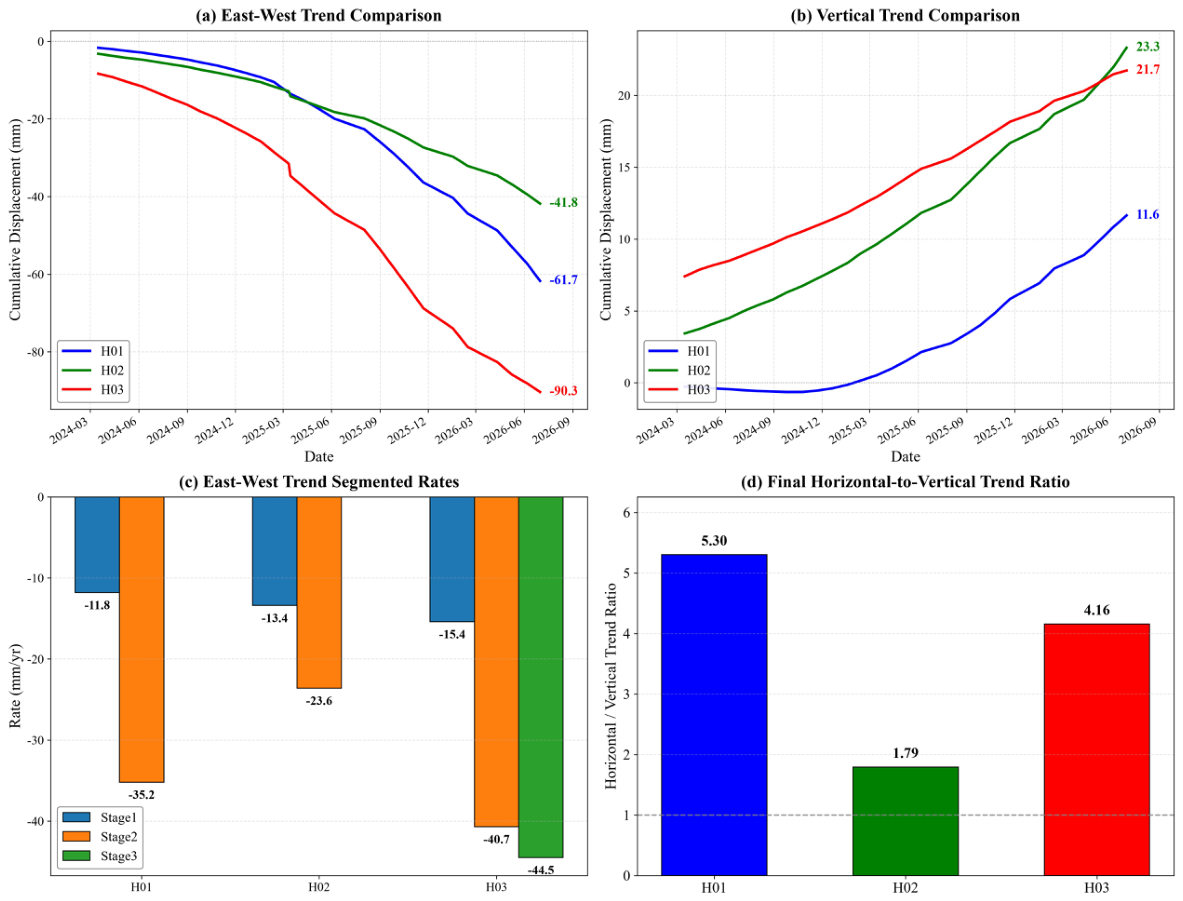
At H01 the cumulative change of the east–west trend component is mm and its variance contribution exceeds 85%, indicating that long-term creep dominates deformation in this area. The trend shows clear two-stage acceleration. The mean rate from March 2024 to March 2025 is mm/yr, rising sharply thereafter to mm/yr from March 2025 to March 2026. This is consistent with a progression from near-steady creep (the secondary stage of the classical classification) towards accelerating creep (the tertiary stage), and with an increasing reactivation hazard. The classification is not established by the trend alone: a smoothed two-year series can show an accelerating segment without the self-accelerating evolution that defines the tertiary stage, and the phrase is used here as a description of the observed trend shape. The vertical trend rises monotonically by about 11.6 mm (rate mm/yr), and its ratio to the cumulative change of the horizontal trend is about 1:5.3, confirming that the motion is dominated by horizontal pushing, while the vertical uplift may result from compressional uplift caused by undulations of the slip surface. This trend behavior agrees closely with the mechanism of “rainfall infiltration—slip-zone weakening—accelerating creep” revealed for the Daguan ancient landslide by Zhu et al. [4] on the basis of numerical simulation.
At H02 (consequent slope along the Neijiang–Kunming railway) the cumulative change of the east–west trend component is mm with a variance contribution of about 72%, so that periodic modulation is stronger. The trend shows episodic acceleration, about mm/yr in the first stage (March 2024 to June 2025) and mm/yr in the second (June 2025 to July 2026). Notably, the trend shows a short stagnation of about 2.5 mm in October–November 2025 before accelerating again, which is attributed to local locking and unlocking of the slip zone or to short-term stress adjustment caused by railway maintenance work. The vertical trend rises by a total of 23.3 mm at a rate of mm/yr (the highest of the three areas), but this rate is constant throughout the observation period and does not accelerate with the horizontal motion, forming a pattern of “horizontal acceleration with constant vertical motion”. This suggests that the dip of the slip surface may flatten as sliding proceeds, or that vertical motion is constrained by the overlying rock mass.
At H03 the east–west trend component shows the most intense and most persistently accelerating deformation in the study area, with a cumulative change of mm. The segmented rates increase continuously, about mm/yr from March to December 2024, about mm/yr from January to August 2025, and about mm/yr from September 2025 to July 2026, accelerating unidirectionally throughout without any deceleration or stagnation. It is particularly important to note that although the raw time series shows a “rebound” after February 2026 (from mm to mm), the trend component itself continues to accelerate downwards (from mm to mm), which shows that the rebound is caused entirely by the positive superposition of the periodic and noise components and must not be misinterpreted as stabilization of the deformation. The vertical trend rises gently by about 21.7 mm (rate mm/yr), and its ratio to the cumulative change of the horizontal trend is about 1:4.2, further confirming that this area is dominated by horizontal creep of a bank slope in a deeply incised valley, with a relatively stable vertical component.
Following the M 3.9 earthquake near Daguan on 12 December 2025, the trend rates at H01 and H03 both increased briefly during January–February 2026 (H01 from to mm/yr, and H03 from to mm/yr), which is a temporal coincidence of the kind that shaking can produce in a slope that is already creeping, and which is consistent with the dynamic response of fractured rock slopes to seismic loading [8]. It is not, however, a demonstration of triggering. The epicentral distance and focal depth of the event, and the estimated peak ground acceleration at the three sites, have not yet been quantified here (epicenter at 28.N, 103.E, focal depth 10 km, about 53 km from the study area; no strong-motion record is available to estimate the PGA), and the rate increase is of the same order as the scatter of the segmented rates themselves. A quantitative before–after comparison with a control site outside the shaking footprint would be required to separate a seismic effect from the ongoing acceleration. The H01 and H02 areas lie near residential expansion zones on the surface of the ancient landslide body, and the period of trend acceleration (after 2025) overlaps in time with the period of most intensive urban construction around the county seat. The overlap is suggestive but weakly constrained. Liang et al. [5] document the expansion of the built-up area of Daguan between 1970 and 2022, together with the slope cutting and filling associated with it, but their record ends in 2022 and therefore cannot document construction activity during 2024–2026. Construction records for the monitoring period (location, timing, scale and intensity of cutting and filling) are not available to us, and no maintenance record for the Neijiang–Kunming railway section has been obtained; in their absence the association between construction and the observed acceleration is reported as a temporal coincidence consistent with the mechanism proposed by Liang et al. [5], and not as evidence that construction caused the acceleration. The same reservation applies to the interpretation of the stagnation at H02 in October–November 2025 as a stress adjustment related to railway maintenance: no maintenance record has been obtained. The trend analysis shows that the H03 area is in a stage of continuously accelerating non-steady creep with the highest failure hazard and should be the core target for densified monitoring and disaster-prevention planning. The H01 area shows an accelerating trend consistent with the onset of the tertiary stage and warrants close attention during the rainy season and after felt earthquakes, although the evidence does not yet establish a stage transition (Section 4.2). The deformation mechanism of the H02 area is complex, requiring dedicated monitoring in combination with groundwater levels and engineering activity.
3.8. Periodic Component and Response to Meteorological Factors
This section compares systematically the response of the east–west (E–W) and vertical (UD) deformation components at the H01, H02 and H03 monitoring points to rainfall and maximum air temperature, using the periodic deformation components obtained from the SSA decomposition. The study period runs from 16 March 2024 to 1 July 2026. The InSAR series were interpolated linearly onto a daily grid so that they could be aligned with the daily meteorological record, which yields 838 daily values; these values are not independent observations, because they are generated by interpolation between acquisitions separated by 4–12 days (Section 2.7). The analysis methods are contemporaneous Pearson correlation, cross-lag correlation analysis over lags of 0–800 days (801 lags per series pair, without multiple-comparison correction) and cumulative scatter regression. Two consequences of this design are stated at the outset and apply to every coefficient below. First, all three series are strongly autocorrelated and seasonal, so the nominal significance levels associated with n = 838 are far too optimistic; with an effective sample size of the order of the number of independent seasonal cycles in the record, only coefficients well above the nominal 5% critical value should be regarded as resolved. Second, a search over 801 lags will produce large coefficients by chance even for unrelated series, so the lag of maximum is reported as a descriptive quantity and not as an estimated response time. The coefficients in Table 8 and in the text are therefore read as measures of the strength of association between the decomposed components and the meteorological variables, not as tests of a physical response.
Table 8.
Correlation statistics between the periodic deformation components and meteorological factors.
3.8.1. Response Characteristics of the East–West Component
The east–west periodic deformation at all three monitoring points correlates significantly and positively with maximum air temperature. The contemporaneous correlation coefficients at H01, H02 and H03 are 0.364, 0.439 and 0.466 respectively, indicating that higher temperatures are generally accompanied by larger east–west periodic deformation, so that the two vary broadly in phase on the intra-annual scale. As the amplitude of the deformation fluctuation increases, the contemporaneous correlation strengthens slightly. H03-EW has the largest standard deviation, 6.40 mm, and the strongest contemporaneous response to temperature.
By contrast, the contemporaneous correlation between rainfall and east–west deformation is generally weak. The coefficients for H01-EW and H02-EW are and , both close to zero, while H03-EW is statistically significant but has a coefficient of only 0.084, implying limited explanatory power. This indicates that rainfall makes only a weak direct contemporaneous linear contribution to the east–west periodic deformation.
The cross-lag analysis shows that the best lag for temperature is clustered around 529 days, 549 days at H01 and 529 days at both H02 and H03, all with a relatively strong negative correlation, the maximum absolute coefficient ranging from 0.651 to 0.803 and being strongest for H03-EW. Given that the total data length is only 838 days, about 529 days is equivalent to approximately 1.45 annual cycles. This result is therefore more likely to reflect the combined influence of the seasonal cycle, the trend component and the phase difference within a limited time window than a physical response time, and it is not interpreted as an actual causal lag of about one and a half years between temperature and deformation. We report it because it appears in the cross-correlation function, not because it constrains the thermal response of the slope.
The best lags for rainfall are more scattered, and they are not interpreted as response delays. H02-EW and H03-EW reach maximum correlation at about 340 and 339 days respectively, with coefficients of about 0.43 and 0.42, whereas H01-EW reaches its maximum at 793 days, which is within 45 days of the record length. At such lags the two series overlap for only a small fraction of their length, the coefficient is dominated by the few points near the series boundary, and the estimate is dominated by edge effects rather than by a physical lag. A lag of about 340 days is in turn indistinguishable from one annual cycle, which is the period at which both series are strongly autocorrelated. Neither peak survives a multiple-comparison correction appropriate to 801 tests. The scatter of the best lags between sites (339, 340 and 793 days) is itself an indication that no single, stable delay characterizes the rainfall–deformation relation in this dataset, and we therefore conclude only that the seasonal band of the east–west deformation is not explained by contemporaneous rainfall.
The cumulative regressions are reported for completeness, but they do not measure explanatory power and we do not interpret them as such. Regressing one cumulative series on another cumulative series that also increases monotonically with time tends to produce a high even when the underlying increments are independent, because both variables share the same trend; the coefficients in Table 8 are therefore inflated by construction, and the ranking of cumulative temperature above cumulative rainfall is a property of the two cumulative curves rather than of the two physical drivers. For the same reason, the negative slopes reported for all regressions cannot be read as a negative physical response: with the trend removed, the residual increments are not significantly related to the increments of either driver (the increment regression was not computed, so this statement is based on the visual absence of a stable slope in the detrended scatter rather than on a fitted model). We retain these panels because they are part of the analysis that was performed, but the inference in this paper rests on the contemporaneous coefficients and on the wavelet coherence structure, not on the cumulative regressions.
The corresponding panel plots are given in Figure 9 for H01-EW, Figure 10 for H02-EW and Figure 11 for H03-EW, each showing the three-axis time series (rainfall, temperature and deformation), the cumulative scatter regressions, the cross-correlation functions and the wavelet coherence spectra.
Figure 9.
Relationship between the east–west periodic deformation component and meteorological factors at H01. (a) Three-axis time series of rainfall, maximum temperature and deformation; (b) cumulative scatter regressions of deformation against cumulative rainfall and cumulative maximum temperature; (c) cross-correlation functions with rainfall (blue) and maximum temperature (red), the horizontal axis being the lag in days for which the meteorological variable leads the deformation; (d) cross-wavelet power spectra and wavelet coherence spectra. In (d) the thin pale contours delimit the 95% confidence region against a red-noise background, the U-shaped curve marks the cone of influence (regions outside it are affected by edge effects and are not interpreted), and the arrows give the relative phase (right: the two series are in phase; left: anti-phase; down: the deformation lags the factor by ). Panels (b,c) are descriptive and are not used for inference (Section 3.8); the interpretation rests on the coherence structure and the phase arrows in (d).
Figure 11.
As in Figure 9, but for H03 (east–west component).
3.8.2. Response Characteristics of the Vertical Component
The vertical deformation shows pronounced differences between the monitoring points, and its meteorological response is not uniform.
The H01-UD deformation is the most stable, with a mean of 0.014 mm and a standard deviation of only 0.296 mm. Its contemporaneous correlation coefficients with rainfall and maximum temperature are 0.134 and 0.121 respectively. Although statistically significant, the correlations are weak. The values of the cumulative rainfall and cumulative temperature regressions are only 0.0004 and 0.017, indicating that cumulative meteorological effects have very little explanatory power for the vertical periodic deformation at H01. Its trend slope is 0.00018 mm/d with an of 0.020, so the long-term trend is also weak. The variation of H01-UD may therefore be governed mainly by local disturbance, residual noise or unidentified factors.
H02-UD correlates significantly and negatively with maximum temperature, with a contemporaneous coefficient of that reaches a maximum negative correlation of at a lag of 283 days. Its long-term trend is upward, with a slope of 0.0013 mm/d, but the trend is only 0.036 and its explanatory power is limited. The cumulative rainfall and cumulative temperature regression values for H02-UD are 0.041 and 0.061 respectively, both low, indicating that although a degree of temperature dependence exists in the vertical response, the cumulative effect is not pronounced. The corresponding panel plot for H02-UD shows the weak contemporaneous rainfall response, the negative temperature correlation and the long-lag correlation peak at about 283 days.
H03-UD responds most strongly to maximum temperature. Its contemporaneous coefficient is 0.648 and reaches a maximum positive correlation of 0.722 at a lag of 19 days, indicating that the vertical periodic deformation at this point has a strong short-term synchronous or near-synchronous relationship with maximum temperature. H03-UD also correlates positively with rainfall contemporaneously, with a coefficient of 0.249, but becomes negatively correlated at a lag of 793 days. Because this lag approaches the sample length, boundary effects may be strong and the result should be interpreted with caution. The cumulative regression values for H03-UD do not exceed 0.014, and the long-term trend slope is mm/d with an of 0.021, showing that the strong contemporaneous temperature correlation does not translate into a pronounced long-term cumulative effect.
Overall, the vertical deformation can be summarised as follows. The response is weak and stable at H01, shows a negative temperature correlation with a long phase difference at H02, and shows a strong, rapid positive response to high temperature at H03. This difference indicates that vertical deformation may be significantly modulated by local lithology, fracture structure, groundwater recharge conditions and surface loading, rather than representing a single regional thermo-elastic response.
The corresponding panel plots are given in Figure 12 for H01-UD, Figure 13 for H02-UD and Figure 14 for H03-UD, each showing the three-axis time series, the cumulative scatter regressions, the cross-correlation functions and the wavelet coherence spectra.
Figure 12.
Relationship between the vertical periodic deformation component and meteorological factors at H01, with panels as in Figure 9.
Figure 13.
Relationship between the vertical periodic deformation component and meteorological factors at H02, with panels as in Figure 9.
Figure 14.
Relationship between the vertical periodic deformation component and meteorological factors at H03, with panels as in Figure 9.
4. Discussion
4.1. Advantage of L-Band SAR in Vegetated Mountainous Terrain
The most conspicuous quantitative result of this study is the difference in coherent-point density between the two missions. Within vegetated, non-urban terrain the ascending LT-1 stack achieved a density 42.22 times that of Sentinel-1 ( versus , an improvement of 4122.3%), and the descending stack achieved a 22.87-fold improvement (2186.9%). The dominant control on this difference is wavelength: with a radar wavelength 4.2 times longer, the L-band signal decorrelates more slowly in a canopy, and the effect is amplified in this terrain because the vegetated slopes are also the steepest and the most frequently re-worked by cultivation. The comparison is nevertheless not controlled (Section 2.2), so the numbers are reported as the performance actually obtained with these two stacks rather than as an isolated measurement of the wavelength effect. The C-band signal of Sentinel-1 (5.6 cm) is strongly attenuated and decorrelated by the canopy and by the rapid change in scatterer geometry that vegetation causes between acquisitions, whereas the L-band signal of LT-1 (23.7 cm) penetrates the canopy to interact with larger, more temporally stable elements such as trunks, branches and the ground surface. The result is a longer temporal coherence and hence a denser and more persistent measurement network. The improvement is greater in the ascending geometry (4122.3%) than in the descending one (2186.9%), which is consistent with the two geometries sampling different slope aspects and hence different vegetation and illumination conditions within this deeply dissected terrain.
The finding that matters for hazard work is not the size of the ratio but what the additional points make possible. Three consequences are specific to the present dataset and are not implied by the general coherence argument. First, the gain is concentrated where the hazard is: the C-band stacks retain only and in the non-urban (cropland and forest) class, which is the class that contains the upper parts of the slopes at H01 and H03, so that a C-band-only survey would have sampled those slopes too sparsely to establish the spatial continuity used as a delineation criterion in Section 3.3. Second, the density gain changes the geometry of the comparison itself: with 270,253 points, the LT-1 ascending stack provides enough points to match 49 significant-deformation points against Sentinel-1 within 10 m, which is the comparison that exposes the 15.32 mm/yr RMSE discussed below; a sparser stack would not have supported even that test. Third, the urban area inside the ancient landslide body is precisely where C-band coherence is least affected by vegetation and most affected by construction change, so the two missions fail for different reasons in different parts of the same study area, and their combination is more informative than either alone. Beyond these points we do not claim a new physical insight from the density comparison, and we have removed the framing that presented the percentage increase as a result in its own right.
The practical consequence is important for hazard screening. A wide-area survey based on C-band alone would leave the steep, vegetated slopes that dominate Daguan County poorly sampled, and it is precisely on such slopes that the hazard sites identified here are located. The near-continuous coverage obtained from L-band, by contrast, permits the spatial continuity of the deformation field to be assessed directly, which was one of the criteria used in Section 3.3 to delineate H01–H03. This is consistent with the advantages reported for LT-1 in large-deformation landslide monitoring and in early hazard identification.
At the same time, the cross-mission comparison at significant-deformation points returns correlation coefficients of only 0.674 (ascending) and 0.623 (descending). These values are consistent with the published performance of cross-band comparisons in steep, vegetated terrain and should be interpreted with care. The two datasets differ in wavelength, incidence angle, azimuth angle and acquisition dates, so that even a perfect measurement of the same physical displacement field would not produce identical LOS projections. The much smaller RMSE in the descending comparison (2.72 mm/yr, against 15.32 mm/yr ascending) suggests that where a larger number of point pairs is available (108 versus 49) the two missions agree more closely in rate, and that the larger ascending RMSE is at least partly a sampling effect associated with the smaller matched sample. Part of it is not: with 49 pairs, a single outlier displaces the RMSE substantially, and we have not been able to test the residual distribution because the matched pairs are too few to support a stable estimate. The two missions should therefore be regarded as corroborating rather than duplicating one another. Sentinel-1 provides a longer historical baseline and a well-characterized C-band response, while LT-1 provides the spatial completeness required in vegetated terrain.
4.2. Dominance of Horizontal Motion and Its Implications for Failure Mechanism
The two-dimensional decomposition indicates that the resolved deformation at all three sites is dominated by horizontal, east–west motion, with horizontal-to-vertical trend ratios of 5.30 (H01), 1.79 (H02) and 4.16 (H03). These ratios are computed from the end values of the SSA trend components (Table 7) and are apparent ratios in the sense of Section 2.5: they describe the part of the displacement field that the two lines of sight can resolve, and they would change if a non-negligible north–south component were present. The vertical motion is weak in absolute terms (rates of to mm/yr) and, importantly, is directed upward at all three sites. Upward vertical motion accompanying westward horizontal displacement is not compatible with simple vertical settlement. It indicates that the displacement vector lies close to the slope surface, and that the small vertical component is a geometric consequence of sliding along an inclined slip surface rather than a genuinely independent mode of deformation. The upward sign is most plausibly explained either by the arching or compressional effect produced as a slope body moves into a constraining toe, or by undulations of the slip surface.
Two checks bound the effect of the unresolved north–south component. First, a quantitative check was performed on the conditioning of the projection matrix formed from the angles in Table 3. The two lines of sight are nearly anti-parallel in azimuth (259. ascending against 101. descending), so that is poorly conditioned: its off-diagonal entry is 0.162 and its determinant is , which makes the inversion unstable with respect to . Specifically, the correction term , with , evaluates to in the east–west component and in the vertical component. This means that a north–south motion of, say, 5 mm would be aliased into about mm of apparent east–west rate and 15 mm of apparent vertical rate; the east–west component is therefore almost entirely unconstrained by the present two-geometry design. Second, a comparison of the local slope aspect with the inferred east–west direction was not performed, because a slope-aspect grid was not available for the three sites; this comparison, together with a third viewing geometry, would be required to bound empirically. These two results are reported as a limitation of the decomposition rather than corrected for, because cannot be estimated from two geometries alone.
The variation in the horizontal-to-vertical ratio between the sites is informative. H02 has by far the smallest ratio (1.79) and the largest absolute vertical rate ( mm/yr), which implies a steeper slip surface or a larger dip component of the displacement vector. This is consistent with the geological setting. H02 lies on a consequent slope developed in interbedded sandstone, shale and mudstone, where sliding is controlled by the bedding planes, which dip more steeply than the basal rupture surface of an ancient landslide. The uniform vertical rate at H02, which does not accelerate even when the horizontal rate does, further suggests that the vertical motion is governed by a structural constraint, that is, by the geometry of the bedding, rather than by the same driving process that controls the horizontal acceleration. H01 and H03, by contrast, have high ratios (5.30 and 4.16), implying shallow-dipping slip surfaces along which near-horizontal displacement is strongly favoured. For an ancient landslide accumulation body such as that at H01, and for the river-valley bank slope at H03, this geometry is the expected one.
4.3. Candidate Drivers: Temperature, Rainfall, Earthquakes and Engineering Activity
The correlation analysis yields a result that differs from the conventional expectation for rainfall-triggered landslides in Southwest China, namely that the east–west periodic deformation correlates consistently and significantly with maximum air temperature at all three sites (, 0.439 and 0.466) but only weakly with rainfall contemporaneously ( to 0.084). The best rainfall lags are also scattered between 339 and 793 days, which is inconsistent with a single, stable hydrological response time and, at the longer end, lies close to the boundary of the 838-day record, where the correlation is not well constrained. Cumulative temperature also explains more of the variance in cumulative deformation than cumulative rainfall at every site, reaching at H02-EW.
Three considerations bear on the interpretation of this pattern, and all of them argue for caution. First, the periodic component analyzed here is the seasonal band isolated by SSA, from which the long-term trend has been removed. It therefore represents the reversible part of the deformation and not the accumulating damage that ultimately leads to failure. A weak correlation with rainfall in the seasonal band does not mean that rainfall is unimportant for the long-term trend. The trend analysis in Section 3.7 shows clearly that all three sites are progressively losing stability. Second, at the intra-annual scale temperature and rainfall are strongly covarying in this monsoon climate, since the rainy season coincides with the warm season. A contemporaneous correlation with temperature may therefore partly reflect a rainfall-driven process, and the two drivers cannot be separated by contemporaneous correlation alone. Third, the very long best lags for temperature (529–549 days) are close to 1.45 annual cycles and are unlikely to represent a physical response time. They more probably arise from the interaction between the seasonal cycle, residual trend and phase difference within a limited record. The wavelet coherence analysis shown in Figure 9, Figure 10, Figure 11, Figure 12, Figure 13 and Figure 14 is more informative in this respect, because it identifies the time–frequency windows in which the two series are genuinely coherent rather than assuming a single global lag.
Two candidate near-surface mechanisms are consistent with the observed pattern, although neither can be confirmed with the data available. In the near surface, thermal cycling of the soil and rock mass produces thermo-elastic strain and, where seasonal freezing occurs, freeze–thaw effects. Both would operate with little or no lag and would produce a short-lag, in-phase relationship of the kind observed at H03-UD, where the correlation with maximum temperature is 0.648 contemporaneously and peaks at 0.722 at a lag of only 19 days. The freeze–thaw interpretation, however, remains a possibility rather than a result: no ground temperature, soil temperature, freezing index, snow-cover or frost-depth observation is available for the site, and correlations with air temperature alone cannot distinguish thermal strain from freeze–thaw. The mean annual temperature of the area is about C and the extreme minimum is ∘C, so seasonal freezing of the shallow subsoil is possible at the elevations of the county seat, but this has not been documented at the monitoring points. Establishing it would require a ground-temperature record at the sites or a freezing-index map for the county. The recurrence of noise peaks each April at H02, which the SSA decomposition isolates as anomalous residual ( and mm), is a further indication of a seasonal thermal or freeze–thaw control, since April is the month in which the shallow subsoil in this region thaws and groundwater recharge begins. The alternative, hydrological, mechanism—infiltration, pore-pressure rise and slip-zone softening—is a deeper process with a lag that depends on the hydraulic conductivity and thickness of the unsaturated zone, and its signature should appear in the trend rather than the seasonal band.
The episodic accelerations identified in the SSA trend components are temporally coincident with external events, although the evidence that they were triggered by those events is indirect (Figure 8c and Section 3.7). The M 3.9 earthquake of 12 December 2025 was followed within weeks by a brief increase in trend rate at H01 (from to mm/yr) and at H03 (from to mm/yr) during January–February 2026. A moderate earthquake would not be expected to initiate failure in a stable slope, but dynamic shaking can raise pore pressures, remobilize the slip zone and reduce the effective stress in a slope that is already creeping, so that a step-like rate increase in an already accelerating slope is a physically possible response. That the response was transient, with the rates subsequently relaxing, is also consistent with a triggering rather than a causative role. The case is nonetheless circumstantial: the epicentral distance, focal depth and estimated peak ground acceleration at the sites have not been quantified (epicenter at 28.N, 103.E, focal depth 10 km, about 53 km from the study area; no strong-motion record to estimate the PGA), no co-seismic displacement is resolved, and the rate change is comparable to the scatter of the segmented rates. We therefore report the earthquake as one candidate driver acting on a slope that was already accelerating, not as the cause of the acceleration. The coincidence of the acceleration stage at H01 and H02 with the period of peak urban construction and slope cutting around the ancient landslide body points to a second candidate driver of anthropogenic origin, for which the evidence is weaker still, because the construction history of the monitoring period has not been documented (Section 3.7). Slope cutting at the toe removes the resisting mass and fill loading at the head adds driving stress, so that the observed acceleration is consistent with the relationship between urban expansion and enhanced slope deformation reported by Liang et al. [5]. The short stagnation of about 2.5 mm observed in the H02 trend during October–November 2025, followed by renewed acceleration, may similarly reflect a locking–unlocking cycle of the slip zone or a temporary stress adjustment associated with railway maintenance.
4.4. Implications for Monitoring and Early Warning
The three hazard sites require different monitoring strategies, and the signal decomposition carried out here provides the basis for distinguishing them. H03 has the highest relative priority of the three sites, on the basis of deformation intensity alone, and should be treated as the core target for densified monitoring. Its east–west trend accelerates continuously and without interruption ( to mm/yr), its cumulative trend displacement is the largest in the study area ( mm), and its periodic amplitude of 30.46 mm is approximately four times that of the other sites. The last of these is of particular operational importance. The apparent rebound of about 15 mm between February and July 2026 in the raw time series might be read as a sign that the slope had stabilized, whereas the trend component continues to accelerate throughout the same interval. Any early-warning system based on raw cumulative displacement would therefore risk a false negative at precisely the site where the consequences would be most severe. Monitoring at H03 should be based on the trend component rather than on the raw series.
H01 shows an accelerating trend, with a two-stage increase in rate from to mm/yr. We describe this as consistent with the onset of the tertiary stage rather than as an established transition: the classical criteria for that stage require a progressive, self-accelerating velocity evolution, and a smoothed two-year series can indicate such a trend but cannot demonstrate it. Operationally, however, the distinction matters little: a site whose rate has tripled within a year warrants the same precautions as one that has formally entered the tertiary stage. The practical implication is that H01 should be closely watched during the rainy season and in the aftermath of any felt earthquake. H02 presents the most complex case. Its mechanism is bedding-controlled, its deformation is modulated by engineering activity and railway maintenance, and its slip zone appears to alternate between locked and unlocked states. Effective monitoring at H02 would need to be combined with groundwater observations and with records of construction and maintenance activity, since without those the deformation signal cannot be fully explained by the data used here.
From a methodological standpoint, the results support two broader recommendations. First, L-band data should be the primary source for wide-area hazard screening in the densely vegetated mountains of Southwest China, with C-band data used to extend the historical baseline and to provide an independent check on rate estimates. Second, the separation of deformation into trend and periodic components should be treated as a routine step in operational monitoring rather than an optional analysis, because the two components carry different information. The trend carries the irreversible loss of stability that determines the time to failure, while the periodic component carries the reversible response that determines when a slope may be temporarily weakened. Confusing the two can lead to an incorrect assessment of stability in either direction, as the H03 record demonstrates.
4.5. Limitations and Future Work
Several limitations should be acknowledged. First, the deformation observations are restricted to the line of sight of a single pair of geometries, so that the north–south component is not resolved. Given that the dominant motion at these sites is east–west, this is not a serious constraint for the kinematic interpretation presented here, but it means that the full three-dimensional displacement field cannot be recovered, and in particular that any along-slope component with a strong north–south orientation would be missed. Second, the two-dimensional decomposition is based on the standard assumption of a rigid, planar surface with a single incidence angle per track. In terrain as steep as this, local incidence angles vary substantially, and a more rigorous decomposition would use local rather than nominal angles. Third, the analysis contains no geotechnical information, as borehole data, slip-surface depths and material properties are unavailable. The hazard-level judgement in this study is therefore semi-quantitative and based on expert judgement, and should be regarded as a preliminary screening rather than a quantitative risk assessment.
Four further limitations follow from the design of the study and should be weighed when the results are used. First, there is no independent validation of the InSAR displacements. No GNSS, leveling, total-station, crack-meter or extensometer data were available for the three sites during the monitoring period, so the accuracy of the rates rests on the internal consistency of the processing and on the cross-mission comparison of Section 3.2, neither of which is an external check. This matters most where millimeter-scale changes are interpreted: the difference between the trend and the seasonal component at H03, on which the rebound argument depends, is of the same order as the uncertainty that a validation campaign would be expected to quantify. Second, the 10 mm/yr threshold used to define significant deformation is an empirical choice, but it is a defensible one, and we justify it here rather than treat it as a free parameter. The 15.32 mm/yr RMSE of the ascending cross-mission comparison is a between-sensor quantity: it measures the difference between two LOS projections that differ in wavelength, incidence and azimuth angle, and acquisition date, so it is not the uncertainty of a single rate and should not be used as an error floor for the threshold. The relevant quantity is the spread of a single dataset: over the full LT-1 descending stack (686,378 points) the standard deviation of the LOS rate is 4.55 mm/yr, so that 10 mm/yr corresponds to about 2.2 standard deviations and lies just above the 99th percentile of the rate distribution (9.25 mm/yr); a point above 10 mm/yr is therefore an extreme outlier relative to the noise floor rather than part of it. A sensitivity analysis over the study area (156,453 points) confirms that this choice sits at the elbow of the count curve: the proportion of points above the threshold falls from 34.6% at 5 mm/yr to 4.98% at 10 mm/yr, 0.87% at 15 mm/yr and 0.07% at 20 mm/yr. A 5 mm/yr threshold would flood the map with noise-dominated points, while 20 mm/yr is so stringent that the moderately deforming site H02—whose rate range is to mm/yr—loses essentially all of its points; H01 and H03, which deform faster, remain robustly identified down to the 15 mm/yr level. The three sites are therefore stable over the range 10–15 mm/yr, and 10 mm/yr is retained as a balance between missed and false detections. Third, the hazard sites are identified from deformation anomalies and from their coincidence with the mapped ancient landslide boundary, not from field evidence of active movement, and the elements exposed are described qualitatively. No exposure, vulnerability, population, building, traffic or asset inventory was used, so no hazard or risk ranking is implied by the ordering of H01–H03, and terms such as “highest potential hazard” have been replaced by statements about relative monitoring priority. Fourth, the SSA decomposition, on which much of the interpretation rests, depends on the window length and on the grouping of eigentriples; the settings and the sensitivity check are reported in Section 2.6, but a full sensitivity study over a range of window lengths and groupings has not been carried out, and the separation of trend from seasonal signal at the end of the record—which is where the two components most strongly oppose one another—is the part most sensitive to that choice.
5. Conclusions
This study used ascending and descending SAR imagery acquired by Sentinel-1 and by the LT-1 constellation between March 2024 and July 2026, together with DS-InSAR processing, two-dimensional decomposition, singular spectrum analysis and multi-factor correlation analysis, to identify deforming ground and to examine its association with candidate drivers around the county seat of Daguan County, Yunnan Province. The conclusions are framed accordingly: they report what was observed and what is statistically associated with it, and they distinguish these from mechanistic interpretation, which the data do not establish.
- (1)
- Wide-area LOS deformation velocity fields were successfully obtained for the county seat of Daguan and the surrounding ancient landslide body using DS-InSAR. The LOS rates range from to mm/yr for LT-1 ascending, from to mm/yr for LT-1 descending, from to mm/yr for Sentinel-1 ascending and from to mm/yr for Sentinel-1 descending. Deformation is non-uniform in space, and the high-rate zones are concentrated at the intersection of a deeply incised river valley and the ancient landslide accumulation body around 103.E, 27.N, where the significant-deformation points overlap strongly across all four tracks and the trend of the deforming zone runs roughly parallel to the local river and ridge lines.
- (2)
- The comparison between the two missions shows a clear operational advantage for the L-band data in vegetated terrain, although the comparison is not a controlled one and the advantage is not attributed to wavelength alone. In ascending mode LT-1 provided coherent points per , an increase of 2274.0% over Sentinel-1, rising to 4122.3% within vegetated areas. In descending mode the density was , an increase of 954.6% overall and 2186.9% in vegetated areas. At significant-deformation points the correlation coefficients between the two missions are 0.674 (ascending, 49 matched pairs) and 0.623 (descending, 108 pairs), with RMSE values of 15.32 and 2.72 mm/yr; this indicates moderate agreement, and the ascending RMSE exceeds the 10 mm/yr threshold used here, so the two missions corroborate rather than validate one another. The combination of the two missions nevertheless broadens the coverage available for hazard screening in vegetated mountainous terrain, most of all on the vegetated slopes where the C-band point density falls below .
- (3)
- On the basis of a rate threshold of mm/yr combined with time-series shape, spatial continuity and the existing inventory, three typical hazard sites were delineated within the county seat area: H01 ( to mm/yr, ), H02 ( to mm/yr, ) and H03 ( to mm/yr, ). All three lie within the mapped extent of the ancient landslide body and coincide closely with it, which supports—but does not confirm—their interpretation as active slope deformation; field verification of the three sites has not yet been carried out. The result nevertheless indicates the value of wide-area MT-InSAR monitoring as a complement to manual field survey in terrain that is difficult to access.
- (4)
- Two-dimensional decomposition shows that deformation at all three sites is dominated by near-horizontal east–west motion with weak vertical motion. The mean east–west rates are mm/yr at H01 (92.9% significant-deformation points), mm/yr at H02 and mm/yr at H03 (77.3% significant-deformation points), with a peak rate of mm/yr at H03. The horizontal-to-vertical trend ratios are 5.30, 1.79 and 4.16, the smallest ratio occurring at H02, where the steeper dip of the bedding-controlled slip surface is reflected in the largest absolute vertical rate ( mm/yr).
- (5)
- SSA decomposition separates the deformation series into trend, periodic and residual components whose behavior differs systematically between the three sites. At H01 the east–west trend has a cumulative displacement of mm and its rate increases in two stages from to mm/yr, a pattern consistent with a transition from near-steady to accelerating creep. At H02 the cumulative trend displacement is mm and acceleration is episodic, including a stagnation of about 2.5 mm, while the vertical trend rises by 23.3 mm at a constant rate. At H03 the trend displacement reaches mm and accelerates continuously to mm/yr. The periodic amplitude at H03 is 30.46 mm, roughly four times that of the other sites. It reproduces most of the apparent rebound of about 15 mm in the raw series after February 2026, so that rebound is not evidence that the slope has stabilized: the displacement itself is real, but under the adopted decomposition it belongs to the seasonal component, while the trend continues to accumulate.
- (6)
- The east–west periodic deformation correlates significantly and positively with maximum air temperature at all three sites (, 0.439 and 0.466), whereas its contemporaneous correlation with rainfall is weak and its best rainfall lags are scattered between roughly 339 and 793 days. Cumulative temperature explains more of the variance in cumulative deformation than cumulative rainfall at every site, reaching at H02-EW. The vertical component at H03 shows the strongest response, with a contemporaneous correlation of 0.648 that peaks at 0.722 for a lag of only 19 days, which is consistent with a near-synchronous thermal influence in the shallow subsoil; freeze–thaw cannot be distinguished from thermo-elastic strain without ground-temperature observations, and is reported as a possible rather than an established mechanism.
- (7)
- The episodic accelerations in the trend components are temporally coincident with two external events, which we report as candidate triggers. Following the M 3.9 earthquake near Daguan on 12 December 2025, the trend rates at H01 and H03 increased briefly during January–February 2026 (H01 from to mm/yr, and H03 from to mm/yr), a coincidence consistent with an influence of ground shaking on slopes that were already accelerating, but not sufficient to establish triggering, because the source parameters and the ground motion at the sites have not been quantified. The acceleration stage at H01 and H02 also coincides with the peak period of urban construction and slope cutting on the ancient landslide body, which is consistent with an influence of cutting and filling on reactivation, although construction records for the monitoring period are not available to test it. H03 should be designated the core target for densified monitoring and disaster-prevention planning, H01 requires vigilance against sudden failure during the rainy season or following earthquakes, and H02 requires dedicated monitoring combined with groundwater and engineering-activity records.
Supplementary Materials
The following supporting information can be downloaded at: https://www.mdpi.com/article/10.3390/rs18213824/s1, Figure S1: Cross-mission agreement at significant-deformation points.
Author Contributions
Conceptualization, W.W. and Y.L.; methodology, W.W.; software, C.Z.; validation, W.W.; formal analysis, W.W.; investigation, X.Z.; resources, C.H.; data curation, C.Z.; writing—original draft preparation, W.W.; writing—review and editing, W.W.; visualization, M.D.; supervision, C.Z.; project administration, C.Z.; funding acquisition, W.W. All authors have read and agreed to the published version of the manuscript.
Funding
This research was supported in part by the Yunnan Provincial Key Research and Development Program Project under Grant 202603AG380001 and in part by the National Natural Science Foundation of China under Grants 42401547 and 42404051.
Data Availability Statement
The Sentinel-1 SAR data are available from the Alaska Satellite Facility (ASF) and the Copernicus Data Space Ecosystem. The LT-1 SAR data and the associated precise orbit products were provided by the Yunnan Institute of Geological Environment Monitoring. The TanDEM-X 30 m Edited DEM is available from the DLR EOC Geoservice. The meteorological observations were provided by the Meteorological Data Centre of the China Meteorological Administration, and the earthquake catalogue by the China Earthquake Networks Centre. The processed deformation products generated in this study are available from the corresponding author on reasonable request.
Acknowledgments
The authors thank the Yunnan Institute of Geological Environment Monitoring for providing the LT-1 SAR data and supporting data processing, the Meteorological Data Centre of the China Meteorological Administration for providing the meteorological observations, and the China Earthquake Networks Centre for providing the earthquake catalogue.
Conflicts of Interest
The authors declare no conflicts of interest.
References
- Cheng, Y.; Pang, H.; Li, Y.; Fan, L.; Wei, S.; Yuan, Z.; Fang, Y. Applications and Advancements of Spaceborne InSAR in Landslide Monitoring and Susceptibility Mapping: A Systematic Review. Remote Sens. 2025, 17, 999. [Google Scholar] [CrossRef] [Scilit]
- Zhang, Y.; Ren, S.; Wu, R.; Li, J.; Ran, L. Major Progress on Reactivation Mechanism and Early Identification of Ancient Landslides on the Eastern Tibetan Plateau. Nat. Hazards Rev. 2024, 25, NHENG-2146. [Google Scholar] [CrossRef] [Scilit]
- Liu, Z. Development Characteristics and Risk Assessment of Geological Hazards in Daguan County. Master’s Thesis, Kunming University of Science and Technology, Kunming, China, 2022. (In Chinese) [Google Scholar] [CrossRef]
- Zhu, S.; Yin, Y.; Tie, Y.; Sa, L.; Gao, Y.; He, Y.; Zhao, H. Deformation characteristics and reactivation mechanism of a giant ancient landslide in the Wumeng Mountain area: A case study of the Daguan ancient landslide. Chin. J. Geotech. Eng. 2025, 47, 305–314. (In Chinese) [Google Scholar] [CrossRef]
- Liang, J.; Zhao, C.; Zhang, S.; Dong, J.; Tie, Y.; Gao, Y.; Sa, L.; Yang, L.; Yan, S. Development and evolution characteristics of giant ancient landslide bodies in the mountainous area of Southwest China and their relationship with urban spatial expansion. Sediment. Geol. Tethyan Geol. 2024, 44, 510–522. (In Chinese) [Google Scholar] [CrossRef]
- Lacroix, P.; Handwerger, A.L.; Bièvre, G. Life and death of slow-moving landslides. Nat. Rev. Earth Environ. 2020, 1, 404–419. [Google Scholar] [CrossRef] [Scilit]
- Novellino, A.; Pennington, C.; Leeming, K.; Taylor, S.; Alvarez, I.G.; McAllister, E.; Arnhardt, C.; Winson, A. Mapping landslides from space: A review. Landslides 2024, 21, 1041–1052. [Google Scholar] [CrossRef] [Scilit]
- Jibson, R.W.; Harp, E.L.; Michael, J.A. A method for producing digital probabilistic seismic landslide hazard maps. Eng. Geol. 2000, 58, 271–289. [Google Scholar] [CrossRef] [Scilit]
- Notti, D.; Galve, J.P.; Mateos, R.M.; Monserrat, O.; Lamas-Fernández, F.; Fernández-Chacón, F.; Roldán-García, F.J.; Pérez-Peña, J.V.; Crosetto, M.; Azañón, J.M. Human-induced coastal landslide reactivation. Monitoring by PSInSAR techniques and urban damage survey (SE Spain). Landslides 2015, 12, 1007–1014. [Google Scholar] [CrossRef] [Scilit]
- Casagli, N.; Intrieri, E.; Tofani, V.; Gigli, G.; Raspini, F. Landslide detection, monitoring and prediction with remote-sensing techniques. Nat. Rev. Earth Environ. 2023, 4, 51–64. [Google Scholar] [CrossRef] [Scilit]
- Yang, F.; Shi, X.; Dai, K.; Zhang, W.; Yang, S.; Han, J.; Wen, N.; Deng, J.; Li, T.; Yao, Y.; et al. Utilizing LuTan-1 SAR Images to Monitor the Mining-Induced Subsidence and Comparative Analysis with Sentinel-1. Remote Sens. 2024, 16, 4281. [Google Scholar] [CrossRef] [Scilit]
- Ferretti, A.; Prati, C.; Rocca, F. Permanent scatterers in SAR interferometry. IEEE Trans. Geosci. Remote Sens. 2001, 39, 8–20. [Google Scholar] [CrossRef] [Scilit]
- Ferretti, A.; Prati, C.; Rocca, F. Nonlinear subsidence rate estimation using permanent scatterers in differential SAR interferometry. IEEE Trans. Geosci. Remote Sens. 2000, 38, 2202–2212. [Google Scholar] [CrossRef] [Scilit]
- Berardino, P.; Fornaro, G.; Lanari, R.; Sansosti, E. A new algorithm for surface deformation monitoring based on small baseline differential SAR interferograms. IEEE Trans. Geosci. Remote Sens. 2002, 40, 2375–2383. [Google Scholar] [CrossRef] [Scilit]
- Hooper, A.; Zebker, H.; Segall, P.; Kampes, B. A new method for measuring deformation on volcanoes and other natural terrains using InSAR persistent scatterers. Geophys. Res. Lett. 2004, 31, L23611. [Google Scholar] [CrossRef] [Scilit]
- Hooper, A.; Segall, P.; Zebker, H. Persistent scatterer interferometric synthetic aperture radar for crustal deformation analysis, with application to Volcán Alcedo, Galápagos. J. Geophys. Res. Solid Earth 2007, 112, B07407. [Google Scholar] [CrossRef] [Scilit]
- Ferretti, A.; Fumagalli, A.; Novali, F.; Prati, C.; Rocca, F.; Rucci, A. A new algorithm for processing interferometric data stacks: SqueeSAR. IEEE Trans. Geosci. Remote Sens. 2011, 49, 3460–3470. [Google Scholar] [CrossRef] [Scilit]
- Jiang, M.; Ding, X.; Hanssen, R.F.; Malhotra, R.; Chang, L. Fast statistically homogeneous pixel selection for covariance matrix estimation for multitemporal InSAR. IEEE Trans. Geosci. Remote Sens. 2015, 53, 1213–1224. [Google Scholar] [CrossRef] [Scilit]
- Ansari, H.; De Zan, F.; Bamler, R. Efficient phase estimation for interferogram stacks. IEEE Trans. Geosci. Remote Sens. 2018, 56, 4109–4125. [Google Scholar] [CrossRef] [Scilit]
- Guarnieri, A.M.; Tebaldini, S. On the exploitation of target statistics for SAR interferometry applications. IEEE Trans. Geosci. Remote Sens. 2008, 46, 3436–3443. [Google Scholar] [CrossRef] [Scilit]
- Zhao, C.; Li, Z.; Zhang, P.; Tian, B.; Gao, S. Improved maximum likelihood estimation for optimal phase history retrieval of distributed scatterers in InSAR stacks. IEEE Access 2019, 7, 186319–186327. [Google Scholar] [CrossRef] [Scilit]
- Zhao, C.; Yan, Y.; Yu, H. Coherence matrix estimation with total positivity regularization for interferometric phase linking. IEEE J. Sel. Top. Appl. Earth Obs. Remote Sens. 2025, 18, 8547–8558. [Google Scholar] [CrossRef] [Scilit]
- Zhao, C.; Yu, H.; Jiang, M. Distributed scatterer interferometry from traditional methods to deep learning: A comprehensive review. IEEE Geosci. Remote Sens. Mag. 2026, 14, 433–456. [Google Scholar] [CrossRef] [Scilit]
- Li, G.; Yu, H.; Zhao, C.; Yan, Y.; Yang, T.; Pascazio, V. A three-cornered hat-based approach for time-series InSAR accuracy assessment. IEEE Trans. Geosci. Remote Sens. 2026, 64, 3707944. [Google Scholar] [CrossRef] [Scilit]
- Cohen-Waeber, J.; Bürgmann, R.; Chaussard, E.; Giannico, C.; Ferretti, A. Spatiotemporal patterns of precipitation-modulated landslide deformation from independent component analysis of InSAR time series. Geophys. Res. Lett. 2018, 45, 1878–1887. [Google Scholar] [CrossRef] [Scilit]
- Ding, C.; Feng, G.; Liao, M.; Tao, P.; Zhang, L.; Xu, Q. Displacement history and potential triggering factors of Baige landslides, China revealed by optical imagery time series. Remote Sens. Environ. 2021, 254, 112253. [Google Scholar] [CrossRef] [Scilit]
- Liu, X.; Zhu, W.; Cheng, Y.; Wang, Y.; Li, Z.; Zhan, J.; Zhang, R.; He, Q. Integrating multi-temporal UAV and InSAR images for post-failure spatiotemporal deformation investigation of the Baige landslide, Jinsha River Basin, China. Eng. Geol. 2026, 367, 108735. [Google Scholar] [CrossRef] [Scilit]
- Guzzetti, F.; Cardinali, M.; Reichenbach, P. The AVI project: A bibliographical and archive inventory of landslides and floods in Italy. Environ. Manag. 1994, 18, 623–633. [Google Scholar] [CrossRef] [Scilit]
- Ohlmacher, G.C.; Davis, J.C. Using multiple logistic regression and GIS technology to predict landslide hazard in northeast Kansas, USA. Eng. Geol. 2003, 69, 331–343. [Google Scholar] [CrossRef] [Scilit]
- Wang, Q.; Li, W.; Yan, S.; Wu, Y.; Pei, Y. GIS-based frequency ratio and index of entropy models to landslide susceptibility mapping (Daguan, China). Environ. Earth Sci. 2016, 75, 780. [Google Scholar] [CrossRef] [Scilit]
- Wang, H.; Tie, Y.; Zhang, Y.; Wang, C.; Sa, L.; Gao, Y.; Bai, Y.; Liang, J.; Zhu, S.; Tang, P. Reactivation mechanisms of ancient landslide under the combined interactions of rainfall and top loading in Daguan County, Yunnan, China. Environ. Earth Sci. 2025, 84, 654. [Google Scholar] [CrossRef] [Scilit]
- Torres, R.; Snoeij, P.; Geudtner, D.; Bibby, D.; Davidson, M.; Attema, E.; Potin, P.; Rommen, B.; Floury, N.; Brown, M.; et al. GMES Sentinel-1 mission. Remote Sens. Environ. 2012, 120, 9–24. [Google Scholar] [CrossRef] [Scilit]
- Hanssen, R.F. Radar Interferometry: Data Interpretation and Error Analysis; Springer: Dordrecht, The Netherlands, 2001. [Google Scholar]
- Zebker, H.A.; Villasenor, J. Decorrelation in interferometric radar echoes. IEEE Trans. Geosci. Remote Sens. 1992, 30, 950–959. [Google Scholar] [CrossRef] [Scilit]
- Rosen, P.A.; Hensley, S.; Joughin, I.R.; Li, F.K.; Madsen, S.N.; Rodriguez, E.; Goldstein, R.M. Synthetic aperture radar interferometry. Proc. IEEE 2000, 88, 333–382. [Google Scholar] [CrossRef] [Scilit]
- He, W.; Zhang, Q.; Wang, Z.; Zhao, C. Assessment of Decorrelation and Deformation Monitoring Accuracy in Geosynchronous SAR Interferometry. IEEE J. Miniaturization Air Space Syst. 2025, 6, 321–328. [Google Scholar] [CrossRef] [Scilit]
- Chen, B.; Yang, J.; Li, Z.; Yu, C.; Yu, Y.; Qin, L.; Yang, Y.; Yu, H. A new sequential homogeneous pixel selection algorithm for distributed scatterer InSAR. GIScience Remote Sens. 2023, 60, 2218261. [Google Scholar] [CrossRef] [Scilit]
- Crosetto, M.; Monserrat, O.; Cuevas-González, M.; Devanthéry, N.; Crippa, B. Persistent scatterer interferometry: A review. ISPRS J. Photogramm. Remote Sens. 2016, 115, 78–89. [Google Scholar] [CrossRef] [Scilit]
- Grinsted, A.; Moore, J.C.; Jevrejeva, S. Application of the cross wavelet transform and wavelet coherence to geophysical time series. Nonlinear Process. Geophys. 2004, 11, 561–566. [Google Scholar] [CrossRef] [Scilit]
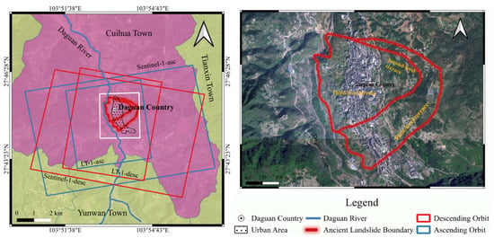
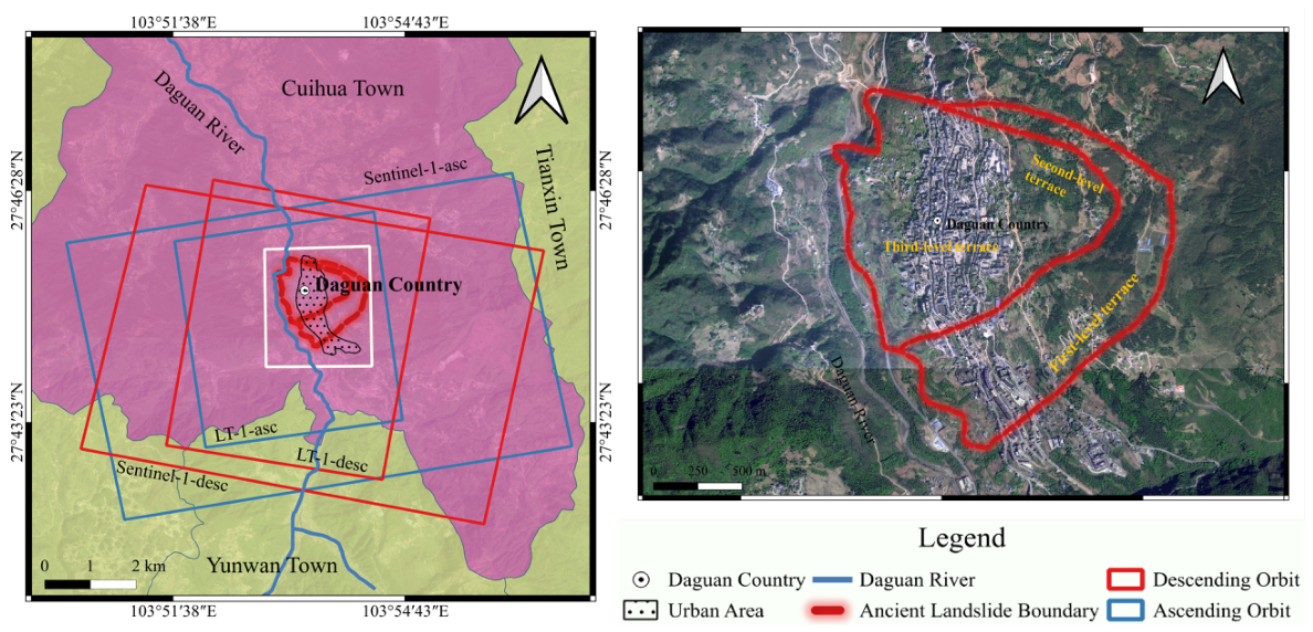
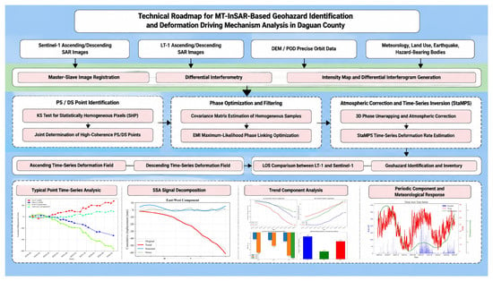
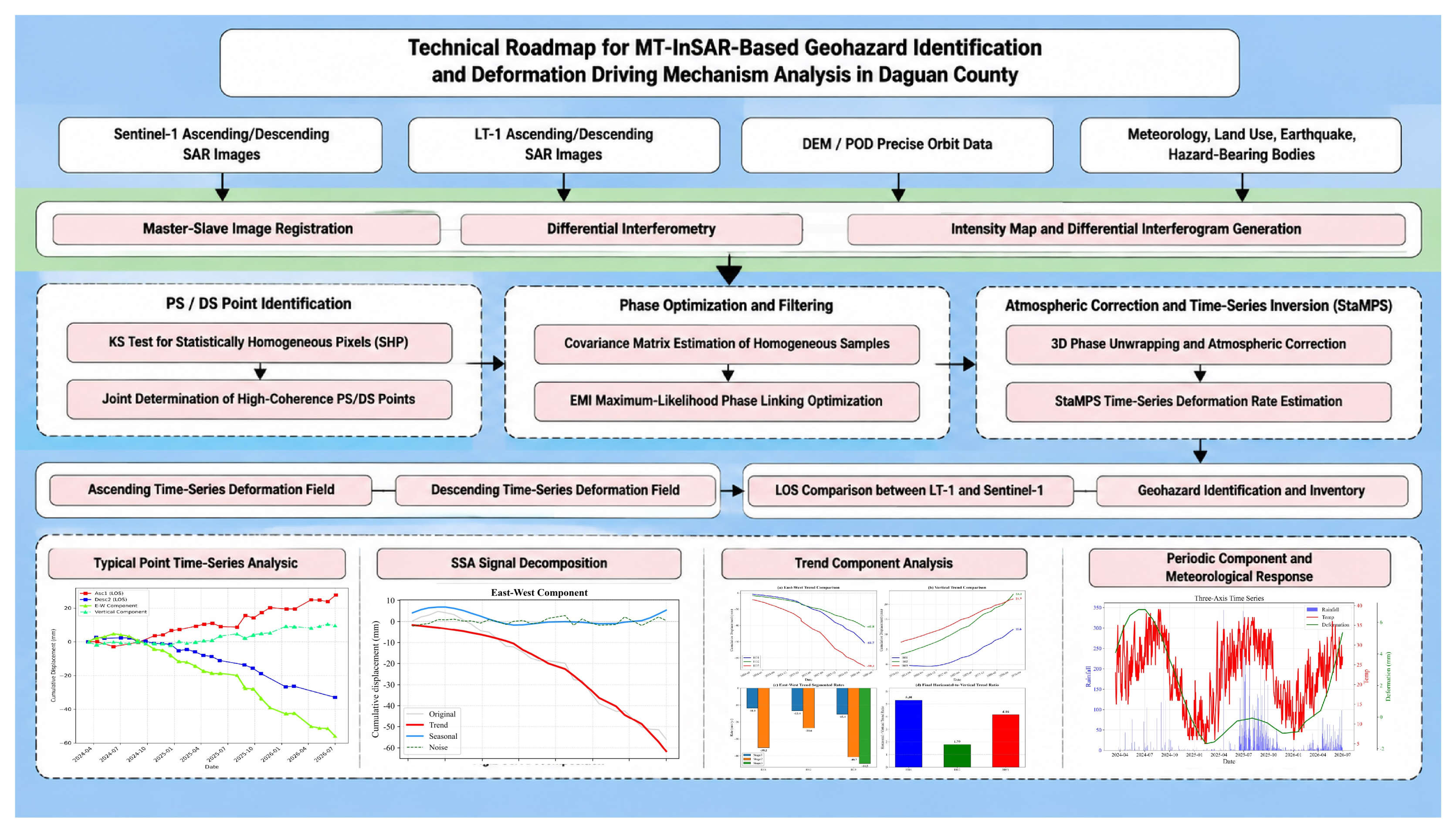
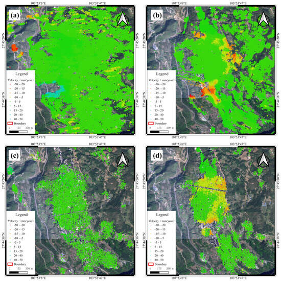
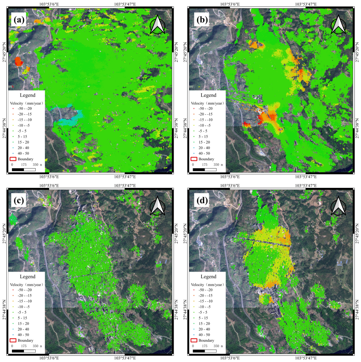
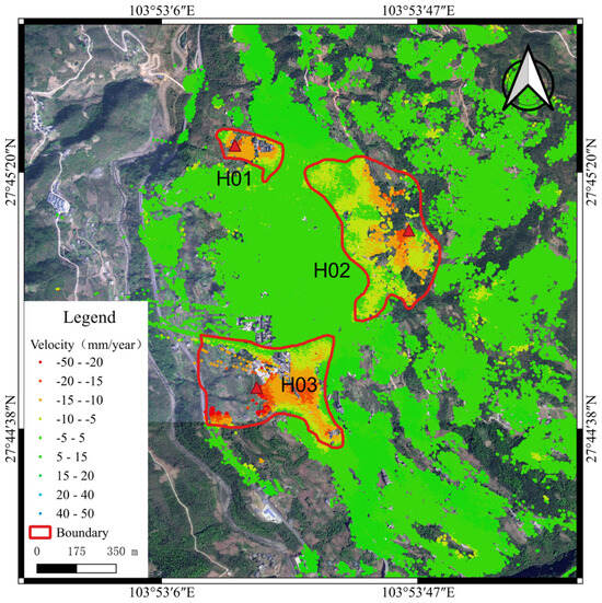
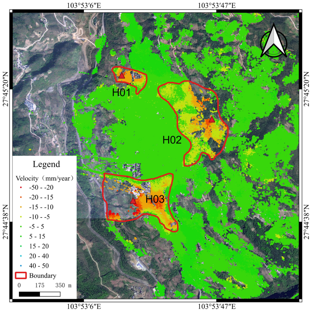
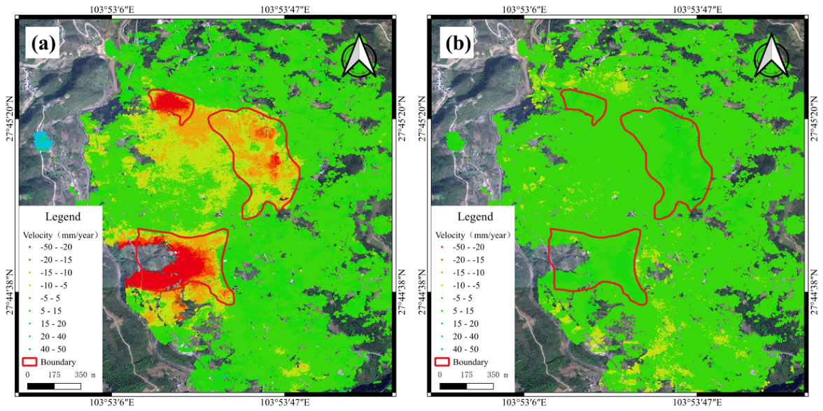
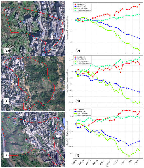
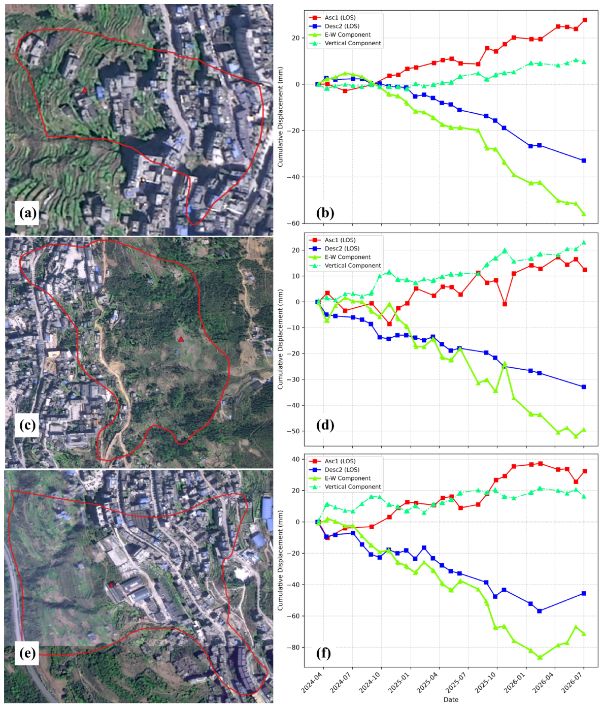
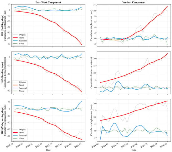
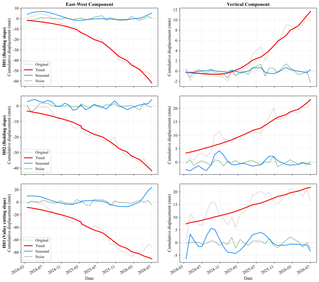
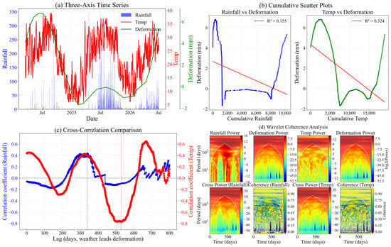
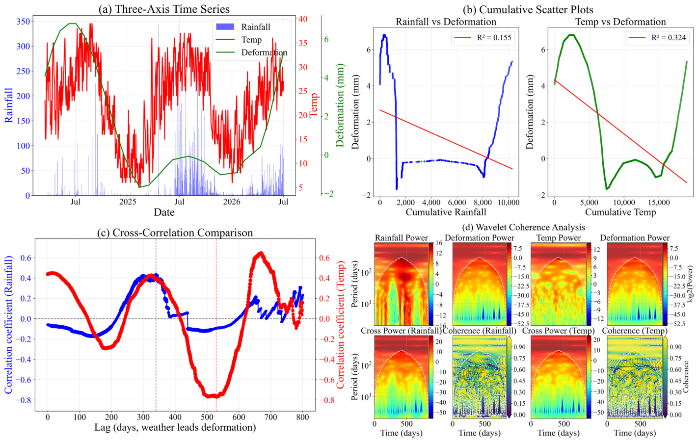
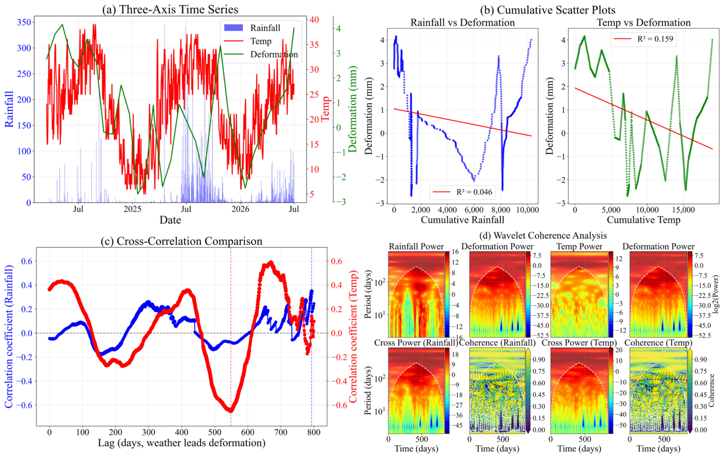
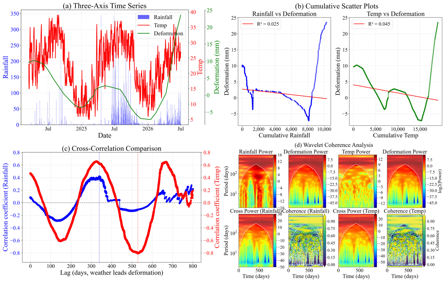
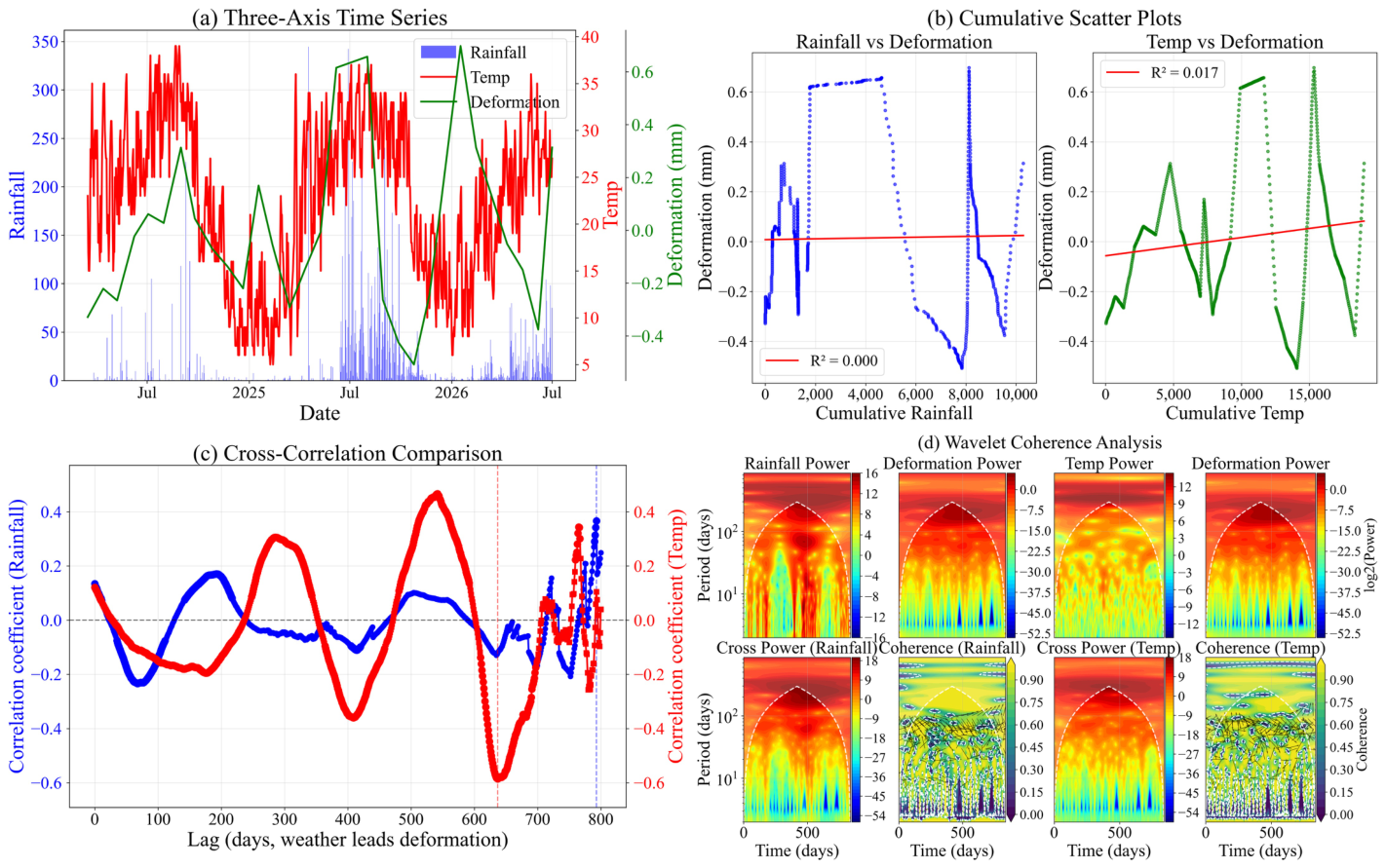
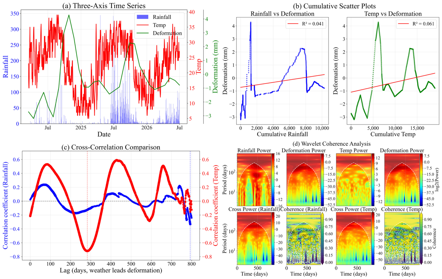
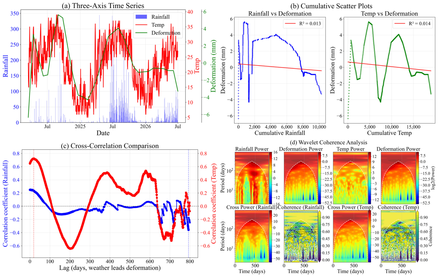

Disclaimer/Publisher’s Note: The statements, opinions and data contained in all publications are solely those of the individual author(s) and contributor(s) and not of MDPI and/or the editor(s). MDPI and/or the editor(s) disclaim responsibility for any injury to people or property resulting from any ideas, methods, instructions or products referred to in the content. |
© 2026 by the authors. Licensee MDPI, Basel, Switzerland. This article is an open access article distributed under the terms and conditions of the Creative Commons Attribution (CC BY) license.