SparseHSR: From RGB Guidance to Sparse Visible–NIR Sensing for Full-Range Hyperspectral Super-Resolution

Highlights

What are the main findings?

• Adding one high-resolution NIR band at 801 nm to RGB reduced full-spectrum mean per-band RMSE by 92.2% on Chikusei and 75.5% on ICVL.
• A few strategically distributed visible–NIR bands supported strong full-spectrum reconstruction, while their effectiveness depended strongly on the reconstruction architecture.

What is the implication of the main findings?

• In the tested reduced-resolution fusion setting, a small set of high-resolution visible–NIR observations can support full-spectrum reconstruction; implementation-level sensor benefits remain to be established.
• The choice of sparse high-resolution bands should account for the reconstruction method; this study evaluates predefined candidate configurations rather than implementing automated sensor–algorithm co-optimization.

Abstract

Hyperspectral image (HSI) super-resolution often uses RGB or RGB-like high-resolution guidance, which provides no direct high-resolution observation in the near-infrared (NIR). Keeping the low-resolution HSI spectrally complete, we first add one high-resolution NIR band near 801 nm to RGB. For abundance-Gram reconstruction, this reduces full-spectrum mean per-band RMSE by 92.2% on Chikusei and 75.5% on ICVL. We then replace RGB with only one to four high-resolution narrowbands spanning the visible and NIR. A few strategically distributed bands support strong full-spectrum reconstruction while substantially reducing the high-resolution spectral measurement burden. Using the same sparse observations, abundance-Gram reconstruction is strongly sensitive to wavelength placement, whereas registered HySure-SVD is much less sensitive. A targeted three-seed analysis confirms that the key 549 + 801 nm and four-band spanning designs are highly stable, while some weaker configurations are seed-sensitive. A guide-permutation stress test links the cross-architecture contrast to permutation-invariant global abundance-statistics matching versus registered pixelwise fusion. Sensor-native HySpex Mjolnir imagery reproduces the same crossover. These results support sparse visible-NIR sensing and joint design of high-resolution measurements and reconstruction.

1. Introduction

A large body of hyperspectral image (HSI) super-resolution and spectral-reconstruction work is built around RGB or RGB-like high-resolution guidance, and many of its most-used benchmarks live almost entirely in the visible range [1,2,3]. More general HSI–multispectral fusion formulations allow richer guidance, yet they still treat the high-resolution observation as a fixed acquisition modality rather than something to be designed [4,5]. This convention hides a simple problem: the moment the reconstruction target extends past the visible range, an RGB guide provides no direct high-resolution measurement exactly where it is now needed most, in the NIR.

Our own correspondence-free reconstruction method was developed in exactly this RGB-guided, visible-range setting [6]. It works well there because the RGB guide directly observes the target spectral region. Pushing the target into the NIR changes the problem in a specific way: the low-resolution HSI stays spectrally complete, but the high-resolution guide no longer sees part of what must be reconstructed. In our full-range extension, fine-scale NIR structure must therefore be recovered with no direct high-resolution NIR constraint, and reconstruction accuracy drops.

This sets up the first and most concrete question in SparseHSR: can the missing high-resolution NIR information be restored simply by adding one complementary NIR measurement to RGB? We test it with a single 801 nm high-resolution channel. The size of the improvement from this minimal change is what turns a coverage fix into a research program—it makes the visible-to-NIR gap the natural starting point and motivates redesigning the high-resolution guide itself.

Adding the 801 nm channel lowers full-spectrum mean per-band RMSE by 92.2% on Chikusei and 75.5% on ICVL. The point is not that NIR is inherently more informative than visible light; it is that RGB already spends all three of its high-resolution channels in the visible, so a single NIR band supplies a constraint exactly where RGB is blind. That immediately raises a sharper question: if one extra narrowband recovers most of the missing information, is a dense high-resolution hyperspectral sensor needed at all?

SparseHSR answers this as a connected sequence. Stage 1 extends RGB guidance into the NIR with one 801 nm channel. Stage 2 drops the fixed-RGB assumption and asks whether just one to four high-resolution narrowbands, spread across the visible and NIR, can support full-spectrum reconstruction while the low-resolution HSI carries the complete spectral prior. Stage 3 reconstructs the same 16 sparse observation configurations with HySure-SVD [7] to test whether a given band set’s value is intrinsic to the measurements or depends on the reconstruction. A guide-permutation stress test then exposes the mechanism, and sensor-native HySpex Mjolnir data check that the behavior survives on real airborne measurements.

The contribution is therefore a single arc rather than a catalogue of wavelength rankings. We identify the high-resolution NIR gap created by conventional RGB guidance and show that one band can largely close it; we show the high-resolution measurement burden can then be cut to a few sparse visible-NIR bands, opening a route to simpler and potentially lower-cost sensing than dense hyperspectral acquisition; and, across two contrasting reconstruction architectures, we show that the usefulness of those sparse measurements changes with the reconstruction mechanism, because permutation-invariant abundance-statistics-matching and registered pixelwise fusion use the same observations in fundamentally different ways. The Mjolnir experiment shows that these sparse-band and cross-architecture patterns persist when the guide bands are taken from native channels of real airborne hyperspectral imagery.

Scope of the contribution. SparseHSR is a controlled empirical investigation of sparse high-resolution spectral observation design, not a new reconstruction algorithm or an implemented optimization procedure for joint hardware–software design. The abundance-Gram objective is inherited from prior work [6]. The novelty examined here is the effect of measurement location and coverage under a fixed spectrally complete LR-HSI, including how the same candidates behave under two different reconstruction procedures.

The main contributions are as follows:

We extend RGB-guided reconstruction past the visible range with one complementary high-resolution NIR band; the 801 nm channel alone cuts full-spectrum mean per-band RMSE by 92.2% on Chikusei and 75.5% on ICVL.

We replace fixed RGB guidance with one to four high-resolution narrowbands and show that a few strategically distributed visible–NIR measurements can reconstruct the full spectrum while the low-resolution HSI supplies the complete spectral prior.

We separate channel count from spectral complementarity through controlled same-region, spanning-pair, anchor-scan, and one-to-four-band experiments, showing that distributed visible-NIR coverage is what abundance-Gram reconstruction rewards; targeted three-seed repeats further verify the stability of the key spanning designs.

Across the two tested reconstruction architectures, we demonstrate architecture-dependent sparse-measurement value: abundance-Gram is strongly placement-sensitive while registered HySure-SVD is comparatively placement-insensitive, and the permutation stress test illustrates a distinction between global permutation-invariant matching versus registered pixelwise fidelity.

A sensor-native-band evaluation on HySpex Mjolnir airborne imagery reproduces the sparse-band and cross-architecture behavior, supporting a product path in which a few high-resolution channels are chosen jointly with the reconstruction algorithm rather than inherited from a fixed RGB or a dense hyperspectral camera.

2. Related Work

2.1. Hyperspectral Super-Resolution by Fusion

Fusion-based HSI super-resolution pairs a spectrally dense low-resolution HSI with a spatially detailed high-resolution observation. In the general formulation, that guide may be multispectral or panchromatic [4,5,7], but many benchmark studies default to RGB or RGB-like few-band guidance. Classical approaches use subspace, sparse, low-rank, and matrix/tensor factorization priors, with coupled nonnegative matrix factorization [8], sparse-representation fusion [9], and coupled tensor factorization [10] as representative examples, and recent methods increasingly learn the fusion model from data [11,12,13]. Recent RGB-guided work has also demonstrated VIS-NIR reconstruction under real cross-resolution misalignment [14], confirming that RGB can guide a target extending beyond the visible range while retaining RGB as the fixed high-resolution modality. In most such formulations, the spectral composition of the high-resolution guide is prescribed in advance; SparseHSR instead treats that composition as a design variable.

A parallel line of image-processing work improves reconstruction for a fixed observation setting through abundance-domain Bayesian models, spatial-spectral low-rank structure, dual-stage spectral-spatial reconstruction, and transformer-based aggregation [15,16,17,18]. SparseHSR asks a complementary question: once the target spectrum reaches into the NIR, how much high-resolution spectral information must actually be measured, and how should those few measurements be chosen for the architecture that will use them?

2.2. Spectral Reconstruction and Band Selection

A related literature reconstructs full spectra from RGB alone, again mostly in visible-range benchmarks [1,2,3], inferring the target spectrum from RGB spectral correlations. Our setting differs in a decisive way: a spectrally complete low-resolution HSI is always available, so the task is not to invent the NIR spectrum from RGB but to recover its high-resolution spatial structure. Band selection is likewise well established [19], but it prunes channels from an already-acquired cube; here, the selected bands are the only high-resolution measurements the system ever receives.

Spectral-measurement design itself is not new. Gewali et al. [20] jointly optimized multispectral band responses and the mapping used to reconstruct hyperspectral spectra, while Hu et al. [21] selected key HSI bands for spatial super-resolution and recovered unselected bands through spectral correlation. SparseHSR addresses a different design problem: the low-resolution HSI is always spectrally complete, and the question is which spectral measurements need to be acquired at high spatial resolution. We then test the same sparse high-resolution observations with two contrasting fusion architectures, making acquisition-reconstruction coupling part of the experimental question.

Unlike selection of bands from an already acquired HR-HSI, the present experiments emulate which few channels would be acquired at high spatial resolution when a full-spectrum LR-HSI is available. Unlike automated spectral-response optimization, candidate spectral positions are predefined and compared under fixed reconstruction protocols. Accordingly, the results are evidence for architecture-aware selection of candidate measurements rather than a learned or globally optimized filter design.

2.3. Sparse Observation Design and Architecture Dependence

SparseHSR therefore joins three questions that are usually studied apart. The first is visible-to-NIR extension: keep RGB and add one direct high-resolution NIR observation. The second is sparse acquisition: remove RGB and replace it with a deliberately small set of high-resolution visible-NIR narrowbands. The third is reconstruction dependence: feed the same sparse measurements to abundance-Gram and HySure-SVD to learn whether a wavelength’s value belongs to the sensor or to the sensor-reconstruction pair. Following this chain turns a practical NIR-recovery fix into a general acquisition-reconstruction co-design problem.

3. Materials and Methods

3.1. Problem Formulation and Study Questions

Let X denote the unknown high-resolution hyperspectral image, YL the observed spectrally complete low-resolution hyperspectral image, and YG the high-resolution guide. The observation model is kept fixed on the LR-HSI side and changed only on the high-resolution side. The study then asks three nested questions: (i) whether adding one NIR band to RGB resolves the missing high-resolution NIR guidance; (ii) whether RGB can be replaced by only a few high-resolution visible–NIR narrowbands; and (iii) whether the value of a given sparse band set changes with the reconstruction architecture. The following equations formalize the common observation setting used for these comparisons.

Y_L = XBS + N_L,      Y_G = RX + N_G

(1)

Here, B and S denote the spatial blurring and downsampling operators, respectively, while R represents the spectral response operator mapping the HR-HSI to the selected high-resolution guidance channels. The terms N_L and N_G denote additive perturbations in the LR-HSI and HR-guide observations, respectively. The variables X, Y_L, and Y_G represent the HR-HSI, observed LR-HSI, and observed HR guide, as defined above.

For reconstruction architecture A, the recovered image is written as FA (YL, YG). The same sparse guide configurations are supplied to both reconstruction families. Differences in guide ranking or placement sensitivity can therefore be attributed to the way each architecture uses the high-resolution measurements, rather than to different input data.

$${\widehat{X}}_A=F_A\left(Y_L,Y_G;B,S,R\right)$$

(2)

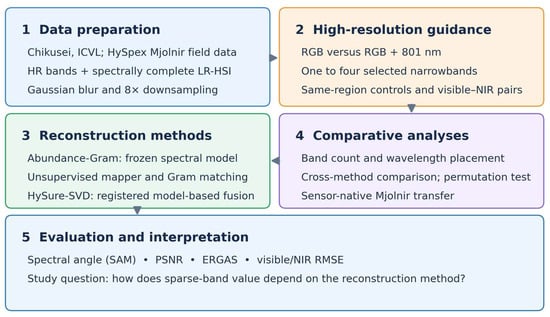
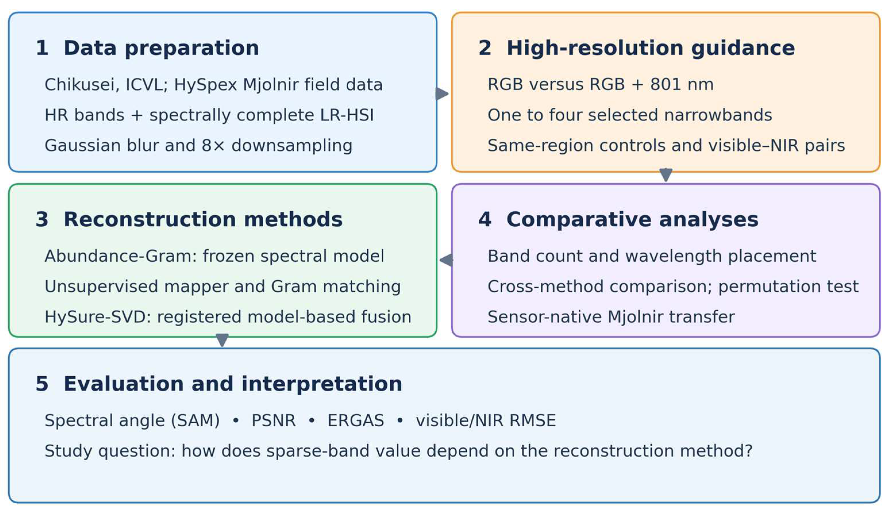
The overall study workflow is summarized in Figure 1. The same spectrally complete LR-HSI is paired with alternative high-resolution guide configurations; the resulting observations are reconstructed using abundance-Gram and HySure-SVD, followed by controlled spectral-placement comparisons, a permutation stress test, and evaluation on sensor-native Mjolnir channels.

Figure 1. Overview of the SparseHSR study workflow. Common hyperspectral data preparation and sparse high-resolution guide construction precede reconstruction using abundance-Gram and HySure-SVD. Existing analyses compare spectral-band number and placement, test guide permutation sensitivity, and evaluate sensor-native HySpex Mjolnir channels. SAM, PSNR, ERGAS, and regional RMSE are reported.

3.2. Correspondence-Free Abundance Representation

Let $A_L\in {\mathbb{R}}^{N_L\times K}$ and $A_H\in {\mathbb{R}}^{N_H\times K}$ denote the low- and high-resolution abundance representations produced by the same frozen spectral encoder, following standard hyperspectral unmixing concepts [22]. For an abundance matrix A, the normalized Gram matrix is

$$G\left(A\right)={\displaystyle \frac{1}{N}}{A}^{T}A$$

(3)

For any permutation matrix P, P^TP = I; therefore, the abundance-Gram statistic is invariant to pixel relabeling. This is the mechanism that removes the need for pixelwise correspondence between the low- and high-resolution abundance sets.

$$G\left(\mathit{PA}\right)={\displaystyle \frac{1}{N}}{A}^T{P}^T\mathit{PA}=G\left(A\right)$$

(4)

Because a permutation of image pixels changes only the row order of A, G(A) is unchanged. The training signal can therefore compare material-composition statistics between the LR-HSI and the high-resolution guide without requiring pixelwise spatial correspondence. Following the established implementation, the Gram matrix is also column-centered before the main discrepancy terms are computed, and its diagonal is matched separately to preserve abundance-energy structure.

3.3. High-Resolution Input-to-Spectrum Mapping

For reproducibility, the frozen spectral encoder contains three bias-free fully connected layers of dimensions 40 → 5, 45 → 5, and 50 → 40, each followed by ReLU; the second and third layers receive concatenated previous features. The spectral decoder is a bias-free 40 → 40 linear layer. The guide mapper is a bias-free n → 40 linear layer with a deterministic channel-repeat residual (n = 1–4). These specifications are from the unchanged source implementation; additional training-stage specifications are provided in Supplementary Table S2.

The LR-HSI is encoded directly by a dataset-specific pretrained 40-band encoder. For each dataset, this encoder/decoder decomposition is trained unsupervised from the corresponding spectrally complete LR-HSI before the sparse-guide experiments and is then frozen for all guide configurations; no HR-HSI reference is used to train the decomposition or the sparse-guide mapper. The high-resolution guide, containing one to four narrowbands or three-channel RGB, is zero-centered and passed through a residual linear mapper that expands it to 40 channels. The residual branch repeats each input channel to fill the 40-dimensional output (40 repeats for one band, 20 + 20 for two bands, 13 + 13 + 14 for three channels, and 10 repeats per channel for four channels), while a learned linear layer estimates a correction. The resulting pseudo-HSI is passed through the same frozen encoder, converted to a stick-breaking abundance representation, and decoded by a frozen 40-band linear decoder. The only optimized parameters are those of the high-resolution input-to-spectrum mapper. The number 40 is an experimental spectral grid rather than a requirement of the method: for a sensor with B native hyperspectral channels, the encoder, decoder, and mapper output can be defined directly on those B channels without resampling the spectrum to 1 nm intervals.

Let E and D denote the frozen encoder and decoder, R_rep the deterministic channel-repeat lift, and F_θ the learned linear correction. For sparse guide Y_G, the mapped pseudo-HSI and abundance representations are

X_M = R_rep(Y_G) + F_θ(Y_G)

(5)

A_L = E(Y_L),      A_H = E(X_M),      X_D = D(A_H)

(6)

3.4. Composite Abundance-Gram Objective

We retain the original composite loss used by the working reconstruction implementation. Let G_H and G_L denote the centered high- and low-resolution abundance Gram matrices, d_H and d_L their diagonals, and X_M and X_D the mapped pseudo-HSI and decoded HSI, respectively. The loss components are

$${ℒ}_{\mathrm{multi}}= L_{2,1}\left(G_H,G_L\right)+\mathrm{ERGAS}\left(G_H,G_L\right)+10\hspace{0.17em}\mathrm{SAM}\left(G_H,G_L\right)+\mathrm{SAM}\left(G_H^T,G_L^T\right)$$

(7)

$ℒ$_diag = L_2,1(d_H,d_L) + 10 SAM(d_H,d_L)

(8)

$ℒ$_rec = L_2,1(X_M,X_D)

(9)

$ℒ$ = 0.1 $ℒ$_rec + 10 $ℒ$_diag + 100 $ℒ$_multi

(10)

No HR-HSI reference enters this optimization objective. The reconstruction consistency term couples the mapped pseudo-HSI to the decoder output, while the remaining terms constrain abundance statistics to match those derived from the observed LR-HSI.

Observation-domain qualification. The loss in Equations (7)–(10) does not contain a separate hard constraint requiring a degraded HR prediction to reproduce the observed LR-HSI, nor an explicit data-fidelity term requiring the reconstructed HR bands to equal the guide at every pixel. The loss instead aligns global abundance statistics and the mapped/decoded spectra. Thus, the objective should not be interpreted as enforcing observation consistency in the sense used by classical model-based fusion; this difference is relevant to the comparison with HySure-SVD.

Loss-component ablations for this composite objective were already reported in our preceding TMM preprint [6]. Because SparseHSR adopts that objective unchanged and focuses on high-resolution spectral observation design, we do not repeat the loss ablation study in this manuscript.

3.5. Model Selection and Convergence

The best mapper checkpoint is selected by the minimum composite loss and is tested every epoch. Ground-truth reconstruction metrics are not used for checkpoint selection. Training termination is also unsupervised and uses two complementary criteria. First, the centered abundance Gram-SAM must decrease by at least 0.001 to reset a 5000-epoch patience counter. Second, because Gram statistics may continue to improve numerically after the reconstructed spectra have become visually and numerically stationary, the full predicted 40-band HSI is compared over non-overlapping 2000-epoch windows. The prediction is placed on an absolute scale using the observed LR-HSI spectral mean, and training stops when the relative L2 change is below 0.1% for two consecutive windows after epoch 5000. Thus, neither stopping criterion uses HR-HSI ground truth.

$${\theta }^{*}=\underset{\theta }{\arg \min }\hspace{0.33em}ℒ\left(\theta \right)$$

(11)

Here, θ denotes the trainable parameters, $ℒ$(θ) denotes the composite objective defined in Equations (7)–(10), and θ^* represents the parameter set with the minimum recorded objective value during checkpoint selection.

The second stopping criterion monitors the relative change of the reconstructed hyperspectral image over non-overlapping 2000-epoch windows.

$${\delta }_t={\displaystyle \frac{\parallel {\widehat{X}}_t-{\widehat{X}}_{t-2000}{\parallel }_2}{\parallel {\widehat{X}}_{t-2000}{\parallel }_2}}$$

(12)

Here, δ_t is the relative reconstruction change at epoch t; ${\widehat{X}}_t$ and ${\widehat{X}}_{t-2000}$ represent the reconstructed hyperspectral images at epochs t and t − 2000, respectively. The L₂ norm is computed over all pixels and spectral bands after radiometric recentering.

4. Datasets and Experimental Setup

4.1. Benchmark Datasets and Preprocessing

Chikusei is an airborne hyperspectral scene covering approximately 363–1018 nm [23]. A 1000 × 1000 spatial region is represented by 40 selected source bands, with representative anchors near 461, 549, 652, 714, 801, and 935 nm. ICVL provides natural-scene hyperspectral imagery [1]. The analyzed 40-band product spans 400–1000 nm; after applying the common spatial transform used by both the 40-band and visible products, an 800 × 800 crop is used. Its representative anchors are approximately 461, 549, 652, 708, 801, and 938 nm. The exact Chikusei and ICVL wavelength vectors are provided in Supplementary Table S3 and Table S4, respectively. The 16 predefined high-resolution guidance configurations and their dataset-specific nearest-band selection rules are documented in Supplementary Table S6 and the publicly available experiment code.

For both datasets, the LR-HSI is generated using Gaussian point-spread filtering (σ = 0.5) followed by spatial downsampling by a factor of eight. RGB guidance is synthesized from a separately prepared 31-band visible cube spanning 400–700 nm using the same fixed 3 × 31 B/G/R spectral response matrix for both datasets. The aligned 31-band visible cube and 40-band full-range cube are each normalized once by the same scalar, defined as the maximum pixel value across both products; no independent normalization is subsequently applied. For ICVL, both products undergo the same 90-degree rotation, horizontal mirroring, and 800 × 800 crop before normalization and RGB synthesis. The complete RGB spectral response coefficients are provided in Supplementary Table S5 and the publicly available experiment code.

Degradation and sensor-response scope. The Gaussian point-spread filter and eightfold downsampling establish a common controlled reduced-resolution setting rather than a measured modulation transfer function for a specific instrument. The fixed synthetic RGB response provides reproducible broadband guidance in the benchmark experiments but is not intended to represent a calibrated physical RGB camera. Consequently, the comparison isolates spectral-coverage effects under the specified forward model rather than establishing robustness across different sensor responses or degradation settings.

4.2. SparseHSR Study Design and Representative Spectral Sampling

The experiments follow the same causal sequence as the motivation. Stage 1 starts from the conventional RGB guide and adds one 801 nm high-resolution channel to test whether direct NIR guidance resolves the visible-only coverage gap. Stage 2 removes RGB and evaluates whether one to four sparse narrowbands alone can support full-spectrum reconstruction. Five single bands, same-region two-band controls, visible + NIR spanning pairs, anchored wavelength scans, and a predefined one-to-four-band progression separate channel count from spectral coverage. Together with RGB and RGB + 801, these form 16 high-resolution observation configurations per benchmark dataset. Stage 3 repeats the identical observation design with HySure-SVD to determine whether placement sensitivity belongs to the acquisition or to the reconstruction architecture. Stage 4 tests the registration mechanism by guide permutation and transfers the key sparse-band contrasts to sensor-native Mjolnir data.

4.3. Training and Evaluation Metrics

For the main abundance-Gram sweep, all 16 configurations use seed 0, Adam optimization with a learning rate of 1 × 10⁻⁴ and weight decay of 1 × 10⁻⁴, and a maximum of 1,000,001 epochs subject to the unsupervised stopping criteria described above. Reconstruction is evaluated every 200 epochs. To assess stochastic robustness without repeating the complete sweep, five representative configurations were additionally rerun with seeds 1 and 2: 801 nm alone, 461 + 549 nm, 801 + 935/938 nm, 549 + 801 nm, and 461 + 549 + 652 + 801 nm. These two additional runs were combined with the original seed-0 run to report three-seed mean and standard deviation of SAM. The same pretrained dataset-specific encoder/decoder, preprocessing, mapper architecture, optimizer, loss, checkpoint-selection criterion, and stopping rules were retained, so only mapper initialization/training stochasticity changed. We report spectral angle mapper (SAM), mean pixelwise spectral PSNR, ERGAS, and regional RMSE, with SAM treated as the primary metric because it directly measures spectral-shape agreement. PSNR is computed for each spatial pixel from the MSE of its reconstructed spectral vector using the global maximum squared reference intensity and is then averaged over pixels; this definition is stated explicitly because it differs from the alternative convention of averaging band-wise PSNR. Evaluation ERGAS uses the conventional spatial-resolution factor r = 8, i.e., the reported values include the 1/r factor. This reporting convention is separate from the fixed ERGAS-like discrepancy term inside the abundance-Gram training objective. Per-band RMSE is additionally summarized over the visible region (<=700 nm) and the NIR region (>700 nm). For abundance-Gram evaluation, the centered reconstruction is returned to the absolute radiometric frame by adding the 40-element per-band spectral mean measured from the observed LR-HSI. This observation-derived recentering uses only information available to the reconstruction system. HySure-SVD outputs its reconstruction directly in the observation model and does not use this recentering.

Radiometric comparison. The abundance-Gram output is recentered using the observed LR-HSI per-band mean because the mapper predicts centered spectra; HySure-SVD returns spectra in the original observation frame. These procedures are method-specific components of the original implementations, not a shared postprocessing transformation. All reported errors are computed after the respective outputs have been placed in the common normalized radiometric frame. The comparison is therefore between complete reconstruction procedures, including their objectives and reconstruction conventions, rather than an isolated architectural ablation.

Robustness scope. The targeted three-seed analysis is restricted to five selected configurations and does not provide a confidence interval for every result in the original seed-zero sweep. In particular, the RGB and RGB + 801 comparison is reported from the original sweep, and its percentage RMSE reductions should be interpreted as configuration-specific results rather than independently established multi-seed population effects.

4.4. HySure-SVD Baseline Protocol

After the SparseHSR abundance-Gram experiments established a strong dependence on sparse-guide spectral composition, HySure-SVD [7] was selected as a complete model-based comparison to determine whether that dependence was an acquisition property or an architecture property. HySure receives the same normalized LR-HSI, the same high-resolution guide, and the same scale-8 spatial degradation under all 16 configurations. For narrowband inputs, the spectral response is the exact n × 40 binary selection matrix. For RGB, because the guide is synthesized from the separately prepared 31-band visible product and therefore has no exact 40-band selection matrix, the 40-to-RGB response is estimated by nonnegative least squares using only the observed LR-HSI and a spatially degraded version of the observed HR-RGB; for RGB + 801, the exact 801 nm selection is appended to that observation-only RGB response. The spatial blur/downsampling operator is supplied exactly. The spectral subspace is estimated from the LR-HSI by SVD with p = 10. A single fixed parameter set is used for every dataset and configuration (p = 10, λφ = 5 × 10⁻⁴, λm = 1, and μ = 0.05), with no per-configuration tuning. The SALSA/ADMM solver runs in float64 for up to 20,000 iterations and is stopped only after four consecutive checks satisfy relative coefficient change <5 × 10⁻⁴, maximum primal residual <2 × 10⁻⁴, and relative objective change <1 × 10⁻⁴. No HR-HSI reference is used for fitting, parameter selection, or stopping; ground truth is used only for final metrics. All 32 HySure runs converged after 2375–6575 iterations.

To test registration dependence separately from spectral-placement accuracy, all 14 narrowband HySure configurations were also rerun after applying a fixed random permutation to the high-resolution guide pixels only, while leaving the LR-HSI and evaluation target in their original scene coordinates. This produced 28 permutation stress-test runs across the two datasets. The same spectral-selection matrices, spatial degradation model, SVD subspace dimension, and fixed HySure regularization parameters were used, with a 3000-iteration stress-test budget. The experiment is interpreted from the observation-domain optimization histories rather than from the terminal convergence flag alone: we examine whether the LR-HSI and guide residuals continue to decrease after permutation, together with the ADMM primal residual. HR-HSI ground truth is not used in fitting or in this registration test.

Permutation-test scope. Permuting guide pixels while retaining the original LR-HSI coordinate system is a deliberately extreme stress test of the correspondence assumptions, not a simulation of realistic geometric misregistration. Permutation invariance applies to the global Gram statistic: with a pixelwise guide mapper, the output spatial locations still follow the guide ordering unless the inverse permutation is applied. The test therefore illustrates a difference between training statistics and registered pixelwise fusion; it does not establish accurate spatial reconstruction under uncorrected alignment errors.

4.5. Sensor-Native Mjolnir Field Evaluation

After the benchmark patterns were established, a third dataset was used for a sensor-native field evaluation. The data originate from a published spring-wheat UAV study acquired at NIBIO with a HySpex Mjolnir V-1240 push-broom hyperspectral camera (Norsk Elektro Optikk AS, Oslo, Norway) [24]. The source instrument records 200 bands over approximately 400–1000 nm at about 3 nm sampling and 4 cm ground sampling distance. The public preprocessed data are associated with the Zenodo record reported in [24]. For the present experiment, a 1000 × 1000 field mosaic was represented by 40 sensor-native bands spanning 410.731–992.269 nm; no spectral interpolation was applied. The corresponding LR-HSI is the directly prepared 125 × 125 × 40 cube generated with the same scale-8 Gaussian degradation used in the benchmark study, and the HR and LR products retain a single shared normalization. Importantly, the field experiment was used to test transfer of the already observed benchmark contrasts rather than to re-optimize wavelength locations or method parameters.

Field-validation scope. Although the spectral channels are native measurements of an airborne HySpex instrument, the LR-HSI and HR guidance used for reconstruction are derived from the same field mosaic. This constitutes sensor-native spectral sampling with simulated spatial degradation, not a validation using independently acquired and registered sensors at two spatial resolutions.

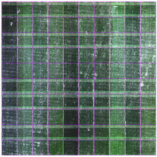
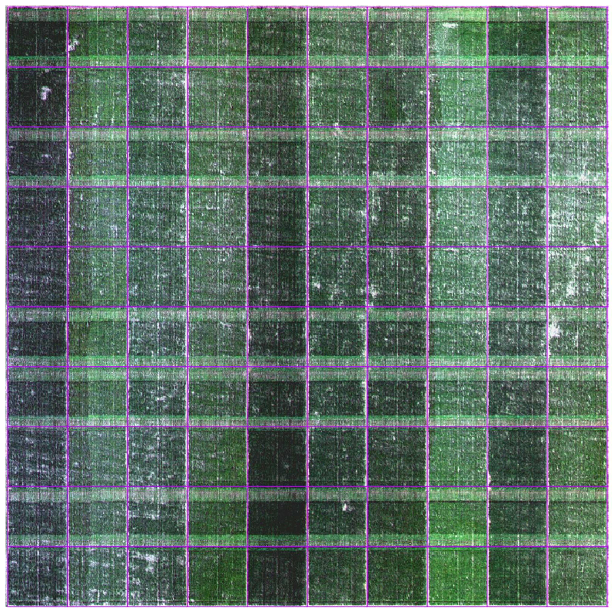
The actual Mjolnir channels nearest the nominal anchors are 460.410, 548.079, 653.282, 802.320, and 933.823 nm. Seven focused narrowband configurations were evaluated: 802 alone; 460 + 548; 802 + 934; 548 + 802; 653 + 802; 460 + 548 + 802; and 460 + 548 + 653 + 802 nm. RGB-related inputs were intentionally omitted because this field evaluation is designed to test transfer of the narrowband placement and band-count findings using sensor-native channels. For the abundance-Gram method, the encoder/decoder decomposition was trained unsupervised on the Mjolnir LR-HSI and frozen before guide mapping; the same composite objective and unsupervised stopping rules were then used. HySure estimates its p = 10 SVD subspace from the same LR-HSI and retains the identical fixed regularization and convergence settings used for Chikusei and ICVL. The field HR-HSI is used only for post hoc evaluation. Metrics are reported over the full valid field mosaic and, separately, over the agricultural plot mask. Figure 2 provides an overview of the prepared 40-band Mjolnir field mosaic used for this field evaluation, shown as an RGB composite using the nearest native bands to 653, 548, and 460 nm; purple outlines indicate the extracted plot boundaries used for plot-level masking.

Figure 2. Overview of the airborne HySpex Mjolnir field dataset used for field evaluation. The prepared hyperspectral mosaic covers 100 × 100 m at 4 cm ground sampling distance and contains 40 selected native bands spanning 410.7–992.3 nm. The displayed image is an RGB composite generated from the native bands nearest 653, 548, and 460 nm. Purple outlines indicate the 10 × 10 m spaced plot grid used to derive the plot mask for masked evaluation. In some rows, plot borders were harvested, which led to visible pathways with less vegetation cover. The differences in canopy vigor are due to different fertilization strategies in early spring. Some of the plots do not show complete canopy closure, thus presenting areas of bare soil.

5. Results

5.1. Extending RGB Guidance into the Near-Infrared Recovers Missing High-Resolution Information

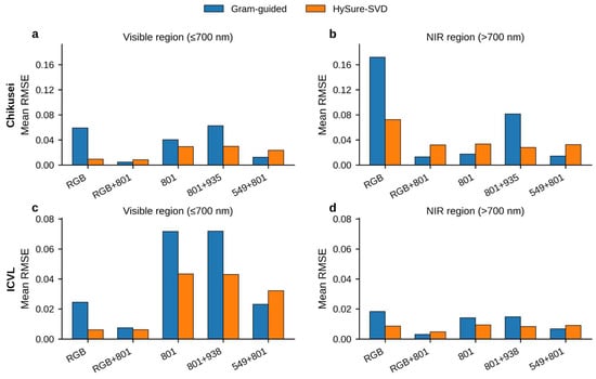
SparseHSR starts where practice starts: an RGB guide. RGB observes the visible range directly but never measures the NIR, so once the target spectrum extends past the visible boundary the reconstruction must fill that region with no direct high-resolution constraint. On Chikusei the consequence is stark—RGB-only mean per-band RMSE is 0.0592 in the visible but 0.1718 in the NIR. ICVL shows a milder version of the same gap: its RGB-only NIR error is lower, yet the NIR is still reconstructed without any direct high-resolution NIR observation.

Adding a single direct high-resolution NIR observation at 801 nm substantially reduces the error associated with the missing direct NIR constraint. On Chikusei, the visible and NIR RMSE fall to 0.00478 and 0.01321 and the full-spectrum mean to 0.00878, a 92.2% reduction; on ICVL, the full-spectrum mean drops from 0.02143 to 0.00524, a 75.5% reduction. These quantitative results are summarized in Table 1, while the regional RMSE comparisons between abundance-Gram and HySure-SVD are illustrated in Figure 3. These reductions are obtained with the abundance-Gram reconstruction. The gain is consistent across two very different scenes, showing that extending high-resolution guidance beyond RGB can recover information visible-only guidance cannot directly supply. It also sets up the rest of the paper: if one NIR band produces this much improvement, the high-resolution sensor can perhaps be rebuilt around a handful of well-chosen spectral measurements.

Table 1. Abundance-Gram mean per-band RMSE for the motivating RGB/near-infrared comparison and key narrowband configurations.

Input	Chik. Vis	Chik. NIR	Chik. Full	ICVL Vis	ICVL NIR	ICVL Full
RGB	0.0592	0.1718	0.1127	0.0245	0.0183	0.0214
RGB + 801	0.0048	0.0132	0.0088	0.0074	0.0031	0.0052
801	0.0406	0.0174	0.0296	0.0716	0.0142	0.0429
801 + 935	0.0628	0.0815	0.0717	0.0719	0.0148	0.0433
549 + 801	0.0125	0.0142	0.0133	0.0231	0.0067	0.0149

Figure 3. Comparison of mean per-band RMSE between abundance-Gram and HySure-SVD for representative high-resolution guidance configurations. (a) Chikusei, visible region (≤700 nm); (b) Chikusei, near-infrared region (>700 nm); (c) ICVL, visible region (≤700 nm); and (d) ICVL, near-infrared region (>700 nm). Blue and orange bars represent abundance-Gram and HySure-SVD, respectively. Lower RMSE indicates better reconstruction accuracy.

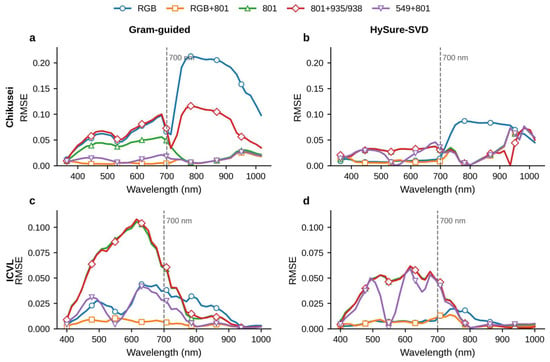
The wavelength-resolved profiles tell the same story (Figure 4): on Chikusei, RGB-only error climbs sharply past the visible-NIR boundary while RGB + 801 suppresses it across most of the NIR, and on ICVL the lower baseline error still improves with the added 801 nm anchor. The two scenes differ in how badly the missing NIR observation hurts, not in whether RGB ever measures the NIR—it does not. This is the hinge of the study: if a single added band recovers most of what RGB cannot see, the obvious next question is whether the three broadband RGB channels are themselves necessary, or whether a few narrowbands can do the same job with far less high-resolution data. The remaining experiments pursue exactly that.

Figure 4. Wavelength-dependent reconstruction RMSE for representative high-resolution guidance configurations. (a) Chikusei reconstructed using abundance-Gram; (b) Chikusei reconstructed using HySure-SVD; (c) ICVL reconstructed using abundance-Gram; and (d) ICVL reconstructed using HySure-SVD. Colored curves correspond to the five guidance configurations indicated in the legend. The vertical dashed line marks the 700 nm boundary between visible and near-infrared wavelengths.

5.2. Narrowband-Only Guidance Is Viable, but Single-Band Preference Varies Between Datasets

We begin dismantling the RGB assumption at the extreme: a guide of one high-resolution narrowband. This is deliberately underconstrained—one spatially detailed spectral measurement, with the full spectral basis still coming from the low-resolution HSI. In the main seed-0 sweep, reconstruction stays functional, but no single wavelength wins everywhere. On Chikusei the lowest single-band seed-0 SAM is obtained at 801 nm (6.12°), followed by 935 nm (7.10°), with the visible single bands at 8.99° to 10.17°. On ICVL the order inverts: 549 nm is best (2.67°), just ahead of 652 nm (2.71°), while 801 and 938 nm are weaker at 3.63° and 4.30°. The complete single-band reconstruction metrics for both datasets are reported in Table 2. The later multi-seed analysis shows that the isolated 801 nm case is substantially seed-sensitive on Chikusei, reinforcing the conclusion that a lone narrowband is an underconstrained design rather than a universally reliable optimum.

Table 2. Representative single-band reconstruction results.

Chikusei nm	SAM	PSNR	ERGAS (r = 8)	ICVL nm	SAM	PSNR	ERGAS (r = 8)
461	8.990	24.35	5.81	461	3.094	36.40	1.24
549	10.171	25.03	6.69	549	2.668	36.78	1.16
652	10.037	24.85	6.98	652	2.709	36.83	1.16
801	6.119	34.04	6.72	801	3.625	31.95	1.78
935	7.097	32.84	6.99	938	4.302	29.24	2.37

5.3. A Second Band Matters Most When It Adds Complementary Spectral Coverage

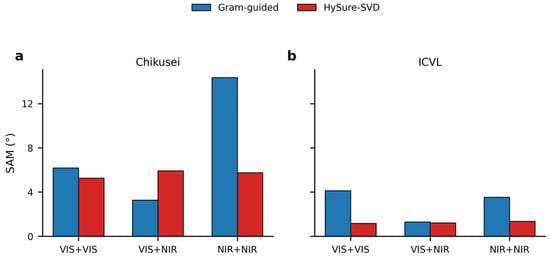
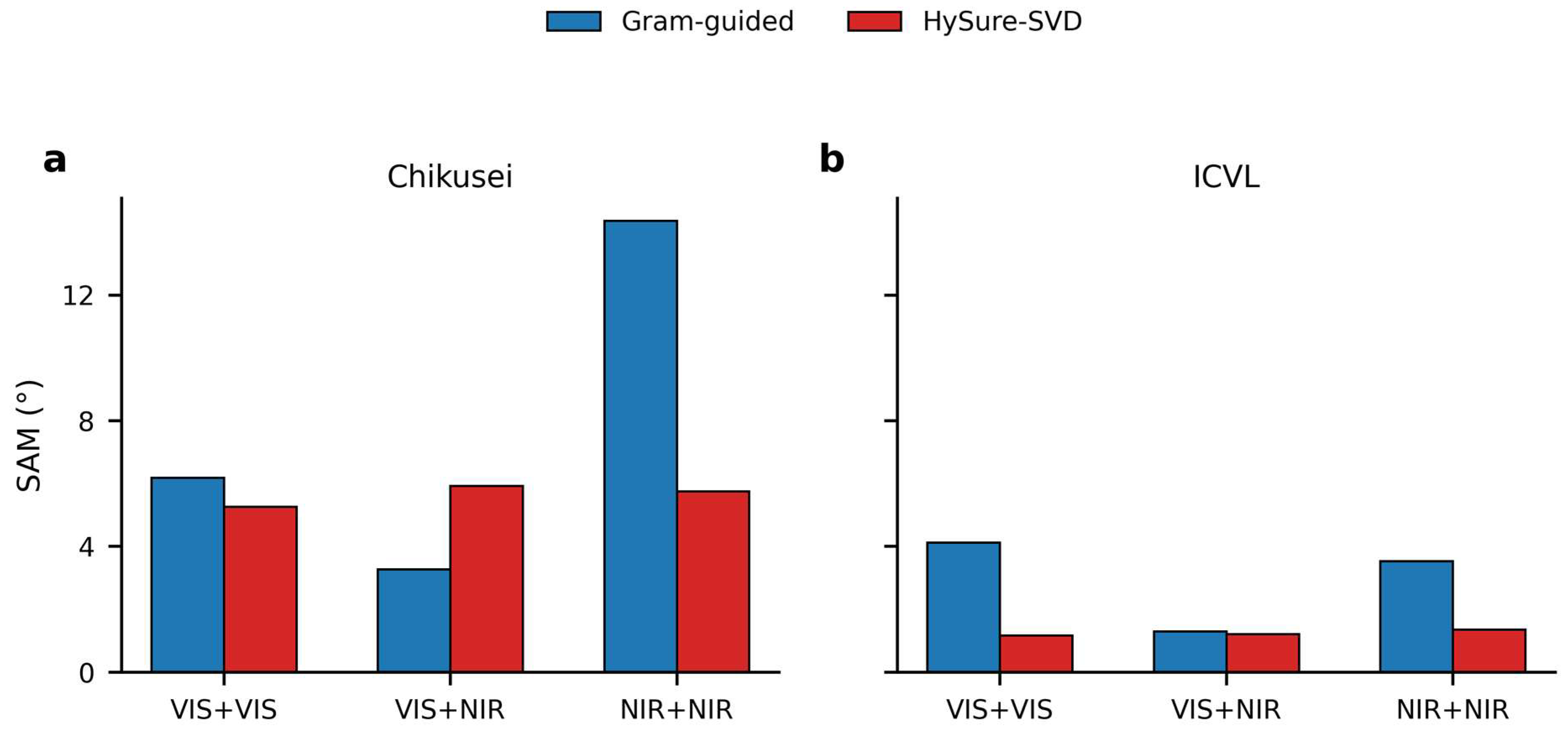
A second band shifts the question from coverage to placement: given two high-resolution measurements, does it matter where the second one sits? In the main seed-0 sweep, equal-count two-band controls answer cleanly. On Chikusei, the five visible + NIR pairs average an abundance-Gram SAM of 3.66°, against 6.18° for the visible + visible control (461 + 549) and 14.36° for the NIR + NIR control (801 + 935); the matching ICVL means are 1.68°, 4.12°, and 3.53°. Relative to the same-region controls, spanning the visible and NIR cuts SAM by 40.7% versus visible + visible and 74.5% versus NIR + NIR on Chikusei, and by 59.2% and 52.4% on ICVL. Every configuration uses exactly two high-resolution bands, so the improvement comes from spectral complementarity, not from more channels. The targeted multi-seed test in Section 5.9 confirms the stability of the 549 + 801 spanning pair on both datasets, while showing that the ICVL visible-only control is more seed-sensitive. The comparison between same-region and spectrally complementary two-band configurations for both reconstruction methods is illustrated in Figure 5.

Figure 5. Reconstruction spectral angle mapper (SAM, degrees) for three equal-count two-band configurations using abundance-Gram and HySure-SVD. (a) Chikusei dataset; (b) ICVL dataset. The configurations represent visible + visible (461 + 549 nm), visible + NIR (549 + 801 nm), and NIR + NIR (801 + 935/938 nm) guidance. Blue bars indicate abundance-Gram and red bars indicate HySure-SVD. Lower SAM indicates better spectral reconstruction.

Among the tested pairs, 652 + 801 nm gives the lowest abundance-Gram SAM on both datasets (3.26° on Chikusei, 1.20° on ICVL). The predefined 549 + 801 pair is essentially tied on Chikusei and remains highly competitive on ICVL, where it gives slightly lower ERGAS. The corresponding two-band reconstruction metrics are presented in Table 3. We therefore keep 549 + 801 as a balanced reference pair and do not read 652 + 801 as a globally optimal combination. The lesson is regional rather than pinpoint: a visible anchor paired with a well-separated NIR anchor is what matters.

Table 3. Representative two-band reconstruction results.

Chik. Pair	Region	SAM	PSNR	ERGAS (r = 8)	ICVL Pair	SAM	PSNR	ERGAS (r = 8)
461 + 549	Vis + Vis	6.175	29.66	3.91	461 + 549	4.124	34.66	1.47
801 + 935	NIR + NIR	14.356	25.58	10.47	801 + 938	3.534	31.97	1.79
461 + 801	Vis + NIR	3.364	38.92	2.60	461 + 801	2.266	40.71	1.10
549 + 801	Vis + NIR	3.273	39.13	2.75	549 + 801	1.289	46.65	0.64
652 + 801	Vis + NIR	3.259	39.79	2.99	652 + 801	1.199	46.31	0.65
549 + 714	Vis + NIR	4.664	36.28	3.17	549 + 708	2.089	41.47	0.98
549 + 935	Vis + NIR	3.745	37.63	2.89	549 + 938	1.575	41.78	0.74

5.4. Controlled Anchor Scans Localize the Most Useful Tested Regions

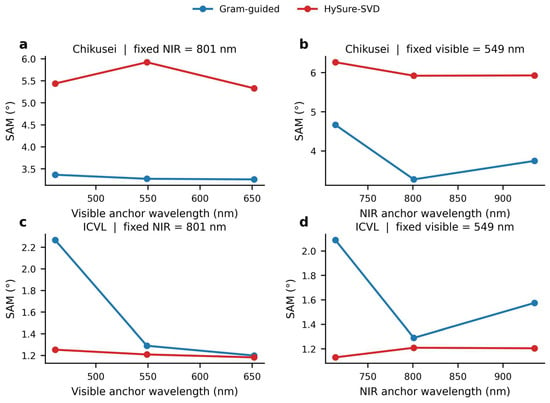
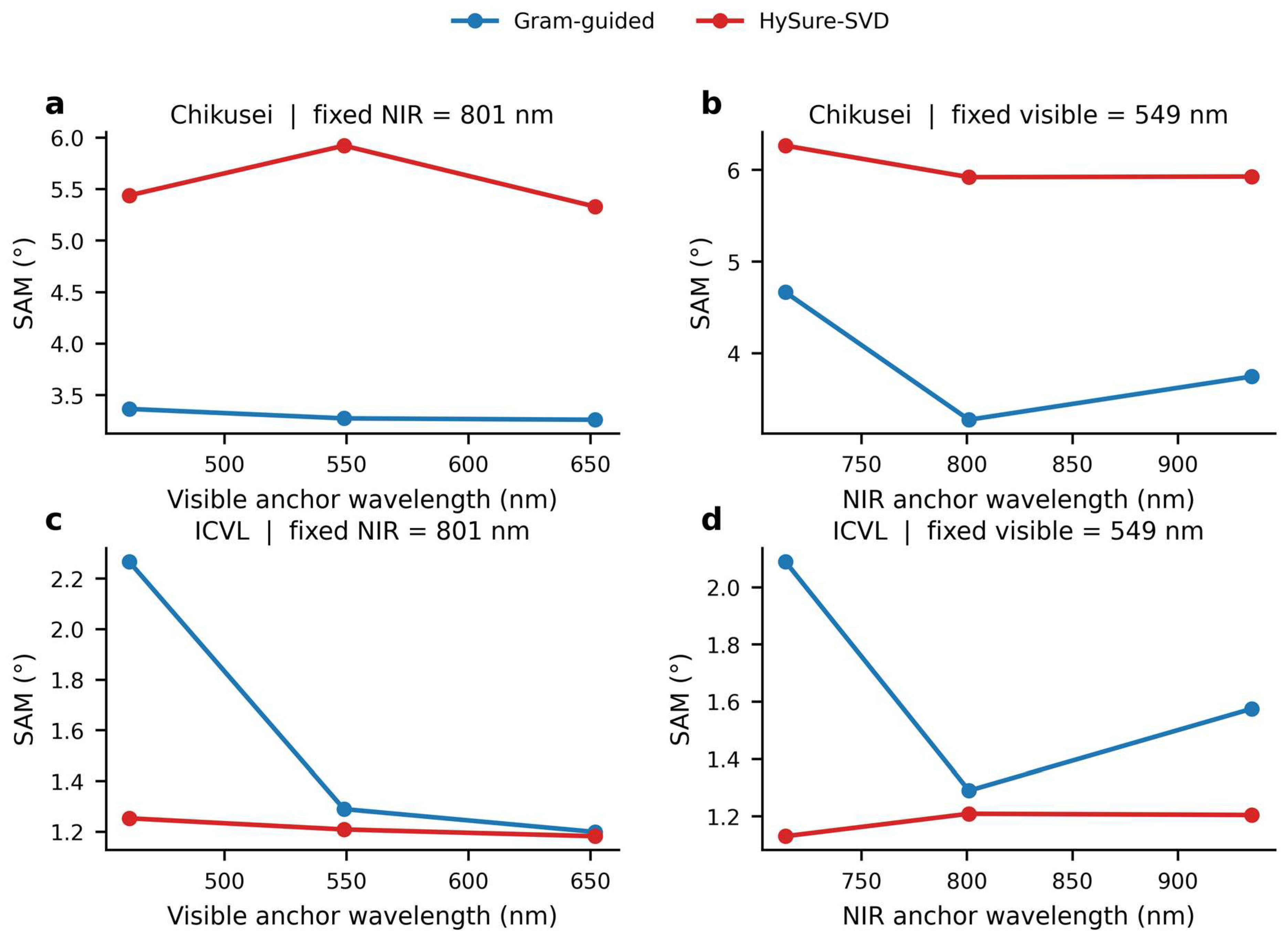
Complementarity says separation helps, but not which regions. Fixing the NIR anchor near 801 nm and sliding the visible band from 461 to 549 to 652 nm improves abundance-Gram SAM on both datasets—modestly on Chikusei (3.36°, 3.27°, 3.26°) and strongly on ICVL (2.27°, 1.29°, 1.20°). Fixing the visible anchor near 549 nm instead, 801 nm is the best tested NIR partner on both scenes: Chikusei gives 4.66° at 714 nm, 3.27° at 801 nm, and 3.74° at 935 nm, and ICVL gives 2.09° at 708 nm, 1.29° at 801 nm, and 1.57° at 938 nm. A mid-to-long visible anchor paired with an approximately 800 nm NIR measurement is thus an efficient region pair in these scenes, without claiming an exact universal optimum. The wavelength-dependent reconstruction performance for both datasets and reconstruction methods is illustrated in Figure 6.

Figure 6. Controlled wavelength-location scans comparing abundance-Gram and HySure-SVD reconstruction accuracy. (a) Chikusei: varying the visible-band wavelength while fixing the NIR anchor at approximately 801 nm; (b) Chikusei: varying the NIR-band wavelength while fixing the visible anchor at approximately 549 nm; (c) ICVL: varying the visible-band wavelength while fixing the NIR anchor at approximately 801 nm; and (d) ICVL: varying the NIR-band wavelength while fixing the visible anchor at approximately 549 nm. Blue and red curves represent abundance-Gram and HySure-SVD, respectively. Performance is measured using SAM (degrees), with lower values indicating better reconstruction.

5.5. Distributed Coverage Captures the Largest Early Gain from One to Four Narrowbands

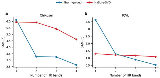
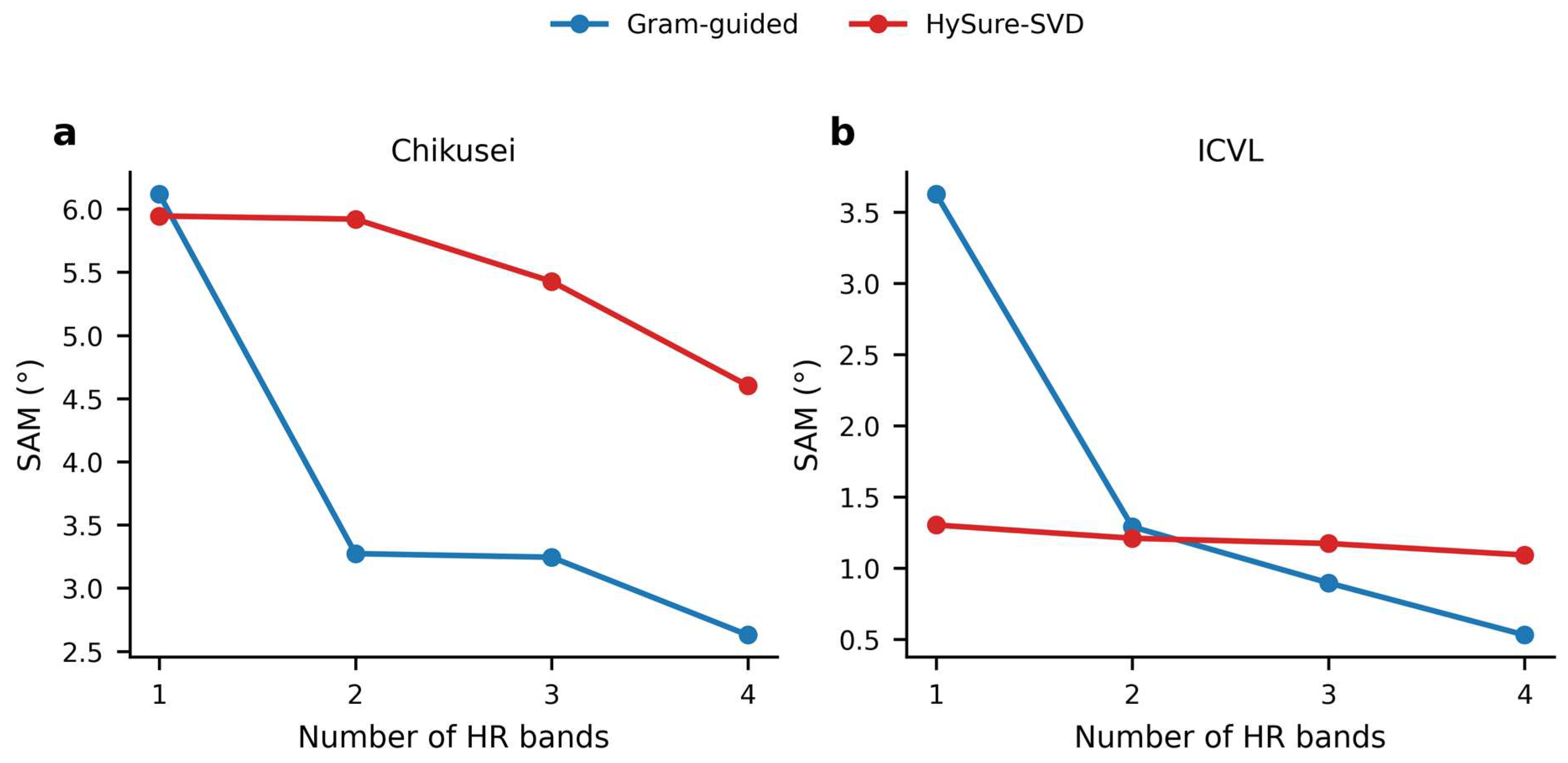
Having seen that single-band preference varies between datasets and that two well-separated bands are much stronger, we ask how quality scales as coverage is enriched. In the main seed-0 sweep, along the predefined path 801 → 549 + 801 → 461 + 549 + 801 → 461 + 549 + 652 + 801 nm, the biggest single jump comes first, when the initial complementary visible band joins the 801 nm input: Chikusei improves from 6.12° to 3.27° SAM (46.5%) and ICVL from 3.63° to 1.29° (64.4%). Further bands still help, but with dataset-dependent, diminishing returns—on Chikusei the third band barely moves SAM (3.27° to 3.24°) before the fourth reaches 2.63°, whereas on ICVL the third and fourth push down to 0.90° and 0.53°. The targeted three-seed repeats confirm that both the 549 + 801 pair and the four-band endpoint are highly stable, so the central gain from distributed coverage is not a seed-0 accident. Detailed SAM, PSNR, and ERGAS values for the one-to-four-band progression are provided in Table 4. The corresponding reconstruction performance across the one-to-four-band progression is illustrated in Figure 7.

Table 4. Progressive one-to-four-band spanning sequence.

Bands	Configuration	Chikusei SAM	PSNR	ERGAS (r = 8)	ICVL SAM	PSNR	ERGAS (r = 8)
1	801	6.119	34.04	6.72	3.625	31.95	1.78
2	549 + 801	3.273	39.13	2.75	1.289	46.65	0.64
3	461 + 549 + 801	3.244	39.31	2.21	0.896	48.63	0.49
4	461 + 549 + 652 + 801	2.629	40.94	1.81	0.530	51.30	0.18

Figure 7. Effect of increasing the number of distributed high-resolution narrowbands on reconstruction SAM. (a) Chikusei dataset; (b) ICVL dataset. The one-, two-, three-, and four-band configurations correspond to 801 nm, 549 + 801 nm, 461 + 549 + 801 nm, and 461 + 549 + 652 + 801 nm, respectively. Blue and red curves represent abundance-Gram and HySure-SVD. Lower SAM indicates better reconstruction accuracy.

Four distributed narrowbands nearly match broadband RGB plus an NIR channel. On Chikusei the four-band guide reaches SAM 2.63°, mean pixelwise spectral PSNR 40.94 dB, and scale-normalized ERGAS 1.81, against 2.47°, 41.32 dB, and 1.77 for RGB + 801. This closes the loop opened by the motivating experiment: the value of adding 801 nm to RGB was complementary coverage, not RGB itself or NIR dominance. In the tested fusion setting, a compact, strategically placed narrowband set can stand in for three broadband visible channels plus an explicit NIR band, reducing the amount of high-resolution spectral information that must be acquired.

5.6. HySure Comparison Reveals Architecture-Dependent Placement Sensitivity

So far, the complete 16-configuration abundance-Gram sweep has been reported from seed 0. This raises a broader question: within the present comparison, is placement sensitivity driven mainly by the measurements or by the reconstruction mechanism that consumes them? To test this, we ran HySure-SVD [7] on the same 16 high-resolution configurations for both benchmark datasets. All 32 runs converged under the fully unsupervised protocol of Section 4.4. Sparse high-resolution observations help both methods; what differs sharply is how much their spectral placement matters. Representative abundance-Gram and HySure-SVD results under identical narrowband configurations are compared in Table 5. Section 5.9 separately tests abundance-Gram seed robustness for five representative configurations.

Table 5. Representative cross-method narrowband reconstruction SAM (degrees). HySure was evaluated on all 16 configurations; abundance-Gram entries are from the main seed-0 sweep, with targeted three-seed robustness reported separately in in Section 5.9.

Configuration	Gram Chik.	HySure Chik.	Gram ICVL	HySure ICVL
801 (single)	6.119	5.945	3.625	1.302
Vis + Vis 461 + 549	6.175	5.262	4.124	1.162
NIR + NIR 801 + 935	14.356	5.751	3.534	1.345
Spanning 549 + 801	3.273	5.920	1.289	1.209
Spanning 652 + 801	3.259	5.328	1.199	1.182
4 spanning bands	2.629	4.603	0.530	1.091

The contrast is large. Across the narrowband configurations, abundance-Gram spans 2.63–14.36° SAM on Chikusei (5.46×) and 0.53–4.30° on ICVL (8.12×), while HySure spans only 4.60–6.26° (1.36×) and 1.09–1.34° (1.23×). In the controlled two-band comparison HySure returns 5.262°, 5.751°, and 5.920° on Chikusei for 461 + 549, 801 + 935, and 549 + 801, and 1.162°, 1.345°, and 1.209° on ICVL—so the visible + NIR pair is not consistently HySure’s best input, the opposite of the strong same-region penalty seen in abundance-Gram.

HySure still uses extra guidance well. Along the same one-to-four-band sequence its SAM improves from 5.945° to 4.603° on Chikusei and from 1.302° to 1.091° on ICVL, while abundance-Gram improves from 6.119° to 2.629° and from 3.625° to 0.530°. The ranking is genuinely two-sided: HySure is stronger for several isolated or spectrally clustered guides, whereas abundance-Gram gains far more from distributed inputs and overtakes once both visible and NIR constraints are present. On ICVL, HySure even edges abundance-Gram for 549 + 801 (1.209° versus 1.289°). The result is therefore not that one method wins, but that these two architectures convert sparse guidance into reconstruction value differently.

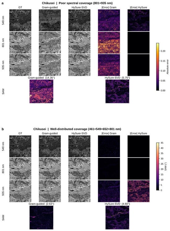
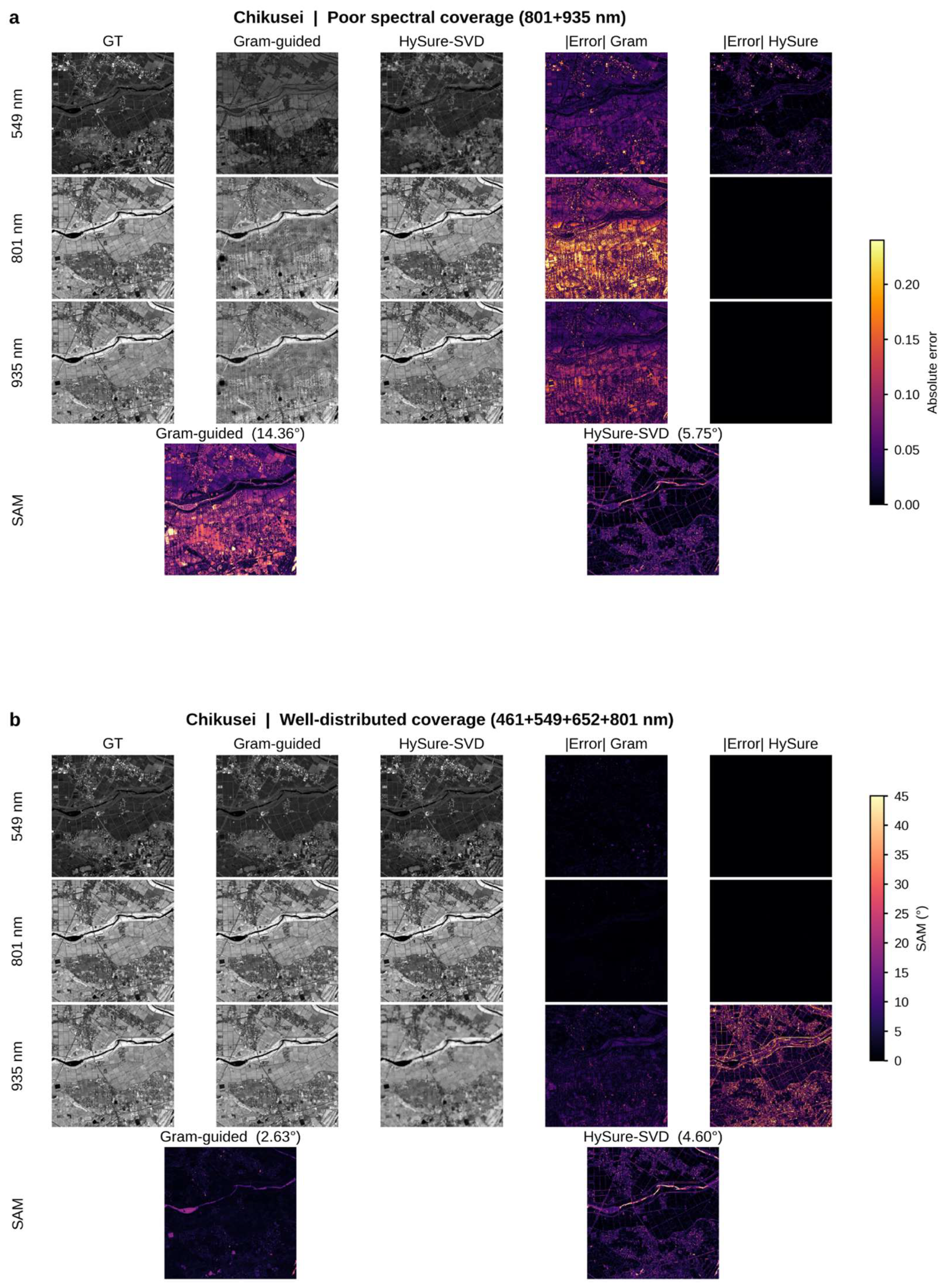
Figure 8 makes the crossover spatial on Chikusei. With the clustered 801 + 935 nm guide, HySure holds far lower mean SAM than abundance-Gram (5.75° versus 14.36°) and nearly zeroes error at the directly observed channels. With four distributed bands (461 + 549 + 652 + 801 nm), the order flips—mean SAM falls to 2.63° for abundance-Gram while HySure stays at 4.60°—and the unmeasured 935 nm band is also cleaner for abundance-Gram, showing that distributed guidance improves the whole spectrum, not only the measured wavelengths.

Figure 8. Qualitative comparison of hyperspectral reconstruction on Chikusei under two high-resolution guidance configurations. (a) Spectrally clustered two-band guidance using 801 + 935 nm; (b) distributed four-band guidance using 461 + 549 + 652 + 801 nm. Within each panel, the first three rows show the 549, 801, and 935 nm spectral bands, respectively. Columns display the ground truth (GT), abundance-Gram reconstruction, HySure-SVD reconstruction, and their corresponding absolute-error maps. The bottom row presents pixelwise spectral angle mapper (SAM) maps for abundance-Gram and HySure-SVD, with mean SAM values indicated above each map. Lower absolute error and SAM indicate better reconstruction accuracy.

5.7. Sensor-Native Mjolnir Data Reproduce the Benchmark Crossover

Three findings now stand on the benchmarks: RGB provides no direct high-resolution NIR observation, although the magnitude of the resulting reconstruction penalty differs between datasets; a few sparse visible–NIR bands can replace RGB because the low-resolution HSI stays spectrally complete; and the two tested reconstruction architectures value a given placement differently. The remaining question is whether these patterns survive outside idealized benchmark-band extraction. We therefore repeat the key configurations using native channels from HySpex Mjolnir airborne imagery.

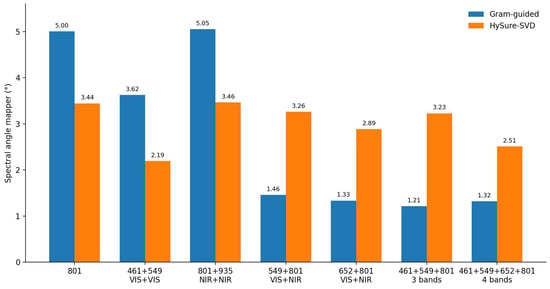
The abundance-Gram pattern transfers directly. A single 802.320 nm guide gives full-field SAM 5.002°, and same-region two-band controls stay weak (3.625° for 460.410 + 548.079 nm, 5.053° for 802.320 + 933.823 nm). Spanning pairs are far stronger: 548.079 + 802.320 and 653.282 + 802.320 nm reach 1.455° and 1.335°. A third distributed band lowers SAM to 1.212°, while the four-band guide gives 1.318° SAM but the lowest scale-normalized ERGAS (0.593 versus 0.610 for three bands)—again diminishing, metric-dependent returns rather than a simple more-is-better rule.

HySure shows the complementary behavior. Its Mjolnir SAM is 3.442° for 802 nm alone, 2.192° for the visible-only 460 + 548 pair, 3.463° for 802 + 934, 3.259° for 548 + 802, and 2.886° for 653 + 802, with the three- and four-band inputs at 3.227° and 2.509°. HySure thus beats abundance-Gram for the isolated and same-region inputs and loses when guidance is well distributed across visible and NIR—the benchmark crossover persists in this sensor-native-band evaluation. All seven HySure field runs met the unsupervised convergence criterion after 3775–4650 iterations, and plot-mask SAM differs from full-field SAM by under 0.03°, so background pixels are not driving the effect. The full-field SAM values for all seven sensor-native guidance configurations are summarized in Table 6. Because the sparse guide channels and LR-HSI are derived from the same Mjolnir hyperspectral product, this experiment validates transfer across native sensor channels and scene content, not a physically separate multisensor hardware system. Figure 9 summarizes the field crossover. The same qualitative division seen on Chikusei and ICVL remains: HySure-SVD is stronger for isolated or spectrally clustered guidance, whereas abundance-Gram improves sharply once high-resolution observations span visible and NIR regions.

Table 6. Mjolnir full-field reconstruction SAM (degrees) for the focused sensor-native narrowband evaluation.

Configuration	Gram SAM	HySure SAM
802 (single)	5.002	3.442
Vis + Vis 460 + 548	3.625	2.192
NIR + NIR 802 + 934	5.053	3.463
Spanning 548 + 802	1.455	3.259
Spanning 653 + 802	1.335	2.886
460 + 548 + 802	1.212	3.227
460 + 548 + 653 + 802	1.318	2.509

Figure 9. Sensor-native Mjolnir field evaluation. Full-field spectral angle mapper (SAM) for abundance-Gram and HySure-SVD under seven sparse narrowband configurations. Labels use nominal anchor wavelengths; the nearest native Mjolnir channels are 460.410, 548.079, 653.282, 802.320, and 933.823 nm. The benchmark crossover persists: HySure is comparatively strong for isolated or clustered guides, while abundance-Gram becomes markedly stronger with distributed visible + NIR coverage.

5.8. Permutation Stress Test Explains the Complementary Cost of HySure

The field and benchmark results establish that HySure is less sensitive to sparse-guide wavelength placement. The complementary question is what that robustness costs. Our objective matches the abundance Gram matrix between resolutions, a second-order statistic invariant to pixel relabeling: for an abundance matrix A and any permutation P, (PA)^T(PA) = A^TP^TPA = A^TA. The optimization statistic therefore does not depend on pixel-to-pixel correspondence between the low- and high-resolution abundance sets.

HySure, by contrast, uses an explicit registered observation model. When only the high-resolution guide was randomly permuted, the optimizer rapidly reached a persistent data-fidelity plateau. Across the 28 narrowband permutation runs, the final relative guide residual ranged from 0.92% to 11.65% (median 2.86%), compared with 0.16% to 1.25% (median 0.29%) for the corresponding registered runs. In 27 of 28 permutation runs, the guide residual at iteration 100 was already within 1% of its value at iteration 3000, and all 28 were within 5%; the median first iteration within 1% of the terminal guide residual was 75. At iteration 3000, the ADMM maximum primal residual was already small (median 5.5 × 10⁻⁶; maximum 1.27 × 10⁻⁴), although the latent coefficient field continued to drift enough that none of the 28 runs satisfied the joint stopping rule. All 28 corresponding registered narrowband runs converged. The failure is therefore structural rather than an early-cutoff artifact: permutation makes the two observations incompatible under HySure’s registered forward model, whereas the abundance-Gram statistic is unchanged.

5.9. Targeted Multi-Seed Analysis Confirms Robustness of the Key Spanning Designs

To test whether the principal abundance-Gram findings depend on mapper initialization, we repeated five representative configurations with seeds 1 and 2 and combined them with the original seed-0 runs. The two key distributed designs are highly reproducible on both datasets. For 549 + 801 nm, SAM is 3.27279 ± 0.00004° on Chikusei and 1.28972 ± 0.00038° on ICVL. For the four-band 461 + 549 + 652 + 801 nm guide, SAM is 2.61426 ± 0.01721° and 0.53523 ± 0.00456°, respectively. These configurations retain the same ordering in every seed: the four-band spanning design ranks first and 549 + 801 ranks second on both datasets. The three-seed mean SAM and sample standard deviation for each representative configuration are reported in Table 7.

Table 7. Three-seed abundance-Gram robustness for five representative configurations. Values are mean and sample standard deviation (n − 1) of reconstruction SAM over seeds 0, 1, and 2.

Dataset	Configuration (nm)	SAM Mean (deg)	SAM SD (deg)
Chikusei	801	11.314108	6.601227
Chikusei	461 + 549	6.174651	0.003320
Chikusei	801 + 935	14.363969	0.035533
Chikusei	549 + 801	3.272785	0.000042
Chikusei	461 + 549 + 652 + 801	2.614263	0.017210
ICVL	801	3.638991	0.040483
ICVL	461 + 549	3.252400	1.542681
ICVL	801 + 938	3.598431	0.110294
ICVL	549 + 801	1.289719	0.000380
ICVL	461 + 549 + 652 + 801	0.535234	0.004558

The additional seeds also reveal where optimization sensitivity remains. The single 801 nm guide on Chikusei varies widely (11.314 ± 6.601°; individual seeds 6.119°, 9.081°, and 18.742°), and the 461 + 549 nm visible-only control on ICVL is likewise variable (3.252 ± 1.543°) because seed 1 reaches 1.471° while seeds 0 and 2 remain near 4.1°. By contrast, the same-region controls are otherwise stable or moderately variable, and neither instability changes the central ordering of the distributed designs. The robustness experiment therefore sharpens the interpretation: the main evidence for sparse visible-NIR sensing comes from the stable spanning configurations, whereas isolated or spectrally clustered guides can be both less accurate and more optimization-sensitive.

6. Discussion

6.1. From Visible-Range RGB Guidance to Sparse Visible–NIR Sensing

SparseHSR grows from one limitation of RGB-guided, visible-range reconstruction: RGB never observes the NIR directly, and that only bites once the target spectrum extends beyond the visible. The spectrally complete low-resolution HSI still supplies the full spectral basis, but fine NIR structure must be inferred with no direct high-resolution NIR constraint. Adding one 801 nm channel supplies exactly that missing observation and produces large full-spectrum error reductions on both benchmarks.

That single result reframes the practical question from how RGB can recover the NIR to how little high-resolution spectral information is actually required. The one-to-four-band experiments answer that the guide can shrink to a few well-placed visible-NIR measurements while the low-resolution HSI holds the complete prior. The engineering takeaway is therefore not a magic wavelength but a real reduction in high-resolution spectral measurement burden relative to dense hyperspectral acquisition.

6.2. What Generalizes Across Architectures, and What Does Not

Two things separate cleanly across the two tested architectures: what generalizes within this comparison—a spectrally complete low-resolution HSI plus very sparse high-resolution bands can support full visible–NIR reconstruction for both methods—and what does not—how much performance depends on where those bands sit. Abundance-Gram is heavily penalized by clustered guides and rewarded by distributed visible-NIR coverage, whereas HySure-SVD is much flatter and can even prefer same-region bands. The targeted three-seed analysis strengthens the abundance-Gram side of this comparison by showing that the 549 + 801 and four-band spanning designs are exceptionally stable across initialization, while some weaker isolated or same-region configurations are more seed-sensitive. Sparse acquisition is viable for both tested methods, but sparse-band value is neither architecture-independent nor equally robust across all guide designs.

Architecture dependence is therefore a result of the controlled two-method comparison, not the premise of the study. HySure-SVD uses registered pixelwise observations and stays effective with clustered guides as long as registration holds. Abundance-Gram drops the correspondence requirement by matching global second-order statistics, which makes informative spectral coverage matter more. The permutation stress test makes this mechanism explicit, the Mjolnir sensor-native-band evaluation reproduces the crossover, and the multi-seed repeats show that the key distributed abundance-Gram solutions themselves are reproducible. Additional reconstruction families are still needed before treating this behavior as universal.

6.3. Why Approximately 800 Nm Emerged as an Effective Tested Near-Infrared Anchor

Within the abundance-Gram benchmarks, the controlled NIR scan singles out the approximately 801 nm region as the best tested partner to 549 nm on both datasets. A band near 708–714 nm sits on the red-edge/early-NIR transition and separates too little from the visible anchor, while 935–938 nm reaches deeper into the NIR but behaves less consistently. Mjolnir supports the regional, not exact, reading: the actual 802.320 nm channel pairs well with both 548.079 and 653.282 nm, and 653 + 802 gives the better two-band SAM. The experiments therefore point to a well-separated NIR region around 800 nm as a strong starting point for the abundance-Gram pathway, not a physiological or universal optimum—and HySure does not reproduce the ordering, underscoring architecture dependence.

6.4. Reconstruction Beyond the Highest High-Resolution Input Wavelength

The main spanning configurations measure high-resolution information only to about 801–802 nm, yet reconstruct out to 1000–1018 nm on the benchmarks and 992 nm on Mjolnir. This is not blind extrapolation from a few narrowband values. In every dataset, the low-resolution HSI is spectrally complete, the abundance-Gram decoder is learned over the full target grid, and HySure estimates its full-range subspace from the low-resolution HSI; the high-resolution bands mainly constrain the spatial latent field. Far-NIR wavelengths can therefore be reconstructed without a direct high-resolution sample at every wavelength, though their quality still tracks how informative the sparse guide is for that latent field.

6.5. Practical Acquisition Implications

For product development, the results suggest a staged route from today’s RGB-guided systems toward sparse visible-NIR sensing. A first prototype can keep RGB and add one NIR channel to extend the guide past the visible. A later design can replace RGB with a small custom set of visible-NIR narrowbands chosen for the intended reconstruction architecture. Because the low-resolution HSI carries the full spectral prior, the high-resolution sensor need not sample the whole hyperspectral cube—cutting the number and complexity of high-resolution measurements and opening a credible path to simpler, potentially lower-cost hardware.

6.6. Transfer to Custom Sensors and Software Implementation

The framework does not need a cube resampled to 1 nm bands. The target space is set by the native low-resolution sensor: for a B-band instrument, decomposition and reconstruction can run directly in that B-dimensional space. Likewise, the guide channels need not be exactly 549 and 801 nm—those anchors stand for representative visible and NIR regions. For a filtered-camera build, measured filter and camera response functions should be used when available, and candidate guide channels can first be synthesized from representative hyperspectral data to compare filter sets before any hardware is committed.

Target domain matters. A filter pair tuned on vegetation is not automatically right for soil, fruit, minerals, or another crop and growth stage, because the spectral variability that must be spatially resolved changes with the scene. The practical recipe is therefore to gather or reuse representative HSI from the intended domain, keep the sensor-native spectral grid, simulate or measure candidate high-resolution filter responses, and evaluate the chosen reconstruction under the target error or downstream-task criterion. Correspondence-free abundance matching removes the pixelwise LR/HR registration requirement, but not the requirement that the observations describe compatible scene content and material distributions.

The workflow maps straight onto this product path. Candidate filters can be simulated from representative HSI before anything is built; a practical first prototype could combine RGB, a spectrally complete low-resolution hyperspectral sensor, and one complementary NIR channel. If later analysis shows some RGB channels are redundant once complementary anchors are present, the RGB camera can give way to a few filtered narrowband cameras. The aim is never one universal wavelength set, but the smallest, simplest high-resolution measurement that meets the required reconstruction quality.

6.7. Why Measurement Value Changes with Reconstruction Architecture

With the practical visible-to-NIR gap addressed and sparse sensing shown viable, the two-architecture comparison explains why the same bands need not carry a fixed value. Both reconstruction families draw full-range spectral structure from the same spectrally complete low-resolution HSI; they differ in how each turns the sparse high-resolution guide into constraints on the latent spatial field. The results therefore support a broader computational-imaging hypothesis: the efficiency of a sparse sensor should be evaluated together with the inverse model that consumes its measurements.

In the abundance-Gram pathway, the sparse guide is mapped to a pseudo-spectrum and constrained through global second-order abundance statistics. Because A and PA share the same Gram matrix for any pixel permutation P, the objective makes no pixelwise-correspondence claim, so spectrally clustered guides can leave many high-resolution arrangements compatible with similar global statistics—raising the value of distributed measurements. HySure instead uses a registered observation equation that constrains the high-resolution subspace coefficients at corresponding pixels, which lowers placement sensitivity but adds a registration cost, exposed by the permutation stress test. Across the three datasets examined here, abundance-Gram trades pixelwise correspondence for greater dependence on informative spectral coverage, whereas HySure trades registration for lower placement sensitivity.

6.8. Limitations

Several limitations qualify these findings. First, Chikusei and ICVL each contribute one analyzed scene and Mjolnir adds one agricultural field mosaic; broader scene distributions and repeated acquisitions are still needed for population-level claims. The complete 16-configuration abundance-Gram sweep was run with seed 0, while targeted three-seed repeats were limited to five representative configurations. Those repeats show very high stability for the key 549 + 801 and four-band spanning designs but substantial variability for the Chikusei 801 nm single-band case and the ICVL 461 + 549 nm control; exhaustive multi-seed characterization of every configuration remains future work. The encoder/decoder is also dataset-specific. Second, the wavelength sets are representative rather than exhaustive and should not be read as globally optimal. Third, Chikusei and ICVL use ideal band samples extracted from cubes; Mjolnir adds realism through native sensor channels, but its sparse guides are still extracted from the same hyperspectral product rather than acquired by separate filtered cameras. The proposed hardware simplification and cost reduction therefore remain a product direction, not a demonstrated hardware result—real filters, sensor noise, calibration offsets, exposure differences, and inter-sensor geometry are still untested. Fourth, wavelength choice is application-dependent, so filters found for vegetation should not be assumed to transfer to other materials or ranges. Fifth, the cross-architecture analysis contains one complete external baseline, HySure-SVD. HySure is deterministic under the fixed protocol but was not exhaustively tuned; additional reconstruction families are needed to test how broadly the observed architecture dependence generalizes. Finally, the permutation stress test is an extreme correspondence failure rather than a measure of tolerance to small realistic misregistration.

7. Conclusions

SparseHSR takes a common RGB-guided reconstruction setting and pushes it past the visible range. Because RGB makes no direct high-resolution NIR observation, our full-range experiments show degraded reconstruction accuracy when the target extends into the NIR—and adding one 801 nm high-resolution channel restores much of that lost accuracy, cutting full-spectrum mean per-band RMSE by 92.2% on Chikusei and 75.5% on ICVL. That result launches the sparse-sensing study, which shows that one to four high-resolution narrowbands spread across visible and NIR can reconstruct the full spectrum while the spectrally complete low-resolution HSI supplies the prior.

The practical message is that dense high-resolution hyperspectral acquisition is not always necessary in the tested fusion setting: a few high-resolution channels can cut the sensing burden and potentially simplify the hardware needed for high-resolution hyperspectral products. The targeted three-seed experiment further shows that the principal distributed designs are reproducible: 549 + 801 nm and 461 + 549 + 652 + 801 nm retain the same top-two ordering on both benchmark datasets across all three seeds, whereas some isolated or clustered guides remain seed-sensitive. The deeper message from the two tested architectures is that the value of those channels depends on the reconstruction mechanism—HySure-SVD is comparatively placement-insensitive, whereas abundance-Gram grows much stronger with distributed visible-NIR constraints. The permutation stress test explains this trade-off, and the Mjolnir sensor-native-band evaluation reproduces it. SparseHSR thus ties a practical progression, RGB → RGB + NIR → sparse visible-NIR sensing, to a design principle supported by the present experiments: choose sparse high-resolution measurements together with the reconstruction architecture.

References

- Arad, B.; Ben-Shahar, O. Sparse recovery of hyperspectral signal from natural RGB images. In Proceedings of the European Conference on Computer Vision (ECCV), Amsterdam, The Netherlands, 8–16 October 2016; pp. 19–34. [Google Scholar] [CrossRef] [Scilit]
- Arad, B.; Ben-Shahar, O.; Timofte, R. NTIRE 2018 challenge on spectral reconstruction from RGB images. In Proceedings of the IEEE/CVF Conference on Computer Vision and Pattern Recognition Workshops (CVPRW), Salt Lake City, UT, USA, 18–22 June 2018; pp. 929–938. [Google Scholar] [CrossRef] [Scilit]
- Zhang, J.; Su, R.; Fu, Q.; Ren, W.; Heide, F.; Nie, Y. A survey on computational spectral reconstruction methods from RGB to hyperspectral imaging. Sci. Rep. 2022, 12, 11905. [Google Scholar] [CrossRef] [Scilit] [PubMed]
- Yokoya, N.; Grohnfeldt, C.; Chanussot, J. Hyperspectral and multispectral data fusion: A comparative review of the recent literature. IEEE Geosci. Remote Sens. Mag. 2017, 5, 29–56. [Google Scholar] [CrossRef] [Scilit]
- Loncan, L.; de Almeida, L.B.; Bioucas-Dias, J.M.; Briottet, X.; Chanussot, J.; Dobigeon, N.; Fabre, S.; Liao, W.; Licciardi, G.A.; Simoes, M.; et al. Hyperspectral pansharpening: A review. IEEE Geosci. Remote Sens. Mag. 2015, 3, 27–46. [Google Scholar] [CrossRef] [Scilit]
- Zhao, J.; Hirafuji, M.; Ninomiya, S.; Geipel, J.; Guo, W. Registration-free hyperspectral reconstruction from RGB via a permutation-invariant Gram-matrix principle. arXiv 2026, arXiv:2608.14994. [Google Scholar]
- Simões, M.; Bioucas-Dias, J.; Almeida, L.B.; Chanussot, J. A convex formulation for hyperspectral image superresolution via subspace-based regularization. IEEE Trans. Geosci. Remote Sens. 2015, 53, 3373–3388. [Google Scholar] [CrossRef] [Scilit]
- Yokoya, N.; Yairi, T.; Iwasaki, A. Coupled nonnegative matrix factorization unmixing for hyperspectral and multispectral data fusion. IEEE Trans. Geosci. Remote Sens. 2012, 50, 528–537. [Google Scholar] [CrossRef] [Scilit]
- Wei, Q.; Bioucas-Dias, J.; Dobigeon, N.; Tourneret, J.-Y. Hyperspectral and multispectral image fusion based on a sparse representation. IEEE Trans. Geosci. Remote Sens. 2015, 53, 3658–3668. [Google Scholar] [CrossRef] [Scilit]
- Kanatsoulis, C.I.; Fu, X.; Sidiropoulos, N.D.; Ma, W.-K. Hyperspectral super-resolution: A coupled tensor factorization approach. IEEE Trans. Signal Process. 2018, 66, 6503–6517. [Google Scholar] [CrossRef] [Scilit]
- Chang, Y.; Yan, L.; Zhao, X.-L.; Fang, H.; Zhang, Z.; Zhong, S. Weighted low-rank tensor recovery for hyperspectral image restoration. IEEE Trans. Cybern. 2020, 50, 4558–4572. [Google Scholar] [CrossRef] [Scilit] [PubMed]
- Qu, Y.; Qi, H.; Kwan, C.; Yokoya, N.; Chanussot, J. Unsupervised and unregistered hyperspectral image super-resolution with mutual Dirichlet-Net. IEEE Trans. Geosci. Remote Sens. 2022, 60, 5507018. [Google Scholar] [CrossRef] [Scilit]
- Li, J.; Zheng, K.; Gao, L.; Han, Z.; Li, Z.; Chanussot, J. Enhanced deep image prior for unsupervised hyperspectral image super-resolution. IEEE Trans. Geosci. Remote Sens. 2025, 63, 5504218. [Google Scholar] [CrossRef] [Scilit]
- Jouni, M.; Godet, A.; Dalla Mura, M. Lightweight interpretable RGB-guided hyperspectral super-resolution under real cross-resolution misalignment. arXiv 2026, arXiv:2609.01060. [Google Scholar]
- Irmak, H.; Akar, G.B.; Yuksel, S.E. A MAP-based approach for hyperspectral imagery super-resolution. IEEE Trans. Image Process. 2018, 27, 2942–2951. [Google Scholar] [CrossRef] [PubMed]
- Xue, J.; Zhao, Y.-Q.; Bu, Y.; Liao, W.; Chan, J.C.-W.; Philips, W. Spatial-spectral structured sparse low-rank representation for hyperspectral image super-resolution. IEEE Trans. Image Process. 2021, 30, 3084–3097. [Google Scholar] [CrossRef] [Scilit] [PubMed]
- Li, Q.; Yuan, Y.; Jia, X.; Wang, Q. Dual-stage approach toward hyperspectral image super-resolution. IEEE Trans. Image Process. 2022, 31, 7252–7263. [Google Scholar] [CrossRef] [Scilit] [PubMed]
- Chen, S.; Zhang, L.; Zhang, L. Cross-scope spatial-spectral information aggregation for hyperspectral image super-resolution. IEEE Trans. Image Process. 2024, 33, 5878–5891. [Google Scholar] [CrossRef] [Scilit] [PubMed]
- Sun, W.; Du, Q. Hyperspectral band selection: A review. IEEE Geosci. Remote Sens. Mag. 2019, 7, 118–139. [Google Scholar] [CrossRef] [Scilit]
- Gewali, U.B.; Monteiro, S.T.; Saber, E. Spectral super-resolution with optimized bands. Remote Sens. 2019, 11, 1648. [Google Scholar] [CrossRef] [Scilit]
- Hu, J.; Zhao, M.; Li, Y. Hyperspectral image super-resolution by deep spatial-spectral exploitation. Remote Sens. 2019, 11, 1229. [Google Scholar] [CrossRef] [Scilit]
- Bioucas-Dias, J.M.; Plaza, A.; Dobigeon, N.; Parente, M.; Du, Q.; Gader, P.; Chanussot, J. Hyperspectral unmixing overview: Geometrical, statistical, and sparse regression-based approaches. IEEE J. Sel. Top. Appl. Earth Obs. Remote Sens. 2012, 5, 354–379. [Google Scholar] [CrossRef] [Scilit]
- Yokoya, N.; Iwasaki, A. Airborne Hyperspectral Data over Chikusei; Technical Report SAL-2016-05-27; Space Application Laboratory, University of Tokyo: Tokyo, Japan, 2016. [Google Scholar]
- Żelazny, W.R.; Kusnierek, K.; Geipel, J. Gaussian process modeling of in-season physiological parameters of spring wheat based on airborne imagery from two hyperspectral cameras and apparent soil electrical conductivity. Remote Sens. 2022, 14, 5977. [Google Scholar] [CrossRef] [Scilit]
Disclaimer/Publisher’s Note: The statements, opinions and data contained in all publications are solely those of the individual author(s) and contributor(s) and not of MDPI and/or the editor(s). MDPI and/or the editor(s) disclaim responsibility for any injury to people or property resulting from any ideas, methods, instructions or products referred to in the content. |
© 2026 by the authors. Licensee MDPI, Basel, Switzerland. This article is an open access article distributed under the terms and conditions of the Creative Commons Attribution (CC BY) license.