CA-CFAR Soft Attention and Scatter-Aware Context Aggregation for Small Ship Detection in SAR Imagery

Highlights

What are the main findings?

• At 1024-pixel input, CaSA-DETR reaches 60.75 AP, 3.96 AP above D-FINE.
• The higher input accounts for most of the gain over RT-DETRv2; the three modules add 1.0 to 1.4 AP at both backbones and both input sizes.

What is the implication of the main finding?

• The three modules cut false alarms on ship-free images by about 30% at a confidence of 0.5.
• The three modules add about 2% FLOPs and 5% latency, and the full model still runs above 30 frames per second on one desktop GPU.

Abstract

Small ship detection in synthetic aperture radar (SAR) imagery is limited by feature loss at coarse strides, sea-clutter false alarms, and the sensitivity of small boxes to annotation offsets. We propose CaSA-DETR, a detector built on RT-DETRv2 with three components. CFAR-Attention is a CFAR-inspired local contrast normalisation that reweights the stride-8 and stride-16 features bypassing the Transformer encoder, using sliding-window background statistics. Scatter-Aware Context Aggregation (SACA) collects context at four dilation rates with parallel dilated depthwise-separable convolutions and branch-adaptive gating. Inner-GIoU computes the regression loss on the inner 49% of each box, intended to reduce the influence of boundary offsets on targets smaller than 32 by 32 pixels. On a benchmark of 44,217 training images (73,407 instances, all under 32 by 32 pixels), the full model with a ResNet-101-vd backbone at 1024 by 1024 input reaches an average precision (AP) of 60.75% and an F1 score of 90.10%, 3.96 AP above D-FINE at the same input size. A cross of backbone, input size and modules shows that most of the gain over the original RT-DETRv2 baseline comes from the higher input, and that the three modules add 1.0 to 1.4 AP at every backbone and input size tested. On 2244 ship-free images, the modules cut false alarms by about 30% at a confidence of 0.5, at a cost of 0.66% more parameters and 2.3% more floating-point operations (FLOPs). The three modules improve AP at low cost.

1. Introduction

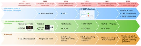
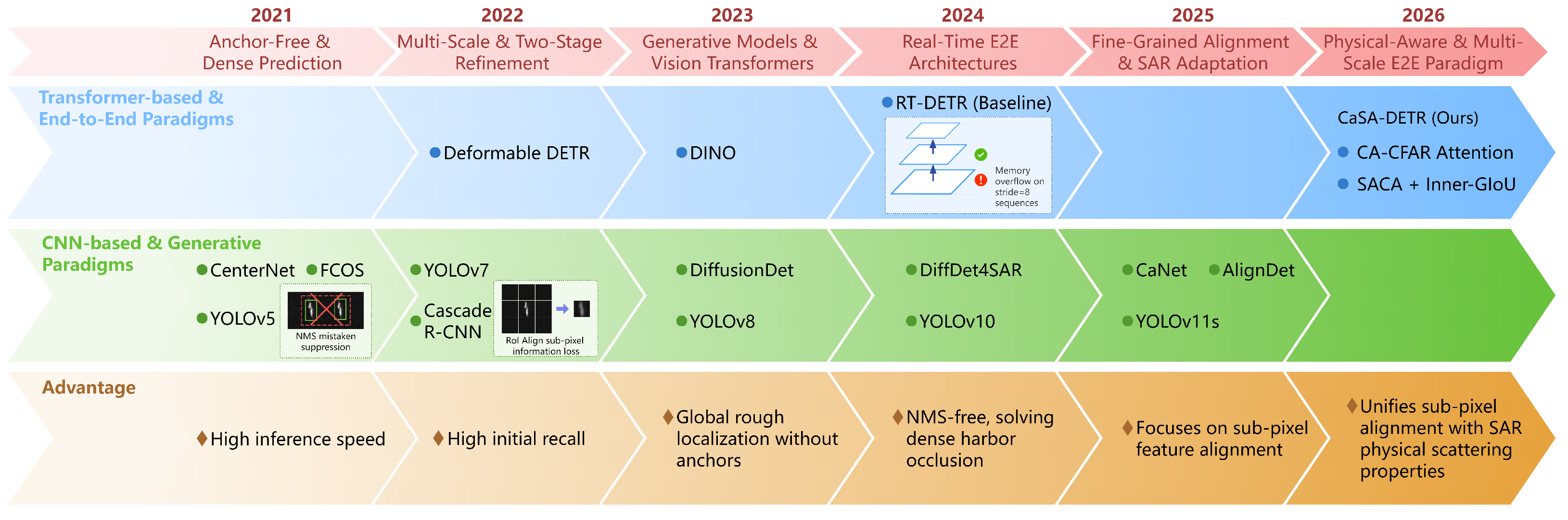
A synthetic aperture radar (SAR) can image the sea in all weather, day and night, over wide areas, and is used for maritime safety and monitoring. In maritime search and rescue, satellite SAR images can cover a search zone of hundreds of square kilometres, and fast ship detection can shorten the response time [1,2]. Automatic ship detection is also used to monitor illegal, unreported, and unregulated (IUU) fishing, to manage traffic in busy straits, and to watch offshore energy infrastructure. Figure 1 shows how representative deep-learning SAR ship detectors have developed, from early convolutional neural network (CNN) single-stage detectors to end-to-end Transformer frameworks.

Figure 1. Timeline of representative deep-learning methods for SAR ship detection, grouped by detection type. The method in this paper (2026, top-right) adds CFAR-Attention, SACA, and Inner-GIoU to RT-DETRv2.

In this paper, a small ship is a ship whose box in the source image is smaller than $32\times 32$ pixels (the Common Objects in Context (COCO) small-object limit). All ships in our benchmark meet this limit, and 35% are smaller than $16\times 16$ pixels. The annotation has one class (ship) and does not record ship type, length in metres, or hull material. The nine source datasets have different pixel spacings, so no common metric length can be given. The method uses only image intensity and does not depend on the hull material; its window and dilation settings were chosen for the 1024-pixel, stride-8 setting described below.

Small ship detection in SAR images differs from optical object detection in three ways.

First, the targets are very small. The median ship in our dataset covers about $360{\mathrm{px}}^2$ (an equivalent side of about 19 pixels in the source image). After a $256\times 256$ tile is resized to $1024\times 1024$, this is about 76 pixels, i.e., about 5 cells at stride-16 and about 2 cells at stride-32. Detectors that use global context only at coarse scales therefore get little information about such targets, so recall drops.

Second, ships appear as separate bright scattering points produced by two-bounce and corner-reflector effects, not as continuous textured shapes. Metal quay structures, buildings, and breaking waves in rough seas give returns that look like ships and cause false alarms. A detector can benefit from comparing each position with its local background.

Third, small boxes are sensitive to annotation offsets. For a ship with a 19-pixel side in the source image, a one-pixel shift of the boundary changes the box area by roughly 5 to 10%. Regression losses such as generalised intersection over union (GIoU) treat this uncertainty as valid supervision, which may bias the regression head; we did not measure this. Such a bias would matter most at strict intersection over union (IoU) thresholds, as measured by AP at IoU 0.75 (${\mathrm{AP}}_{75}$).

1.1. Related Work

CNN-based single-stage and two-stage detectors. RetinaNet [3] introduced the focal loss to handle foreground-background imbalance. SSD [4], Faster R-CNN [5], and YOLO-series detectors such as YOLOv8 [6] and YOLOv11 [7] are general detectors that have been applied to SAR ship detection. Single-stage detectors that use non-maximum suppression (NMS) can suppress neighbouring ships in crowded harbours.

Recent real-time detectors. D-FINE [8] refines boxes as probability distributions in a detection transformer (DETR) style detector, and YOLOv12 [9] uses area attention. Both are included in the comparison.

Diffusion-based detectors. DiffusionDet [10] and its SAR variant DiffDet4SAR [11], which was proposed for aircraft targets, use iterative denoising to build global context.

End-to-end Transformer detectors. DETR [12] and its successors (Deformable DETR [13], DINO [14], RT-DETR [15]) replace NMS with Hungarian matching, so neighbouring objects are not suppressed by NMS. RT-DETRv2 [16] improves the speed–accuracy trade-off. To limit the quadratic cost of self-attention, its encoder processes only stride-32 features, so stride-8 features do not go through the encoder.

Context-aware, tiny-object, and CFAR-based methods. CaNet [17] is a context-aware SAR ship detector that combines local multi-scale refinement with global context aggregation. NWD-based methods [18] replace the IoU with a Wasserstein distance for tiny objects and do not use SAR priors. Classical CFAR detectors [19] adapt to local background statistics, but they work on image pixels and are not trained with the detector. CFAR-guided networks pass CFAR results to the detector as input or as attention masks [20,21]. CFAR-Attention instead computes its local statistics on learned features inside the detector, so no external CFAR step is needed and the gate is trained with the rest of the network.

Attention mechanisms in SAR detection. Channel and spatial attention such as squeeze-and-excitation (SE) [22] and the convolutional block attention module (CBAM) [23] has been used in SAR ship detection to recalibrate feature responses. These modules compute their weights from channel statistics and do not compare a position with its spatial background. The module proposed here estimates a local mean and standard deviation in a sliding reference window, so its gate depends on the contrast between a position and its surroundings.

Physics-based polarimetric and joint-domain methods. Another line of work uses scattering physics directly. The general polarimetric correlation pattern (GPCP) [24] builds a joint-domain representation over polarisation, time, frequency, and space. Geometric and statistical features derived from it raise the target-to-clutter ratio of ships in Radarsat-2 and Gaofen-3 polarimetric SAR data. The scattering mechanism embedded network (SMEN) [25] embeds scattering mechanisms in a network that identifies corner-reflector arrays in polarimetric radar data. These methods need polarimetric or multi-domain measurements, which our single-channel intensity images do not provide. Our modules use intensity only and do not reproduce scattering decompositions. Using them together with joint-domain features is left for later work.

1.2. Contributions

We propose CaSA-DETR (Ca = CA-CFAR soft attention, SA = Scatter-Aware Context Aggregation), a detector built on RT-DETRv2 with the following contributions.

• CFAR-Attention. A differentiable local contrast normalisation inspired by cell-averaging CFAR. It estimates a local background mean and standard deviation from a reference window with a guard band, and turns the normalised response into a multiplicative soft gate. Zero-initialised projection weights give a gain close to one at the start ($\approx 1.035$). The module is applied to the stride-8 and stride-16 projected features that bypass the Transformer encoder. It is CFAR-inspired and does not give a constant false-alarm rate; Section 4.1 measures how far its response statistics depart from a Gaussian reference. Unlike CFAR-guided networks, the statistics are computed on learned features.
• Scatter-Aware Context Aggregation (SACA). Ship returns contain scattering centres, sidelobes, the hull, and surrounding clutter, which span different spatial scales. SACA uses four parallel dilated depthwise-separable branches with effective receptive fields of 3, 5, 9, and 17 feature cells, and a branch-adaptive gate that weights the four branch outputs for each sample. The dilation rates are a design choice, and Section 3.4 shows how AP depends on them.
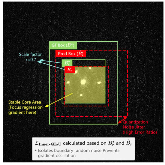
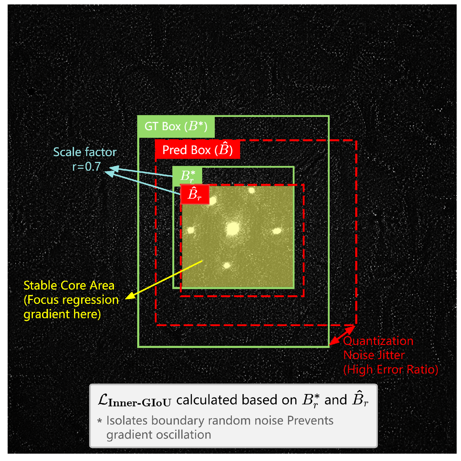
• Inner-GIoU. We apply Inner-GIoU [26] to small SAR ships: predicted and ground-truth boxes are shrunk by a factor $r=0.7$ before the GIoU regression loss is computed, so the gradient is taken on the inner part of each box. The effect of the shrink ratio is examined in Section 3.4.
• Experiments and dataset. A cross design and a full factorial ablation separate the effects of backbone, input size, and each module. We compare with recent detectors at the same input size and report complexity, latency, false alarms on ship-free images, validation-selected operating points, and overlap between data partitions. The dataset has 44,217 training images, 73,407 instances, and 100% small objects, assembled from nine public SAR repositories.

2. Materials and Methods

2.1. Dataset Description

2.1.1. Data Sources and Construction

The benchmark is built from nine publicly accessible SAR image repositories: HRSID [27], SSDD [28], SRSDD [29], AIR-SARShip [30], MSAR [31], RSDD [32], FUSAR-Ship [33], SAR-Ship-Dataset [34], and OpenSARShip [35]. These sources cover several sensors (Sentinel-1 interferometric wide (IW) and extra wide (EW) modes and high-resolution spotlight and stripmap modes), incidence angles, polarisations (VV, VH, HH), and regions including coastal harbours, shipping lanes, island-reef channels, and open ocean.

The raw collection was processed in seven steps.

• Empty image removal. Images with no annotated instances were discarded, so no empty images remain in any split.
• Degraded bounding-box filtering. Annotations with extreme aspect ratios (w/h < 0.10 or >10.0), zero area, or self-intersecting coordinates were removed. On the test split, the median aspect ratio is 1.04 and the 90th percentile is 2.80 (Table 1).
  Table 1. Test-split statistics (5527 images, 9245 instances). Training and validation splits have similar target-size and density distributions after the stratified split.

  Property	Value
  Total images/instances (test)	5527/9245
  Average instances per image	1.67
  Maximum instances in one image	76
  Dense images (≥5 targets)	233 (4.22%)
  Instances touching the image border (≤2 px)	1368 (14.80%)
  Instances $<32\times 32$ px (COCO small)	9245 (100%)
  Tiny sub-class (<$16\times 16$ ${\mathrm{px}}^2$)	3236 (35.0%)
  Small sub-class ($16\times 16$–$32\times 32$ ${\mathrm{px}}^2$)	6009 (65.0%)
  Median instance area	360 ${\mathrm{px}}^2$ (≈19 × 19 px)
  Mean instance area	413 ${\mathrm{px}}^2$
  90th-percentile area	825 ${\mathrm{px}}^2$
  Min/max instance area	4/1023 ${\mathrm{px}}^2$
  Dominant image resolution	256 × 256 (85.1% of images)
  Median aspect ratio (w/h)	1.04
  90th-percentile aspect ratio	2.80

• Severe truncation removal. Instances with more than 50% of the estimated box area outside the image were excluded. For a box cut along one axis, 50% outside is the point where the box centre leaves the image. The detector predicts box centres as normalised coordinates inside the image, so beyond this point less than half of the target is visible. We kept only targets that are at least half visible. Other cutoffs were not tested. Moderately truncated instances account for 14.68% of training instances.
• Statistics verification. After each filtering step, the minimum instance area, minimum side length, and maximum aspect ratio were logged before and after cleaning to check that valid tiny targets were not removed.
• Micro-target filtering. In images with original resolution above 1000 pixels, boxes with equivalent side length below 8 pixels ($\sqrt{wh}<8$) were removed, because such targets have too few pixels for reliable detection.
• Large-image tiling. Images larger than 500 pixels were tiled with a sliding window ($512\times 512$ pixels, 25% overlap). Tiles without target annotations were discarded.
• Annotation consistency. All bounding-box labels were converted to the COCO axis-aligned format and checked for coordinate consistency. No speckle filtering or other image denoising was applied; images are used as provided by the source datasets, apart from the tiling in step 6.

2.1.2. Dataset Splitting and Statistics

After quality control, instances were assigned to training, validation, and test splits by jointly stratifying on target category (ship), median instance area, proportion of tiny targets (<$16\times 16{\mathrm{px}}^2$), spatial density (instances per 10,000 image pixels), and source image resolution. The stratification keeps the target size and density distributions of the three partitions consistent.

The final dataset contains 55,271 images and 91,911 annotated instances: training (44,217 images; 73,407 instances), validation (5527 images; 9259 instances), and test (5527 images; 9245 instances). Table 1 summarises the main statistics.

Every annotated instance is below the COCO small-object threshold ($32\times 32=1024{\mathrm{px}}^2$), and 35% are tiny (<$16\times 16$). The median instance area of 360 ${\mathrm{px}}^2$ is about 0.55% of a typical 256 × 256 tile. The dataset is available from the corresponding author upon reasonable request.

Overlap between partitions. The split was made after tiling with 25% overlap, so neighbouring tiles of one scene can fall into different partitions. File names were anonymised during preprocessing and the scene of each tile cannot be recovered, so we searched for overlap by image content. Each test image was reduced to $256\times 256$ pixels and compared with all training and validation images. Whole-image comparison was used to find near-duplicates. To find tiling overlap, we compared the four border strips (25% of the side) and four corner blocks of each test image with the opposite strips and blocks of every training and validation image. We used the cosine similarity of pooled descriptors. Candidates were confirmed by a normalised correlation of at least 0.85. In total, 105 of the 5527 test images (1.90%), containing 213 of 9245 instances (2.30%), overlapped with training or validation images; 11 were whole-image near-duplicates and the others were border or corner overlaps. Of these images, 78 matched validation images and 43 matched training images, and some matched both. We evaluated five models (the ResNet-50-vd/640 baseline, the ResNet-50-vd/1024 baseline and full model, and the ResNet-101-vd/1024 baseline and full model) on the test set without these images, and the results changed only slightly. The procedure cannot detect overlap that is shifted, rescaled, or flipped, so 1.90% is the overlap it can find, not a proof that none remains. A split by scene would avoid the problem and is better for later versions of the dataset.

2.2. Overall Architecture

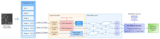
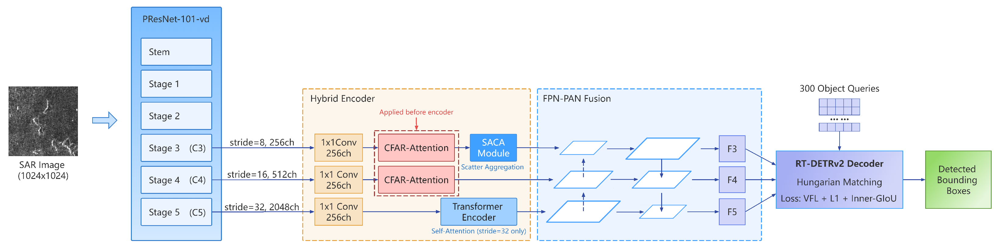
Figure 2 shows the proposed framework. It follows RT-DETRv2, which uses a ResNet backbone, a Hybrid Encoder with Feature Pyramid Network (FPN) and Path Aggregation Network (PAN) fusion, and a Transformer decoder with Hungarian matching. We make four changes to the baseline; the last three are the proposed components.

Figure 2. Architecture of CaSA-DETR. The ResNet-101-vd backbone produces features at strides 8, 16, and 32. CFAR-Attention is applied after input_proj on the stride-8 and stride-16 maps, which do not enter the Transformer encoder. SACA is then applied on the stride-8 map, before FPN fusion. The encoder uses only the stride-32 map.

• The backbone is changed from ResNet-50-vd to ResNet-101-vd, and the input resolution is raised from $640\times 640$ to $1024\times 1024$, which increases the pixel count by a factor of 2.56. Section 3.3 separates the effects of these two changes from those of the modules.
• CFAR-Attention is inserted after the channel projection layer (input_proj) of the Hybrid Encoder and acts on the two projected feature maps that bypass the Transformer encoder (stride-8 and stride-16). The encoder itself operates only on the stride-32 projection (use_encoder_idx=[2]).
• SACA is applied to the stride-8 feature after CFAR-Attention and before FPN fusion. It acts only on the stride-8 branch.
• The regression loss is replaced with Inner-GIoU.

2.3. CA-CFAR Soft Attention Module (CFAR-Attention)

2.3.1. Motivation of CFAR-Attention

The cell-averaging CFAR (CA-CFAR) detector is a standard tool in radar signal processing. For a cell under test, it estimates the background level from a surrounding reference window that excludes a guard band, and it declares a detection when the cell exceeds a threshold $T=\eta ·{\mu }_{\mathrm{bg}}$, where ${\mu }_{\mathrm{bg}}$ is the estimated local background mean and $\eta$ sets the desired false-alarm rate.

We use the same local-contrast idea on learned feature maps: a position whose response is high relative to its local background is more likely to belong to a ship. We chose the cell-averaging form because its background estimate is a local mean and variance, which box filters compute directly and through which gradients pass. Order-statistic CFAR needs a sort inside every window, and the greatest-of and smallest-of variants address clutter edges and interfering targets; these are harder to put into a convolutional network. We did not try them, so we do not claim that the cell-averaging form is the best choice. The resulting module is CFAR-inspired and is not a CFAR detector. It keeps the reference window and guard band, replaces the hard threshold with a soft gate, and computes its statistic on a learned single-channel response instead of SAR power. Feature responses do not follow the clutter models used to derive CFAR thresholds, so the module has no false-alarm-rate guarantee; Section 4.1 measures the deviation.

2.3.2. Design of CFAR-Attention

Let $\mathbf{X}\in {\mathbb{R}}^{B\times C\times H\times W}$ be the input feature tensor.

Step 1: single-channel response map. A learnable $1\times 1$ convolution $f_{\theta }$ compresses the C-channel feature to a scalar response map:

$$s=f_{\theta }\left(\mathbf{X}\right)\in {\mathbb{R}}^{B\times 1\times H\times W}.$$

(1)

The weights of $f_{\theta }$ are zero-initialised, so $s\approx 0$ at the start of training, the gate weight in Equation (3) is about $\sigma \left(0\right)=0.5$, and the initial gain is $1+\alpha ·0.5\approx 1.035$.

Step 2: background statistics. The reference window is approximated with box-filter convolutions. Let ${\mathbf{1}}_k$ denote a $k\times k$ all-ones kernel. For outer window size w and guard size g:

$$\widehat{\mu }={\displaystyle \frac{{\mathbf{1}}_w\ast s-{\mathbf{1}}_g\ast s}{w^2-g^2}},\widehat{\sigma }=\sqrt{\max \left({\displaystyle \frac{{\mathbf{1}}_w\ast s^2-{\mathbf{1}}_g\ast s^2}{w^2-g^2}}-{\widehat{\mu }}^2,0\right)+\epsilon },$$

(2)

where ∗ denotes 2D convolution with zero-padding of half the window width ($\lfloor w/2\rfloor =3$ cells) and $\epsilon ={10}^{-6}$. For the default configuration ($w=7$, $g=3$), the number of reference cells is $n_r=w^2-g^2=49-9=40$. The $\max (·,0)$ clamp keeps the variance non-negative, because rounding errors can make it slightly negative when s is almost constant over the window. The computation is done in float32 (explicit cast under AMP), since the $7\times 7$ box-filter sums can overflow in float16.

At the feature-map border, zero-padding means that the box filter covers fewer valid cells than $n_r$ while the denominator stays at $n_r=40$, so the estimated mean is biased towards zero within $\lfloor w/2\rfloor =3$ feature cells of the border (24 input pixels at stride-8 and 1024 × 1024 input). This matters for targets near the image border, because 14.80% of the test instances touch it (Table 1). We measure the Recall of border-touching targets directly in Section 3.6.

Step 3: soft detection weight. To avoid hard switching on uniform backgrounds where $\widehat{\sigma }\to 0$, $\widehat{\sigma }$ is clamped to a minimum of $0.05$ before the division. This floor keeps the normalised statistic $(s-\widehat{\mu })/\widehat{\sigma }$ bounded when $\widehat{\sigma }\to 0$, for example at initialisation, where s is zero everywhere. The value was not tuned, and its effect on AP was not measured. The normalised statistic is then passed through a sigmoid:

$$w=\sigma \left({\displaystyle \frac{k·(s-\widehat{\mu })}{\widehat{\sigma }}}-\tau \right),$$

(3)

where $k=1.0$ sets the slope and $\tau =0.0$ the threshold offset. Positions whose response is far above the local mean have $w\to 1$ and a gain of $(1+\alpha )\approx 1.07$, and positions that match the local mean have $w\approx 0.5$ and a gain of $1+0.5\alpha \approx 1.035$.

Step 4: multiplicative gate.

$$\mathrm{CFAR}\left(\mathbf{X}\right)=\mathbf{X}·(1+\alpha ·w),$$

(4)

where $\alpha =0.07$ is the amplification strength. The gain lies in $[1.00,1.07]$, so no activation is attenuated. The gate acts as a mild reweighting of target-like positions relative to the rest of the feature map.

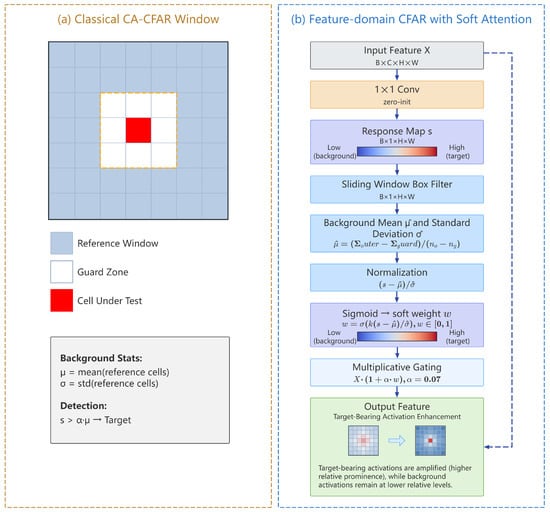
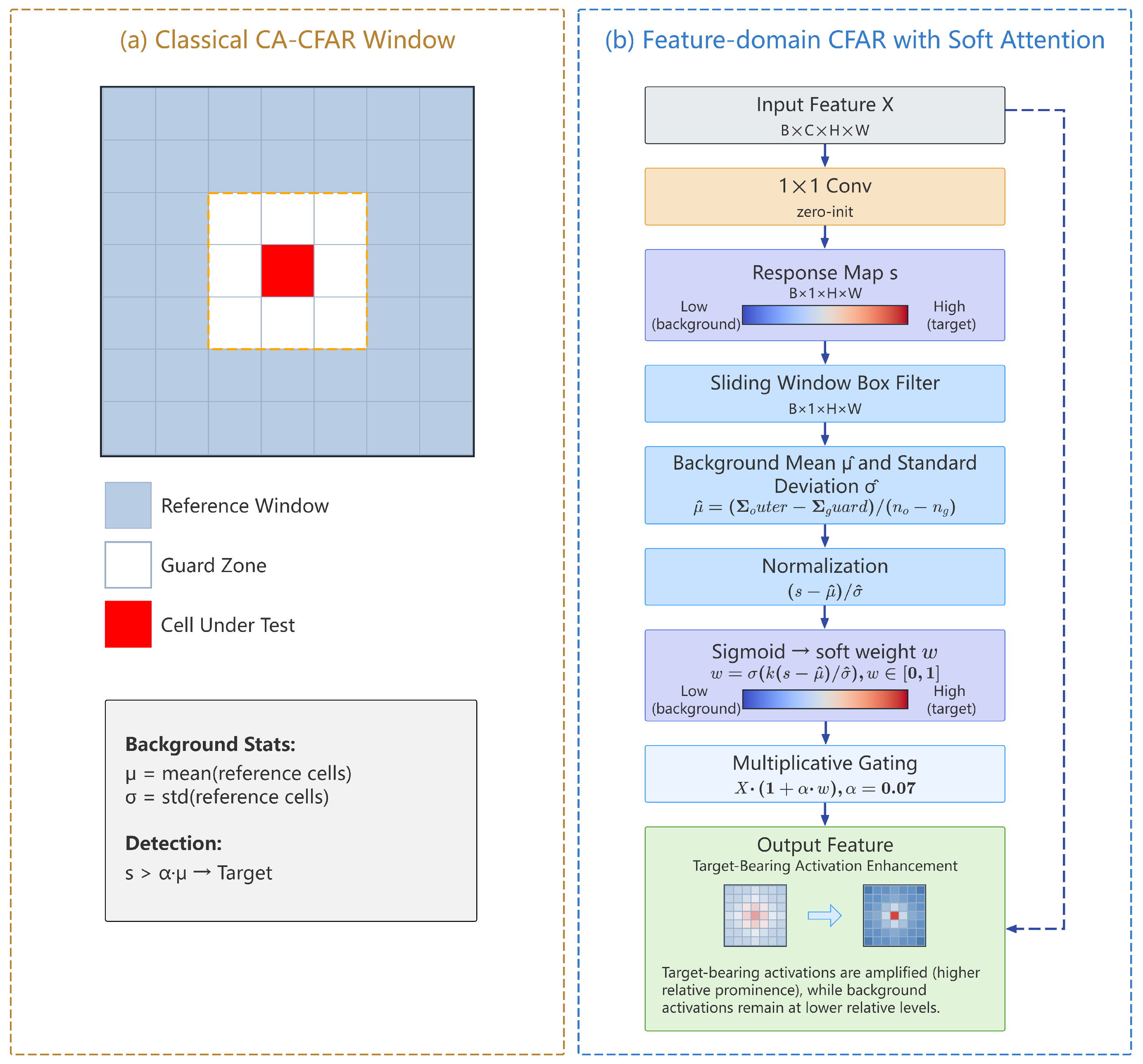
Application position. CFAR-Attention is applied to the two projected features that bypass the Transformer encoder: stride-8 (${\mathbf{X}}_{C_3}$) and stride-16 (${\mathbf{X}}_{C_4}$). The default RT-DETRv2 encoder operates on stride-32 features only (use_encoder_idx=[2]). We chose these levels so that the encoder input stays unchanged; alternative placements were not re-evaluated under the final training protocol. The mechanism is illustrated in Figure 3.

Figure 3. CFAR-Attention. (a) CA-CFAR reference window (outer window $7\times 7$, guard zone $3\times 3$). (b) Use on feature maps: a $1\times 1$ convolution produces a response map, a sliding window estimates the local mean and standard deviation, and a sigmoid gate multiplies the feature.

2.4. Scatter-Aware Context Aggregation Module (SACA)

2.4.1. Motivation of SACA

Ships in SAR images show up as separate, localised scattering points and not as continuous textured shapes. A ship return usually contains bright scattering centres, sidelobes, the hull, and the surrounding sea clutter. These parts cover different spatial scales, and vessel sizes in SAR images vary widely [36]. One kernel size does not cover all of these scales.

SACA aggregates context with parallel dilated convolutions, in the same spirit as atrous spatial pyramid pooling (ASPP) [37], but with depthwise-separable branches and a per-sample gate over the branches. At stride-8, dilation rates $\{1,2,4,8\}$ give effective receptive fields of $\{3\times 3,5\times 5,9\times 9,17\times 17\}$ feature cells, i.e., roughly 24 to 136 input pixels at 1024 × 1024 input. These values are a design choice that covers the range from a scattering centre to the local clutter neighbourhood. They were not derived from an electromagnetic scattering model, and Section 3.4 reports how the results depend on them.

2.4.2. Design of SACA

Let $\mathbf{X}\in {\mathbb{R}}^{B\times C\times H\times W}$ be the input feature ($C=256$, $H=W=128$ at stride-8 and 1024 px input). Each of the four branches applies a depthwise dilated convolution followed by a pointwise projection, both with batch normalisation (BN) and ReLU:

$${\mathbf{Z}}_k=\mathrm{ReLU}\left(\mathrm{BN}\left({\mathrm{PW}}_{1\times 1}\left(\mathrm{ReLU}\left(\mathrm{BN}\left({\mathrm{DWConv}}_{3\times 3}^{d_k}\left(\mathbf{X}\right)\right)\right)\right)\right)\right),d_k\in \{1,2,4,8\},$$

(5)

where ${\mathrm{DWConv}}_{3\times 3}^d$ is a depthwise (grouped) $3\times 3$ convolution with dilation d, and ${\mathrm{PW}}_{1\times 1}$ is a pointwise ($1\times 1$, channel-mixing) convolution. The effective receptive field of branch k is $(2d_k+1)\times (2d_k+1)\in \{3\times 3,5\times 5,9\times 9,17\times 17\}$, and each ${\mathbf{Z}}_k\in {\mathbb{R}}^{B\times C\times H\times W}$.

Branch-adaptive gating. Unlike standard SE attention, which takes the input feature $\mathbf{X}$, the gate takes the concatenated branch outputs, so that the weights depend on what each branch actually produces:

$${\mathbf{Z}}_{\mathrm{cat}}=\mathrm{Cat}[{\mathbf{Z}}_1,{\mathbf{Z}}_2,{\mathbf{Z}}_3,{\mathbf{Z}}_4]\in {\mathbb{R}}^{B\times 4C\times H\times W},$$

(6)

$$\mathbf{w}=\sigma \left({\mathbf{W}}_2\mathrm{ReLU}\left({\mathbf{W}}_1\mathrm{GAP}\left({\mathbf{Z}}_{\mathrm{cat}}\right)\right)\right)\in {\mathbb{R}}^{B\times 4},$$

(7)

where ${\mathbf{W}}_1\in {\mathbb{R}}^{s\times 4C}$, ${\mathbf{W}}_2\in {\mathbb{R}}^{4\times s}$, and $s=\max (4C/r,4)=64$ (reduction ratio $r=16$, $C=256$); both are implemented as $1\times 1$ convolutions after global average pooling. The output contains four branch-specific scalar weights: each $w_k={\mathbf{w}}_{:,k}\in {\mathbb{R}}^B$ is a per-sample scalar for branch k, computed from all four branch outputs and broadcast over $C\times H\times W$.

Weighted fusion and residual.

$$\mathrm{SACA}\left(\mathbf{X}\right)=\mathbf{X}+\mathrm{BN}\left({\mathrm{PW}}_{1\times 1}\left({\displaystyle \sum _{k=1}^4}{w}_k·{\mathbf{Z}}_k\right)\right).$$

(8)

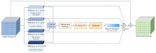
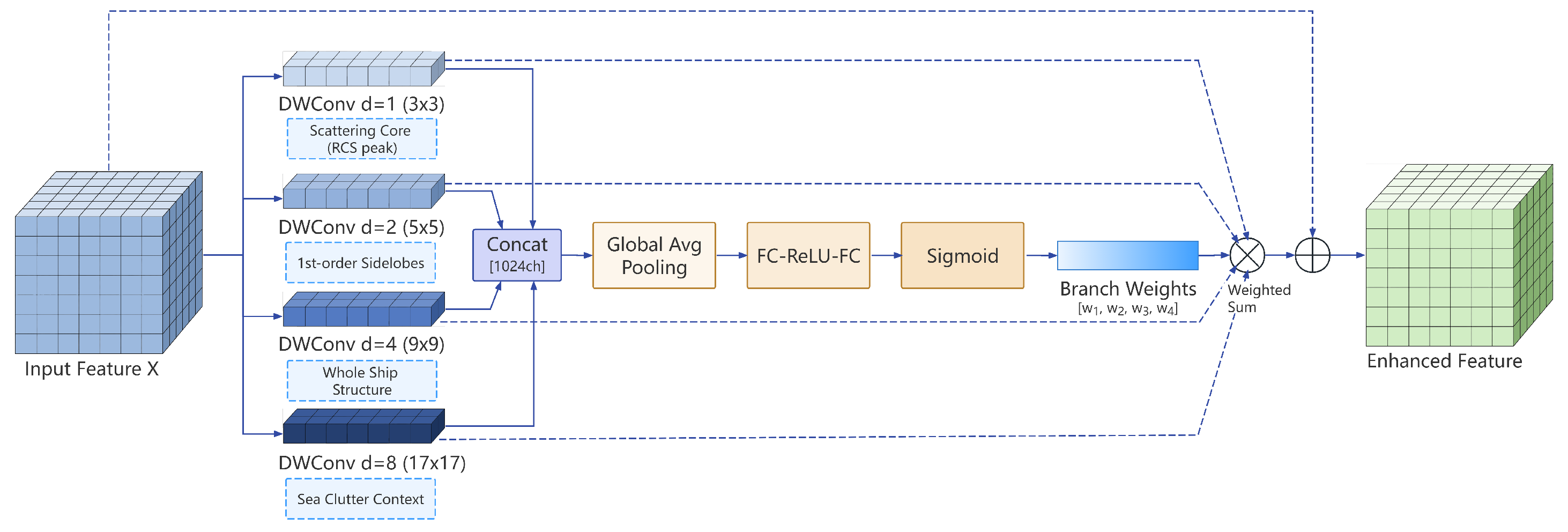
Table 2 lists the layer-wise tensor shapes and parameter counts, and Figure 4 illustrates the module.

Table 2. SACA layer shapes and parameter counts ($C=256$, $H=W=128$). Convolutions have no bias; BN parameters are included.

Layer	Output Shape	#Params	Notes
${\mathrm{DWConv}}_{3\times 3}^{d_k}$ ($\times 4$)	$[B,C,H,W]$ each	$4\times 9C=9216$	groups = C (depthwise)
BN+ReLU ($\times 4$)	$[B,C,H,W]$	$4\times 2C=2048$
PW ${\mathrm{Conv}}_{1\times 1}$ ($\times 4$)	$[B,C,H,W]$	$4\times C^2=\mathrm{262,144}$	channel-mixing
BN+ReLU ($\times 4$)	$[B,C,H,W]$	$4\times 2C=2048$
Concatenate	$[B,4C,H,W]$	0
GAP	$[B,4C,1,1]$	0
${\mathbf{W}}_1$: ${\mathrm{Conv}}_{1\times 1}(4C\to s)$	$[B,64,1,1]$	$4C\times s=\mathrm{65,536}$	$s=64$
${\mathbf{W}}_2$: ${\mathrm{Conv}}_{1\times 1}(s\to 4)$	$[B,4,1,1]$	$s\times 4=256$	4 branch scalars
Weighted sum ${\sum }_k{w}_k{\mathbf{Z}}_k$	$[B,C,H,W]$	0
Proj ${\mathrm{Conv}}_{1\times 1}(C\to C)$	$[B,C,H,W]$	$C^2=\mathrm{65,536}$
Proj BN	$[B,C,H,W]$	$2C=512$
Total		407,296	$\approx 0.41$ M

Figure 4. SACA module. Four depthwise-separable branches with dilation $d\in \{1,2,4,8\}$ produce features ${\mathbf{Z}}_k$. The concatenated outputs go through global average pooling and two $1\times 1$ convolutions to give four scalar weights $w_k$. The weighted sum is projected back to C channels and added to the input.

SACA is applied to the stride-8 feature after CFAR-Attention and before FPN fusion. CFAR-Attention covers both non-encoder levels, whereas SACA acts only on the stride-8 CFAR-processed feature, so the fine-grained branch passes through the two modules in sequence.

2.5. Inner-GIoU Loss

2.5.1. Motivation of Inner-GIoU

For ships with a median side of about 19 pixels in the source image, a one-pixel shift of the annotated boundary changes the box area by roughly 5 to 10%. The standard GIoU loss [38] treats this boundary uncertainty as valid supervision, which may bias the regression head. The one-pixel shift is only an estimate. We did not perturb the boxes in a controlled test; results for different shrink ratios are in Section 3.4.

2.5.2. Formulation

Inner-GIoU shrinks the predicted box $\widehat{B}$ and the ground-truth box $B^{*}$ towards their centres by a scale factor r:

$${\widehat{B}}_r=\mathrm{Scale}(\widehat{B},r),B_r^{*}=\mathrm{Scale}(B^{*},r),$$

(9)

and computes the GIoU loss on the contracted boxes:

$${\mathcal{L}}_{\mathrm{InnerGIoU}}=1-\mathrm{IoU}({\widehat{B}}_r,B_r^{*})+{\displaystyle \frac{|C_r\setminus ({\widehat{B}}_r\cup B_r^{*})|}{|C_r|}},$$

(10)

where $C_r$ is the minimum enclosing rectangle of ${\widehat{B}}_r$ and $B_r^{*}$. With $r=0.7$, the loss uses the inner $r^2=49\%$ of each box area. The shrinkage is illustrated in Figure 5.

Figure 5. Inner-GIoU. The predicted box $\widehat{B}$ and the ground-truth box $B^{*}$ are shrunk by $r=0.7$ towards their centres, and the loss is computed on the inner boxes ${\widehat{B}}_r$ and $B_r^{*}$.

2.6. Training Strategy

Training proceeds in two phases.

Phase 1: standard training (30 epochs). We use the AdamW optimiser [39] with a backbone learning rate of $5\times {10}^{-6}$ and an encoder/decoder learning rate of $5\times {10}^{-5}$, MultiStepLR decay by a factor of 0.1 at epoch 24, and a 200-iteration linear warm-up. The batch size is 8 and automatic mixed precision (AMP) is used. Data augmentation consists of random photometric distortion, random zoom-out, random IoU crop ($p=0.8$), random horizontal flip, and a fixed resize to the input size ($1024\times 1024$; $640\times 640$ for the 640-pixel baselines). These augmentations are applied online during training only.

Phase 2: extended fine-tuning (20 epochs). Starting from the best Phase-1 checkpoint, the backbone learning rate is $1\times {10}^{-6}$ and the remaining learning rate is $1\times {10}^{-5}$ without scheduler decay, and the optimiser state is reset (resume_exclude = [optimizer, lr_scheduler]). The total training length is 50 epochs.

The optimiser settings follow the public RT-DETRv2 ResNet-50-vd configuration, in which the learning rates are $1\times {10}^{-4}$ (encoder and decoder) and $1\times {10}^{-5}$ (backbone). We used $5\times {10}^{-5}$ and $5\times {10}^{-6}$, shortened the warm-up to 200 iterations, and added a learning-rate decay at epoch 24 to fit 30 epochs. The Phase-2 learning rates are one fifth of the Phase-1 values. We did not search over these values.

On the validation set, E1 and E5 still gained AP between epoch 30 (56.34% and 60.19%) and epoch 50 (56.85% and 60.92%); the best checkpoints were at epochs 41 and 46.

3. Results

3.1. Experimental Setup

Hardware. All experiments were run on a single NVIDIA GeForce RTX 5090 D GPU (32 GB GDDR7, Windows 10) with PyTorch 2.7.0 and CUDA 12.8, with AMP mixed-precision training enabled.

Model complexity. The RT-DETRv2 baseline with a ResNet-50-vd backbone has 42.7 M trainable parameters (42,700,515). Switching to ResNet-101-vd raises this to 61.6 M (61,640,419), an increase of 18.9 M that comes entirely from the deeper backbone. CFAR-Attention adds one $1\times 1$ convolution (256 channels to 1, no bias) per non-encoder level, i.e., $2\times 256=512$ parameters, and SACA adds 0.41 M (407,296 in total). The full model (E5) has 62.0 M parameters (62,048,227), which is $+0.66\%$ over the ResNet-101-vd baseline. All parameter counts in this paper are trainable parameters of the training graph. The same modules add 407,808 parameters to the ResNet-50-vd model (42,700,515 to 43,108,323).

Evaluation protocol. Evaluation uses the standard COCO metrics on the test split (5527 images, 9245 instances) with faster-coco-eval. The confidence threshold is fixed at 0.001 so that the full precision-recall (P-R) curve is covered. Precision, Recall, and F1 are reported at the working point with maximum F1 on the P-R curve at IoU = 0.50 (area = all, maxDets = 100). This point is read from the interpolated curve of the test set itself, so Recall takes values in steps of 0.01. Section 3.6 repeats the evaluation with a confidence threshold chosen on the validation set.

Reproducibility. The full model (E5) was trained twice with identical configurations and different random seeds (the second run used seed 42). The two runs gave AP 60.75% and 60.68%, ${\mathrm{AP}}_{50}$ 92.27% and 92.32%, ${\mathrm{AP}}_{75}$ 63.95% and 63.84%, ${\mathrm{AP}}_s$ 60.78% and 60.71%, Precision 91.23% and 91.19%, Recall 89.00% in both, and F1 90.10% and 90.08%. The largest difference on any metric is 0.11. All tables report the first run. Only two seeds were run, so differences of about 0.2 AP or less between single runs should be treated with caution.

Competing methods. We compare against RetinaNet, YOLOv8, YOLOv11, Faster R-CNN, DiffusionDet, DiffDet4SAR, CaNet, DINO, RT-DETR, and RT-DETRv2 (baseline), and also D-FINE and YOLOv12. All methods were re-trained by the authors on the same dataset splits and hardware using public implementations. Backbones were initialised following each method’s public implementation, and all methods were trained on the SAR split for 50 epochs with best-checkpoint selection by validation AP. The original hyperparameters of each method were kept except for the number of epochs, and the 50-epoch schedule was not tuned for individual methods. Backbones and input sizes differ between methods and are listed in Table 3. The first block of Table 3 gives the results of the original protocol, and the second block gives the methods re-trained at 1024 by 1024 input, so that every method not already trained at 1024 is also compared at that size.

Table 3. Comparison with other detectors on the SAR small-ship test set (5527 images, 9245 instances). All methods were trained for 50 epochs; the checkpoint with the highest validation AP is reported. The first block is the original protocol; the second block is re-trained at 1024 × 1024. Metrics in %. Best in each column in bold. †: our method.

Method	Backbone	Input	AP	${\mathrm{AP}}_{50}$	${\mathrm{AP}}_{75}$	${\mathrm{AP}}_{\mathit{s}}$	Prec.	Recall	F1
RetinaNet	CSPResNet	640	44.32	75.33	43.92	44.43	79.17	68.00	73.16
CaNet	ResNet-50 + FPN	1024	50.55	86.58	51.37	50.28	84.31	84.00	84.15
DiffusionDet	ResNet-50 + FPN	1024	50.63	88.62	51.01	50.19	90.43	84.00	87.10
YOLOv8	CSPDarknet	640	51.25	86.50	52.66	51.05	84.25	82.00	83.12
YOLOv11	YOLO11	640	52.42	87.59	54.13	52.55	86.33	83.00	84.63
Faster R-CNN	ResNet-50	800	52.69	87.56	54.68	52.52	84.94	85.00	84.97
DINO	ResNet-50 + FPN	1024	52.94	87.46	54.79	52.84	86.12	85.00	85.56
DiffDet4SAR	ResNet-50 + FPN	1024	53.11	88.74	54.63	52.90	91.13	85.00	87.96
RT-DETR	ResNet-50-vd	800	54.40	89.91	57.10	54.21	87.67	86.00	86.83
RT-DETRv2 (baseline)	ResNet-50-vd	640	56.71	90.76	60.18	56.60	88.85	87.00	87.92
Ours †	ResNet-101-vd	1024	60.75	92.27	63.95	60.78	91.23	89.00	90.10
Re-trained at 1024 × 1024 input
RetinaNet	CSPResNet	1024	46.58	77.82	45.73	46.45	81.11	71.00	75.72
YOLOv8	CSPDarknet	1024	52.94	88.06	54.10	52.75	85.84	83.00	84.40
YOLOv11	YOLO11	1024	54.12	89.26	55.81	53.77	87.19	85.00	86.08
YOLOv12	YOLOv12	1024	52.49	87.79	53.91	52.14	85.08	83.00	84.03
Faster R-CNN	ResNet-50	1024	53.43	88.19	55.30	53.28	85.71	85.00	85.35
RT-DETR	ResNet-50-vd	1024	55.59	90.43	58.32	55.04	88.58	87.00	87.78
D-FINE	HGNetv2	1024	56.79	90.80	59.22	55.93	89.01	88.00	88.50
RT-DETRv2	ResNet-50-vd	1024	59.03	91.22	62.08	58.99	89.81	89.00	89.39
Ours †	ResNet-50-vd	1024	60.47	92.08	63.56	60.52	91.09	89.00	90.03
Ours (R101) vs. RT-DETRv2 baseline (R50/640)			+4.04	+1.51	+3.77	+4.18	+2.38	+2.00	+2.18
Ours (R101) vs. D-FINE			+3.96	+1.47	+4.73	+4.85	+2.22	+1.00	+1.60
Ours (R50) vs. D-FINE			+3.68	+1.28	+4.34	+4.59	+2.08	+1.00	+1.53

The D-FINE rows compare with that method at 1024 input. RT-DETRv2 in the second block is the same-family baseline (59.03 AP); the R50 full model is 1.44 AP above it. Among the other methods, DiffDet4SAR has the highest Precision (91.13%). F1 is the peak of the P-R curve at IoU = 0.5. Italic rows give the differences between our model and the method named in each row, in percentage points.

3.2. Comparison with Other Detectors

Table 3 gives the quantitative comparison on the test set.

(1) Overall performance. The full model reaches AP 60.75%, 4.04 AP above the original RT-DETRv2 baseline and 3.96 AP above D-FINE (56.79%) at the same 1024 input. Because our model uses ResNet-101-vd, we also report a ResNet-50-vd variant: 60.47%, 3.68 AP above D-FINE and 1.44 AP above ResNet-50-vd RT-DETRv2 at the same input (59.03%). Re-training at 1024 raised the AP of every method that was first trained at a smaller input (by 0.74 to 2.32 AP). Our two variants still have higher AP than those re-trained methods.

(2) Where the gain over the original baseline comes from. Of the 4.18 AP between the same-protocol ResNet-50-vd/640 baseline (56.57%) and the full model, 2.46 AP comes from raising the input size to 1024, 0.44 AP from the ResNet-101-vd backbone, and 1.28 AP from the three modules; Section 3.3 gives the details. The modules account for about a third of the improvement, and the input resolution for the larger part.

(3) ${AP}_{75}$. ${\mathrm{AP}}_{75}$ is 63.95%, 4.73 points above D-FINE (59.22%). Part of this gap comes from input size and backbone, as shown in Section 3.3; Inner-GIoU also contributes.

(4) Recall and precision. The model reaches Recall 89.00%, which is 1.00 point above D-FINE (88.00%) and 3.00 points above RT-DETR at its original input (86.00%). At 1024 input, the YOLO detectors, which use NMS, reach a Recall of 83.00% (YOLOv8 and YOLOv12) and 85.00% (YOLOv11), below RT-DETR (87.00%) and D-FINE (88.00%). DiffDet4SAR has the highest external Precision (91.13%) at a Recall of 85.00%, which gives F1 87.96%; our model has Precision 91.23% and Recall 89.00% (F1 90.10%). The Precision difference to DiffDet4SAR (0.10 points) is within run-to-run variation, whereas the Recall difference (4.00 points) is larger than that variation.

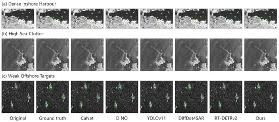
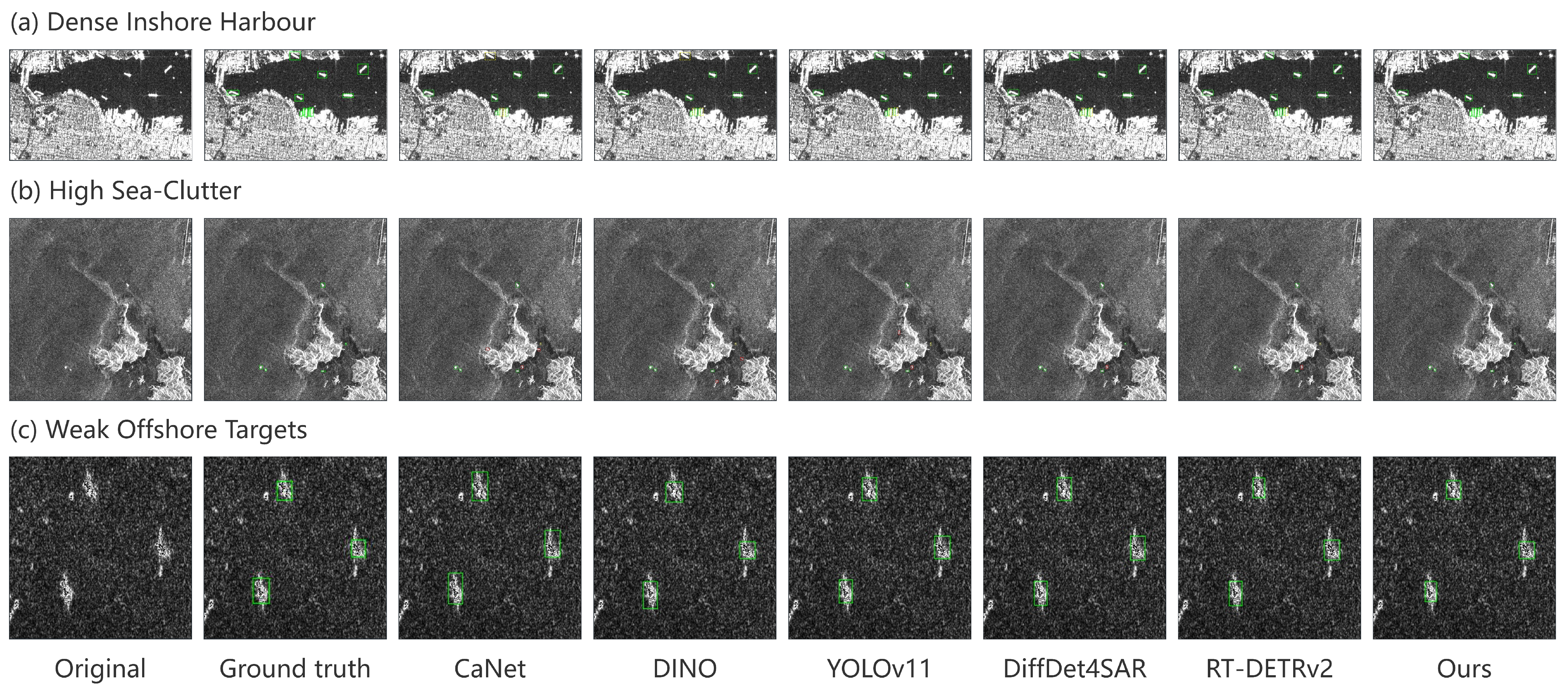
Figure 6 compares the original-protocol methods on three scenes: a dense harbour, sea clutter, and weak offshore ships.

Figure 6. Visual comparison on three SAR scenes (methods as in the original protocol of Table 3). Columns left to right: (1) SAR image, (2) ground truth, (3) CaNet, (4) DINO, (5) YOLOv11, (6) DiffDet4SAR, (7) RT-DETRv2, (8) Ours. Row 1: dense harbour; yellow boxes mark misses in the other methods. Row 2: sea clutter; red boxes mark false alarms. Row 3: weak offshore ships; several other methods produce oversized boxes.

3.3. Backbone, Resolution and Module Effects

In the original ablation, the backbone and the input size change together between E1 and E2, so their effects cannot be separated. Table 4 trains the baseline and the full model with two backbones and two input sizes under one protocol (batch size 8, 30 + 20 epochs). The R50/640 baseline reproduces the original E1 to within 0.14 AP (56.57% against 56.71%).

Table 4. Cross of backbone, input size, and modules under a single training protocol. “None” denotes the RT-DETRv2 baseline; “Full” denotes Inner-GIoU + CFAR-Attention + SACA. Config labels (S1a, X2a, …) are used consistently in the following tables. All metrics in %.

Config	Backbone	Input	Modules	AP	${\mathrm{AP}}_{50}$	${\mathrm{AP}}_{75}$	${\mathrm{AP}}_{\mathit{s}}$	Prec.	F1
S1e	ResNet-50-vd	640	None	56.57	90.49	60.16	56.45	88.63	87.81
S1b	ResNet-101-vd	640	None	57.12	90.69	60.85	56.94	88.79	88.39
S1c	ResNet-50-vd	640	Full	57.54	91.33	60.95	57.24	89.47	88.73
S1a	ResNet-50-vd	1024	None	59.03	91.22	62.08	58.99	89.81	89.39
E2	ResNet-101-vd	1024	None	59.47	91.52	62.88	59.54	90.13	89.56
S1d	ResNet-50-vd	1024	Full	60.47	92.08	63.56	60.52	91.09	90.03
E5	ResNet-101-vd	1024	Full	60.75	92.27	63.95	60.78	91.23	90.10

Recall is 87.00 (S1e), 88.00 (S1b, S1c), and 89.00 (all 1024-pixel configurations). E2 and E5 are the original ablation rows of Table 5.

Table 4. Cross of backbone, input size, and modules under a single training protocol. “None” denotes the RT-DETRv2 baseline; “Full” denotes Inner-GIoU + CFAR-Attention + SACA. Config labels (S1a, X2a, …) are used consistently in the following tables. All metrics in %.

Config	Backbone	Input	Modules	AP	${\mathrm{AP}}_{50}$	${\mathrm{AP}}_{75}$	${\mathrm{AP}}_{\mathit{s}}$	Prec.	F1
S1e	ResNet-50-vd	640	None	56.57	90.49	60.16	56.45	88.63	87.81
S1b	ResNet-101-vd	640	None	57.12	90.69	60.85	56.94	88.79	88.39
S1c	ResNet-50-vd	640	Full	57.54	91.33	60.95	57.24	89.47	88.73
S1a	ResNet-50-vd	1024	None	59.03	91.22	62.08	58.99	89.81	89.39
E2	ResNet-101-vd	1024	None	59.47	91.52	62.88	59.54	90.13	89.56
S1d	ResNet-50-vd	1024	Full	60.47	92.08	63.56	60.52	91.09	90.03
E5	ResNet-101-vd	1024	Full	60.75	92.27	63.95	60.78	91.23	90.10

Recall is 87.00 (S1e), 88.00 (S1b, S1c), and 89.00 (all 1024-pixel configurations). E2 and E5 are the original ablation rows of Table 5.

Table 5. Ablation on the SAR test set (all configurations: 50 epochs, best checkpoint). E1 to E5 add one component to the previous row. The last four rows (X2a to X2d) are the other combinations of the three modules on the same ResNet-101-vd/1024 baseline. ✓: active; —: not used. All metrics in %.

Config	Backbone +Res.	Inner- GIoU	CFAR- Attn	SACA	AP	${\mathrm{AP}}_{50}$	${\mathrm{AP}}_{75}$	${\mathrm{AP}}_{\mathit{s}}$	Prec.	Recall	F1
E1 (Baseline)	R50/640	—	—	—	56.71	90.76	60.18	56.60	88.85	87.00	87.92
E2 (+Backbone)	R101/1024	—	—	—	59.47	91.52	62.88	59.54	90.13	89.00	89.56
E3 (+Inner-GIoU)	R101/1024	✓	—	—	59.87	91.93	63.24	60.09	90.72	89.00	89.85
E4 (+CFAR-Attn)	R101/1024	✓	✓	—	60.40	92.10	64.13	60.57	91.07	89.00	90.02
E5 (+SACA, Ours)	R101/1024	✓	✓	✓	60.75	92.27	63.95	60.78	91.23	89.00	90.10
X2a (CFAR only)	R101/1024	—	✓	—	60.02	91.95	63.56	60.18	90.77	89.00	89.88
X2b (SACA only)	R101/1024	—	—	✓	59.73	91.78	63.04	59.85	90.42	89.00	89.70
X2c (Inner + SACA)	R101/1024	✓	—	✓	60.15	92.03	63.38	60.30	90.71	89.00	89.85
X2d (CFAR + SACA)	R101/1024	—	✓	✓	60.19	91.90	63.78	60.28	90.80	89.00	89.90

E1 uses the original R50-vd/640 configuration. Table 4 separates backbone and resolution. Bold: the full model (E5).

Table 5. Ablation on the SAR test set (all configurations: 50 epochs, best checkpoint). E1 to E5 add one component to the previous row. The last four rows (X2a to X2d) are the other combinations of the three modules on the same ResNet-101-vd/1024 baseline. ✓: active; —: not used. All metrics in %.

Config	Backbone +Res.	Inner- GIoU	CFAR- Attn	SACA	AP	${\mathrm{AP}}_{50}$	${\mathrm{AP}}_{75}$	${\mathrm{AP}}_{\mathit{s}}$	Prec.	Recall	F1
E1 (Baseline)	R50/640	—	—	—	56.71	90.76	60.18	56.60	88.85	87.00	87.92
E2 (+Backbone)	R101/1024	—	—	—	59.47	91.52	62.88	59.54	90.13	89.00	89.56
E3 (+Inner-GIoU)	R101/1024	✓	—	—	59.87	91.93	63.24	60.09	90.72	89.00	89.85
E4 (+CFAR-Attn)	R101/1024	✓	✓	—	60.40	92.10	64.13	60.57	91.07	89.00	90.02
E5 (+SACA, Ours)	R101/1024	✓	✓	✓	60.75	92.27	63.95	60.78	91.23	89.00	90.10
X2a (CFAR only)	R101/1024	—	✓	—	60.02	91.95	63.56	60.18	90.77	89.00	89.88
X2b (SACA only)	R101/1024	—	—	✓	59.73	91.78	63.04	59.85	90.42	89.00	89.70
X2c (Inner + SACA)	R101/1024	✓	—	✓	60.15	92.03	63.38	60.30	90.71	89.00	89.85
X2d (CFAR + SACA)	R101/1024	—	✓	✓	60.19	91.90	63.78	60.28	90.80	89.00	89.90

E1 uses the original R50-vd/640 configuration. Table 4 separates backbone and resolution. Bold: the full model (E5).

Raising the input from 640 to 1024 gives $+2.46$ AP with the ResNet-50-vd baseline (S1e to S1a), the largest single effect. Replacing ResNet-50-vd with ResNet-101-vd adds $+0.55$ AP at 640 (S1e to S1b) and $+0.44$ AP at 1024 (S1a to E2), larger than the 0.07 to 0.14 AP gaps seen between repeated runs, although each value comes from one run. The three modules add $+0.97$ AP at 640 (S1e to S1c) and $+1.44$ AP at 1024 (S1a to S1d) with ResNet-50-vd, and $+1.28$ AP at 1024 with ResNet-101-vd (E2 to E5); ${\mathrm{AP}}_{75}$ increases in every case ($+0.79$, $+1.48$, and $+1.07$). The ResNet-50-vd full model at 1024 (60.47%) is within 0.28 AP of the ResNet-101-vd full model (60.75%). The gain from the modules is present with both backbones and both input sizes, and it does not come from the larger backbone.

3.4. Ablation Study

Table 5 contains the original progressive ablation (E1 to E5), in which each row adds one component to the previous one, and, in addition, the four remaining combinations of the three modules on the ResNet-101-vd/1024 baseline. The progressive rows put Inner-GIoU before CFAR-Attention because Inner-GIoU changes only the loss and gives a simple intermediate checkpoint.

(1) Backbone and resolution (E1 to E2). Moving from ResNet-50-vd at 640 pixels to ResNet-101-vd at 1024 pixels gives AP $+2.76$ (56.71% to 59.47%). Table 4 shows that most of this comes from the resolution. For a $256\times 256$ tile, the median ship grows from about 47 to about 76 input pixels, i.e., from about 6 to about 10 stride-8 cells.

(2) Inner-GIoU (E2 to E3). Inner-GIoU ($r=0.7$) gives AP $+0.40$ (59.47% to 59.87%), ${\mathrm{AP}}_{75}$ $+0.36$, and F1 $+0.29$. The ${\mathrm{AP}}_{75}$ gain is in line with using the inner part of the box as the regression target.

(3) CFAR-Attention (E3 to E4). CFAR-Attention gives AP $+0.53$ (59.87% to 60.40%), ${\mathrm{AP}}_{75}$ $+0.89$, and F1 $+0.17$. The larger ${\mathrm{AP}}_{75}$ gain suggests that the gate helps more at the strict IoU threshold.

(4) SACA (E4 to E5). SACA gives AP $+0.35$ (60.40% to 60.75%), ${\mathrm{AP}}_s$ $+0.21$, Precision $+0.16$, and F1 $+0.08$, with Recall unchanged at 89.00%. ${\mathrm{AP}}_{75}$ decreases by 0.18 (64.13% to 63.95%). The origin of this decrease is examined in the SACA variants below.

(5) Independence of the modules. The increments of a progressive ablation sum to the total difference by construction, so they cannot show that the modules are independent. The full $2\times 2\times 2$ design in Table 5 does. Averaged over the four settings of the other two modules, the marginal gains are $+0.54$ AP for CFAR-Attention (range 0.46 to 0.60), $+0.44$ AP for Inner-GIoU (0.38 to 0.56), and $+0.27$ AP for SACA (0.17 to 0.35). The effect of each module is positive in all four settings, and a little larger when the other modules are on (for CFAR-Attention, 0.55 without and 0.60 with both other modules). We found no negative interaction and only a weak positive one. The gains are small but go in the same direction.

(6) Design sensitivity. Table 6 varies the design choices on the full ResNet-101-vd/1024 model. For SACA, removing the residual connection lowers AP by 0.29 but raises ${\mathrm{AP}}_{75}$ to 64.11%, close to E4 (64.13%). Setting all dilation rates to 1, which rules out gridding, gives ${\mathrm{AP}}_{75}$ 63.72%. The small ${\mathrm{AP}}_{75}$ drop after adding SACA fits the residual path better than dilation gridding, but the gaps are 0.1 to 0.4 AP in single runs, so this is not conclusive. Five dilation sets give AP between 60.29% and 60.75%, and the default $\{1,2,4,8\}$ is the highest. Compared with the model without SACA (E4, 60.40%), the other four sets change AP by $+0.14$ (all rates 1), $+0.07$ ($\{1,2,3,4\}$), $+0.01$ ($\{1,2,4\}$), and $-0.11$ ($\{2,4,8,16\}$), against $+0.35$ for the default. The gain of SACA depends on the dilation set; we did not tune the rates further. For CFAR-Attention, relative to the variant without CFAR-Attention (X2c, 60.15%), the full module gives $+0.60$ AP, whereas removing the guard band gives $+0.34$, local mean subtraction with a learnable scale (no standard deviation, no guard band) gives $+0.21$, and normalising with whole-image statistics gives $-0.08$. Local mean subtraction covers about one third of the gain; the guard band and the local standard deviation cover the rest. All of these gaps are below 0.7 AP and come from single runs. For Inner-GIoU, the AP curve over the shrink ratio peaks at $r=0.6$ to $0.7$ (60.71% and 60.75%) and falls off gently for smaller r; between $r=0.5$ and $0.8$ AP varies by 0.22, and it falls to 60.32% at $r=0.9$ and 60.19% without shrinkage ($r=1$).

Table 6. Sensitivity of the full ResNet-101-vd/1024 model to design choices (50 epochs, best checkpoint). “Default” is E5. For CFAR-Attention variants, the other two modules are kept; the row “No CFAR-Attention” is X2c. The $r=1.0$ row is X2d (no Inner-GIoU). All metrics in %; Recall is 89.00 in all rows.

Group	Variant	AP	${\mathrm{AP}}_{50}$	${\mathrm{AP}}_{75}$	${\mathrm{AP}}_{\mathit{s}}$	Prec.	F1
	Default (E5): dilations $\{1,2,4,8\}$, residual, CFAR-Attention, $r=0.7$	60.75	92.27	63.95	60.78	91.23	90.10
SACA	No residual connection	60.46	91.98	64.11	60.44	91.00	89.99
	Dilations $\{1,1,1,1\}$	60.54	92.03	63.72	60.52	91.04	90.01
	Dilations $\{1,2,3,4\}$	60.47	92.10	63.55	60.48	91.28	90.13
	Dilations $\{1,2,4\}$	60.41	91.95	63.60	60.51	91.12	90.05
	Dilations $\{2,4,8,16\}$	60.29	91.78	63.43	60.36	90.91	89.95
CFAR-Attention	No CFAR-Attention (X2c)	60.15	92.03	63.38	60.30	90.71	89.85
	Local mean subtraction, learnable scale	60.36	92.12	63.44	60.34	90.73	89.86
	CFAR without guard band	60.49	92.21	63.50	60.52	90.88	89.93
	Whole-image normalisation	60.07	92.15	63.11	60.14	90.67	89.83
Inner-GIoU	$r=0.5$	60.53	92.12	63.70	60.51	90.99	89.98
	$r=0.6$	60.71	92.34	63.84	60.64	91.16	90.07
	$r=0.8$	60.57	92.09	63.72	60.55	91.11	90.04
	$r=0.9$	60.32	92.05	63.65	60.37	90.84	89.91
	$r=1.0$ (no Inner-GIoU, X2d)	60.19	91.90	63.78	60.28	90.80	89.90

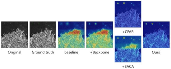
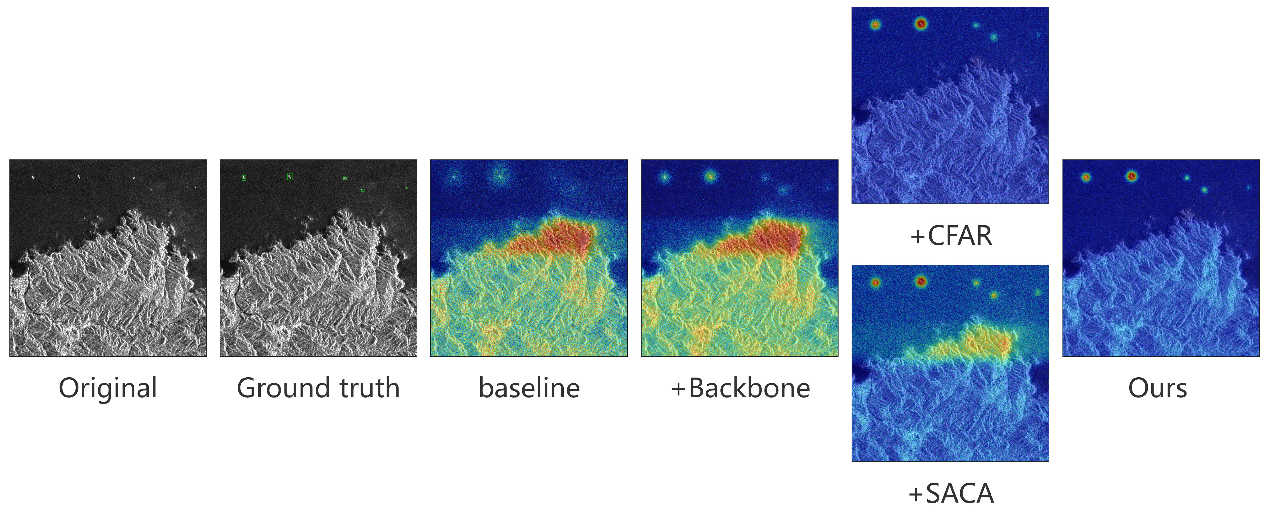
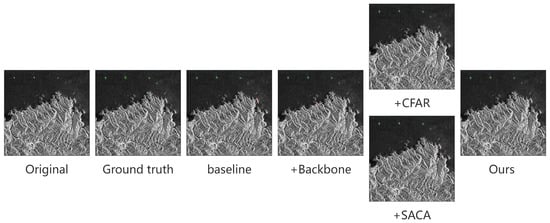
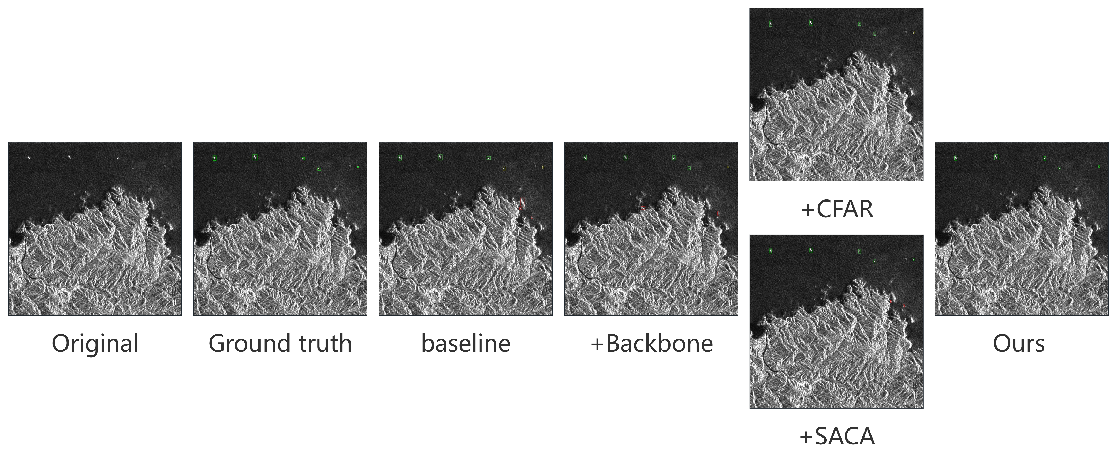
(7) Qualitative evidence. Figure 7 and Figure 8 show feature activation heatmaps and detection results for the ablation configurations. They are examples only, and the conclusions rest on the numbers above.

Figure 7. Stride-8 feature heatmaps for five ablation settings of Table 5. Left to right: (1) SAR image, (2) ground truth, (3) baseline, (4) +backbone, (5) +CFAR-Attention without SACA, (6) +SACA without CFAR-Attention, (7) full model. Columns 5 and 6 show each module on its own. The numbers in Table 5 are the quantitative results.

Figure 8. Detections on the same image as Figure 7. Left to right: (1) SAR image, (2) ground truth, (3) baseline, (4) +backbone, (5) +CFAR-Attention, (6) +SACA, (7) full model. Green: true positive; red: false positive; dashed yellow: miss.

3.5. Complexity and Latency

Table 7 reports parameters, FLOPs, and latency at 1024 × 1024 input. Latency is measured for the model forward pass only (batch size 1, FP32, 500 timed iterations after 100 warm-up iterations, median reported), without data loading or post-processing. FLOPs are counted with the PyTorch profiler, which counts one multiply-add as two operations; the number of multiply-accumulate operations is half of the value shown. Latency depends on the GPU and the software stack, and the values should not be compared with numbers measured elsewhere.

Table 7. Parameters, FLOPs, and latency at 1024 × 1024 input on one RTX 5090 D (FP32, batch size 1, median over 500 runs, model forward only). Parameters are trainable parameters of the training graph.

Config	Description	Params (M)	FLOPs (G)	Latency (ms)	FPS
S1a	R50-vd, no modules	42.70	335.48	16.05	62.3
S1d	R50-vd, full model	43.11	346.56	17.46	57.3
E2	R101-vd, no modules	61.64	490.92	20.46	48.9
E4	R101-vd, Inner + CFAR	61.64	490.95	20.88	47.9
E5	R101-vd, full model	62.05	502.01	21.48	46.6

We take real time to mean at least 30 frames per second (FPS), i.e., at most 33 ms per image, the usual video-rate criterion. SAR products have no single latency requirement, and offline scene processing is less demanding. In the forward pass on the RTX 5090 D, both full models are within this budget (ResNet-50-vd: 17.46 ms, 57.3 FPS; ResNet-101-vd: 21.48 ms, 46.6 FPS). The detector needs no non-maximum suppression, so post-processing is a top-300 selection of the decoder queries, which we did not time separately. As an illustration, a $\mathrm{10,000}\times \mathrm{10,000}$-pixel scene cut into $512\times 512$ tiles with 25% overlap gives $26\times 26=676$ tiles, each resized to $1024\times 1024$. The forward pass alone would take about 12 s with the ResNet-50-vd full model and about 15 s with the ResNet-101-vd full model. These numbers exclude image reading, tiling, and merging of results, and were measured in FP32 on a desktop GPU. They do not show real-time operation on onboard or embedded hardware, which we did not test.

The two modules together add 0.41 M parameters, 2.3% FLOPs and 1.0 ms (5.0%) latency with ResNet-101-vd, and 0.41 M parameters, 3.3% FLOPs and 1.4 ms (8.8%) latency with ResNet-50-vd. CFAR-Attention alone changes the latency by 0.4 ms (2.1%). The ResNet-50-vd full model (S1d, 60.47% AP) needs 29% fewer FLOPs and 15% less latency than the ResNet-101-vd baseline (E2, 59.47% AP) and is 1.00 AP better, so the gain from the modules does not come from a larger backbone.

3.6. Operating Point, False Alarms, Border and Neighbouring Targets

Operating point selected on the validation set. The Precision, Recall, and F1 values above are taken from the test-set P-R curve, which may be optimistic and does not correspond to a specific confidence threshold. We selected the confidence threshold that maximises F1 on the validation set (IoU 0.50, at most 100 detections per image, COCO-style greedy matching). The same threshold was applied to the test set (Table 8). The threshold selected on validation data is within 0.01 to 0.05 of the test-set optimum, and the resulting F1 differs from the values in Table 4 and Table 5 by at most 0.07 (for example, E5: 90.12% against 90.10%; E2: 89.63% against 89.56%). At this operating point the modules help by removing false positives, not by raising Recall. From E2 to E5, Precision changes by $+1.40$, Recall by $-0.42$, and false positives fall from 955 to 810 ($-15.2\%$). From S1a to S1d, Precision changes by $+0.93$, Recall by $+0.20$, and false positives fall from 945 to 852 ($-9.8\%$).

Table 8. Operating point with the confidence threshold selected on the validation set, and false alarms on 2244 ship-free images. $th{r}_{val}$: threshold that maximises F1 on the validation set. TP, FP, FN: true positives, false positives, and false negatives on the test set at $th{r}_{val}$ (9245 instances). FPPI: false alarms per ship-free image at the given confidence threshold. S1e is evaluated at 640 input, the others at 1024.

Config	Description	${\mathit{thr}}_{\mathit{val}}$	Prec.	Recall	F1	TP	FP	FPPI@0.3	FPPI@0.5	FPPI@0.7
S1e	R50-vd/640, none	0.54	88.32	87.43	87.87	8083	1069	0.9348	0.2943	0.0249
S1a	R50-vd/1024, none	0.55	89.72	89.20	89.46	8247	945	0.7924	0.1861	0.0104
S1d	R50-vd/1024, full	0.57	90.65	89.40	90.02	8265	852	0.7135	0.1295	0.0085
E2	R101-vd/1024, none	0.54	89.66	89.61	89.63	8284	955	0.8052	0.1926	0.0093
E5	R101-vd/1024, full	0.56	91.06	89.19	90.12	8246	810	0.7293	0.1363	0.0067

False alarms on ship-free images. We also ran each model on 2244 images ($800\times 800$ pixels, resized to the model input) that contain no ship, so any detection above the confidence threshold is a false alarm. Table 8 gives the number of false alarms per image (FPPI) at three confidence thresholds. At a threshold of 0.5, the full models have about 30% lower FPPI than the corresponding baselines (S1a to S1d: 0.186 to 0.130; E2 to E5: 0.193 to 0.136). The reduction is about 10% at a threshold of 0.3. At a threshold of 0.7, the 1024-pixel models produce only 15 to 23 false alarms each, too few to interpret the relative differences. Input size also matters: from 640 to 1024 pixels, the FPPI at 0.5 falls from 0.294 to 0.186 (S1e to S1a). The pixel spacing of the images is not available, so false alarms per square kilometre cannot be reported. We did not train variants that isolate CFAR-Attention for this test, so the reduction cannot be assigned to a single module.

Border targets. The zero-padded window of CFAR-Attention biases the local mean near the feature-map border. We therefore split the test targets by their distance to the image border (in source-image pixels) and measured Recall at $th{r}_{val}$ (Table 9). Border-touching targets (within 2 pixels of the border, i.e., truncated targets) make up 14.80% of the test instances, the band between 2 and 24 pixels 25.21%, and the interior 59.99%. The band is wider than the zone biased by the padding (24 input pixels, about 6 to 12 source pixels for 256 × 256 to 512 × 512 tiles). Border-touching targets are detected less often than interior targets (Recall 1.0 to 2.0 points lower at 1024 input), and the gap is not larger with the modules (E2: 1.98 points; E5: 1.03; S1a: 1.80; S1d: 1.65). Adding the modules changes the Recall of border-touching targets by $+0.30$ (E2 to E5) and $+0.29$ points (S1a to S1d), within the statistical uncertainty of about 0.9 points for 1368 targets. The zero-padding bias does not appear to harm border targets. Input size has a larger effect: Recall of border-touching targets rises from 81.80% at 640 to 86.84% at 1024 pixels (S1e to S1a), against 87.43% to 88.64% for interior targets.

Table 9. Recall at $th{r}_{val}$ for test targets grouped by distance to the image border (IoU 0.50). Distances are in source-image pixels. Number of targets: 1368 (touching, ≤2 px), 2331 (band, 2–24 px), 5546 (interior, >24 px).

Config	Description	Touching	Band	Interior
S1e	R50-vd/640, none	81.80	90.78	87.43
S1a	R50-vd/1024, none	86.84	91.98	88.64
S1d	R50-vd/1024, full	87.13	92.19	88.78
E2	R101-vd/1024, none	87.13	92.24	89.11
E5	R101-vd/1024, full	87.43	91.98	88.46

Neighbouring targets. To check whether close targets are still detected separately, we grouped the test targets by the distance from their centre to the nearest other target in the same image (source-image pixels). Table 10 gives Recall at $th{r}_{val}$ for each group. Of all targets, 44.36% are alone in their image. Recall is 95.3% to 95.6% for these single targets and 78.7% to 80.0% for targets whose nearest neighbour is closer than 15 pixels, a gap of 15.5 to 17.0 points; it rises with distance to 85.1% to 86.4% beyond 60 pixels. Targets in multi-target images are also missed more often when the nearest neighbour is far away (85.1% to 86.4% against 95.3% to 95.6%), so part of the gap comes from the type of scene, such as busy harbours, and not from proximity alone. The modules do not change Recall consistently in any group (S1a to S1d: $+0.64$ for the closest group and $-0.52$ for the farthest; E2 to E5: $+1.10$ and $-0.77$). The closest group has 367 targets, so the standard error of its Recall is about 2 points, and the differences between models are within this range. The model does not remove the loss of Recall for closely spaced ships, and we did not analyse overlapping or touching ships separately.

Table 10. Recall at $th{r}_{val}$ for test targets grouped by the distance from their centre to the nearest other target in the same image (IoU 0.50, source-image pixels). Number of targets: 4101 (single), 367 (<15 px), 675 (15–30 px), 1255 (30–60 px), 2847 (≥60 px).

Config	Description	Single	<15	15–30	30–60	≥60
S1a	R50-vd/1024, none	95.34	79.40	81.58	84.13	85.66
S1d	R50-vd/1024, full	95.58	80.04	82.63	85.25	85.14
E2	R101-vd/1024, none	95.63	78.67	82.55	84.19	86.41
E5	R101-vd/1024, full	95.37	79.77	82.41	83.45	85.64

4. Discussion

4.1. What CFAR-Attention Does in the Feature Domain

CA-CFAR assumes a known clutter distribution, which gives a closed-form threshold for a chosen false-alarm rate. Deep feature responses follow no such distribution, so this guarantee does not carry over.

We measured how far the response statistics of the trained full model (E5) depart from the Gaussian reference. On the first 1000 test images, background cells (cells outside the ground-truth boxes and at least two cells away from them) had a normalised statistic $z=(s-\widehat{\mu })/\widehat{\sigma }$ with kurtosis 5.3 (stride-8) and 5.8 (stride-16), against 3 for a Gaussian, and a skewness of $-0.77$ and $-0.39$. The empirical exceedance rate $P(z>2)$ was 2.60% at stride-8 and 4.44% at stride-16, against 2.28% for a Gaussian (1.14 and 1.95 times), and $P(z>3)$ was 0.54% and 0.74%, against 0.135% (4.0 and 5.5 times). On the 2244 ship-free images the values were similar ($P(z>3)$: 0.44% and 0.93%; kurtosis 6.1 and 5.7). The response is heavy-tailed, so a constant false-alarm rate does not hold, especially at stride-16 and in the tails. We therefore call the module CFAR-inspired.

The local normalisation still improves the separability of targets from background. Across all pixel pairs, the probability that a target cell has a higher value than a background cell (the area under the receiver operating characteristic (ROC) curve) was 0.834 for z at stride-8 against 0.688 for the raw response s, and 0.831 against 0.750 at stride-16. The mean gate weight was 0.651 on target cells and 0.505 on background cells at stride-8 (0.642 and 0.509 at stride-16), which corresponds to a gain of about 1.046 on targets and 1.035 on background, a difference of only about 1%. The module is a mild reweighting, in line with the 0.5 to 0.6 AP gains in Table 5.

A limitation of the design is that the statistics are computed on the feature map and not on the image: at stride-8 and 1024 × 1024 input, the $7\times 7$ window corresponds to $56\times 56$ input pixels, a coarser context than a classical CFAR reference window.

4.2. SACA and Its Dilation Rates

SACA adds $+0.35$ AP on top of Inner-GIoU and CFAR-Attention, the smallest of the three module gains, and the factorial ablation shows a positive effect in every setting. The gain depends on the dilation set: relative to the model without SACA, the five sets tested give between $-0.11$ and $+0.35$ AP, and the default $\{1,2,4,8\}$ is the highest (Table 6). We did not tune the rates further or test whether SACA transfers to other sensors or resolutions.

4.3. Limitations and Future Work

Boxes, sensors, and resolution. The detector uses axis-aligned boxes, which include much background for ships moored at oblique angles; oriented boxes might help. The benchmark combines nine sources with different sensors and resolutions, and we did not analyse them separately. The SACA dilation rates and the CFAR window were set for the 1024-pixel, stride-8 setting, and other ground resolutions may call for different values. The modules use image intensity only; polarimetric and joint-domain features such as GPCP are not used.

Tuning and statistics. The window $w=7$ and the guard $g=3$ were set in preliminary experiments and their sensitivity is not reported here. The floor on the local standard deviation (0.05) and the optimiser settings were not tuned. Almost all experiments are single runs, and two seeds of the full model differ by up to 0.11 on any metric, so differences of about 0.2 AP or less should be treated as indicative. We did not test whether the Inner-GIoU gain comes from robustness to annotation noise.

Data and evaluation. Results come from one merged benchmark and not from the individual public benchmarks. The split was made after tiling, so neighbouring tiles can lie in different partitions; the overlap audit works on image content and cannot detect shifted, rescaled, or flipped overlap. The benchmark has no sea-state, wind, or pixel-spacing information, so we cannot report results by sea state or false alarms per unit area. The ship-free evaluation covers five models and does not separate the contribution of individual modules. Latency was measured for the forward pass on one desktop GPU.

Closely spaced ships. Recall for ships whose nearest neighbour is closer than 15 pixels is about 16 points lower than for isolated ships, and the modules do not change this consistently (Table 10). Overlapping or touching ships were not analysed separately.

Future work. Next steps are to split the data by scene before tiling and to evaluate each source dataset and sea-state subset separately. Further comparisons should include order-statistic CFAR variants, a learnable or scene-adaptive window, oriented boxes, and polarimetric or joint-domain inputs. Closely spaced ships need a dedicated study, and latency should be measured on onboard hardware over the full processing chain.

5. Conclusions

Small SAR ships can be lost at coarse strides, sea clutter causes false alarms, and a one-pixel annotation offset changes the area of a small box by a large fraction. CaSA-DETR adds a CFAR-inspired local gate on the non-encoder features, a four-branch dilated context block on the stride-8 map, and Inner-GIoU.

On this benchmark, every target is smaller than $32\times 32$ pixels. With ResNet-101-vd and 1024 × 1024 input the full model reaches AP 60.75% and F1 90.10%, 3.96 AP above D-FINE at the same input size. Most of the gain over the original baseline comes from the higher input (+2.46 AP), a smaller part from ResNet-101-vd (+0.44 AP), and 1.0 to 1.4 AP from the three modules, at both backbones and both input sizes. Each module helps in every setting of the others (mean gains: CFAR-Attention 0.54, Inner-GIoU 0.44, SACA 0.27 AP), with no negative interaction. The gain of SACA depends on the dilation set (from $-0.11$ to $+0.35$ AP relative to the model without SACA), whereas AP varies by only 0.22 for r between 0.5 and 0.8. Local mean subtraction recovers about a third of the CFAR-Attention gain. The gate is a mild reweighting, not a constant-false-alarm detector. At a threshold chosen on the validation set, false positives fall by 10% to 15%, and on 2244 ship-free images the false-alarm rate at confidence 0.5 falls by about 30%, at a cost (ResNet-101-vd) of 0.66% parameters, 2.3% FLOPs, and 5% latency.

The main limits are single-run experiments, an overlap check that can miss shifted or flipped tiles, ship-free tests that do not isolate each module, and lower Recall for ships closer than 15 pixels to another ship. Directions for further work are listed in Section 4.3.

References

- Li, J.; Xu, C.; Su, H.; Gao, L.; Wang, T. Deep Learning for SAR Ship Detection: Past, Present and Future. Remote Sens. 2022, 14, 2712. [Google Scholar] [CrossRef] [Scilit]
- Alexandre, C.; Devillers, R.; Mouillot, D.; Seguin, R.; Catry, T. Ship Detection with SAR C-Band Satellite Images: A Systematic Review. IEEE J. Sel. Top. Appl. Earth Obs. Remote Sens. 2024, 17, 14353–14367. [Google Scholar] [CrossRef] [Scilit]
- Lin, T.Y.; Goyal, P.; Girshick, R.; He, K.; Dollár, P. Focal Loss for Dense Object Detection. In Proceedings of the IEEE International Conference on Computer Vision (ICCV); IEEE: New York, NY, USA, 2017; pp. 2980–2988. [Google Scholar] [CrossRef] [Scilit]
- Liu, W.; Anguelov, D.; Erhan, D.; Szegedy, C.; Reed, S.; Fu, C.Y.; Berg, A.C. SSD: Single Shot MultiBox Detector. In Proceedings of the European Conference on Computer Vision (ECCV); Springer: Cham, Switzerland, 2016; pp. 21–37. [Google Scholar] [CrossRef] [Scilit]
- Ren, S.; He, K.; Girshick, R.; Sun, J. Faster R-CNN: Towards Real-Time Object Detection with Region Proposal Networks. In Proceedings of the Advances in Neural Information Processing Systems; NeurIPS: San Diego, CA, USA, 2015; Volume 28, pp. 91–99. [Google Scholar]
- Guo, Y.; Zhan, R.; Chen, S.; Li, L.; Zhang, J. A Lightweight SAR Ship Detection Method Based on Improved YOLOv8. In Proceedings of the IET Conference Proceedings; IET: Stevenage, UK, 2024. [Google Scholar] [CrossRef] [Scilit]
- Khanam, R.; Hussain, M. YOLOv11: An Overview of the Key Architectural Enhancements. arXiv 2024, arXiv:2410.17725. [Google Scholar] [CrossRef] [Scilit]
- Peng, Y.; Li, H.; Wu, P.; Zhang, Y.; Sun, X.; Wu, F. D-FINE: Redefine Regression Task in DETRs as Fine-grained Distribution Refinement. In Proceedings of the International Conference on Learning Representations (ICLR); ICLR: Appleton, WI, USA, 2025. [Google Scholar]
- Tian, Y.; Ye, Q.; Doermann, D. YOLOv12: Attention-Centric Real-Time Object Detectors. arXiv 2025, arXiv:2502.12524. [Google Scholar]
- Chen, S.; Sun, P.; Song, Y.; Luo, P. DiffusionDet: Diffusion Model for Object Detection. In Proceedings of the IEEE/CVF International Conference on Computer Vision (ICCV); IEEE: New York, NY, USA, 2023; pp. 19830–19843. [Google Scholar] [CrossRef] [Scilit]
- Zhou, J.; Xiao, C.; Peng, B.; Liu, Z.; Liu, L.; Liu, Y.; Li, X. DiffDet4SAR: Diffusion-Based Aircraft Target Detection Network for SAR Images. IEEE Geosci. Remote Sens. Lett. 2024, 21, 4007905. [Google Scholar] [CrossRef] [Scilit]
- Carion, N.; Massa, F.; Synnaert, G.; Usunier, N.; Kirillov, A.; Zagoruyko, S. End-to-End Object Detection with Transformers. In Proceedings of the European Conference on Computer Vision (ECCV); Springer: Cham, Switzerland, 2020; pp. 213–229. [Google Scholar] [CrossRef] [Scilit]
- Zhu, X.; Su, W.; Lu, L.; Li, B.; Wang, X.; Dai, J. Deformable DETR: Deformable Transformers for End-to-End Object Detection. In Proceedings of the International Conference on Learning Representations (ICLR); ICLR: Appleton, WI, USA, 2021. [Google Scholar] [CrossRef] [Scilit]
- Zhang, H.; Li, F.; Liu, S.; Zhang, L.; Su, H.; Zhu, J.; Ni, L.M.; Shum, H.Y. DINO: DETR with Improved DeNoising Anchor Boxes for End-to-End Object Detection. In Proceedings of the International Conference on Learning Representations (ICLR); ICLR: Appleton, WI, USA, 2023. [Google Scholar] [CrossRef] [Scilit]
- Zhao, Y.; Lv, W.; Xu, S.; Wei, J.; Wang, G.; Dang, Q.; Liu, Y.; Chen, J. DETRs Beat YOLOs on Real-time Object Detection. In Proceedings of the IEEE/CVF Conference on Computer Vision and Pattern Recognition (CVPR); IEEE: New York, NY, USA, 2024; pp. 16965–16974. [Google Scholar] [CrossRef] [Scilit]
- Zhao, Y.; Lv, W.; Xu, S.; Wei, J.; Wang, G.; Dang, Q.; Liu, Y.; Chen, J. RT-DETRv2: Improved Baseline with Bag-of-Freebies for Real-Time Detection Transformer. arXiv 2024, arXiv:2407.17140. [Google Scholar] [CrossRef] [Scilit]
- Li, C.; Yue, C.; Li, H.; Wang, Z. Context-Aware SAR Image Ship Detection and Recognition Network. Front. Neurorobotics 2024, 18, 1293992. [Google Scholar] [CrossRef] [Scilit] [PubMed]
- Wang, J.; Xu, C.; Yang, W.; Yu, L. A Normalized Gaussian Wasserstein Distance for Tiny Object Detection. arXiv 2021, arXiv:2110.13389. [Google Scholar] [CrossRef] [Scilit]
- El-Darymli, K.; McGuire, P.; Power, D.; Moloney, C. Target Detection in Synthetic Aperture Radar Imagery: A State-of-the-Art Survey. J. Appl. Remote Sens. 2013, 7, 071598. [Google Scholar] [CrossRef] [Scilit]
- Zeng, T.; Zhang, T.; Shao, Z.; Xu, X.; Zhang, W.; Shi, J.; Wei, S.; Zhang, X. CFAR-DP-FW: A CFAR-Guided Dual-Polarization Fusion Framework for Large-Scene SAR Ship Detection. IEEE J. Sel. Top. Appl. Earth Obs. Remote Sens. 2024, 17, 7242–7259. [Google Scholar] [CrossRef] [Scilit]
- Ke, H.; Ke, X.; Zhang, Z.; Chen, X.; Xu, X.; Zhang, T. SLA-Net: A Novel Sea–Land Aware Network for Accurate SAR Ship Detection Guided by Hierarchical Attention Mechanism. Remote Sens. 2025, 17, 3576. [Google Scholar] [CrossRef] [Scilit]
- Hu, J.; Shen, L.; Sun, G. Squeeze-and-Excitation Networks. In Proceedings of the IEEE Conference on Computer Vision and Pattern Recognition (CVPR); IEEE: New York, NY, USA, 2018; pp. 7132–7141. [Google Scholar] [CrossRef] [Scilit]
- Woo, S.; Park, J.; Lee, J.Y.; Kweon, I.S. CBAM: Convolutional Block Attention Module. In Proceedings of the European Conference on Computer Vision (ECCV); Springer: Cham, Switzerland, 2018; pp. 3–19. [Google Scholar] [CrossRef] [Scilit]
- Li, H.; Chen, S.W. General Polarimetric Correlation Pattern: A Visualization and Characterization Tool for Target Joint-Domain Scattering Mechanisms Investigation. IEEE Trans. Geosci. Remote Sens. 2025, 64, 5200417. [Google Scholar] [CrossRef] [Scilit]
- Li, H.; Hu, Y.S.; Chen, S.W. SMEN: Scattering Mechanism Embedded Network for Polarimetric Radar Corner Reflector Array Identification. IEEE Trans. Aerosp. Electron. Syst. 2026, 62, 16728–16744. [Google Scholar] [CrossRef] [Scilit]
- Zhang, H.; Xu, C.; Zheng, S. Inner-IoU: More Effective Intersection over Union Loss with Auxiliary Bounding Box. arXiv 2023, arXiv:2311.02877. [Google Scholar] [CrossRef] [Scilit]
- Wei, S.; Zeng, X.; Qu, Q.; Wang, M.; Su, H.; Shi, J. HRSID: A High-Resolution SAR Images Dataset for Ship Detection and Instance Segmentation. IEEE Access 2020, 8, 120234–120254. [Google Scholar] [CrossRef] [Scilit]
- Zhang, T.; Zhang, X.; Li, J.; Xu, X.; Wang, B.; Zhan, X.; Xu, Y.; Ke, X.; Zeng, T.; Su, H.; et al. SAR Ship Detection Dataset (SSDD): Official Release and Comprehensive Data Analysis. Remote Sens. 2021, 13, 3690. [Google Scholar] [CrossRef] [Scilit]
- Lei, S.; Lu, D.; Qiu, X.; Ding, C. SRSDD-v1.0: A High-Resolution SAR Rotation Ship Detection Dataset. Remote Sens. 2021, 13, 5104. [Google Scholar] [CrossRef] [Scilit]
- Sun, X.; Wang, Z.; Sun, Y.; Diao, W.; Zhang, Y.; Fu, K. AIR-SARShip-1.0: A High-Resolution SAR Dataset for Ship Detection. J. Radars 2019, 8, 852–862. [Google Scholar] [CrossRef]
- Chen, J.; Huang, Z.; Xia, R.; Wu, B.; Sheng, L.; Sun, L.; Yao, B. Large-Scale Multi-Class SAR Image Target Detection Dataset (MSAR-1.0). J. Radars 2022. Available online: https://radars.ac.cn/web/data/getData?dataType=MSAR (accessed on 10 September 2026).
- Xu, C.; Su, H.; Li, J.; Liu, Y.; Zhan, X.; Shi, J. RSDD-SAR: Rotated Ship Detection Dataset in SAR Images. J. Radars 2022, 11, 581–599. [Google Scholar] [CrossRef]
- Hou, X.; Ao, W.; Song, Q.; Lai, J.; Wang, H.; Xu, F. FUSAR-Ship: Building a High-Resolution SAR-AIS Matchup Dataset of Gaofen-3 for Ship Detection and Recognition. Sci. China Inf. Sci. 2020, 63, 140303. [Google Scholar] [CrossRef] [Scilit]
- Wang, Y.; Wang, C.; Zhang, H.; Dong, Y.; Wei, S. A SAR Dataset of Ship Detection for Deep Learning under Complex Backgrounds. Remote Sens. 2019, 11, 765. [Google Scholar] [CrossRef] [Scilit]
- Huang, L.; Liu, B.; Li, B.; Guo, W.; Yu, W.; Zhang, Z.; Yu, W. OpenSARShip: A Dataset Dedicated to Sentinel-1 Ship Interpretation. IEEE J. Sel. Top. Appl. Earth Obs. Remote Sens. 2018, 11, 195–208. [Google Scholar] [CrossRef] [Scilit]
- Pan, Z.; Liu, L.; Qiu, X.; Lei, B. Fast Vessel Detection in Gaofen-3 SAR Images with Ultrafine Strip-Map Mode. Sensors 2017, 17, 1578. [Google Scholar] [CrossRef] [Scilit] [PubMed]
- Chen, L.C.; Papandreou, G.; Schroff, F.; Adam, H. Rethinking Atrous Convolution for Semantic Image Segmentation (DeepLab v3). arXiv 2017, arXiv:1706.05587. [Google Scholar] [CrossRef] [Scilit]
- Rezatofighi, H.; Tsoi, N.; Gwak, J.; Sadeghian, A.; Reid, I.; Savarese, S. Generalized Intersection Over Union: A Metric and a Loss for Bounding Box Regression. In Proceedings of the IEEE/CVF Conference on Computer Vision and Pattern Recognition (CVPR); IEEE: New York, NY, USA, 2019; pp. 658–666. [Google Scholar] [CrossRef] [Scilit]
- Loshchilov, I.; Hutter, F. Decoupled Weight Decay Regularization. In Proceedings of the International Conference on Learning Representations (ICLR); ICLR: Appleton, WI, USA, 2019. [Google Scholar] [CrossRef] [Scilit]
Disclaimer/Publisher’s Note: The statements, opinions and data contained in all publications are solely those of the individual author(s) and contributor(s) and not of MDPI and/or the editor(s). MDPI and/or the editor(s) disclaim responsibility for any injury to people or property resulting from any ideas, methods, instructions or products referred to in the content. |
© 2026 by the authors. Licensee MDPI, Basel, Switzerland. This article is an open access article distributed under the terms and conditions of the Creative Commons Attribution (CC BY) license.