


Highlights
What are the main findings?
- A machine learning-based XCH4 retrieval method integrating TROPOMI spectra, multi-source data, and GOSAT L2 XCH4 correction was developed for China in 2021.
- The retrieved XCH4 captured the spatial variation in methane concentrations over China and showed better consistency with TCCON observations than TROPOMI L2 (R = 0.84).
What are the implications of the main findings?
- Data-driven methods can identify satellite spectral channels important for methane retrieval models and extract key spectral information for regional XCH4 retrieval.
- The east–west gradient of XCH4 over China reveals regional differences driven by climate, surface conditions, and emission characteristics, supporting methane monitoring and source–sink analysis.
Abstract
Methane is a major greenhouse gas that plays a critical role in climate change. Accurate monitoring of methane at the regional scale is essential for understanding its spatiotemporal dynamics and underlying processes. Here, a machine learning-based framework is developed to retrieve column-averaged methane (XCH4) by integrating shortwave infrared spectral information from TROPOMI. Spectral channels are first analyzed through machine learning-based feature importance analysis, and normalized spectral features are subsequently constructed. These features are then combined with auxiliary variables, including meteorological conditions, observation geometry, and surface environmental factors, to develop an XCH4 retrieval model. The GOSAT L2 XCH4 product is introduced as a high-accuracy reference observation for correcting the retrieved XCH4 results, and independent validation is conducted using observations from the TCCON site. Among the evaluated models, XGBoost demonstrates the best performance, achieving an R2 of 0.91 and an RMSE of 9.28 ppb under five-fold cross-validation. The model also maintains relatively better predictive performance compared with other models under both temporal and spatial extrapolation scenarios. Compared with the TROPOMI L2 product, the retrieved XCH4 shows improved agreement with TCCON observations, with a higher correlation (R = 0.84) and reduced errors. Based on this approach, a daily, spatially continuous XCH4 dataset over China for 2021 is generated. Analysis of the retrieved dataset reveals pronounced spatiotemporal patterns, characterized by higher XCH4 concentrations in eastern China and lower values in the western regions, as well as a distinct seasonal cycle.
1. Introduction
Methane is the second most important anthropogenic greenhouse gas after carbon dioxide and plays a critical role in the global climate system [1]. Although its atmospheric concentration is much lower than that of carbon dioxide, methane exhibits a substantially stronger warming effect per unit mass, making a significant contribution to global warming [2]. Previous studies have estimated that methane emissions account for approximately 20% of total radiative forcing. In addition, methane has a relatively short atmospheric lifetime of about 10 years, allowing variations in emissions to exert more rapid impacts on the climate system [3]. Compared with carbon dioxide, which is more challenging to regulate over long timescales, methane mitigation through accurate monitoring and emission control is considered an effective strategy for short-term climate mitigation and for supporting carbon neutrality goals [4,5,6,7]. China is one of the largest methane-emitting countries, characterized by diverse and complex emission sources, including biogenic emissions from rice paddies, wetlands, and livestock, as well as anthropogenic emissions from coal mining, oil and gas production, and landfills [8,9]. Furthermore, China exhibits substantial variability in topography and climate conditions. Atmospheric transport and dispersion processes therefore vary considerably across regions, resulting in pronounced spatial and temporal heterogeneity in XCH4. In this context, obtaining XCH4 data with high spatiotemporal resolution, strong spatial continuity, and high consistency is essential for characterizing regional methane distributions, identifying emission hotspots, and supporting greenhouse gas mitigation policies.
In recent years, ground-based observations and satellite remote sensing have become the primary approaches for monitoring atmospheric methane concentrations. Ground-based measurements provide high accuracy; however, their limited spatial coverage and uneven distribution restrict their ability to support continuous monitoring at regional and national scales [10,11]. In contrast, satellite remote sensing offers extensive spatial coverage, high observation frequency, and strong spatial consistency, effectively overcoming the limitations of ground-based observations. Satellite observations provide XCH4 data, which serve as a fundamental basis for analyzing methane distributions at regional scales [12]. The shortwave infrared (SWIR) spectral band is highly sensitive to near-surface methane and is therefore well suited for capturing its spatial patterns and temporal variability. Consequently, most greenhouse gas monitoring satellites rely on SWIR observations for methane retrieval [13]. Satellite missions such as GOSAT and TROPOMI have played key roles in methane monitoring at both regional and global scales. GOSAT products are characterized by high retrieval accuracy and long-term stability, whereas TROPOMI offers clear advantages for regional applications due to its higher spatial resolution and shorter revisit time [14,15]. Nevertheless, differences in sensor characteristics, retrieval algorithms, and observation conditions introduce unavoidable systematic biases in satellite-derived XCH4 products at the regional scale [16,17].
From the perspective of retrieval methodologies, current atmospheric methane remote sensing predominantly relies on physical inversion approaches [18]. These methods aim to establish physically based relationships between observed spectral signals and atmospheric processes to quantitatively estimate methane concentrations or emissions. For example, Chen et al. [19] combined TROPOMI observations with the GEOS-Chem model to quantify total methane emissions and their sectoral contributions over China. Varon et al. [20] implemented the GEOS-Chem model on a cloud computing platform to reduce computational costs, while Schneising et al. [21] improved the WFM-DOAS algorithm by introducing higher-order polynomials in spectral fitting and integrating machine learning classification to mitigate systematic biases arising from forward model simplifications and instrumental errors. Although these physically based approaches can effectively represent atmospheric radiative transfer processes and achieve high retrieval accuracy, they typically involve numerous physical parameters and iterative calculations, leading to high computational complexity and limited efficiency. This restricts their applicability in large-scale data processing and operational implementations [22,23].
With the rapid growth of hyperspectral remote sensing data and advances in computational capabilities, machine learning methods have been increasingly adopted in methane retrieval studies. These approaches estimate XCH4 by learning statistical relationships between remote sensing features and methane concentrations, offering improved computational efficiency. Wan et al. [24] used GOSAT XCH4 data and meteorological variables to estimate surface methane concentrations with an XGBoost model. Masiello et al. [25] trained a feed-forward neural network using simulated IASI spectral radiances to retrieve atmospheric methane profiles, while Jin et al. [26] combined TROPOMI XCH4 data with meteorological, topographic, and other auxiliary variables using a Random Forest model to reconstruct areas with missing satellite observations. These studies demonstrate the potential of machine learning for satellite-based methane retrieval and estimation. Regarding the combined use of multi-source satellite observations, Qu et al. [27] compared methane observations from TROPOMI and GOSAT. GOSAT showed a mean bias of −1.0 ppb and a regional bias metric of 2.9 ppb, compared with −2.7 ppb and 6.7 ppb, respectively, for TROPOMI, indicating differences in the systematic biases and their spatial variations between the two products. Balasus et al. [28] further used collocated GOSAT and TROPOMI observations to estimate and correct retrieval biases in the TROPOMI methane product using machine learning. Li et al. [29] used GOSAT XCH4 as the training target and combined it with TROPOMI spectral radiance data to retrieve global methane concentrations. These studies provide a basis for combining complementary GOSAT and TROPOMI observations to improve methane retrieval and correct product biases.
Building on the above considerations, this study focuses on China and uses the TROPOMI L2 XCH4 product as the initial training target. SHAP-based feature importance analysis is used to construct normalized difference spectral features, which are combined with meteorological variables, viewing geometry, and surface environmental variables to establish a machine learning-based retrieval model. The GOSAT XCH4 product is then used to correct the model retrieval results, and the final product is validated against ground-based TCCON observations. Based on the validated retrievals, the spatiotemporal distribution of XCH4 across China is further analyzed.
2. Study Area and Data Sources
2.1. Study Area
This study focuses on China, covering approximately 3°N–54°N and 73°E–135°E. The region encompasses a wide range of terrain and climate zones, extending from the Tibetan Plateau to the eastern coastal areas. It includes diverse climate regimes, ranging from cold temperate to subtropical zones, and exhibits substantial regional variability in climate conditions, land cover, and human activity intensity. Topographically, the study area is characterized by a pronounced west–east gradient, with higher elevations in the west and lower elevations in the east. The western region is dominated by the Tibetan Plateau and surrounding mountainous areas, where elevations are generally high and can exceed 4000 m. In contrast, the central region mainly consists of hills and basins, while the eastern region is characterized by extensive plains and coastal lowlands, accompanied by high population density and intensive human activities. Such complex terrain and heterogeneous human influences contribute to pronounced spatial variability in atmospheric methane across China.
Figure 1 illustrates the geographic location and topographic distribution of the study area. Elevation is represented by color, clearly highlighting the decreasing terrain from west to east. The two TCCON sites used for validation of the retrieval results are also indicated, including the Xianghe site (39.8°N, 116.96°E) located in the North China Plain and the Hefei site (31.9°N, 117.17°E) located in eastern China.
Figure 1.
Study area. The background colors indicate topographic elevation (m), and the inset in the lower-right corner shows the South China Sea Islands.
2.2. TROPOMI Satellite Data
TROPOMI is a tropospheric atmospheric composition monitoring instrument onboard the ESA Sentinel-5P satellite, launched in October 2017. The instrument covers the ultraviolet, visible, near-infrared, and shortwave infrared spectral bands, providing global observations of atmospheric composition [30]. Since August 2019, the spatial resolution of its shortwave infrared (SWIR) band has been approximately 7 km × 5.5 km, an improvement over the initial resolution of approximately 7 km × 7 km. This improvement enables more detailed characterization of the spatial distribution of atmospheric methane column concentrations at regional scales, making TROPOMI an important data source for regional methane monitoring.
In this study, both the TROPOMI L2 XCH4 product and L1B spectral radiance data are utilized. The L2 XCH4 product is retrieved by the Institute of Environmental Physics, University of Bremen, using the WFM-DOAS algorithm [21,31]. Based on SWIR observations, this product provides XCH4 data with high retrieval accuracy and long-term stability and has been widely applied in both regional and global methane studies.
The TROPOMI L1B product provides radiometrically calibrated hyperspectral measurements together with detailed observation geometry information. The instrument covers the ultraviolet, visible, near-infrared, and shortwave infrared spectral ranges, comprising eight independent spectral bands, each corresponding to a separate L1B product. In addition to spectral radiance, the L1B data include key observation geometry parameters, such as solar zenith angle (SZA), solar azimuth angle (SAA), viewing zenith angle (VZA), and viewing azimuth angle (VAA). This study primarily uses SWIR Band 7 (2305–2345 nm) data from 2021, which captures the main methane absorption features. These data, together with the corresponding observation geometry parameters, provide the basis for subsequent XCH4 retrieval and analysis. In addition, only high-quality TROPOMI data with qa_value > 0.5 were retained.
2.3. GOSAT XCH4 Product
GOSAT is the first satellite dedicated to global greenhouse gas monitoring and is equipped with the Thermal And Near-infrared Sensor for carbon Observation–Fourier Transform Spectrometer (TANSO-FTS). This instrument provides high-resolution spectral observations in both the shortwave infrared and thermal infrared bands, enabling the retrieval of column-averaged greenhouse gas concentrations, including XCH4 [32,33].
The GOSAT L2 XCH4 product is characterized by high retrieval accuracy and long-term stability and has been widely used for cross-validation of satellite methane products, background concentration estimation, and trend analysis [27,34,35]. Although its spatial resolution is relatively coarse, its high accuracy makes it a reliable reference for evaluating the consistency of regional methane retrievals.
2.4. TCCON Observations
The Total Carbon Column Observing Network (TCCON) is a global network of ground-based observation sites established in 2004. It employs high-resolution Fourier transform infrared (FTIR) spectrometers to record solar absorption spectra in the near-infrared region after sunlight passes through the atmosphere. These spectra are used to retrieve column-averaged concentrations of greenhouse gases, including carbon dioxide, methane, and carbon monoxide. The resulting data are highly accurate and stable over long periods and are widely used as reference measurements for validating satellite-based greenhouse gas retrieval products [36,37].
The Xianghe site (39.8°N, 116.96°E), located in the central part of the North China Plain, is characterized by intensive industrial activities and high population density. It represents the atmospheric composition characteristics of typical human-affected regions in eastern China [38]. The Hefei site (31.9°N, 117.17°E), located in the middle and lower reaches of the Yangtze River region in Anhui Province, has different surface conditions and regional atmospheric backgrounds compared with the North China Plain. In this study, TCCON observations from both sites in 2021 are used to validate the satellite retrieval results, and daily averages are calculated from the original measurements.
2.5. ERA5 Reanalysis Data
Considering the differences in atmospheric conditions, topography, and surface radiation environments across regions, Wan et al. [24] and Jin et al. [26] incorporated auxiliary features such as meteorological variables, surface elevation, and solar radiation into satellite-based methane concentration estimation to complement spectral observations. Schneising et al. [31] also considered the effects of solar zenith angle, viewing angle, surface elevation, and atmospheric temperature on radiative transfer and retrieval results in their study of the TROPOMI methane retrieval algorithm. Based on these studies, meteorological variables and surface environmental data are incorporated into the model as auxiliary inputs.
ERA5 is the fifth-generation global atmospheric reanalysis dataset produced by the European Centre for Medium-Range Weather Forecasts (ECMWF) and released in 2017. It provides continuous data from 1950 to the present, with an hourly temporal resolution and a wide range of atmospheric, land, and oceanic variables. The dataset has a spatial resolution of approximately 30 km and represents the atmosphere using 137 vertical levels from the surface up to 80 km [39].
In this study, several ERA5 variables are used, including boundary layer height (BLH), total precipitation (TP), 10 m u and v wind components (U10 and V10), 2 m temperature (T2M), total column water vapor (TCWV), surface net solar radiation (SNSR), and relative humidity (RH). All variables are aggregated to daily averages and resampled to a spatial resolution of 0.05° × 0.05°.
2.6. Surface Environmental Data
2.6.1. DEM
The digital elevation model (DEM) is a digital representation of surface elevation, typically organized as a regular grid in which each cell records the elevation at a specific location. It can be used to characterize terrain relief and surface morphology [40]. Topographic conditions can influence atmospheric structure and near-surface gas dispersion, thereby affecting the spatial distribution of atmospheric methane. Elevation data obtained from Google Earth are used to characterize terrain differences and assess their potential impact on methane column concentrations.
2.6.2. Downward Shortwave Radiation Data
Downward shortwave radiation (DSR) plays a key role in surface energy balance, vegetation activity, and evapotranspiration and can indirectly influence methane emissions and atmospheric processes. In this study, the DSR TOPO product from the GLASS dataset is used, with a spatial resolution of 0.05° [41,42]. This product is derived from MODIS observations combined with topographic information and provides reliable estimates of surface incoming shortwave radiation.
2.6.3. Vegetation Index
Vegetation conditions are represented by the normalized difference vegetation index (NDVI). NDVI data are obtained from the MOD13C1 Level 3 product provided by the Moderate Resolution Imaging Spectroradiometer (MODIS) onboard the Terra satellite [43]. The dataset has a spatial resolution of 0.05° and a temporal resolution of 16 days and is used to characterize vegetation conditions and their potential relationship with biogenic methane emissions.
2.7. Cloud Mask Data
To minimize the impact of clouds on shortwave infrared methane observations, the Level-2 cloud mask product CLDMSK_L2_VIIRS_SNPP released by NASA is used. This product is derived from observations of the Visible Infrared Imaging Radiometer Suite (VIIRS) onboard the Suomi National Polar-orbiting Partnership (SNPP) satellite. It is based on the MODIS–VIIRS cloud mask (M-VCM) algorithm framework and determines cloud conditions and their confidence levels using multispectral threshold tests [44].
3. Methodology
This study presents a high-resolution XCH4 retrieval framework over China by integrating multi-source remote sensing data with machine learning techniques, with the overall workflow illustrated in Figure 2. TROPOMI SWIR spectral data serve as the primary input, together with observation geometry parameters, ERA5 reanalysis data, and surface environmental variables. Spectral channels are first selected through feature importance analysis, and normalized spectral features are constructed to enhance methane-related signals. These features are then combined with auxiliary data to build the retrieval model. To improve consistency, we further incorporate the GOSAT L2 XCH4 product as a reference dataset. The model is subsequently evaluated using TCCON observations, and the validated results are used to analyze the spatial distribution of XCH4 over China.
Figure 2.
Overview of the proposed framework for XCH4 retrieval and analysis.
3.1. Normalized Spectral Index Construction
Following the spectral channel importance analysis, the 10 channels with the highest SHAP importance scores and the 10 channels with the lowest scores are selected as high- and low-importance channels, respectively. The radiance values of these two groups are then used to construct normalized difference spectral features.
The normalized spectral index is defined as:
In the equation, represents the radiance of a high-importance channel, while represents the radiance of its corresponding low-importance channel.
The rationale for constructing these features is based on the physical principle of differential spectroscopy, which uses relative radiance differences between nearby spectral bands to reduce the influence of common background effects. Within the SWIR region, spectrally close channels may be similarly affected by surface reflectance and viewing conditions. Calculating the difference between channel radiances and normalizing it can help characterize the relative radiance differences between channels. Following this approach, the selected high- and low-importance channels are sorted by central wavelength and paired one-to-one to construct normalized difference spectral features. The resulting normalized difference spectral features, together with meteorological variables, surface auxiliary data, and viewing geometry parameters, form the input feature set for the retrieval model.
3.2. Methane Retrieval Models
To capture the nonlinear relationships between multi-source remote sensing features and XCH4, several tree-based machine learning models are employed, including XGBoost, Random Forest, LightGBM, and Extra Trees. These models are well suited for handling high-dimensional data, nonlinear relationships, and complex feature interactions and have been widely applied in remote sensing retrieval studies.
3.2.1. XGBoost
XGBoost is an ensemble learning algorithm based on gradient boosting decision trees, proposed by Chen and Guestrin [45]. It improves prediction accuracy by iteratively fitting the residuals from previous models. For the i-th sample, the prediction can be expressed as the sum of outputs from multiple regression trees:
where is the input feature vector, denotes the k-th regression tree, and represents the space of regression tree functions. This structure enables the model to capture complex nonlinear relationships between input features and the target variable.
During training, XGBoost optimizes model parameters by minimizing an objective function with a regularization term. The overall objective function is defined as:
where is the loss function that measures the difference between predicted and true values, and is the regularization term that controls model complexity. The regularization term is defined as:
where T is the number of leaf nodes in a regression tree, is the weight of the j-th leaf node, γ and λ are regularization parameters that control tree complexity and leaf weights, respectively. By incorporating this regularization term, XGBoost effectively balances model complexity and fitting accuracy, thereby reducing overfitting and improving generalization performance.
3.2.2. Random Forest
Random Forest is a machine learning method based on ensemble learning. Its theoretical foundation can be traced back to the random subspace method proposed by Ho in 1995 [46]. Breiman further developed and formalized the Random Forest algorithm in 2001 [47] by combining bootstrap resampling with random feature selection. This design improves model stability and generalization, making Random Forest a widely used ensemble learning approach. The core idea is to build multiple independent decision trees and aggregate their predictions to improve overall model performance, as illustrated in Figure 3. During training, the method generates multiple subsets by sampling the original data with replacement. At each split in a decision tree, it randomly selects a subset of features for node partitioning, which reduces the model’s dependence on specific features or samples.
Figure 3.
Random Forest flowchart.
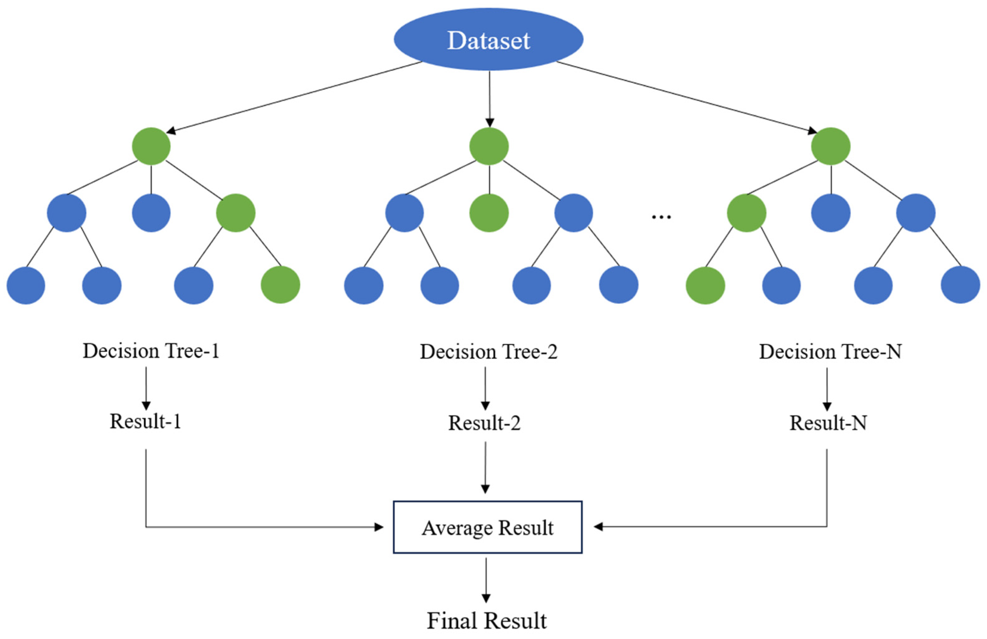
By introducing randomness in both samples and features, Random Forest effectively reduces overfitting compared to a single decision tree and shows strong robustness to noisy data. In addition, the model does not rely on strict assumptions about data distribution and is insensitive to the scale of input features, making it well suited for high-dimensional and multi-source remote sensing data.
3.2.3. LightGBM
LightGBM is an efficient gradient boosting decision tree algorithm proposed by Ke et al. [48] in 2017. It represents an important improvement over traditional gradient boosting decision tree (GBDT) methods. Similar to standard GBDT, LightGBM adopts an additive model structure and iteratively fits the residuals from previous iterations. It combines multiple regression trees to predict the target variable. During training, LightGBM minimizes a loss function. The objective function can be written as:
where l(⋅) is the loss function, typically the squared loss in regression tasks. Unlike XGBoost, LightGBM does not explicitly introduce complex regularization terms. Instead, it controls model complexity through algorithm design and sampling strategies.
To address the high computational cost and memory consumption of traditional GBDT under large sample sizes and high-dimensional features, LightGBM introduces two key techniques: Gradient-based One-Side Sampling (GOSS) and Exclusive Feature Bundling (EFB) [48]. GOSS retains samples with large gradient values and randomly samples those with small gradients, reducing the number of training samples while maintaining the accuracy of split gain estimation. EFB exploits the sparsity of high-dimensional feature space by bundling mutually exclusive features, which effectively reduces feature dimensionality and computational cost.
In addition, LightGBM uses a histogram-based feature discretization method to map continuous features into discrete bins, reducing the complexity of split point search. It also adopts a leaf-wise tree growth strategy and achieves lower training error under the same depth constraint. As a result, LightGBM improves training efficiency while maintaining high prediction accuracy.
3.2.4. Extra Trees
Extra Trees is an ensemble decision tree method proposed by Geurts et al. [49] in 2006. It follows a similar framework to Random Forest by combining multiple decision trees but introduces stronger randomness during tree construction. The increased randomness reduces the correlation between trees, improves generalization performance, and increases training efficiency.
During training, Extra Trees not only randomly selects candidate features at each split but also generates random split thresholds for each feature. It then selects the best split from these randomly generated candidates [50]. Unlike Random Forest, Extra Trees does not search for the optimal split point among candidate features. Instead, it randomizes the split thresholds, significantly reducing the computational cost of split search and improving efficiency for high-dimensional features and large datasets. Increased randomness in the splitting process leads to greater diversity among trees, reduces ensemble variance, and improves prediction stability. Extra randomness may introduce some bias. However, averaging the outputs of a large number of randomized trees allows the model to achieve a good balance between bias and variance.
3.3. GOSAT-Based Correction of XCH4 Retrieval Results
Due to differences in spatial resolution, sampling strategies, observation geometries, and retrieval algorithms among satellite sensors, XCH4 products from different satellite missions generally exhibit certain systematic discrepancies. TROPOMI provides continuous regional-scale methane column observations with relatively high spatial coverage; however, its retrieval results may still be affected by surface reflectance characteristics, atmospheric state parameters, and retrieval priors. The GOSAT XCH4 product, benefiting from its relatively high retrieval accuracy and stable observation capability, provides an independent reference for the optimization of regional-scale XCH4 products.
Considering the sparse spatial coverage of GOSAT observations, which limits their ability to independently support the continuous generation of regional methane column concentration products at high spatial resolution, this study uses the TROPOMI L2 XCH4 product as the supervised training target for the first stage model. TROPOMI L1B spectral features and multi-source auxiliary variables are combined to establish an initial XCH4 retrieval model. The GOSAT L2 XCH4 product is then used to correct the initial retrieval results. Specifically, the initial XCH4 retrievals are matched spatiotemporally with corresponding GOSAT L2 observations to construct training samples for the correction model. The initial retrieval results serve as the primary input, together with spectral features, meteorological variables, surface environmental parameters, and viewing geometry information. The machine learning model then learns the nonlinear relationships between these variables and the matched GOSAT XCH4 observations to correct biases in the initial retrieval product.
The correction stage uses the best performing model selected through the first stage model comparison, with matched GOSAT XCH4 observations serving as the reference for establishing a mapping between the initial retrieval results and the reference observations. The trained correction model is subsequently applied to the initial retrieval product to generate the final XCH4 product. Both the initial and corrected products are validated against ground-based TCCON observations to evaluate the effects of the correction procedure on retrieval performance.
4. Results
4.1. Spectral Channel Importance Analysis for Methane
TROPOMI Band 7 contains 480 continuous spectral channels covering the primary methane absorption features. However, using all channels in the retrieval introduces substantial redundancy and multicollinearity, which can reduce model stability and computational efficiency. Meanwhile, the contributions of individual channels to me-thane retrieval vary considerably. Therefore, spectral channel selection is necessary to reduce the dimensionality of the spectral data and provide a basis for subsequent spectral feature construction.
First, a candidate spectral range was defined according to methane absorption features in the SWIR region to establish the initial spectral feature set. SHAP analysis then quantified the relative contribution of each spectral channel to model predictions. Ranking the channels by their mean absolute SHAP values identified the top 10 as high-importance channels and the bottom 10 as low-importance channels (Table 1).
Table 1.
Spectral channel selection results based on SHAP feature importance rankings.
4.2. Effect of Spectral Feature Construction on XCH4 Retrieval
To evaluate the constructed normalized spectral features, three comparative experiments were conducted to examine the effects of different spectral input configurations on XCH4 retrieval performance while keeping the training samples and auxiliary variables unchanged. Model 1 used the raw radiance values of the top 10 high-importance channels, whereas Model 2 incorporated the raw radiance values of both the high- and low-importance channels. Model 3 employed normalized difference spectral features constructed from the high- and low-importance channels. The evaluation metrics of the three configurations were compared to determine the spectral input representation for subsequent modeling. By comparing the evaluation metrics across the three configurations, the most suitable spectral input representation was selected for subsequent modeling.
As shown in Table 2, the model achieves good retrieval performance using only the raw radiance values of the high-importance channels, with an R2 of 0.906 and an RMSE of 9.436 ppb. This result suggests that the SHAP-selected high-importance channels effectively capture spectral information related to methane absorption. However, adding the raw radiance values of the low-importance channels does not further improve performance; instead, R2 decreases slightly to 0.904, and RMSE increases to 9.491 ppb. In contrast, the normalized difference spectral features constructed from the high- and low-importance channels yield the best results, with R2 increasing to 0.909 and MAE and RMSE decreasing to 6.477 ppb and 9.281 ppb, respectively. Although the performance differences among the three configurations are relatively small, Model 3 demonstrates a modest advantage. Therefore, subsequent experiments use the spectral input configuration of Model 3 and further investigate the contributions of different types of auxiliary variables through grouped ablation experiments.
Table 2.
Comparison of XCH4 retrieval performance using different spectral input configurations.
4.3. Model Comparison
The retrieval experiments are conducted using data from the entire year of 2021, covering diverse seasonal and regional conditions. Under five-fold cross-validation, all models capture the nonlinear relationships between multi-source remote sensing features and XCH4. XGBoost achieves the best overall performance, with R2 = 0.909, RMSE = 9.281 ppb, and MAE = 6.477 ppb. Moreover, the bias remains close to zero, indicating strong fitting ability and effective control of systematic errors (Figure 4a). Random Forest achieves similar performance, with R2 = 0.906 and RMSE = 9.432 ppb. Its bias shows a slightly larger magnitude, indicating slightly lower stability compared to XGBoost (Figure 4b). The scatter points from both models align closely with the 1:1 line and form dense clusters without obvious systematic deviation, indicating comparable fitting performance. In contrast, LightGBM and Extra Trees exhibit lower retrieval accuracy (Figure 4c,d). Their R2 values decrease to 0.891 and 0.882, respectively, with RMSE values exceeding 10 ppb and higher MAE values. This indicates a relatively weaker ability to capture XCH4 variability under the current feature set and data conditions.
Figure 4.
Scatter plots of five-fold cross-validation results for (a) XGBoost; (b) Random Forest; (c) LightGBM; (d) Extra Trees. (The blue line represents the fitted regression line, and the red line represents the line of equality y = x).
XCH4 retrieval models often face temporal distribution shifts and strong spatial heterogeneity in practical applications, which cannot be fully captured by standard cross-validation under identical data distributions. To better assess model generalization, two additional validation strategies are introduced: temporal extrapolation and spatial extrapolation. Temporal extrapolation adopts a leave-one-season-out strategy, in which data from three seasons are used for training and the remaining season for testing. This setup evaluates model stability and adaptability under seasonal transitions. Spatial extrapolation is implemented using a spatial block cross-validation approach, where the study area is divided into 2° × 2° grids. In each iteration, approximately 30% of the blocks are used for testing, while the remaining blocks are used for training. This strategy assesses model transferability across spatially independent regions.
Under five-fold cross-validation, XGBoost and Random Forest exhibit comparable performance and achieve the highest overall accuracy among all models. Further evaluation focuses on these two models using temporal and spatial extrapolation tests. As shown in Table 3, both models maintain moderate correlations across all seasons under the leave-one-season-out setting. However, XGBoost consistently outperforms Random Forest, with higher correlation coefficients and lower MAE and RMSE values in most seasons, indicating improved stability and error control. Although both models exhibit seasonal systematic biases, the magnitude of bias is generally smaller for XGBoost. Under spatial extrapolation (Table 4), both models show reduced accuracy compared with same-distribution validation, reflecting the increased difficulty of spatial generalization. Nevertheless, XGBoost maintains higher correlation and lower errors than Random Forest, while the bias for both models remains close to zero, suggesting no evident spatial systematic bias.
Table 3.
Comparison of temporal extrapolation results across different seasons.
Table 4.
Comparison of spatial extrapolation results.
Overall, although XGBoost and Random Forest perform similarly under the same distribution conditions, XGBoost demonstrates superior stability and generalization capability under both temporal and spatial distribution shifts. It is therefore selected as the optimal model for subsequent retrieval.
4.4. Effects of Different Auxiliary Variable Groups on Retrieval Performance
After determining the normalized difference spectral features, we further examined the effects of different auxiliary variable groups on XCH4 retrieval performance. Using the full-feature model as the baseline, three ablation experiments were conducted by removing the viewing geometry parameters (SAA, SZA, VAA, and VZA), meteorological variables (BLH, RH, SNSR, TCWV, TP, U10, V10, and T2M), and surface environmental variables (DSR, DEM, and NDVI), respectively, while keeping the remaining features unchanged.
The auxiliary variable ablation results in Table 5 demonstrate that the full model achieves the best retrieval performance. Among the three auxiliary variable groups, viewing geometry parameters have the greatest impact on model performance. Removing these parameters reduces R2 to 0.878 and increases MAE and RMSE to 7.568 ppb and 10.736 ppb, respectively. Removing meteorological variables also leads to a noticeable decline in performance, with R2 decreasing to 0.888 and RMSE increasing to 10.286 ppb. In comparison, surface environmental variables have a smaller but still positive contribution, as their removal reduces R2 to 0.902 and increases RMSE to 9.647 ppb. Overall, these results highlight the importance of viewing geometry and meteorological variables in XCH4 retrieval, while surface environmental variables provide additional useful information. Therefore, subsequent analyses retain the full feature set and use SHAP to further examine the relative importance of individual variables.
Table 5.
Comparison of XCH4 retrieval performance in the auxiliary variable ablation experiments.
4.5. SHAP Interpretable Analysis
To better understand the retrieval mechanism of XCH4, SHAP analysis evaluates the importance of input variables and their contributions to model predictions. SHAP originates from the concept of Shapley values in game theory and was originally developed to measure the contribution of individual players to the overall payoff. In model interpretation, it quantifies the contribution of each input feature to the prediction [51,52].
Figure 5 shows the feature importance ranking and the contribution distribution of input variables. Spectral features dominate the model, with Spec_9, T2M, SAA, Spec_6, VAA, and Spec_8 exhibiting the highest mean absolute SHAP values. Variables associated with observation geometry and surface conditions contribute at a moderate level, whereas meteorological variables such as wind speed and precipitation exhibit SHAP values clustered near zero, indicating a limited influence on the retrieval. In terms of contribution direction, higher values of T2M, SAA, VAA, DEM, Spec_10, and Spec_1 generally increase the predicted XCH4, indicating positive contributions. In contrast, Spec_9, Spec_6, Spec_8, VZA, DSR, and NDVI show negative contributions. These results suggest that the model primarily relies on spectral information, while temperature and observation geometry play secondary but important roles. The relative importance of variables remains clearly distinguishable, highlighting the interpretability of the model.
Figure 5.
Importance ranking and contribution distribution of input variables.
Figure 6 further illustrates the SHAP dependence relationships for key variables, using color mapping to reveal interaction effects that influence XCH4 retrieval. Spectral variables exhibit a generally stable negative relationship with SHAP values, with clear transitions near zero-contribution thresholds. For a given feature value, variations in TCWV or neighboring spectral channels lead to stratified SHAP patterns, indicating strong interaction effects among variables. Among meteorological variables, T2M shows an approximately linear positive relationship with SHAP values, with stronger effects at higher temperatures, particularly under the modulation of spectral features such as Spec_2. This suggests a synergistic interaction between temperature and spectral information. In contrast, TCWV exhibits a nonlinear response, with rapid increases at low values followed by saturation, indicating higher sensitivity under dry atmospheric conditions. The observation geometry parameters exhibit pronounced nonlinear behavior. The relationship between VAA and SHAP values may also be influenced by observations at large viewing azimuth angles. In this study, observations with |VAA| > 60° were not excluded, and these data may include measurements from adjacent orbits overlapping with the primary orbit, with different observation times from those of the primary orbit. In addition, large viewing angles may increase uncertainties in the retrieved XCH4 values. Future studies could exclude observations with |VAA| > 60° to reduce the potential influence of these factors. For surface and environmental variables, DEM shows a consistent positive relationship, whereas DSR exerts a negative influence at higher values and varies with temperature, suggesting interactions between surface radiation and thermal conditions.
Figure 6.
SHAP dependence plots of key variables. The colors of the scatter points represent the values of the corresponding interacting features. The light pink shading indicates feature values below the SHAP = 0 threshold, while the light blue shading indicates values above it. The annotated values indicate the feature values at which the SHAP dependence curves cross zero.
4.6. Validation with TCCON Observations
4.6.1. Validation of Retrieval Results
For site scale validation, regional means within a ±2° spatial window around each TCCON station were extracted and temporally matched on a daily basis, ensuring a consistent benchmark across all evaluated products. Figure 7 presents the scatter plots comparing the TROPOMI L2 product, the uncorrected model retrievals, the directly corrected TROPOMI L2 product, and the final corrected product against TCCON observations. The directly corrected TROPOMI L2 product was obtained by using the original TROPOMI L2 product as the product to be corrected and training a correction model with matched GOSAT XCH4 observations. In contrast, the final corrected product was generated using the two-stage retrieval framework proposed in this study. Specifically, preliminary retrievals were first performed using TROPOMI L1B spectral features and multi-source auxiliary variables, after which the preliminary retrieval results were further corrected using GOSAT observations. The main difference between the two approaches lies in the input product used during the correction stage: the former directly corrects the original TROPOMI L2 product, whereas the latter applies a further correction to the retrieval results obtained in the first stage. The original TROPOMI L2 product yielded a correlation coefficient of 0.756, an RMSE of 15.70 ppb, and an MAE of 12.06 ppb (Figure 7a). The uncorrected model retrieval achieved a correlation coefficient of 0.781 and reduced the RMSE to 15.02 ppb (Figure 7b). The directly corrected L2 product yielded a correlation coefficient of 0.777 and an RMSE of 15.45 ppb (Figure 7c). In contrast, the final corrected product achieved a correlation coefficient of 0.839, with the RMSE and MAE decreasing to 13.89 ppb and 10.84 ppb, respectively (Figure 7d). Compared with the original L2 product, the final corrected product reduced the RMSE and MAE by approximately 11.6% and 10.1%, respectively, and achieved a higher correlation with TCCON observations. It also achieved a higher correlation coefficient and lower RMSE and MAE than the directly corrected L2 product, indicating better overall agreement with ground-based observations. However, the final corrected product still exhibited a negative bias of −5.27 ppb, whose absolute magnitude was greater than that of the original L2 product (−2.38 ppb). In addition, all four products had regression slopes below 1, and most samples at the high concentration end fell below the 1:1 reference line. This pattern indicates that the retrieved XCH4 values vary less than the TCCON observations as concentrations increase, suggesting an underestimation of high XCH4 concentrations. Therefore, although the final corrected product improves correlation and overall error metrics, its bias and response to high-concentration variations still warrant further investigation.
Figure 7.
Comparison of four XCH4 products with TCCON observations: (a) original TROPOMI L2 product; (b) uncorrected model retrievals; (c) directly corrected TROPOMI L2 product; and (d) final corrected product. (The blue line represents the regression line, and the red line represents the 1:1 line).
4.6.2. Time Series Comparison
Figure 8 presents the comparison of daily XCH4 time series between the retrieved results and TCCON observations at the two validation sites. For the Xianghe site (Figure 8a), the retrieval results show good consistency with the TCCON observations in terms of the overall annual variation, with both datasets exhibiting a gradual increase from relatively low values at the beginning of the year and reaching higher levels in late summer and early autumn. In contrast, the time series at the Hefei site (Figure 8b) is relatively more scattered due to the limited number of available observations. Nevertheless, the retrieval results still capture the overall variation pattern of the TCCON observations, with both datasets showing a clear increasing trend from mid-year to autumn. This pattern reflects a clear seasonal cycle of methane concentration at the regional scale.
Figure 8.
Comparison of daily XCH4 time series between TCCON observations and model retrieval results at (a) Xianghe and (b) Hefei sites.
At shorter time scales, the retrieval exhibits reduced variability compared with TCCON observations and fails to fully capture certain high-concentration events, leading to an underestimation of extreme values, particularly in late summer and early autumn. This discrepancy can be attributed to differences in spatial representativeness, as satellite retrievals reflect spatial averages, whereas TCCON observations are more sensitive to local and short-term concentration enhancements. Furthermore, the number of valid observations at Hefei Station is relatively limited, which may also increase the uncertainty of the daily average results. Despite these limitations, the retrieval remains consistent with TCCON observations in terms of temporal trends, seasonal phase, and long-term variability, supporting its applicability for regional-scale methane monitoring and time series analysis.
4.7. Spatiotemporal Distribution of XCH4 in China
4.7.1. Spatial Distribution and Comparison with the TROPOMI L2 Product
Following XCH4 retrieval and correction, a machine learning model was used to spatially reconstruct the results, generating a daily, spatially complete gridded XCH4 product over China at a spatial resolution of 0.05°. The resulting product was then used to analyze the spatial distribution and spatiotemporal variations in XCH4 and to compare the results with the TROPOMI L2 XCH4 product. The retrieved XCH4 distribution (Figure 9a) shows a clear east–west spatial gradient, characterized by relatively lower values in western China and higher values in central and eastern China. Lower XCH4 concentrations are mainly observed over the Tibetan Plateau, the arid regions of northwestern China, and high-altitude areas, whereas relatively elevated XCH4 levels are found over the North China Plain, the middle and lower reaches of the Yangtze River, and southern China. The longitudinal profile (Figure 9c) further demonstrates that XCH4 generally increases with increasing longitude. The concentration rises rapidly east of approximately 100°E and reaches relatively high levels around 110.2°E, followed by a slight decrease toward eastern China while remaining at elevated levels. Particularly, the transition region from the Tibetan Plateau to the eastern plains exhibits an enhanced spatial gradient in both the distribution pattern and the longitudinal variation curve. The Sichuan Basin presents a local high-value region at the annual scale, contrasting with its surrounding areas. In comparison, most regions of northeastern and northwestern China remain at intermediate XCH4 levels.
Figure 9.
Annual mean spatial distribution of XCH4 over China in 2021 and comparison between the model-retrieved results and the TROPOMI L2 product: (a) spatial distribution of model-retrieved XCH4; (b) spatial distribution of TROPOMI L2 XCH4; (c) longitudinal variation in zonal-mean XCH4; and (d) spatial difference between the model-retrieved results and the TROPOMI L2 product (Model − TROPOMI L2).
The TROPOMI L2 XCH4 product (Figure 9b) also exhibits a pronounced east–west gradient, and its high- and low-concentration regions generally agree well with those identified by the model retrievals. Both datasets show similar spatial patterns over the Tibetan Plateau, northwestern China, and the high-concentration regions in central and eastern China. However, the difference map (Figure 9d) indicates that the discrepancies between the retrieved XCH4 and TROPOMI L2 vary spatially and do not exhibit a consistent systematic bias. Most regions show differences close to zero. Negative biases are mainly distributed over parts of central-western and northern China, represented by blue areas, indicating that the retrieved XCH4 values are slightly lower than those from the TROPOMI L2 product. In contrast, positive biases are more frequently observed in central and eastern China, particularly over the Sichuan Basin, central China, and parts of eastern China, where the retrieved values are relatively higher than the TROPOMI L2 observations. In addition, localized positive biases are also found in northeastern and northern China, but with relatively limited spatial extent and magnitude.
The monthly mean XCH4 concentrations and seasonal spatial difference distributions of the two products are shown in Figure 10. In terms of monthly means (Figure 10a), the differences between the two products remained small from January to June, with absolute differences below 4 ppb. Starting in July, the model results became lower than the TROPOMI L2 values, and the difference gradually increased, reaching a maximum of −14.31 ppb in August. The difference then narrowed, although the model results remained approximately 7 ppb lower than the L2 product at the end of the year. The seasonal difference maps reveal clear regional variations in the discrepancies between the two products, which also change with season. In spring, negative differences dominate most of central and western China, whereas positive differences appear in the northeast and parts of central and eastern China (Figure 10b). In summer, negative differences are mainly distributed across southwestern and south-central China, while more pronounced positive differences occur in the northeast (Figure 10c). In autumn, negative differences are widespread across western, central, and parts of northern China, while localized positive differences persist in the northeast (Figure 10d). In winter, the spatial contrasts become more pronounced, with negative differences prevailing in northern and northwestern China and more evident positive differences across southern and southwestern China (Figure 10e).
Figure 10.
Monthly variations and seasonal spatial differences between model-retrieved XCH4 and the TROPOMI L2 product over China in 2021. (a) Monthly mean XCH4 concentrations from the two products; (b) spring, (c) summer, (d) autumn, and (e) winter spatial differences between the model retrievals and the TROPOMI L2 product (Model − TROPOMI L2).
To further examine seasonal variations, Figure 11 presents the spatial distribution of XCH4 across spring, summer, autumn, and winter. While the overall spatial pattern remains consistent with the annual mean, notable differences are observed in both spatial extent and intensity. In spring, relatively high concentrations are evident in central and eastern China, whereas the Tibetan Plateau and its surrounding areas maintain lower levels, resulting in pronounced regional contrasts. In summer, XCH4 concentrations increase across most of China, and high-concentration areas expand, particularly in eastern and southern China, where the spatial distribution becomes more continuous. The autumn pattern is similar to that in summer, but high-concentration areas become more concentrated in central and eastern China. In winter, XCH4 concentrations decline noticeably in western China and the plateau regions, while eastern China maintains relatively high levels, further accentuating the east–west contrast. These seasonal differences may be associated with seasonal variations in methane emissions and changes in temperature, precipitation, and atmospheric transport conditions. Meteorological conditions and emission activities jointly influence the regional distribution of XCH4, resulting in distinct spatial patterns across seasons.
Figure 11.
Seasonal distribution of XCH4 over China in 2021: (a) spring; (b) summer; (c) autumn; (d) winter.
4.7.2. Temporal Variation Characteristics
Figure 12 presents the monthly variation in the national mean XCH4 in 2021, together with the corresponding monthly maximum, minimum, and spatial standard deviation. The national mean XCH4 exhibits a clear intra-annual variation pattern. The mean value reaches 1865.38 ppb in January and slightly decreases to 1862.80 ppb in February, marking the lowest level of the year. From March onward, XCH4 increases gradually, with a more pronounced rise after June, and peaks at 1903.56 ppb in August, approximately 40 ppb higher than the February minimum. Thereafter, it declines progressively toward the end of the year. Overall, XCH4 exhibits a single-peak seasonal pattern, characterized by elevated concentrations in summer and lower levels in winter. The monthly maximum and minimum values follow trends consistent with the mean, indicating coherent variability across different statistical metrics. Spatial variability also shows pronounced seasonal dependence. The spatial standard deviation decreases significantly during summer, reaching a minimum of approximately 14 ppb in July and August, whereas it increases during winter and early spring, exceeding 26 ppb at its maximum. This seasonal contrast suggests that methane concentrations become more spatially homogeneous during summer, likely due to widespread emission enhancement and stronger atmospheric mixing. In contrast, winter is characterized by enhanced spatial heterogeneity, with larger differences between eastern and western regions. This pattern can be attributed to the combined effects of reduced biological emissions, regionally variable anthropogenic sources, and weaker atmospheric mixing, which together amplify regional contrasts in XCH4.
Figure 12.
Monthly mean variation in XCH4 over China in 2021.
To further investigate regional differences, Figure 13 compares monthly XCH4 variations across provinces in eastern, central, western, and northeastern China. Across all regions, XCH4 exhibits a consistent seasonal cycle, increasing from winter and spring, peaking in late summer to early autumn, and subsequently declining. Eastern China maintains the highest overall XCH4 levels, with provinces such as Jiangsu, Shanghai, and Guangdong showing pronounced summer and autumn peaks (Figure 13a). This pattern reflects the combined influence of dense population, intensive energy consumption, and strong agricultural activity. In central China, temporal variations are relatively stable, although Shanxi exhibits slightly lower concentrations and reduced variability (Figure 13b). Western China shows the strongest spatial heterogeneity, with substantial differences among provinces (Figure 13c). Sichuan, Chongqing, and Shaanxi maintain relatively high XCH4 levels, whereas Qinghai and Tibet remain at much lower levels. In Tibet, XCH4 stays low during winter and spring, increases rapidly in summer, and peaks around August, indicating a large seasonal amplitude. This variation may be associated with seasonal temperature changes at high elevations and atmospheric transport conditions. The Sichuan Basin and its surrounding areas may be affected by factors such as regional emissions, topography and atmospheric dispersion conditions, maintaining relatively high concentration levels. In northeastern China, XCH4 remains at moderate levels, with Liaoning, Jilin, and Heilongjiang showing similar temporal patterns and moderate seasonal variability (Figure 13d).
Figure 13.
Monthly variation in XCH4 across provinces in different regions of China: (a) eastern China; (b) central China; (c) western China; (d) northeastern China.
5. Discussion
Existing studies of XCH4 over China have mainly focused on analyzing spatiotemporal distributions using existing satellite products, ground-based observations, or derived datasets [53,54,55]. Ground-based observations provide high accuracy, but the limited number of stations makes it difficult to fully characterize spatial variations at the regional scale. Satellite products offer broader spatial coverage, but observation conditions can prevent them from consistently providing continuous gridded data. In this study, machine learning-based retrieval and spatial reconstruction were used to generate a daily XCH4 product over China at a spatial resolution of 0.05°, providing a basis for analyzing concentration gradients and seasonal variations across the country. Comparison with the TROPOMI L2 product also reveals broadly similar spatial distributions and intra-annual variation patterns, although differences remain across regions and time periods.
TCCON validation further indicates that the overall retrieval accuracy has improved, with the correlation coefficient increasing from 0.756 to 0.839, the RMSE decreasing from 15.701 to 13.886 ppb, and the MAE decreasing from 12.056 to 10.842 ppb. However, these overall metrics do not fully capture model performance under different concentration conditions. To examine this performance in greater detail, the matched samples were sorted in ascending order according to the XCH4 concentrations observed by TCCON and divided into four equal-sized groups, referred to as quartiles (Q1–Q4). Q1 represents the lowest-concentration quartile, whereas Q4 represents the highest-concentration quartile. The validation results for the four concentration groups are summarized in Table 6. The RMSE of the retrieved product in Q1, Q2, and Q3 was 10.614, 9.518, and 11.772 ppb, respectively, all lower than that of the original L2 product. However, in Q4, the RMSE increased from 19.953 ppb for the original L2 product to 20.724 ppb for the retrieved product, while the bias changed from −10.551 to −16.947 ppb. Meanwhile, the bias of the retrieved product shifted from a positive value of 5.690 ppb in Q1 to negative values in Q2, Q3, and Q4, with increasingly pronounced negative bias at higher concentrations. These results indicate that although the model improves overall retrieval accuracy, it remains less effective at estimating high XCH4 concentrations. Consequently, overall evaluation metrics alone cannot fully reflect retrieval performance across different concentration ranges.
Table 6.
Validation results for the TROPOMI L2 and corrected XCH4 products across different TCCON concentration groups.
This underestimation of high concentrations also needs to be considered in subsequent spatiotemporal analyses. Because the bias varies across concentration ranges, underestimation of high XCH4 values may reduce the apparent concentration contrast between local hotspots and their surrounding areas, affecting the assessment of regional concentration gradients and hotspot intensity. At the temporal scale, if high concentrations occur mainly in certain months or seasons, this bias may also suppress the corresponding peaks, causing the actual magnitude of concentration variations to be underestimated. Therefore, the spatial patterns and seasonal trends identified in this study remain informative, but quantitative assessments of concentrations in high-value regions, local extremes, and seasonal amplitudes should not rely solely on the retrieval results. In particular, when comparing concentration differences between regions or seasons, the validation results should also be considered to distinguish actual concentration variations from potential effects of model errors.
These limitations are partly related to the data-driven nature of the retrieval approach. Machine learning models primarily learn statistical relationships between input features and XCH4 concentrations from training samples, without explicitly incorporating physical constraints associated with atmospheric transport and other processes. As a result, they may not fully capture complex variations under high-concentration conditions [28,56]. Future research could improve the representation of high-concentration samples and incorporate independent observations and atmospheric chemical transport models to constrain and validate retrievals under these conditions. In addition, radiative transfer simulations could support a more physically grounded analysis of spectral sensitivity by quantitatively assessing how changes in methane concentration, surface reflectance, water vapor content, and viewing geometry affect the radiance responses of different spectral channels. Building on these improvements, sustained retrievals using multi-year satellite observations could extend the study period and expand the geographical coverage, ultimately producing XCH4 datasets with broader spatial coverage and longer time series to support a more comprehensive analysis of long-term methane variations and regional differences.
6. Conclusions
This study develops an XCH4 retrieval framework for China by integrating TROPOMI shortwave infrared spectral information, machine learning methods, and multi-source auxiliary data. The framework generates spatially continuous XCH4 distribution data over China for 2021. The main conclusions are as follows:
- (1)
- Feature importance analysis of TROPOMI SWIR spectral channels identifies channels with high importance to model predictions, and normalized spectral features are constructed by combining high- and low-importance channels. Comparative experiments show that the normalized difference spectral features yield a modest improvement in retrieval performance compared with using the raw radiance values of the top 10 channels ranked by importance.
- (2)
- By integrating spectral features, observation geometry parameters, meteorological reanalysis data, and surface environmental variables, multiple tree-based models are developed for XCH4 retrieval. Among them, XGBoost achieves the best performance, with R2 = 0.91, RMSE = 9.28 ppb, and MAE = 6.48 ppb under five-fold cross-validation. Moreover, compared with the Random Forest model, XGBoost achieves higher correlation coefficients and lower error levels under both temporal and spatial extrapolation tests, indicating its better overall retrieval performance under the current study area and validation conditions.
- (3)
- Compared with the original TROPOMI L2 product, the final corrected product shows improved agreement with the combined TCCON observations from the Xianghe and Hefei sites. The correlation coefficient increases from 0.76 to 0.84, while the RMSE and MAE decrease from 15.70 ppb to 13.89 ppb and from 12.06 ppb to 10.84 ppb, respectively. The time series comparison further confirms that the retrieval effectively captures intra-annual variability and seasonal patterns, although some underestimation of short-term extreme values remains. At the regional scale over China, the retrieved results showed a consistent spatial distribution pattern with the TROPOMI L2 product. The differences between the two datasets were generally small, with no apparent overall positive or negative bias. Negative biases were mainly observed in western China and parts of northern China, whereas positive biases were found in some regions of central and eastern China.
- (4)
- The retrieved XCH4 dataset reveals pronounced spatiotemporal variability across China. A clear east–west gradient is observed, with XCH4 concentrations generally increasing with longitude, showing elevated values in eastern China and lower values in the west. High-value regions are mainly distributed in the North China Plain, the middle and lower reaches of the Yangtze River, and southern China, whereas the Tibetan Plateau and its surrounding areas form prominent low-value regions. This spatial pattern may be associated with the combined effects of regional emission activities, ecological conditions, and meteorological factors. At the temporal scale, XCH4 exhibits a well-defined seasonal cycle, with minimum levels in winter and early spring and a gradual increase toward summer, peaking in late summer, indicating the combined effects of emission intensity and seasonal atmospheric processes.
Overall, the proposed framework provides an effective approach for generating high-resolution and continuous XCH4 data at the regional scale. The resulting dataset offers a valuable basis for investigating methane spatiotemporal variability over China. Future work could incorporate additional high-concentration samples and independent observations and integrate atmospheric chemical transport models or radiative transfer simulations to impose physical constraints on the retrieval results, thereby enhancing the framework’s potential for methane emission attribution and process-oriented analysis.
Author Contributions
Conceptualization, M.J. and L.T.; methodology, M.J.; software, M.J.; validation, M.J.; formal analysis, M.J.; investigation, M.J. and L.T.; resources, L.T.; data curation, M.J.; writing—original draft preparation, M.J.; writing—review and editing, L.T.; visualization, M.J.; supervision, L.T.; project administration, L.T.; funding acquisition, L.T. All authors have read and agreed to the published version of the manuscript.
Funding
This research was funded by the National Natural Science Foundation of China (Grant No. 42371349) and the National Key Research and Development Program of China (Grant No. 2023YFE0100500).
Data Availability Statement
The TROPOMI L1B data used in this study are publicly available from the European Space Agency (https://browser.dataspace.copernicus.eu (accessed on 11 November 2025)). The TROPOMI L2 XCH4 product retrieved by the Institute of Environmental Physics, University of Bremen, using the WFM-DOAS algorithm is available at (https://www.iup.uni-bremen.de/carbon_ghg/products/tropomi_wfmd/ (accessed on 11 November 2025)). The GOSAT XCH4 products can be obtained from the GOSAT Data Archive Service (https://data2.gosat.nies.go.jp (accessed on 25 November 2025)). TCCON observations are available from the TCCON Data Archive (https://tccondata.org (accessed on 10 December 2025)). ERA5 meteorological data can be accessed through the European Centre for Medium-Range Weather Forecasts at (https://cds.climate.copernicus.eu (accessed on 11 May 2026). The NDVI data were obtained from NASA (https://lpdaac.usgs.gov (accessed on 29 November 2025)), and the downward shortwave radiation data are obtained from the GLASS dataset (http://www.glass.umd.edu (accessed on 3 December 2025)). The DEM data are obtained from publicly available global elevation datasets. All data used in this study are publicly available and can be accessed from the above sources.
Acknowledgments
We thank the providers of all the datasets used in the article for making their data publicly accessible. In addition, We acknowledged the Nanjing University of Information Science and Technology for the support of this work.
Conflicts of Interest
The authors declare no conflicts of interest.
References
- Fawzy, S.; Osman, A.I.; Doran, J.; Rooney, D.W. Strategies for mitigation of climate change: A review. Environ. Chem. Lett. 2020, 18, 2069–2094. [Google Scholar] [CrossRef] [Scilit]
- Forster, P.; Storelvmo, T.; Armour, K.; Collins, W.; Dufresne, J.-L.; Frame, D.; Lunt, D.J.; Mauritsen, T.; Palmer, M.D.; Watanabe, M.; et al. The Earth’s Energy Budget, Climate Feedbacks, and Climate Sensitivity. In Climate Change 2021: The Physical Science Basis. Contribution of Working Group I to the Sixth Assessment Report of the Intergovernmental Panel on Climate Change; Chapter 7; Cambridge University Press: Cambridge, UK, 2021; pp. 923–1054. [Google Scholar] [CrossRef] [Scilit]
- Stocker, T.F.; Qin, D.; Plattner, G.K.; Alexander, L.V.; Allen, S.K.; Bindoff, N.L.; Bréon, F.M.; Church, J.A.; Cubasch, U.; Emori, S.; et al. Technical summary. In Climate Change 2013: The Physical Science Basis. Contribution of Working Group I to the Fifth Assessment Report of the Intergovernmental Panel on Climate Change; Cambridge University Press: Cambridge, UK, 2013; pp. 33–115. [Google Scholar]
- Nisbet, E.G.; Manning, M.R.; Dlugokencky, E.J.; Fisher, R.E.; Lowry, D.; Michel, S.E.; Myhre, C.L.; Platt, S.M.; Allen, G.; Bousquet, P.; et al. Very strong atmospheric methane growth in the 4 years 2014–2017: Implications for the Paris Agreement. Glob. Biogeochem. Cycles 2019, 33, 318–342. [Google Scholar] [CrossRef] [Scilit]
- Nisbet, E.G.; Fisher, R.E.; Lowry, D.; France, J.L.; Allen, G.; Bakkaloglu, S.; Broderick, T.J.; Cain, M.; Coleman, M.; Fernandez, J.; et al. Methane mitigation: Methods to reduce emissions, on the path to the Paris Agreement. Rev. Geophys. 2020, 58, e2019RG000675. [Google Scholar] [CrossRef] [Scilit]
- Nisbet, E.G.; Dlugokencky, E.J.; Bousquet, P. Methane on the rise—Again. Science 2014, 343, 493–495. [Google Scholar] [CrossRef] [Scilit] [PubMed]
- Kirschke, S.; Bousquet, P.; Ciais, P.; Saunois, M.; Canadell, J.G.; Dlugokencky, E.J.; Bergamaschi, P.; Bergmann, D.; Blake, D.R.; Bruhwiler, L.; et al. Three decades of global methane sources and sinks. Nat. Geosci. 2013, 6, 813–823. [Google Scholar] [CrossRef] [Scilit]
- Bousquet, P.; Ciais, P.; Miller, J.B.; Dlugokencky, E.J.; Hauglustaine, D.A.; Prigent, C.; Van der Werf, G.R.; Peylin, P.; Brunke, E.G.; Carouge, C.; et al. Contribution of anthropogenic and natural sources to atmospheric methane variability. Nature 2006, 443, 439–443. [Google Scholar] [CrossRef] [Scilit] [PubMed]
- Tian, H.; Lu, C.; Ciais, P.; Michalak, A.M.; Canadell, J.G.; Saikawa, E.; Huntzinger, D.N.; Gurney, K.R.; Sitch, S.; Zhang, B.; et al. The terrestrial biosphere as a net source of greenhouse gases to the atmosphere. Nature 2016, 531, 225–228. [Google Scholar] [CrossRef] [Scilit] [PubMed]
- Sha, M.K.; De Mazière, M.; Notholt, J.; Blumenstock, T.; Chen, H.; Dehn, A.; Griffith, D.W.T.; Hase, F.; Heikkinen, P.; Hermans, C.; et al. Intercomparison of low- and high-resolution infrared spectrometers for ground-based solar remote sensing measurements of total column concentrations of CO2, CH4, and CO. Atmos. Meas. Tech. 2020, 13, 4791–4839. [Google Scholar] [CrossRef] [Scilit]
- Cai, K.; Yang, X.; Li, S.; Xiao, Y.; Qiao, B.; Liu, Y. Accuracy verification of satellite products and temporal and spatial distribution analysis and prediction of the CH4 concentration in China. Remote Sens. 2023, 15, 2813. [Google Scholar] [CrossRef] [Scilit]
- Yoshida, Y.; Ota, Y.; Eguchi, N.; Kikuchi, N.; Nobuta, K.; Tran, H.; Morino, I.; Yokota, T. Retrieval algorithm for CO2 and CH4 column abundances from short-wavelength infrared spectral observations by the Greenhouse gases observing satellite. Atmos. Meas. Tech. 2011, 4, 717–734. [Google Scholar] [CrossRef] [Scilit]
- Jacob, D.J.; Varon, D.J.; Cusworth, D.H.; Dennison, P.E.; Frankenberg, C.; Gautam, R.; Guanter, L.; Kelley, J.; McKeever, J.; Ott, L.E.; et al. Quantifying methane emissions from the global scale down to point sources using satellite observations of atmospheric methane. Atmos. Chem. Phys. 2022, 22, 9617–9646. [Google Scholar] [CrossRef] [Scilit]
- Wecht, K.J.; Jacob, D.J.; Sulprizio, M.P.; Santoni, G.W.; Wofsy, S.C.; Parker, R.; Bösch, H.; Worden, J. Spatially resolving methane emissions in California: Constraints from the CalNex aircraft campaign and from present (GOSAT, TES) and future (TROPOMI, geostationary) satellite observations. Atmos. Chem. Phys. 2014, 14, 8173–8184. [Google Scholar] [CrossRef] [Scilit]
- Lorente, A.; Borsdorff, T.; Butz, A.; Hasekamp, O.; Schneider, A.; Wu, L.; Hase, F.; Kivi, R.; Wunch, D.; Pollard, D.F.; et al. Methane retrieved from TROPOMI: Improvement of the data product and validation of the first 2 years of measurements. Atmos. Meas. Tech. 2021, 14, 665–684. [Google Scholar] [CrossRef] [Scilit]
- Kulawik, S.S.; Worden, J.R.; Payne, V.H.; Fu, D.; Wofsy, S.C.; McKain, K.; Sweeney, C.; Daube, B.C., Jr.; Lipton, A.; Polonsky, I.; et al. Evaluation of single-footprint AIRS CH4 profile retrieval uncertainties using aircraft profile measurements. Atmos. Meas. Tech. 2021, 14, 335–354. [Google Scholar] [CrossRef] [Scilit]
- Xiong, X.; Barnet, C.; Maddy, E.; Sweeney, C.; Liu, X.; Zhou, L.; Goldberg, M. Characterization and validation of methane products from the Atmospheric Infrared Sounder (AIRS). J. Geophys. Res. Biogeosci. 2008, 113, G00A01. [Google Scholar] [CrossRef] [Scilit]
- Parker, R.J.; Webb, A.; Boesch, H.; Somkuti, P.; Barrio Guillo, R.; Di Noia, A.; Kalaitzi, N.; Anand, J.S.; Bergamaschi, P.; Chevallier, F.; et al. A decade of GOSAT Proxy satellite CH4 observations. Earth Syst. Sci. Data 2020, 12, 3383–3412. [Google Scholar] [CrossRef] [Scilit]
- Chen, Z.; Jacob, D.J.; Nesser, H.; Sulprizio, M.P.; Lorente, A.; Varon, D.J.; Lu, X.; Shen, L.; Qu, Z.; Penn, E.; et al. Methane emissions from China: A high-resolution inversion of TROPOMI satellite observations. Atmos. Chem. Phys. 2022, 22, 10809–10826. [Google Scholar] [CrossRef] [Scilit]
- Varon, D.J.; Jacob, D.J.; Sulprizio, M.; Estrada, L.A.; Downs, W.B.; Shen, L.; Hancock, S.E.; Nesser, H.; Qu, Z.; Penn, E.; et al. Integrated Methane Inversion (IMI 1.0): A user-friendly, cloud-based facility for inferring high-resolution methane emissions from TROPOMI satellite observations. Geosci. Model Dev. 2022, 15, 5787–5805. [Google Scholar] [CrossRef] [Scilit]
- Schneising, O.; Buchwitz, M.; Hachmeister, J.; Vanselow, S.; Reuter, M.; Buschmann, M.; Bovensmann, H.; Burrows, J.P. Advances in retrieving XCH4 and XCO from Sentinel-5 Precursor: Improvements in the scientific TROPOMI/WFMD algorithm. Atmos. Meas. Tech. 2023, 16, 669–694. [Google Scholar] [CrossRef] [Scilit]
- Liu, Y.; Wang, J.; Che, K.; Cai, Z.; Yang, D.; Wu, L. Satellite remote sensing of greenhouse gases: Progress and trends. Natl. Remote Sens. Bull. 2021, 25, 53–64. [Google Scholar] [CrossRef] [Scilit]
- Hu, H.; Hasekamp, O.; Butz, A.; Galli, A.; Landgraf, J.; Aan de Brugh, J.; Borsdorff, T.; Scheepmaker, R.; Aben, I. The operational methane retrieval algorithm for TROPOMI. Atmos. Meas. Tech. 2016, 9, 5423–5440. [Google Scholar] [CrossRef] [Scilit]
- Wan, Y.; Chen, F.; Fan, L.; Sun, D.; He, H.; Dai, Y.; Li, L.; Chen, Y. Conversion of surface CH4 concentrations from GOSAT satellite observations using XGBoost algorithm. Atmos. Environ. 2023, 301, 119694. [Google Scholar] [CrossRef] [Scilit]
- Masiello, G.; Mastro, P.; Serio, C.; Falabella, F.; Pasquariello, P. Methane profile retrieval from IASI: A deep learning inversion approach based on feed-forward neural networks. In Remote Sensing of Clouds and the Atmosphere XXVII; SPIE: Breda, The Netherlands, 2022; Volume 12265, pp. 41–49. [Google Scholar] [CrossRef] [Scilit]
- Jin, Z.; He, J.; Wang, W. Monitoring methane concentrations with high spatial resolution over China by using random forest model. Remote Sens. 2024, 16, 2525. [Google Scholar] [CrossRef] [Scilit]
- Qu, Z.; Jacob, D.J.; Shen, L.; Lu, X.; Zhang, Y.; Scarpelli, T.R.; Nesser, H.; Sulprizio, M.P.; Maasakkers, J.D.; Bloom, A.A.; et al. Global distribution of methane emissions: A comparative inverse analysis of observations from the TROPOMI and GOSAT satellite instruments. Atmos. Chem. Phys. 2021, 21, 14159–14175. [Google Scholar] [CrossRef] [Scilit]
- Balasus, N.; Jacob, D.J.; Lorente, A.; Maasakkers, J.D.; Parker, R.J.; Boesch, H.; Chen, Z.; Kelp, M.M.; Nesser, H.; Varon, D.J. A blended TROPOMI+GOSAT satellite data product for atmospheric methane using machine learning to correct retrieval biases. Atmos. Meas. Tech. 2023, 16, 3787–3807. [Google Scholar] [CrossRef] [Scilit]
- Li, K.; Bai, K.; Jiao, P.; Chen, H.; He, H.; Shao, L.; Sun, Y.; Zheng, Z.; Li, R.; Chang, N.-B. Developing unbiased estimation of atmospheric methane via machine learning and multiobjective programming based on TROPOMI and GOSAT data. Remote Sens. Environ. 2024, 304, 114039. [Google Scholar] [CrossRef] [Scilit]
- Veefkind, J.P.; Aben, I.; McMullan, K.; Förster, H.; de Vries, J.; Otter, G.; Claas, J.; Eskes, H.J.; de Haan, J.F.; Kleipool, Q.; et al. TROPOMI on the ESA Sentinel-5 Precursor: A GMES mission for global observations of the atmospheric composition for climate, air quality and ozone layer applications. Remote Sens. Environ. 2012, 120, 70–83. [Google Scholar] [CrossRef] [Scilit]
- Schneising, O.; Buchwitz, M.; Reuter, M.; Bovensmann, H.; Burrows, J.P.; Borsdorff, T.; Deutscher, N.M.; Feist, D.G.; Griffith, D.W.T.; Hase, F.; et al. A scientific algorithm to simultaneously retrieve carbon monoxide and methane from TROPOMI onboard Sentinel-5 Precursor. Atmos. Meas. Tech. 2019, 12, 6771–6802. [Google Scholar] [CrossRef] [Scilit]
- Kuze, A.; Suto, H.; Nakajima, M.; Hamazaki, T. Thermal and near infrared sensor for carbon observation Fourier-transform spectrometer on the Greenhouse Gases Observing Satellite for greenhouse gases monitoring. Appl. Opt. 2009, 48, 6716–6733. [Google Scholar] [CrossRef] [Scilit] [PubMed]
- Suto, H.; Kataoka, F.; Kikuchi, N.; Knuteson, R.O.; Butz, A.; Haun, M.; Buijs, H.; Shiomi, K.; Imai, H. Thermal and near-infrared sensor for carbon observation Fourier transform spectrometer-2 (TANSO-FTS-2) on the Greenhouse gases Observing SATellite-2 (GOSAT-2) during its first year in orbit. Atmos. Meas. Tech. 2021, 14, 2013–2039. [Google Scholar] [CrossRef] [Scilit]
- Someya, Y.; Yoshida, Y.; Ohyama, H.; Nomura, S.; Kamei, A.; Morino, I.; Mukai, H.; Matsunaga, T.; Laughner, J.L.; Velazco, V.A.; et al. Update on the GOSAT TANSO–FTS SWIR Level 2 retrieval algorithm. Atmos. Meas. Tech. 2023, 16, 1477–1501. [Google Scholar] [CrossRef] [Scilit]
- Sheng, J.-X.; Jacob, D.J.; Turner, A.J.; Maasakkers, J.D.; Benmergui, J.; Bloom, A.A.; Arndt, C.; Gautam, R.; Zavala-Araiza, D.; Boesch, H.; et al. 2010–2016 methane trends over Canada, the United States, and Mexico observed by the GOSAT satellite: Contributions from different source sectors. Atmos. Chem. Phys. 2018, 18, 12257–12267. [Google Scholar] [CrossRef] [Scilit]
- Laughner, J.L.; Toon, G.C.; Mendonca, J.; Petri, C.; Roche, S.; Wunch, D.; Blavier, J.F.; Griffith, D.W.; Heikkinen, P.; Keeling, R.F.; et al. The Total Carbon Column Observing Network’s GGG2020 data version. Earth Syst. Sci. Data 2024, 16, 2197–2260. [Google Scholar] [CrossRef] [Scilit]
- Wunch, D.; Toon, G.C.; Blavier, J.F.L.; Washenfelder, R.A.; Notholt, J.; Connor, B.J.; Griffith, D.W.; Sherlock, V.; Wennberg, P.O. The Total Carbon Column Observing Network. Philos. Trans. R. Soc. A Math. Phys. Eng. Sci. 2011, 369, 2087–2112. [Google Scholar] [CrossRef] [Scilit] [PubMed]
- Yang, Y.; Zhou, M.; Langerock, B.; Sha, M.K.; Hermans, C.; Wang, T.; Ji, D.; Vigouroux, C.; Kumps, N.; Wang, G.; et al. New ground-based Fourier-transform near-infrared solar absorption measurements of XCO2, XCH4 and XCO at Xianghe, China. Earth Syst. Sci. Data 2020, 12, 1679–1696. [Google Scholar] [CrossRef] [Scilit]
- Hersbach, H.; Bell, B.; Berrisford, P.; Hirahara, S.; Horányi, A.; Muñoz-Sabater, J.; Nicolas, J.; Peubey, C.; Radu, R.; Schepers, D.; et al. The ERA5 global reanalysis. Q. J. R. Meteorol. Soc. 2020, 146, 1999–2049. [Google Scholar] [CrossRef] [Scilit]
- Guth, P.L.; Van Niekerk, A.; Grohmann, C.H.; Muller, J.P.; Hawker, L.; Florinsky, I.V.; Gesch, D.B.; Reuter, H.I.; Herrera-Cruz, V.; Riazanoff, S.; et al. Digital elevation models: Terminology and definitions. Remote Sens. 2021, 13, 3581. [Google Scholar] [CrossRef] [Scilit]
- Zhang, X.; Wang, D.; Liu, Q.; Yao, Y.; Jia, K.; He, T.; Jiang, B.; Wei, Y.; Ma, H.; Zhao, X.; et al. An operational approach for generating the global land surface downward shortwave radiation product from MODIS data. IEEE Trans. Geosci. Remote Sens. 2019, 57, 4636–4650. [Google Scholar] [CrossRef] [Scilit]
- Liang, S.; Cheng, J.; Jia, K.; Jiang, B.; Liu, Q.; Xiao, Z.; Yao, Y.; Yuan, W.; Zhang, X.; Zhao, X.; et al. The global land surface satellite (GLASS) product suite. Bull. Am. Meteorol. Soc. 2021, 102, E323–E337. [Google Scholar] [CrossRef] [Scilit]
- Didan, K. MOD13C1 MODIS/Terra Vegetation Indices 16-Day L3 Global 0.05 Deg CMG V006; Version 006; NASA EOSDIS Land Processes Distributed Active Archive Center (LP DAAC): Sioux Falls, SD, USA, 2015. [Google Scholar] [CrossRef] [Scilit]
- Frey, R.A.; Ackerman, S.A.; Holz, R.E.; Dutcher, S.; Griffith, Z. The continuity MODIS-VIIRS cloud mask. Remote Sens. 2020, 12, 3334. [Google Scholar] [CrossRef] [Scilit]
- Chen, T.; Guestrin, C. XGBoost: A scalable tree boosting system. In Proceedings of the 22nd ACM SIGKDD International Conference on Knowledge Discovery and Data Mining, San Francisco, CA, USA, 13–17 August 2016; pp. 785–794. [Google Scholar] [CrossRef] [Scilit]
- Ho, T.K. Random decision forests. In Proceedings of the 3rd International Conference on Document Analysis and Recognition, Montreal, QC, Canada, 14–16 August 1995; Volume 1, pp. 278–282. [Google Scholar]
- Breiman, L. Random forests. Mach. Learn. 2001, 45, 5–32. [Google Scholar] [CrossRef] [Scilit]
- Ke, G.; Meng, Q.; Finley, T.; Wang, T.; Chen, W.; Ma, W.; Ye, Q.; Liu, T.Y. LightGBM: A highly efficient gradient boosting decision tree. Adv. Neural Inf. Process. Syst. 2017, 30, 3149–3157. [Google Scholar]
- Geurts, P.; Ernst, D.; Wehenkel, L. Extremely randomized trees. Mach. Learn. 2006, 63, 3–42. [Google Scholar] [CrossRef] [Scilit]
- John, V.; Liu, Z.; Guo, C.; Mita, S.; Kidono, K. Real-time lane estimation using deep features and extra trees regression. In Image and Video Technology; Springer International Publishing: Cham, Switzerland, 2015; pp. 721–733. [Google Scholar]
- Lundberg, S.M.; Lee, S.I. A unified approach to interpreting model predictions. Adv. Neural Inf. Process. Syst. 2017, 30, 4768–4777. [Google Scholar]
- Lundberg, S.M.; Erion, G.G.; Lee, S.I. Consistent individualized feature attribution for tree ensembles. arXiv 2018, arXiv:1802.03888. [Google Scholar] [CrossRef] [Scilit]
- Zhang, J.; Han, G.; Mao, H.; Pei, Z.; Ma, X.; Jia, W.; Gong, W. The spatial and temporal distribution patterns of XCH4 in China: New observations from TROPOMI. Atmosphere 2022, 13, 177. [Google Scholar] [CrossRef] [Scilit]
- Liu, M.; Lei, L.; Liu, D.; Zeng, Z.C. Geostatistical analysis of CH4 columns over Monsoon Asia using five years of GOSAT observations. Remote Sens. 2016, 8, 361. [Google Scholar] [CrossRef] [Scilit]
- Li, L.; Lei, L.; Song, H.; Zeng, Z.; He, Z. Spatiotemporal geostatistical analysis and global mapping of CH4 columns from GOSAT observations. Remote Sens. 2022, 14, 654. [Google Scholar] [CrossRef] [Scilit]
- Mauceri, S.; Keely, W.; Laughner, J.; O’Dell, C.W.; Massie, S.; Nelson, R.; Baker, D.; Kiel, M.; Lamminpää, O.; Hobbs, J.; et al. Uncertainty-aware machine learning bias correction and filtering for OCO-2: 1. Earth Space Sci. 2025, 12, e2025EA004328. [Google Scholar] [CrossRef] [Scilit]
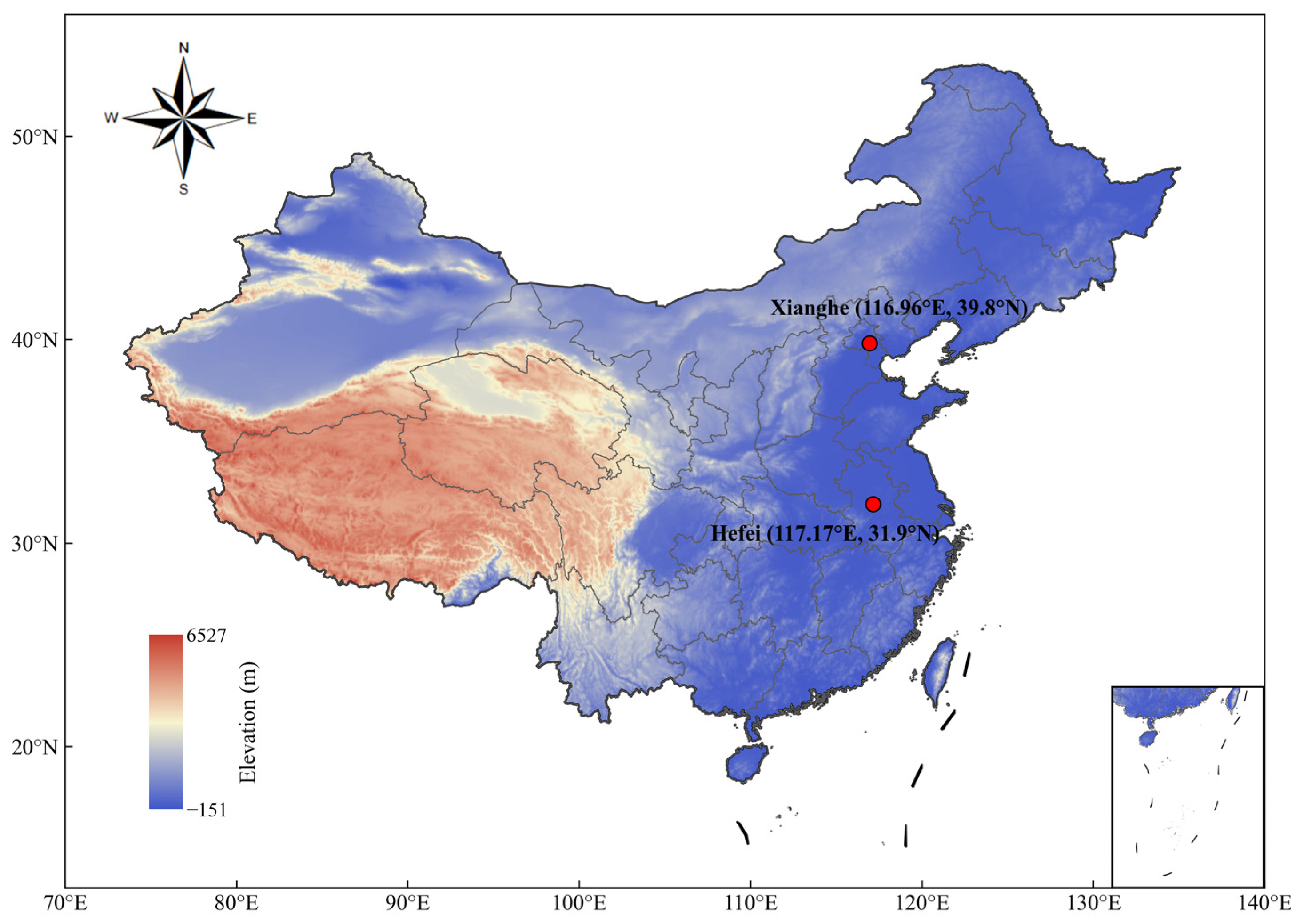
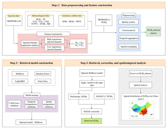
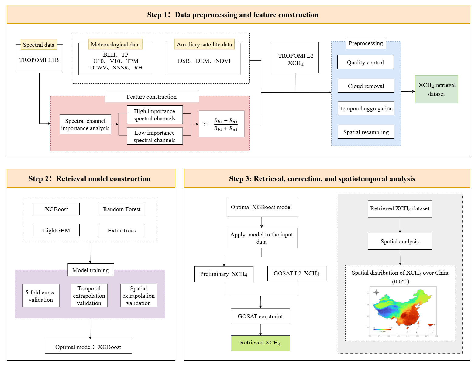
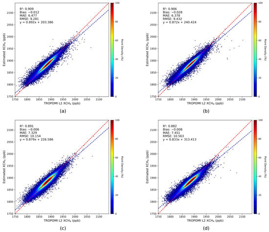
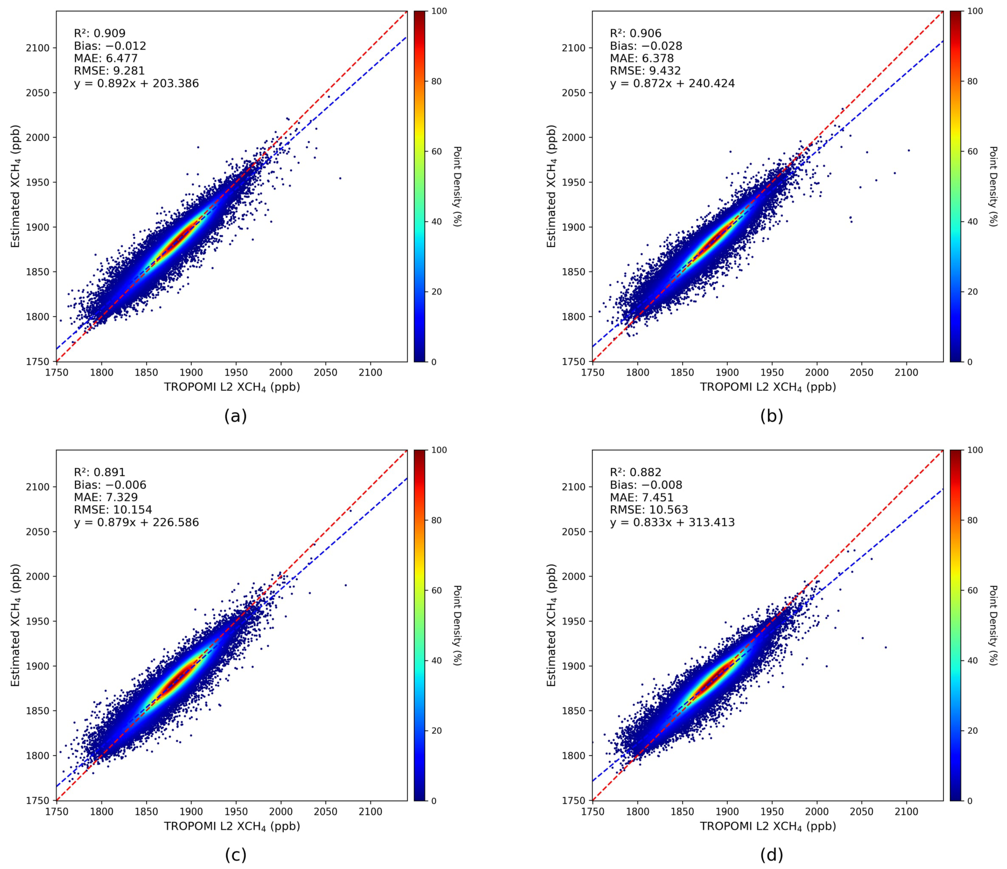
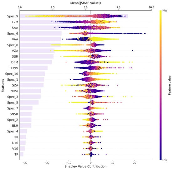
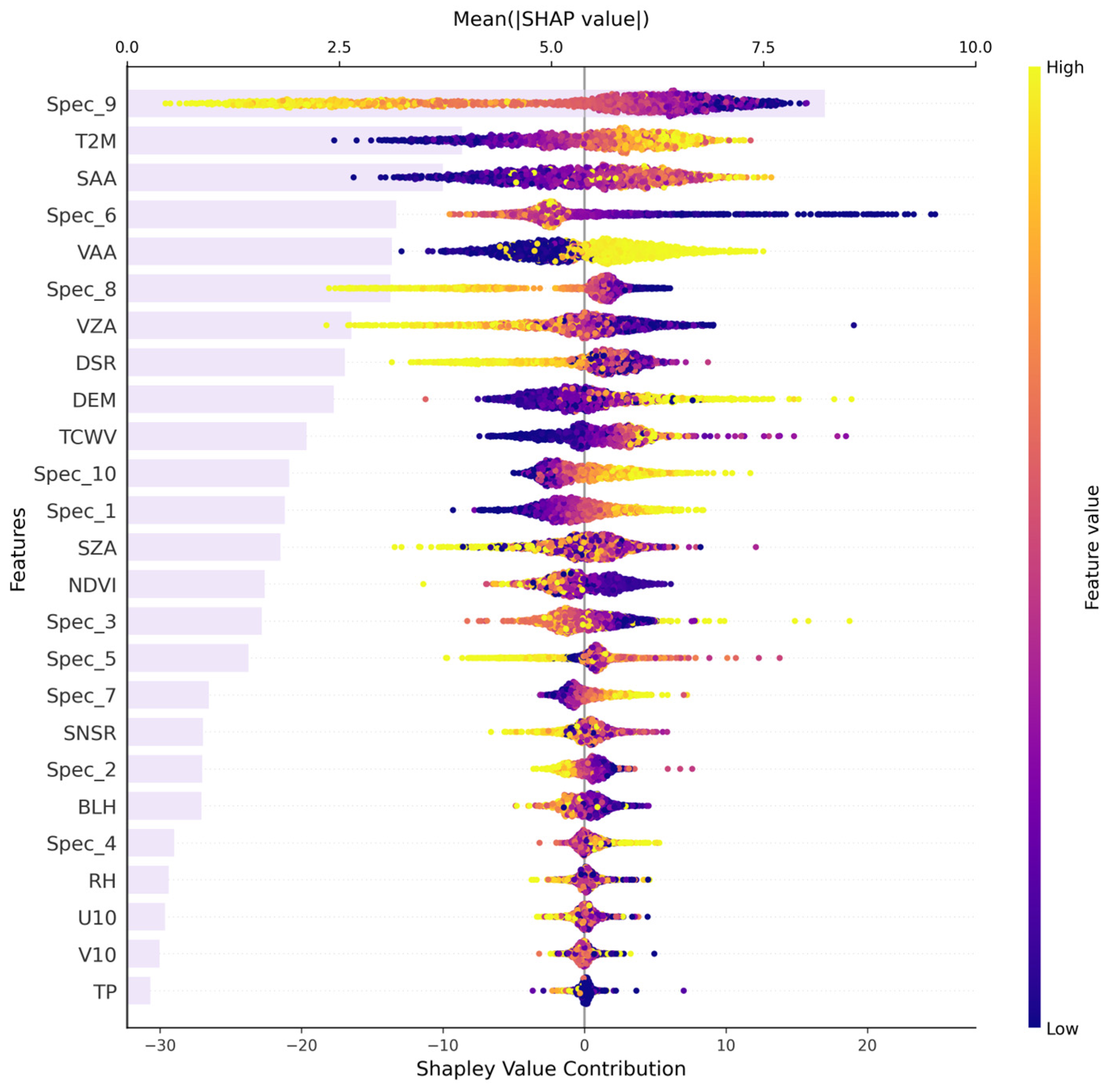
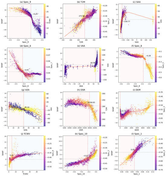
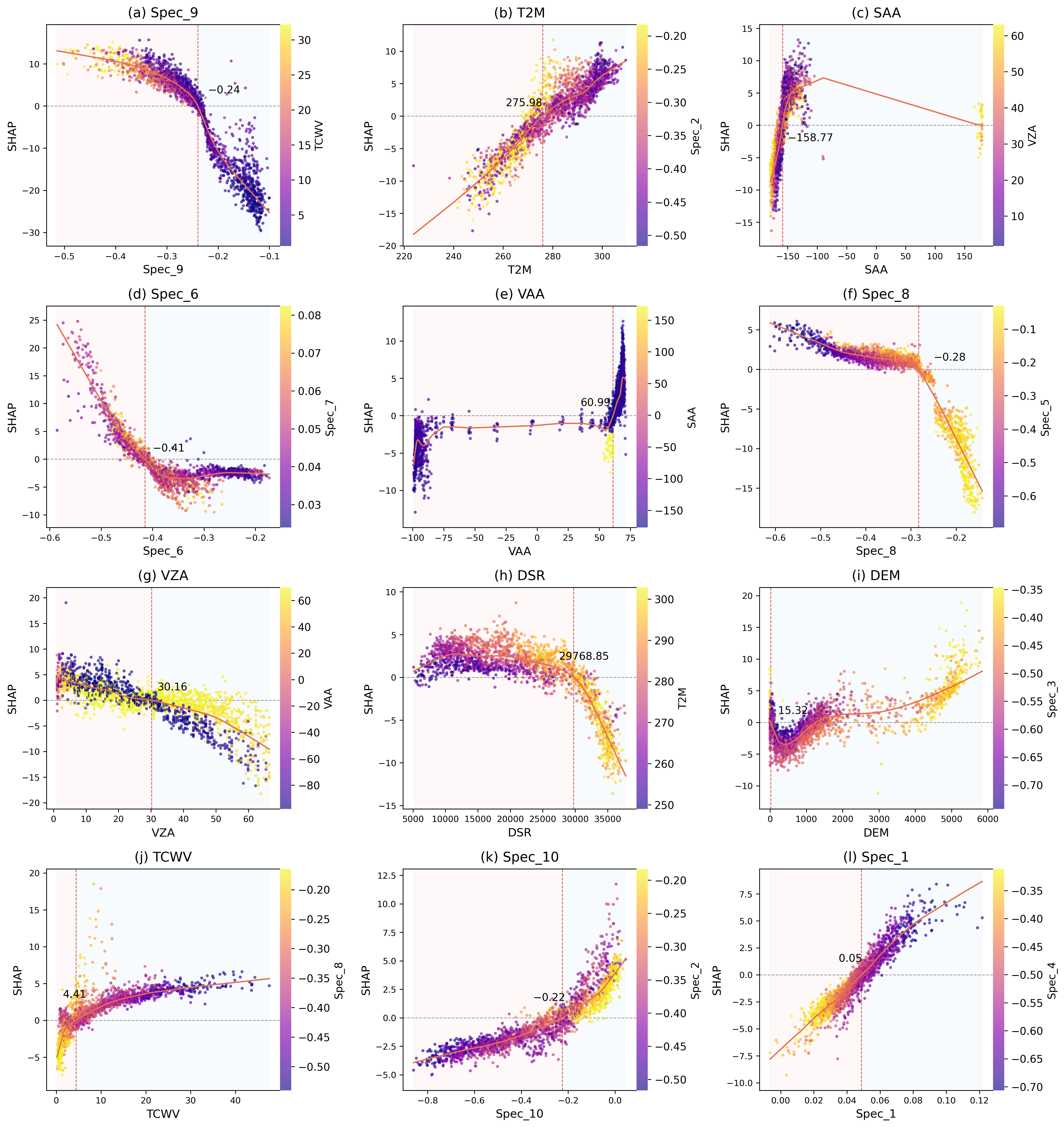
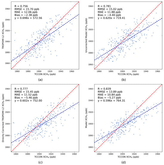
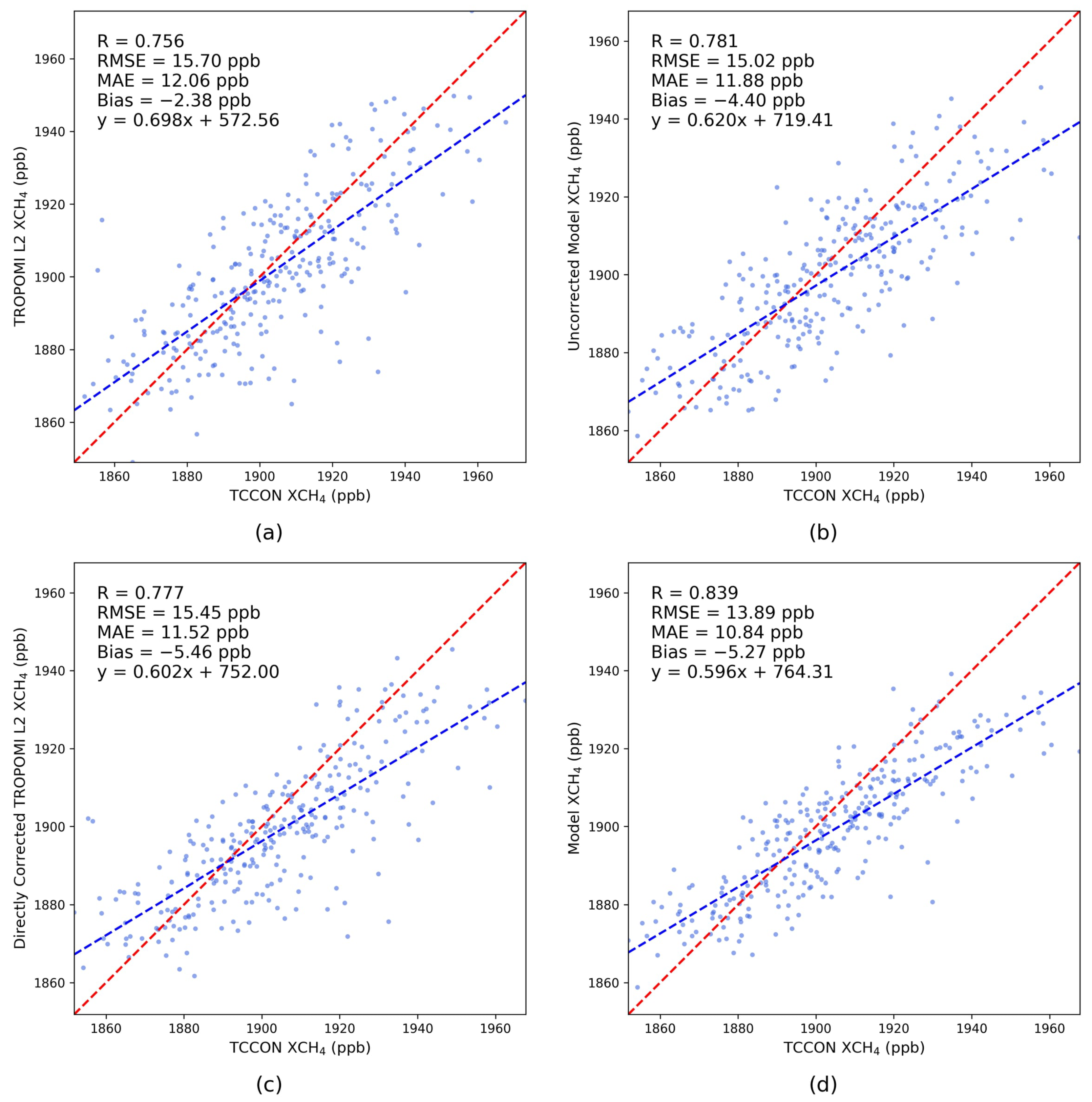
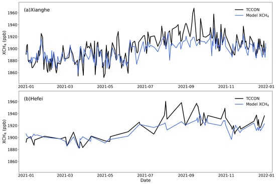
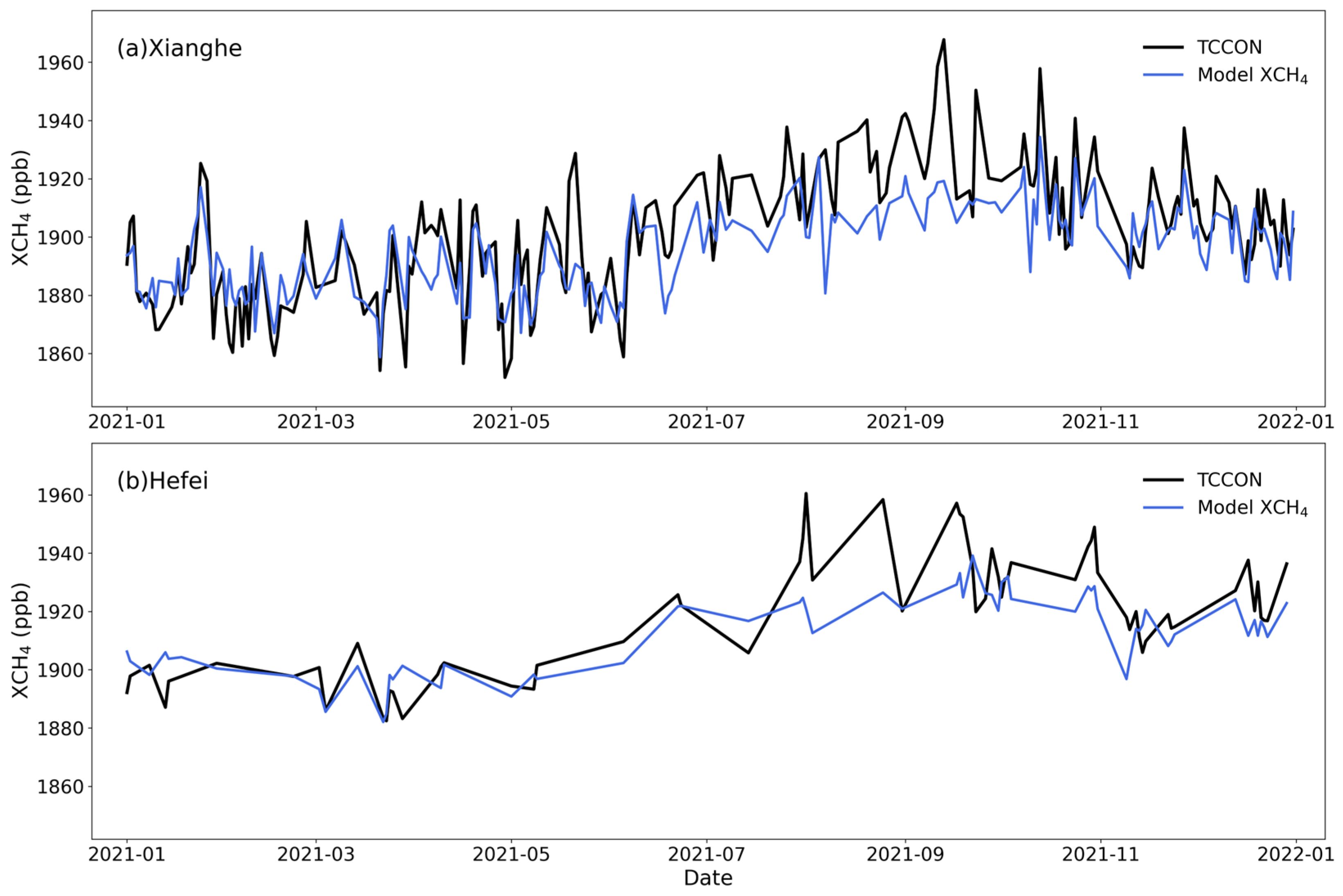
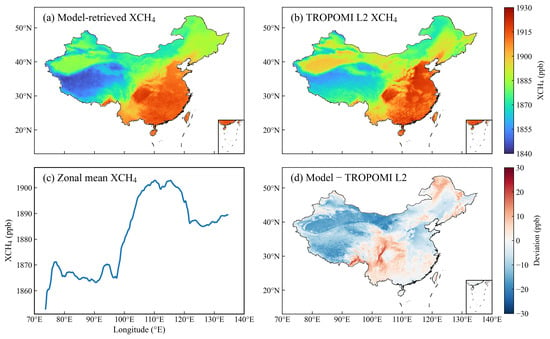
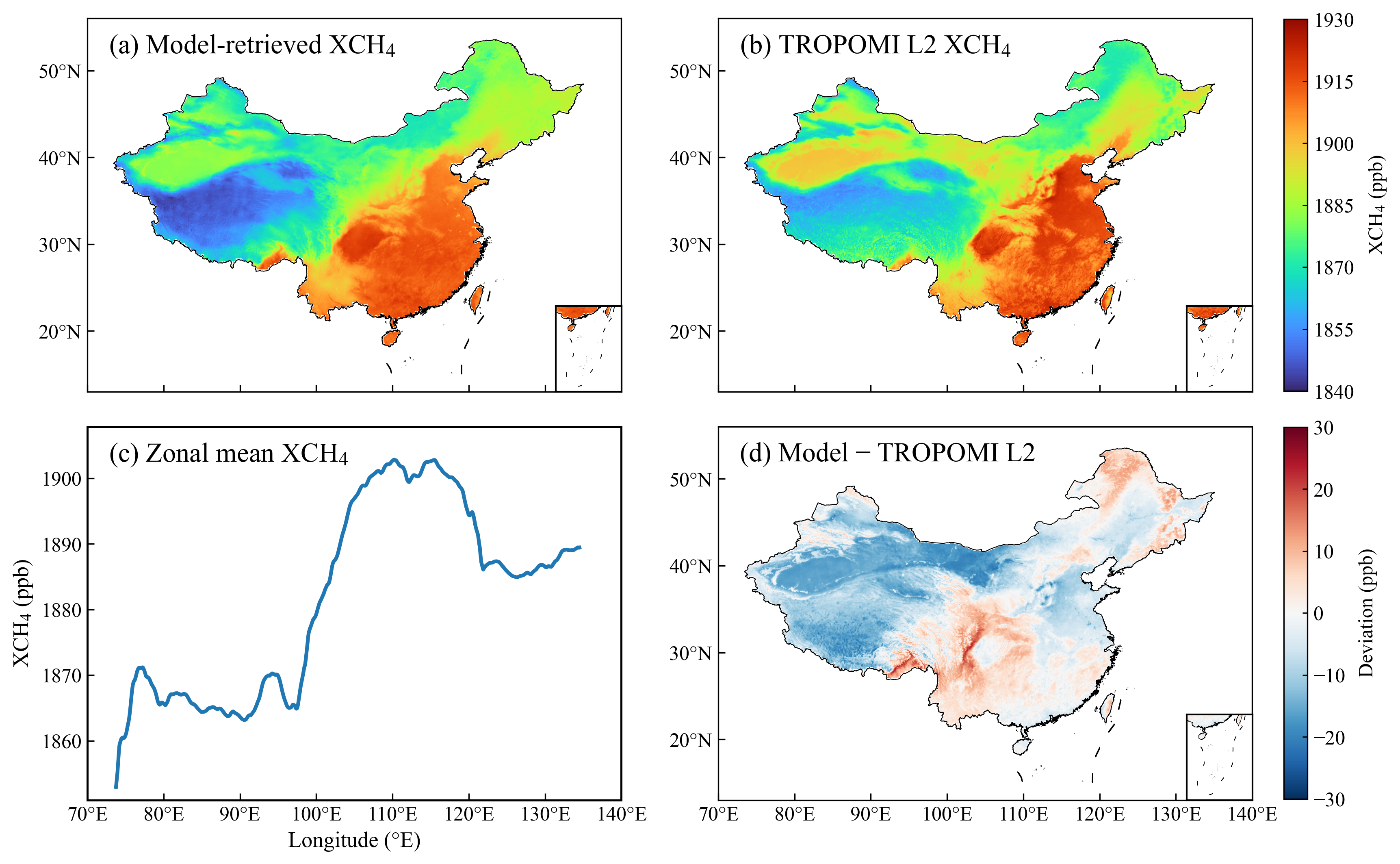
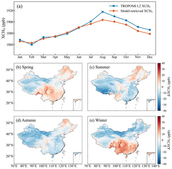
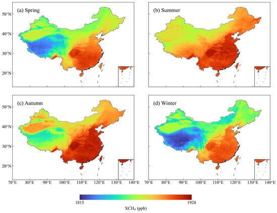
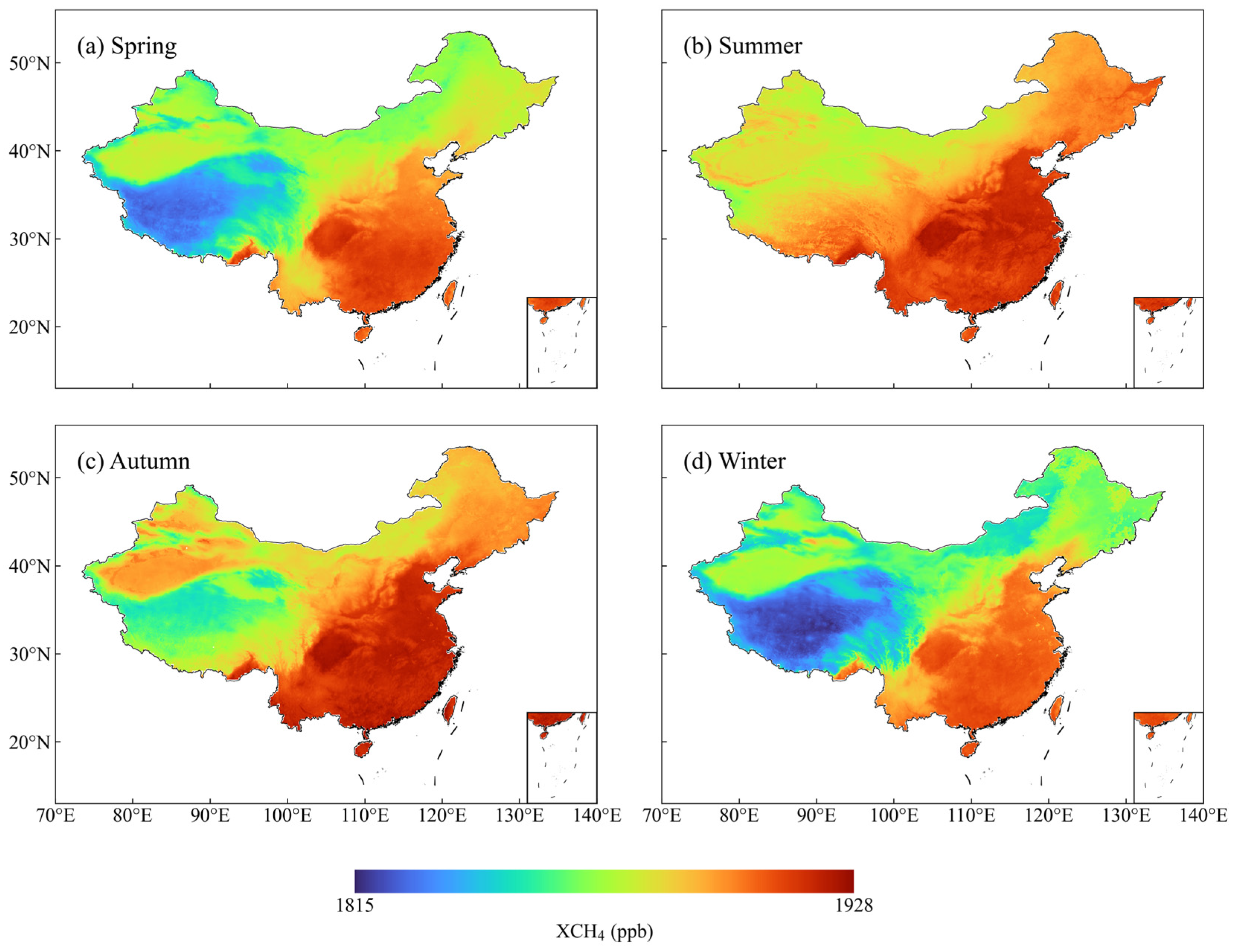
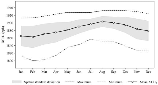
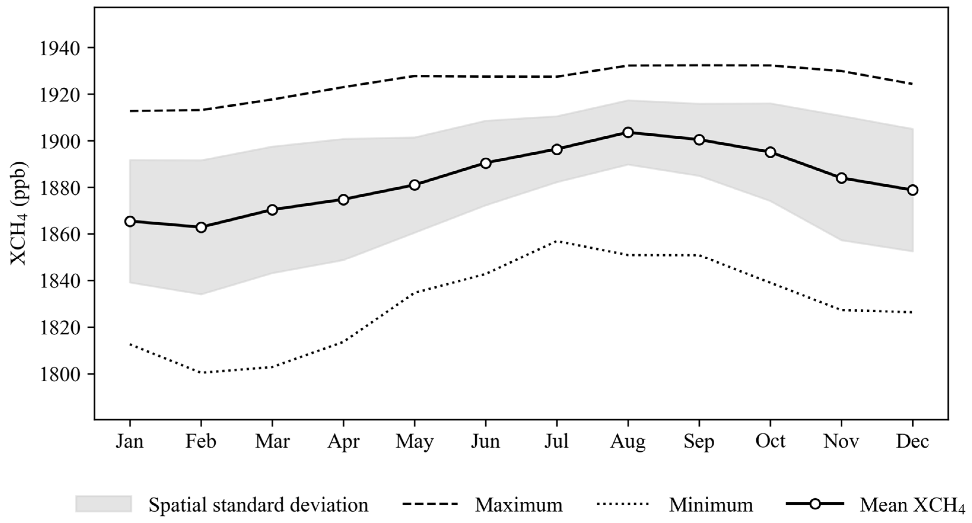
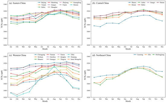
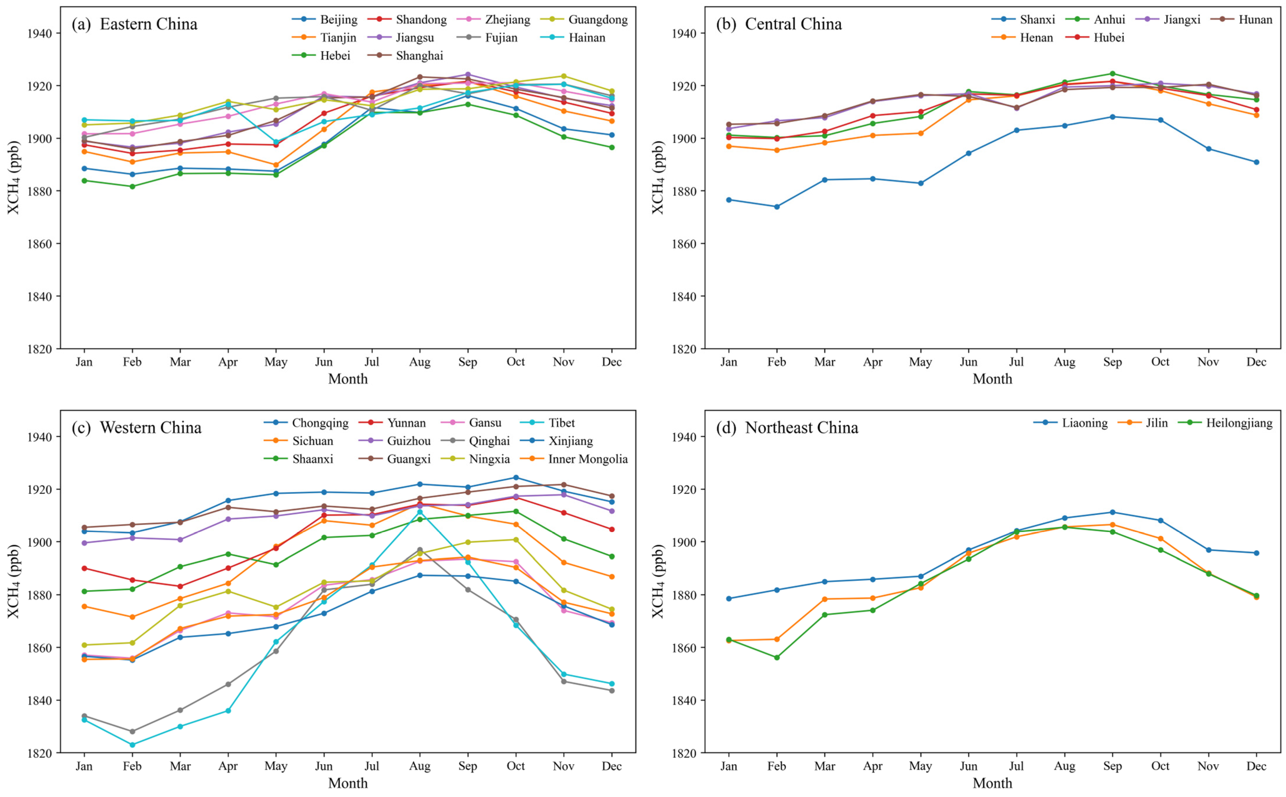

Disclaimer/Publisher’s Note: The statements, opinions and data contained in all publications are solely those of the individual author(s) and contributor(s) and not of MDPI and/or the editor(s). MDPI and/or the editor(s) disclaim responsibility for any injury to people or property resulting from any ideas, methods, instructions or products referred to in the content. |
© 2026 by the authors. Licensee MDPI, Basel, Switzerland. This article is an open access article distributed under the terms and conditions of the Creative Commons Attribution (CC BY) license.