


Abstract
Long-term monitoring of wetland degradation, recovery, and spatial resilience requires methods that can jointly exploit multi-temporal remote sensing observations and spatially heterogeneous environmental information. This study develops an intelligent remote sensing framework for monitoring the disturbance–recovery dynamics and spatial resilience of typical wetland landscapes in Northeast China by coupling Landsat-based Detection of Trends in Disturbance and Recovery (LandTrendr) with geographically weighted random forest (GWRF). Annual wetland landscape state sequences for 2000–2022 are constructed from multi-temporal Landsat observations and associated geospatial variables. LandTrendr time-series segmentation is used to identify disturbance timing, disturbance magnitude, recovery rate, and recovery duration, thereby converting long-term wetland change trajectories into quantitative indicators of degradation and recovery. At the GIS grid scale, remotely sensed vegetation and wetness indicators are integrated with wetland patch structure, hydrological conditions, topography, land-cover change, and anthropogenic pressure. GWRF then models local nonlinear relationships under spatial-distance weighting to generate a spatially explicit wetland resilience index and reveal geographically varying dominant controls. The LandTrendr–GWRF model achieved an R2 of 0.872, an RMSE of 0.057, and an MAE of 0.039, outperforming RF, GWR, XGBoost, and standalone GWRF benchmarks. The mean wetland resilience index was 0.641, with low-, medium-, and high-resilience areas accounting for 27.86%, 44.37%, and 27.77% of the study area, respectively. Significant spatial clustering was detected (Moran’s I = 0.421, Z = 6.92, p = 0.001). Hydrological regulation, landscape connectivity, fragmentation constraint, and anthropogenic disturbance pressure emerged as the four dominant spatial response types. High-resilience cells formed contiguous clusters where hydrological recharge and landscape connectivity were strong, while low-resilience cells clustered where fragmentation and construction pressure were concentrated. Disturbance magnitude and recovery duration differed markedly among the four response types, with connectivity-dominated cells returning to the pre-disturbance state within 4.4 years and anthropogenic pressure-dominated cells requiring 11.7 years. The proposed framework extends wetland remote sensing from static condition mapping toward process-oriented monitoring of degradation, recovery, connectivity, and resilience, providing a practical approach for long-term wetland restoration assessment and spatial management.
1. Introduction
Wetlands are dynamic ecosystems that support regional hydrological cycles, biodiversity, and ecological security, while providing key functions such as water conservation, flood regulation, carbon storage, and habitat maintenance [1,2,3]. Northeast China contains extensive marshes, river and lake wetlands, meadow wetlands, and coastal wetlands whose spatial patterns are closely related to black-soil protection, migratory-bird corridors, and the stability of cold-temperate ecological barriers. In recent decades, climate variability, land-use transformation, agricultural expansion, and engineering construction have altered wetland extent, patch structure, and hydrological connectivity, resulting in degradation, fragmentation, and reduced ecological connectivity in some regions [4,5,6]. These changes highlight the need for remote sensing approaches that can monitor not only where wetland change occurs, but also how wetland landscapes respond to disturbance and subsequently recover. Long-term spatial resilience monitoring is therefore important for identifying persistent degradation, evaluating restoration potential, and supporting regional wetland protection and adaptive management.
Monitoring wetland landscape resilience is challenging because it requires the integration of multi-source environmental information, long-term disturbance trajectories, and spatially heterogeneous response processes. Wetland conditions are jointly influenced by vegetation dynamics, surface moisture, hydrological recharge, topography, landscape connectivity, human activities, and climate variability. These factors operate at different spatial and temporal scales and often interact nonlinearly, making a single spectral index or a static landscape metric insufficient for characterizing resilience [7,8,9]. More importantly, resilience is a process property rather than a one-date condition: it depends on the magnitude of the disturbance, the speed and duration of recovery, and the environmental context in which recovery occurs [10,11,12]. Multi-temporal Earth observation offers the temporal continuity needed to trace these processes, whereas machine-learning and local spatial modeling provide tools for interpreting nonlinear and spatially nonstationary relationships. In Northeast China, the diversity and large spatial extent of wetlands make such an integrated monitoring strategy particularly necessary.
Wetland resilience monitoring is understood in this study as the repeated measurement of the capacity of a wetland landscape to absorb a disturbance and to return to a maintained state, and it is expressed through four quantities obtained from long-term observation, namely disturbance timing, disturbance magnitude, recovery rate, and recovery duration. Earlier assessments obtained this capacity from single-date spectral indices, from fixed-weight ecological zoning, or from landscape metrics computed on one land-cover map, and these approaches describe the condition of a wetland at one moment rather than the process by which it responds to disturbance [13,14,15,16,17,18,19,20,21,22]. Time-series algorithms improved the detection of change points and of trend segments, but they left the spatial controls of recovery unexplained [23,24,25]. The present study therefore defines the capacity at the grid scale as a composite of the four trajectory quantities and models it from multi-source environmental predictors with local machine learning, which connects the process measured in the time series to the spatial conditions under which recovery takes place.
Long-term wetland monitoring has developed along two separate lines. The first line extends single-date mapping into dense time series and relies on change detection to separate abrupt conversion from gradual degradation [23,24,25]. The second line builds multivariate indicators from several wetland parameters and analyzes their joint behavior with regression or machine learning [7,8,9]. The two lines have rarely been combined, so the trajectory of a wetland and the environmental conditions that govern that trajectory are usually reported in separate studies, and this separation is the gap addressed here.
Existing wetland remote sensing studies have addressed mapping, degradation assessment, ecological quality evaluation, landscape-pattern analysis, time-series change detection, and machine-learning modeling. Spectral indices such as NDVI, NDWI, and MNDWI are effective for monitoring vegetation and surface-water conditions, but applications based on individual dates or simple interannual comparisons generally describe state changes rather than post-disturbance–recovery trajectories [14,15,16]. GIS overlay, AHP, and entropy-weight methods support ecological zoning, yet their fixed weighting structures are limited in representing complex nonlinear responses [17,18,19]. Landscape metrics quantify fragmentation and connectivity but are often analyzed separately from long-term temporal disturbance information [20,21,22]. Time-series algorithms such as BFAST, CCDC, and LandTrendr can identify change points and trend segments, providing a stronger basis for monitoring wetland dynamics; however, when applied alone they provide limited explanation of spatially varying recovery controls [23,24,25]. Machine-learning methods such as RF and XGBoost can model nonlinear relationships, but conventional global models do not explicitly account for geographical nonstationarity. Accordingly, an important methodological need is to combine advanced time-series change detection with spatial machine learning and multi-source remote sensing/geospatial information so that wetland degradation, recovery, connectivity, and resilience can be monitored within one coherent framework.
This study has three objectives, which are to quantify long-term wetland disturbance and recovery in Northeast China from Landsat records spanning 2000 to 2022; to map the spatial resilience of wetland landscapes from multi-source environmental predictors with local machine learning; and to identify the environmental conditions that dominate resilience in different parts of the region. To meet these objectives, this study develops a long-term intelligent remote sensing framework that couples Landsat-based Detection of Trends in Disturbance and Recovery with geographically weighted random forest. First, multi-temporal Landsat observations are organized into annual wetland landscape state sequences, from which LandTrendr extracts disturbance occurrence time, disturbance magnitude, recovery rate, and recovery duration. Second, remotely sensed vegetation and wetness conditions are integrated at the GIS-grid scale with wetland patch structure, hydrological conditions, topography, land-cover transformation, and anthropogenic pressure to form a consistent multi-source predictor set. Third, GWRF introduces spatial-distance weighting into random-forest regression to model local nonlinear relationships, producing a spatially explicit resilience index and geographically varying variable-importance patterns. The framework therefore links time-series monitoring of wetland change with machine-learning-based spatial interpretation. Its main contribution is not simply to map a static resilience surface, but to represent wetland resilience through observable disturbance–recovery trajectories and to connect these trajectories with hydrological regulation, landscape connectivity, fragmentation, and human pressure. This process-oriented design is intended to support wetland degradation monitoring, restoration-priority identification, and spatially differentiated management in Northeast China.
2. Study Area, Data, and Methods
2.1. Study Area, Data Sources, and Sample Construction
This study focuses on typical wetland landscapes in Northeast China, which are defined here as the contiguous wetland concentration areas of Heilongjiang, Jilin, and Liaoning provinces that were retained by the delineation described below. The region spans cold-temperate to temperate monsoon environments and contains marshes, river and lake wetlands, meadow wetlands, and coastal wetlands. Strong spatial contrasts in hydrological recharge, vegetation condition, patch configuration, land-use pressure, and wetland connectivity make the region suitable for evaluating whether a long-term intelligent remote sensing framework can capture both temporal disturbance–recovery dynamics and geographically varying resilience patterns.
The region has a temperate continental monsoon climate with a mean annual temperature between minus four and ten degrees Celsius and mean annual precipitation between four hundred and one thousand millimeters, decreasing from southeast to northwest. Surface water is supplied by the Songhua, Nenjiang, Liaohe, and Yalu river systems together with numerous inland lakes and marsh complexes, and spring snowmelt and summer monsoon rainfall produce a marked seasonal water-level cycle. Wetland types in the region are marsh, river and lake wetland, meadow wetland, and coastal wetland, and their distribution is controlled by river flooding, groundwater depth, and the retreat of permafrost in the northern part of the region.
The monitoring extent was delineated from the 2022 CLCD wetland class. All wetland polygons larger than one hundred hectares within the three provinces were selected and merged, and the merged boundary was buffered by one kilometer to include the transition zone between wetland and upland. The resulting extent covers the marsh complexes of the Sanjiang Plain and the Xingkai Lake plain, the floodplains of the Songhua and Nenjiang rivers, the meadow wetlands of the Songnen Plain, the coastal wetlands of the Liaohe delta and the Yalu estuary, and the alpine marsh patches of the Changbai Mountains. The term typical wetland landscapes refers to these contiguous wetland concentration areas, which represent the four wetland types of the region and together cover the main wetland distribution of the three provinces. Grid cells were retained for modeling when wetland coverage reached fifty percent of the cell area. The location of the monitoring extent and the environmental setting of the three provinces are shown in Figure 1.
Figure 1.
Study area and environmental setting of the wetland monitoring extent in Northeast China. Panel a shows the position of Heilongjiang, Jilin, and Liaoning provinces within China, with the red dashed frame marking the monitoring extent. Panel b shows the elevation, the river network, the lakes and reservoirs, and the provincial boundaries of the monitoring extent, together with the wetland concentration areas referred to in the text.
The monitoring period covers 2000–2022. The data system combines Landsat Collection 2 Level-2 Surface Reflectance [26], the CLCD annual land-cover dataset of China [27], NASADEM Merged DEM Global 1 arc-second V001 [28], HydroSHEDS [29], OpenStreetMap on AWS [30], and basic GIS layers. Landsat provides the primary long-term Earth observation record for deriving NDVI, NDWI, and annual wetland landscape state sequences. CLCD provides annual land-cover information for wetland extent, patch structure, built-up land proportion, and land-use transition. NASADEM and HydroSHEDS provide topographic and hydrological context, while OpenStreetMap road data support characterization of anthropogenic pressure. The combination therefore integrates multi-temporal remote sensing with complementary geospatial information rather than treating all input sources as equivalent remote sensing products. The main datasets, derived variables, and model roles are summarized in Table 1.
Table 1.
Data and variable construction required for spatial resilience calculation in this paper.
Landsat observations were drawn from Landsat 5 Thematic Mapper, Landsat 7 Enhanced Thematic Mapper Plus, Landsat 8 Operational Land Imager, and Landsat 9 Operational Land Imager 2, all at Collection 2 Level-2 surface reflectance and 30 m resolution. Scenes acquired between June and September of each year were screened with the Collection 2 quality band and an object-based cloud and shadow mask, and the remaining clear observations were reduced to an annual median composite for each band. Landsat 7 scenes acquired after 2003 carry scan-line gaps, and these scenes were excluded from all years except 2012, when gap-filled Landsat 7 observations were used to bridge the interval between the end of Landsat 5 operations and the start of Landsat 8 operations. All sensors were cross-calibrated to the Landsat 8 reference through the Collection 2 surface reflectance coefficients before compositing. The CLCD annual land-cover dataset provides one map for each year from 2000 to 2022 at 30 m resolution, so it is temporally complete over the monitoring period and spatially consistent with the Landsat grid. HydroSHEDS was used at 15-arc-second resolution for river networks and basin boundaries, NASADEM at one-arc-second resolution for elevation and slope, and the OpenStreetMap road layer as a single snapshot for 2022. NASADEM elevation in flat marsh terrain was smoothed with a three-by-three median filter before the slope calculation to suppress stripe noise.
Data preprocessing was performed within a unified geospatial framework to ensure temporal and spatial comparability. Landsat imagery was processed into annual growing-season composites after radiometric and atmospheric correction, cloud-shadow removal, and image compositing. All datasets were transformed to a common projection and linked to the same grid system. DEM, land-cover, road, hydrological, and wetland patch data were resampled or summarized using appropriate spatial statistics, distance calculations, and overlay operations. This workflow preserves the 2000–2022 Landsat time series as the primary temporal monitoring signal while using ancillary datasets to provide environmental context for interpreting wetland change.
After preprocessing, regular GIS grids were used as the common sample units for time-series monitoring and spatial modeling. Wetland boundaries were overlaid with the grid system, and cells were retained when wetland coverage was at least 50%, the Landsat time series was sufficiently complete, and all required predictor variables were available. LandTrendr disturbance–recovery indicators and multi-source environmental variables were linked using identical grid units, producing a modeling dataset containing geographic location, remotely sensed wetland condition, environmental context, disturbance–recovery characteristics, and resilience target values. Model performance was assessed with two validation designs. The first design used a stratified random split of the modeling samples at a ratio of 7:3 between training and validation. Because wetland grids are spatially autocorrelated and neighboring cells share nearly identical predictors, a second design was added in which the study area was divided into blocks of 100 km by 100 km and fivefold cross-validation was performed with entire blocks assigned to a single fold, so that no validation cell shared a block with any training cell. All benchmark models were evaluated under both designs with identical folds, identical standardization rules, and identical evaluation metrics.
The grid size was set to 1000 m by 1000 m. This size keeps more than thirty Landsat pixels along each side of a cell, so annual composites and patch statistics remain stable within a cell, and it is close to the extent of a wetland patch group in the marsh complexes of the region, so a cell contains a landscape configuration rather than a single patch.
The aggregation rule was fixed for each predictor. Vegetation and wetness indices were computed for every 30 m pixel and then averaged within the cell. Elevation and slope were averaged. Distance to water and distance to roads were computed at 30 m and then averaged within the cell. Built-up proportion and land-use transition intensity were computed as area fractions from the annual land-cover maps. Patch density and the connectivity index were computed from the wetland patches clipped to each cell.
2.2. Overall Framework Design
This study constructed an intelligent remote sensing framework for monitoring wetland landscape resilience by integrating multi-temporal Earth observation, multi-source geospatial covariates, time-series segmentation, and local machine learning. GIS grid cells were used as common analysis units to register multi-temporal Landsat imagery, annual land-cover information, hydrological data, topographic data, landscape-pattern metrics, and anthropogenic disturbance indicators. LandTrendr was used to identify long-term disturbance–recovery trajectories from annual wetland state sequences, while GWRF characterized spatially nonstationary and nonlinear relationships between resilience and its environmental controls. The outputs included grid-scale wetland resilience, resilience-level zoning, and local variable-importance patterns. In this way, the framework moves from remote sensing observation of wetland condition to process-oriented monitoring of disturbance, recovery, and spatial resilience. The overall workflow is shown in Figure 2.
Figure 2.
Intelligent remote sensing and GIS framework for long-term monitoring and spatial modeling of wetland landscape resilience. Every symbol used in the framework is defined in Section 2.2, Section 2.3, Section 2.4 and Section 2.5, and the wetland landscape spatial resilience index is the predicted value of the GWRF model described in Section 2.5.The arrows indicate the direction of data processing and information flow between the components of the framework.
Intelligent remote sensing is used here in a restricted sense. It denotes the joint use of algorithmic time-series segmentation that extracts process indicators without manual interpretation and a local machine-learning regression that adapts its parameters to each location. The artificial intelligence component of the framework is the geographically weighted random forest, which supplies the nonlinear fitting and the spatial weighting, and the segmentation step supplies the training target. No deep learning model is used, and the term is not intended to describe a general platform for automated image interpretation.
In the framework, a multi-source environmental feature vector connects remote sensing observations and ancillary geospatial information with resilience modeling. The study area is divided into GIS grid units, and the environmental characteristics of grid cell s in year t are represented by vegetation cover, wetland water status, landscape structure, topographic conditions, hydrological conditions, and anthropogenic disturbance, as shown in Equation (1):
In Equation (1), Xs,t denotes the multi-source environmental feature vector of grid cell s in year t; NDVIs,t represents vegetation cover derived from Landsat; NDWIs,t represents wetland water status derived from Landsat; Fs,t represents landscape fragmentation; PCs,t represents ecological connectivity; DEMs represents elevation; Slopes represents slope; Hs,t represents hydrological conditions; Us,t represents anthropogenic disturbance intensity; and T denotes vector transposition. The vector integrates remotely sensed wetland condition with landscape and environmental context, providing a consistent predictor basis for subsequent time-series disturbance detection and spatial resilience modeling.
Within this framework, wetland landscape resilience is interpreted as a spatially explicit outcome of long-term disturbance–recovery dynamics and current environmental conditions. LandTrendr contributes temporally explicit indicators, including disturbance occurrence time, disturbance magnitude, recovery rate, and recovery duration. GWRF then models local nonlinear relationships using spatial-distance weights, while GIS grids provide a common support for multi-source data integration and spatial output. The resulting workflow establishes a continuous link from Earth observation and time-series monitoring to resilience estimation and interpretation of geographically varying controls.
Resilience is therefore treated as an attribute of a process rather than a condition observed on a single date. A wetland grid that returns to its pre-disturbance state within a short interval is more resilient than a grid that remains below that state for a long interval, even when the two grids carry the same current spectral condition. The three trajectory quantities of disturbance magnitude, recovery rate, and recovery duration carry this process information, and the environmental predictors describe the conditions under which recovery takes place, so the composite of the three quantities is used as the observed resilience of a grid and the environmental predictors are used to model where that resilience is high or low.
2.3. Multi-Source Remote Sensing and Environmental Covariate Extraction
Multi-source variable extraction was used to convert remote sensing imagery and ancillary hydrological, topographic, landscape-structural, and anthropogenic information into a unified set of predictors. GIS grid cells were used as the common spatial support. Multi-temporal Landsat imagery was processed through radiometric correction, atmospheric correction, cloud and shadow removal, annual compositing, and spatial registration to maintain temporal consistency. Landsat-derived indices characterized vegetation cover and surface wetness; annual wetland patch information was used to calculate fragmentation and ecological connectivity; DEM data represented elevation and slope; hydrological data characterized water proximity and recharge conditions; and land-cover and road information represented external development pressure. This integration preserved the direct remote sensing signal while adding the spatial context needed to interpret wetland disturbance and recovery.
Vegetation cover reflects the growth status of wetland vegetation. This study used the normalized difference vegetation index for characterization, and its calculation form is shown in Equation (2):
In Equation (2), the normalized difference vegetation index of grid cell s in year t is denoted by NDVIs,t; the near-infrared reflectance is denoted by ρNIRs,t; and the red-band reflectance is denoted by ρReds,t. A higher NDVIs,t value indicates better wetland vegetation cover and growth status.
The wetland water state reflects the hydrological maintenance conditions of the wetland landscape. This study used the normalized difference water index for characterization, and its calculation form is shown in Equation (3):
In Equation (3), the normalized difference water index of grid cell s in year t is denoted by NDWIs,t, the green band reflectance is denoted by ρGreens,t, and the near-infrared reflectance is denoted by ρNIRs,t. The numerical variation of NDWIs,t was used to characterize the wetland moisture state and surface moisture level.
Landscape fragmentation was used to characterize the degree to which wetland patches are fragmented. In this study, patch density was used to characterize it, and its calculation form is shown in Equation (4):
In Equation (4), the landscape fragmentation of grid cell s in year t is denoted by Fs,t, the number of wetland patches within the cell is denoted by Ns,t, and the area of the cell is denoted by As. A larger Fs,t value indicates more wetland patches per unit area and a stronger segmentation of the landscape.
Ecological connectivity reflects the strength of spatial connections between wetland patches. This study used the probabilistic connectivity index for characterization, and its calculation form is shown in Equation (5):
in Equation (5), the ecological connectivity index of grid cell s in year t is denoted by PCs,t, the areas of wetland patches i and j are denoted by ai and aj, the connection probability between the two patches is denoted by pij, the total landscape area is denoted by A, and the total number of wetland patches is denoted by n. A larger PCs,t value indicates a closer spatial connection between wetland patches and greater integrity of the landscape structure.
Hydrological conditions Hs,t and anthropogenic disturbance intensity Us,t were uniformly expressed at the GIS grid scale. Hs,t was comprehensively characterized by the humidity state within the grid, proximity to water bodies, and intensity of hydrological recharge, reflecting the water maintenance conditions of the wetland landscape. Us,t was comprehensively expressed by the proportion of built-up land, road distance, and intensity of land-use transformation, reflecting the pressure of external development activities on the stability and the restoration process of the wetland landscape. Hs,t, Us,t, NDVIs,t, NDWIs,t, Fs,t, and PCs,t together constitute the environmental perception factor system for resilience modeling.
Because the multi-source environmental variables differ in units and numerical ranges, all factors were standardized to a common interval before model integration. The standardization is shown in Equation (6):
In Equation (6), Zs,k represents the standardized value of the kth environmental variable in grid cell s; Xs,k is the original value; Xk,max and Xk,min are the maximum and minimum values of the kth factor, respectively; and ck represents the directional attribute, with ck = +1 for a positive factor and ck = −1 for a negative factor. Standardization places remotely sensed and ancillary geospatial predictors on a comparable scale for LandTrendr–GWRF modeling.
After preprocessing the remote sensing, land-cover, hydrological, topographic, and anthropogenic data, all variables were registered to the same GIS grid system and summarized by spatial overlay, attribute assignment, and standardization. This step produces a consistent multi-source feature matrix containing vegetation, wetness, fragmentation, connectivity, hydrological conditions, and anthropogenic pressure. The gridded representation enables long-term remote sensing trajectories and spatial environmental covariates to be linked at the same analysis unit, providing the data foundation for disturbance–recovery monitoring and local machine-learning modeling. The integrated feature representation is shown in Figure 3.
Figure 3.
GIS gridded integration of multi-source remote sensing and environmental variables. Panel (a) shows the complete modeling grid over the wetland monitoring extent of Northeast China, with every retained cell displayed at the analysis resolution. Panel (b) shows the standardized environmental factor matrix of the retained cells.
As shown in Figure 3, wetland grid cells exhibit clear spatial differences in the integrated predictor set. Cells with favorable hydrological conditions, stronger ecological connectivity, and lower human disturbance generally show stronger ecological support, whereas cells with greater fragmentation, construction influence, or weak water-retention capacity show less favorable conditions. Figure 3a illustrates how a common GIS grid integrates information from remote sensing and ancillary datasets, while Figure 3b shows standardized differences among variables across representative cells. This gridded integration is important for intelligent wetland monitoring because it links spectral and land-cover observations with the spatial context required to explain why disturbance and recovery trajectories vary among locations.
2.4. LandTrendr-Based Wetland Disturbance–Recovery Time-Series Monitoring
LandTrendr time-series analysis was used to monitor long-term wetland landscape change and to convert annual remote sensing trajectories into disturbance–recovery indicators. GIS grid cells were treated as time-series units. After annual compositing, outlier removal, and spatial registration, a wetland landscape state index Ys,t was constructed for grid cell s in year t by integrating standardized vegetation cover, wetland water status, ecological connectivity, landscape fragmentation, hydrological conditions, and anthropogenic disturbance after directional consistency processing. The resulting annual sequence represents the evolving wetland landscape condition: decreases indicate degradation or intensified disturbance, whereas sustained increases after a low point indicate recovery. This formulation enables the monitoring focus to shift from isolated wetland states toward the timing and trajectory of change.
Here, the wetland landscape state index is a composite of the six standardized predictors described in Section 2.3 rather than a single spectral index. Vegetation cover, wetland water status, ecological connectivity, and hydrological condition entered the composite with a positive sign, while landscape fragmentation and anthropogenic disturbance entered with a negative sign. The index of a grid cell in a given year is the arithmetic mean of these six directionally consistent standardized values, as written in Equation (7), so the index is bounded between zero and one, and larger values denote a better maintained wetland landscape state. This definition retains the sensitivity of Landsat reflectance to vegetation and surface water while adding patch structure, hydrological support, and human pressure, and it keeps the state sequence on the same directional scale as the spatial predictors used later in the model.
LandTrendr fitted wetland landscape state index sequences with a finite number of linear segments, which reduced the impact of short-term noise while preserving long-term trends [31,32,33]. Assuming the state sequence of grid cell s satisfies a linear relationship in the m-th time segment, its piecewise fitting form is shown in Equation (8):
Ys,t = αs,m + βs,mt + εs,t t ∈ [τm−1,τm]
In Equation (8), Ys,t represents the wetland landscape state index of grid cell s in year t; αs,m represents the intercept term of the m-th segment; βs,m represents the slope of the m-th segment; εs,t represents the fitting residual; τm−1 and τm represent the starting and ending nodes of the m-th segment, respectively. The sign and magnitude of βs,m were used to determine the direction and intensity of wetland landscape state changes; a negative slope corresponds to a state decline process, and a positive slope corresponds to a state recovery process.
In the piecewise fitting results, when the slope of the decreasing state index segment is negative and the decrease between nodes reaches the perturbation identification threshold, the segment is identified as a perturbation segment; when the slope of the segment after perturbation is positive and the state index continues to rise, the segment is identified as a recovery segment. The perturbation amplitude is represented by the state difference between the stable node before perturbation and the low-value node after perturbation, and its calculation form is shown in Equation (9):
In Equation (9), Ds represents the disturbance amplitude of grid cell s; Ys,τb represents the wetland landscape state index corresponding to the stable node τb before the disturbance occurs; Ys,τd represents the wetland landscape state index corresponding to the low-value node τd after the disturbance; max(·) represents the maximum value function.
The recovery rate is represented by the increase in the wetland landscape state index per unit time during the recovery phase. It is used to characterize the intensity of the wetland landscape state recovery after disturbance, and its calculation form is shown in Equation (10):
In Equation (10), Vs represents the recovery rate of grid cell s; Ys,τr represents the wetland landscape state index corresponding to node τr at the end of the recovery period; Ys,τd represents the wetland landscape state index corresponding to node τd after the disturbance; and τr − τd represents the recovery duration. The higher the value of Vs, the faster the wetland landscape recovers after the disturbance.
After the multi-source variables were organized at the GIS-grid scale, the annual wetland landscape state index was used to construct a 2000–2022 monitoring sequence for each valid grid cell. LandTrendr performs piecewise segmentation to distinguish stable, declining, and recovering phases and to extract disturbance occurrence time, disturbance magnitude, recovery rate, and recovery duration. By suppressing short-term interannual noise while retaining persistent trajectory changes, this procedure provides process-oriented remote sensing indicators that can distinguish transient fluctuations from sustained degradation and recovery. These time-series indicators are subsequently combined with spatial environmental covariates in GWRF. Representative disturbance–recovery monitoring results are shown in Figure 4.
Figure 4.
Piecewise fitting of wetland landscape disturbance–recovery time series. (a) LandTrendr segmented fitting of a typical wetland grid. (b) Extracted disturbance–recovery variables of selected grids.
As shown in Figure 4, the annual state sequence of a representative wetland grid is characterized by alternating stable, declining, recovering, and post-recovery phases rather than monotonic change. The observed interannual fluctuations reflect variability in vegetation condition, surface wetness, hydrological recharge, and external disturbance, whereas LandTrendr summarizes the dominant long-term trajectory as interpretable segments. A sustained decline identifies a degradation phase, while a positive post-disturbance segment identifies recovery. Figure 4b further demonstrates marked spatial differences in disturbance magnitude and recovery duration among wetland grids. Cells with smaller disturbance magnitude and shorter recovery duration are generally associated with stronger hydrological support or connectivity, whereas cells with larger disturbances and prolonged recovery are more frequently associated with fragmentation, human pressure, or unstable hydrological conditions. Thus, LandTrendr provides more than change-point detection: it converts long-term wetland remote sensing observations into quantitative indicators of degradation and restoration dynamics that can be mapped and interpreted spatially.
2.5. GWRF Machine-Learning Modeling of Spatial Wetland Resilience
GWRF was used as the machine-learning component of the framework to model nonlinear and spatially nonstationary relationships between wetland resilience and the integrated predictor set. Each GIS grid cell was treated as a modeling unit. Standardized environmental variables from Section 2.3 and disturbance–recovery indicators from Section 2.4 jointly form the input set, while wetland landscape resilience is the model target. Unlike a conventional global random forest, GWRF introduces geographical weighting and constructs a local training neighborhood for each target cell so that nearby samples exert greater influence than distant samples. This structure is appropriate for large-area wetland monitoring because hydrological conditions, landscape configuration, and anthropogenic pressure can have different relationships with resilience across geographic space [34,35,36].
The geographical weighting used here follows the spatially local ensemble formulation developed for gradient boosted trees in regional regression, in which a kernel weighted neighborhood replaces the global training set [13].
Let so be the target grid cell whose spatial resilience is to be estimated, si be the sample cell participating in local training, d(si, so) represent the spatial distance between the sample cell and the target cell, and b represent the spatial bandwidth. GWRF constructed a weighted local training sample set corresponding to the target grid through a spatial weight function and trained a random forest regression model on this sample set. Its calculation form is shown in Equation (11):
In Equation (11), wi(so) represents the spatial weight of the training sample si relative to the target grid so; d(si,so) represents the spatial distance between them; b is the bandwidth parameter; so represents the predicted wetland landscape spatial resilience of the target grid so; B represents the number of regression trees in the random forest; Tq represents the q-th regression tree; Zso represents the standardized input variable vector of the target grid s o; and Sw (so) represents the local training sample set formed by the spatial weight wi (so). In this formula, the spatial weight was used to control the intensity of the sample’s participation in the local model, and the random forest ensemble term was used to output the resilience estimation result of the target grid.
At the model-input level, Landsat-derived vegetation and wetness indicators, landscape fragmentation, ecological connectivity, topography, hydrological conditions, and anthropogenic disturbance formed the spatial environmental predictors, while disturbance occurrence time, disturbance magnitude, recovery rate, and recovery duration formed the temporal-process predictors. GWRF learned local nonlinear mappings between these inputs and wetland resilience under spatial weighting. Consequently, the model combines the temporal sensitivity of LandTrendr with the nonlinear learning capacity of random forests and the spatial adaptability of geographically weighted modeling, enabling the remote sensing framework to characterize both long-term wetland dynamics and local spatial heterogeneity.
Following LandTrendr disturbance–recovery extraction, GWRF was used to translate the combined time-series and environmental information into spatially explicit resilience estimates. The geographical weighting step ensures that local wetland neighborhoods contribute more strongly to each prediction, reducing the tendency of global models to smooth over regional differences. To support interpretation rather than treating machine learning as a black box, the GWRF outputs are examined through local spatial weights, ecological support-disturbance pressure relationships, and response-specific variable importance, as shown in Figure 5. This design links intelligent prediction with ecological interpretation, which is important for converting remote sensing monitoring results into restoration and management information.
Figure 5.
Spatial response of local variable importance in GWRF. (a) Local spatial weighting kernel of GWRF. (b) Ecological support-disturbance pressure response space. (c) Response-specific importance profiles.
As shown in Figure 5, GWRF reveals pronounced local differences in the environmental controls associated with wetland resilience. The spatial kernel in Figure 5a gives greater weight to neighboring wetland cells, allowing the model to retain geographic heterogeneity. Figure 5b positions cells along gradients of ecological support and disturbance pressure, while Figure 5c shows that hydrological regulation, landscape connectivity, fragmentation, and anthropogenic disturbance contribute differently across locations. These patterns demonstrate the value of spatial machine learning for wetland monitoring: the model not only estimates where resilience is high or low, but also indicates which local environmental constraints are most strongly associated with observed disturbance–recovery behavior.
2.6. Spatial Resilience Mapping and Dominant Spatial Response Identification
The spatial resilience index was generated from the GWRF output for each wetland grid cell. Standardized environmental predictors and LandTrendr-derived disturbance–recovery indicators were entered into the model, and the predicted value from Equation (11) was used as the spatial resilience index. Because the predictor set contains both current wetland condition and long-term disturbance–recovery information, the resulting map represents a process-informed monitoring product rather than a single-date ecological status map. It summarizes the combined effects of environmental conditions, historical disturbance intensity, and recovery response capacity [37,38].
The reference resilience value used as the modeling target is a composite of the three trajectory quantities obtained from the LandTrendr segmentation. Disturbance magnitude enters the composite with a negative sign, recovery rate enters with a positive sign, and recovery duration enters with a negative sign. The composite is then rescaled to the interval from zero to one so that larger values denote a stronger capacity to return to the pre-disturbance state. The GWRF prediction for a grid cell is reported as the wetland landscape spatial resilience index, and this is the quantity labeled in Figure 2 and mapped in Section 3.4.
In classifying resilience levels, this study used a grid-scale spatial resilience index and the natural discontinuity method to divide the study area into low-resilience, medium-resilience, and high-resilience zones. The classification results are used to express the spatial differentiation pattern of resilience in typical wetland landscapes in Northeast China and provide a basis for subsequent ecological risk identification, restoration priority zone determination, and spatial management.
The identification of spatial response types is based on a combination of resilience level, LandTrendr disturbance–recovery characteristics, and the importance of local variables in GWRF. Resilience level reflects the overall recovery status of the wetland landscape; disturbance amplitude, recovery rate, and recovery duration reflect the dynamic response process of the wetland landscape; and the importance of local variables reflects the dominant factors in resilience formation within different grid cells. Based on the spatial overlay of the above information and using the category of factors with dominant local variable importance as the criterion, this study grouped wetland grid cells into four spatial response types, namely, hydrological regulation, landscape connectivity, fragmentation constraint, and anthropogenic disturbance pressure. These types describe statistical associations between local predictor importance and disturbance–recovery behavior, and they are not presented as verified causal mechanisms.
This procedure integrated process monitoring, resilience mapping, hierarchical zoning, and dominant-factor interpretation within one spatial analysis framework. The resulting products provide a direct pathway from long-term remote sensing observations to maps of degradation-recovery condition and spatial resilience, supporting the identification of vulnerable wetland areas, restoration priorities, and differentiated management strategies.
2.7. Model Parameters and Experimental Scheme
To ensure a unified experimental basis for LandTrendr disturbance–recovery identification and GWRF spatial resilience modeling, this study completed the model parameter configuration and experimental design at the GIS grid scale. LandTrendr used the annual wetland landscape state index from 2000 to 2022 as the input sequence, with a maximum number of segments set to 6, a disturbance identification threshold set to 0.10, a recovery identification threshold set to 0.08, a short-term peak suppression parameter set to 0.90, a maximum node redundancy set to 3, a fitting significance threshold set to 0.05, and a model optimization ratio set to 0.75 to ensure the stability of the time-series segmentation results. The complete parameter set is listed in Table 2.
Table 2.
Parameter settings of the LandTrendr segmentation and the geographically weighted random forest.
The main parameters of GWRF include local spatial bandwidth and random forest structure. The number of random forest regression trees was set to 500, the minimum number of samples per node was set to 5, and the maximum number of features was determined by the square root of the number of input variables. The spatial bandwidth adopted an adaptive neighborhood approach, selecting the 120 nearest valid samples from each target grid to construct a local training set and using a Gaussian kernel function to calculate spatial-distance weights, so that neighboring samples had a higher influence in the local model.
Model training employed a unified sample partitioning and standardization rule. Training and validation samples were spatially stratified and sampled at a 7:3 ratio, with a fixed random seed to ensure reproducibility of experimental results. To verify the effectiveness of the LandTrendr–GWRF model, RF, GWR, XGBoost, and GWRF were used as benchmark models and were compared under the same training and validation sets, input variable standardization rules, and evaluation metric system. To further analyze the contributions of the model components, ablation experiments were conducted to remove LandTrendr, geographical weighting, landscape structure variables, and anthropogenic interference variables.
Furthermore, this study conducted parameter sensitivity analysis on the LandTrendr maximum number of segments, perturbation identification threshold, and GWRF spatial bandwidth to verify the model’s stability in response to changes in key parameters. The natural breakpoint method was used to classify resilience levels, and Moran’s I and LISA local spatial autocorrelation methods were combined to examine the spatial clustering characteristics of the resilience index, providing a basis for subsequent spatial differentiation and spatial response analysis.
2.8. Accuracy Evaluation and Spatial Statistical Indicators
To evaluate the predictive performance of the wetland landscape spatial resilience model, this study used the coefficient of determination, root mean square error (RMSE), and mean absolute error (MAE) as accuracy evaluation indicators. The coefficient of determination measures the model’s ability to explain spatial differences in resilience target values; a higher value indicates a better model fit. The root mean square error reflects the overall dispersion of prediction errors, and a lower value indicates a smaller magnitude of large errors. The MAE measures the average deviation between predicted and reference values; a lower value indicates smaller overall model error.
These three indicators are appropriate because the resilience target is a continuous variable bounded between zero and one, so a prediction error is a difference on a defined and interpretable scale rather than a class label that is either right or wrong. The coefficient of determination reports the share of spatial variance in the target that the model reproduces. The root mean square error reports the magnitude of large deviations and therefore responds to locally poor predictions. The mean absolute error reports the typical deviation without weighting large residuals, and the pair of error measures separates the dispersion of errors from the average bias. All three indicators were computed on the same validation cells for every model, so the comparison in Table 3, Table 4 and Table 5 rests on a common basis.
Table 3.
Comparison of fitting accuracy of different models for the spatial resilience of wetland landscapes.
Table 4.
Comparison of fitting accuracy under the random split and the spatial block cross-validation designs.
Table 5.
Ablation experiment results of model modules.
In addition to evaluating model accuracy, this paper further employs Moran’s I and LISA local spatial autocorrelation methods to examine the spatial distribution characteristics of the resilience index. Moran’s I was used to determine the spatial clustering of the resilience index at the global scale, while LISA was used to identify high–high clustering regions, low–low clustering regions, and spatial anomalies at the local scale. These indicators were used together to support model performance comparison, resilience-level differentiation, and spatial response analysis.
3. Results Analysis
3.1. Performance of the Intelligent Remote Sensing Modeling Framework
We evaluated whether integrating time-series disturbance–recovery information with spatial machine learning improved wetland resilience estimation. RF, GWR, XGBoost, and GWRF were used as benchmark models under the same training and validation samples and standardization rules. The comparison is designed to distinguish the contribution of global nonlinear learning, local spatial modeling, and the additional temporal information extracted by LandTrendr. R2, RMSE, and MAE were used as evaluation metrics, and the change in R2 relative to RF was reported to compare model performance. The results are shown in Table 3.
As shown in Table 3, LandTrendr–GWRF achieved the best performance (R2 = 0.872, RMSE = 0.057, MAE = 0.039), followed by GWRF (R2 = 0.831), XGBoost (R2 = 0.779), RF (R2 = 0.741), and GWR (R2 = 0.697). Table 4 reports the same comparison under the spatial block cross-validation design, in which whole blocks rather than individual cells were assigned to folds. The ranking of the five models was unchanged, and the coefficient of determination of LandTrendr–GWRF decreased from 0.872 to 0.836. The decrease shows that part of the accuracy obtained under the random split reflects spatial redundancy between neighboring cells, and the persistence of the advantage over GWRF, XGBoost, RF, and GWR shows that the contribution of the coupled framework does not depend on that redundancy. The improvement from GWRF to LandTrendr–GWRF indicates that long-term disturbance–recovery information adds explanatory value beyond spatially weighted modeling alone. Conversely, the lower performance of global RF and XGBoost and the local linear GWR model show that either nonlinear learning or spatial structure alone is insufficient to represent the observed wetland resilience patterns. The coupled framework performs better because it combines three complementary components: time-series monitoring of wetland disturbance and recovery, nonlinear machine learning, and local spatial weighting. This result supports the use of LandTrendr–GWRF as an intelligent remote sensing approach for large-area wetland monitoring rather than as a purely static ecological index model.
3.2. Ablation Analysis of Time-Series, Spatial, and Environmental Components
We assessed the contribution of the key components of the LandTrendr–GWRF monitoring framework. Starting from the complete model, ablation experiments removed disturbance–recovery variables, local spatial weights, anthropogenic disturbance variables, and landscape structure variables while retaining the same sample division, standardization procedure, and evaluation metrics. This design tested whether the performance gain arises from the long-term remote sensing trajectory information, spatially adaptive machine learning, or environmental context, rather than from a single model component. The results are reported in Table 5.
As shown in Table 5, the R2 of the complete LandTrendr–GWRF model is 0.872, with RMSE and MAE of 0.057 and 0.039, respectively. After removing landscape structure variables, the R2 decreases to 0.794, while RMSE and MAE increase to 0.075 and 0.054, respectively. The R2 is 0.812 after removing local spatial weights, 0.818 after removing anthropogenic interference variables, and 0.831 after removing disturbance–restoration variables. These results indicate that landscape structure variables, local spatial weights, anthropogenic interference variables, and disturbance–restoration variables all affect the estimation of wetland landscape spatial resilience. The accuracy decreases significantly when landscape structure variables are missing, reflecting the strong constraint of patch fragmentation and ecological connectivity in explaining spatial differences in resilience. This result is due to the fact that wetland resilience is influenced not only by vegetation and hydrological conditions but also by patch integrity, connectivity, historical disturbance intensity, and local spatial context. Removing landscape structure variables weakens the model’s representation of wetland patch pattern differences; removing spatial weights weakens the constraint of geographically neighboring samples on the target grid; removing anthropogenic disturbance variables reduces the model’s characterization of construction land expansion, road proximity, and land-use transformation pressures; and removing disturbance–recovery variables reduces the model’s representation of long-term degradation and recovery processes. These results indicate that landscape structure constraints, local spatial heterogeneity, external disturbance pressures, and disturbance–recovery processes collectively constitute important support for LandTrendr–GWRF resilience modeling.
3.3. Parameter Sensitivity and Model Stability Analysis
We tested the response of the LandTrendr–GWRF model to changes in the maximum number of LandTrendr segments, the disturbance identification threshold, and the GWRF spatial bandwidth, with model fitting error, mean resilience, and the area share of each resilience level as the response variables. The parameter combinations and the perturbation scenarios are described in Section 2.7, and only the outcomes are reported here. In the analysis, a baseline parameter combination of Max segments = 6, Disturbance threshold = 0.10, and Spatial bandwidth = 120 was used. Different disturbance levels and representative combination scenarios were set, and the results were organized from three perspectives: model loss, sensitivity source decomposition, and resilience rank shift to characterize the changes in model output under parameter variations. The results are shown in Figure 6.
Figure 6.
LandTrendr–GWRF parameter sensitivity and result stability diagnosis. (a) Model loss under parameter perturbation. (b) Decomposition of the sources of parameter sensitivity. (c) Resilience-level shift under parameter perturbation.
As shown in Figure 6, the model loss corresponding to the baseline parameter combination is 0.0%. When the spatial bandwidth deviates from 120 to 80, the model loss increases to 9.4%. When the perturbation identification threshold deviates from 0.10 to 0.14, the model loss is 8.2%, and when the maximum number of segments deviates from 6 to 4, the model loss is 8.0%. The sensitivity source decomposition results show that the comprehensive sensitivity score of spatial bandwidth is 1.000, which is higher than the perturbation identification threshold (0.705) and the maximum number of segments (0.681). The resilience-level shift results show that in scenario S5, the low-resilience area changes by 1.49%, and the high-resilience area changes by −1.82%. In scenario S6, the low-resilience area changes by −1.01%, and the high-resilience area changes by 1.68%. The level ratio shifts in each perturbation scenario are concentrated near the baseline point. These results indicate that parameter perturbations cause changes in model loss and level area ratios, but the overall resilience-level structure remains relatively stable. The spatial bandwidth has a stronger impact on the model output than the perturbation identification threshold and the maximum number of segments. The reason for this result is that spatial bandwidth directly controls the local sample neighborhood range of GWRF. Too small a bandwidth reduces the representativeness of local samples, while too large a bandwidth weakens spatial non-stationary relationships. The disturbance identification threshold affects LandTrendr’s ability to distinguish between interannual fluctuations and real disturbances; a threshold that is too low increases disturbance identification noise, while a threshold that is too high misses moderate-intensity disturbances. The maximum number of segments affects the temporal segmentation complexity; insufficient segments simplify the wetland disturbance–recovery process, while too many segments introduce short-term fluctuation interference. Figure 6 illustrates that LandTrendr–GWRF has stable resilience assessment results within the set parameter disturbance range, and spatial bandwidth is a key aspect that needs to be calibrated during parameter setting.
3.4. Spatial Patterns and Clustering of Wetland Resilience
We mapped the spatial differentiation of wetland resilience and evaluated whether high- and low-resilience areas formed spatially coherent clusters. The grid-scale resilience index generated by LandTrendr–GWRF was classified into low-, medium-, and high-resilience levels using natural breaks. Moran’s I, LISA, and Getis-Ord Gi* analyses were then used to characterize global spatial autocorrelation, local clusters, and hot/cold spots. These spatial products complement the time-series monitoring results by identifying where persistent vulnerability or stronger recovery capacity is geographically concentrated. The results are shown in Figure 7.
Figure 7.
Differentiation of spatial resilience levels and spatial clustering characteristics of wetland landscapes. (a) Overlay of resilience grade distribution with significant LISA clustering. (b) Moran scatter plot of resilience index. (c) Getis-Ord Gi* hotspot analysis Z-score.
As shown in Figure 7, the average wetland landscape resilience index of the study area is 0.641. Low-resilience areas account for 27.86% of the area, medium-resilience areas for 44.37%, and high-resilience areas for 27.77%, exhibiting a spatially differentiated pattern of low and high-resilience areas. Moran’s I is 0.421, the Z-value is 6.92, and the p-value is 0.001. The high–high and low–low quadrants in the Moran scatter plot are relatively concentrated, indicating positive spatial autocorrelation in the wetland landscape resilience index. Both high- and low-value areas show local clustering characteristics. In the LISA overlay results, high–high clustering mainly corresponds to high-resilience continuous grids, and low–low clustering mainly corresponds to low-resilience continuous grids. The hot and cold spots in the Gi* Z-score map spatially correspond to the LISA clustering results, indicating that the resilience-level differentiation is not random but has a stable spatial organization structure. The reason for this result is that the LandTrendr–GWRF model simultaneously introduces disturbance–recovery process variables and local spatial weights, allowing the spatial similarity of hydrological recharge, landscape connectivity, patch fragmentation, and anthropogenic disturbance in neighboring grids to be expressed. Wetland grids with better hydrological conditions, stronger ecological connectivity, and weaker anthropogenic disturbance are more likely to form high-resilience clusters, while grids with higher landscape fragmentation, weaker water retention capacity, or stronger construction impacts are more likely to form low-resilience clusters. Therefore, the spatial resilience of typical wetland landscapes in Northeast China exhibits a spatial pattern of hierarchical differentiation, global positive correlation, and coexistence of local hot and cold spots.
3.5. Disturbance–Recovery Monitoring and Spatial Response Types
We linked the temporal disturbance–recovery indicators derived from the Landsat time series with the local environmental controls identified by GWRF. Standardized disturbance magnitude, recovery rate, and recovery duration are treated as process indicators, while local variable importance represents geographically varying environmental associations. Grid cells were grouped into four spatial response types according to the dominant category of local variable importance, namely hydrological regulation, landscape connectivity, fragmentation constraint, and anthropogenic disturbance pressure. The analysis therefore connects what is observed in the time series, namely the intensity and duration of disturbance and recovery, with where different constraints dominate spatially. The results are shown in Figure 8.
Figure 8.
Relationship between disturbance–recovery characteristics and spatial response types in typical wetland landscapes of Northeast China. (a) Relationship between disturbance amplitude and recovery rate. (b) Importance of dominant factors under different spatial response types. (c) Distribution of recovery duration under different spatial response types.
As shown in Figure 8, landscape connectivity-dominated grids have an average standardized disturbance magnitude of 0.195, an average standardized recovery rate of 0.801, and a median recovery duration of 4.4 years, whereas anthropogenic disturbance pressure-dominated grids have corresponding values of 0.781, 0.226, and 11.7 years. The Kruskal–Wallis test (H = 30.983, p < 0.001) confirms significant differences among the four response types. These results provide a process-oriented interpretation of the remote sensing trajectories: wetlands dominated by stronger connectivity are associated with lower disturbance and faster recovery, whereas wetlands under stronger anthropogenic pressure show larger disturbances and prolonged recovery. Hydrological condition, ecological connectivity, landscape fragmentation, and anthropogenic disturbance have dominant importance values of 0.309, 0.303, 0.322, and 0.316 in their respective groups. The regional arrangement of the four response types is consistent with reported wetland change in the Sanjiang Plain and the Liaohe River estuary, where hydrological reconnection and agricultural conversion have been identified as the principal controls on wetland condition [4,5,6]. This agreement supports the ecological plausibility of the four types while leaving their causal status open, and the types are therefore reported as spatial associations that are consistent with published regional evidence rather than as demonstrated mechanisms. By coupling LandTrendr trajectories with local GWRF importance, the framework links mapped degradation and recovery patterns to spatially varying environmental constraints without inferring mechanisms from single-date observations alone.
4. Discussion
Earlier wetland remote sensing in Northeast China reported wetland area, ecological quality, or landscape pattern at one or several dates, and the reported change was usually a difference between two end points rather than a trajectory [4,5,6,14,15,16,17,18,19,20,21,22]. The present results agree with those studies on the direction of wetland loss in the Sanjiang Plain and the Liaohe delta, and they add the timing of disturbance and the duration of recovery, which the earlier designs did not express. The comparison with benchmark models shows that the coupled framework gains 0.131 in the coefficient of determination over random forest and 0.041 over the same forest with spatial weighting but without trajectory variables, and the ablation results show that no single component accounts for the gain because removing landscape structure, local spatial weighting, human disturbance, or disturbance–recovery variables each reduces accuracy. Under spatial block cross-validation, the advantage over the benchmarks persists, so the improvement is not an artefact of neighboring cells appearing in both training and validation.
Several limitations qualify these results. The composite state index weighs the six standardized predictors equally, so the resilience surface responds to the choice of predictors, and a change in the weight of hydrological condition would shift the boundary between the medium and high-resilience levels. The hydrological and road layers are coarser than the 1000 m analysis grid, so the distance and recharge variables carry less spatial detail than the spectral predictors. The resilience values are derived from the trajectory indicators rather than from field measurements of vegetation recovery or water level, and the four response types are statistical associations, so the framework identifies where different constraints dominate without establishing that a change in those constraints would produce a measurable change in resilience. The recovery duration of grids disturbed after 2018 is right-censored because the record ends in 2022, and this censoring shortens the observed duration for the most recent disturbances.
For management, the four response types indicate where an intervention should target hydrological reconnection, where it should target the consolidation of fragmented patches, and where it should target the reduction of construction and cultivation pressure. The sensitivity results show that the spatial bandwidth of the local model is the parameter that requires calibration before the framework is applied to another region, and the stability of the level area shares under parameter perturbation shows that the zoning is robust enough to support the allocation of restoration effort, while the exact position of a boundary between two levels should not be read as a management threshold.
5. Conclusions
This study set out to quantify long-term wetland disturbance and recovery in Northeast China, to map the spatial resilience of wetland landscapes, and to identify the environmental conditions that dominate resilience in different parts of the region, and all three objectives were met. The framework integrates a 2000–2022 Landsat time series with annual land-cover information and ancillary hydrological, topographic, landscape, and anthropogenic variables within common GIS grid units. LandTrendr converts long-term wetland state trajectories into disturbance occurrence time, disturbance magnitude, recovery rate, and recovery duration, while GWRF combines these temporal indicators with spatial environmental predictors to model local nonlinear and geographically nonstationary resilience patterns. The coupled LandTrendr–GWRF model achieved R2 = 0.872 and RMSE = 0.057, outperforming RF, GWR, XGBoost, and standalone GWRF. The mean wetland resilience index was 0.641, with low-, medium-, and high-resilience areas accounting for 27.86%, 44.37%, and 27.77% of the study area. Significant spatial clustering further indicates that wetland resilience is geographically structured. The analysis identifies four dominant spatial response types associated with hydrological regulation, landscape connectivity, fragmentation, and anthropogenic pressure. Overall, the framework extends conventional wetland remote sensing from static condition assessment toward integrated monitoring of degradation, recovery, connectivity, and spatial resilience. It provides a reproducible methodological basis for identifying vulnerable wetland areas, evaluating restoration priorities, and supporting spatially differentiated wetland management. The four response types indicate where restoration should target hydrological reconnection, where it should target patch consolidation, and where it should target the reduction of construction and cultivation pressure, and the sensitivity results indicate that the spatial bandwidth of the local model requires calibration before the framework is transferred to another region.
Author Contributions
Y.L.: conceptualization, methodology, software, validation, formal analysis, and writing—original draft. D.G.: methodology, software, data curation, formal analysis, and writing—review and editing. P.L.: validation, investigation, data curation, and visualization. Y.S.: validation, formal analysis, and visualization. Y.Z.: conceptualization, methodology, supervision, project administration, funding acquisition, and writing—review and editing. All authors have read and agreed to the published version of the manuscript.
Funding
This work was supported by the Natural Science Foundation of Heilongjiang Province, China (Grant No. PL2024D010).
Data Availability Statement
The Landsat Collection 2 Level-2 Surface Reflectance, CLCD China Annual Land Cover Data, NASADEM, HydroSHEDS, and OpenStreetMap data used in this article are all publicly available datasets.
Acknowledgments
The authors gratefully acknowledge the financial support from the Natural Science Foundation of Heilongjiang Province, China (Grant No. PL2024D010) and the research facilities provided by Harbin Normal University.
Conflicts of Interest
The authors declare no conflicts of interest.
References
- Sarun, H. Climate Change Impacts on Wetland Ecosystems in the Tonlé Sap Region. J. Agric. Environ. 2026, 3, 283–290. [Google Scholar]
- Uy, M.J.; Robles, M.E.; Oh, Y.; Haque, T.; Mueca, C.C.; Kim, L.-H. Biodiversity Monitoring in Constructed Wetlands: A Systematic Review of Assessment Methods and Ecosystem Functions. Diversity 2025, 17, 367–376. [Google Scholar] [CrossRef] [Scilit]
- Das, M.; Das, A.; Singha, S. Development of a comprehensive framework for wetland ecosystem assessment and management. Geosci. Front. 2025, 16, 102036–102043. [Google Scholar] [CrossRef] [Scilit]
- Li, M.; Ye, W.; Li, Y.; Cui, C. Evaluation of the synergistic change in cultivated land and wetland in northeast China from 1990 to 2035. Sci. Rep. 2025, 15, 14973–14978. [Google Scholar] [CrossRef] [Scilit] [PubMed]
- He, H.; Li, X.; Li, T. The sustainable development of wetlands and agriculture: A literature review. Agronomy 2025, 15, 746–752. [Google Scholar] [CrossRef] [Scilit]
- Li, Y.; Cong, Y.; Zhang, J.; Wang, L.; Fei, L. Ecosystem service trade-offs and synergies in a temperate agricultural region in Northeast China. Remote Sens. 2025, 17, 852–858. [Google Scholar] [CrossRef] [Scilit]
- Zhao, Z.; Li, T.; Ma, C. Ecological Conservation and Sustainable Development of Wetlands: Current Status, Challenges, and Future Directions in Remote Sensing Research on Ramsar Wetlands. Environ. Manag. 2026, 76, 26–31. [Google Scholar] [CrossRef] [Scilit] [PubMed]
- Zuo, J.; Liu, L.; Hu, X.; Li, S. Spatiotemporal dynamics and drivers of ecological quality in water conservation area: The case of Sanjiangyuan National Park. Int. J. Sustain. Dev. World Ecol. 2025, 32, 618–635. [Google Scholar] [CrossRef] [Scilit]
- Qin, W.; Ismail, M.H.; Ramli, M.F.; Deng, J.; Wu, N. Evaluation and Prediction of Ecological Quality Based on Remote Sensing Environmental Index and Cellular Automata-Markov. Sustainability 2025, 17, 3640–3646. [Google Scholar] [CrossRef] [Scilit]
- Runge, K.; Tucker, M.; Crowther, T.W.; de Laurière, C.F.; Guirado, E.; Bialic-Murphy, L.; Berdugo, M. Monitoring terrestrial ecosystem resilience using earth observation data: Identifying consensus and limitations across metrics. Glob. Change Biol. 2025, 31, e70115–e70121. [Google Scholar] [CrossRef] [Scilit] [PubMed]
- Bathiany, S.; Bastiaansen, R.; Bastos, A.; Blaschke, L.; Lever, J.; Loriani, S.; De Keersmaecker, W.; Dorigo, W.; Milenković, M.; Senf, C.; et al. Ecosystem resilience monitoring and early warning using Earth observation data: Challenges and outlook. Surv. Geophys. 2025, 46, 265–301. [Google Scholar] [CrossRef] [Scilit]
- Fu, B.; Liu, Y.; Zhao, W.; Wu, J. The emerging “pattern-process-service-sustainability” paradigm in landscape ecology. Landsc. Ecol. 2025, 40, 54–59. [Google Scholar] [CrossRef] [Scilit]
- Grekousis, G. Geographical-XGBoost: A new ensemble model for spatially local regression based on gradient-boosted trees. J. Geogr. Syst. 2025, 27, 169–195. [Google Scholar] [CrossRef] [Scilit]
- Jingyu, L.; Kaishan, S.; Ge, L.; Yaming, Z.; Yu, W. Advances in water body extraction from medium-to-high resolution remote sensing imagery introduction. Wetl. Sci. 2025, 23, 72–83. [Google Scholar]
- Rawat, M.; Pandey, A.; Gupta, P.K.; Yadav, B.; Patel, J.G. A novel framework for wetland health assessment using hydro-ecological indicators and landscape metrics. Model. Earth Syst. Environ. 2025, 11, 167–173. [Google Scholar] [CrossRef] [Scilit]
- Melnyk, O.; Brunn, A. Seasonal and Long-Term Water Regime Trends of Cheremsky Wetland: Analysis Based on Sentinel-2 Spectral Indices and Composite Indicator Development. Remote Sens. 2025, 17, 2363–2369. [Google Scholar] [CrossRef] [Scilit]
- Mirdarsoltany, A.; Dariane, A.B.; Borhan, M.I. Comprehensive GIS-driven evaluation of drought severity and duration: Comparative assessment of parametric and non-parametric SPI methodologies. Theor. Appl. Climatol. 2025, 156, 225–231. [Google Scholar] [CrossRef] [Scilit]
- Lotfinasabasl, S.; Gohardoust, A.; Dargahian, F.; Zandifar, S. Comprehensive evaluation of groundwater quality and drought susceptibility in Jazmurian Basin Iran using integrated statistical GIS analysis. Sci. Rep. 2025, 15, 11007–11014. [Google Scholar] [CrossRef] [Scilit] [PubMed]
- Ali, A.; Bilal, M. A comprehensive review of GIS and remote sensing applications in assessing land use and land cover impacts on groundwater systems. Environ. Sci. Pollut. Res. 2025, 32, 18631–18652. [Google Scholar] [CrossRef] [Scilit] [PubMed]
- Acil, N.; Sadler, J.P.; Senf, C.; Suvanto, S.; Pugh, T.A.M. Landscape patterns in stand-replacing disturbances across the world’s forests. Nat. Sustain. 2025, 8, 86–98. [Google Scholar] [CrossRef] [Scilit]
- Zhu, M.; Zhu, D.; Huang, M.; Gong, D.; Li, S.; Xia, Y.; Lin, H.; Altan, O. Assessing the impact of climate change on the landscape stability in the Mediterranean world heritage site based on multi-sourced remote sensing data: A case study of the causses and cévennes, France. Remote Sens. 2025, 17, 203–208. [Google Scholar] [CrossRef] [Scilit]
- Wang, J.; Zhao, W.; Ding, J.; Liu, Y. Shifting research paradigms in landscape ecology: Insights from bibliometric analysis. Landsc. Ecol. 2025, 40, 63–68. [Google Scholar] [CrossRef] [Scilit]
- Zheng, Z.; Yu, Y.; Yang, X.; Yuan, X.; Hou, Z. A Novel Framework for Long-Term Forest Disturbance Monitoring: Synergizing the LandTrendr Algorithm with CNN in Northeast China. Remote Sens. 2025, 17, 3521–3529. [Google Scholar] [CrossRef] [Scilit]
- Tian, Q.; Zhao, B.; Xu, C.; Wang, H.; Chen, S.; Wang, X. Identification and Restoration of Forest Degradation Areas in Shaanxi Province Based on the LandTrendr Algorithm. Sustainability 2025, 17, 5729–5735. [Google Scholar] [CrossRef] [Scilit]
- Tu, Y.; Liao, K.; Chen, Y.; Jiao, H.; Chen, G. Optimized parameters for detecting multiple forest disturbance and recovery events and spatiotemporal patterns in fast-regrowing Southern China. Remote Sens. 2024, 16, 2240–2246. [Google Scholar] [CrossRef] [Scilit]
- U.S. Geological Survey. Landsat Collection 2 Level-2 Surface Reflectance, Version 2.0; U.S. Geological Survey: Reston, VA, USA, 2024. [Google Scholar] [CrossRef]
- CLCD. Annual Land Cover Dataset of China, Annual Series 2000–2022; Zenodo: Geneva, Switzerland, 2025; Available online: https://zenodo.org/records/15853565 (accessed on 1 November 2026).
- NASA JPL. NASADEM Merged DEM Global 1 Arc Second, Version 001; NASA EOSDIS Land Processes DAAC: Sioux Falls, SD, USA, 2020. [Google Scholar] [CrossRef]
- HydroSHEDS, version 1.0; World Wildlife Fund: Washington, DC, USA, 2023. Available online: https://www.hydrosheds.org/ (accessed on 1 November 2026).
- OpenStreetMap Foundation. OpenStreetMap on AWS, 2022 Snapshot; OpenStreetMap Foundation and Registry of Open Data on AWS: Cambridge, UK, 2022; Available online: https://registry.opendata.aws/osm/ (accessed on 1 November 2026).
- He, L.; Hong, L.; Zhu, A.X. An improved landtrendr algorithm for forest disturbance detection using optimized temporal trajectories of the spectrum: A case study in Yunnan Province, China. Forests 2024, 15, 1539–1544. [Google Scholar] [CrossRef] [Scilit]
- Xu, H.; Wang, X.; Zhou, J.; Xu, L.; Yang, L. Mapping annual dynamics of surface mining disturbances in the northeastern Tibetan Plateau using Landsat imagery and LandTrendr algorithm. Environ. Monit. Assess. 2024, 196, 934–939. [Google Scholar] [CrossRef] [Scilit] [PubMed]
- Li, L.; Du, J.; Wu, J.; Sheng, Z.; Zhu, X.; Song, Z.; Zhai, G.; Chong, F. Evaluating the multidimensional stability of regional ecosystems using the LandTrendr algorithm. Remote Sens. 2024, 16, 3762–3768. [Google Scholar] [CrossRef] [Scilit]
- Zhou, Y.; Wei, G.; Wang, Y.; Wang, B.; Quan, Y.; Wu, Z.; Liu, J.; Bian, S.; Li, M.; Fan, W.; et al. Estimating regional forest carbon density using remote sensing and geographically weighted random forest models: A case study of mid-to high-latitude forests in China. Forests 2025, 16, 96–103. [Google Scholar] [CrossRef] [Scilit]
- Lu, F.; Zhang, G.; Wang, T.; Ye, Y.; Zhao, Q. Geographically weighted random forest based on spatial factor optimization for the assessment of landslide susceptibility. Remote Sens. 2025, 17, 1608–1615. [Google Scholar] [CrossRef] [Scilit]
- Wei, G.; Li, M.; Quan, Y.; Wang, B.; Liu, J.; Ming, L. Geographically weighted random forest approach to predict forest carbon storage by remote sensing in Heilongjiang. J. Cent. South Univ. For. Technol. 2024, 44, 64–76. [Google Scholar]
- Wu, J.; Liu, Q.; Liang, L.; Li, S.; Gan, L.; Wu, H. Alteration of wetland resilience for the intermittently and permanently inundated wetland. Environ. Res. Lett. 2024, 19, 124077. [Google Scholar] [CrossRef] [Scilit]
- Zhao, Y.; Huo, A.; Zhao, Z.; Liu, Q.; Zhao, X.; Huang, Y.; An, J. Novel Method for Evaluating Wetland Ecological Environment Quality Based on Coupled Remote Sensing Ecological Index and Landscape Pattern Indices: Case Study of Dianchi Lake Wetlands, China. Sustainability 2024, 16, 9979–9986. [Google Scholar] [CrossRef] [Scilit]
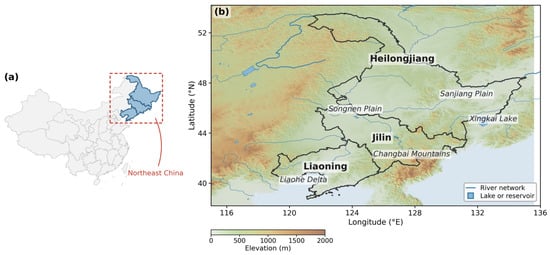
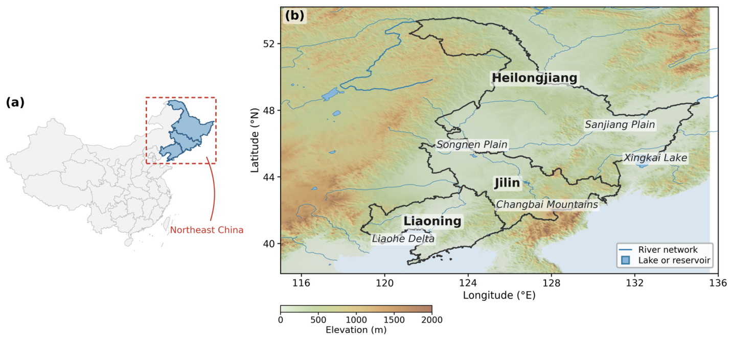
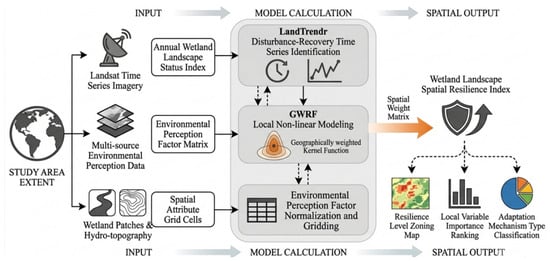
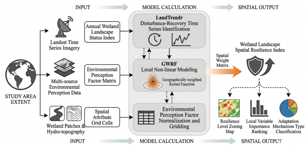
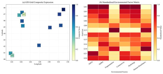
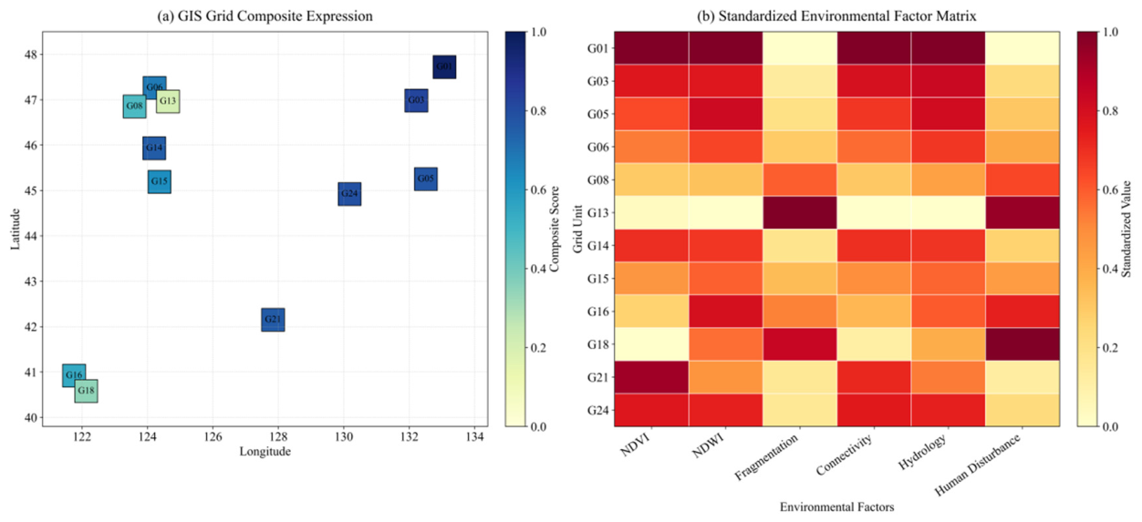
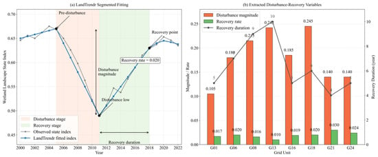
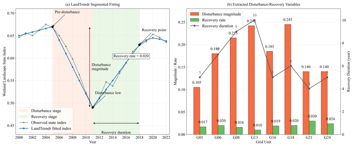
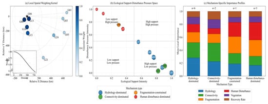
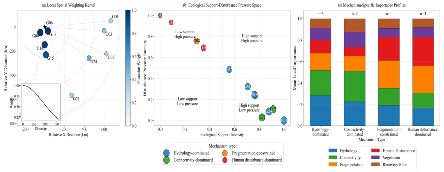
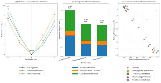
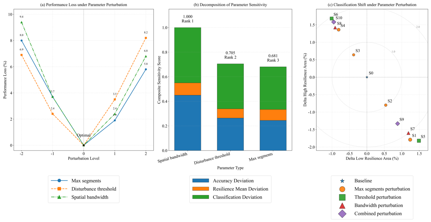
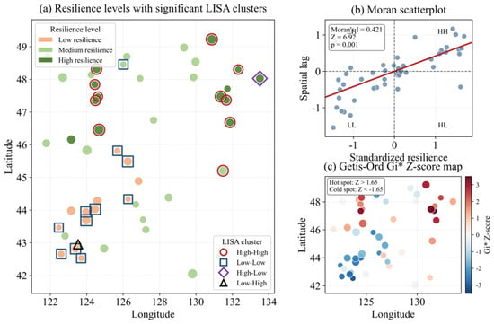
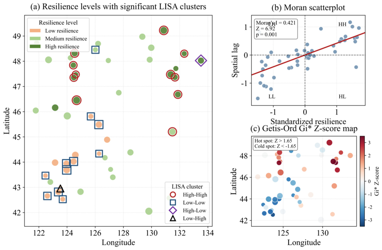
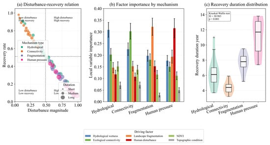
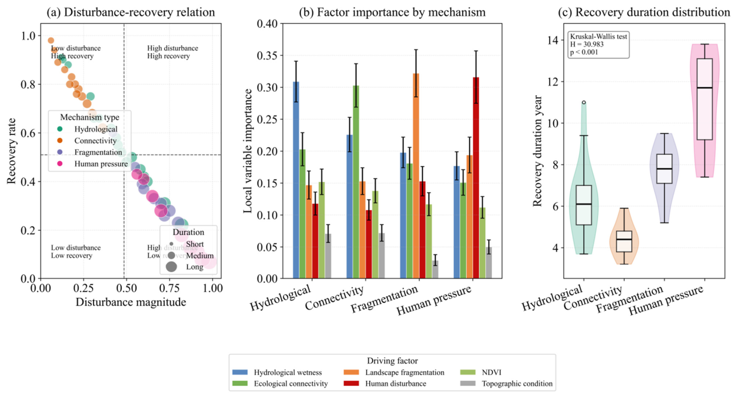

Disclaimer/Publisher’s Note: The statements, opinions and data contained in all publications are solely those of the individual author(s) and contributor(s) and not of MDPI and/or the editor(s). MDPI and/or the editor(s) disclaim responsibility for any injury to people or property resulting from any ideas, methods, instructions or products referred to in the content. |
© 2026 by the authors. Licensee MDPI, Basel, Switzerland. This article is an open access article distributed under the terms and conditions of the Creative Commons Attribution (CC BY) license.