Cross-Configuration 4D DAS-VSP Monitoring for Long-Term CO₂ Storage

Highlights

What are the main findings?

• The main CO₂-related 4D anomaly remained distinguishable in the cross-configuration DAS-VSP comparisons.
• At CRC-4, the combined configuration change was associated with a reduction in anomaly-to-background contrast from 5.0:1 to 3.5:1.

What are the implications of the main findings?

• Maintaining the same sensing configuration remains preferable for long-term monitoring, but planned overlap acquisition can reduce uncertainty when replacement is unavoidable.
• A combined change in DAS sensing configuration, including loss of the original fibre, did not prevent continued time-lapse interpretation in this field case: under the favourable acquisition and signal conditions examined here, the pre-existing baseline remained usable, while redundant fibre paths and backup interrogators can support monitoring continuity.

Abstract

Safe and reliable carbon capture and storage (CCS) requires long-term monitoring to verify secure CO₂ containment. Distributed acoustic sensing vertical seismic profiling (DAS-VSP) provides a practical approach for subsurface monitoring due to its permanent installation, dense spatial sampling, and reduced operational costs. However, monitoring programs spanning decades may require hardware upgrades, including interrogator replacements and changes to fibre-optic cable configurations, affecting time-lapse repeatability and interpretability. This field case study evaluates whether the CO₂-induced 4D DAS-VSP response remains interpretable across a combined change in interrogator, fibre type and optical path, whose individual contributions cannot be isolated. The assessment uses data from the CO2CRC Otway Project Stage 4, where approximately 10 kilotons of CO₂-rich reservoir gas were injected into a saline aquifer at approximately 1500 m depth. Baseline and monitor surveys using different DAS configurations are compared at two monitoring wells, with a same-configuration case as a repeatability benchmark. An established 4D DAS-VSP processing workflow, supplemented by system-specific noise attenuation, is applied to mitigate configuration-dependent differences. The results show that, despite higher non-repeatability, the principal CO₂-related time-lapse anomaly remains spatially localised and distinguishable, indicating that the DAS-VSP response can remain interpretable across a combined configuration change under favourable acquisition and signal-quality conditions.

1. Introduction

Safe and reliable carbon capture and storage (CCS) is critical to meeting global climate objectives and requires demonstrating secure, long-term CO₂ containment. To this end, several large-scale field laboratories have been established worldwide to develop and validate monitoring technologies. The CO2CRC Otway Project in Victoria, Australia, has played an important role in advancing seismic monitoring for geological CO₂ storage. Monitoring the migration of injected CO₂ plumes is essential for verifying storage containment and conformance, as well as for ensuring regulatory requirements [1,2].

Seismic methods are widely used to monitor CO₂ storage projects, with surface seismic surveys commonly used to detect time-lapse differences resulting from CO₂ injection [3,4,5,6,7,8]. However, surface seismic methods pose significant challenges for long-term CCS monitoring, including high operational costs, logistical complexity, land-use disturbance, and limited repeatability due to near-surface variability and changing acquisition conditions [9]. As a result, surface seismic surveys are typically conducted at multi-year intervals, which limits temporal resolution and reduces their effectiveness for operational monitoring [10,11].

These limitations motivate the use of alternative approaches, such as borehole-based vertical seismic profiling (VSP), which is widely applied in CO₂ storage studies and often preferred during the early stages of injection. Compared to surface seismic methods, VSP offers improved signal-to-noise ratio and higher-frequency content near the wellbore, enabling finer-resolution imaging and improved detection of subtle changes (e.g., [7,12,13]).

The introduction of distributed acoustic sensing (DAS) has enhanced the effectiveness of VSP for long-term monitoring by enabling permanent receiver installation, dense spatial sampling along the entire wellbore, and a reduced surface footprint [14,15,16]. Studies have shown that DAS-VSP can produce images comparable to those generated by conventional geophone-based VSP systems [17]. These benefits make DAS-VSP a strong candidate for long-term monitoring, as it offers improved repeatability, lower acquisition costs, and reduced surface disturbance compared to traditional methods [7,14,15,18]. In parallel, field studies have demonstrated that system design choices, including fibre type, can significantly influence signal-to-noise ratio and image quality in DAS-VSP surveys; for example, engineered (scatter-enhanced) fibres have been shown to provide higher signal-to-noise ratio relative to standard telecom fibres (e.g., [19]).

Recent research has expanded the application of DAS-VSP to multi-well and time-lapse monitoring, showing that integrating data from multiple permanently instrumented wells enhances subsurface illumination and sensitivity to CO₂-induced seismic changes [20,21]. Using data from the CO2CRC Otway Project, Pevzner et al. [21] demonstrated that continuous DAS VSP recordings can resolve formation property changes through direct-wave amplitude and traveltime variations: CO₂-induced reductions in formation stiffness and P-wave velocity produced amplitude increases of 15–30% and traveltime delays of 0.3–0.4 ms in the monitored interval. Yurikov et al. [18] further demonstrated that a deterministic processing workflow provides high 4D repeatability and enables recovery of a clear CO₂-related time-lapse signal using an engineered fibre interrogated by a consistent interrogator, and Almukhametova et al. [22] showed consistent results when the same workflow was applied to the Stage 4 surveys.

Field evidence regarding the interpretability of CO₂-induced DAS-VSP responses across such hardware changes remains limited. This study, therefore, assesses time-lapse DAS-VSP performance when the interrogator, fibre type and optical path differ between surveys. The key question is whether the CO₂-induced 4D response remains distinguishable from the increased background non-repeatability introduced by these changes, using an established 4D DAS-VSP workflow supplemented with system-specific noise attenuation.

The CO2CRC Otway Project provides a suitable field case for addressing this question. In Stage 4, approximately 10 kilotons of CO₂-rich reservoir gas were injected into a deep saline aquifer at approximately 1500 m depth via the CRC-3 injection well between November 2024 and January 2025. The monitoring dataset includes simultaneous changes in interrogator, fibre type and optical path under operational field conditions. At CRC-3, damage to the original engineered fibre resulted in a cross-configuration baseline–monitor dataset, whereas at CRC-4, both same- and cross-configuration comparisons are available. These complementary datasets allow the effect of the combined configuration change on repeatability to be assessed while testing whether the principal CO₂-related 4D response remains distinguishable from the resulting non-repeatability background.

2. Data Acquisition

The CO2CRC Otway Project is organized into sequential stages, each representing a distinct phase of monitoring and technological advancement. Stage 3 included the M8 DAS-VSP survey in March 2021, which serves as the baseline dataset for this study. The final approximately 2.5 kt of the Stage 3 injection was completed after this survey [18]. Stage 4 was subsequently implemented, incorporating the reperforation of CRC-3 [22], changes to the interrogator and fibre configuration and the injection of approximately 10 kilotons of CO₂-rich reservoir gas between November 2024 and January 2025. The subsequent M9 DAS-VSP survey, acquired in February 2025 after completion of Stage 4 injection, provides the monitoring dataset for time-lapse analysis. Both surveys employed consistent acquisition geometries to enable a reliable assessment of reservoir changes.

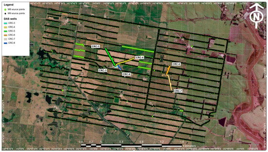
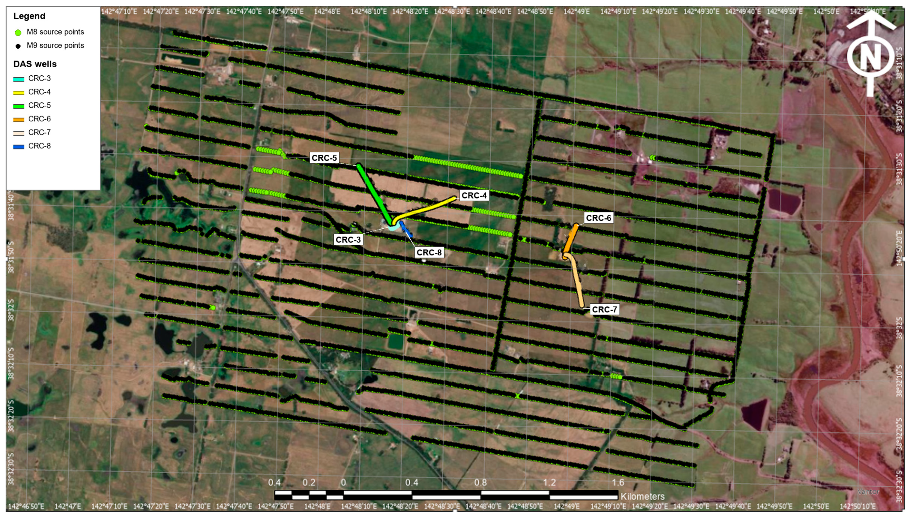
The M8 and M9 surveys were designed with consistent acquisition geometries, employing surface seismic sources positioned along predefined source lines that match those used in previous Otway stages [18,20]. More than 96% of the M8 source locations were reoccupied and reshot during the M9 survey (Figure 1). Minor gaps in M9 coverage were due to temporary access restrictions but did not affect the overall offset or azimuthal distribution. Source-sweep parameters and acquisition geometry remained consistent, with a median horizontal source repositioning of 0.11 m (91% of shots within 1 m) and a median elevation difference of 0.14 m (Supplementary Figure S1). Data acquisition utilized an INOVA UniVib (INOVA Geophysical, Sugar Land, TX, USA) seismic source (116 kN peak force) with a linear sweep from 6 to 150 Hz over 24 s, with a 0.5 s cosine taper.

Figure 1. Map of the CO2CRC Otway Stage 4 survey area showing the M8 baseline (green) and M9 monitor (black) source locations and the surface projections of the DAS wells CRC-3 through CRC-8. More than 96% of the M8 source locations were reoccupied in M9; green points without black symbols mark locations occupied only in M8. Coordinates are geographic (latitude and longitude); background imagery: Vantor.

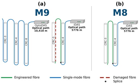
During the M9 survey, DAS-VSP monitoring was conducted in wells CRC-3 through CRC-8 (Figure 1). CRC-3 is a vertical injection well, while wells CRC-4 through CRC-8 are deviated monitoring wells that provide lateral coverage of the reservoir. This study examines time-lapse performance across configurations that differ in fibre installation, interrogator, and optical path, as summarized schematically for the M8 and M9 surveys in Figure 2 and Table 1. Wells CRC-5, CRC-6, and CRC-7 are excluded from further analysis in this study because their fibre and interrogator configurations remained unchanged between M8 and M9. CRC-8 is also excluded because it lacks a baseline dataset, as it was drilled after the M8 survey. As a result, the analysis focuses on CRC-4 and CRC-3, which represent the range of interrogator, fibre, and optical-path changes observed in the Otway datasets.

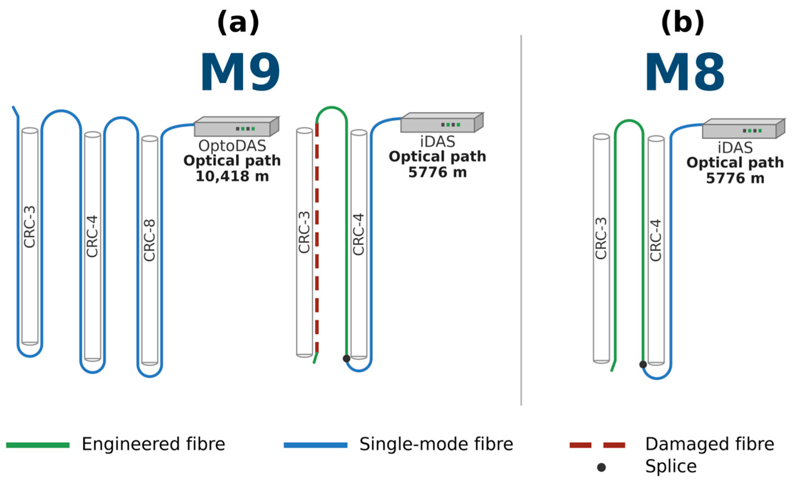
Figure 2. DAS interrogator and fibre configurations at CRC-3 and CRC-4 for the M9 monitor survey (a) and M8 baseline survey (b). Fibre types are indicated by colour, with engineered fibre shown in green, single-mode fibre in blue, and damaged fibre sections by dashed brown lines. The schematic also shows the interrogator used for each survey and the corresponding optical routing through the monitored wells, and the optical path length of each configuration is annotated; dots mark the splice between the single-mode lead-in and the engineered fibre in CRC-4.

Table 1. DAS interrogator, fibre configurations, and recording parameters for the M8 baseline and M9 monitoring DAS-VSP surveys at the CO2CRC Otway Project.

Parameter	M8 iDAS (Baseline)	M9 iDAS (Monitor 1)	M9 OptoDAS (Monitor 2)
DAS interrogator	Silixa iDAS	Silixa iDAS	ASN OptoDAS
Fibre type	CF	CF	SMF
Channel spacing	1.0 m	1.0 m	1.02 m
Gauge length	10.0 m	10.0 m	10.21 m
Temporal sampling rate	1000 Hz	1000 Hz	1000 Hz
Optical path length	5776 m	5776 m	10,418 m
Instrumented wells	CRC-3, CRC-4	CRC-3 †, CRC-4	CRC-8, CRC-4, CRC-3

† CF damaged at CRC-3 during M9; no usable data acquired.

The M9 DAS-VSP survey was acquired using a dual-interrogator setup, with the ASN OptoDAS (Alcatel Submarine Networks Norway AS, Trondheim, Norway) interrogator deployed as a backup to the primary Silixa iDAS-v3 P06 (Silixa Ltd., Elstree, UK). This allowed two sensing configurations to be compared under identical acquisition and source conditions, although the configurations differ in more than one component: engineered Constellation Fibre (Silixa Ltd., Elstree, UK). recorded with iDAS, and standard single-mode fibre (SMF) recorded with OptoDAS. The optical layouts differed significantly. The iDAS configuration followed a hybrid path: an SMF lead-in in CRC-4 spliced to CF at depth, continuing to the CF cemented behind casing in CRC-3; the SMF lead-in only transmitted the light, and all iDAS recordings were made on the CF. In contrast, the OptoDAS configuration used a continuous SMF loop passing sequentially through CRC-8, CRC-4, and CRC-3 in a down-and-up configuration. This resulted in a substantially longer optical path for OptoDAS (10,418 m at CRC-3) than for iDAS (5776 m), corresponding to about 1.9 dB of additional two-way optical loss for a typical single-mode fibre attenuation of 0.2 dB/km [23].

At CRC-4, both systems operated simultaneously, allowing a direct cross-configuration comparison along the same well trajectory. At CRC-3, however, the engineered CF was damaged during reperforation due to fluid ingress, rendering the iDAS recordings unusable. The SMF used by OptoDAS remained intact because it terminated above the reservoir interval. As a result, OptoDAS provided the only viable DAS data at CRC-3 for the M9 survey. Because the interrogator, fibre type, and optical path changed together, their individual contributions cannot be isolated from these data (Section 5.3). Hereafter, configuration change refers to this combined change, and the labels “same-configuration” and “cross-configuration” identify the comparisons without implying that any single component is isolated.

3. Data Processing Workflow

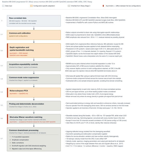
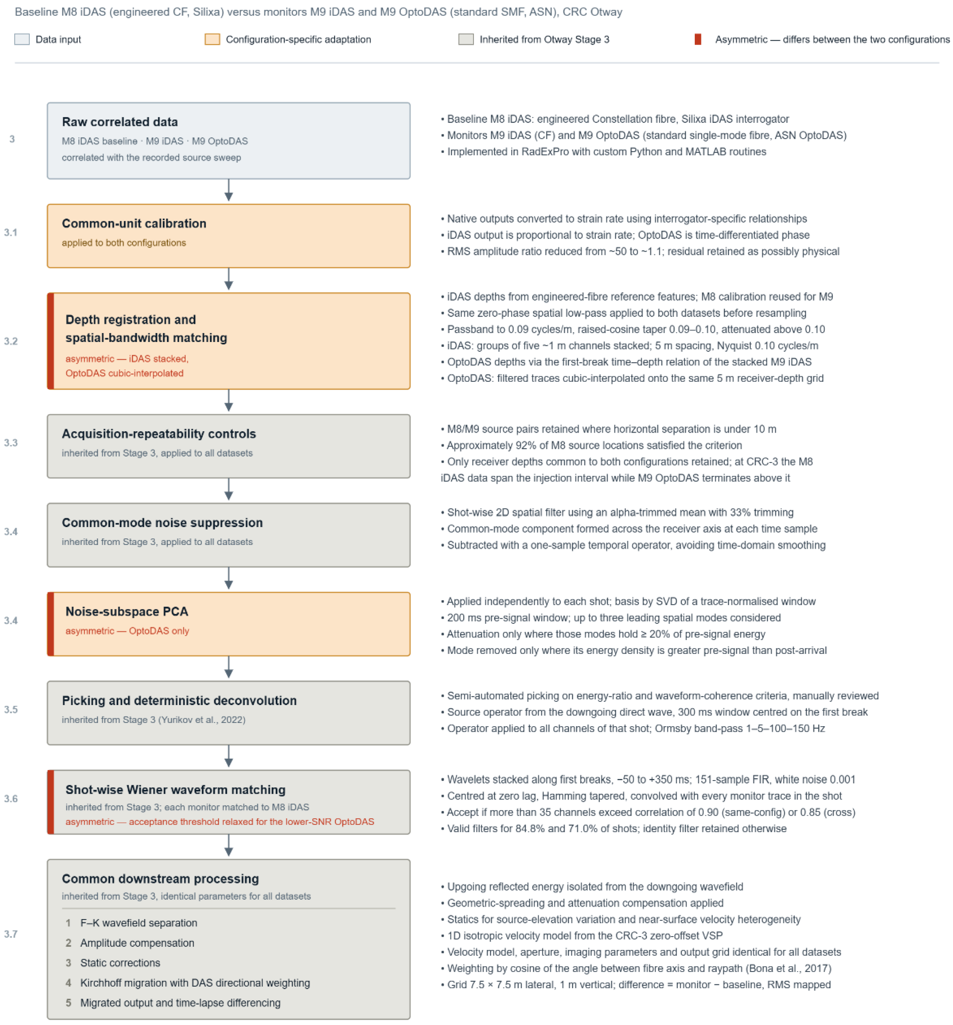
The DAS-VSP processing applied in this study builds on the workflow established during Otway Stage 3 [18,20]. For the present field case, configuration-specific adaptations were introduced to address differences in amplitude scaling, channel-depth correspondence, spatial bandwidth, noise characteristics, and waveform response between the iDAS and OptoDAS datasets. Processing steps inherited unchanged from the Stage 3 workflow are summarized, whereas the configuration-specific adaptations and their quality-control criteria are described in greater detail. The complete workflow is presented in Figure 3.

Figure 3. Processing workflow applied to the M8 and M9 DAS-VSP datasets for same- and cross-configuration time-lapse analysis. Grey boxes indicate processing steps inherited from the Otway Stage 3 workflow [18,20], orange boxes indicate configuration-specific adaptations, and the light-blue box denotes the input data. Red side markers identify steps that differ between the two sensing configurations. Section numbers shown on the left refer to the corresponding manuscript sections. PCA was applied only to the OptoDAS data; an iDAS control test is reported in Section 5.1.

In this study, iDAS denotes datasets acquired using engineered Constellation Fibre (CF) interrogated by a Silixa iDAS interrogator. In contrast, OptoDAS denotes datasets acquired using standard single-mode fibre (SMF) interrogated by an ASN OptoDAS interrogator. The M8 survey serves as the baseline, and the M9 survey serves as the monitor. Processing was implemented using RadExPro Professional 2024.4, custom Python scripts (Python 3.12.7), and MATLAB R2025a (version 25.1).

Three major adaptations were introduced to the established Otway Stage 3 processing workflow for the cross-configuration comparison: conversion to common strain-rate units; channel-depth registration and spatial-bandwidth matching; and additional attenuation of the stronger coherent and background noise present in the OptoDAS recordings. The remaining processing followed the established Stage 3 workflow.

3.1. Common-Unit Calibration

After correlation with the source sweep, the raw iDAS and OptoDAS measurements were converted from their native output scales to strain rate using interrogator-specific calibration relationships. This step was required for the cross-configuration comparison because the two interrogators provide different native outputs and scaling conventions. The iDAS output is proportional to strain rate, whereas the OptoDAS output represents time-differentiated optical phase.

Before conversion, the RMS amplitudes differed by a factor of approximately 50. After conversion to strain rate, the RMS-amplitude ratio was reduced to approximately 1.1, confirming that most of the initial amplitude discrepancy resulted from the different native scaling conventions. The remaining difference was retained because it may reflect genuine configuration-dependent effects.

3.2. Channel-Depth Registration and Spatial-Bandwidth Matching

The iDAS and OptoDAS datasets differed in channel-depth coordinates and effective spatial sampling. The M8 iDAS depths were calibrated using known engineered-fibre reference features, and the same calibration was applied to the M9 iDAS, as the fibre installation was unchanged.

Although recorded at approximately 1 m spacing, groups of five adjacent iDAS channels contained nearly identical measurements. Each non-overlapping group was therefore stacked into a single representative trace. This 5 m independent spacing corresponds to a spatial Nyquist wavenumber of 0.10 cycles/m and defines the upper limit of the common spatial bandwidth used for comparison.

Both datasets were filtered along the channel axis using the same zero-phase spatial low-pass filter before resampling. Wavenumbers up to 0.09 cycles/m were preserved, a raised-cosine taper was applied between 0.09 and 0.10 cycles/m, and energy above 0.10 cycles/m was removed. The iDAS stacks were retained on the resulting 5 m grid. For the OptoDAS dataset, channel depths were determined using the first-break time–depth relationship derived from the depth-calibrated M9 iDAS data after stacking onto the 5 m grid. OptoDAS first-break times were mapped through this relationship to assign the corresponding receiver depths. The filtered OptoDAS data were then resampled by cubic interpolation onto the same 5 m receiver-depth grid as the iDAS data.

This procedure established common receiver depths and spatial bandwidths for comparison, reducing cross-configuration differences arising from unequal channel coordinates, depth coverage, and spatial sampling. The small differences in gauge length (10.0 versus 10.21 m) and channel spacing (1.0 versus 1.02 m) were not compensated explicitly. For the P-wave signal, the gauge-length difference changes the theoretical strain-rate response by about 1% or less [24], estimated for P-wave velocities of 2.4–3.2 km/s, and the channel-spacing difference is accommodated by the first-break-based depth assignment and the common 5 m grid.

3.3. Acquisition-Repeatability Controls

Common source locations were matched between the M8 and M9 surveys using a maximum horizontal separation of 10 m, retaining approximately 94% of the M8 sources. Only receiver depths common to both configurations were included in the comparison. The receiver-depth restriction was particularly important at CRC-3, where the M8 iDAS data extended across the injection interval, whereas the M9 OptoDAS data terminated above the reservoir.

Time-lapse repeatability was quantified using the standard normalised root-mean-square difference (NRMS) of the baseline and monitor traces, following [25]:

$$\mathrm{NRMS}=200\times {\displaystyle \frac{\mathrm{RMS}(m-b)}{\mathrm{RMS}\left(m\right)+\mathrm{RMS}\left(b\right)}}$$

(1)

where b and m are the baseline and monitor traces within the analysis window, and RMS is the root-mean-square amplitude over the samples of the window. For the shot-gather analysis, NRMS was calculated within a fixed 60 ms window. Identical windows and depth intervals were used for the same and cross-configuration comparisons.

NRMS was used as a quality-control measure throughout the processing sequence to track changes in repeatability after noise attenuation, deconvolution, and waveform matching. It was not used to control shot rejection or to modify the processed data.

3.4. Noise Attenuation

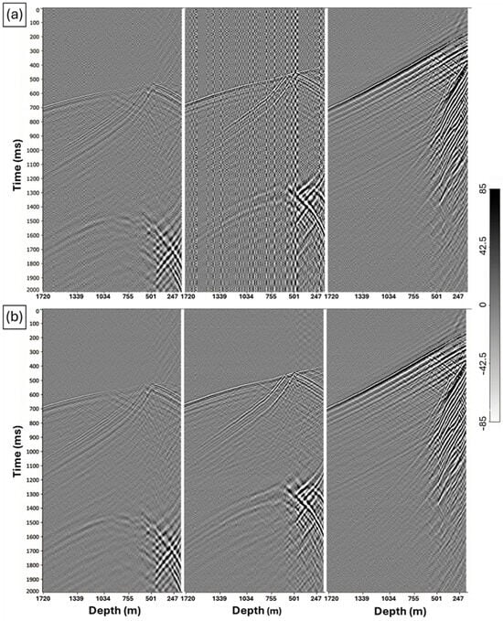
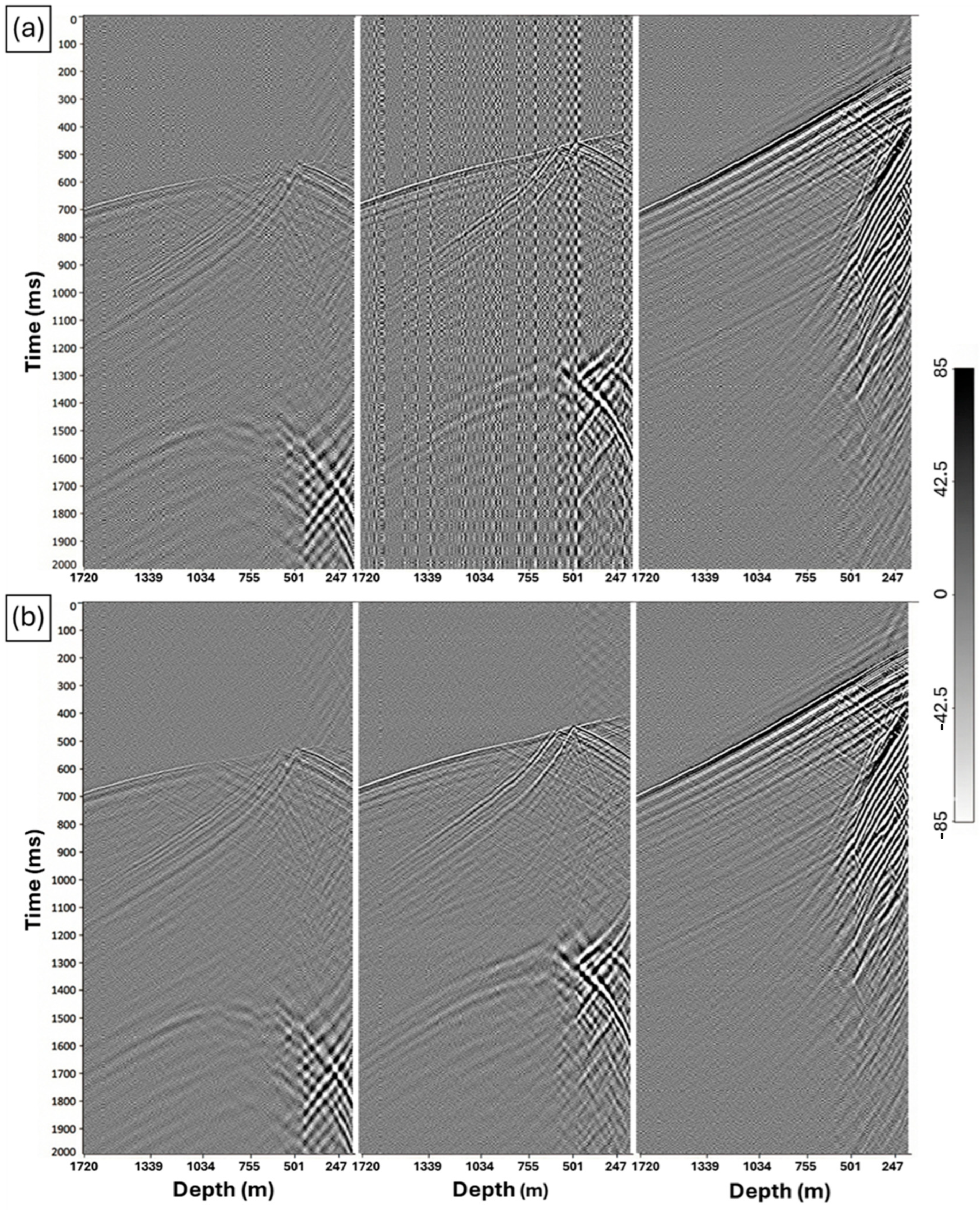
Noise was one of the main differences between the datasets, with the OptoDAS gathers showing higher levels of stripe-type and background noise (Figure 4a). The noise amplitude and spatial structure varied between shots. We therefore adapted the attenuation separately for each shot. Noise attenuation was applied in two stages: a common spatial filter for both datasets, followed by an additional principal component analysis (PCA) filter for the OptoDAS data.

Figure 4. Representative CRC-4 OptoDAS shot gathers showing shot-to-shot variability in noise character and intensity: (a) before noise attenuation, where the level and spatial distribution of noise differ markedly between source points, and (b) after adaptive, conservative attenuation, which reduces the dominant noise while preserving coherent seismic arrivals.

A shot-wise 2D alpha-trimmed mean filter was first applied to both iDAS and OptoDAS gathers. At each time sample, amplitudes across receiver channels were sorted. A total of 33% of the samples was discarded symmetrically from the two tails, and the trimmed mean was calculated from the remaining samples. This common-mode component was subtracted from every receiver channel at that time sample. No time-domain smoothing was applied. This produced only minor changes in the iDAS data but stronger attenuation of the stripe-type noise in the OptoDAS recordings.

Residual noise in the OptoDAS data was attenuated using a shot-wise noise-subspace PCA workflow. For each shot, a spatial noise basis was estimated by applying singular value decomposition (SVD) to a trace-wise RMS-normalised 200 ms pre-first-break window. Up to three leading spatial modes were identified, and PCA attenuation was applied only when these modes together represented at least 20% of the pre-signal energy. Because PCA was applied only to the OptoDAS data, the same workflow was also applied to the iDAS data as a control (Section 5.1).

To minimise the removal of seismic signal, each candidate mode was projected onto the full RMS-normalised gather along the receiver axis. The coefficient series was analysed in two windows: the pre-signal window and a 350 ms post-arrival window starting at the first break. A mode was classified as noise and removed only when its mean-squared coefficient energy was higher before the first break than after it (energy ratio < 1). Otherwise, the mode was retained. A maximum of three modes could be removed from any shot.

The selected noise modes were reconstructed and subtracted from the normalised gather, after which the original trace amplitudes were restored. The removed components were visually inspected to ensure that coherent seismic events were preserved. Figure 4b illustrates the corresponding improvement after the OptoDAS-specific noise attenuation. Performance was assessed using pre-arrival noise reduction, event continuity, first-arrival signal-to-noise ratio (SNR), waveform correlation, and NRMS.

3.5. First-Break Picking and Deterministic Deconvolution

First-break picking followed the semi-automated workflow for Otway Stage 3 by [18,20]. Initial picks based on energy-ratio and waveform-coherence criteria were visually reviewed and manually corrected where required.

For each shot, a deterministic deconvolution operator was estimated from the downgoing direct wave within a 300 ms window centred on the first break and applied to all receiver channels. The deconvolved data were then band-pass filtered with Ormsby operators (0–40–80–160 Hz and 5–10–90–180 Hz).

This established step compressed the source wavelet and reduced spectral and wavelet-duration differences before waveform matching. Its effect was assessed from direct-wave compression and changes in NRMS.

3.6. Shot-Wise Wiener Waveform Matching

Residual differences in amplitude, phase, and wavelet shape remained between the M8 baseline and M9 monitor data after the preceding processing. Shot-wise Wiener filters were therefore estimated independently for the M9 iDAS and M9 OptoDAS datasets, using the corresponding M8 iDAS data as the reference.

For each shot, baseline and monitor wavelets were extracted along the first-break trajectory from −50 to +350 ms relative to the picks and stacked over all picked receiver channels with a 30% trimmed mean. A 151-sample finite-impulse-response Wiener filter was estimated to transform the monitor wavelet into the baseline wavelet. The solution used a white-noise stabilisation factor of 0.001, was centred at zero lag, tapered with a Hamming window, and convolved with every monitor trace in that shot, so that the same operator applies at all receiver depths.

Before filter estimation, baseline–monitor correlation was evaluated for individual receiver channels after applying an Ormsby band-pass filter with corner frequencies of 6–10–50–100 Hz, used for this evaluation only, and allowing a maximum relative lag of 5 ms. A filter was accepted only when more than 40 channels exceeded a minimum correlation of 0.90, for both the same-configuration M8 iDAS–M9 iDAS and the cross-configuration M8 iDAS–M9 OptoDAS comparisons. Shots that did not satisfy these criteria were rejected from the waveform-matched analysis and were not used in the subsequent repeatability assessment or migrated time-lapse comparison. All other filter parameters were identical in the two cases.

The accepted filters were used to reduce residual waveform differences between the baseline and monitor datasets. For the same-vintage M9 iDAS–M9 OptoDAS comparison, the corresponding processed M9 datasets after their respective M8-referenced waveform matching were compared directly, providing an assessment of the residual cross-configuration mismatch under common acquisition conditions. Performance was evaluated using changes in waveform correlation and NRMS, with the same-configuration M8–M9 result serving as the repeatability benchmark.

3.7. Established Downstream Processing

Following waveform matching, all datasets were processed using the established Otway Stage 3 workflow without further configuration-specific modification [18,26]. The sequence included F–K wavefield separation, amplitude compensation, static corrections for source-elevation and near-surface variations, and Kirchhoff migration using a 1D isotropic velocity model derived from the CRC-3 zero-offset VSP.

The same velocity model, migration aperture, imaging parameters, and output grid were used for all baseline and monitor datasets. Migration also included DAS directional-sensitivity weighting based on the angle between the fibre axis and the ray path, following Bona et al. [27].

The migrated volumes were output on a regular 3D grid with 7.5 m × 7.5 m lateral spacing and 2 m vertical sampling. Time-lapse difference volumes were generated by subtracting the migrated baseline volume from the corresponding monitor volume.

4. Results

4.1. Raw Data Comparison

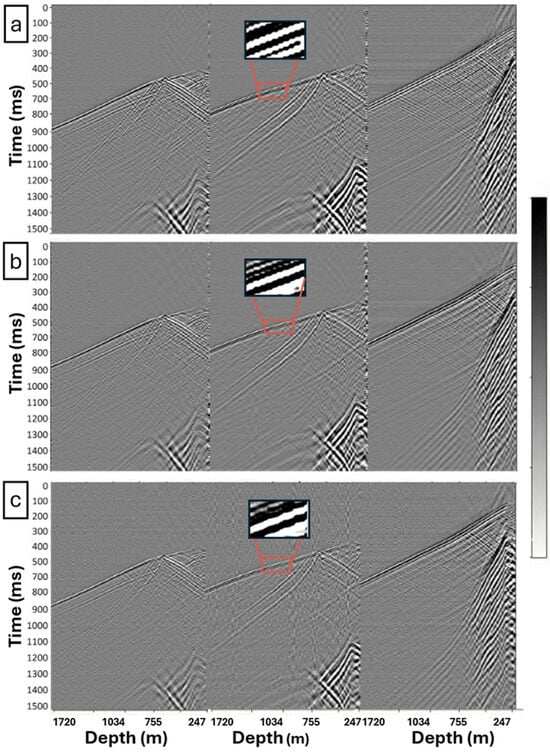
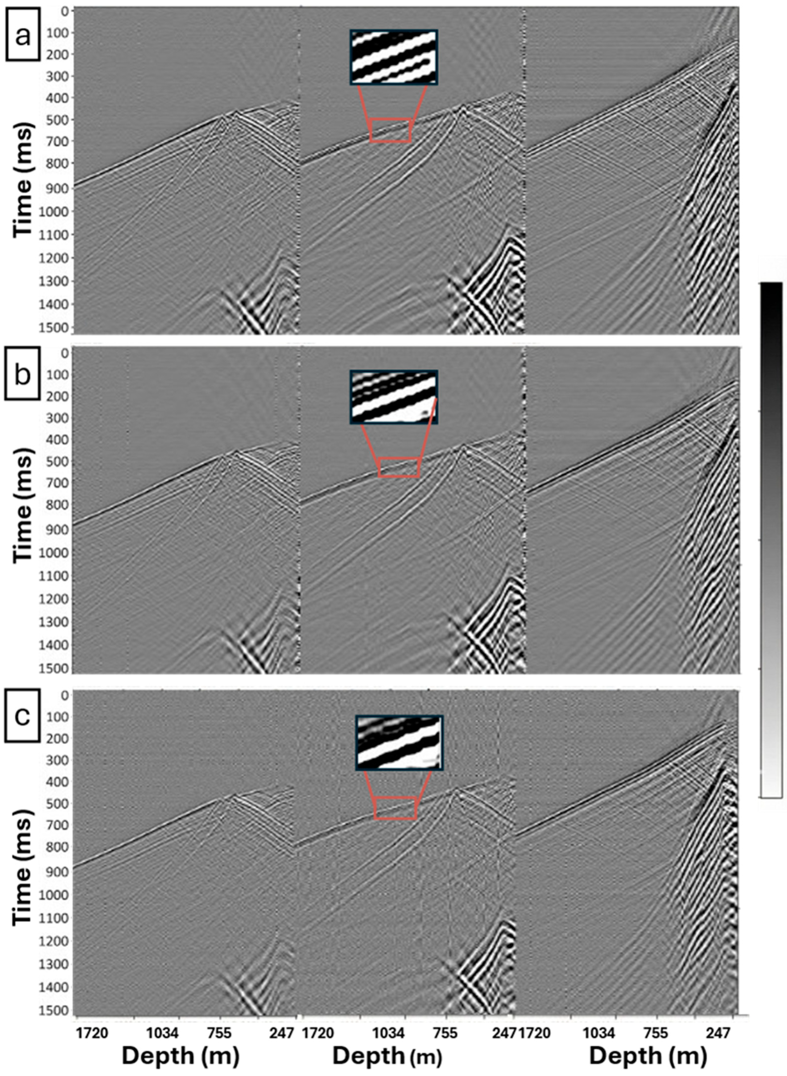
Figure 5a–c present representative DAS-VSP shot gathers from the Otway Stage-4 surveys. These figures compare the baseline M8 iDAS dataset (Figure 5a), the monitor M9 iDAS dataset (Figure 5b), and the monitor M9 OptoDAS dataset (Figure 5c). All three gathers are displayed after channel-depth registration to provide a common depth reference; no denoising, spatial-bandwidth matching, deconvolution, or waveform matching has been applied.

Figure 5. Comparison of representative DAS shot gathers from the CRC-4 well acquired during different surveys and fibre configurations. (a) Shot gathers from the M8 iDAS survey recorded on engineered-backscatter fibre (baseline reference). (b) Shot gathers from the M9 iDAS survey recorded on the same engineered-backscatter fibre. (c) Shot gathers from the M9 OptoDAS survey recorded on a single-mode fibre. In each panel, the three columns correspond to near-, mid-, and far-offset shots, respectively. Within each panel, all shots share a common amplitude scale, while each panel is independently scaled to its own maximum amplitude. The red boxes mark a representative window around the downgoing arrival highlighting waveform character.

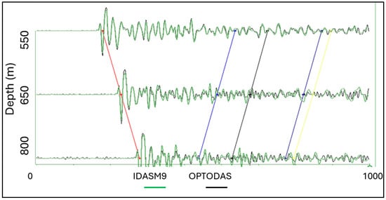
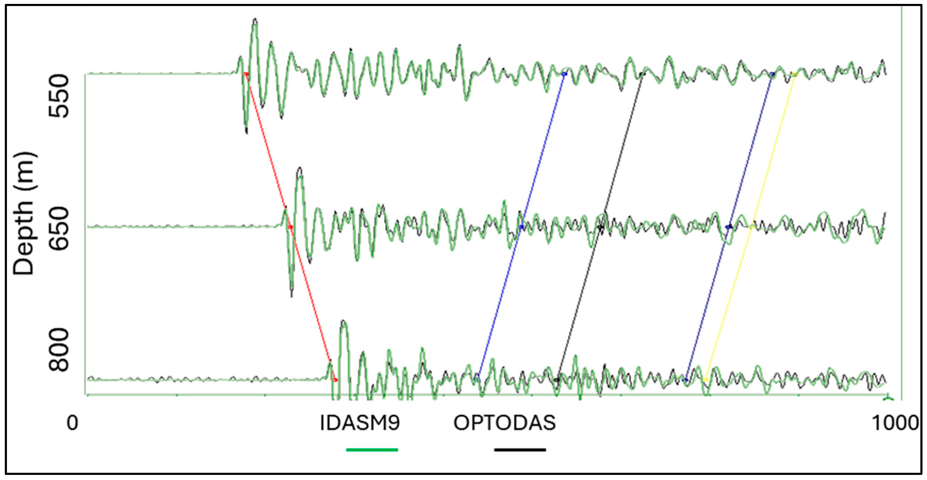
Figure 5 shows raw data before common-unit calibration (Section 3.1); each panel is therefore scaled to its own maximum, and the panels are compared for kinematics and wavefield character rather than amplitude. The baseline and monitor iDAS datasets (Figure 5a,b) display similar downgoing and upgoing wavefield characteristics. This strong correspondence is consistent with good baseline–monitor repeatability for the same configuration. In contrast, the OptoDAS monitor data retains the overall kinematic structure but shows a strong vertical striping, which reduces event continuity and obscures reflected energy. Despite these differences in data quality, the downgoing and upgoing kinematics remain consistent across all three datasets. No systematic time stretching or compression is observed. Figure 6 further illustrates this by comparing three overlaid traces from the M9 iDAS and M9 OptoDAS datasets at depths of 800 m, 650 m, and 550 m. For each channel, five representative events were picked to enable direct comparison of arrival times. The corresponding arrivals are closely aligned, with no systematic arrival-time shift evident between the two configurations.

Figure 6. Zoomed comparison of overlaid, amplitude-normalised wiggle traces from the M9 iDAS (green) and M9 OptoDAS (black) datasets at depths of 800 m, 650 m, and 550 m. The red marker highlights the first downgoing arrival, while the remaining colored markers track representative upgoing reflection events at later times. Across all depths, the corresponding events exhibit close temporal alignment, with no measurable shift within sampling precision between the two configurations.

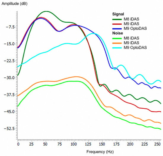
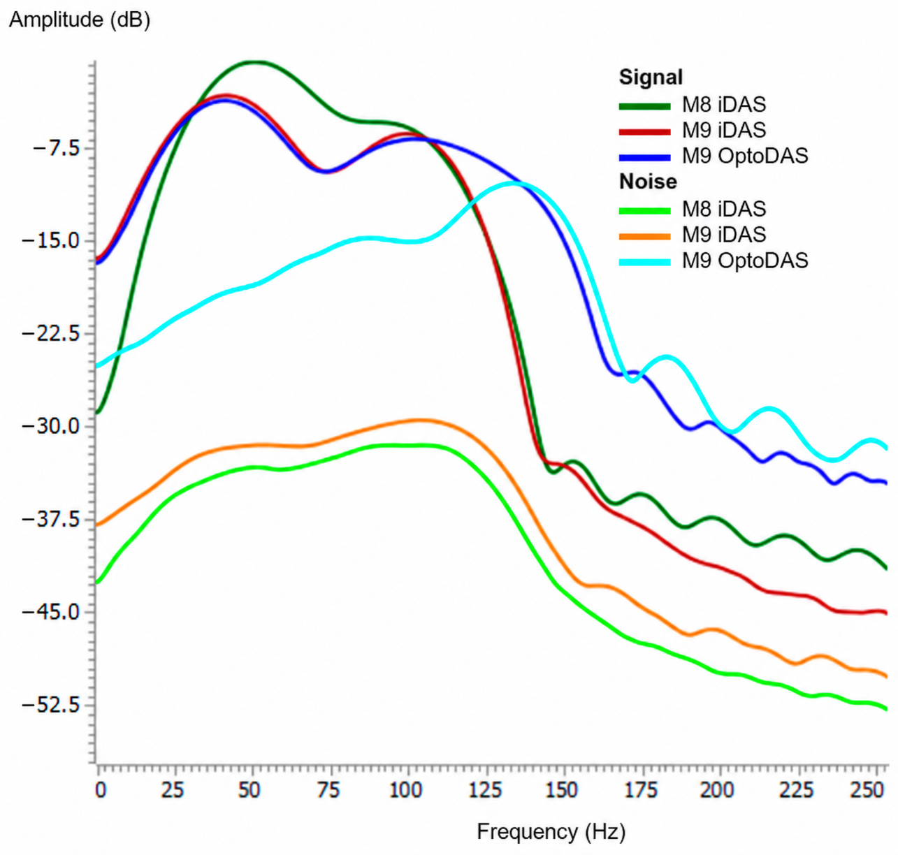
The amplitude spectra in Figure 7 were computed from the three representative shot gathers shown in Figure 5 using a 60 ms signal window centred on the picked first-arrival P-wave and a separate 60 ms pre-arrival noise window immediately preceding it, averaging over receiver depths from 700 to 1400 m. All six spectra are referenced to the maximum of the M8 iDAS signal spectrum so that both the spectral shape and the relative level can be compared. Most of the coherent signal energy lies between approximately 20 and 120 Hz. The M9 iDAS and M9 OptoDAS signal-window spectra are closely comparable below approximately 105 Hz, generally differing by less than about 1 dB. Above approximately 105–110 Hz, however, the OptoDAS signal-window spectrum remains progressively higher than the M9 iDAS spectrum while its corresponding noise spectrum rises toward the signal level, indicating an increasing contribution of noise to the measured high-frequency energy. In contrast, the M8 iDAS signal spectrum contains proportionally less energy below approximately 25 Hz and peaks near 50 Hz, compared with approximately 40 Hz for the M9 datasets.

Figure 7. Amplitude spectra of DAS-VSP data for the baseline M8 iDAS survey and the M9 iDAS and M9 OptoDAS monitor surveys. Signal spectra were computed using a 60 ms window centered on the picked first-arrival P-wave, and noise spectra from a 60 ms pre-arrival window immediately preceding it, both averaged over receiver depths from 700 to 1400 m. All spectra are referenced to the maximum of the M8 iDAS signal spectrum (0 dB) so that spectral shape and relative level can be compared between datasets. The spectra illustrate differences in signal bandwidth and noise level between the two interrogator–fibre configurations across the frequency range of interest.

The clearest difference is in the noise spectra. The M8 and M9 iDAS noise levels remain approximately 30 dB below their respective signal maxima over much of the analysed band. In contrast, the OptoDAS noise spectrum is approximately 13–16 dB higher than the iDAS noise spectra over approximately 20–105 Hz and rises further relative to the signal at higher frequencies. At the main signal peak, the signal-to-noise separation is approximately 29 dB for M9 iDAS and 16 dB for M9 OptoDAS. The OptoDAS signal-to-noise separation progressively decreases with frequency and approaches zero near 135–140 Hz, where the signal- and noise-window spectra converge. The apparent persistence of OptoDAS energy above approximately 110 Hz therefore largely reflects increasing contamination of the signal window by the elevated noise floor rather than additional coherent seismic bandwidth.

4.2. CRC-4 and CRC-3 Repeatability Analysis

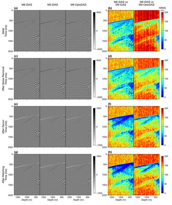
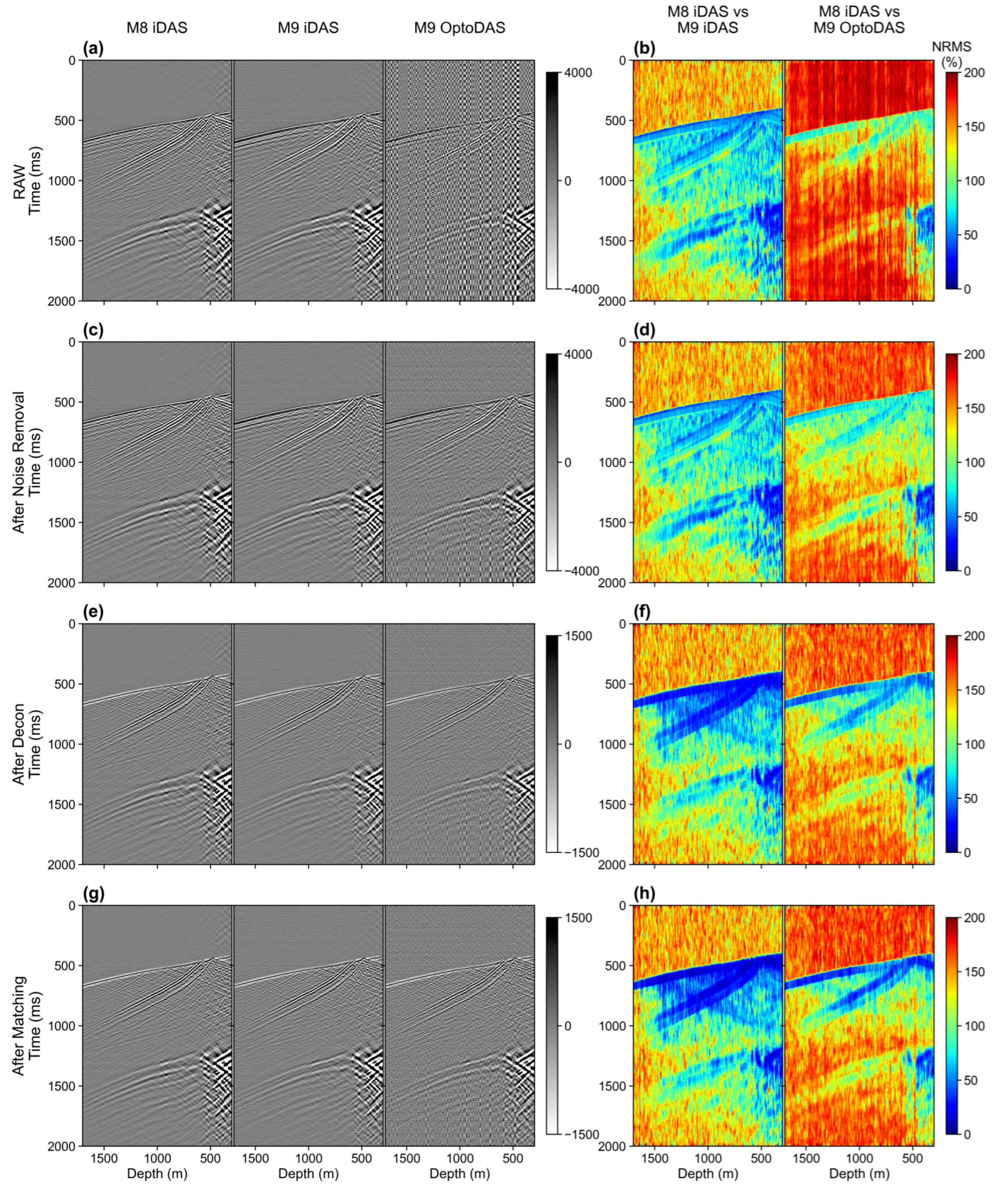
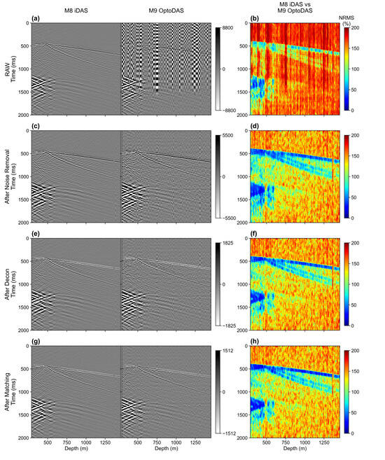
Figure 8, Figure 9 and Figure 10 evaluate how the main processing stages affect agreement between the DAS datasets at CRC-4 and CRC-3. At CRC-4, the M8 iDAS–M9 iDAS comparison provides the same-configuration baseline–monitor reference, while the M8 iDAS–M9 OptoDAS comparison represents the cross-configuration time-lapse case. Figure 10 additionally includes the same-vintage M9 iDAS–M9 OptoDAS comparison, which provides a direct constraint on cross-configuration mismatch without the M8–M9 survey interval. At CRC-3, only the M8 iDAS–M9 OptoDAS cross-configuration comparison is available because the main sensing cable was damaged during reperforation due to fluid ingress prior to the Stage 4 monitor survey. Throughout this section, the pre-denoising reference state is the matched data: the gathers after common-unit calibration, channel-depth registration, common receiver selection, and spatial-bandwidth matching, but before noise attenuation, deconvolution, and waveform matching.

Figure 8. Representative CRC-4 shot gathers (left column; (a,c,e,g)) and the corresponding trace-by-trace NRMS (right column; (b,d,f,h)) at successive processing stages, one stage per row: (a,b) matched pre-denoising data, (c,d) after noise attenuation, (e,f) after deconvolution, and (g,h) after shot-wise Wiener matching. Each gather panel shows, from left to right, the M8 iDAS baseline, the M9 iDAS monitor, and the M9 OptoDAS monitor for the same source. Each NRMS panel shows, from left to right, the same-configuration M8 iDAS–M9 iDAS and the cross-configuration M8 iDAS–M9 OptoDAS comparison over the full receiver-depth range, calculated at each trace using a 60 ms window, on a 0–200% colour scale.

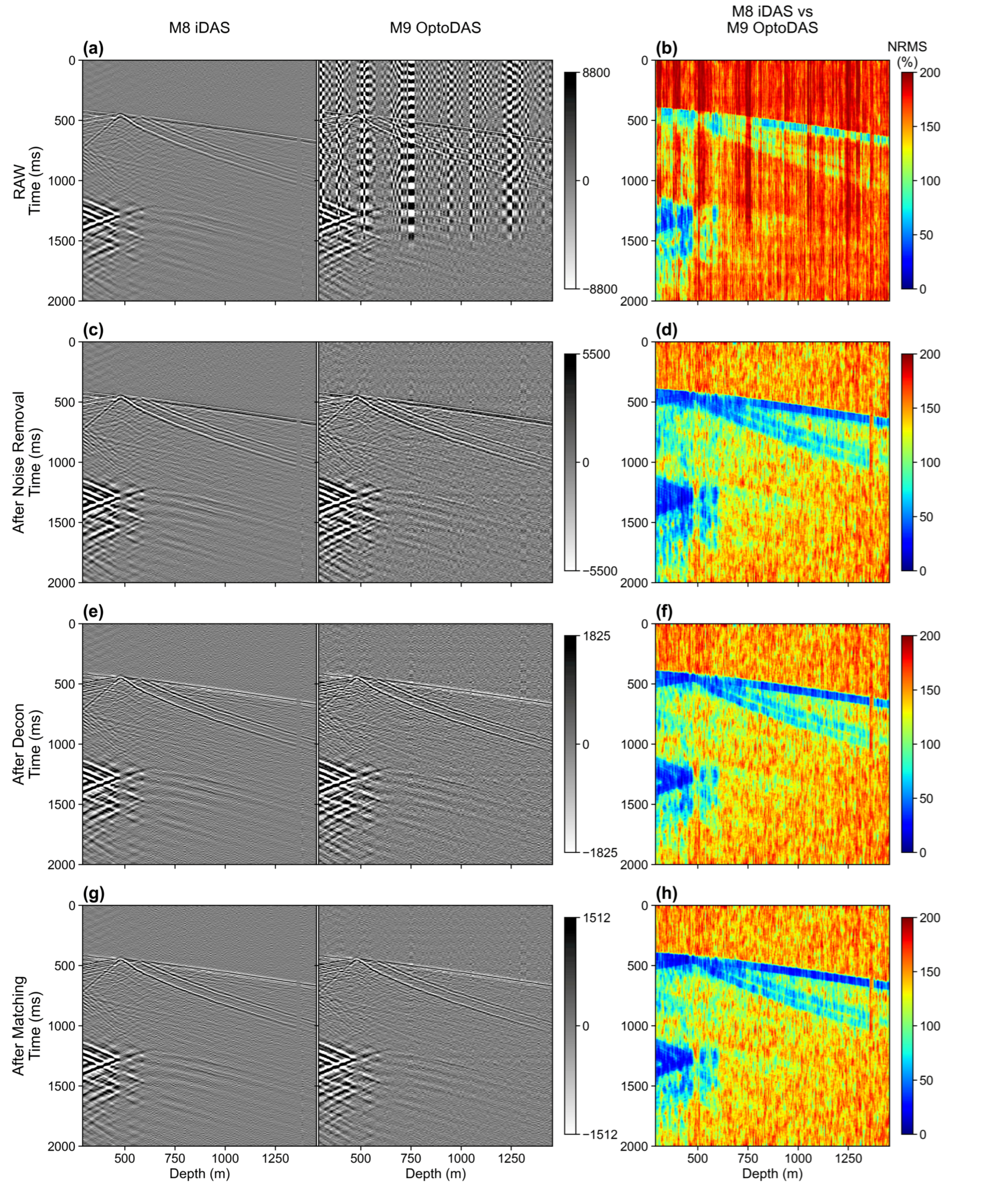
Figure 9. CRC-3 cross-configuration comparison (M8 iDAS baseline versus M9 OptoDAS monitor) shown through successive processing stages. Left panels display the shot gathers for M8 iDAS and M9 OptoDAS, and right panels show NRMS along the full receiver-depth range, calculated at each trace using a 60 ms window. Rows correspond to the matched pre-denoising data (a,b), after noise attenuation (c,d), after deterministic deconvolution (e,f), and after shot-wise Wiener matching (g,h).

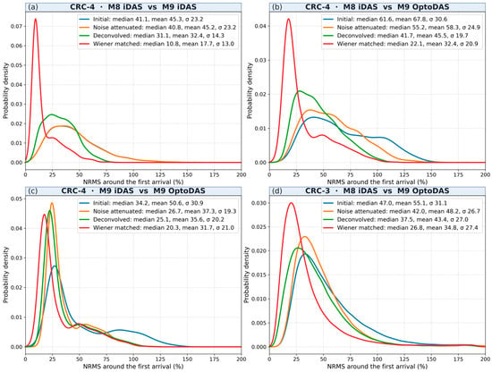
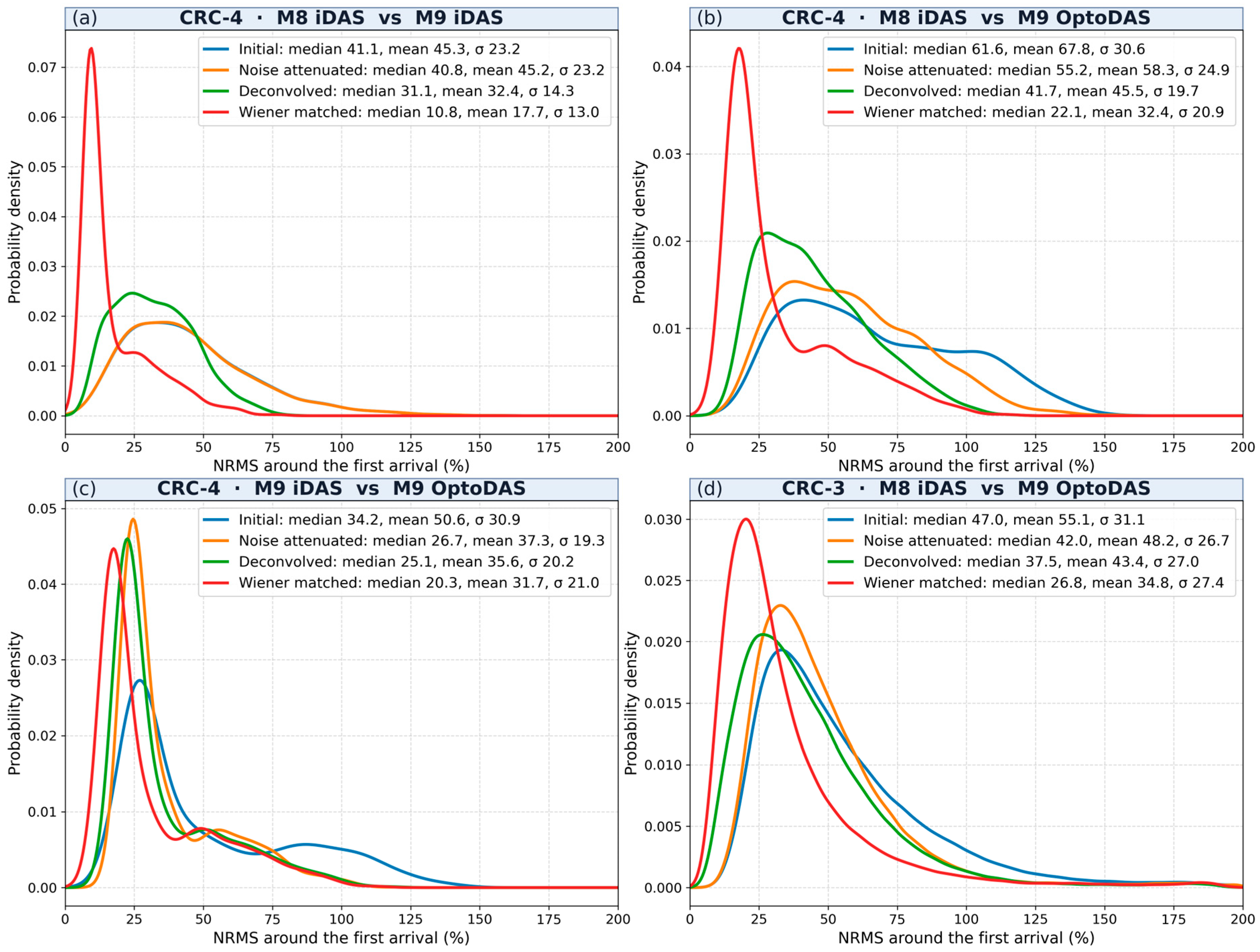
Figure 10. NRMS distributions calculated around the first arrival for (a) the CRC-4 same-configuration comparison (M8 iDAS–M9 iDAS), (b) the CRC-4 cross-configuration comparison (M8 iDAS–M9 OptoDAS), (c) the CRC-4 same-vintage cross-configuration comparison (M9 iDAS–M9 OptoDAS), and (d) the CRC-3 cross-configuration comparison (M8 iDAS–M9 OptoDAS). Curves show the distributions through the successive processing stages from the initial comparison through noise attenuation, deterministic deconvolution, and shot-wise Wiener matching. Panels (a–c) use the shots common to all CRC-4 comparisons; the distributions for each comparison’s own shots are shown in Supplementary Figure S3. Only channels between 700 and 1400 m depth were included in the analysis. Median, mean, and standard deviation values are reported in each panel.

In the pre-denoising matched CRC-4 data (Figure 8a), the M8 and M9 iDAS gathers show continuous downgoing arrivals and coherent reflected events, whereas the M9 OptoDAS gather contains stronger background and stripe-type noise that reduces event continuity. The corresponding NRMS section (Figure 8b) is lower and more laterally uniform for the same-configuration comparison and substantially higher for the cross-configuration case. The relatively low NRMS along the downgoing arrival is consistent with the preceding corrections having established a common kinematic basis for comparison, while the elevated cross-configuration NRMS shows that substantial mismatch remains after these corrections.

Noise attenuation reduces the stripe-type and background noise in the CRC-4 OptoDAS gather and improves continuity of the downgoing and reflected events (Figure 8c). Mean first-arrival SNR in the OptoDAS data increases from 11.42 to 14.16 dB, compared with 22.77 dB for the iDAS reference, leaving a residual difference of 8.61 dB. Mean zero-lag correlation with the M9 iDAS data increases from 0.779 to 0.866 over the same stage, and the corresponding NRMS section shifts toward lower values (Figure 8d). These changes identify noise as an important contributor to the initial cross-configuration mismatch. However, the remaining SNR difference shows that signal quality is not fully equalised by denoising, so the residual mismatch cannot be attributed solely to noise differences.

After deconvolution (Figure 8e), the downgoing wavelets become more compact in all three CRC-4 datasets and the corresponding NRMS decreases further (Figure 8f). Shot-wise Wiener matching then addresses residual waveform differences relative to the M8 iDAS reference. After matching (Figure 8g), the OptoDAS gather shows closer agreement in wavelet character and event continuity, accompanied by a further reduction in NRMS (Figure 8h). Under the prescribed filter-quality criteria, 75.5% of the same-configuration and 67.5% of the cross-configuration filters were accepted at CRC-4, and 70.3% at CRC-3; the rejected shots lie mainly at far offsets (Supplementary Figure S2).

The same processing sequence is evaluated at CRC-3 in Figure 9. In the pre-denoising comparison (Figure 9a), the M9 OptoDAS data contain substantially stronger background and coherent noise than the M8 iDAS reference, reducing the continuity of the downgoing and reflected events. This is accompanied by broadly elevated NRMS values (Figure 9b). The poorer initial OptoDAS signal quality at CRC-3 is consistent with its location near the end of the approximately 10.4 km optical path, although the contribution of propagation loss cannot be isolated from other acquisition-related effects.

Noise attenuation substantially improves event continuity in the OptoDAS data (Figure 9c) and reduces NRMS over much of the gather (Figure 9d). Deterministic deconvolution further compresses the downgoing wavelet and improves waveform consistency between the two datasets (Figure 9e), with an additional reduction in NRMS (Figure 9f). Shot-wise Wiener matching produces the closest agreement with the M8 iDAS reference, particularly along the direct arrival and coherent reflected events (Figure 9g), and further lowers the remaining NRMS mismatch (Figure 9h). The same overall processing sequence is therefore effective at CRC-3, although the magnitude of improvement associated with each stage differs from that observed at CRC-4.

Figure 10 quantifies these changes using per-shot NRMS distributions calculated over channels at depths between 700 and 1400 m, for the CRC-4 comparisons on the shots common to all three (the distributions for each comparison’s own shots are shown in Supplementary Figure S3), with NRMS evaluated within a 60 ms window centred on the picked first arrival. For the CRC-4 same-configuration M8 iDAS–M9 iDAS comparison (Figure 10a), median NRMS changes from 41.1% in the matched data to 40.8% after noise attenuation, 31.1% after deconvolution, and 10.8% after waveform matching. Over the same sequence, the standard deviation decreases from 23.2% to 13.0%, showing that the final distribution is both shifted toward lower NRMS and more tightly concentrated.

For the CRC-4 M8 iDAS–M9 OptoDAS cross-configuration comparison (Figure 10b), median NRMS decreases from 61.6% to 55.2%, 41.7%, and 22.1% through the same processing stages. The final standard deviation is 20.9%, remaining broader than the same-configuration case despite the substantial reduction in median NRMS. The cross-configuration distribution, therefore, shifts toward lower values while retaining a larger subset with higher NRMS.

The same-vintage M9 iDAS–M9 OptoDAS comparison (Figure 10c) provides a complementary assessment because both datasets were acquired during the M9 survey. Median NRMS decreases from 34.2% in the matched data to 26.7% after noise attenuation, 25.1% after deconvolution, and 20.3% after waveform matching. The final distribution remains broad, with a standard deviation of 21.0% and a mean of 31.7% compared with the median of 20.3%, indicating that a higher-NRMS subset persists after processing. Inspection of these higher-NRMS cases shows that they occur predominantly at larger source–receiver offsets, suggesting that the remaining high-NRMS tail is associated mainly with reduced repeatability at far offsets rather than a uniform mismatch across the dataset. The presence of appreciable NRMS without an M8–M9 survey interval demonstrates a measurable mismatch between the two sensing configurations under otherwise common acquisition conditions.

At CRC-3 (Figure 10d), median first-arrival NRMS decreases from 47.0% to 42.0% after noise attenuation, 37.5% after deconvolution, and 26.8% after waveform matching. The standard deviation decreases initially but changes little over the final processing stages, ending at 27.4%. The distribution, therefore, shifts toward lower NRMS without a corresponding progressive narrowing at the later stages. Because no same-configuration M9 reference is available at CRC-3, the factors contributing to the different CRC-3 response cannot be isolated.

4.3. Migrated 3D Volumes: Time-Lapse Response and Repeatability

Figure 11, Figure 12 and Figure 13 present the migrated 3D DAS-VSP results for the CRC-4 same- and cross-configuration comparisons and the CRC-3 cross-configuration comparison. The migrated volumes are evaluated using the baseline–monitor difference, the reservoir-interval difference magnitude (difference energy in Figure 11 and Figure 12, RMS difference in Figure 13), and NRMS calculated in an above-reservoir control interval. Reservoir RMS difference is used to characterise the strength and spatial localisation of the time-lapse response, whereas NRMS is used to characterise the image-domain non-repeatability background. Because an injection-related response is expected near the reservoir interval, interpretation of NRMS as a measure of repeatability is restricted to depths above 1400 m, where no time-lapse response is expected.

Figure 11. Inline 65 sections of migrated 3D DAS-VSP volumes at CRC-4, comparing same-configuration (M8/M9 iDAS) and cross-configuration (M8 iDAS/M9 OptoDAS) time-lapse results. The CRC-4 well trajectory is shown in orange for reference. Panels display baseline images (a,b), monitor images (c,d), time-lapse seismic differences (e,f), time-lapse difference energy in a 22 m running window, each panel on its own colour scale (g,h), and NRMS repeatability attributes (i,j). NRMS was calculated using a 20 m vertical window and averaged over five adjacent traces (about 40 m).

Figure 11. Inline 65 sections of migrated 3D DAS-VSP volumes at CRC-4, comparing same-configuration (M8/M9 iDAS) and cross-configuration (M8 iDAS/M9 OptoDAS) time-lapse results. The CRC-4 well trajectory is shown in orange for reference. Panels display baseline images (a,b), monitor images (c,d), time-lapse seismic differences (e,f), time-lapse difference energy in a 22 m running window, each panel on its own colour scale (g,h), and NRMS repeatability attributes (i,j). NRMS was calculated using a 20 m vertical window and averaged over five adjacent traces (about 40 m).

Figure 12. Inline 59 and crossline 73 sections of migrated 3D DAS-VSP volumes at CRC-3, evaluating the cross-configuration time-lapse response (M8 iDAS baseline vs. M9 OptoDAS monitor). The vertical CRC-3 well is shown in orange, projected onto both sections from about 53 m away. Panels show the migrated baseline images (a,b); monitor images (c,d); time-lapse difference (e,f); time-lapse difference energy in a 22 m running window, with each panel on its own colour scale (g,h); and NRMS (i,j). NRMS was calculated using a 20 m vertical window and averaged over five adjacent traces (about 40 m).

Figure 12. Inline 59 and crossline 73 sections of migrated 3D DAS-VSP volumes at CRC-3, evaluating the cross-configuration time-lapse response (M8 iDAS baseline vs. M9 OptoDAS monitor). The vertical CRC-3 well is shown in orange, projected onto both sections from about 53 m away. Panels show the migrated baseline images (a,b); monitor images (c,d); time-lapse difference (e,f); time-lapse difference energy in a 22 m running window, with each panel on its own colour scale (g,h); and NRMS (i,j). NRMS was calculated using a 20 m vertical window and averaged over five adjacent traces (about 40 m).

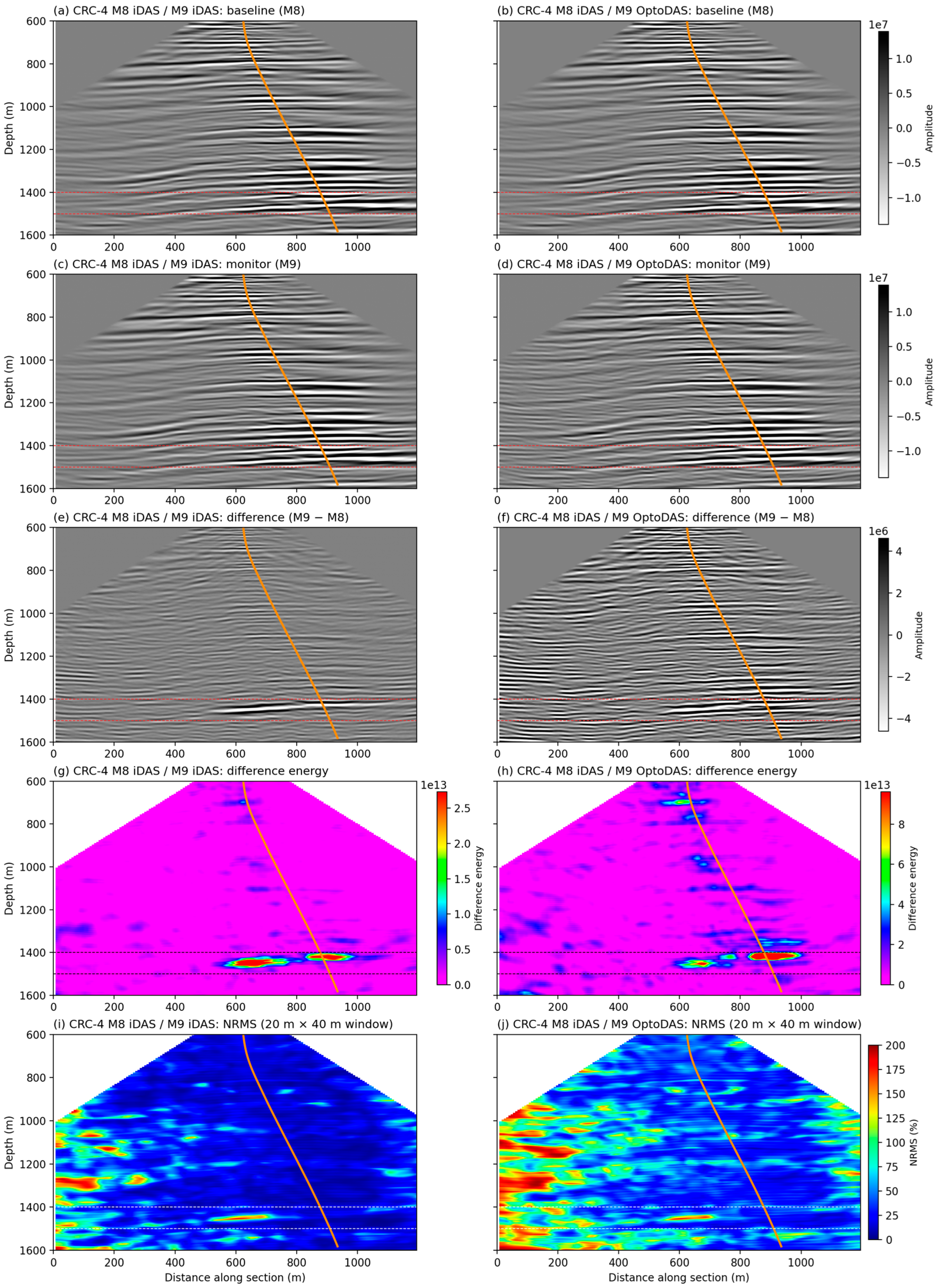
Figure 13. Plan-view maps of maximum RMS difference and NRMS attributes at the reservoir level extracted from migrated 3D DAS-VSP volumes for three acquisition configurations. Panels (a,b): CRC-4 same-configuration (M8/M9 iDAS). Panels (c,d): CRC-4 cross-configuration (M8 iDAS/M9 OptoDAS). Panels (e,f): CRC-3 cross-configuration (M8 iDAS/M9 OptoDAS). Left column (a,c,e): maximum RMS difference within the injection interval (1400–1500 m depth), each shown on its own colour scale; the comparison between cases is quantified in Table 2. Right column (b,d,f): NRMS at 1350 m using a 10 m vertical window.

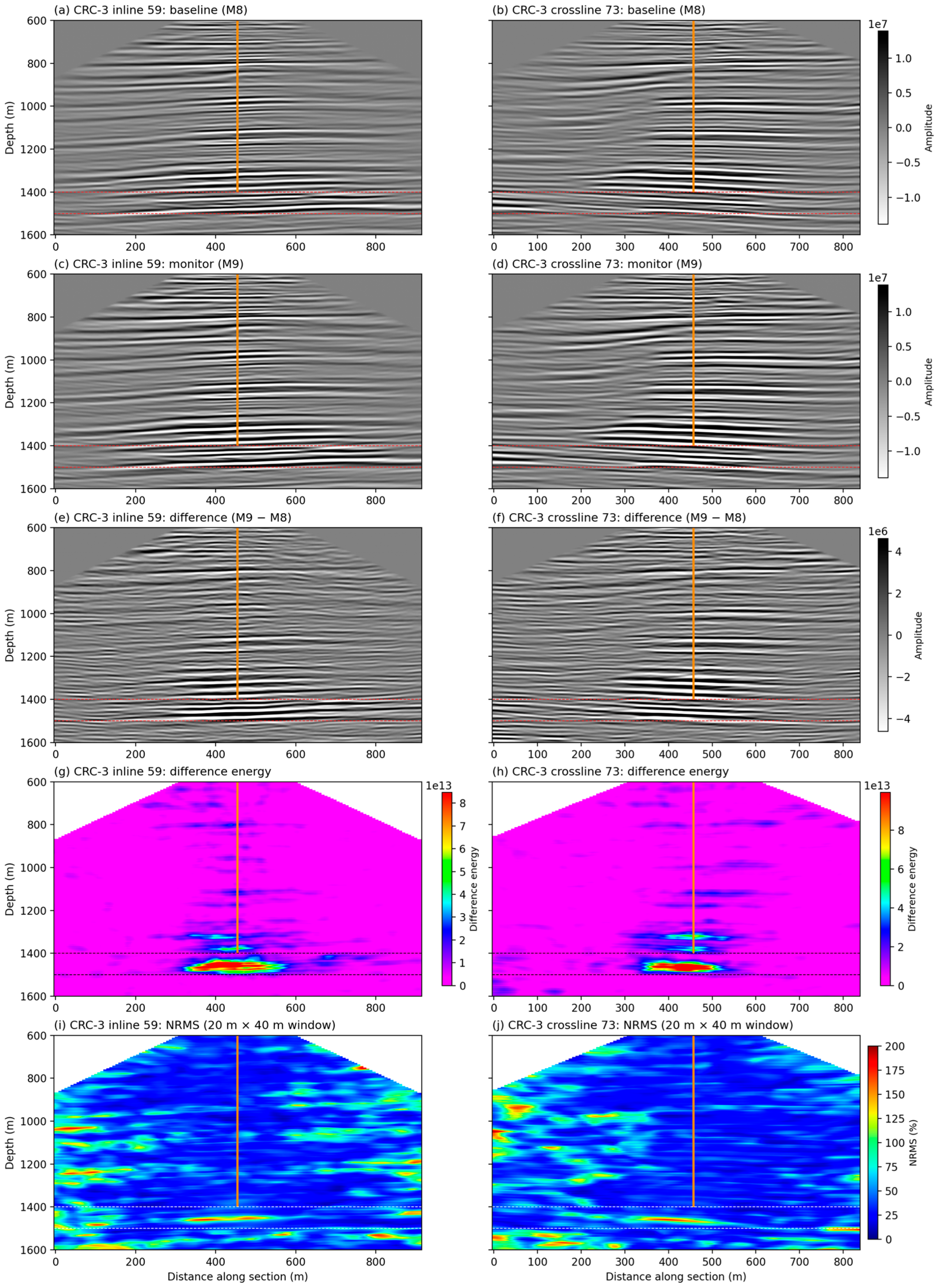
Figure 13. Plan-view maps of maximum RMS difference and NRMS attributes at the reservoir level extracted from migrated 3D DAS-VSP volumes for three acquisition configurations. Panels (a,b): CRC-4 same-configuration (M8/M9 iDAS). Panels (c,d): CRC-4 cross-configuration (M8 iDAS/M9 OptoDAS). Panels (e,f): CRC-3 cross-configuration (M8 iDAS/M9 OptoDAS). Left column (a,c,e): maximum RMS difference within the injection interval (1400–1500 m depth), each shown on its own colour scale; the comparison between cases is quantified in Table 2. Right column (b,d,f): NRMS at 1350 m using a 10 m vertical window.

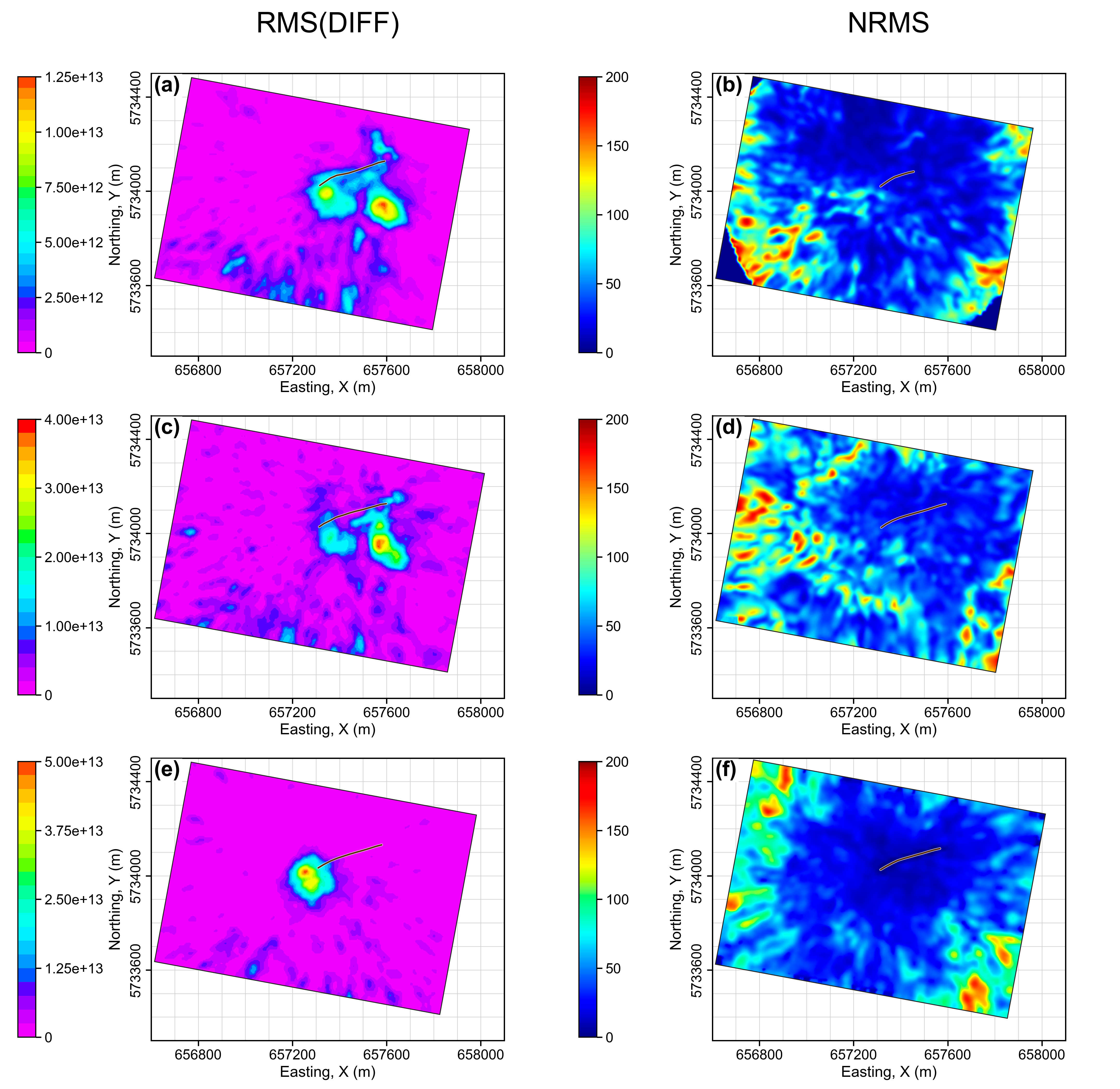
Table 2. Time-lapse RMS amplitudes and anomaly-to-background contrast at CRC-4 and CRC-3, computed from the migrated volumes. Anomaly RMS is measured over the reservoir interval (1400–1500 m) within the anomaly area, and background RMS over the control interval (1200–1300 m) within the same area. Near-maximum is the 99th percentile. Contrast is anomaly RMS divided by background RMS; brackets give 95% block-bootstrap confidence intervals.

Case	Anomaly RMS, Near-Maximum	Anomaly RMS, Mean	Background RMS	Peak Contrast [95% CI]	Mean Contrast [95% CI]
CRC-4 same	4.06 × 106	2.30 × 106	0.81 × 106	5.0 [4.1–5.5]	2.8 [2.5–3.2]
CRC-4 cross	7.39 × 106	4.28 × 106	2.14 × 106	3.5 [3.1–3.7]	2.0 [1.8–2.2]
CRC-3 cross	7.95 × 106	5.36 × 106	2.15 × 106	3.7 [3.5–3.9]	2.5 [2.3–2.7]

Table 2. Time-lapse RMS amplitudes and anomaly-to-background contrast at CRC-4 and CRC-3, computed from the migrated volumes. Anomaly RMS is measured over the reservoir interval (1400–1500 m) within the anomaly area, and background RMS over the control interval (1200–1300 m) within the same area. Near-maximum is the 99th percentile. Contrast is anomaly RMS divided by background RMS; brackets give 95% block-bootstrap confidence intervals.

Case	Anomaly RMS, Near-Maximum	Anomaly RMS, Mean	Background RMS	Peak Contrast [95% CI]	Mean Contrast [95% CI]
CRC-4 same	4.06 × 106	2.30 × 106	0.81 × 106	5.0 [4.1–5.5]	2.8 [2.5–3.2]
CRC-4 cross	7.39 × 106	4.28 × 106	2.14 × 106	3.5 [3.1–3.7]	2.0 [1.8–2.2]
CRC-3 cross	7.95 × 106	5.36 × 106	2.15 × 106	3.7 [3.5–3.9]	2.5 [2.3–2.7]

At CRC-4, the M8 and M9 migrated volumes show closely aligned reflector geometries in both the same- and cross-configuration comparisons (Figure 11a–d). In the same-configuration case, the difference volume contains a spatially focused anomaly near the reservoir interval, with comparatively low residual energy in the surrounding area (Figure 11e). The corresponding difference-energy section shows an anomaly-to-background contrast of 5.0:1 (Figure 11g; Table 2). In the cross-configuration comparison, an anomaly occurs at a similar depth and spatial position (Figure 11f), with a contrast of 3.5:1 (Figure 11h; Table 2). The cross-configuration difference section (Figure 11f) also exhibits greater spatial variability outside the principal anomaly, reducing its separation from the surrounding background.

The NRMS sections in Figure 11i,j provide a complementary measure of image-domain repeatability. Considering only the interval above 1400 m, the same-configuration comparison is characterised predominantly by lower NRMS values through the central part of the image, particularly around the well. The cross-configuration section contains higher and more spatially variable NRMS over the same depth range, including broader zones of elevated NRMS away from the well.

Figure 12 shows the corresponding cross-configuration result at CRC-3. The migrated baseline and monitor volumes remain kinematically aligned in both the inline and crossline sections (Figure 12a–d). The time-lapse difference sections contain a compact and spatially localised anomaly near the reservoir interval (Figure 12e,f). Because the M9 OptoDAS fibre terminated just above the reservoir interval, this anomaly is imaged by upgoing reflections recorded at receivers above it. Only receiver depths common to both surveys were used, so the baseline image is formed from the same receivers; receivers extending into the reservoir would add at most about 5% fold, and only within about 50 m of the well. The corresponding difference-energy sections show an anomaly-to-background contrast of 3.7:1 (Table 2), with comparatively little surrounding energy around the principal response (Figure 12g,h). The reservoir anomaly is therefore clearly separated from the local background.

Above 1400 m, the NRMS sections (Figure 12i,j) are comparatively low around the well and become higher and more spatially variable toward the ends of the sections. The CRC-3 result therefore combines a clearly localised reservoir response with a relatively low local non-repeatability background around the well. However, because no same-configuration M9 reference is available at CRC-3, the origin of this lower background cannot be separated into configuration-dependent and local acquisition or imaging effects.

Figure 13 compares the plan-view reservoir RMS response with the corresponding above-reservoir NRMS background for each case. NRMS is calculated using a 10 m vertical window centred at a depth of 1350 m, above the reservoir interval where no injection-related change is expected.

For the CRC-4 same-configuration comparison, the reservoir RMS map (Figure 13a) shows a spatially concentrated anomaly near the well, with an anomaly-to-background contrast of 5.0:1 (Table 2) and relatively limited surrounding RMS energy. The corresponding NRMS map (Figure 13b) shows comparatively low values around the well, mostly below approximately 50%, with higher NRMS concentrated farther from the well and toward the image margins. The localised reservoir response is therefore associated with a comparatively low non-repeatability background in the central part of the image.

The CRC-4 cross-configuration RMS map (Figure 13c) contains an anomaly at a similar spatial position, but its anomaly-to-background contrast is lower, 3.5:1 (Table 2), and the surrounding RMS response is more spatially variable. The corresponding NRMS map (Figure 13d) shows higher and more spatially heterogeneous values than the same-configuration case, with much of the central portion of the image predominantly within the 40–90% range and local areas exceeding 90%. Elevated NRMS also extends closer to the well than in the same-configuration result. The CRC-4 cross-configuration case, therefore, combines reduced separation of the reservoir RMS anomaly from the surrounding background with a higher and more spatially variable non-repeatability background. Both CRC-4 NRMS maps nevertheless show increasing values toward the outer parts of the image, indicating that this outward deterioration in repeatability is not unique to the combined configuration change; it is consistent with the decrease in illumination and migration fold with distance from the well.

At CRC-3, the reservoir RMS map (Figure 13e) shows a compact anomaly centred close to the well, with an anomaly-to-background contrast of 3.7:1 (Table 2) and little surrounding RMS energy. The corresponding NRMS map (Figure 13f) shows comparatively low values around the well, mostly below approximately 50%, while higher values are concentrated farther from the well and toward the margins of the migrated image. The CRC-3 result, therefore, combines a strongly localised reservoir response with a comparatively low local non-repeatability background. Because no same-configuration M9 reference is available at CRC-3, however, the comparatively low central NRMS cannot be attributed specifically to the sensing configuration or separated from local acquisition and imaging effects.

Table 2 quantifies the reservoir response at both wells. For each case, the RMS amplitude of the time-lapse difference was computed in the reservoir interval (1400–1500 m) and in a control interval above the reservoir (1200–1300 m), where no injection-related change is expected. The anomaly area is the region around each well where the reservoir RMS exceeds 30% of the anomaly peak (about 0.1 km² at CRC-4 and 0.05 km² at CRC-3); at CRC-4 the same area is used for both cases. The contrast is the anomaly RMS divided by the control-interval RMS over the same area, with 95% confidence intervals from a non-overlapping spatial block bootstrap [28] (2000 resamples, 60 m blocks). The anomaly is considered distinguishable from the non-repeatability background when the lower 95% confidence bound of its contrast exceeds 1; this holds for all three cases. At CRC-4 the intervals for the two cases do not overlap, so the reduction in contrast is significant. The cross-configuration reservoir RMS is not lower, at about 1.8 times the same-configuration value, but its background is about 2.6 times higher. The lower contrast is therefore associated with the higher non-repeatability background rather than a loss of reservoir amplitude; because the reservoir RMS also includes this background, its higher value does not indicate a stronger CO₂ response. At CRC-3 the anomaly is also distinguishable (3.7:1); as no same-configuration reference is available there, this contrast is not used to assess the effect of the configuration change.

To compare the position of the recovered anomaly, an anomaly map was formed for each CRC-4 configuration from the maximum RMS amplitude of the time-lapse difference (22 m running window) within the reservoir interval. This was done both with each configuration migrated using its own source set and with both migrated using an identical source set. In both cases, the two maps align best with no lateral shift larger than one grid cell (7.5 m) (correlation 0.78 and 0.84, respectively), and the depth of the maximum response agrees within one depth sample (2 m) in both the western and eastern parts of the anomaly. Applying the anomaly-area definition of Table 2 to each configuration separately gives anomaly areas of 0.081 and 0.085 km², of which about 75% coincide; the main difference is a weaker western part of the anomaly near the well in the cross-configuration result. The two M9 monitor images correlate at 0.97–0.98 over the reservoir interval, with a median relative depth shift of 0.8 and 0.7 m, respectively, below the depth sampling, so the configuration change introduces no measurable traveltime shift. The CO₂ response is therefore recovered at the same lateral position and depth, and with a similar extent, in both configurations, although its western part is weaker. An analytical sensitivity estimate was also made. The background non-repeatability was characterised by the mean and 99th percentile of the RMS time-lapse difference in the control interval, and the latter was used as the detection threshold. Assuming uncorrelated signal and background, the threshold is reached when the CO₂-related signal equals the square root of the difference between the squared 99th-percentile and mean background RMS. Relative to the same-configuration CO₂-related signal, this threshold is 0.28 (95% CI 0.20–0.39) under the same-configuration background and 0.67 (0.60–0.80) under the cross-configuration background. These values are specific to this case and assume that the control-interval background is representative of the background at reservoir depth.

Taken together, the migrated results show that the principal reservoir-scale time-lapse response remains spatially localised and distinguishable in both cross-configuration comparisons. At CRC-4, the cross-configuration result shows a higher and more spatially variable non-repeatability background than the same-configuration reference, together with a lower reservoir RMS anomaly-to-background contrast (3.5:1 compared with 5.0:1; Table 2). The anomaly is nevertheless recovered at the same lateral position and depth in both configurations. At CRC-3, the principal anomaly remains compact and well separated from the surrounding RMS background (3.7:1), while the above-reservoir NRMS remains comparatively low around the well.

5. Discussion

5.1. Configuration-Dependent Repeatability in the Gather Domain

The established Otway Stage 3 workflow [18] was retained, with adaptations only where needed to place the datasets on a comparable basis. The main asymmetry is the PCA noise attenuation, applied only to the noisier OptoDAS data. As a control, the same PCA was applied to the M8 and M9 iDAS data for 200 CRC-4 shots at source offsets up to 800 m. Its effect was negligible: 74–86% of the shots were left unchanged, the modified shots correlated with their input at 1.000 and their first-arrival SNR changed by less than 1 dB, and the median M8 iDAS–M9 iDAS NRMS (42.1%) and correlation (0.884) were unchanged. The PCA therefore introduces no artefact through the iDAS data for these shots, although a minor contribution from the OptoDAS attenuation itself cannot be excluded.

First-arrival NRMS is used to quantify acquisition and sensing-system repeatability in the shot gather domain. The direct P-wave provides a strong and consistently sampled reference for comparing cross-vintage and cross-configuration data. This measure does not directly quantify repeatability of the reservoir response, whose significance is assessed from the final migrated volumes. It is therefore used here as a shot-level quality-control measure, whereas image-domain NRMS and the anomaly-to-background contrast are used to assess repeatability at the reservoir.

At CRC-4, both fibres were recorded during the same M9 acquisition, so the M9 iDAS–M9 OptoDAS comparison provides a direct constraint on cross-configuration mismatch without the M8–M9 survey interval. After processing, the NRMS calculated around the first arrival remains higher than the same-configuration baseline–monitor result and close to the M8 iDAS–M9 OptoDAS value. This indicates that a substantial mismatch associated with the combined configuration change remains under same-vintage acquisition conditions.

The stage-by-stage response shows how the measured mismatch changes following each correction. PCA-based noise attenuation was applied only to the OptoDAS data, motivated by their 11.35 dB lower first-arrival SNR and the coherent, low-rank character of the residual noise. The accompanying increases in OptoDAS SNR and waveform correlation, together with the reduction in NRMS, support the elevated noise level as an important contributor to the mismatch associated with the combined configuration change. The OptoDAS SNR nevertheless remains 8.61 dB below the iDAS reference after denoising, indicating that the noise difference is only partly reduced by the present workflow and that its contribution cannot be isolated quantitatively from the remaining mismatch.

Deterministic deconvolution and shot-wise Wiener matching produce a combined median NRMS reduction of 30.0 percentage points for the CRC-4 same-configuration M8–M9 comparison and 33.1 percentage points for the cross-configuration M8–M9 comparison, compared with only 6.4 percentage points for the same-vintage M9 iDAS–OptoDAS comparison. This pattern is consistent with a greater contribution from survey-dependent waveform differences in the baseline–monitor comparisons. After the full processing sequence, the median first-arrival NRMS is 10.8% for the same-configuration comparison, 20.3% for the same-vintage M9 iDAS–M9 OptoDAS comparison and 22.1% for the cross-vintage cross-configuration comparison. Because the same-vintage value, which involves no survey interval, is close to the cross-configuration value and about twice the same-configuration value, most of the cross-configuration mismatch is associated with the configuration change rather than with the time between surveys. The significance of this residual mismatch for time-lapse monitoring is therefore evaluated from the final migrated volumes.

5.2. Image-Domain Repeatability and Preservation of the 4D Response

The migrated-volume analysis provides the principal test of whether the reservoir-scale time-lapse response remains distinguishable from the non-repeatability background in the cross-configuration data. At CRC-4, comparison with the same-configuration reference shows that the residual effect of the combined configuration change is expressed mainly as increased background variability and reduced anomaly-to-background separation. The reservoir RMS contrast decreases from 5.0:1 (95% CI 4.1–5.5) in the same-configuration case to 3.5:1 (95% CI 3.1–3.7) in the cross-configuration case (Table 2), while the principal anomaly remains spatially preserved. This indicates that the processing workflow retains the main 4D response, although with a reduced margin of separation from the surrounding background.

The above-reservoir NRMS control, calculated at 1350 m over a 10 m vertical window, provides an independent check on whether spatially elevated residual energy should be interpreted as reservoir response or as non-repeatability. At CRC-4, the increase in NRMS toward the left side occurs in both the same- and cross-configuration cases. Its persistence under unchanged sensing configuration, together with the rightward deviation of CRC-4, supports an acquisition- and imaging-related contribution to this spatial trend rather than a configuration-specific or reservoir-related origin.

At CRC-3, the reservoir anomaly is distinguishable from the background (3.7:1; Table 2), and the above-reservoir NRMS is comparatively low around the well. Because no same-configuration reference is available at CRC-3, the cause of this result cannot be isolated; it shows that the anomaly is also recovered at a second well, but it is not used to assess the configuration change. As in Stage 3 [18], differences between the images from the two wells may also reflect the 1D isotropic velocity model, which does not account for the anisotropy known at the site; because the same model was used within each well for the baseline and monitor datasets and for both configurations, it mainly affects the absolute image position rather than the baseline–monitor differences and the comparison between configurations.

5.3. Limitations and Conditions

This Otway field case provides a proof-of-concept for long-term DAS-VSP monitoring when sensing configurations change. Under the favourable acquisition and signal conditions examined here, useful time-lapse interpretation remained possible where acquisition repeatability was high and the principal reservoir response remained distinguishable from the residual mismatch.

The CRC-4 results also show that the adapted processing workflow reduces, but does not eliminate, the mismatch associated with the combined configuration change. Even after processing, the same-vintage iDAS–OptoDAS comparison retains appreciable mismatch, and the cross-configuration baseline–monitor result remains less repeatable than the same-configuration reference. This highlights the value of same-vintage overlap acquisition when a sensing configuration is changed, as it provides a direct measure of the difference between the existing and replacement configurations under shared acquisition conditions.

Several limitations constrain the generality of the results. Interrogator type, fibre type, and optical path changed simultaneously between the iDAS and OptoDAS configurations, and no auxiliary recordings are available to separate them. Their individual contributions therefore cannot be isolated, and the results describe the effect of the combined configuration change rather than that of any single component. Disentangling these effects would require controlled tests that vary one component at a time, for example, recording the same fibre with both interrogators, or both fibre types with the same interrogator. More importantly for practical detectability, the present field case benefits from repeatable source geometry, adequate signal quality and illumination, and a strong, spatially coherent time-lapse response. Weaker, more localised, or lower-amplitude changes under less favourable acquisition or illumination conditions may therefore be more difficult to distinguish from the residual non-repeatability background. Because these findings are drawn from a single site and a single baseline–monitor pair, their transfer to other sites, sensing configurations or survey intervals would need to be confirmed by further field cases.

For future long-term monitoring, maintaining consistent acquisition and sensing parameters remains preferable whenever possible. Where a configuration change is unavoidable, overlap acquisition between the existing and replacement systems during the same survey provides a direct means of characterising the additional mismatch before the new configuration is used for subsequent time-lapse interpretation.

Such overlap can be acquired without additional shots when both systems record the same survey; the main added costs are the second interrogator, its fibre, and the recording and processing of the additional data, while the source effort is shared rather than repeated. The paired recordings can provide a direct measure of the difference between the configurations, including interrogator settings such as gauge length, and can be used to derive matching parameters such as channel-depth registration, amplitude scaling and waveform matching. The second system may also provide redundancy if a fibre or interrogator fails, as is the case at CRC-3 in the present study. Because this difference can vary among shots, with distance from the well, and between wells with different geometry, optical path length and fibre, a limited number of shared shots may not adequately assess its effect on the final image, and including each monitored well may be beneficial. The comparison may use the first-arrival signal-to-noise ratio and NRMS and, where baseline and monitor images are available, the anomaly-to-background contrast.

6. Conclusions

This proof-of-concept field case demonstrates that the principal CO₂-related DAS-VSP time-lapse response remained distinguishable in the Otway M8–M9 comparisons under the favourable field conditions examined. The main reservoir-scale anomaly was recovered in both CRC-4 and CRC-3 despite the additional non-repeatability introduced by the combined configuration change.

The combined configuration change nevertheless imposed a clear repeatability penalty, which cannot be attributed to any one of its components. Residual mismatch remained after processing, and at CRC-4 the cross-configuration image showed a higher non-repeatability background and reduced anomaly-to-background contrast relative to the same-configuration reference. At CRC-4, the configuration change increased the median first-arrival NRMS of the shot gathers from 10.8% to 22.1% and reduced the anomaly-to-background contrast of the migrated images from 5.0:1 to 3.5:1. The present workflow therefore mitigates, but does not fully remove, the additional mismatch associated with the configuration change.

These results were obtained under favourable field conditions, including repeatable acquisition, adequate signal quality and illumination, and a sufficiently strong and spatially coherent reservoir response. In this CRC-4 case, a CO₂-related signal of about two-thirds of the observed same-configuration amplitude would reach the selected detection threshold under the cross-configuration background, compared with about one-quarter under the same-configuration background. Under less favourable conditions or for weaker anomalies, the reduced separation from the non-repeatability background may therefore become more limiting. For long-term monitoring, maintaining a consistent sensing configuration remains preferable; where changes are unavoidable, overlapping acquisition between existing and replacement systems provides a practical means of assessing configuration-associated mismatch.

References

- Jenkins, C.R.; Cook, P.J.; Ennis-King, J.; Undershultz, J.; Boreham, C.; Dance, T.; de Caritat, P.; Etheridge, D.M.; Freifeld, B.M.; Hortle, A.; et al. Safe storage and effective monitoring of CO2 in depleted gas fields. Proc. Natl. Acad. Sci. USA 2012, 109, E35–E41. [Google Scholar] [CrossRef] [Scilit] [PubMed]
- Oldenburg, C.M. Are we all in concordance with the meaning of the word conformance, and is our definition in conformity with standard definitions? Greenh. Gases Sci. Technol. 2018, 8, 210–214. [Google Scholar] [CrossRef] [Scilit]
- Arts, R.; Eiken, O.; Chadwick, A.; Zweigel, P.; van der Meer, B.; Zinszner, B. Monitoring of CO2 injected at Sleipner using time-lapse seismic data. Energy 2004, 29, 1383–1392. [Google Scholar] [CrossRef] [Scilit]
- Dean, K.; Tucker, O. A risk-based framework for Measurement, Monitoring and Verification (MMV) of the Goldeneye storage complex for the Peterhead CCS project, UK. Int. J. Greenh. Gas Control 2017, 61, 1–15. [Google Scholar] [CrossRef] [Scilit]
- White, D.J.; Roach, L.A.N.; Roberts, B. Time-lapse seismic performance of a sparse permanent array: Experience from the Aquistore CO2 storage site. Geophysics 2015, 80, WA35–WA48. [Google Scholar] [CrossRef] [Scilit]
- Lüth, S.; Bergmann, P.; Huang, F.; Ivandic, M.; Ivanova, A.; Juhlin, C.; Kempka, T. 4D seismic monitoring of CO2 storage during injection and post-closure at the Ketzin pilot site. Energy Procedia 2017, 114, 5761–5767. [Google Scholar] [CrossRef] [Scilit]
- Pevzner, R.; Urosevic, M.; Popik, D.; Shulakova, V.; Tertyshnikov, K.; Caspari, E.; Correa, J.; Dance, T.; Kepic, A.; Glubokovskikh, S.; et al. 4D surface seismic tracks small supercritical CO2 injection into the subsurface: CO2CRC Otway Project. Int. J. Greenh. Gas Control 2017, 63, 150–157. [Google Scholar] [CrossRef] [Scilit]
- Roach, L.A.N.; White, D.J. Evolution of a deep CO2 plume from time-lapse seismic imaging at the Aquistore storage site, Saskatchewan, Canada. Int. J. Greenh. Gas Control 2018, 74, 79–86. [Google Scholar] [CrossRef] [Scilit]
- Ivandic, M.; Juhlin, C.; Lüth, S.; Bergmann, P.; Kashubin, A.; Sopher, D.; Ivanova, A.; Baumann, G.; Henninges, J. Geophysical monitoring at the Ketzin pilot site for CO2 storage: New insights into the plume evolution. Int. J. Greenh. Gas Control 2015, 32, 90–105. [Google Scholar] [CrossRef] [Scilit]
- Mathieson, A.; Midgley, J.; Wright, I.; Saoula, N.; Ringrose, P. In Salah CO2 storage JIP: CO2 sequestration monitoring and verification technologies applied at Krechba, Algeria. Energy Procedia 2011, 4, 3596–3603. [Google Scholar] [CrossRef] [Scilit]
- Ringrose, P.S.; Mathieson, A.S.; Wright, I.W.; Selama, F.; Hansen, O.; Bissell, R.; Saoula, N.; Midgley, J. The In Salah CO2 storage project: Lessons learned and knowledge transfer. Energy Procedia 2013, 37, 6226–6236. [Google Scholar] [CrossRef] [Scilit]
- Ahmadi, A.B.; Morozov, I. Time-lapse VSP data analysis from Weyburn CO2 Project. In Proceedings of the CSPG CSEG CWLS Convention, Calgary, AB, Canada, 9–13 May 2011. [Google Scholar]
- Couëslan, M.L.; Ali, S.; Campbell, A.; Nutt, W.L.; Leaney, W.S.; Finley, R.J. Monitoring CO2 injection for carbon capture and storage using time-lapse 3D VSPs. Lead. Edge 2013, 32, 1268–1276. [Google Scholar] [CrossRef] [Scilit]
- Daley, T.M.; Freifeld, B.M.; Ajo-Franklin, J.; Dou, S.; Pevzner, R.; Shulakova, V.; Kashikar, S.; Miller, D.E.; Goetz, J.; Henninges, J.; et al. Field testing of fiber-optic distributed acoustic sensing (DAS) for subsurface seismic monitoring. Lead. Edge 2013, 32, 699–706. [Google Scholar] [CrossRef] [Scilit]
- Mateeva, A.; Lopez, J.; Potters, H.; Mestayer, J.; Cox, B.; Kiyashchenko, D.; Wills, P.; Grandi, S.; Hornman, K.; Kuvshinov, B.; et al. Distributed acoustic sensing for reservoir monitoring with vertical seismic profiling. Geophys. Prospect. 2014, 62, 679–692. [Google Scholar] [CrossRef] [Scilit]
- Pevzner, R.; Gurevich, B.; Pirogova, A.; Tertyshnikov, K.; Glubokovskikh, S. Repeat well logging using earthquake wave amplitudes measured by distributed acoustic sensors. Lead. Edge 2020, 39, 513–517. [Google Scholar] [CrossRef] [Scilit]
- Correa, J.; Pevzner, R.; Bona, A.; Tertyshnikov, K.; Freifeld, B.; Robertson, M.; Daley, T. 3D vertical seismic profile acquired with distributed acoustic sensing on tubing installation: A case study from the CO2CRC Otway Project. Interpretation 2019, 7, SA11–SA19. [Google Scholar] [CrossRef] [Scilit]
- Yurikov, A.; Tertyshnikov, K.; Yavuz, S.; Shashkin, P.; Isaenkov, R.; Sidenko, E.; Glubokovskikh, S.; Barraclough, P.; Pevzner, R. Seismic monitoring of CO2 geosequestration using multi-well 4D DAS VSP: Stage 3 of the CO2CRC Otway project. Int. J. Greenh. Gas Control 2022, 119, 103726. [Google Scholar] [CrossRef] [Scilit]
- Bellefleur, G.; Schetselaar, E.; Wade, D.; White, D.; Enkin, R.; Schmitt, D.R. Vertical seismic profiling using distributed acoustic sensing with scatter-enhanced fibre-optic cable at the Cu–Au New Afton porphyry deposit, British Columbia, Canada. Geophys. Prospect. 2020, 68, 313–333. [Google Scholar] [CrossRef] [Scilit]
- Yurikov, A.; Tertyshnikov, K.; Isaenkov, R.; Sidenko, E.; Yavuz, S.; Glubokovskikh, S.; Barraclough, P.; Shashkin, P.; Pevzner, R. Multiwell 3D distributed acoustic sensing vertical seismic profile imaging with engineered fibers: CO2CRC Otway Project case study. Geophysics 2021, 86, D241–D248. [Google Scholar] [CrossRef] [Scilit]
- Pevzner, R.; Glubokovskikh, S.; Isaenkov, R.; Shashkin, P.; Tertyshnikov, K.; Yavuz, S.; Gurevich, B.; Correa, J.; Wood, T.; Freifeld, B. Monitoring subsurface changes by tracking direct-wave amplitudes and traveltimes in continuous DAS VSP data. Geophysics 2022, 87, A1–A6. [Google Scholar] [CrossRef] [Scilit]
- Almukhametova, A.; Tertyshnikov, K.; Beloborodov, N.; Collet, O.; Gurevich, B.; Isaenkov, R.; Al Marzooq, M.; Shashkin, P.; Vorobev, M.; Pevzner, R. Processing four-dimensional vertical seismic profiling in the CO2CRC Otway Stage 4 Project. J. Seism. Explor. 2026, 35, 026040015. [Google Scholar] [CrossRef] [Scilit]
- Miya, T.; Terunuma, Y.; Hosaka, T.; Miyashita, T. Ultimate low-loss single-mode fibre at 1.55 μm. Electron. Lett. 1979, 15, 106–108. [Google Scholar] [CrossRef] [Scilit]
- Dean, T.; Cuny, T.; Hartog, A.H. The effect of gauge length on axially incident P-waves measured using fibre optic distributed vibration sensing. Geophys. Prospect. 2017, 65, 184–193. [Google Scholar] [CrossRef] [Scilit]
- Kragh, E.; Christie, P. Seismic repeatability, normalized rms, and predictability. Lead. Edge 2002, 21, 640–647. [Google Scholar] [CrossRef] [Scilit]
- Pevzner, R.; Isaenkov, R.; Yavuz, S.; Yurikov, A.; Tertyshnikov, K.; Shashkin, P.; Gurevich, B.; Correa, J.; Glubokovskikh, S.; Wood, T.; et al. Seismic monitoring of a small CO2 injection using a multi-well DAS array: Operations and initial results of Stage 3 of the CO2CRC Otway project. Int. J. Greenh. Gas Control 2021, 110, 103437. [Google Scholar] [CrossRef] [Scilit]
- Bona, A.; Dean, T.; Correa, J.; Pevzner, R.; Tertyshnikov, K.V.; van Zaanen, L. Amplitude and phase response of DAS receivers. In Proceedings of the 79th EAGE Conference and Exhibition 2017, Paris, France, 12–15 June 2017; pp. 1–5. [Google Scholar] [CrossRef] [Scilit]
- Lahiri, S.N. Uncertainty quantification in robust inference for irregularly spaced spatial data using block bootstrap. Sankhya A 2018, 80, 173–221. [Google Scholar] [CrossRef] [Scilit]
Disclaimer/Publisher’s Note: The statements, opinions and data contained in all publications are solely those of the individual author(s) and contributor(s) and not of MDPI and/or the editor(s). MDPI and/or the editor(s) disclaim responsibility for any injury to people or property resulting from any ideas, methods, instructions or products referred to in the content. |
© 2026 by the authors. Licensee MDPI, Basel, Switzerland. This article is an open access article distributed under the terms and conditions of the Creative Commons Attribution (CC BY) license.