Forest Digital Terrain Model from Copernicus GLO-30 DEM and GEDI L2A Using an Explainable Boosting Machine

Highlights

What are the main findings?

•

The CopDEM–GEDI elevation offset was estimated with an Explainable Boosting Machine (EBM) to generate a continuous forest DTM, with RMSEs of 4.10 and 3.67 m against independent airborne LiDAR.

•

The CopDEM height error mask (HEM), canopy cover, and aspect contributed most to the estimated offset, while the magnitude and direction of predictor contributions varied with canopy–terrain conditions and between regions.

What are the implications of the main findings?

•

Decomposing the estimated offset by predictor allows the correction to be interpreted in terms of canopy, terrain, and data-uncertainty information, not only by its final accuracy.

•

Linking predictor contributions with independent residuals identifies conditions under which forest DTMs derived from CopDEM and GEDI should be used with caution.

Abstract

Accurate ground elevation beneath forest canopies is important for terrain and forest-structure analysis, yet satellite-based elevation data can be affected by canopy and terrain conditions, while spaceborne light detection and ranging (LiDAR) provides ground elevations only at discrete locations. Here, the elevation offset between the Copernicus GLO-30 DEM (CopDEM) and Global Ecosystem Dynamics Investigation (GEDI) L2A ground elevation was estimated using an Explainable Boosting Machine (EBM) with topographic, canopy-structure, and CopDEM-uncertainty predictors to generate continuous forest digital terrain models (DTMs) for two regions in the Republic of Korea. Validation against independent airborne LiDAR data showed root mean square errors (RMSEs) of the proposed DTM of 4.10 m in the central-western region and 3.67 m in the eastern region. In the EBM, the CopDEM height error mask (HEM), canopy cover, and aspect contributed most to the estimated offset, and the magnitude and direction of their contributions varied across canopy–terrain conditions and between regions. Residual bias increased with canopy height and became more negative on steep slopes, where RMSE also increased. These results show that the proposed approach can generate continuous forest DTMs while quantifying the contributions of the main predictors to the offset, their variation across environmental conditions, and the conditions under which residual errors increase.

1. Introduction

A digital terrain model (DTM) represents the elevation of the bare-earth surface, excluding vegetation and artificial structures [1]. In forested areas, a DTM provides ground elevation information beneath the canopy and is essential for distinguishing terrain from vegetation effects and interpreting three-dimensional forest structure [2,3]. Because terrain relief and the vertical structure of vegetation occur together in forest environments, reliable ground elevation is needed to distinguish and interpret these two components.

Constructing accurate forest DTMs at regional to global scales remains challenging, and satellite-based elevation data have been widely used for this purpose. Interferometric synthetic aperture radar (InSAR) derives surface elevation from the phase difference between SAR observations acquired from different viewing positions [4]. Based on this technique, the TanDEM-X mission operated the two X-band SAR satellites TerraSAR-X and TanDEM-X as a single-pass interferometer to generate a consistent global elevation dataset [5]. However, over forests, the X-band signal is scattered within the canopy, so TanDEM-X elevations reflect vegetation structure rather than the ground [6,7]. The Copernicus GLO-30 Digital Elevation Model (CopDEM), derived from WorldDEM, generated from TanDEM-X observations and subsequently edited and refined, provides continuous global elevation information at approximately 30 m spacing and is publicly available, making it a useful base dataset for forest DTM generation [8,9].

Another active remote sensing technology, light detection and ranging (LiDAR), uses laser ranging to acquire three-dimensional information on forest canopies and the ground, from which vegetation structure and bare-earth elevation can be derived [10,11]. Airborne LiDAR provides dense three-dimensional measurements from which accurate forest DTMs can be generated and has therefore been widely used for terrain analysis and accuracy assessment. However, acquiring airborne LiDAR over large areas remains challenging because of the associated costs and operational constraints [12]. To observe forest vertical structure at the global scale, NASA developed the Global Ecosystem Dynamics Investigation (GEDI), a spaceborne full-waveform LiDAR instrument installed on the International Space Station (ISS) in December 2018 that began collecting science data in 2019 [13]. It characterizes forest structure from the ground to the upper canopy but provides spatially discrete point measurements along the ISS orbit, leaving unsampled gaps between them. Thus, CopDEM provides spatially continuous elevation information, whereas GEDI provides ground elevation at discrete locations; integrating the two enables sparse ground-elevation measurements to be extended into a continuous forest DTM.

Accordingly, various remote sensing datasets, including InSAR and LiDAR observations, have been used to estimate bare-earth terrain and construct DTMs. Yamazaki et al. [14] developed the global Multi-Error-Removed Improved-Terrain (MERIT) DEM using existing global DEMs, including Shuttle Radar Topography Mission (SRTM) and ALOS World 3D—30 m (AW3D30), together with Ice, Cloud, and land Elevation Satellite (ICESat) observations and vegetation-related data to reduce multiple elevation error components. Hawker et al. [15] applied Random Forest regression to predict the elevation difference between CopDEM and airborne LiDAR-based reference terrain elevations and used the predicted correction to produce the Forest And Buildings removed Copernicus DEM (FABDEM), a global DEM at approximately 30 m resolution with forest and building effects removed. Laipelt et al. [16] combined CopDEM, GEDI ground elevation, and Landsat- and Sentinel-derived multispectral data in a Gradient Tree Boost model to estimate and remove vegetation-related elevation bias and construct a digital terrain model for South America (ANADEM). More recently, Ho et al. [17] used GEDI and ICESat-2 ground-elevation points as training data and integrated CopDEM, AW3D30, and various ancillary datasets within a global-to-local Random Forest framework to construct the Global Ensemble Digital Terrain Model (GEDTM30), a global DTM at approximately 30 m resolution. Although these studies differ in the sensors and modeling approaches employed, they demonstrate that remote sensing datasets with different characteristics can be integrated with ground elevation information to generate spatially continuous bare-earth terrain elevation.

The accuracy of satellite-based elevation models has been assessed through independent validation against high-accuracy reference elevation data, mainly from airborne LiDAR. Gdulová et al. [18] evaluated the vertical accuracy of the TanDEM-X DEM in European mountains using airborne LiDAR-derived DTMs and DSMs and showed that the positive elevation offset relative to the reference terrain differed markedly between forested and non-forested areas, and that forest type, slope, and aspect affected accuracy. Uuemaa et al. [19] compared several global DEMs in four regions with different terrain and land cover conditions, using robust statistics such as the normalized median absolute deviation (NMAD) in addition to the root mean square error (RMSE) and mean error to account for non-normal error distributions, and identified slope as the factor with the strongest effect on accuracy. Meadows et al. [20] evaluated global DEMs, including CopDEM and FABDEM, against a large set of airborne LiDAR surveys and showed that land cover, particularly forest, was the main factor explaining vertical errors, whereas steep slopes were associated with wider error spreads. Elevation models have also been evaluated over surfaces modified by human activity. Aati and Avouac [21] compared a satellite-image-derived DEM with an airborne LiDAR DEM acquired at a different time over an open-pit mine, assessing accuracy over stable terrain and separating actual topographic change caused by mining. Okolie et al. [22] derived CopDEM elevation errors against airborne LiDAR in an urban area and corrected them by predicting the errors from terrain and land cover variables. These studies indicate that the accuracy of an elevation model is not fully described by overall statistics and must be evaluated according to terrain and surface conditions.

The elevation differences identified in such validations may be jointly related to several factors, including, in forested areas, the scattering and penetration of the signal within the canopy [6,7], terrain characteristics, and the uncertainty of the elevation data themselves [9]. In multi-source elevation estimation, information of different natures related to these factors is combined to form a single estimate. Consequently, even when estimates of similar magnitude are obtained, the magnitude and direction of the predictor contributions composing them may differ, and this composition may vary with canopy and terrain characteristics. Decomposing the final estimate into predictor contributions makes it possible to quantitatively distinguish the extent to which, and the direction in which, information related to canopy, terrain, and elevation uncertainty contributes to the estimate, and to interpret how the composition of the estimate changes under different canopy and terrain characteristics.

Such an analysis requires a model that represents the nonlinear relationships between the predictors and the estimated quantity while directly decomposing the final estimate into the contributions of individual predictors. For this purpose, an Explainable Boosting Machine (EBM) was applied in this study. The EBM is an intrinsically interpretable generalized additive model that learns each predictor–response relationship as a nonlinear shape function through boosting and constructs the final prediction as the additive sum of these predictor-specific terms [23,24,25]. The contribution of each predictor is therefore obtained directly as an individual model term without a separate post hoc interpretation step, allowing both its magnitude and direction to be analyzed. This structure allows the composition of the estimate to be analyzed quantitatively for each predictor while retaining nonlinear predictive relationships.

In this study, the difference between CopDEM and GEDI L2A ground elevation was defined as the elevation offset, which was estimated with an EBM and removed from CopDEM to generate a spatially continuous forest DTM. The study was conducted in two forested regions of the Republic of Korea with different terrain and canopy conditions. The specific objectives were as follows. First, the accuracy of the generated DTM was evaluated against airborne LiDAR DTMs that were not used in model training and compared with that of CopDEM and the globally trained products FABDEM and GEDTM30; this evaluation provides the basis on which the subsequent interpretation rests. Second, the contribution of predictor groups to the accuracy of the correction was assessed by refitting the model with subsets of predictors, and the magnitude and direction of the contributions of individual predictors to the elevation offset were quantified from the additive terms of the EBM, together with their variation with environmental conditions and between the two regions. Third, residual errors were analyzed by canopy height, slope, and forest type to identify the conditions under which the correction was insufficient or excessive and, therefore, under which the DTM should be used with caution. In addition, the sensitivity of the results to the GEDI filtering criteria and to forest loss between the acquisition periods of the datasets was examined.

2. Study Area and Data

2.1. Study Area

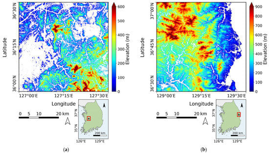
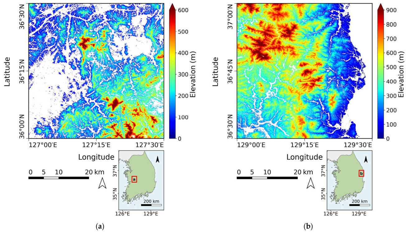
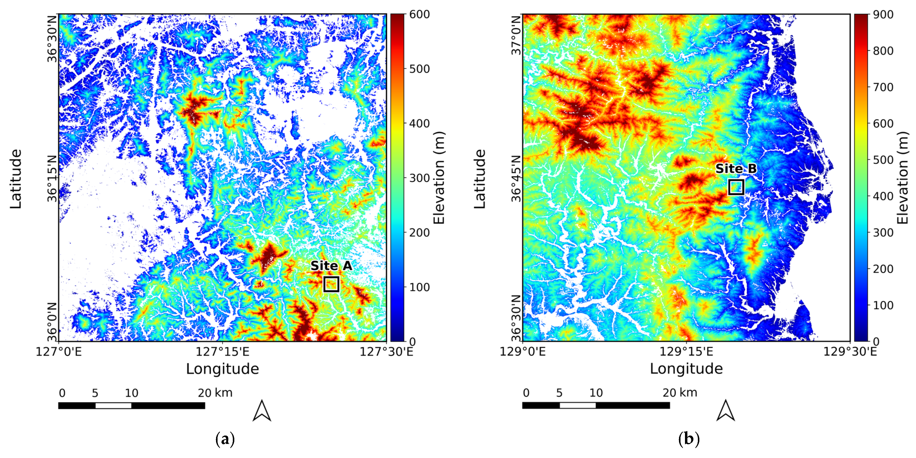
This study was conducted in two forested study regions located in the central-western and eastern parts of the Republic of Korea (Figure 1). Each region was defined as a 0.5° × 0.5° grid, within which the DTM was produced only over forested areas. The two regions differ in elevation, slope, and forest-type composition. Both regions were selected because high-resolution airborne LiDAR DTMs were available for independent evaluation; as this coverage spans only part of each grid, validation was restricted to forested areas within the LiDAR-covered extent.

Figure 1. CopDEM elevation maps of the two study regions: (a) the central-western region and (b) the eastern region. White areas indicate non-forest areas excluded from DTM production. The inset map in each panel shows the location of the corresponding study region (red box) in the Republic of Korea.

The central-western study region shown in Figure 1a is located within 127.0–127.5°E and 36.0–36.5°N. The DTM production area covers approximately 1273 km², where elevation ranges from 8 to 866 m (mean 225 m). The mean slope is approximately 20°, and terrain steeper than 25° accounts for about 26% of this area. Based on the national forest-type map of the Korea Forest Service [26], the forested area is dominated by broadleaf forest (55%), followed by coniferous (31%) and mixed forest (14%).

The eastern study region shown in Figure 1b is located within 129.0–129.5°E and 36.5–37.0°N. The DTM production area covers approximately 1820 km². Within the DTM production area, elevation ranges from 0 to 1211 m, with a mean of 428 m, higher than that of the central-western region. The mean slope is approximately 21°, comparable to that of the central-western region, whereas terrain with slopes greater than 25° accounts for a larger proportion of the DTM production area, approximately 34%. Based on the same forest-type map [26], coniferous forest is dominant, accounting for 49% of the forested area, while broadleaf forest accounts for 39% and mixed forest for 12%.

2.2. Data

2.2.1. CopDEM

CopDEM served two roles in this study: its difference from GEDI ground elevation defined the elevation offset, and the predicted offset was subsequently subtracted from CopDEM to generate the final DTM. The elevation observations underlying CopDEM were acquired by the TanDEM-X mission from 2011 to 2015 [5]. CopDEM is referenced horizontally to WGS84-G1150 (EPSG:4326) and vertically to Earth Gravitational Model 2008 (EGM2008; EPSG:3855), with a grid spacing of 1 arcsec [9]. According to the product specifications, the absolute vertical accuracy of CopDEM is <4 m at the 90% linear error level. Its relative vertical accuracy is <2 m for terrain with slopes ≤ 20% and <4 m for slopes > 20%, expressed as the 90% linear point-to-point error within a 1° × 1° area [9].

2.2.2. GEDI Ground Elevation

GEDI Level 2A (L2A) Elevation and Height Metrics data were used as ground-elevation observations for model training [13]. The GEDI data used in this study were Version 2 observations acquired from April 2019 to February 2025 and obtained through NASA Earthdata Search. Each GEDI point samples a surface area approximately 25 m in diameter, with consecutive points spaced about 60 m along-track and adjacent ground tracks separated by approximately 600 m across-track. The outermost of the eight ground tracks are separated by approximately 4.2 km across-track, and observations are acquired between approximately 51.6°N and 51.6°S [13]. Among the GEDI02_A parameters, elev_lowestmode, which represents the elevation of the center of the lowest selected waveform mode relative to the WGS84 reference ellipsoid, was used as the GEDI ground-elevation estimate [13].

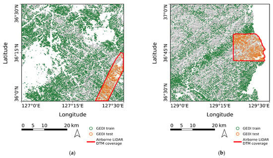
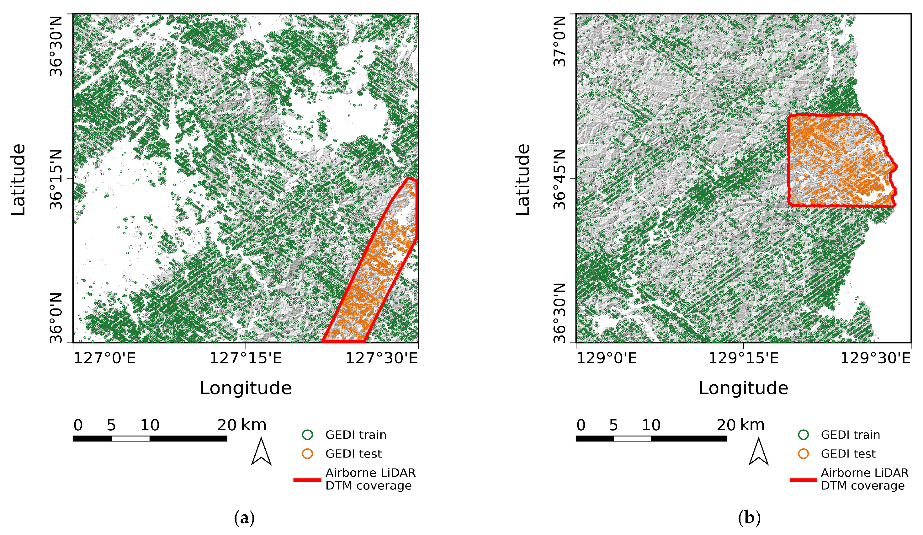
To ensure consistency in the vertical reference system, GEDI elevations referenced to the WGS84 ellipsoid were converted from ellipsoidal heights to orthometric heights referenced to EGM2008, matching the vertical reference system of CopDEM. The GEDI points were then filtered using quality flags and observation parameters, with the detailed filtering criteria described in Section 3.2. After filtering and aggregation to the CopDEM grid, 18,597 grid cells in the central-western region and 13,509 in the eastern region contained GEDI observations. Of these, the cells located outside the airborne LiDAR extent (17,668 in the central-western region and 12,118 in the eastern region) were used for model training, while cells within the LiDAR extent were excluded from training to maintain independent validation (Figure 2).

Figure 2. Spatial distribution of the filtered GEDI points in the two study regions. (a) Central-western region; (b) eastern region. Green points are used for training; orange points, falling inside the airborne LiDAR coverage (red outline), are excluded from training so that the validation area remains independent.

2.2.3. Predictors for Elevation Offset Estimation

The predictors used to estimate the elevation offset were grouped into three categories: topographic predictors, forest-related predictors, and a CopDEM uncertainty predictor (Table 1). The topographic predictors included CopDEM elevation, slope, aspect, roughness, hillshade, and geomorphon. Slope, aspect, roughness, and hillshade were obtained from OpenTopography as pre-computed products derived from CopDEM [27]. The geomorphon landform classification was derived from CopDEM using the geomorphon method [28] implemented in ArcGIS Pro (version 3.5.0; Esri, Redlands, CA, USA).

Table 1. Terrain and forest variables used to estimate the elevation offset.

Variable	Description	Source	Year	Ref.
Elevation	Digital elevation model	CopDEM GLO-30	2011–2015	[9]
Slope	Steepest gradient	CopDEM GLO-30 (OpenTopography)	2011–2015	[27]
Aspect	Slope orientation	CopDEM GLO-30 (OpenTopography)	2011–2015	[27]
Roughness	Local elevation variability	CopDEM GLO-30 (OpenTopography)	2011–2015	[27]
Hillshade	Modeled illumination	CopDEM GLO-30 (OpenTopography)	2011–2015	[27]
Geomorphon	Landform classification	CopDEM GLO-30	2011–2015	[28]
HEM	Per-pixel height uncertainty expressed as a standard deviation	CopDEM GLO-30	2011–2015	[9]
Canopy cover	Tree canopy cover fraction	GFCC Tree Cover	2015	[29]
Canopy height	Forest canopy height	GLAD Forest Canopy Height	2019	[30]
NDVI	Vegetation greenness index; (NIR − Red)/(NIR + Red)	Landsat-5 TM	2011	[31]
NDMI	Canopy moisture index; (NIR − SWIR1)/(NIR + SWIR1)	Landsat-5 TM	2011	[32]

The forest-related predictors included the 2015 tree canopy cover from the Global Forest Cover Change (GFCC) product [29], the 2019 global canopy height product of the Global Land Analysis and Discovery (GLAD) laboratory [30], and the Normalized Difference Vegetation Index (NDVI) [31] and Normalized Difference Moisture Index (NDMI) [32] derived from Landsat-5 Thematic Mapper (TM) imagery. The 2015 canopy cover epoch falls within the 2011–2015 TanDEM-X acquisition period underlying CopDEM. The 2019 canopy height product was selected because, among the available global canopy height products at approximately 30 m resolution, its epoch was the closest to the 2011–2015 TanDEM-X acquisition period. For NDVI and NDMI, Landsat-5 TM imagery acquired in 2011 was used to represent vegetation conditions within the TanDEM-X acquisition period while maintaining spectral consistency from a single sensor. Landsat-7 was excluded because imagery acquired after the failure of its Scan Line Corrector (SLC) in 2003 contains systematic data gaps [33]. Although Landsat-8 overlaps with the later part of the TanDEM-X acquisition period, data from different Landsat sensors were not combined because differences in their spectral response functions can introduce differences in reflectance and vegetation indices [34]. NDVI and NDMI were derived as median composites from multiple Landsat-5 TM scenes acquired in 2011.

The CopDEM uncertainty predictor was the Height Error Mask (HEM), which provides per-pixel height uncertainty expressed as a standard deviation derived from interferometric coherence and acquisition geometry [9]. The CopDEM GLO-30 grid defined the coordinate system, spatial extent, and grid spacing used throughout the analysis. The GFCC tree canopy cover, canopy height, NDVI, and NDMI have spatial resolutions of approximately 30 m but were not aligned with this grid and were therefore resampled to it using bilinear interpolation; nearest-neighbor resampling was used for geomorphon to preserve its categorical values.

2.2.4. Reference Data for Validation and Residual Analysis

Two 0.5 m airborne LiDAR DTMs, acquired at different times through the same airborne LiDAR survey program as the data reported in previous studies [35,36], were used as independent reference data for accuracy assessment of the proposed DTM. The central-western data were acquired on 3 April 2023 and the eastern data on 18 April 2019. Both airborne LiDAR datasets were horizontally referenced to EPSG:5187 and vertically referenced to EGM2008, consistent with the vertical reference system of CopDEM, so that no vertical datum transformation was required. For comparison with the proposed DTM and other elevation products, the airborne LiDAR DTMs were reprojected to EPSG:4326 and aligned to the CopDEM GLO-30 reference grid, and the median airborne LiDAR elevation within each CopDEM grid cell was used as the reference elevation.

The airborne LiDAR data covered only part of each study region. The LiDAR-covered areas were approximately 103 km² in the central-western region and 169 km² in the eastern region, and accuracy assessment was conducted over the forested areas within these extents. The validation datasets comprised 94,673 cells in the central-western region and 209,940 cells in the eastern region. Within the validation extents, mean slope and canopy height were 22.5° and 9.7 m in the central-western region and 20.7° and 12.2 m in the eastern region. In the central-western validation extent, broadleaf forest accounted for 59.3%, followed by coniferous forest (22.7%) and mixed forest (18.1%). In the eastern validation extent, coniferous forest accounted for 62.5%, followed by broadleaf forest (25.7%) and mixed forest (11.8%). Because the airborne LiDAR coverage represented only part of each DTM production area, the environmental characteristics used in the validation and residual analyses were calculated for the LiDAR-covered extents rather than for the entire study regions.

For the residual analysis, elevation, slope, and a canopy height model (CHM) were obtained from the airborne LiDAR data. The aggregated airborne LiDAR DTM provided the reference elevation, from which slope was derived. The CHM was calculated as the difference between the airborne LiDAR digital surface model (DSM) and DTM and was aggregated to the same CopDEM reference grid using the median value within each cell. Forest type was obtained from the national forest-type map of the Korea Forest Service [26] rather than from the airborne LiDAR data. Forests were classified into broadleaf, coniferous, and mixed types. The forest-type map was aligned to the CopDEM reference grid using nearest-neighbor resampling to preserve the original categorical values. The airborne LiDAR-derived environmental variables and forest-type data were used only for validation and residual analysis and were not included as predictors in EBM training.

3. Methods

3.1. Overview

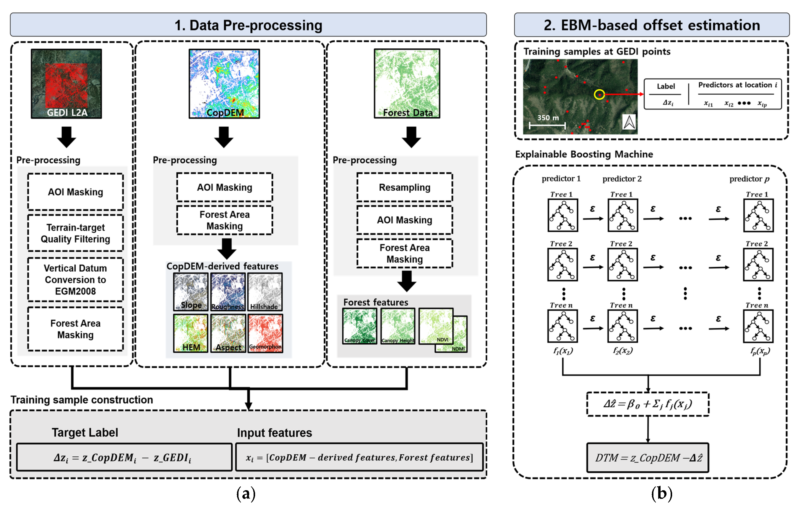
The elevation offset was first estimated with EBM and then used to generate the DTMs (Figure 3). For each grid cell, the elevation offset was defined as the difference between CopDEM and GEDI ground elevation and used as the prediction target:

Δz_i = z_CopDEM,i − z_GED,i

(1)

where z_CopDEM,i is the CopDEM elevation, z_GEDI,i is the GEDI L2A ground elevation, and Δz_i is the elevation offset for the i-th grid cell. The offset was estimated from the eleven predictors listed in Table 1.

Figure 3. Overall workflow of the proposed method: (a) GEDI filtering and preparation of the predictors listed in Table 1 to construct training samples; and (b) EBM-based estimation of the elevation offset and generation of the proposed DTM by subtracting the predicted offset from CopDEM.

3.2. Data Preparation

GEDI points were filtered based on the screening criteria proposed by Moudrý et al. [37] for terrain-elevation retrieval in temperate forests and grasslands. Previous studies in the Republic of Korea have similarly applied quality-based filtering to GEDI L2A data and adjusted the screening criteria to local forest conditions [38]. Only points satisfying quality_flag = 1, degrade_flag = 0, sensitivity ≥ 0.9, and one to four detected modes were retained. Points for which the lowest-mode elevation differed from the TanDEM-X 90 m DEM by more than 50 m were excluded. Moudrý et al. [37] proposed a 100 m threshold for forested areas, but a stricter threshold of 50 m was adopted in this study. This value removes unusually large elevation differences while still covering the range of canopy-related differences expected in Korean forests. In addition, only points for which the estimated elevations agreed within 2 m across algorithm setting groups were retained. Each criterion targets a different type of low-quality observation. The quality_flag criterion retains observations with valid waveform energy, amplitude, sensitivity, and surface-tracking quality, whereas the degrade_flag criterion excludes observations with degraded pointing or geolocation. The sensitivity threshold of 0.9 retains observations that are expected to detect the ground under canopy cover of up to 90% [37]. Limiting the number of detected modes to one to four reduces the risk of poor terrain-elevation accuracy caused by highly complex waveforms [37]. The elevation-difference and algorithm-agreement criteria remove anomalous ground-elevation estimates and those sensitive to processing settings. The sensitivity of the results to these criteria is examined in Appendix A. Each filtered GEDI point was then assigned to the CopDEM GLO-30 grid cell containing its center coordinate. When multiple GEDI points occurred within the same cell because of repeat tracks in the 2019–2025 dataset, the mean ground elevation was used. The resulting cell-level GEDI ground elevations were restricted to forested areas and used to calculate the elevation offsets.

3.3. Offset Estimation with an EBM

The EBM is an intrinsically interpretable generalized additive model that learns an independent shape function for each predictor and forms its prediction as their sum [23,24,25]. The offset is modeled in additive form as

$$\Delta \widehat{\mathrm{z}}={\beta }_0+\sum _j{f}_j\left(x_j\right)$$

(2)

where Δẑ is the estimated offset, β₀ is the intercept, and f_j is the shape function of predictor x_j. Each shape function is learned using shallow trees trained sequentially across predictors, allowing the contribution associated with each predictor to be examined directly.

The model was fitted with the ExplainableBoostingRegressor of InterpretML (v0.7.8) under an RMSE objective, using the offset in Equation (1) as the target and the eleven predictors as inputs. Pairwise interaction terms were disabled (interactions = 0) to keep the model purely additive and each predictor directly interpretable. The categorical geomorphon class was treated as nominal and the remaining predictors as continuous. The random seed was fixed (random_state = 42) for reproducibility, and the remaining settings were max_bins = 1024, max_leaves = 2, min_samples_leaf = 4, learning_rate = 0.04, outer_bags = 14, inner_bags = 0, max_rounds = 50,000 with early_stopping_rounds = 100, validation_size = 0.15, smoothing_rounds = 500, and greedy_ratio = 10.0. Model fitting and prediction were performed in Python 3.13.9. The fitted model was applied to every forested grid cell to predict the offset, which was subtracted from CopDEM to obtain the proposed DTM. This yields a continuous, ground-referenced terrain surface across the forested area of each study region, including cells without GEDI observations, and is expressed as

$$z_{\mathit{DTM}}=z_{\mathit{CopDEM}}-∆\widehat{z}$$

(3)

For the local-explanation analysis, cells were grouped into four environments by combining low and high canopy height with low and high slope, both derived from airborne LiDAR. Low was defined as values at or below the 50th percentile and high as values at or above the 75th percentile of the two regions combined with equal weight (canopy height: 11.3 and 13.8 m; slope: 21.8° and 27.7°). Cells between the two percentiles were excluded to keep the environments clearly separated. Because no GEDI training observation falls inside the airborne LiDAR coverage, every cell in this analysis is out-of-sample. Within each environment, the per-cell term contributions of the EBM were averaged and expressed as deviations from the region-wide mean contributions. For comparison, the mean reference offset (CopDEM-airborne LiDAR DTM) and the corresponding residual were also computed for each environment. The environments are classified by the airborne LiDAR canopy height, whereas the model input canopy height is the 2019 global canopy height product.

3.4. Accuracy Assessment

Accuracy was assessed using the RMSE, mean absolute error (MAE), bias, standard deviation (STD), and NMAD of the elevation differences between each evaluated surface and the airborne LiDAR DTM. These metrics were computed over forested cells in the airborne LiDAR extent where both surfaces were valid, as follows:

$$\mathrm{RMSE}=\sqrt{{\displaystyle \frac{1}{n}}\sum _{i=1}^n{\left({\widehat{y}}_i-y_i\right)}^2}$$

(4)

$$\mathrm{MAE}={\displaystyle \frac{1}{n}}\sum _{i=1}^n\left|{\widehat{y}}_i-y_i\right|$$

(5)

$$\mathrm{bias}={\displaystyle \frac{1}{n}}\sum _{i=1}^n\left({\widehat{y}}_i-y_i\right)$$

(6)

$$\mathrm{Standard}\mathrm{Deviation}=\sqrt{{\displaystyle \frac{1}{n}}\sum _{i=1}^n{\left[\left({\widehat{y}}_i-y_i\right)-\mathrm{bias}\right]}^2}$$

(7)

$$\mathrm{N}\mathrm{M}\mathrm{A}\mathrm{D}=1.4826·\mathrm{m}\mathrm{e}\mathrm{d}\mathrm{i}\mathrm{a}\mathrm{n}\left(\right|\Delta {\mathit{h}}_{\mathit{i}}-{\mathrm{m}}_{\Delta h}\left|\right)$$

(8)

where y_i is the airborne LiDAR DTM elevation of cell i, ${\widehat{y}}_i$ is the corresponding elevation of the proposed DTM, z_DTM from Equation (3), and n is the number of validation cells over which the metrics are computed. Since the airborne LiDAR data were excluded from training, this comparison is independent of model fitting. The same metrics were computed for CopDEM and the global bare-earth products FABDEM and GEDTM30, with ${\widehat{y}}_i$ replaced by the elevation of the respective product. In Equation (8), ∆h_i = ${\widehat{y}}_i-y_i$ denotes the elevation difference of cell i, m_∆h is the median of ∆h_i over all validation cells, and the factor 1.4826 makes the NMAD consistent with the standard deviation for normally distributed errors [19]. Uncertainty in the class-wise metrics was quantified by a spatial block bootstrap. Cells were grouped into 720 m blocks to account for spatial autocorrelation, and the blocks were resampled with replacement 1000 times. The 2.5th and 97.5th percentiles of the resulting distribution were taken as the 95% confidence interval. The difference between classes was regarded as distinguishable when its confidence interval excluded zero.

4. Results

4.1. Proposed Forest DTM

The proposed DTM was generated over the forested areas of both study regions (Figure 4). Its elevation and slope statistics were compared with those of CopDEM. After removal of the estimated offset, elevation decreased in 98.9% (central-western) and 99.6% (eastern) of the forested cells. Mean elevation decreased from 225 to 216 m (central-western) and from 428 to 417 m (eastern), with mean reductions of 9.1 and 10.9 m, and the elevation range changed from 8–866 to 2–863 m and from 0–1211 to −5–1210 m. Mean slope increased from 20° to 22° and from 21° to 24°, and the proportion of cells steeper than 25° rose from 26% to 36% and from 34% to 45%.

Figure 4. Proposed DTM over the two study regions: (a) the central-western region and (b) the eastern region, each shown over the 0.5° × 0.5° tile. The black boxes mark the detailed validation windows, denoted Site A in (a) and Site B in (b).

4.2. Accuracy Assessment Against Airborne LiDAR

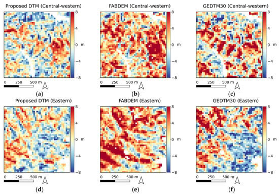
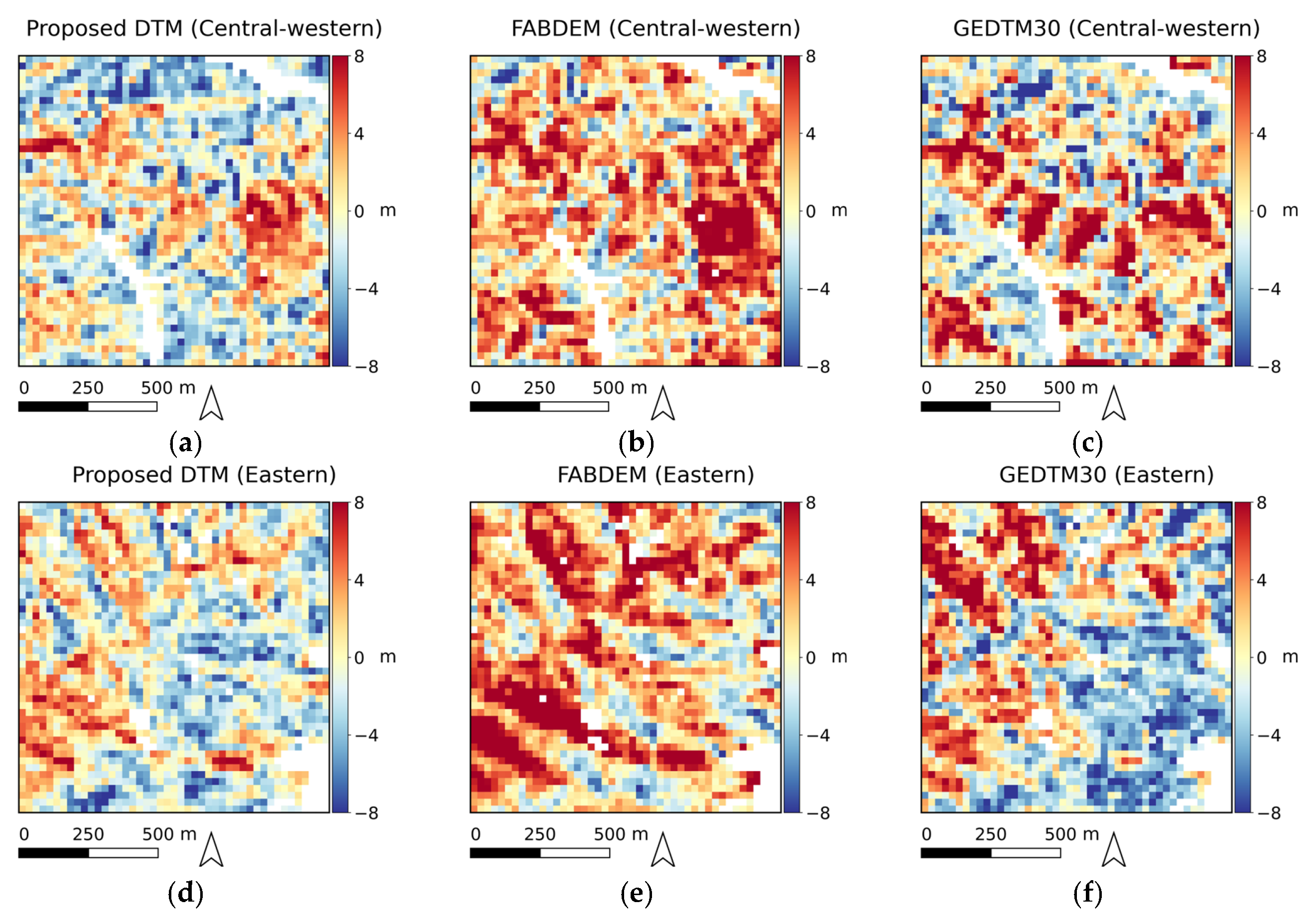
To examine local accuracy on demanding terrain, a detailed validation window of about 1.35 km × 1.35 km was selected in each region over steep forested terrain with slopes in the upper range of that region. These windows, Site A in the central-western region and Site B in the eastern region, are marked by the black boxes in Figure 4. The difference maps in Figure 5 (product minus airborne LiDAR DTM) show that the proposed DTM was closest to the reference at both sites.

Figure 5. Elevation difference from the airborne LiDAR DTM (product minus airborne LiDAR DTM) over the two detailed validation windows: (a–c) Site A in the central-western region and (d–f) Site B in the eastern region, showing (a,d) the proposed DTM, (b,e) FABDEM, and (c,f) GEDTM30. The shared color scale spans ±8 m; red indicates overestimation of the ground elevation and blue underestimation. White areas are cells without valid data on either surface.

Site A and Site B have slopes of about 28° and 29° and canopy heights of about 12 and 15 m, with 1925 and 1922 valid cells. Within Site A, the RMSE of the proposed DTM was 3.66 m, compared with 4.71 m for FABDEM and 4.93 m for GEDTM30. Within Site B, the corresponding values were 3.43, 4.95, and 4.71 m. The proposed DTM thus reduced the RMSE by 22% (Site A) and 31% (Site B) relative to FABDEM and by 26% and 27% relative to GEDTM30. The bias was −0.62 and −0.49 m for the proposed DTM, +2.59 and +2.72 m for FABDEM, and +1.20 and −0.44 m for GEDTM30.

Over the full airborne LiDAR extent of each region, the accuracy of the proposed DTM was compared with that of CopDEM and the two global bare-earth products, FABDEM and GEDTM30 (Table 2, Figure 6). Before correction, CopDEM showed a bias of +10.51 m (central-western) and +9.31 m (eastern) and an RMSE of 11.52 and 10.34 m. The RMSE of the proposed DTM (4.10 and 3.67 m) was lower than those of FABDEM (5.36 and 4.61 m) and GEDTM30 (5.17 and 4.66 m). The MAE showed the same pattern: 3.25 and 2.92 m for the proposed DTM, compared with 4.23 and 3.71 m for FABDEM and 4.05 and 3.76 m for GEDTM30.

Table 2. Accuracy of CopDEM, the proposed DTM, and the global bare-earth products (FABDEM, GEDTM30) against the airborne LiDAR DTM, computed over the same pixels within the airborne LiDAR extent.

Region	Product	Bias (m)	MAE (m)	RMSE (m)	STD (m)	NMAD (m)
Central-western	CopDEM	10.51	10.51	11.52	4.73	4.78
	Proposed DTM	0.57	3.25	4.10	4.06	4.01
	FABDEM	2.02	4.23	5.36	4.96	4.89
	GEDTM30	1.79	4.05	5.17	4.85	4.76
Eastern	CopDEM	9.31	9.31	10.34	4.50	4.64
	Proposed DTM	−0.88	2.92	3.67	3.56	3.54
	FABDEM	−0.09	3.71	4.61	4.61	4.71
	GEDTM30	−1.58	3.76	4.66	4.39	4.34

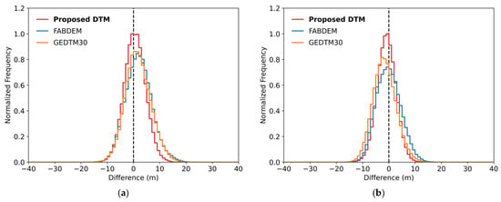
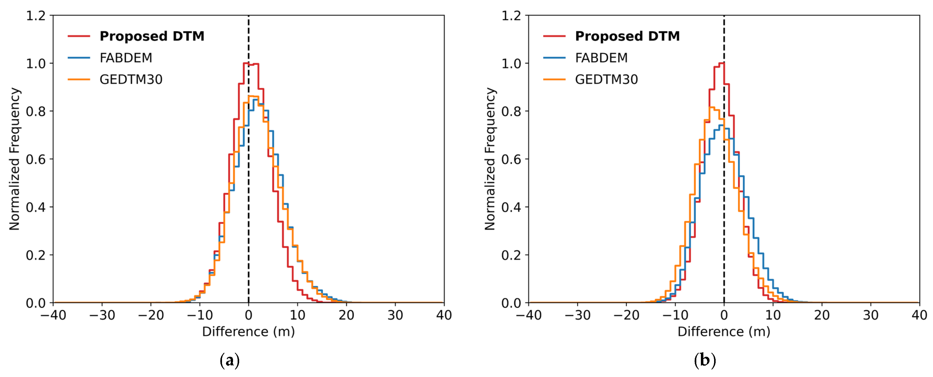
Figure 6. Peak-normalized error distributions (proposed DTM, FABDEM, and GEDTM30 minus the airborne LiDAR DTM) for (a) the central-western region and (b) the eastern region.

Figure 6 shows the error distributions of the proposed DTM, FABDEM, and GEDTM30, among which the distribution of the proposed DTM was the narrowest. The STD of the proposed DTM was 4.06 m (central-western) and 3.56 m (eastern), smaller than those of FABDEM (4.96 and 4.61 m), GEDTM30 (4.85 and 4.39 m), and CopDEM (4.73 and 4.50 m). The proposed DTM therefore reduced the dispersion relative to CopDEM in both regions, whereas FABDEM did not in either region and GEDTM30 did so only in the eastern region. The NMAD was also lowest for the proposed DTM (4.01 and 3.54 m), compared with 4.78 and 4.64 m for CopDEM, 4.89 and 4.71 m for FABDEM, and 4.76 and 4.34 m for GEDTM30. The bias of the proposed DTM was +0.57 and −0.88 m, within ±0.9 m in both regions, whereas the bias of FABDEM (+2.02 and −0.09 m) and GEDTM30 (+1.79 and −1.58 m) differed more between regions. FABDEM showed the largest single bias, a systematic overestimation of +2.02 m in the central-western region but was the least biased product in the eastern region.

4.3. Predictor Contributions to the Offset

Because EBM is additive, predictor contributions to the offset can be examined at three levels: the incremental contribution of predictor groups, the overall magnitude of each predictor (variable importance), and its signed contribution under specific terrain and canopy conditions (local explanations). The incremental contribution of the predictor groups was assessed by fitting the model to successively larger predictor sets and evaluating every fit over the same validation cells (Table 3). The topographic predictors alone gave an RMSE of 4.53 m (central-western) and 4.01 m (eastern). Each group reduced the error further when the other was already in the model. Adding the canopy-structure predictors to the topography and HEM set reduced the RMSE by 0.22 and 0.18 m, and adding HEM to the topography and canopy-structure set reduced it by 0.24 and 0.05 m. The RMSE was lowest for the full predictor set (4.10 and 3.67 m).

Table 3. Incremental contribution of the predictor groups to the accuracy of the proposed DTM. Topography comprises elevation, slope, aspect, roughness, hillshade, and geomorphon; canopy structure comprises canopy cover, canopy height, NDVI, and NDMI; HEM is the InSAR height error. ΔRMSE is the change from the topography-only model; negative values indicate improvement.

Predictor Set	No. of Predictors	Central-Western RMSE (m)	Central-Western ΔRMSE (m)	Eastern RMSE (m)	Eastern ΔRMSE (m)
Topography	6	4.53	0	4.01	0
Topography + HEM	7	4.32	−0.21	3.85	−0.16
Topography + canopy structure	10	4.34	−0.19	3.72	−0.29
Proposed	11	4.10	−0.4 3	3.67	−0.34

The importance of predictor j is defined as the mean absolute contribution of its shape function over the training data,

$$I_j={\displaystyle \frac{1}{N}}{\sum }_{i=1}^N\left|f_j\left(x_{\mathit{ij}}\right)\right|$$

(9)

where (f_jx_ij) is the contribution of predictor j for sample i (the score of the corresponding bin, in meters) and N is the number of training samples.

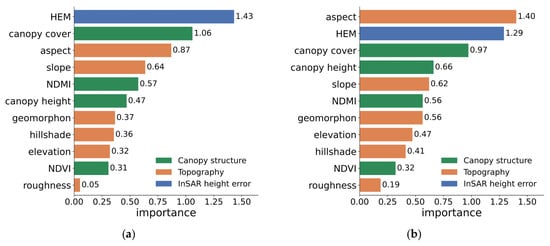
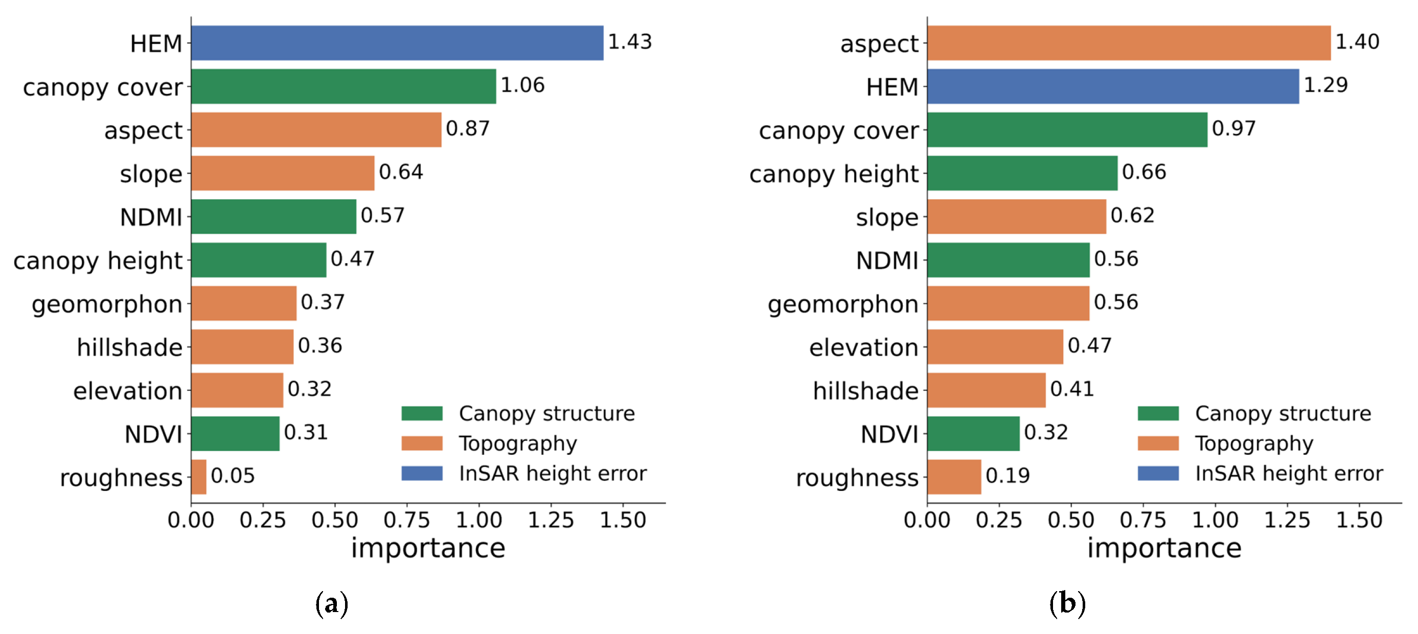
Figure 7 shows the variable importance for the two regions. Importance was concentrated in HEM, canopy cover, and aspect in both regions. In the central-western region, HEM ranked first (1.43 m), canopy cover second (1.06 m), and aspect third (0.87 m). In the eastern region, aspect ranked first (1.40 m), HEM second (1.29 m), and canopy cover third (0.97 m). The remaining predictors had importances below 0.7 m in both regions, with roughness the lowest (0.05 and 0.19 m).

Figure 7. EBM variable importance (mean absolute score) for (a) the central-western region and (b) the eastern region. Bars are colored by predictor group: canopy structure (green), topography (orange), and InSAR height error (blue).

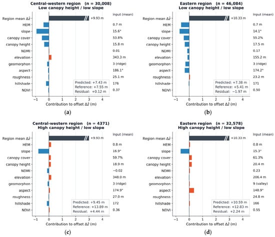
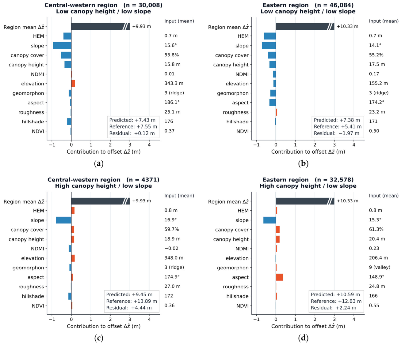
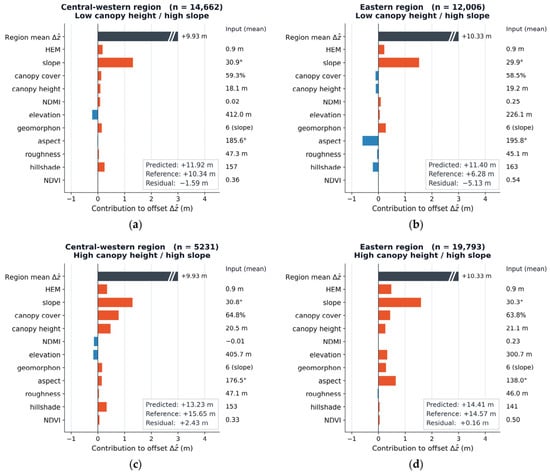
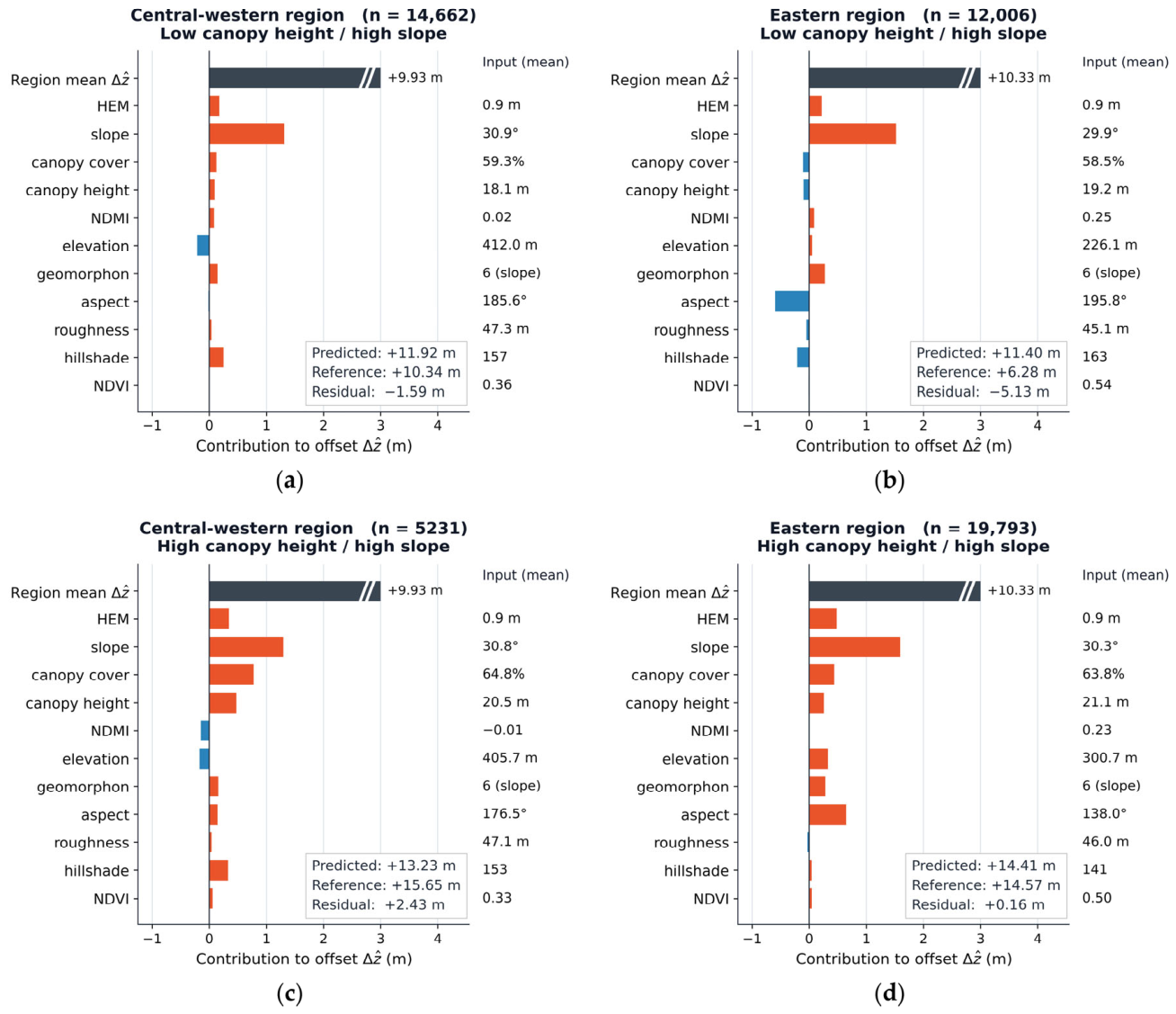
Figure 8 and Figure 9 show the mean local EBM contributions for the four canopy–slope environments. The region-mean predicted offset over the LiDAR-covered validation cells was +9.93 m (central-western) and +10.33 m (eastern). Several predictors showed relatively large deviations from their regional mean contributions, and three of them, slope, HEM, and the canopy variables, behaved consistently in both regions (Figure 8 for low slope and Figure 9 for high slope). Slope showed the largest deviation in every panel, contributing −0.6 to −0.9 m in the low-slope environments and +1.3 to +1.6 m in the high-slope environments. HEM was negative under low canopy on gentle terrain (−0.4 m central-western and −0.6 m eastern) and positive in the other three environments, reaching +0.3 to +0.5 m under high canopy on steep terrain. Canopy cover and canopy height followed a similar gradient in three of the four environments, from −0.3 to −0.5 m under low canopy on gentle terrain to +0.3 to +0.8 m under high canopy on steep terrain. The exception was low canopy on steep terrain, where both remained weakly positive in the central-western region (+0.13 m for canopy cover and +0.09 m for canopy height) and weakly negative in the eastern region (−0.13 and −0.14 m).

Figure 8. Environment-mean local EBM explanations for the central-western and eastern regions under low-slope conditions, stratified by canopy height: (a,b) low canopy height and low slope, and (c,d) high canopy height and low slope, with the central-western case on the left and the eastern case on the right of each pair. Each panel title gives the region, the environment, and the number of cells, and an inset box reports the predicted offset, the reference offset, and their difference (residual). The leading black bar, labeled Region mean Δẑ in the figure, is the region-mean predicted offset and extends beyond the plotted axis range; the predictor bars give the mean term contribution in that environment as a deviation from the region mean (orange positive, blue negative), and the values on the right give the corresponding mean input of each predictor. A positive contribution increases the estimated offset, and a negative contribution decreases it.

Figure 9. Environment-mean local EBM explanations for the central-western and eastern regions under high-slope conditions, stratified by canopy height: (a,b) low canopy height and high slope, and (c,d) high canopy height and high slope, with the central-western case on the left and the eastern case on the right of each pair. Each panel title gives the region, the environment, and the number of cells, and an inset box reports the predicted offset, the reference offset, and their difference (residual). The leading black bar, labeled Region mean $∆\widehat{z}$ in the figure, is the region-mean predicted offset and extends beyond the plotted axis range; the predictor bars give the mean term contribution in that environment as a deviation from the region mean (orange positive, blue negative), and the values on the right give the corresponding mean input of each predictor. A positive contribution increases the estimated offset, and a negative contribution decreases it.

The remaining topographic predictors were less consistent between regions. Under low canopy on gentle terrain, elevation contributed +0.18 m (central-western) and −0.15 m (eastern), and the signs were reversed on steep terrain. Hillshade also differed in sign between regions under low canopy on steep terrain (+0.25 and −0.20 m). Aspect differed mainly in magnitude, ranging from −0.3 to −0.6 m under low canopy to +0.4 to +0.7 m under high canopy (eastern), whereas it remained within ±0.15 m (central-western).

The residuals further identified the environmental conditions in which larger errors remained, as reported in the inset boxes of Figure 8 and Figure 9. A near-zero residual occurred under low canopy and low slope in the central-western region (+0.12 m) and under high canopy and high slope in the eastern region (+0.16 m). Under high-canopy conditions, positive mean residuals were observed in the central-western region (+4.4 m on gentle slopes and +2.4 m on steep slopes) and the eastern region (+2.2 m on gentle slopes), indicating that the predicted offsets were smaller than the corresponding reference offsets. In contrast, negative mean residuals were observed under low-canopy conditions in the eastern region (−2.0 m on gentle slopes and −5.1 m on steep slopes) and the central-western region (−1.6 m on steep slopes), indicating that the predicted offsets exceeded the reference offsets.

4.4. Residual Error Analysis Under Different Environmental Conditions

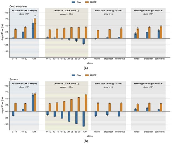
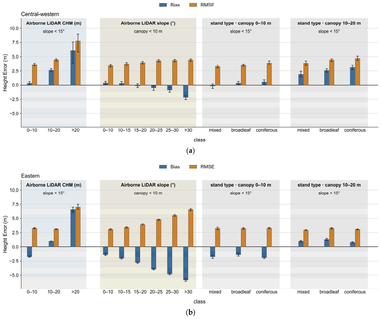
Figure 10 shows the residual errors of the proposed DTM under different canopy-height, slope, and forest-type conditions. For cells with slopes below 15°, bias shifted in the positive direction with increasing canopy height in both regions. From the 0–10 m to the 10–20 m canopy-height class, bias increased in the central-western region (from +0.22 to +2.58 m) and the eastern region (from −1.86 to +0.95 m). Above 20 m, positive biases were observed in the central-western region (+6.1 m) and the eastern region (+6.6 m). However, the central-western class contained only 27 cells, compared with 237 cells in the eastern region, and its bias therefore had a wide 95% confidence interval.

Figure 10. Elevation error of the proposed DTM (proposed DTM minus airborne LiDAR DTM) stratified by terrain and canopy variables derived independently from the airborne LiDAR data, for (a) the central-western and (b) the eastern region. Within each panel, cells are stratified by airborne LiDAR canopy height with slope controlled to <15°, by airborne LiDAR slope with canopy height controlled to <10 m, and by forest stand type within the 0–10 m and 10–20 m canopy-height bands on slopes <15°. Blue bars give the bias, and orange bars the RMSE of each class, with 95% confidence intervals estimated by a bootstrap over 720 m spatial blocks.

For cells with canopy heights below 10 m, bias shifted in the negative direction with increasing slope in both regions. From slopes below 10° to slopes above 30°, bias decreased in the central-western region (from +0.31 to −2.33 m) and the eastern region (from −1.59 to −5.99 m), and RMSE increased in the central-western region (from 3.35 to 4.59 m) and the eastern region (from 3.31 to 6.63 m). The eastern region generally showed a more negative bias than the central-western region.

Within slopes below 15°, differences among forest types were relatively small when canopy height was controlled by class. The range of bias among coniferous, broadleaf, and mixed forests was 0.73 m in the central-western region and 0.62 m in the eastern region in the 0–10 m canopy-height class, and 1.21 m and 0.53 m in the 10–20 m class. The relative ordering of bias among forest types also differed between regions. Coniferous forest showed the highest bias in both canopy-height classes in the central-western region (+0.57 m and +3.18 m), whereas it showed the lowest bias in the eastern region (−1.97 m and +0.78 m). Because these values were obtained under specified canopy-height and slope conditions, they represent relative differences among classes within each analysis and are not directly comparable with the overall regional bias from the full validation dataset.

5. Discussion

5.1. Accuracy Relative to the Input CopDEM and Global Bare-Earth Products

Compared with the input CopDEM, the proposed correction reduced the bias and the RMSE in both study regions, and the STD and NMAD also decreased. The bias decreased from +10.51 m (central-western) and +9.31 m (eastern) to +0.57 and −0.88 m, and the RMSE from 11.52 and 10.34 m to 4.10 and 3.67 m (Table 2). These results indicate that the proposed correction reduced the mean elevation difference and also partly reduced the dispersion of the pixel-wise elevation differences.

When compared over the same validation areas against the same independent airborne LiDAR reference, the proposed DTM showed lower RMSEs than FABDEM and GEDTM30 in both study regions (Table 2, Figure 6). In addition, the bias of the proposed DTM remained within ±0.9 m in both regions, whereas the bias of FABDEM and GEDTM30 differed in magnitude and direction between the regions. These results indicate that the accuracy of bare-earth elevation products developed at the global scale can vary with regional forest and terrain conditions [15,17].

However, these differences in accuracy should be interpreted in view of the differences in training data, predictor composition, modeling method, and spatial training extent among the products. FABDEM was developed for global application on the basis of reference elevation data from a wide range of regions [15], whereas GEDTM30 applied a global-to-local framework that combines a global model trained on globally distributed GEDI and ICESat-2 observations with local refinement at the 5° × 5° tile scale [17]. In contrast, the EBM in this study was trained separately using the GEDI observations selected within each 0.5° × 0.5° study region. The relatively lower RMSE obtained in this study therefore does not indicate the superiority of the EBM algorithm itself; it is more appropriately interpreted as the regional difference in accuracy among elevation products generated from different training data and modeling strategies, when evaluated against the same independent reference. In particular, because GEDTM30 also includes local refinement, this comparison is not simply one between a local and a global model. Moreover, because pixel-wise elevation differences remain after the correction, the overall accuracy assessment should be complemented by an analysis of how the elevation error varies with canopy height, terrain slope, and forest type, in order to identify the environmental conditions under which the correction is insufficient or excessive.

5.2. Interpretation of Predictor Contributions to the Elevation Offset

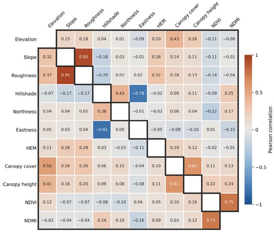
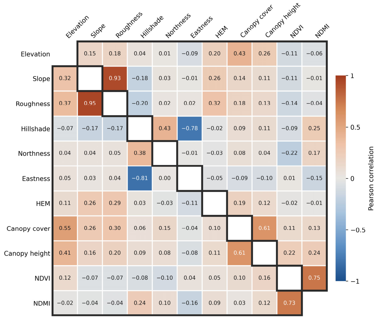
When related predictors are used together in an additive model, the effect of an individual model term may be difficult to interpret as completely independent of the other predictors [39]. Therefore, to account for relationships among predictors when interpreting the EBM contributions, Pearson correlation analysis was performed using the model-training data from the two study regions (Figure 11). Slope and roughness showed strong positive correlations, with r = 0.95 (central-western) and 0.93 (eastern), whereas hillshade and eastness showed strong negative correlations of r = −0.81 and −0.78. Among the forest-related predictors, canopy cover and canopy height were correlated at r = 0.61 in both regions, while NDVI and NDMI showed correlations of r = 0.73 (central-western) and 0.75 (eastern).

Figure 11. Pearson correlation matrix of the predictors used for model training in the central-western and eastern regions. The lower and upper triangles,delineated by black outlines,represent the central-western and eastern regions, respectively,and the blank diagonal cells indicate self-correlations. Because aspect is a circular variable, it was decomposed into northness (cos(θ)) and eastness (sin(θ)), where θ is the aspect angle in radians. Geomorphon was excluded from the correlation analysis because it is a categorical predictor.

In contrast, HEM showed generally weak correlations with the forest- and terrain-related predictors. Its correlations with canopy cover were r = 0.10 (central-western) and 0.19 (eastern), and those with canopy height were r = 0.11 and 0.12. Among the terrain predictors, the highest correlations were observed with roughness, at r = 0.29 and 0.32. HEM can therefore be regarded as a relatively independent predictor within the predictor set used in this study, with limited correlation with the other forest- and terrain-related predictors, and its large EBM contribution is unlikely to result from strong redundancy with any single predictor. However, because the canopy-related datasets and the TanDEM-X observations underlying CopDEM were acquired at different times, this temporal difference should also be considered when interpreting the relationships between HEM and the forest-related predictors.

These differences in predictor correlations indicate that predictor importance should be interpreted by considering both the relationships among predictors and the environmental conditions under which their contributions occur. In this study, the local explanations were used to examine both the magnitude and sign of predictor contributions under different environmental conditions, thereby allowing the elevation correction to be evaluated in terms of how it was composed from multiple sources of input information.

Using the currently available datasets, this study quantitatively characterized predictor contributions and predictor–offset relationships. However, the use of datasets acquired at different times and the limited availability of detailed acquisition information, such as the look direction and local incidence geometry of individual TanDEM-X acquisitions, should be considered when interpreting the physical meaning of these relationships in greater detail. Future analyses incorporating temporally better-matched optical and SAR satellite observations, more detailed acquisition-geometry information, and independent LiDAR-based canopy-structure data could further distinguish the contributions associated with forest structure and terrain conditions and provide a more detailed physical interpretation of the predictor–offset relationships identified in this study.

5.3. Residual Errors Under Different Environmental Conditions

Independent validation against the airborne LiDAR DTM showed that the bias shifted in the positive direction with increasing canopy height in both study regions. Under tall canopy, the proposed DTM was therefore higher than the reference ground, indicating that the offset estimated by the EBM was smaller than the correction actually required. Dong et al. [40] likewise reported, in a DSM-to-DTM reconstruction study, that the positive bias after correction increased in the taller canopy-height classes. This shows that a positive elevation bias can remain under tall canopy even after ground-elevation correction. The positive residuals observed in this study may have been influenced by uncertainty in both the predictors used for offset estimation and the GEDI ground-elevation estimates. Although the canopy height, canopy cover, and spectral variables used in this study represent the main characteristics of the forest, satellite remote sensing data alone cannot fully represent the vertical and horizontal structure of complex forest canopies in the predictors, and this limitation may have affected the estimation of the offset under tall canopy. Previous evaluations of GEDI ground elevation have also reported an increasing positive bias with increasing canopy height [41]. When GEDI ground elevation is overestimated, the CopDEM–GEDI elevation difference used for training becomes relatively small, and this bias may therefore also have contributed to the offset estimated by the EBM. The positive residuals under tall canopy may thus result from the combined effects of the range of canopy structure represented by the predictors and the uncertainty of the GEDI ground-elevation estimates. However, because the influence of each factor was not evaluated separately in this study, the dominant cause cannot be identified.

In contrast, the bias shifted in the negative direction with increasing terrain slope, and RMSE also increased in both study regions. This indicates that, on steep terrain, the offset estimated by the EBM was relatively larger than the actual elevation difference between CopDEM and the reference ground. Dong et al. [40] also reported a negative bias in the steepest slope class of their reconstructed DTM. In interpreting this tendency toward over-correction, the slope dependence of GEDI ground-elevation estimates should be considered. Shen et al. [42] compared GEDI ground elevation with the median airborne LiDAR DTM elevation within the footprint and reported that the mean difference changed from +2.20 m on slopes below 15° to −4.63 m on slopes above 35°, indicating that, on steep terrain, GEDI ground elevation may reflect relatively low terrain elevations within the footprint. When GEDI ground elevation is lower than the reference ground, the CopDEM–GEDI elevation difference used for training can become relatively large, and this characteristic may have affected the offset estimated by the EBM. In addition, the horizontal geolocation error of GEDI and the elevation variation within the approximately 25 m footprint can increase the uncertainty of ground-elevation estimates on steep terrain [37,43,44]. Because the bias of GEDI ground elevation and the error of the offset estimated by the EBM were not evaluated separately in this study, the dominant cause of the over-correction on steep terrain cannot be identified. The larger changes in negative bias and RMSE in the eastern region indicate that the magnitude of the residuals can also vary with regional terrain conditions.

Differences in residual error among forest types were relatively small compared with those associated with canopy height and terrain slope. Even after canopy height and slope were controlled, the mean residuals of coniferous, broadleaf, and mixed forests did not show a consistent order between the two regions. Li et al. [45] reported that the performance of DEM correction varies among forest types and that the forest types of the training data and of the corrected area affect the correction results. In this study, residual changes with canopy height and slope appeared more consistently in both regions than differences among forest types. This does not imply that forest type has no effect on elevation accuracy; rather, it indicates that, after canopy height and slope were taken into account, the additional residual differences among forest types were relatively small.

This analysis of residuals by environmental condition provides important information for characterizing the errors of the proposed DTM in detail. The largest positive bias occurred under tall canopy on gentle slopes and the largest negative bias under low canopy on steep slopes (Section 4.4). In actual forested terrain, multiple environmental conditions such as canopy height, terrain slope, and forest type act together, and their effects are jointly reflected in the residuals of the final DTM. By analyzing the residuals separately by environmental condition, this study identified changes in the magnitude and direction of the error with canopy height and slope that are difficult to detect from the overall accuracy assessment alone. However, this analysis evaluated the relationships between each environmental condition and the residuals and did not fully separate and quantify the influence of individual factors. In addition, the residual analysis used canopy height and slope derived from airborne LiDAR, and whether the same results would be obtained with the global canopy height product and CopDEM-derived slope was not examined. Future work should develop an error model based on these condition-specific residual characteristics and a pixel-level uncertainty map using globally available data.

5.4. Limitations

Several limitations should be considered when interpreting the results of this study. First, the input datasets differ in acquisition period: the TanDEM-X observations underlying CopDEM were acquired from 2011 to 2015, the GEDI observations span 2019–2025, NDVI and NDMI were derived from 2011 imagery, GFCC canopy cover represents 2015, the canopy height layer represents 2019, and the airborne LiDAR surveys were conducted in 2023 (central-western) and 2019 (eastern). Because ground elevation remains largely unchanged in the absence of terrain modification, these differences mainly affect areas where the forest canopy changed relative to the TanDEM-X acquisition period. To evaluate this effect, the validation cells were stratified by the year of forest loss in the Global Forest Change dataset (v1.12) [46]. Cells with no recorded loss accounted for 90.6% of the validation cells in the central-western region and 97.6% in the eastern region (Table 4). In cells where loss occurred, the RMSE of the proposed DTM increased to 4.57–5.91 m in the central-western region and 4.09–5.14 m in the eastern region, compared with 3.97 and 3.64 m in cells without loss. Because these cells account for only a small proportion of the validation cells, excluding all cells with loss since 2011 changed the RMSE only from 4.10 to 3.99 m in the central-western region and from 3.67 to 3.65 m in the eastern region, indicating that the regional accuracy is only weakly affected by stand-replacing forest loss, although errors are locally larger where such loss occurred.

Table 4. RMSE and bias (in parentheses) of the proposed DTM, FABDEM, and GEDTM30 by forest-loss period in the Global Forest Change dataset [46], relative to the TanDEM-X acquisition period (2011–2015). The proportion of validation cells in each class is given for each region. Values are in meters.

Loss Period	Central-Western				Eastern
	Cells (%)	Proposed DTM	FABDEM	GEDTM30	Cells (%)	Proposed DTM	FABDEM	GEDTM30
No loss	90.6	3.97 (+0.49)	4.99 (+1.91)	5.00 (+1.72)	97.6	3.64 (−0.87)	4.58 (−0.10)	4.64 (−1.59)
2001–2010 (before)	1.8	4.57 (−3.13)	6.14 (−5.27)	4.90 (−3.62)	0.2	5.14 (−3.36)	5.35 (−2.26)	4.68 (−2.46)
2011–2015 (during)	2.1	5.91 (+0.79)	7.32 (+1.77)	6.05 (+1.00)	0.9	4.97 (−2.00)	5.74 (−1.40)	6.02 (−3.33)
2016–2024 (after)	5.5	4.99 (+2.91)	8.83 (+6.33)	7.26 (+4.97)	1.3	4.09 (+0.05)	5.87 (+1.62)	5.08 (+0.22)
All	100	4.10 (+0.57)	5.36 (+2.02)	5.17 (+1.79)	100	3.67 (−0.88)	4.61 (−0.09)	4.66 (−1.58)

Where forest loss occurred, the bias shifted systematically with its timing (Table 4). In cells where the forest was lost after the TanDEM-X acquisitions (2016–2024), the bias shifted in the positive direction relative to cells without loss, consistent with CopDEM still representing the pre-loss canopy. In contrast, it shifted in the negative direction in cells lost before the acquisitions (2001–2010), where regrowth may have occurred. The same pattern was observed for FABDEM and GEDTM30, indicating that it arises from the acquisition timing of the underlying CopDEM rather than from the correction method. In cells lost during the acquisition period (2011–2015), the direction of the shift was not consistent across regions and products, suggesting that CopDEM may reflect a mixture of pre- and post-loss conditions. However, the forest loss data primarily capture stand-replacing disturbances, and thinning, partial harvesting, and gradual regrowth were not resolved; their effects on the correction therefore could not be evaluated separately.

Second, the analysis was conducted in two temperate forest regions in the Republic of Korea. The similar directions of the canopy-height- and slope-related residual changes in the two regions show that these patterns were repeatedly observed within the present study. However, aspect, elevation, and several other topographic predictors showed regional differences in their contributions. Forests in other environments, including boreal and tropical forests, may also differ substantially in canopy structure and X-band penetration characteristics. The predictor contributions and residual patterns identified here should therefore not be assumed to apply directly to other forest environments. Independent validation and, where necessary, model retraining would be required when applying the approach to new regions.

Third, the independent airborne LiDAR validation covered only part of each DTM production area. The forested validation areas covered approximately 73 km² in the central-western region and 160 km² in the eastern region, and their terrain and forest conditions do not necessarily represent the full range of conditions within the two 0.5° × 0.5° study regions. The reported RMSE, bias, and environment-specific residual patterns should therefore be interpreted as accuracy estimates for the LiDAR-covered validation areas rather than as direct estimates for all conditions across the entire DTM production areas.

Fourth, the number of validation cells was limited under some extreme environmental conditions. In particular, the canopy-height class above 20 m contained only 27 cells in the central-western region and consequently had a wide 95% confidence interval. The large positive bias observed in this class indicates the possibility of increased residual error under tall canopy, but its exact magnitude cannot be generalized with confidence. Further validation using independent airborne LiDAR data covering a wider range of canopy heights and terrain slopes would help characterize errors under these less well represented conditions.

6. Conclusions

This study generated a spatially continuous forest DTM by defining the difference between CopDEM and GEDI L2A ground elevation as an elevation offset, estimating the offset from terrain and forest variables using EBM, and subtracting the predicted offset from CopDEM. Validation against an independent airborne LiDAR DTM yielded RMSEs of 4.10 m in the central-western region and 3.67 m in the eastern region, lower than those of FABDEM and GEDTM30 over the same validation areas. Bias was +0.57 m in the central-western region and −0.88 m in the eastern region. This comparison represents the accuracy obtained by the region-specific modeling framework relative to products developed with broader spatial training extents, evaluated against the same independent reference. These results demonstrate that spatially discrete GEDI ground-elevation observations can be combined with spatially continuous global elevation and environmental data to generate continuous forest DTMs.

The additive structure of the EBM enabled the magnitude and direction of individual predictor contributions to the elevation offset to be examined directly while the offset was being modeled. HEM and canopy cover showed high importance in both regions, while aspect showed a particularly strong contribution in the eastern region. Local slope contributions followed a relatively consistent direction in the two regions, whereas aspect and several other topographic predictors showed stronger regional differences. Independent residual analysis based on airborne LiDAR showed that bias shifted in the positive direction with increasing canopy height and in the negative direction with increasing slope, with the slope-related increase in error being particularly pronounced in the eastern region. These systematic residual patterns indicate that the proposed DTM should be used with caution under tall canopy and on steep slopes, and that canopy height and slope can serve as criteria for identifying areas of lower expected accuracy. In contrast, differences in residual error among forest types were relatively small and showed no consistent ordering between the two regions after canopy height and slope were controlled.

The main contribution of this study is therefore not only the generation of a continuous forest DTM through correction of the CopDEM elevation offset, but also the use of an interpretable additive model to quantify how the correction is related to terrain and forest conditions and to identify the environmental conditions under which residual errors increase. The approach provides a potential means of producing continuous forest DTMs in regions where airborne LiDAR is unavailable by combining GEDI with globally available remote-sensing data. However, the present validation was limited to two temperate forest regions in the Republic of Korea. Future work should therefore evaluate the approach across a wider range of forest and terrain environments, including boreal and tropical forests. Improved waveform and geolocation quality control for GEDI ground elevations on steep terrain, together with forest-structure variables that better represent structural variation under tall canopy, may further reduce the residual errors identified in this study. In addition, the class-specific errors reported here provide a basis for developing a pixel-level uncertainty layer that accompanies the DTM.

References

- Guth, P.L.; Van Niekerk, A.; Grohmann, C.H.; Muller, J.-P.; Hawker, L.; Florinsky, I.V.; Gesch, D.; Reuter, H.I.; Herrera-Cruz, V.; Riazanoff, S.; et al. Digital elevation models: Terminology and definitions. Remote Sens. 2021, 13, 3581. [Google Scholar] [CrossRef] [Scilit]
- Lefsky, M.A.; Cohen, W.B.; Parker, G.G.; Harding, D.J. Lidar remote sensing for ecosystem studies. BioScience 2002, 52, 19–30. [Google Scholar] [CrossRef] [Scilit]
- Clark, M.L.; Clark, D.B.; Roberts, D.A. Small-footprint lidar estimation of sub-canopy elevation and tree height in a tropical rain forest landscape. Remote Sens. Environ. 2004, 91, 68–89. [Google Scholar] [CrossRef] [Scilit]
- Rosen, P.A.; Hensley, S.; Joughin, I.R.; Li, F.K.; Madsen, S.N.; Rodriguez, E.; Goldstein, R.M. Synthetic aperture radar interferometry. Proc. IEEE 2000, 88, 333–382. [Google Scholar] [CrossRef] [Scilit]
- Rizzoli, P.; Martone, M.; Gonzalez, C.; Wecklich, C.; Borla Tridon, D.; Bräutigam, B.; Bachmann, M.; Schulze, D.; Fritz, T.; Huber, M.; et al. Generation and performance assessment of the global TanDEM-X digital elevation model. ISPRS J. Photogramm. Remote Sens. 2017, 132, 119–139. [Google Scholar] [CrossRef] [Scilit]
- Ziemer, J.; Dubois, C.; Thiel, C.; Bueso-Bello, J.-L.; Rizzoli, P.; Schmullius, C. Relationship between lidar-derived canopy densities and the scattering phase center of high-resolution TanDEM-X data. Remote Sens. 2023, 15, 3589. [Google Scholar] [CrossRef] [Scilit]
- Schlund, M.; Baron, D.; Magdon, P.; Erasmi, S. Canopy penetration depth estimation with TanDEM-X and its compensation in temperate forests. ISPRS J. Photogramm. Remote Sens. 2019, 147, 232–241. [Google Scholar] [CrossRef] [Scilit]
- Collins, J.; Riegler, G.; Schrader, H.; Tinz, M. Applying terrain and hydrological editing to TanDEM-X data to create a consumer-ready WorldDEM product. Int. Arch. Photogramm. Remote Sens. Spat. Inf. Sci. 2015, XL-7/W3, 1149–1154. [Google Scholar] [CrossRef] [Scilit]
- Airbus Defence and Space GmbH. Copernicus Digital Elevation Model: Product Handbook, Version 5.0 ed.; Document GEO1988-COPERNICUSDEM-SPE-002; Airbus Defence and Space GmbH: Ottobrunn, Germany, 2022; Available online: https://dataspace.copernicus.eu (accessed on 1 May 2026).
- Hyyppä, J.; Hyyppä, H.; Leckie, D.; Gougeon, F.; Yu, X.; Maltamo, M. Review of methods of small-footprint airborne laser scanning for extracting forest inventory data in boreal forests. Int. J. Remote Sens. 2008, 29, 1339–1366. [Google Scholar] [CrossRef] [Scilit]
- Reutebuch, S.E.; McGaughey, R.J.; Andersen, H.-E.; Carson, W.W. Accuracy of a high-resolution lidar terrain model under a conifer forest canopy. Can. J. Remote Sens. 2003, 29, 527–535. [Google Scholar] [CrossRef] [Scilit]
- Wulder, M.A.; White, J.C.; Nelson, R.F.; Næsset, E.; Ørka, H.O.; Coops, N.C.; Hilker, T.; Bater, C.W.; Gobakken, T. Lidar sampling for large-area forest characterization: A review. Remote Sens. Environ. 2012, 121, 196–209. [Google Scholar] [CrossRef] [Scilit]
- Dubayah, R.; Blair, J.B.; Goetz, S.; Fatoyinbo, L.; Hansen, M.; Healey, S.; Hofton, M.; Hurtt, G.; Kellner, J.; Luthcke, S.; et al. The Global Ecosystem Dynamics Investigation: High-resolution laser ranging of the Earth’s forests and topography. Sci. Remote Sens. 2020, 1, 100002. [Google Scholar] [CrossRef] [Scilit]
- Yamazaki, D.; Ikeshima, D.; Tawatari, R.; Yamaguchi, T.; O’Loughlin, F.; Neal, J.C.; Sampson, C.C.; Kanae, S.; Bates, P.D. A high-accuracy map of global terrain elevations. Geophys. Res. Lett. 2017, 44, 5844–5853. [Google Scholar] [CrossRef] [Scilit]
- Hawker, L.; Uhe, P.; Paulo, L.; Sosa, J.; Savage, J.; Sampson, C.; Neal, J. A 30 m global map of elevation with forests and buildings removed. Environ. Res. Lett. 2022, 17, 024016. [Google Scholar] [CrossRef] [Scilit]
- Laipelt, L.; Comini de Andrade, B.; Collischonn, W.; de Amorim Teixeira, A.; de Paiva, R.C.D.; Ruhoff, A. ANADEM: A digital terrain model for South America. Remote Sens. 2024, 16, 2321. [Google Scholar] [CrossRef] [Scilit]
- Ho, Y.-F.; Grohmann, C.H.; Lindsay, J.; Reuter, H.I.; Parente, L.; Witjes, M.; Hengl, T. GEDTM30: Global ensemble digital terrain model at 30 m and derived multiscale terrain variables. PeerJ 2025, 13, e19673. [Google Scholar] [CrossRef] [Scilit]
- Gdulová, K.; Marešová, J.; Moudrý, V. Accuracy assessment of the global TanDEM-X digital elevation model in a mountain environment. Remote Sens. Environ. 2020, 241, 111724. [Google Scholar] [CrossRef] [Scilit]
- Uuemaa, E.; Ahi, S.; Montibeller, B.; Muru, M.; Kmoch, A. Vertical accuracy of freely available global digital elevation models (ASTER, AW3D30, MERIT, TanDEM-X, SRTM, and NASADEM). Remote Sens. 2020, 12, 3482. [Google Scholar] [CrossRef] [Scilit]
- Meadows, M.; Jones, S.; Reinke, K. Vertical accuracy assessment of freely available global DEMs (FABDEM, Copernicus DEM, NASADEM, AW3D30 and SRTM) in flood-prone environments. Int. J. Digit. Earth 2024, 17, 2308734. [Google Scholar] [CrossRef] [Scilit]
- Aati, S.; Avouac, J.-P. Optimization of optical image geometric modeling, application to topography extraction and topographic change measurements using PlanetScope and SkySat imagery. Remote Sens. 2020, 12, 3418. [Google Scholar] [CrossRef] [Scilit]
- Okolie, C.; Mills, J.; Adeleke, A.; Smit, J. Digital elevation model correction in urban areas using extreme gradient boosting, land cover and terrain parameters. Int. Arch. Photogramm. Remote Sens. Spat. Inf. Sci. 2024, XLVIII-4/W9-2024, 275–282. [Google Scholar] [CrossRef] [Scilit]
- Lou, Y.; Caruana, R.; Gehrke, J.; Hooker, G. Accurate intelligible models with pairwise interactions. In Proceedings of the 19th ACM SIGKDD International Conference on Knowledge Discovery and Data Mining, Chicago, IL, USA, 11–14 August 2013; pp. 623–631. [Google Scholar] [CrossRef] [Scilit]
- Nori, H.; Jenkins, S.; Koch, P.; Caruana, R. InterpretML: A unified framework for machine learning interpretability. arXiv 2019, arXiv:1909.09223. [Google Scholar]
- Nori, H.; Caruana, R.; Bu, Z.; Shen, J.H.; Kulkarni, J. Accuracy, interpretability, and differential privacy via explainable boosting. In Proceedings of the 38th International Conference on Machine Learning, Virtual, 18–24 July 2021; Volume PMLR 139, pp. 8227–8237. [Google Scholar]
- Korea Forest Service. Forest Spatial Information Service: National Forest-Type Map. Available online: https://map.forest.go.kr/ (accessed on 1 May 2026).
- European Space Agency. Copernicus Global Digital Elevation Model. OpenTopography 2024. [Google Scholar] [CrossRef]
- Jasiewicz, J.; Stepinski, T.F. Geomorphons—A pattern recognition approach to classification and mapping of landforms. Geomorphology 2013, 182, 147–156. [Google Scholar] [CrossRef] [Scilit]
- Sexton, J.O.; Song, X.-P.; Feng, M.; Noojipady, P.; Anand, A.; Huang, C.; Kim, D.-H.; Collins, K.M.; Channan, S.; DiMiceli, C.; et al. Global, 30-m resolution continuous fields of tree cover: Landsat-based rescaling of MODIS Vegetation Continuous Fields with lidar-based estimates of error. Int. J. Digit. Earth 2013, 6, 427–448. [Google Scholar] [CrossRef] [Scilit]
- Potapov, P.; Li, X.; Hernandez-Serna, A.; Tyukavina, A.; Hansen, M.C.; Kommareddy, A.; Pickens, A.; Turubanova, S.; Tang, H.; Silva, C.E.; et al. Mapping global forest canopy height through integration of GEDI and Landsat data. Remote Sens. Environ. 2021, 253, 112165. [Google Scholar] [CrossRef] [Scilit]
- Rouse, J.W.; Haas, R.H.; Schell, J.A.; Deering, D.W. Monitoring vegetation systems in the Great Plains with ERTS. In Proceedings of the Third ERTS Symposium; NASA SP-351; NASA: Washington, DC, USA, 1974; pp. 309–317. [Google Scholar]
- Wilson, E.H.; Sader, S.A. Detection of forest harvest type using multiple dates of Landsat TM imagery. Remote Sens. Environ. 2002, 80, 385–396. [Google Scholar] [CrossRef] [Scilit]
- U.S. Geological Survey. Landsat 7. Available online: https://www.usgs.gov/landsat-missions/landsat-7 (accessed on 1 July 2025).
- Roy, D.P.; Kovalskyy, V.; Zhang, H.K.; Vermote, E.F.; Yan, L.; Kumar, S.S.; Egorov, A. Characterization of Landsat-7 to Landsat-8 reflective wavelength and normalized difference vegetation index continuity. Remote Sens. Environ. 2016, 185, 57–70. [Google Scholar] [CrossRef] [Scilit]
- Kim, D.-E.; Oh, J.-S. Landform classification using geomorphons on the Middle Yangsan Fault System, southeastern Korea. J. Korean Geogr. Soc. 2019, 54, 493–505. [Google Scholar]
- Cheon, Y.; Ha, S.; Kim, D.-E.; Ryoo, C.-R. The nature and structural-geomorphic characteristics of the Gyeryongsan Fault, central Korea. J. Geol. Soc. Korea 2026, 62, 373–383. [Google Scholar] [CrossRef] [Scilit]
- Moudrý, V.; Prošek, J.; Marselis, S.; Marešová, J.; Šárovcová, E.; Gdulová, K.; Kozhoridze, G.; Torresani, M.; Rocchini, D.; Eltner, A.; et al. How to find accurate terrain and canopy height GEDI footprints in temperate forests and grasslands? Earth Space Sci. 2024, 11, e2024EA003709. [Google Scholar] [CrossRef] [Scilit]
- Lee, S.; Lee, M.J. Forest aboveground biomass estimation by the integration of GEDI LiDAR and national forest inventory data in South Korea. Korean J. Remote Sens. 2025, 41, 407–419. [Google Scholar] [CrossRef] [Scilit]
- Ramsay, T.O.; Burnett, R.T.; Krewski, D. The effect of concurvity in generalized additive models linking mortality to ambient particulate matter. Epidemiology 2003, 14, 18–23. [Google Scholar] [CrossRef] [Scilit]
- Dong, J.; Hu, J.; Gui, R.; Yuan, Y.; Qin, Y.; Mo, Z. DSM-to-DTM reconstruction using only DSM-derived inputs with residual learning and CSF priors. Remote Sens. 2026, 18, 1625. [Google Scholar] [CrossRef] [Scilit]
- Cățeanu, M. Evaluating the accuracy of ground elevation estimates from GEDI satellite LiDAR in forested terrain. Geo-Spat. Inf. Sci. 2026, 29, 2043–2061. [Google Scholar] [CrossRef] [Scilit]
- Shen, F.; He, X.; Gu, Y.; Qin, Z.; Wu, X. Diagnosing GEDI canopy height errors in steep mountainous forests: Ground elevation representation and geolocation uncertainty. Forests 2026, 17, 1087. [Google Scholar] [CrossRef] [Scilit]
- Adam, M.; Urbazaev, M.; Dubois, C.; Schmullius, C. Accuracy assessment of GEDI terrain elevation and canopy height estimates in European temperate forests: Influence of environmental and acquisition parameters. Remote Sens. 2020, 12, 3948. [Google Scholar] [CrossRef] [Scilit]
- Urbazaev, M.; Hess, L.L.; Hancock, S.; Sato, L.Y.; Ometto, J.P.; Thiel, C.; Dubois, C.; Heckel, K.; Urban, M.; Adam, M.; et al. Assessment of terrain elevation estimates from ICESat-2 and GEDI spaceborne LiDAR missions across different land cover and forest types. Sci. Remote Sens. 2022, 6, 100067. [Google Scholar] [CrossRef] [Scilit]
- Li, Y.; Li, L.; Chen, C.; Liu, Y. Correction of global digital elevation models in forested areas using an artificial neural network-based method with the consideration of spatial autocorrelation. Int. J. Digit. Earth 2023, 16, 1568–1588. [Google Scholar] [CrossRef] [Scilit]
- Hansen, M.C.; Potapov, P.V.; Moore, R.; Hancher, M.; Turubanova, S.A.; Tyukavina, A.; Thau, D.; Stehman, S.V.; Goetz, S.J.; Loveland, T.R.; et al. High-resolution global maps of 21st-century forest cover change. Science 2013, 342, 850–853. [Google Scholar] [CrossRef] [Scilit]
Disclaimer/Publisher’s Note: The statements, opinions and data contained in all publications are solely those of the individual author(s) and contributor(s) and not of MDPI and/or the editor(s). MDPI and/or the editor(s) disclaim responsibility for any injury to people or property resulting from any ideas, methods, instructions or products referred to in the content. |
© 2026 by the authors. Licensee MDPI, Basel, Switzerland. This article is an open access article distributed under the terms and conditions of the Creative Commons Attribution (CC BY) license.