


Highlights
There are currently two main algorithmic approaches used for the calculation of the wet tropospheric correction (WTC) in current altimetry missions: a global approach that uses a Neural Network developed using ECMWF fields, and a class-based approach that adapts the coefficients of a log-linear equation based on bins of windspeed and initial WTC estimates developed using radiosonde measurements. In this study we compared the two algorithmic approaches, with a focus on the mathematical aspects, when using the same inputs and trained and applied on the same databases.
What are the main findings?
- When developed using the same inputs and training database, and applied to the same simulated and observed datasets, the neural-network and log-linear WTC algorithms achieve very similar performances despite their fundamentally different mathematical formulations.
- Both approaches show comparable strengths and limitations on simulated and Sentinel-6 Michael Freilich observations and provide performance that is similar to or slightly better than the current operational WTC product.
What are the implications of the main findings?
- The choice between the global neural-network and the class-based log-linear approach has limited impact on the WTC retrieval accuracy when training data and input variables are controlled. The majority of the limitations faced by both algorithms are most likely linked to limitations of the inputs used.
Abstract
A key correction in altimetry measurements is the wet tropospheric correction (WTC), which accounts for the delay on the measured range predominantly caused by water vapor in the troposphere. The WTC is currently one of the main sources of error affecting the altimeter range over ocean surfaces, with direct impact on estimates of sea surface height and the global mean sea level. Most current altimetry missions rely on onboard passive microwave radiometers that measure the brightness temperature at key frequencies for the spatio-temporal collocated estimation of the WTC. For such missions, the current operational algorithms for the estimation of the WTC can be placed in two categories: those using a neural network and those using a log-linear equation dependent on classes of WTC and windspeed. These two methodologies both follow a semi-empirical approach, but differ significantly in the inputs used, the training databases on which they are developed, and the mathematical approach itself. The objective of this study is to conduct a comprehensive comparison between these two algorithms, focusing solely on the mathematical aspect, in order to determine if the differences in the approaches of the two algorithms have a significant effect on the resulting WTC products, their performance and their limitations. To ensure the identical conditions required to achieve this, we develop the two algorithms so that they take the same inputs, have the same training database, and then we apply them to identical simulated and observed datasets to determine their performance. We use the three-frequency configuration (18.7 GHz−23.8 GHz−34 GHz) of the Advanced Microwave Radiometer for Climate (AMR-C) on Copernicus Sentinel-6 Michael Freilich (Sentinel-6MF), and radiative transfer modelling using the Radiative Transfer for TOVS (RTTOV), to create a simulated database that will serve for both development of the algorithms and performance evaluation. Both algorithms are then applied to the same observations from Copernicus Sentinel-6MF to characterise their observational performance in comparison to both model and operational products, as well as to each other. We find that, despite the significant differences in the two methodologies, when the algorithms are developed and applied to the same databases, they deliver very similar performances both on simulated and observed datasets and face similar limitations. In addition, for both algorithms we find performances similar to or slightly better than that of the operational WTC product for Copernicus Sentinel-6MF.
1. Introduction
Satellite altimetry is a fundamental tool for the continuous and accurate measurement of the global mean sea level (GMSL) and its evolution, a key indicator of climate change. To accurately determine sea surface height (SSH), and therefore the GMSL, from altimetric range observations, we need to first determine the correction needed due to the path delay caused by the propagation of the radar signal through the atmosphere. At the microwave frequencies at which satellite altimeter missions are operating, a very important factor in the delay is that caused in the wet troposphere, due to its high spatial and temporal variability. Therefore, the accurate estimation of the wet tropospheric correction (WTC) is of great importance, as it directly impacts the error in the SSH measurements. The WTC can be separated into two components commonly referred to as the water vapour component and the liquid water component (see review by [1]). The water vapour component is the dominant contributor to WTC, with values ranging between −50 cm and 0 cm; it is defined by the integral along the altitude of the ratio between the specific humidity and the temperature, and, to the first order of magnitude, is proportional to the integrated water vapour in the atmosphere. The liquid component accounts for the impact of cloud droplets on the delay and is thus equal to zero for clear sky conditions and remains minimal for most cases. It can become significant (reaching up to a few cm) only in cases where there is significant cloud cover and in the presence of convective cumulus clouds [1,2].
The best way to retrieve the WTC for satellite altimeters is to use the synchronous and co-located measurements of the microwave radiometers (MWR) on board these missions. MWRs provide passive measurements (brightness temperatures, Tb) at key frequencies for the accurate determination of the WTC. There are two main categories of MWRs on altimetric missions: those with two frequency bands (on missions with a European Radiometer such as Copernicus Sentinel-3, as well as GFO, Envisat, and SARAL), and those with three (on TOPEX/Poseidon, all Jason missions, Copernicus Sentinel-6MF/B and Cristal missions). In all cases one of the bands is at 23.8 GHz, located within the wings of the water absorption line at 22.235 GHz, maintaining a high sensitivity to the total water vapour content. The second band universally adopted is in the 34–37 GHz atmospheric window and is sensitive to cloud liquid water. Additionally, the three-band MWRs include a band at 18–18.7 GHz sensitive to surface emissivity that combines the effects of surface temperature and surface roughness (caused by wind), while the two-band missions use the altimeter backscattering coefficient (σ0) to retrieve the surface roughness information.
There are two types of operational algorithms for the estimation of WTC from the MWR measurements, both of which can be described as semi-empirical as they rely on physical models during the learning/development phase, but not during the retrieval itself. For three-band MWRs such as AMR and AMR-C on Jason and Copernicus Sentinel-6 missions, the algorithm used was developed by JPL and follows an iterative and class-based approach using a Log-Linear equation of the Tbs, dependent on classes of WTC and windspeed [3]. Throughout the rest of this paper, we refer to this algorithm as the LogLin algorithm. For two channel MWRs such as those on Envisat and Copernicus Sentinel-3 missions, a neural network developed by CLS is used, which takes as inputs the radiometer Tbs and the altimeter σ0 [4]. We refer to this algorithm as the NN algorithm. The operational versions of these two algorithms have a number of differences as listed in Table 1.
Table 1.
Summary of the main characteristics/differences of the two algorithms examined in this study.
The NN algorithm was originally defined by [4] for ENVISAT, with a structure of one layer with eight neurons, followed by a linear output layer. The NN algorithm is operational for the Sentinel-3A and B missions [5], the only difference to the original definition being the choice of activation function from a tangential sigmoid [4,6,7] to a logistic sigmoid function [5]. The NN was trained using a database of atmospheric and surface properties built from the ECMWF global analyses (e.g., [4,5,6,7]). Specifically, 12 datasets of atmospheric and surface properties were collected, one per 1st of the month at 12:00 for a chosen year (e.g., [6]) and limited to latitudes between ±60° to avoid sea ice. The corresponding Tbs and σ0 were estimated using the RTM UCL [8,9] and the reference WPD was estimated using the same set of atmospheric profiles. From the final database, 20% was randomly chosen to construct the training database for the neural network, with the remaining 80% making up the test database to evaluate the performance of the NN (e.g., [5,7,10]). The training dataset was limited to 20% to avoid overfitting the NN (see [6]).
The LogLin algorithm was originally developed for the TOPEX/POSEIDON microwave radiometer (TMR) and is detailed in [3]. Although the algorithm has been somewhat updated over the years for the microwave radiometers of follow-up missions such as Jason-1/2/3 and Sentinel-6MF/B, the overall structure remains the same, e.g., [11]. The LogLin algorithm calculates the Wet Path Delay (WPD; corresponding to −WTC) following the equation:
The coefficients and have been defined for constant windspeeds of [0, 7, 14, 21, 28] m/s for the full range of WPD and for specific WPD bins of [0–10, 10–20, 10–20, 20–30, >30] cm. The coefficients are fitted using a database composed of radiosonde measurements, average monthly ocean surface conditions including windspeed from SSM/I, and simulated Tbs using an in-house RTM described in [3]. The use of ln(280 − Tb) in Equation (1) instead of simply Tb was chosen as it has been shown to correlate better with WPD (see [3]). The application of the algorithm is detailed in [3] and is summarised here. First a windspeed (W) is derived based on the radiometer Tbs. An initial estimate of the WPD is made using coefficients B corresponding to W. Based on the initial WPD estimate and W, two sets of B coefficients are retrieved, for each of the two WPD bins bracketing the initial estimate, resulting in two WPD estimates from which the final value is derived with linear interpolation. At the end, the final WPD is then converted to WTC.
Apart from the drastically different mathematical aspects of the two algorithms—including the presence or absence of a reliance on WTC classes—the additional differences in the inputs, the training/development databases, and whether or not the liquid component is included limit the conclusions that can be made by the direct comparison of the two. The aim of this study is to compare the two approaches in a manner that allows us to focus on the algorithms themselves and the limitations each one faces by eliminating other differences between the two methodologies.
A first comparison of the two algorithms was done by [7], who examined the performance of the two main methodologies for the WTC retrieval (described above) when trained and applied on the same data, in this case, Jason-2. Specifically, the algorithms used on the missions of ENVISAT (CLS NN–Ku σ0, Tbs at 23.8 GHz, 36.5 GHz), SARAL/AltiKa (CLS NN–Ka σ0, Tbs at 23.8 GHz, 37 GHz), Jason-1/2 (JPL LogLin, three Tbs at 18.7 GHz, 23.8 GHz, 34 GHz), as well as an intermediary algorithm that uses the same NN but on the three Tbs. An initial comparison of the four retrieval algorithms was done on simulations of meteorological data, using the radiative transfer model (RTM) UCL [8,9] with ECMWF fields, and found that the NN algorithms performed better than JPL LogLin, with the NN using the three Tbs performing the best. However, when the algorithms were applied to observed data from Jason-2, the performance—as examined through the variance in the SSH difference between ascending and descending passes at crossovers (Var(ΔSSH))—showed similar performance but not as good as the operational algorithm for Jason-2. Although this was the first dedicated comparison of the two types of algorithms, Ref. [7] focused on the comparison of global performances, but did not provide much detail in the development of each algorithm (for example, it is unclear how the LogLin was developed; where new coefficients for the equations were calculated or whether the ones from [3] were used; and how the brightness temperatures were adjusted when applying the algorithms to observations).
More than 10 years later, with a number of new missions currently available, it remains unclear if and how the different algorithmic approaches have an effect on the retrieved WTC products. For example, is the global approach of the NN algorithm limited compared to a class-based approach such as that of the LogLin? Do they both face similar limitations when using the same inputs, or are there remaining differences in performance that can be linked to their algorithmic approach? In this study we aim to answer such questions by focusing solely on the comparison of an NN and a LogLin algorithm using the same inputs of the Tbs at frequencies of 18.7 GHz, 23.8 GHz, and 34 GHz, for the more recent mission of Copernicus Sentinel-6MF and using the more modern RTM RTTOV v13.2 [12] for the creation of the simulated database. Furthermore, as part of this study we develop a function for the retrieval of a Tb transfer function, for the adjustment of the observed radiometer Tbs before applying the algorithms. This is a necessary step, as discussed in, e.g., [5,10], as the algorithms are developed on simulated datasets that are not directly equivalent to those observed. We evaluate and compare the performance of the two algorithms by looking at the residuals of the WTC for the simulated datasets, and by calculating the Var(ΔSSH) from the observations for each algorithm. Under the common assumption that the ocean height does not change significantly within 10 days, any variability in the SSH observed will be due to errors introduced by the corrections; in the case of this study, we can determine the comparative performance of the two algorithms by comparing the resulting Var(ΔSSH).
The paper is structured as follows. In Section 2 we present the data and methodologies used in this study, including both simulated and observed datasets, the development of the two algorithms, as well as our methodology for deriving the brightness temperature transfer function that is needed for the adjustment of the observed Tbs before the algorithms can be applied. In Section 3 we detail the results from applying the algorithms to both simulated and observed Tbs, including the comparison to operational Copernicus Sentinel-6MF products. Finally, in Section 5 we discuss our findings. Note that throughout this paper when discussing and comparing WTC values directly, we instead compare the WPD.
2. Materials and Methods
In this section, we provide details on the two types of datasets used in this study, one of simulated Tbs for Copernicus Sentinel-6MF with corresponding WPD calculated from the ECMWF fields (used for the development of the two algorithms and the performance evaluation), and one of real Copernicus Sentinel-6MF observations used for performance evaluation. Furthermore, we present the algorithms developed and used in our study. In Section 2.3 and Section 2.4, we present the NN and LogLin algorithms, respectively. In Section 2.5, we present the method used to derive the Tb transfer function that will be applied to the observed Tbs.
2.1. Simulated Datasets Based on Meteorological Fields
In order to develop the algorithms, we need to first build a database on which to train them and test their performance. The database required for the development of the algorithm needs to include both the inputs and outputs expected of these algorithms. To build the database, we follow the common methodology of previous CLS studies of using the surface and atmospheric properties from ECMWF global analysis to model the MWR Tbs (in this case for Copernicus Sentinel-6MF) and calculate the corresponding reference values of the WPD, wind speed (W), and total cloud liquid water content (TCLWC). To model the radiometer Tbs, we use the RTM RTTOV v13.2 [12], with the configuration of Copernicus Sentinel-6MF for the three AMR-C channels at 18.7 GHz, 23.8 GHz, and 34 GHz. As input, the RTM takes in both surface properties (such as surface temperature) and atmospheric profiles of pressure, specific humidity, temperature, and cloud liquid content. For this study we use the ECMWF maps in Cartesian format with a resolution of 0.25°, for each 1st of the month in 2024 at 12:00, following the general methodology of previous CLS NN development [5,6]. A number of tests performed during algorithm development showed that this selection was sufficient for the purposes of this study. Specifically, we only include datapoints from these maps with a distance to the shoreline of >50 km, and with latitudes within ±60° to avoid sea ice. The calculation of the reference values for the corresponding WPD, TCLWC, and W is done using the same atmospheric profiles used by the RTM and the theoretical equations of each:
where q is the specific humidity in kg/kg, T is the temperature in K, is the pressure at the satellite altitude, is the pressure at the surface, is the pressure step (all pressure variables are in Pa), is the mean gravity of the vertical column, clwc stands for cloud liquid water content which is the mass of cloud liquid water droplets per kilogram of the total mass of moist air and is given in kg/kg, is the integrated column of cloud liquid water, Wref is the windspeed at 10 m from the surface calculated using the 10 m u and v components. All the above variables used in the calculations are taken from the ECMWF fields. The coefficients used in the WPDref equation are based on the parametrisation of the refractivity of [13] (following [14]). The mean gravity of the column can be expressed as: , where φ is the latitude, is the height in m above the geoid, and [15,16]. However, in our estimates we neglect the height component of the gravity equation, as is common for WTC estimates (e.g., [1]).
As a result of this process, we have a database of 5,620,285 sets of (Tb,18.7GHz, Tb,23.8GHz, Tb,34GHz, Wref, TCLWCref, WPDref). Following [5,6,7], the reference database is then split into Training (20%) and Test (80%) databases to be used for the development and performance evaluation of the two algorithms, by randomly selecting datasets to make sure both Training and Test databases cover the same parameter range. Note that we do not add random noise to these data for the development of the algorithms.
In addition to the reference database constructed using data from the year 2024, we created a secondary simulated dataset for examining results of the algorithms over an independent year of data. Specifically, we chose to use the 1st, 7th, 15th, and 21st of each month in 2023 and followed the same process as for the reference database, resulting in 48 sets of maps of Tbs and reference WPD for 2023.
2.2. Observational Datasets of Sentinel-6MF
To examine the performance of the two algorithms on observational data, we use the Copernicus Sentinel-6MF [17] L2 Altimetry LR products of the G01 reprocessing (https://user.eumetsat.int/news-events/news/release-of-sentinel-6-michael-freilich-g01-reprocessed-datasets; accessed on 29 October 2026) that follow the GDR-G standards for level 2. Specifically, we use cycles 116 to 151 that cover the year 2024 for the development and evaluation of the Tb transfer function presented in Section 2.5, and cycles 80 to 114 that cover the year 2023 for the performance evaluation of the two algorithms. We use the radiometer brightness temperatures for the calculation of the WTC with the two algorithms developed in this study, as well as the operational and model (ECMWF) WTC products.
2.3. The NN Algorithm
For the purposes of this study, we develop a version of the NN that has the same inputs as the LogLin algorithm, i.e., the Tbs corresponding to the AMR-C radiometer channels at 18.7 GHz, 23.8 GHz, and 34 GHz.
Apart from the replacement of the altimeter σ0 with the Tb at 18.7 GHz as input, we follow the same procedure as outlined in [5]. We create a NN with a structure of one layer with eight neurons, followed by a linear output layer. The input layer is composed of , in this case the three AMR-C Tbs. The hidden layer is composed of eight neurons with a logistic sigmoid activation function, , where corresponds to neurons 1–8, and is the weighted sum of the inputs for neuron , . The linear output layer is composed of a single output expressed as the weighted sum of the neuron outputs, .
The NN algorithm is trained using the Training database defined in Section 2.1, with inputs the three Tbs and outputs the reference WPD in cm. The training process uses gradient descent with the Adam optimiser to determine the optimal weights and biases. The training/gradient descent stops when the loss function is stable within <10−4 cm2 for 10 consecutive iterations, and the final model is saved (along with the scaling functions).
An aspect in the development of the algorithm is the size of the training database used for the development of the NN. Here we have taken 20% of the reference database, providing >106 training datasets (already a larger sample than that of previous studies due to the increase in the resolution of the ECMWF models), but a more common approach in NN development is the use of 60% of the reference database for training. We examine the performance of the NN for both cases and find that there is a slight improvement in root mean square error (RMSE) of <2%. As the improvement is minimal and to stay consistent with operational algorithms, we decide to keep the NN trained with 20% of the reference database. Lastly, we examined different selections of dates for the construction of the training database. We tested this in two different ways, doubling the number of dates used by adding the 15th of each month of 2024 at 00:00, or remaining on 12 dates but choosing the date and time for each month more randomly. We found no significant differences in performance (<1.3% change in RMSE) that would indicate a dependence on the dates used in the training of the algorithm, or the need to augment the number of dates used.
In addition, we tested the algorithm development with the addition of random noise on the simulated Tbs of the training database. We found that this can cause the resulting algorithm to artificially add structured noise to the WPD estimation and overall degrade the performance when applied to observations compared to the NN developed without added random noise on the training database.
The application of the NN algorithm is done as follows: The input Tbs are first normalized using the scaling parameters defined during training. The normalized inputs are then propagated through the NN model to obtain the corresponding outputs. Finally, the network outputs are transformed back to the original physical scale using the inverse of the scaling normalization, yielding the final estimates of WPD in cm, which are then converted to WTC in m when applied to observations.
2.4. The LogLin Algorithm
We developed the LogLin algorithm following the methodology described in [3], with the updates defined in the documentation for Sentinel-6MF [11].
To determine the coefficients needed for each equation that is part of the algorithm, we use the training database defined in Section 2.1 in the following procedure. Firstly, we define the coefficients for the equations of Windspeed (W) as given by the following equation:
We use the sets of (Tb,18GHz, Tb,23.8GHz, Tb,34GHz, Wref) from the training database, transformed to sets of (Tb,18GHz, Tb,18GHz2, Tb,18GHz3, Tb,23.8GHz, Tb,23.8GHz2, Tb,23.8GHz3, Tb,34GHz, Tb,34GHz2, Tb,34GHz3, Wref) and perform multi-linear regression to retrieve the coefficients w0, w1(fi), w2(fi), w3(fi) of Equation (5). The retrieved coefficients are given in Table 2.
Table 2.
Coefficients derived for Equation (5).
For the retrieval of the B0 and B(fi) coefficients of Equation (1), we follow a multi-step procedure. The calculation of the WPD from the LogLin algorithm depends on the initial estimates of W and WPD that are used to refine the final estimate. Meaning there are different coefficients for a set of specific wind speed values and WPD bins. As we are following the methodology of [3], we are using the same sets of constant windspeeds [0, 7, 14, 21, 28] m/s and WPD bins [0–10, 10–20, 20–30, >30] cm. To define the B coefficients as a function of wind speed, we repeat our RTM simulations of the training database with constant wind speed values, resulting in five training databases, one per constant wind speed value listed above. These training databases are used only in this part of the study/development. We then repeat the following process for each of the constant windspeed values:
- Using the training database of the corresponding windspeed, we take the sets of (Tb,18.7GHz, Tb,23.8GHz, Tb,34GHz, WPDref), transform to sets of (ln(280 − Tb,18.7GHz), ln(280 − Tb,23.8GHz), ln(280 − Tb,34GHz), WPDref), and perform multi-linear regression to retrieve the Bg coefficients for the initial general WPD estimation.
- We then split the training database into the WPD bins defined above, and for each bin repeat the multi-linear regression for the sets of (ln(280 − Tb,18.7GHz), ln(280 − Tb,23.8GHz), ln(280 − Tb,34GHz), WPDref). Thus, retrieving the B coefficients for each WPD bin for the selected windspeed.
At the end of this process, we have a table of B coefficients (see Table 3) for each windspeed and WPD bin that will be used when applying the algorithm.
Table 3.
Coefficients for Equation (1).
The application of the LogLin algorithm is done following [3]: For each set of input Tbs, we calculate W, using the coefficients in Table 2. Based on the resulting value for W, we determine the initial set of B coefficients (Bg) by interpolating the values of the ‘all WPD’ coefficients in the two columns with wind speeds bracketing the estimate of W in Table 3. Once the set of Bg coefficients has been defined, we use them in combination with the input Tbs to calculate the initial WPD estimate (WPDg). Using the values of W and WPDg, we determine two sets of B coefficients (B1, B2) using Table 3, by taking the coefficients corresponding to the two WPD bins closest to WPDg, in the two columns with wind speeds bracketing the estimate of W. For B1 we interpolate the coefficients for the bin of lower WTC values, and for B2 we interpolate the coefficients for the bin of higher WPD values. Once B1 and B2 have been determined, we use them in combination with the input Tbs to estimate the corresponding WPD1 and WPD2. We then interpolate between those two estimates to retrieve the final WPD. For the purposes of the comparison to the NN algorithm that does not include the liquid component, we do not add the liquid component to the final WPD estimate. When applied to observations, the final WPD is then converted to WTC in m.
2.5. The Brightness Temperature Transfer Function
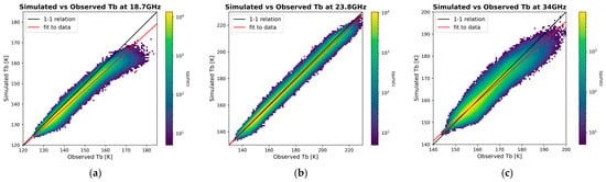
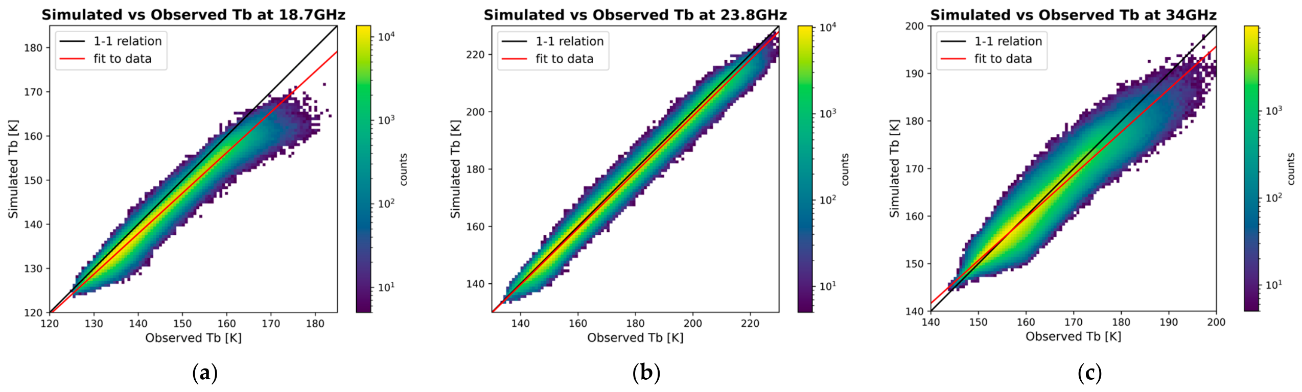
In this section we present the retrieval of a relationship between observed and simulated Tbs for the radiometer AMR-C on board Sentinel-6MF, which will allow for the adjustment of observed Tbs that maximises the performance of the WTC prediction algorithms of this study. The need for this adjustment is due to the fact that correlations between simulated and observed Tbs do not follow a ‘1-1’ relation (see red line in Figure 1). The deviations from a ‘1-1’ relation are due to the limitations in the spatio-temporal representativity of the meteorological models used for the creation of the simulated database, as well as errors from the RTM itself, and potentially instrumental errors and instrument calibration choices [5,10]. As the algorithms developed as part of this study relied on simulated data, the observed Tbs need to be adjusted to account for these discrepancies. Here we detail the selection of collocated observed and simulated Tbs for the AMR-C channels at 18.7 GHz, 23.8 GHz, and 34 GHz, and the methodology developed as part of this study for the retrieval of the optimal correction for the observed Tbs.
Figure 1.
Simulated vs. observed Tbs for the three low-frequency radiometer channels on Sentinel-6MF, at 18.7 GHz (a), 23.8 GHz (b), and 34 GHz (c). The black line corresponds to the ‘1-1’ relationship (i.e., bias of 0 with slope of 1); the red line is the fit to the data.
As detailed in [5], the relationship between observed and simulated Tbs has been defined in the past through an iterative process testing a range of different slopes and biases for each channel, using the results of the linear fit to the data as the starting point. The criteria for the selection of a final set of coefficients included the minimisation of the mean difference of Var(ΔSSH) at crossovers, a mean ΔWTC (difference between predictions and reference) of <1 cm, and a near-Gaussian distribution of ΔWTC. However, the methods used previously are not well documented and were of a more manual approach. Here we have developed a new methodology for the retrieval of the Tb relationship that follows a similar philosophy to what was done previously, but with the aim of creating a reproducible and more autonomous algorithm.
For this we require a large enough dataset of collocated simulated and observed Tbs. We built this database by using the following procedure:
- For each day in the year 2024, and each hour available in the ECMWF analysis (00, 06, 12, 18), we select the track of observed data that is within ±30 min and with latitudes < ±60°.
- We then simulate the Tbs and calculate the WTC for the region (in latitude, longitude) covered by the selected trace for the specified date and hour of the ECMWF data.
- Using the resulting grid of simulated Tbs, we apply linear interpolation to retrieve the corresponding simulated Tbs for each observed position.
Following [5], the resulting dataset is then limited to the following points:
- Validated measurements, based on the calibration and validation process.
- Absolute latitude < 60°, to avoid sea ice in the dataset.
- Absolute ΔTb < 20 K (for all channels), to eliminate points with large differences due to mismatch between the model and observed weather conditions.
- Distance to shoreline > 50 km, to avoid land-contaminated Tbs in coastal regions.
- Absolute difference between operational radiometer TCLWC and TCLWC calculated from ECMWF of <0.1 kg/m2, to ensure cloud conditions between model and observed data are similar.
In the end we have 2.3 × 10⁶ collocated Tbs that can be used to characterise the relationship between simulated and observed Tbs for each channel. In Figure 1 we show the simulated vs. observed Tbs for the channels at 18.7 GHz, 23.8 GHz, and 34 GHz. We see that for 23.8 GHz, the relationship is near linear with a slope of 0.9816, while the other two channels show a stronger deviation from the linear ‘1-1’ relationship with slopes of 0.9177 and 0.9008, for 18.7 GHz and 34 GHz respectively. The observed differences can be attributed to a few known factors, including the lack of spatio-temporal representativity of the ECMWF fields used in our simulations compared to that of the observations. The limitations of the ECMWF representation of cloud coverage and amplitude, and the emissivity models used by the RTM, will propagate through the RTM and affect primarily the 34 GHz and 18.7 GHz channels, respectively. As the impact of the water vapour absorption line is well described by the RTM, and the 23.8 GHz is most sensitive to the water vapour content of the atmosphere and less sensitive to surface conditions and clouds, we see the most agreement between simulated and observed values for this channel.
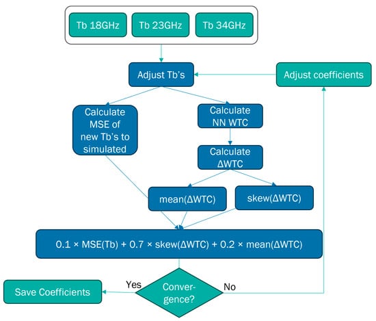
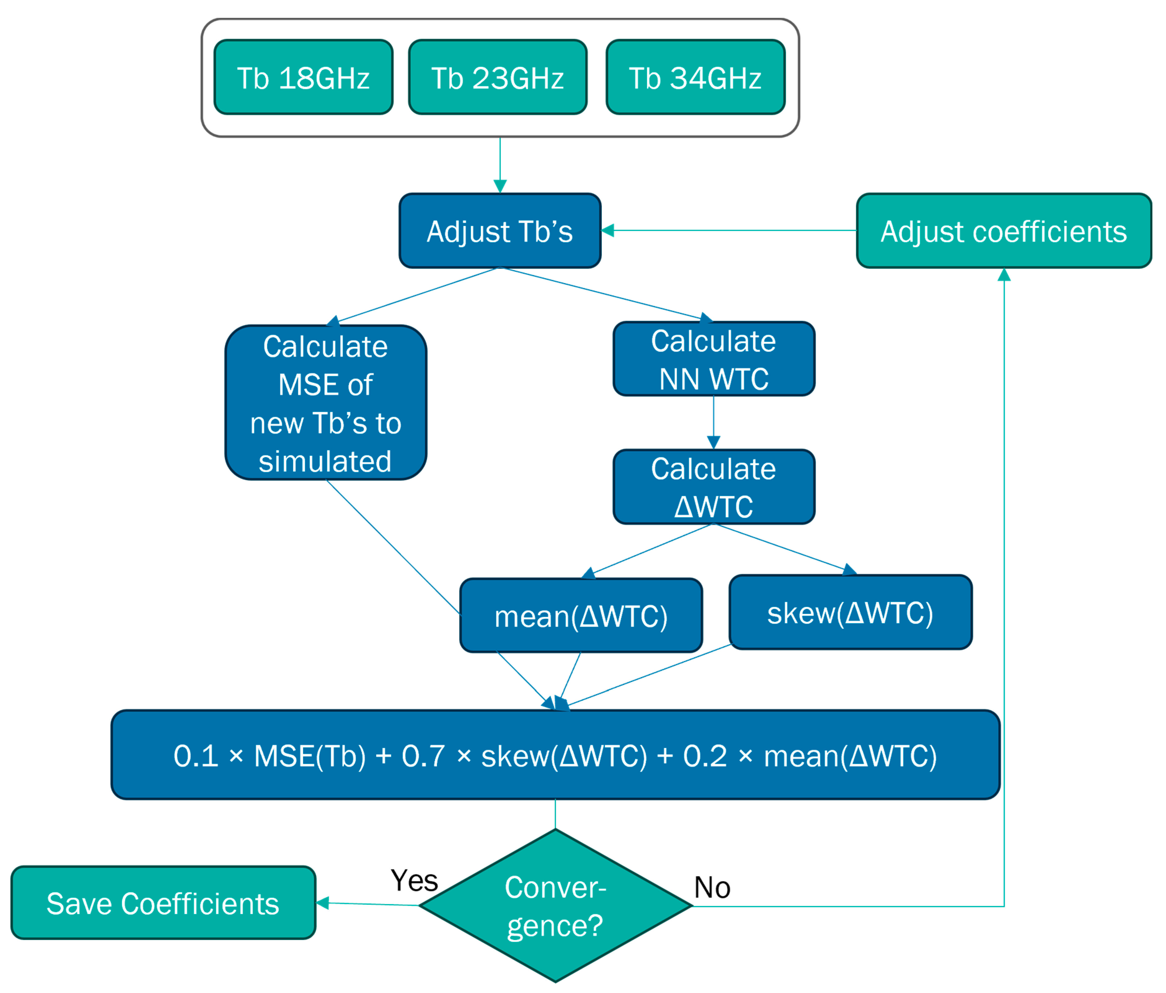
Once the collocated sample has been defined and an initial linear fit to the data has been done, we apply a minimisation algorithm with a custom loss function for the retrieval of the linear transfer function between observed and simulated Tbs. Starting from the linear fit to the data for each channel, the algorithm iteratively adjusts the coefficients of each with the goal of minimising a custom loss function that includes the error on the Tbs (adjusted–simulated), as well as the skewness and mean of the WTC residuals. In Figure 2 we show a schematic of this algorithm. For each iteration the algorithm applies the Tb function with the new coefficients for each channel, calculates the mean square error (MSE) to the corresponding simulated Tbs, applies the NN algorithm on the adjusted Tbs, and calculates the WTC residuals (ΔWTC) and the mean and Kelly skewness () of the ΔWTC distribution. It then calculates the custom loss function:
where , with P10, P50, and P90 corresponding to the 10th, 50th and 90th percentiles. Once the custom loss function remains stable within a tolerance of 10−6, the algorithm stops, and the new coefficients are saved.
Figure 2.
Schematic of the custom loss function method for the retrieval of the best coefficients for the observed Tb adjustment.
The choice of parameters included in the custom loss function is a result of some trial and error. A minimisation of just the mean(ΔWTC) can result in both highly skewed distributions of ΔWTC and coefficients that do not represent the observed range of simulated vs. observed Tbs. A minimisation of only the skewness can result in symmetrical distributions of ΔWTC but with a large mean(ΔWTC) and again with non-realistic results for the Tbs. Furthermore, we tested for different skewness types (modal vs. quantal) and found that our results are improved when using the percentile-based Kelly skewness, which is less sensitive to symmetry in the tails of the distribution than the modal skewness. We have not included the Var(ΔSSH) at crossovers in our calculations as was done by [5], as it would add significant computational time and complexity. However, we did examine the Var(ΔSSH) at crossovers for the resulting coefficients against other solutions tested, to validate the final choice for our algorithm. The final weights selected for the three components of the custom loss function were such as to prioritise a near-Gaussian ΔWTC, reducing the mean(ΔWTC), and retaining adjusted Tbs within the expected parameter range, in decreasing order of weight/importance. To determine the sensitivity of our results to the weights chosen for the custom loss function, we ran a sensitivity test using multiple randomly selected sets of weights (each set adding up to 1) and examined the resulting ΔWTC residual distributions and the difference in Var(ΔSSH) at crossovers for both the NN and LogLin algorithms. We found that the choice of weights for the custom loss function does not greatly affect the resulting ΔWTC and Var(ΔSSH), with all weight sets tested returning distributions of low skewness (<0.03) and mean(ΔWTC) values within 0.2 cm of the results from our original loss function. For comparison, for our original weight selection, we have a skewness of 0 and a mean(ΔWTC) of 0 cm. For the Var(ΔSSH) we find that the results remain within 4% (or 0.006 cm2), for both algorithms. Overall, we find that as long as the three components are included in the function, the relative weights used do not have a strong impact on the final Var(ΔSSH); however, the weights chosen provide the strongest minimisation of the mean and skewness of the ΔWTC distribution.
The resulting Tb transfer functions are given below:
where are the observed, and are the adjusted brightness temperatures at frequency fi of 18.7 GHz, 23.8 GHz, or 34 GHz.
These equations are applied to observed Tbs, and the NN and LogLin algorithms are then applied to the resulting adjusted Tbs.
3. Results
3.1. Performance on Simulated Data
To determine the performance of the two finalised algorithms, we apply each to the Test database created with data from 2024.
Globally, the two algorithms have very similar results, with RMSE of 0.323 cm (CI 95%, 0.320–0.325 cm) and 0.337 cm (CI 95%, 0.332–0.345 cm), for the NN and the LogLin algorithm, respectively (see Table 4). Where CI 95% denotes the 95% confidence interval calculated using a bootstrap analysis.
Table 4.
Global performance metrics from the test database for the two algorithms.
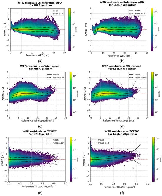
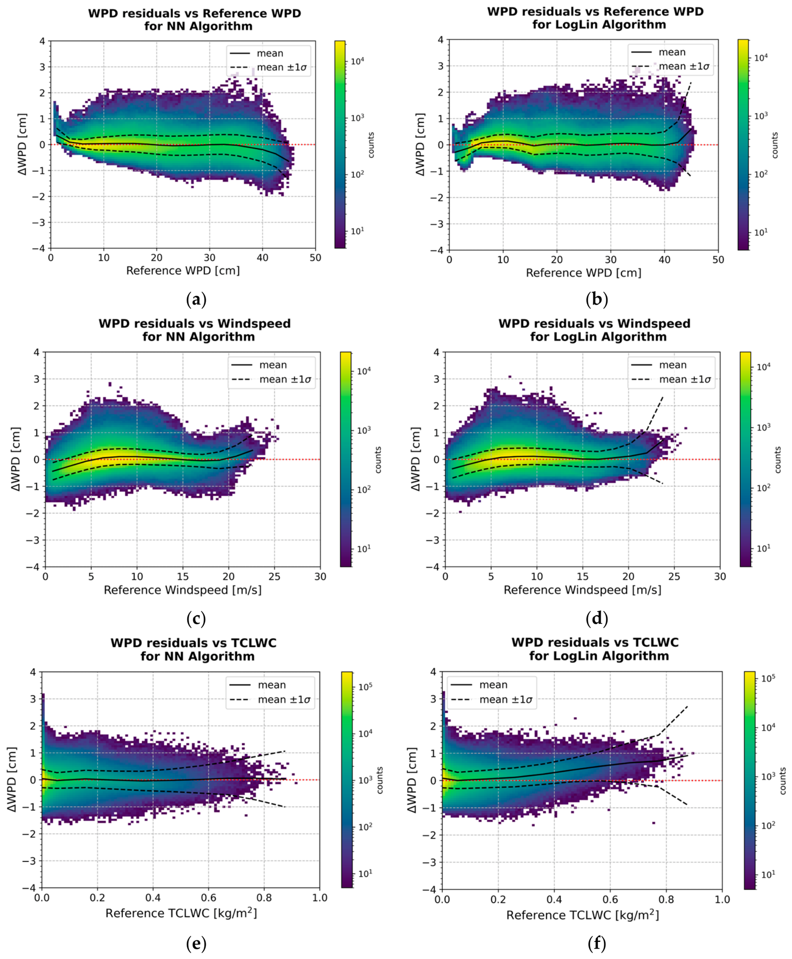
In Figure 3 we show the WPD residuals (ΔWPD) as a function of WPDref, Wref, and TCLWCref. If we focus on the mean and standard deviation of the ΔWPD as a function of WPDref in Figure 3a,b, we see that both algorithms struggle at both low (<5 cm) and high (>35–40 cm) values. Specifically, at WPDref < 5 cm, although the RMSE remains good at values of 0.192 cm (95% CI, 0.190–0.194 cm) and 0.283 cm (95% CI, 0.282–0.285 cm), we see increased biases of 0.104 cm and −0.114 cm for the NN and LogLin algorithms respectively. At WPDref > 40 cm, the RMSE degrades to 0.589 cm (95% CI, 0.585–0.594 cm) and 0.734 cm (95% CI, 0.710–0.757 cm) for the NN and LogLin algorithms respectively. These results are discussed further in Section 4.
Figure 3.
WPD residuals (ΔWPD) as a function of reference WPD (a,b), windspeed (c,d), and TCLWC (e,f). The left column is the NN algorithm; the right column is the LogLin algorithm. In all plots the black solid line corresponds to the mean ΔWPD, with the dashed lines indicating the standard deviation.
As a function of Wref (see Figure 3c,d), again the ΔWPD of the two algorithms show similar behaviour, with both algorithms struggling at low (<5 m/s) and high (>20 m/s) values. At Wref < 5 m/s there are increased biases of −0.188 cm and −0.116 cm, with a small degradation in RMSE with values of 0.383 cm (95% CI, 0.381–0.385 cm) and 0.367 cm (95% CI, 0.364–0.369 cm), for the NN and LogLin algorithms respectively. At Wref > 20 m/s the RMSE significantly degrades to 0.509 cm (95% CI, 0.504–0.514 cm) and 0.810 cm (95% CI, 0.783–0.837 cm).
As a function of TCLWCref (Figure 3e,f), the two algorithms have similar performances for TCLWCref < 0.4 kg/m2, but at TCLWCref > 0.4 kg/m2 the RMSE for both degrades to 0.493 cm (95% CI, 0.488–0.497 cm) and 0.741 cm (95% CI, 0.722–0.760 cm), for the NN and LogLin algorithms respectively.
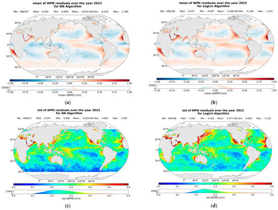
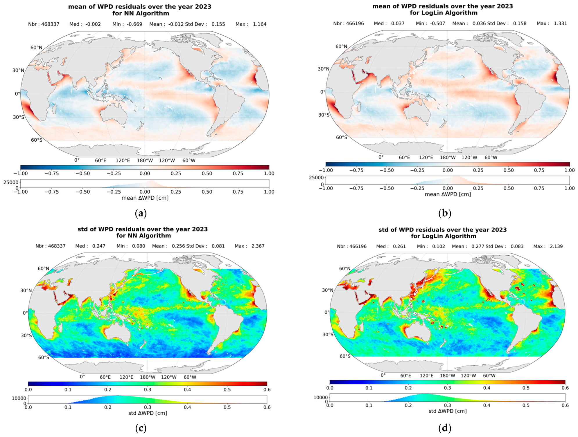
To examine the geographical dependencies in the performance of the algorithms over an independent database from which they were trained, we created maps of the mean and standard deviation of the ΔWPD for the simulated database of 2023. We created maps of the ΔWPD corresponding to each algorithm and calculated the mean and standard deviation of all maps for each pixel. The results are shown in Figure 4. We find that the residuals of both algorithms show similar geographical dependence, with both some latitude dependence and regional dependencies. Similar results were also shown in [6] and attributed to the latitude dependence of sea surface temperature (SST) and upwelling regions. The maps of the standard deviation of the residuals reveal a stronger variability in some regions with larger residuals, as well as regions where there is a large variability in the LogLin residuals that is not seen for the NN.
Figure 4.
Maps of the mean (a,b) and standard deviation (std (c,d)) of the WPD residuals in pixels of 0.25° × 0.25° over the year 2023, for the NN in the left column, and LogLin algorithm in the right column.
3.2. Performance on Observed Data
To examine the performance of our algorithms on observed datasets, we use the Var(ΔSSH). This measure provides an estimate of the overall altimeter system performance, but since the WTC is directly involved in the estimation of SSH, we can quantify the effect that the results from each of our algorithms have when compared to a different solution such as the model (MOD) or operational (OP) WTC. Assuming that there should not be a change in the SSH within a period of 10 days over regions of low oceanic variability, the differences in measured SSH at crossovers of ascending and descending passes of the satellite should be close to zero, and therefore the Var(ΔSSH) within 10 days should be minimal if all corrections were perfectly estimated. In reality, contributions of errors from the different components for the SSH calculation will cause increased values of Var(ΔSSH), with errors of the WTC remaining one of the principal contributors. Therefore, we can determine the relative performance of our two algorithms by comparing to the MOD or OP WTC, and to each other; results that reduce the Var(ΔSSH) can be interpreted as reducing the error on the WTC and therefore improving performance.
We calculate the SSH for each WTC solution examined (NN, LogLin, OP, MOD) by using the uncorrected SSH measurements in the Sentinel-6MF products and applying all the needed corrections, including the WTC. This results in an SSH for each WTC solution calculated in exactly the same way, with the only difference between them being the WTCs used.
In this section we examine both the global performance over open ocean (Section 3.2.1) and within a region of atmospheric upwelling (Section 3.2.2).
3.2.1. Global Performance over Ocean
The observations used for this analysis are limited to the year 2023, validated through the calibration and validation process, with latitudes between 60°N and 60°S, a distance to the shore of >50 km, a bathymetry of <1000 m, and an ocean variability of <0.2 m. We further include a limit on the operational radiometer TCLWC < 1 kg/m2. It should also be noted that we compare to the operational WTC product that is based on the three low-frequency AMR-C channels, and we compare the two algorithms as developed in Section 3.1, i.e., without the inclusion of the liquid water delay that is included in the OP WTC.
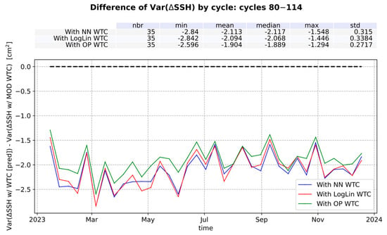
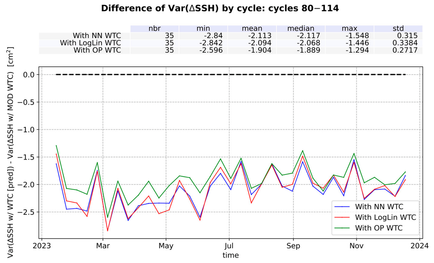
In Figure 5 we show the difference in Var(ΔSSH) between each algorithm and the MOD. The corresponding mean differences are shown above the figure. We find that both solutions provide a significant and very similar improvement, with the mean difference of Var(ΔSSH) = −2.11 (95% CI, −2.22–−2.00) cm2 for the NN, and Var(ΔSSH) = −2.09 (95% CI, −2.21–−1.98) cm2 for the LogLin. This improvement is of a similar scale as what has been shown for other radiometers [5,18], and for comparison, the mean difference of Var(ΔSSH) between the operational product and the model is −1.9 cm2. These results highlight the well-known importance of radiometers for the determination of WTC versus using meteorological models.
Figure 5.
The difference of the temporal evolution between the Var(ΔSSH) from the NN and LogLin algorithms to that from the model (MOD) WTC.
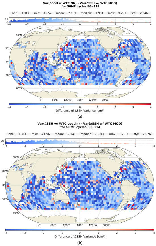
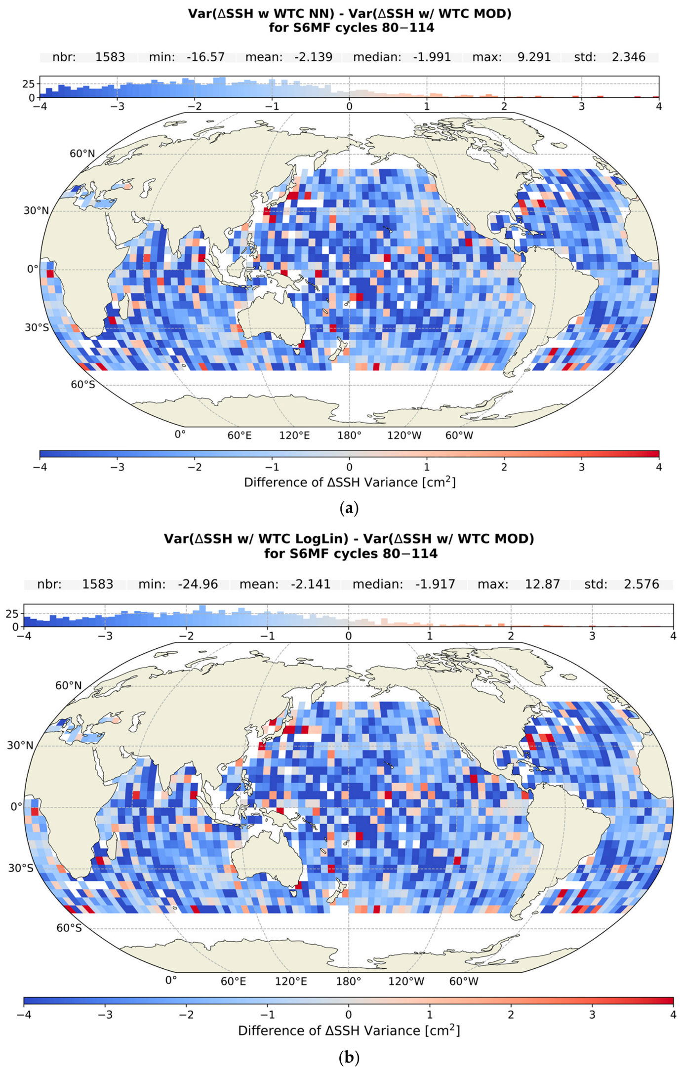
When examining the maps of difference to the model, binned by 4 × 4°, in Figure 6, we can see that both algorithms show significant improvements over most of the ocean, with a mean difference in Var(ΔSSH) of −2.14 cm2 (95% CI, −2.15–−2.12 cm2) for both. Interestingly, we do see that in the regions corresponding to the areas with upwelling, the improvements, although still present, are smaller than the rest of the ocean; we examine this further in Section 3.2.2.
Figure 6.
The differences between maps of Var(ΔSSH) in bins of 4 × 4° between the NN or LogLin and model (MOD) WTC. (a) for the NN; (b) for the LogLin.
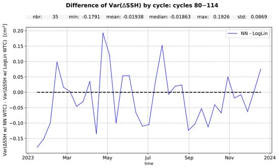
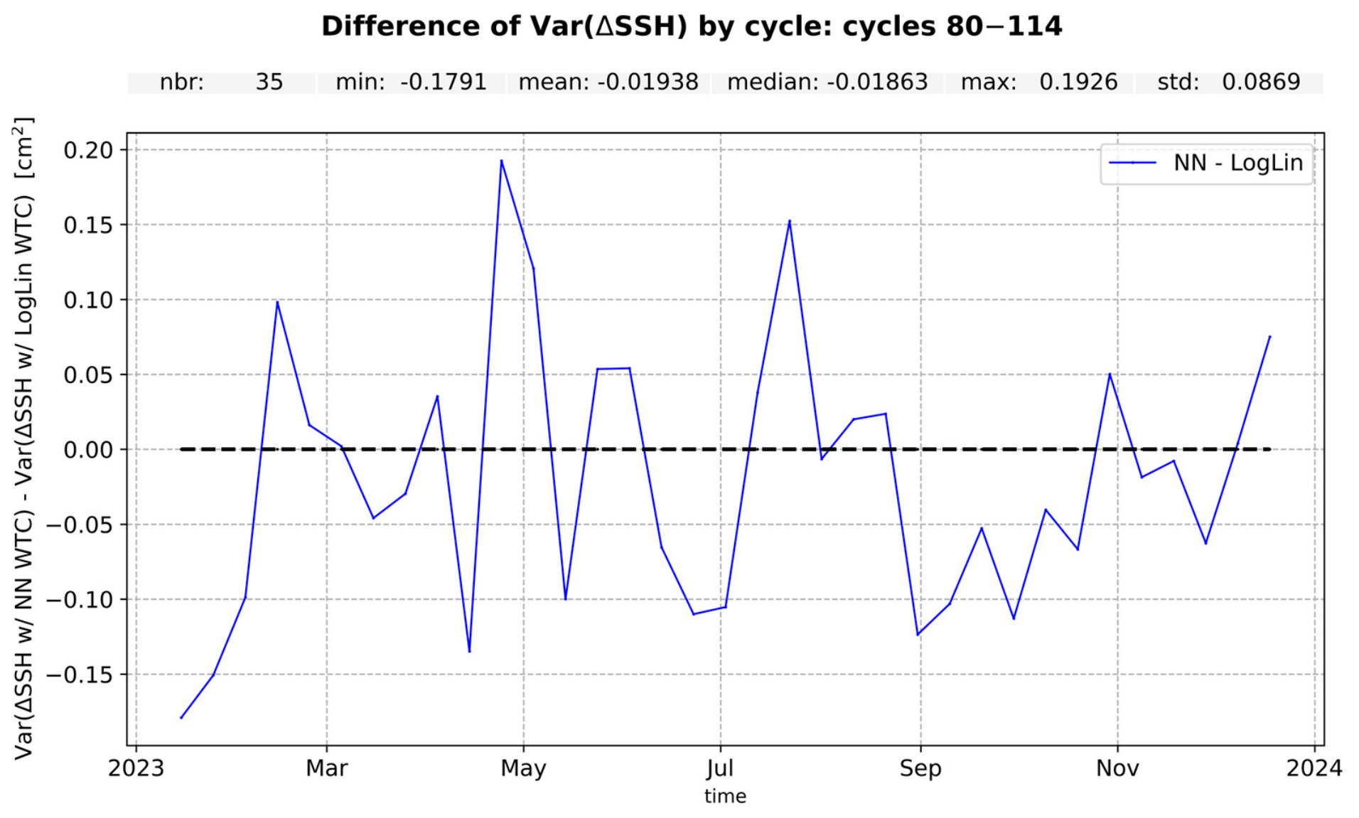
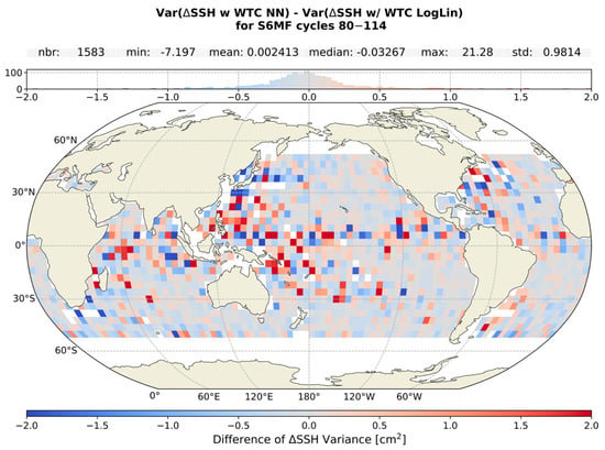
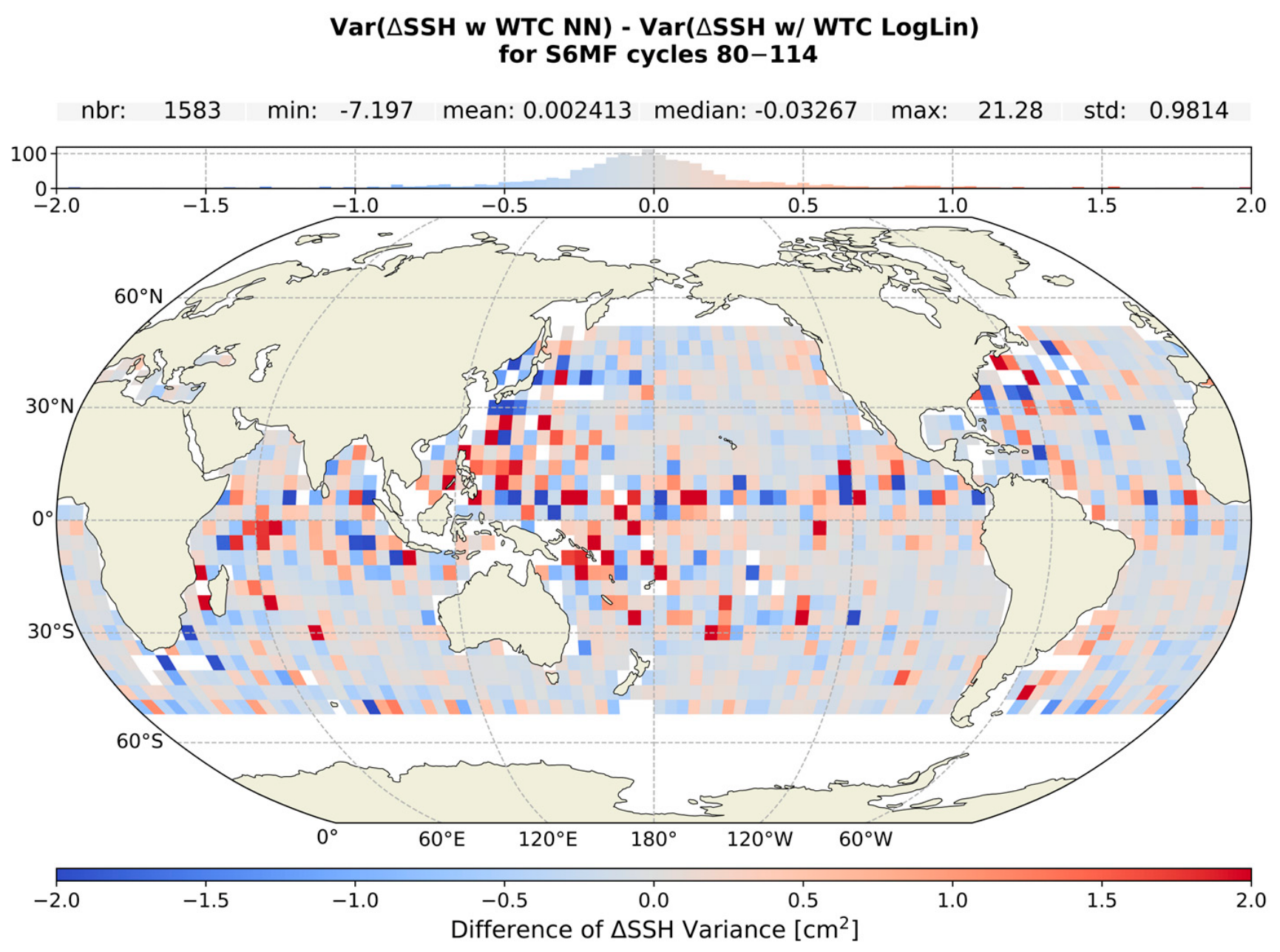
An intercomparison of the two algorithms in Figure 7 and Figure 8 confirms the comparable performance of the two seen when compared to the model, with a difference in Var(ΔSSH) of −0.019 cm2 (95% CI, −0.05–0.01 cm2).
Figure 7.
Intercomparison of the two algorithms with the difference in the temporal evolution of Var(ΔSSH) between the NN and LogLin WTC.
Figure 8.
Map of the intercomparison of the two algorithms. Red indicates that the LogLin is performing better, while blue indicates that the NN is performing better.
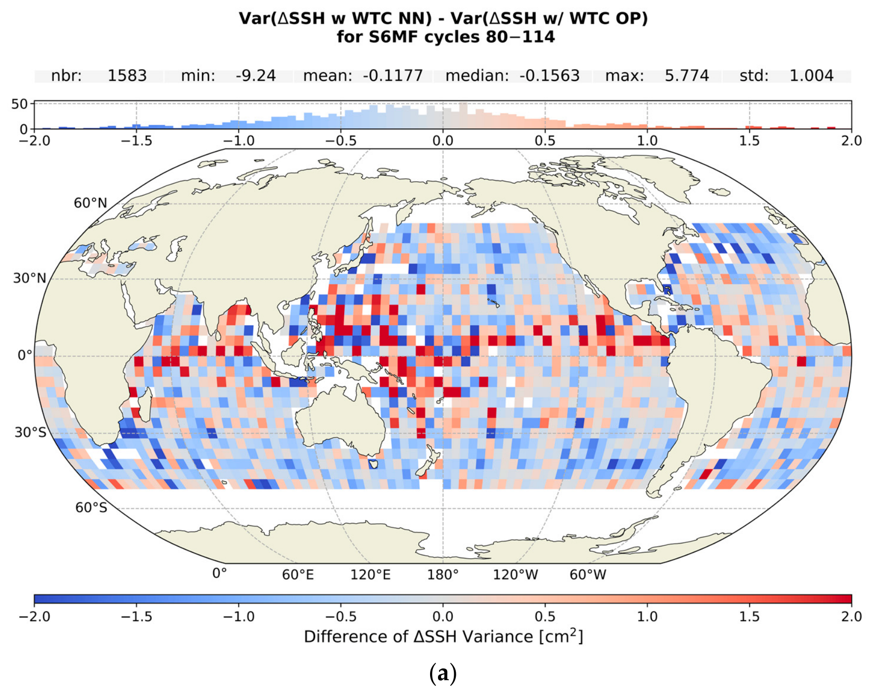
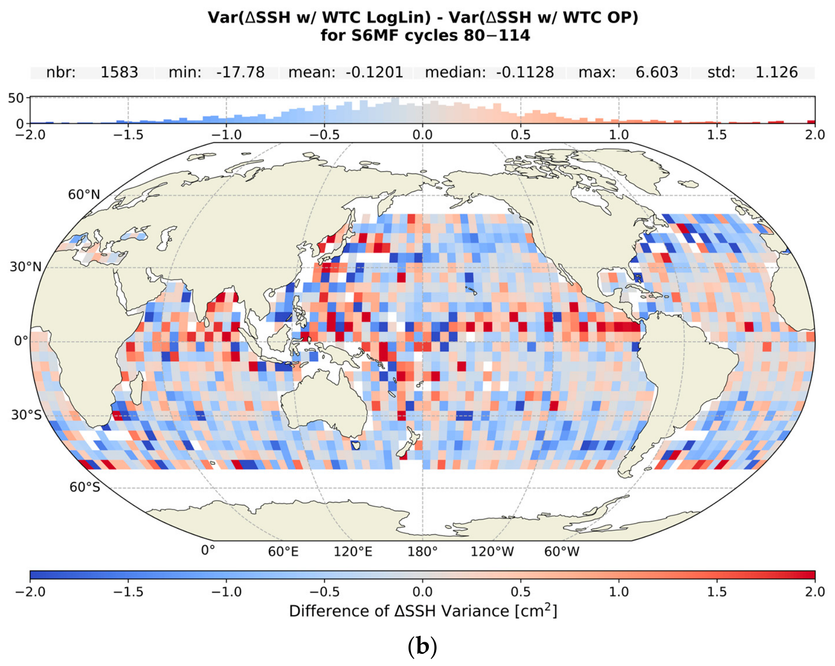
When examining the maps of the Var(ΔSSH) difference, we see that the results are equivalent for the two algorithms, with some bins showing large differences in the equatorial regions where large weather variability is expected to occur. We see similar signatures in the comparisons to the operational product that follow and discuss further in Section 4.
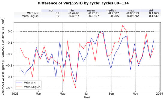
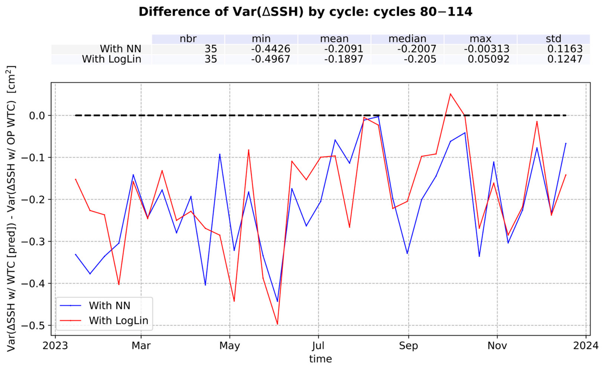
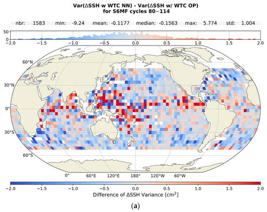
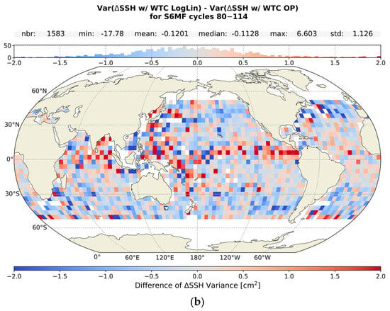
In Figure 9 we show the difference in Var(ΔSSH) between each algorithm and the OP. We find that both our NN and LogLin algorithms perform better than the operational with a mean difference in the Var(ΔSSH) of −0.21 cm2 (95% CI, −0.25–−0.16 cm2) and −0.19 cm2 (95% CI, −0.23–−0.15 cm2), respectively. However, when comparing to the operational results in maps binned by 4 × 4° in Figure 10, we see that although both algorithms mostly perform comparably to or better than the operational results, there are regions of large positive differences (i.e., where our algorithms are performing worse), mostly in the equatorial region.
Figure 9.
The difference in the temporal evolution between the Var(ΔSSH) from the NN and LogLin algorithms and that from the operational (OP) WTC.
Figure 10.
The differences between maps of Var(ΔSSH) in bins of 4 × 4° between the NN (a) or LogLin (b) and operational (OP) WTC.
When binned in lon/lat the resulting mean improvement is in a way normalised for latitude dependence (i.e., more observations at high latitudes than around the equator mean that the large latitude results have more weight in the global average), and as a result the degraded performance in the equatorial region reduces the mean differences to −0.12 cm2 (95% CI, −0.13–−0.11 cm2) for both algorithms compared to the OP. The comparative differences between Figure 9 and Figure 10 highlight that the global mean reduction in the Var(ΔSSH) is dominated by the improvements in regions of larger absolute latitudes, with lower performances around the equator skewing the normalised average to smaller values.
The overall differences in performance observed between our algorithms and the operational product, especially between the LogLin of this study and the OP, could be linked to two factors in the development that differ from those of the OP. For the training database used, operationally, the coefficients of the LogLin algorithm are defined based on a database built from radiosonde data, while for the development of the algorithms in this paper, we used a database built from ECMWF fields. We also apply a Tb adjustment before applying the algorithms, something not done by the operational process; instead, the needed adjustments are absorbed by the calibration of the B coefficients during commissioning (through private communication).
3.2.2. Performance Within a Region of Upwelling
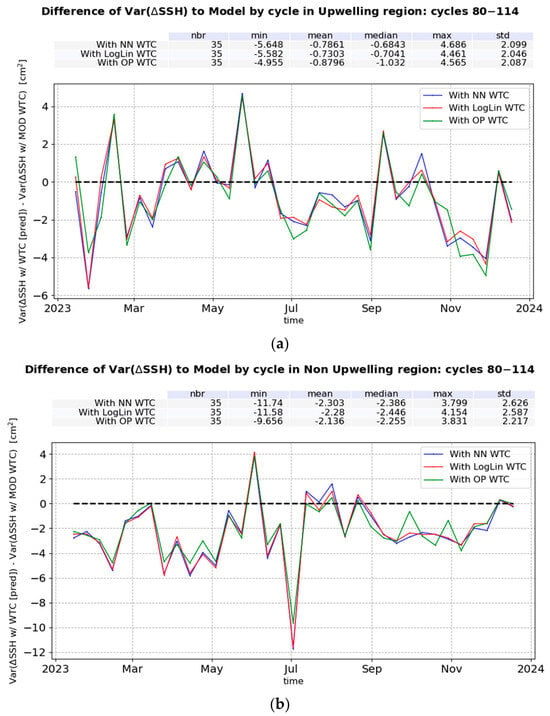
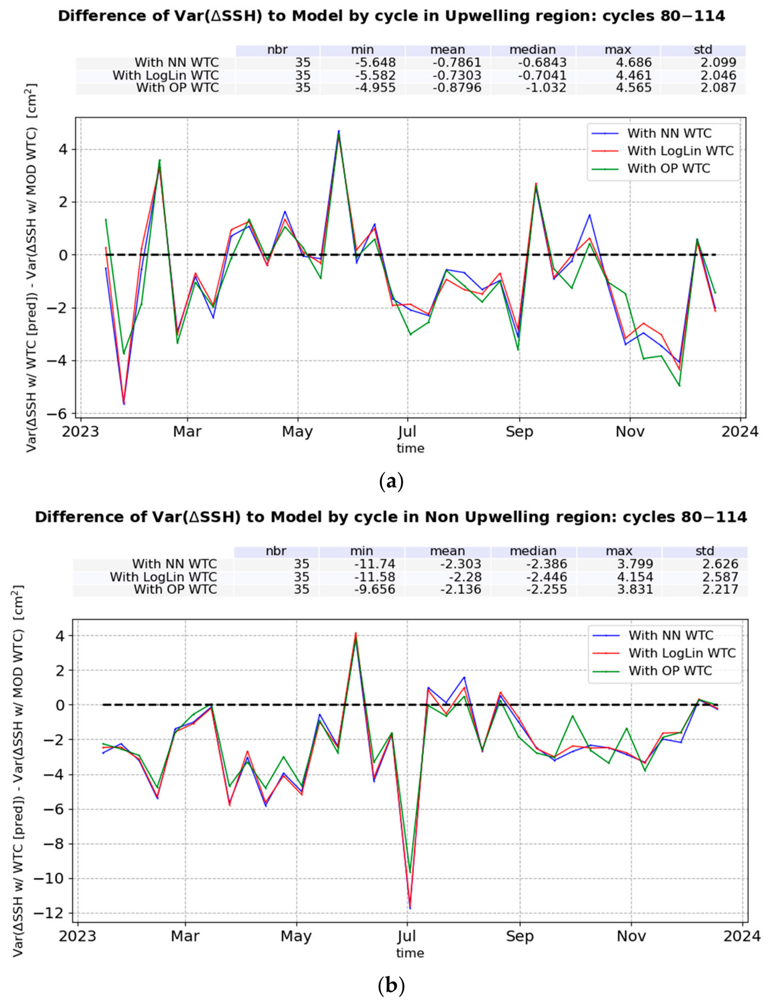
To determine how our algorithms perform within an upwelling region, we examine the Var(ΔSSH) within an upwelling region that remains relatively stable through the year, the region Southwest of Africa. We examine this region’s annual variation and select an area that includes large atmospheric temperature lapse rate (γ800) values for the majority of the year, with coordinates of −25° to −12.5° latitude and 7.5° to 13.5° longitude. As the small size of the region, and therefore the number of points included in the analysis, could significantly affect the results, we also examine a region of similar size with no upwelling, to serve as a comparison. This region is within −25° to −12.5° latitude, and 334 to 340° longitude. In Figure 11a, we show the difference of Var(ΔSSH) to the model as a function of time for the upwelling region, and in Figure 11b, for the non-upwelling region of a similar size.
Figure 11.
The difference in the temporal evolution of Var(ΔSSH) at crossovers between the NN and LogLin algorithms and that from the model WTC, for an Upwelling region (a), and a non-upwelling region of a similar size (b).
We find that in the upwelling region both algorithms examined perform equivalently to each other and the OP WTC and remain better in performance than the MOD WTC, with a difference in Var(ΔSSH) to the model of −0.78 cm2 (95% CI, −1.45–−0.05 cm2) for the NN, and −0.73 cm2 (95% CI, −1.39–−0.02 cm2) for the LogLin. The observed improvements in the upwelling region are significantly smaller compared to those achieved in the non-upwelling region of a similar size, where the difference in Var(ΔSSH) is −2.30 cm2 (95% CI, −3.17–−1.48 cm2) for the NN, and −2.28 cm2 (95% CI, −3.14–−1.47 cm2) for the LogLin. These results suggest a degradation of performance of both algorithms within regions of atmospheric upwelling.
4. Discussion
In this section we discuss the results presented in Section 3, focusing on the limitations found when applying the two algorithms to simulated and observed datasets. Overall, we have found that the two algorithms have similar performance and show similar degradations of performance in certain conditions.
In Section 3.1 we presented the results from applying the two algorithms on simulated datasets. We examined the residuals as a function of WPDref, Wref, and TCLWCref, and found that both algorithms degrade in performance for low and high WPDref (at <5 cm and >40 cm), low and high Wref (<5 m/s and >20 m/s), and for TCLWCref > 0.4 kg/m2. Indeed, for most of these value ranges we have a significantly smaller percentage of the data available for both training and test databases, with only 6.2% of data with WPDref < 5 cm, 0.97% of data with WPDref > 40 cm, 0.25% with Wref > 20 m/s, and 1.1% with TCLWCref > 0.4 kg/m2. Interestingly, for Wref < 5 m/s there is a much better fraction of data at 23.4%, suggesting that the degradation observed for low wind speeds is not due to low representativity in the training database but rather due to limitations in the algorithms and/or their inputs. The stronger degradation observed for the LogLin algorithm at large WPDref and TCLWCref values, compared to the NN, is most likely due to the difference in nature of the two algorithms, with the LogLin built on linear equations that are more sensitive to extreme values and can easily surpass the representative parameter range of the training database, while the NN uses non-linear equations and is more likely to stay within the parameter range it was trained in.
In Section 3.2.1 we presented the results when applying the two algorithms to observed data for the year 2023 and examined the relative performance of both algorithms using the difference in the Var(ΔSSH) to each other, to the operational, and to the model. We have found that when applied to observations, the two algorithms show overall very similar performance to each other and similar to, and often better than, the operational product. However, we note strong variability around the equatorial zone extending to ±20° latitude, where we see many strong positive and negative differences when comparing the two algorithms to the operational product (Figure 10) and in the intercomparison of the two algorithms (Figure 8). Similar results were also seen in the previous analysis of [7] (see their Figure 8), although not specifically discussed. There are a number of possible contributors to this observed behaviour around the equatorial zone. Regions of small absolute latitudes have the largest absolute values of WTC and are also regions of high variability both in meteorological conditions and in the resulting WTC. These regions also have overall smaller numbers of observations within a specified bin than a similar bin at larger absolute latitudes. Therefore, we could expect that in bins with smaller number statistics located in regions of large meteorological variability, it is more likely that the presence of significant outliers can easily skew the statistics. To explore this hypothesis, we examine the counts of each bin, and we examine maps of Rainfall rate and TCLWC from the Global Precipitation Measurement (GPM) Microwave Imager (GMI), a radiometer focused on the observation and measurement of precipitation. We find that the counts per bin for our maps range from 10 to 340, with the majority of bins within latitudes of ±20° having a count between 60 and 150. However, we do find that for the regions where the large Var(ΔSSH) differences have been noted, bin counts are reduced to <60. If we look at the statistics within the area examined, 58 bins have an absolute difference of Var(ΔSSH) > 2 cm2; of these bins, 34 (58.6%) have less than 60 counts.
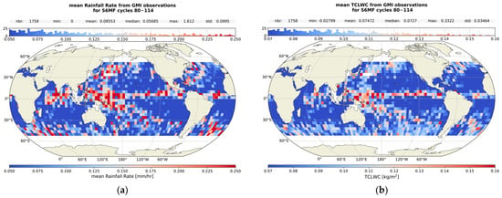
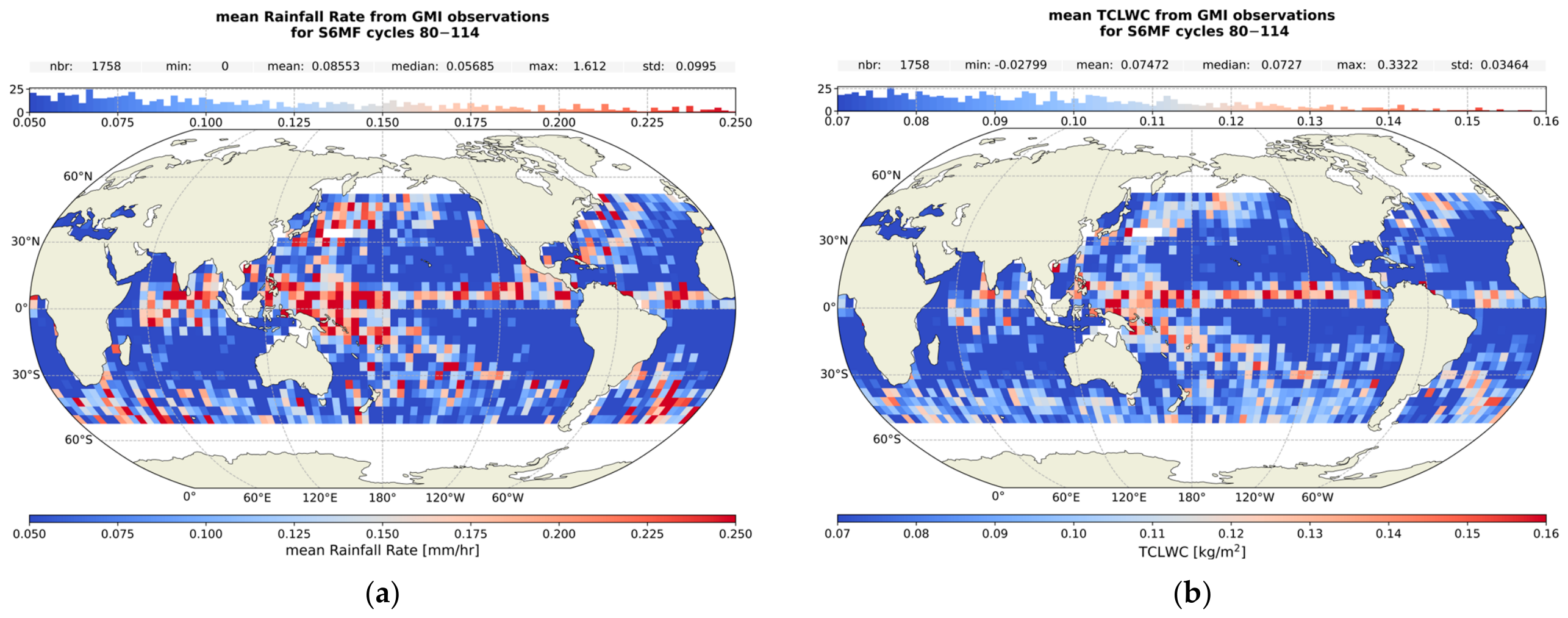
To confirm whether the data in the equatorial region where we see such large differences correspond to regions of significant weather variability that can cause outliers to dominate the resulting statistics (despite the validity selection applied for this analysis), we collocated data from GMI with Sentinel-6MF observations with a Δt < ±120 min. This results in 13.7% of Sentinel-6MF ocean observations with collocated measurements from the GMI. We create 4 × 4° binned averaged maps, shown in Figure 12, applying the same selection as the Var(ΔSSH) analysis. Although these maps are not directly equivalent to the ones made using the Sentinel-6MF observations, they can indicate typical meteorology in the regions that would be affecting the radiometer measurements and the Var(ΔSSH). Also note that although we have selected data where the operational Sentinel-6MF TCLWC product does not exceed 1 kg/m2, we do not limit the TCLWC of the GMI products.
Figure 12.
Maps of the mean Rainfall Rate (a) and TCLWC (b) from GMI collocated to the Sentinel-6 observations, in bins of 4 × 4°.
For both maps we see a concentration of strong rainfall and larger values of TCLWC in the equatorial region, in agreement with the locations of large observed differences in Var(ΔSSH), with some additional locations near Japan, India, and North-East America. Using the above maps we can determine that for the 58 bins within ±20° of the equator with an absolute difference of Var(ΔSSH) > 2 cm2, there is evidence of rain in 48 bins (83%), with a median bin count of 57. However, not all regions of rainfall and large TCLWC have equivalent large differences in performance to the operational. Overall, based on the above results, we can conclude that the large differences observed are at least partially due to the more variable conditions present that can significantly skew the distribution of a bin that is not largely populated. These regions have a significant role in the degradation of performance when comparing the two algorithms and highlight the limitations of the two algorithms in situations of rainfall and significant cloud coverage.
In Section 3.2.2 we examined the performance of the two algorithms within a region of upwelling and found a degradation in performance compared to a non-upwelling region of a similar size. The observed degradation is not likely due to the small number of crossovers, as the non-upwelling region of similar size does not show such degradation. In addition, in Figure 12 there are very low values in Rainfall Rate and TCLWC in the upwelling regions, making the observed degradation in performance unlikely to be linked to these conditions. The observed degradation in performance within upwelling regions can be linked to a lack of information carried by the input Tbs themselves on the behaviour of the atmospheric temperature gradient or the temperature profile, therefore in regions where the profile behaves differently to the norm, such as these regions of upwelling, the algorithms are not able to best constrain the WTC without the inclusion of additional inputs such as the sea surface temperature (SST) and the γ800 itself (see e.g., [6,19]), although there is an argument by [20] that the addition of SST can suffice if using dynamic maps.
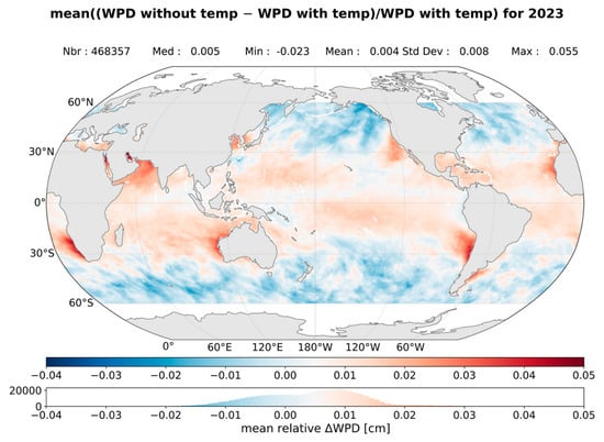
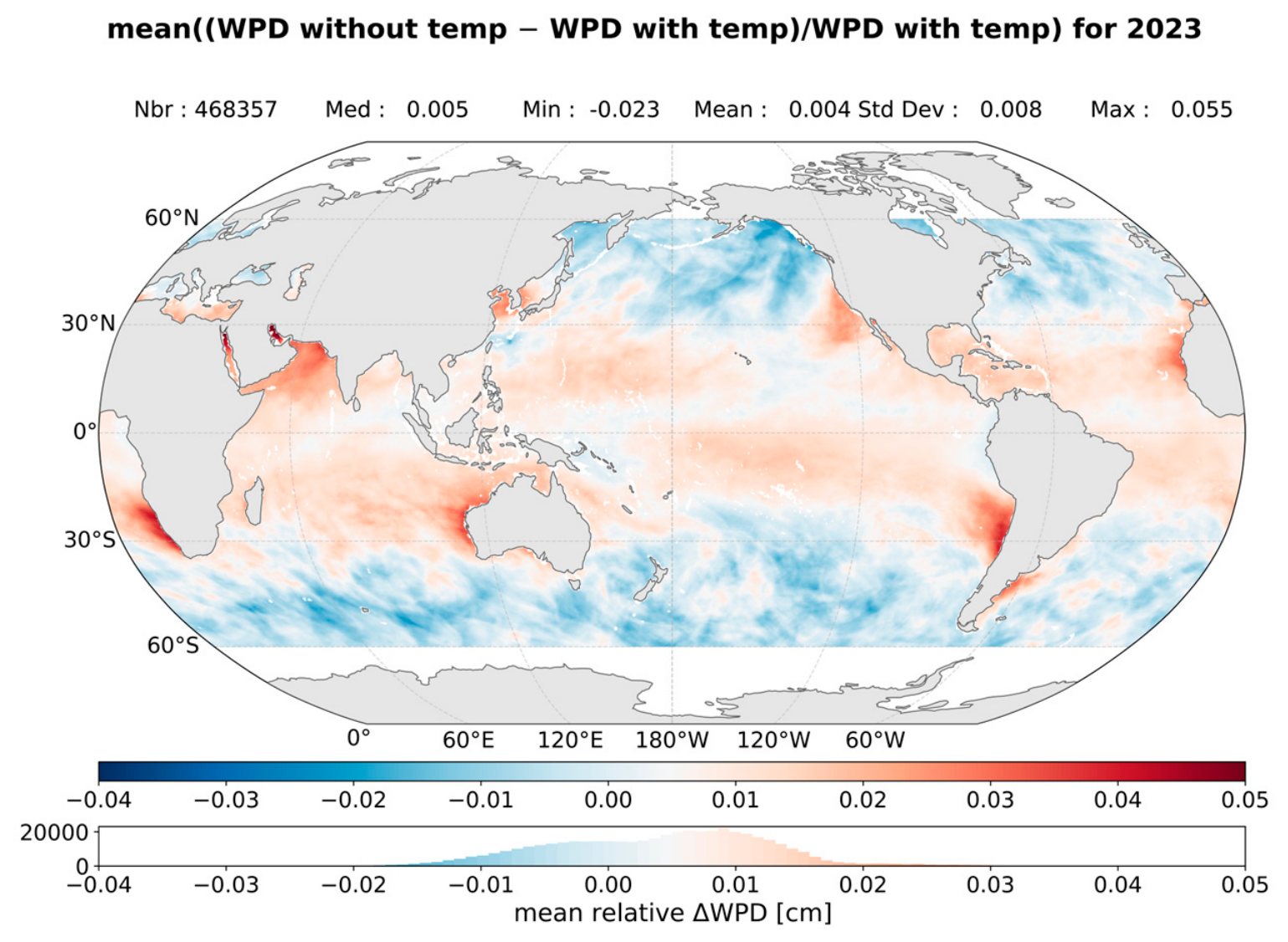
We can demonstrate this lack of information carried by the inputs to the algorithms by comparing the WPD calculated using the theoretical Equation (2), which includes both the water vapour and the temperature profiles, to that calculated approximately using only the total column water vapour (TCWV) with the empirical equation from [21], and the updated coefficients from [22].
In Figure 13, we show the averaged relative difference between a WPD calculated from the integrated TCWV (from ECMWF), and the WPD as we have calculated it for our database used for development using Equation (2). We used one map per month of 2023 to calculate the average over the year. We see that a lack of temperature information when estimating the WTC, has a clear impact on the results, with the largest relative differences in regions of upwelling; however, these differences show an overall structure that suggests a general impact on WTC estimates not limited to upwelling regions. Therefore, we may conclude that the limitations faced by both the new and operational algorithms discussed above could be at least partially explained by a lack of key information in the inputs to the algorithms. It remains an open question whether the needed additional information could come from additional constraints on the SST, the atmospheric temperature lapse rate that carries information on the profile of the atmospheric temperature, or additional radiometer channels probing different levels of the troposphere.
Figure 13.
Map of the mean relative difference between a WPD estimated using only the TCWV and that using the complete Equation (2). This map shows how a lack of information on the atmospheric temperature profile directly impacts the WPD estimations, with the upwelling regions showing the largest rel. differences.
5. Conclusions
The aim of this study was to develop and compare the mathematical aspects of the two main algorithms used operationally by altimetric missions for the estimation of the WTC from the radiometer brightness temperatures, with the purpose of characterising how the differences in the approaches of the two algorithms affect the resulting WTC products, their performance and their limitations. The development was done using the same simulated data for Copernicus Sentinel-6MF, and comparison of the algorithms is done using both simulated and observed Copernicus Sentinel-6MF data, allowing us to characterize the differences due to the algorithms themselves.
Specifically, we have developed an altered version of the CLS NN (developed for two-channels radiometers) that normally takes as input the σ0 of the altimeter measurement and the two brightness temperatures from the 23.8 GHz and 36.5 GHz channels on board missions such as Sentinel-3, and instead we use the three radiometer channels available on Copernicus Sentinel-6MF, therefore including the 18.7 GHz brightness temperature in place of σ0, and the 34 GHz channel in place of 36.5 GHz (see Section 2.3). We developed the LogLin algorithm used by JPL following the relevant documentation (see Section 2.4); excluding, however, the liquid component in order to compare like-to-like with the NN. Both algorithms were then trained/developed using the same set of training data of simulated Tbs, and reference WTC values based on ECMWF fields for the year 2024 (see Section 2.1).
As part of this study, we also developed a new methodology to determine the Tb Transfer Function (see Section 2.5). This performs a necessary adjustment of the observed Tbs to the statistical plane of the simulated Tbs on which the algorithms were trained.
When applied to simulated datasets, the NN shows somewhat better global performance than the LogLin, with an RMSE of 0.323 cm (CI 95%, 0.320–0.325 cm) and 0.337 cm (CI 95%, 0.332–0.345 cm) for the NN and LogLin algorithms respectively. We examined the performance metrics of the algorithms as a function of WTC, W and TCLWC, and found that although the NN provides somewhat better results throughout, both algorithms degrade in performance significantly at WTC values of >−5 cm and <−40 cm, W < 5 m/s and >20 m/s, and TCLWC > 0.4 kg/m2. The residuals of both algorithms show similar geographical dependence, with both some latitude and regional dependencies, similar to what has been noted in previous studies and attributed to the latitude dependence of sea surface temperature and to upwelling regions [6,19]. The maps of the standard deviation of the residuals reveal a stronger variability coinciding with regions of large residuals; we also note more regions of large variability in the residuals of the LogLin algorithm than seen for the NN (see Section 3.1).
When applied to the Copernicus Sentinel-6MF AMR-C observations for the year 2023, we find that both perform to an equivalent level; both improve global performance to the operational WTC product, with a mean difference in Var(ΔSSH) of −0.21 cm2 (95% CI, −0.25–−0.16 cm2) and −0.19 cm2 (95% CI, −0.23–−0.15 cm2), for the NN and LogLin respectively. Both provide a significant improvement compared to the ECMWF-derived WTC that can be expected from MWR, with a difference in Var(ΔSSH) of −2.14 cm2 (95% CI, −2.15–−2.12 cm2) for both. However, in the equatorial regions where the largest WTC values and large weather variability occur, there is a strong variability in the observed relative performance of the two algorithms to that of the operational (see Section 3.2.1). When we examine the performance within an atmospheric upwelling region the performance of the algorithms degrades significantly when compared to a non-upwelling region of a similar size, with both algorithms and the operational WTC product degrading in a similar way, where the difference in Var(ΔSSH) compared to the model WTC is reduced to −0.78 cm2 (95% CI, −1.45–−0.05 cm2) in comparison to −2.30 cm2 (95% CI, −3.17–−1.48 cm2) in an non upwelling region for the NN, and −0.73 cm2 (95% CI, −1.39–−0.02 cm2) instead of −2.28 cm2 (95% CI, −3.14–−1.47 cm2) for the LogLin, a similar degradation is present for the operational WTC product (see Section 3.2.2).
When bringing together all the results presented in this study, we have found that despite the very different approaches of the two algorithms, when trained and applied on the same databases, both the overall performance and the limitations in performance faced by each are comparable. The degradation in performance observed for both algorithms at the two extremes of the WTC range, at large windspeeds and large TCLWC, is likely at least partially due to lack of representativeness in the training database, as discussed in Section 4. However, in the case of low windspeeds, the degradation observed is not due to a lack of data, and as both algorithms are showing a very similar degradation despite very different approaches, it is most likely that the limitations in performance are due to lack of information carried by the inputs themselves. The degradation in performance observed around the equatorial region, when looking at the Var(ΔSSH), is most likely due to the presence of rain not necessarily caught by the quality flags, affecting the WTC estimates. Finally, in upwelling regions we observe both large WTC residuals and a degradation in performance when looking at the Var(ΔSSH) from observations, again for both algorithms. As these regions do not show evidence of the presence of rain or significant TCLWC, and we have removed the possibility that it is caused by lower-number statistics by comparing to a non-upwelling region of a similar size, the degradation in performance is most likely due to limitations of the inputs themselves (see also [6,7]). This is likely because the three brightness temperatures used mostly probe lower levels of the troposphere and therefore lack information on the behaviour of the atmospheric temperature profile, which will have an impact on WTC estimates. This has previously been somewhat remedied by including additional temperature information from climatology maps of the SST and γ800, such as in the 5P NN [6]. However, at the time of publication, those solutions remain limited by the use of static climatology maps. With the emergence of modern altimetry missions that carry higher-frequency MWR channels, which probe different levels of the troposphere than the lower-frequency ones, it is possible to add the needed temperature profile information by including these high frequencies into our WTC prediction algorithms. An investigation into the possible improvements that could be achieved for WTC algorithms that include the high frequencies available in modern radiometers would be beneficial, both for the better exploitation of current missions such as Copernicus Sentinel-6, and for the preparation of future missions such as Sentinel-3NGT. For missions that are limited to only the lower frequency channels, further investigation is warranted into how best to include the needed additional information for the atmospheric temperature profile, by examining improvements that can be achieved by using more dynamic SST and γ800 maps in place of the currently used static climatology maps (see [20]). Furthermore, improvements on the current three input NN WTC algorithms could be achieved through new deep-learning approaches and enhanced mathematical formulations, an exploration of which could allow for strengthening algorithm robustness, especially in low and high WTC and W conditions.
Overall, we find that despite their different approaches, when the NN and the class-based LogLin algorithms are developed in the same way, on the same database, they exhibit very similar performances and face similar limitations likely linked to the limitations in the inputs used.
Author Contributions
Methodology, software, data curation, formal analysis, visualization, writing—original draft preparation, F.S.; Conceptualization, L.A., L.H. and B.P.; supervision and writing—review and editing, L.A., L.H., B.P., X.B., M.-L.F. and N.P.; funding acquisition, L.H., P.G., N.P. and G.D. All authors have read and agreed to the published version of the manuscript.
Funding
This study was funded by the French space agency (Centre National d’Etudes Spatiales) in the framework of their contribution to the Copernicus Sentinel-3 New Generation Topography mission, the SALP project (260324), and with internal funding from CLS.
Data Availability Statement
The altimetry data for Sentinel-6MF was downloaded from Aviso+ via http://www.aviso.altimetry.fr (accessed 29 October 2026). ECMWF fields were downloaded from the Meteorological Archival and Retrieval System (MARS). The WTCs produced by the two algorithms presented in this study and used in our analysis are available upon request to the authors.
Acknowledgments
The authors would like to thank Bastien Courcol, Emeline Cadier, and their colleagues for building the Sentinel-6MF nadir dataset available at CLS and the provision of the validity flag from cal/val activities to discard all questionable measurements. The authors would like to thank Shannon Brown for clarifications provided pertaining to the operational JPL WTC algorithm. Finally, the authors would like to thank the reviewers for their constructive comments during the publication process.
Conflicts of Interest
Authors Flora Stanley, Laiba Amarouche and Bruno Picard were employed by the company Collecte Localisation Satellites and Fluctus. The remaining authors declare that the research was conducted in the absence of any commercial or financial relationships that could be construed as a potential conflict of interest.
Abbreviations
The following abbreviations are used in this manuscript:
| CLS | Collecte Localisation Satellites |
| JPL | NASA Jet Propulsion Laboratory |
| ECMWF | European Centre for Medium-Range Weather Forecasts |
| MWR | Microwave Radiometer |
| AMR-C | Advanced Microwave Radiometer-C |
| MSL | Mean Sea Level |
| SSH | Sea Surface Height |
| SST | Sea Surface Temperature |
| WPD | Wet Path Delay |
| WTC | Wet Tropospheric Correction |
| TCWV | Total Cloud Water Vapor |
| RTM | Radiative Transfer Model |
| RTTOV | Radiative Transfer for TOVS |
| GMI | GPM Microwave Imager |
| SSM/I | Special Sensor Microwave-Imager |
| NN | Neural Network |
| LogLin | Log-Linear |
| RMSE | Root Mean Square Error |
References
- Fernandes, M.J.; Lázaro, C.; Vieira, T. On the role of the troposphere in satellite altimetry. Remote Sens. Environ. 2021, 252, 112149. [Google Scholar] [CrossRef] [Scilit]
- Chelton, D.B.; Ries, J.C.; Haines, B.J.; Fu, L.-L.; Callahan, P.S. Satellite altimetry. In Satellite Altimetry and Earth Sciences: A Handbook of Techniques and Applications; Fu, L.L., Cazenave, A., Eds.; Academic Press: Cambridge, MA, USA, 2001; pp. 1–131. [Google Scholar]
- Keihm, S.J.; Janssen, M.A.; Ruf, C.S. TOPEX/POSEIDON microwave radiometer (TMR): III. Wet troposphere range correction algorithm and pre-launch error budget. IEEE Trans. Geosci. Remote Sens. 1995, 33, 147–161. [Google Scholar] [CrossRef] [Scilit]
- Obligis, E.; Eymard, L.; Tran, N.; Labroue, S.; Femenias, P. First three years of the microwave radiometer aboard Envisat: In-flight calibration, processing, and validation of the geophysical products. J. Atmos. Ocean. Technol. 2006, 23, 802–814. [Google Scholar] [CrossRef] [Scilit]
- Frery, M.-L.; Siméon, M.; Christophe, G.; Féménias, P.; Borde, B.; Houpert, A.; Garcia, A.O. Sentinel-3 microwave radiometers: Instrument description, calibration and geophysical products performances. Remote Sens. 2020, 12, 2590. [Google Scholar] [CrossRef] [Scilit]
- Obligis, E.; Rahmani, A.; Eymard, L.; Labroue, S.; Bronner, E. An improved retrieval algorithm for water vapor retrieval: Application to the Envisat microwave radiometer. IEEE Trans. Geosci. Remote Sens. 2009, 47, 3057–3064. [Google Scholar] [CrossRef] [Scilit]
- Thao, S.; Eymard, L.; Obligis, E.; Picard, B. Comparison of regression algorithms for the retrieval of the wet tropospheric path. IEEE J. Sel. Top. Appl. Earth Obs. Remote Sens. 2015, 8, 4302–4314. [Google Scholar] [CrossRef] [Scilit]
- Guissard, A.; Sobieski, P. An approximate model for the microwave brightness temperature of the sea. Int. J. Remote Sens. 1987, 8, 1606–1627. [Google Scholar] [CrossRef] [Scilit]
- Boukabara, S.A.; Eymard, L.; Guillou, C.; Lemaire, D.; Sobieski, P.; Guissard, A. Development of a modified two-scale electromagnetic model simulating both active and passive microwave measurements: Comparison to data remotely sensed over the ocean. Radio Sci. 2002, 37, 1063. [Google Scholar] [CrossRef] [Scilit]
- Picard, B.; Frery, M.-L.; Obligis, E.; Eymard, L.; Steunou, N.; Picot, N. SARAL/AltiKa Wet Tropospheric Correction: In-Flight Calibration, Retrieval Strategies and Performances. Mar. Geod. 2015, 38, 277–296. [Google Scholar] [CrossRef] [Scilit]
- Islam, T. Sentinel 6 Project: Advanced Microwave Radiometer Level 2 Algorithm Theoretical Basis Document, JPL D-103429. Available online: https://user.eumetsat.int/s3/eup-strapi-media/D_103429_S6_AMR_ATBD_20200719_w_sig_16fac58a45.pdf (accessed on 29 October 2026).
- Saunders, R.; Hocking, J.; Turner, E.; Rayer, P.; Rundle, D.; Brunel, P.; Vidot, J.; Roquet, P.; Matricardi, M.; Geer, A. An update on the RTTOV fast radiative transfer model (currently at version 12). Geosci. Model Dev. 2018, 11, 2717–2737. [Google Scholar] [CrossRef] [Scilit]
- Bean, B.R.; Dutton, E.J. Radio Meteorology; U.S. NBS Monograph: Washington, DC, USA, 1966; Volume 92. [Google Scholar]
- CLS-DOS-NT-09-119, 2011, Surface Topography Mission (STM) SRAL/MWR L2 Algorithms Definition, Accuracy and Specification [SD-03][SD-07]. Available online: https://user.eumetsat.int/s3/eup-strapi-media/pdf_s3_alt_level_2_adas_23dcc1ef2d.pdf (accessed on 29 October 2026).
- Saastamoinen, J. Atmospheric correction for the troposphere and stratosphere in radio ranging satellites. Use Artif. Satell. Geod. 1972, 15, 247–251. [Google Scholar] [CrossRef] [Scilit]
- Davis, J.L.; Herring, T.A.; Shapiro, I.I.; Rogers, A.E.E.; Elgered, G. Geodesy by radio interferometry: Effects of atmospheric modeling errors on estimates of baseline length. Radio Sci. 1985, 20, 1593–1607. [Google Scholar] [CrossRef] [Scilit]
- Donlon, J.C.; Cullen, R.; Giulicchi, L.; Vuilleumier, P.; Richard Francis, C.; Kuschnerus, M.; Simpson, W.; Bouridah, A.; Caleno, M.; Bertoni, R.; et al. The Copernicus Sentinel-6 mission: Enhanced continuity of satellite sea level measurements from space. Remote Sens. Environ. 2021, 258, 112395. [Google Scholar] [CrossRef] [Scilit]
- Legeais, J.-F.; Ablain, M.; Thao, S. Evaluation of wet troposphere path delays from atmospheric reanalyses and radiometers and their impact on the altimeter sea level. Ocean Sci. 2014, 10, 893–905. [Google Scholar] [CrossRef] [Scilit]
- Sun, J. Effects of vertical distribution of water vapor and temperature on total column water vapor retrieval error. J. Geophys. Res. 1993, 98, 7069–7079. [Google Scholar] [CrossRef] [Scilit]
- Vieira, T.; Fernandes, M.J.; Lázaro, C. An enhanced retrieval of the wet tropospheric correction for Sentinel-3 using dynamic inputs from ERA5. J. Geod. 2022, 96, 28. [Google Scholar] [CrossRef] [Scilit]
- Keihm, S.J.; Zlotnicki, V.; Ruf, C.S. TOPEX microwave radiometer performance evaluation. IEEE Trans. Geosci. Remote Sens. 2000, 38, 1379–1386. [Google Scholar] [CrossRef] [Scilit]
- Barnoud, A.; Picard, B.; Meyssignac, B.; Marti, F.; Ablain, M.; Roca, R. Reducing the uncertainty in the satellite altimetry estimates of global mean sea level trends using highly stable water vapor climate data records. J. Geophys. Res. Oceans 2023, 128, e2022JC019378. [Google Scholar] [CrossRef] [Scilit]

Disclaimer/Publisher’s Note: The statements, opinions and data contained in all publications are solely those of the individual author(s) and contributor(s) and not of MDPI and/or the editor(s). MDPI and/or the editor(s) disclaim responsibility for any injury to people or property resulting from any ideas, methods, instructions or products referred to in the content. |
© 2026 by the authors. Licensee MDPI, Basel, Switzerland. This article is an open access article distributed under the terms and conditions of the Creative Commons Attribution (CC BY) license.