


Highlights
What are the main findings?
- Removing every bole-disconnected component moves the crown–stem exponent in a closed tropical evergreen stand from 1.54 to 1.04, whereas removing only the components in which a field-mapped neighboring stem falls inside the component’s own footprint moves it by −0.003. That is a change two orders of magnitude smaller.
- Of the crown projected areas returned, 35.1% in the deciduous stand and 33.7% in the evergreen stand rest on a fallback crown base rather than a detected one, and in the evergreen stand fallback incidence falls from 63.0% of stems below 10 cm to 11.5% of stems above 40 cm.
What are the implications of the main findings?
- In the closed stand the choice of treatment alone spans 0.49 in the crown–stem exponent, more than three times its standard error, and a field stem map accounts for only 0.003 of that span, so per-point attribution is needed to narrow it.
- Crown statistics derived from segmented point clouds should be reported with the connectivity definition and the crown-base provenance attached, both of which are free to record.
- The connectivity diagnostic needs no reference labels at any stage: it is computed from the segmented point cloud alone and applies to the output of any segmentation algorithm.
Abstract
Individual-tree segmentation of dense point clouds increasingly supplies the crown dimensions from which crown–stem allometry is fitted, yet no study has measured how much the fitted crown–stem exponent changes with what is done to material a segment holds but may not own. In two 1 ha plots spanning the open-to-closed canopy gradient of a Southeast Asian tropical dry forest, scanned with handheld SLAM LiDAR against a field stem map of 1320 trees, we voxelized each of 340 segments at 5 cm, split it into 26-connected components and computed crown projected area three times with identical code: on the delivered segment, after removing every component not physically continuous with the tree’s own bole (strict) and after removing only those components in which a field-mapped stem other than this tree falls inside the component’s own footprint (conservative). In the closed evergreen stand the strict treatment moved the exponent of crown area on stem diameter from 1.54 to 1.04 (paired-bootstrap difference −0.49, 95% CI −0.65 to −0.34). The conservative treatment moved it by −0.003 (−0.005 to −0.001), and its median removal was 0.000 of a segment’s points in both stands. Removal based on stem-footprint overlap therefore moves the exponent by two orders of magnitude less than removal of every disconnected component, a contrast that bounds the sensitivity without establishing the ownership of either group. The result holds with the crown base fixed at its delivered value, with the largest segments removed and on the segments whose crown base came from the primary detection rule (−0.372, −0.587 to −0.147). Its direction also holds across bole gates, crown-base thresholds, an alpha-shape crown area and connectivity voxels of 3 to 10 cm, although its magnitude scales with the voxel (−0.89 to −0.24). The crown–stem exponent obtained from segmented closed-canopy point clouds is therefore not determined by the point cloud alone, and we quantify how much of it the analyst decides.
1. Introduction
Measuring how much carbon a forest holds is still, at its root, a problem of measuring individual trees. Stock estimates come from diameter and height inserted into allometric equations, and the equations themselves come from felling and weighing a small number of trees [1,2,3]. The propagation of their uncertainty into a stand total is itself a literature [4,5,6]. Field inventory of a tropical hectare is slow, expensive and repeatable only at intervals of years. Terrestrial and handheld laser scanning has broken the throughput constraint [7,8,9]. A hectare of closed tropical forest can now be captured in a working morning, and stems measured from the cloud rather than with a tape—for the subset of stems the scan resolves well enough to measure. Handheld and backpack systems in particular now deliver stem position and diameter at plot scale with accuracies approaching static terrestrial scanning in open and moderately dense stands, although accuracy degrades in closed, multi-layered tropical forest [10,11,12,13,14,15], and non-destructive biomass estimates built on those clouds are increasingly used in place of destructive sampling [16,17,18,19,20].
The constraint it has not broken is uncertainty. Airborne LiDAR carbon maps carry a root-mean-square error near 10.7 Mg C ha−1 at one-hectare resolution against a mature-forest density of about 107 Mg C ha−1, and a substantial part of that error is not sensor error. Mascaro et al. (2011) [21] trace it to plot size and to crowns that cross the plot boundary, that is, to the difficulty of deciding what belongs inside the unit being measured. Their unit is the plot and ours is the tree: their error arises when a crown is counted in the wrong plot, ours when material is assigned to the wrong tree. The two are not the same problem, but they share a root. The same difficulty reappears wherever plot data calibrate or validate a map [22,23,24,25]. A point cloud records matter, not ownership. Ownership is assigned—to a plot, or to a tree—and the assignment is where uncertainty of this kind is manufactured.
That is a general problem, and it becomes acute exactly where the carbon is. In closed tropical stands the canopy is continuous, the understory is dense and lianas are abundant. Anything the segmenter hands a tree that the tree does not own propagates into every crown-derived quantity computed from it.
Individual-tree segmentation is the step where attribution happens, and it has matured quickly. Individual-tree delineation has a long methodological history in airborne data [26,27,28,29,30] and, more recently, in dense ground-based clouds, where two lines of work have developed side by side. Unsupervised algorithms segment a cloud from its geometry alone, typically by growing trees outward from detected stems through a graph or connectivity structure, and need no training data [31,32]. Benchmark datasets instead supply per-point instance and semantic labels for reference plots, against which the point-level precision, recall and intersection-over-union of any algorithm can be computed [33]. The tooling for evaluating segmentation quality is therefore not missing. What a practitioner still lacks is more specific: those measures require reference labels the practitioner does not have for their own stand, and they summarize a dataset rather than the particular segment whose crown geometry is about to enter a carbon calculation.
A per-segment quantity computable from the cloud alone can be built from connectivity. Matter that belongs to a tree is, at the scale of a few centimeters, usually physically continuous with its bole. Matter assigned to a tree across an air gap is not. Voxelizing a segment and asking which of its points lie in a connected component touching the tree’s own bole is cheap, needs no labels and has a clear physical meaning. What it does not have is a known interpretation. A component can fail to touch the bole because it is a different plant, or because the scan has a hole in it, and geometry alone does not distinguish the two.
That ambiguity would be a minor caveat if the quantities computed downstream were insensitive to it. They are not necessarily so. Crown projected area against stem diameter is among the simplest and most widely used of those quantities: it feeds crown-allometry models, the gap-filling of missing crowns and the crown predictors carried into remote-sensing upscaling [34,35,36,37]. A power-law exponent fitted to it is a number that ecological conclusions are read from. If the material a segment wrongly holds, or wrongly lacks, varied at random with tree size, that exponent would lose precision and keep its value. If it does not vary at random, the exponent moves, and the analyst has no way of knowing by how much.
The stem side of the problem at this site is already settled and is taken as given rather than re-derived. Handheld SLAM LiDAR detects every stem at or above 30 cm girth in these two plots, matches the field stem map by girth-based anchoring and has been co-registered with UAV LiDAR for individual-tree carbon across the same canopy gradient [38,39]. Plot carbon densities of 22.8 and 129.0 Mg C ha−1 and the phenology-informed mapping that follows from them are reported in the same series [40]. This paper concerns only what a segment holds beyond its stem, and what that does to one downstream number.
We therefore ask three questions. First, how much of a segment’s material, in the height band where a stem is most nearly a simple vertical object, is not physically continuous with its own bole? Second, how far does the fitted crown–stem exponent depend on what is done with that material—and does it matter whether the material removed is merely disconnected, or is disconnected and also carries independent evidence of belonging to a neighboring tree? Third, how much of the apparent answer is an artifact of the crown definition itself?
The contributions are four. (i) We specify a label-free per-segment connectivity diagnostic (Section 2.6, Section 2.7 and Section 2.8) completely enough to be reproduced, including the finding that the band-clipped and whole-segment definitions of connectivity differ by a factor that changes both the level and the parameter sensitivity of the result. (ii) We show that the crown–stem exponent in the closed stand is highly sensitive to the treatment of disconnected material (Section 2.11, Section 2.12, Section 3.5 and Section 3.7), and that the entire sensitivity is carried by material for which no independent evidence of ownership exists: restricting removal to components that demonstrably overlap a mapped neighboring stem changes the exponent by −0.003. (iii) We audit the crown definition itself (Section 2.10 and Section 3.6) and report that about a third of crown areas rest on a fallback crown base whose incidence is strongly size-structured, a dependency that is invisible in published crown statistics and that we recommend be reported routinely. (iv) We record negative and bounding results a reader would otherwise have to rediscover: footprint overlap with a mapped neighboring stem occurs no more often than chance, raising point density raises block-scale connectivity without explaining segmentation behavior and a low connectivity score cannot distinguish a clean segment from a truncated one.
This is the fourth paper on these two plots, and it is deliberately narrow. Girth-based anchor matching [40] supplies the tree identities used here; phenology-informed satellite and UAV fusion [38] works at plot-to-landscape scale; SLAM–UAV co-registration [39] uses sensor fusion to produce individual-tree carbon and reports, without isolating the cause, that 56 of 769 detected evergreen stems are canopy owners. Sensor fusion is not claimed as novel here. What is new is the audit of what the segmentation did with those identities, and the demonstration that the resulting indeterminacy in a standard allometric exponent is large and is not reducible by any evidence currently available at this site.
2. Materials and Methods
2.1. Study Site and Plots
Work was carried out at the Sakaerat Environmental Research Station (SERS), Nakhon Ratchasima Province, north-eastern Thailand, a UNESCO Man and the Biosphere reserve of 77.9 km2 designated in 1976 and under continuous ecological monitoring since that year [41]. The reserve carries the structural range typical of seasonally dry tropical forest in continental Southeast Asia [42,43], and its fire and drought regime has been described from long-term observation at this station [44,45]. Two permanent 1 ha plots (100 m × 100 m) span the structural extremes of the reserve (Figure 1). The two plots lie about 4 km apart; their south-west corners are at 817885E, 1606027N (DDF) and 814390E, 1604153N (DEF), UTM zone 47N (Figure 1c–e). The dry dipterocarp forest (DDF) plot is fire-maintained open woodland on shallow sandy-lateritic soils, dominated by Shorea obtusa, Shorea siamensis, Dipterocarpus obtusifolius and Dipterocarpus tuberculatus, with 40–60% canopy cover, 15–25 m canopy height and about 280 stems ha−1. Its understory is C4 grasses and herbs, liana load is low and buttresses are nearly absent. The dry evergreen forest (DEF) plot is a species-rich multi-layered closed stand on deeper loamy soil, dominated by Hopea ferrea and Dipterocarpus alatus with emergents reaching 35–45 m, canopy cover above 90% and about 1054 stems ha−1. The companion inventory reports basal buttresses on roughly 18% of the big evergreen trees and woody lianas on about 40% of them, against under 5% in the deciduous plot; “big” there describes the large canopy trees of the stand, not a diameter class, and no diameter threshold was applied. One plot per forest type is a design limit, not a sampling design. Forest type is confounded with everything else that differs between two particular hectares, including the canopy state in which each was scanned. Section 4.5 states what can and cannot be concluded from the contrast.
Figure 1.
Study site and plots. (a) The open dry dipterocarp plot during the scanning campaign, February 2026: widely spaced stems, a continuous C4 grass understory and fire-blackened boles; the operator holds the LiGrip H120 handheld SLAM scanner. (b) The closed dry evergreen plot: a dense multi-layered understory with lianas under a canopy that closes overhead. (c) Location of the Sakaerat Environmental Research Station (SERS), Thailand. (d,e) The two 1 ha plots in meters from their south-west corners (DDF 817885 E, 1606027 N; DEF 814390 E, 1604153 N; UTM 47N): the walking route rebuilt from point timestamps (gray line), the stems detected in the SLAM cloud and matched to the inventory (circles, sized by stem diameter in cm) and the convex hulls of the delivered crowns (shaded, orange for the deciduous plot and blue for the evergreen plot).
2.2. Field Inventory and LiDAR Acquisition
All stems with girth ≥ 15 cm at 1.3 m (breast height, following standard convention) were measured with a diameter tape, identified to species by a certified botanist and given a serial number (266 trees in DDF, 1054 in DEF, 1320 in total). The 15 cm girth threshold corresponds to a 4.8 cm stem diameter and is below the standard tropical inventory cut-off, but it is still a cut-off: saplings, regeneration and liana stems below it are absent from the map, and this unmapped vegetation may contribute to the material the stem map cannot place. That absence matters in Section 3.3, where the stem map is the only external evidence available about what a piece of vegetation is.
Ground data were acquired with a LiGrip H120 handheld SLAM scanner (Green Valley International, Beijing, China), which records up to 320,000 points s−1 to a range of 120 m with a stated single-point accuracy of ±1 cm over a 280° × 360° field of view, carried on foot through each plot along parallel back-and-forth lines roughly 10–20 m apart, east–west in the evergreen plot and north–south in the deciduous plot. Scanning inside each 1 ha plot took about 71 min (DEF) and 62 min (DDF). No trajectory file was kept; the route in Figure 1d,e was rebuilt from the point timestamps by taking, for each second of the scan, the densest 1 m cell of that second’s returns. Both plots were scanned in the same six-day window in February 2026. At that time of year, the deciduous plot is leaf-off and the evergreen plot leaf-on, and the two clouds therefore record different things above the stem: in the evergreen plot the returns above the crown base come from foliage and from the branches behind it, whereas in the deciduous plot they come almost entirely from branches. Crown projected area is defined identically in both stands in Section 2.10, but it is not the same physical quantity in the two, and every comparison between stands in this paper carries that caveat. It is a property of these acquisitions rather than of the forest types, and it cannot be separated from them here (Section 4.5). Segmentation and every segment-level quantity in this paper use the 1 ha plot clouds, which hold 57,795,185 points in the evergreen plot and 34,127,200 in the deciduous plot, about 5800 and 3400 points per square meter of plot. The full evergreen acquisition, 908,557,790 points over about 3 ha, is used only in the full-density block experiment of Section 3.4.
2.3. Segmentation
Trees were segmented with a size-prioritized graph method seeded from the field stem map. The method follows the graph-based approach to segmenting ground-based clouds, in which trees are grown outward from detected stems through a neighborhood graph [31,32]. The size priority, the step-cost weights, the path-cost cap and the crown-base fallbacks of Section 2.10 are choices made for this study; the reasoning for each is given below and summarized in Table A1. Points 1.5–45 m above a 1 m digital terrain model were voxelized at 0.25 m, a 26-neighbor graph was built with horizontal cost weighted 1.5× and downward moves penalized and every voxel was assigned to the nearest source by multi-source Dijkstra, subject to a maximum path cost. The values used throughout are: voxel 0.25 m; horizontal step cost multiplied by 1.5; downward step cost multiplied by 3; these weights make a path that climbs a stem cheaper than one that crosses between crowns or drops back toward the ground, so material is preferentially reached through its own bole, and they were set by inspecting trial segmentations rather than optimized against a reference, which this site does not have; understory cut-off 1.5 m above the terrain model, chosen after testing 0.8, 1.5 and 2.5 m. This cut-off is the lower edge of the graph, not a stem-measurement height: at 0.8 m the graph leaked through the understory and the detected crown base of almost every Hopea ferrea segment sat on the lowest admissible height, and 1.5 m removed that artifact while leaving the stem seeds, placed between 1.5 and 2.5 m, intact; maximum path cost 20 m, the cap that keeps the graph from bridging neighboring crowns through the grass layer and without which modeled crown diameters reach 50 m; tiles of 40 m with a 12 m buffer, of which only the core is kept. A virtual source node is attached to the voxels within 1.4 × max (0.15 m, R + 0.10 m) of each mapped stem between 1.5 and 2.5 m above ground, where R is the stem radius from the field girth, with edge weight 0.15 × (D_max − D), D being that stem’s diameter and D_max the largest in the tile. Because a larger stem carries a smaller penalty, larger trees claim contested voxels first. Trees whose segment holds fewer than 100 points are not written out. The pipeline is automatic except for one step, the inspection of candidate built structure in Section 2.5. On a four-core virtual machine with 3.9 GB of memory, extracting one 40 m tile and its buffer from the plot cloud and segmenting it each take about 3 s (a central evergreen tile of 14.5 million points and 532,337 voxels), so a plot’s nine tiles segment in under a minute; the connectivity audit and crown metrics take about 9 s per evergreen segment on one core, and about 20 min for all 356 segments under one parameter setting with four parallel workers.
This paper does not propose a segmentation method; it audits the output of one, and the segmenter is described here so that its output can be reproduced. It is one segmenter among many, and a specific one. The 0.25 m voxel and the size priority are properties of this method. The diagnostic below is computed at 5 cm on the segments as delivered, so it can be applied to the output of any segmentation algorithm without modification. What it returns, however, is a property of that output and not of the diagnostic. Every value reported here is therefore a value for this segmenter’s segments in these two plots.
Coordinates are held in a tile-local frame throughout. Casting full UTM coordinates to single precision quantizes them to about 6 cm in easting and 12 cm in northing at this site, which is a substantial fraction of the 0.25 m voxel and is anisotropic, so all geometry is computed after subtracting a local origin.
2.4. Segment Selection
The sample narrows at four points, and the reasons are mechanical rather than selective. Of the 1320 inventoried stems, 669 (416 DEF, 253 DDF) were matched to a stem resolved in the SLAM cloud. Matching in the companion study is complete for stems of at least 30 cm girth, so this step removes mainly smaller stems. Of those, 356 (197 DEF, 159 DDF) produced a segment: a tree yields one only if it has seed voxels at its base, lies inside the core of the processed tile rather than its buffer and ends up with at least 100 points. Of those, 343 (193 DEF, 150 DDF) carry at least 200 points and 20 voxels in the 1.5–4 m band. Three are then removed as built structure (Section 2.5), leaving 340 (193 DEF, 147 DDF) in the connectivity analysis. A further filter—at least 500 points, top height at least 4 m and a converged local percolation scale—leaves the 234 segments (133 DEF, 101 DDF) used in the footprint regression. Of the 340, 321 return a crown area on the delivered set and 314 return one under all three point sets of Section 2.11; Section 3.6 gives the reason for each loss, and Figure 2 shows the count after every step. Because the narrowing is driven by stem sampling and tile position, it removes small and poorly scanned trees preferentially, and the reported fractions describe well-sampled segments rather than all trees.
Figure 2.
Workflow. Segmentation and the field inventory are inputs, not products of this paper. The delivered set A is the segment untouched; the strict set B and the conservative set C are formed from the same component decomposition, and only C consults the mapped stem positions. All three are carried through identical crown-metric and fitting code, so the treatments differ in nothing but which points they retain. Arrows give the order of processing. The two bole seeds are compared in Section 2.11. The right-hand column gives the number of stems or segments remaining after each step (Section 2.4).
2.5. Screening for Built Structure
Each plot is served by an instrument tower, and a segmenter seeded on stem positions has no way to recognize one. Structures were searched for without prior coordinates: each segment’s points from 1.5 to 18 m were binned on a 0.5 m plan grid, cells occupied in at least twelve of the 1 m height slices were flagged and flagged cells were clustered in plan view across all segments of a plot. The detector is a screen, not a decision: a large trunk also fills a few tall cells, so every cluster it returns is inspected in elevation before anything is excluded.
One cluster survived that inspection. In the deciduous plot an 8.0 m2 cluster resolves into straight vertical members with diagonal bracing and a cross-section that does not taper from the ground to 17 m, which no tree produces. Three segments hold points inside its 5.0 × 3.5 m footprint and more than 1% of their 1.5–4 m band there—99%, 98% and 87% respectively—and all three are excluded from every result in this paper. The 5.0 × 3.5 m footprint is the extent of the structure in plan view, not a chosen parameter, and the twelve-slice criterion asks for 12 m of continuous occupation in one 0.5 m cell, which a trunk fills only around its own base while a mast fills it wherever it stands. Two further segments hold a handful of points inside the footprint and none in the band, and are kept. The 1% threshold is the point below which exclusion would remove a well-sampled tree on the strength of a few stray returns.
The same detector flagged a 5.0 m2 cluster in the evergreen plot, and inspection rejected it: in elevation it is foliage, not structure. The evergreen plot’s tower is a 1.5 × 2.5 m mast rising to 43 m at 814380.5–814382.0E, 1604181.5–1604184.0N, which is 8.9 m west of the westernmost inventoried stem, outside the hectare, and no segment contains a point of it. Nothing is excluded from the evergreen plot.
The exclusion changes little and is reported for completeness: with the three deciduous segments retained, the deciduous share of points beyond the bole gate is 0.102 rather than 0.077 and the deciduous sample is 150 rather than 147. No evergreen number and no class share move at all. Neither tower footprint intersects any of the nine percolation blocks or the density-experiment block, so Section 3.1 and Section 3.4 are unaffected.
2.6. The Bole-Disconnected Fraction
Throughout this paper a point is physically continuous with the bole when it lies in a voxel that can be reached from a bole voxel through a chain of occupied 5 cm voxels, each sharing a face, an edge or a corner with the next (26-connectivity). A component is bole-disconnected when no such chain exists, and disconnected material is the set of points in bole-disconnected components. These terms describe the voxelized point cloud at the stated scale, not the tree.
Each segment is voxelized at 5 cm over its whole height and 26-connected components are formed. A point belongs to the tree’s own bole if it lies within a horizontal distance r of the stem axis, where R is the stem radius from the field diameter,
r = max(0.6 m, 2.5R)
Every component containing at least one bole voxel is attached. The rest are not. The stem axis is the vertical line through the mapped stem position, and the gate is a vertical cylinder of radius r applied at every height, not a height-varying envelope. The gate has to contain the stem surface and what surrounds it at the base—buttresses, flutes and the scatter of a handheld scan—without reaching a neighbor. The 2.5R term scales the gate with stem size so that buttressed and fluted boles are still captured, and the 0.6 m floor keeps the gate of a small stem wide enough to absorb the offset between its mapped position and its scanned surface. Neither value was tuned to the result; Section 3.4 reports the fraction, and Section 3.7 the fitted exponent, at gates of max(0.4 m, 2.0R) and max(1.0 m, 3.0R). Writing B for the number of the segment’s points between 1.5 and 4 m above ground and D for those of them lying in an unattached component, the bole-disconnected fraction is
f = D/B
Every component counts toward D, however small. f is therefore the share of a segment’s band points that the voxel graph cannot connect to its own bole: 0 when every band point is connected and 1 when none is. Because B counts only the segment’s points in the band, f describes the lower stem zone and can be compared between trees of different height.
Connectivity is computed over the whole segment and only then restricted to the band. In other words, the components are formed from all of the segment’s points, from the ground to the top, and only the band points are then counted; under the band-clipped alternative the components would be formed from the band points alone. Building the graph on band-clipped points alone severs any branch that leaves the band and re-enters it, and the difference is not cosmetic: on these data the band-clipped definition returns an evergreen median of 0.304 where the whole-segment definition returns 0.199, and changes individual segments by more than 0.20 in 10% of evergreen and 15% of deciduous cases. Section 3.4 reports the two definitions side by side across the parameter grid. The band itself, 1.5 to 4 m, is the height range in which a stem is most nearly a simple vertical object and a segment’s own contribution is smallest. It is not a height at which a tree necessarily has no crown, and no step here assumes that it does.
The 5 cm voxel is set by the thickness of the ground-return surface in the cloud, not tuned to the result. Ground-surface returns in this cloud have a standard deviation of 5.0 cm within 20 cm cells, estimated as the spread of ground returns about their local mean in the manner of local point-cloud roughness [46], which combines sensor range noise, micro-topography and SLAM trajectory drift and is an upper bound on any one of them. A voxel below that fragments genuine surfaces. A voxel far above it bridges real gaps. Section 3.4 reports the measurement across a grid of alternatives rather than defending this one.
Twenty-six-connectivity is the most permissive voxel adjacency, since two voxels touching only at a corner count as connected, and it was chosen for that reason. A stricter rule (6- or 18-connectivity) would split thin or obliquely sampled branches into more components and raise the fraction for reasons unrelated to ownership. The permissive rule can instead merge adjacent but physically separate material, which lowers the fraction. Any bias it introduces therefore runs toward under-counting disconnection, and the strict treatment built on it removes less than a stricter rule would. A finer voxel makes adjacency harder to satisfy, and the 3 cm setting of Section 3.7 moves the evergreen result in the direction this reasoning predicts.
2.7. Footprint Area
Footprint area is the ground a segment’s 1.5–4 m points cover on a 0.5 m grid, counted as occupied cells. One cell is 0.25 m2, which is the minimum resolvable footprint on this grid rather than the footprint of a stem: a stem straddling a cell boundary, or wider than 0.5 m, occupies several cells even when nothing but the stem itself is present. No ratio against a nominal bare stem is reported for that reason. The comparison we do report is measured: the footprint on the same grid of each segment’s own within-gate material, which is everything inside the gate of Equation (1) and therefore includes the ground immediately around the bole as well as the bole itself. Ratios against it are computed per tree and reported as medians of the per-tree ratio.
2.8. Evidence About a Disconnected Component
Two rules are applied to each disconnected component with at least 20 points in the band, and a component that satisfies neither falls into a residual class. A component is near-attached if its minimum Euclidean distance to the attached material is at most 15 cm. It overlaps a mapped neighboring stem if a field-mapped stem other than this one falls inside the component’s own 0.5 m footprint. It is unresolved if neither applies. The two rules can both hold, and near-attachment takes precedence: a component within 15 cm of the attached material is counted as near-attached even when a mapped stem also falls inside its footprint. Writing D20 for the points in disconnected components of at least 20 band points, and D20(c) for those of them in class c, the class shares reported in Section 3.3 are
sc = D20(c)/D20
The denominator is therefore the classified disconnected points, not the band. Section 3.4 reports a third quantity, the fraction that survives when every component whose closest approach to the attached material is at most a cut t is set aside,
whose denominator is the band, as in Equation (2).
f20(t) = D20(gap > t)/B
These are rules about geometry and about the stem map, and they are reported as such. Neither identifies the material or establishes which tree owns it. A component within 15 cm of the tree may equally be a branch of a neighbor growing close to it. A mapped stem beneath a component does not make the points above that stem belong to it, and a component a meter away may still be the tree’s own branch bridged by material the scan did not reach. The 15 cm cut is itself a free parameter, and Section 3.4 reports the measurement from 5 to 100 cm. Section 3.3 additionally tests the overlap rule against chance, because the same confounding that invalidates the segment-level foreign-stem metric (Section 3.1) can operate at component level.
2.9. Statistics
Two-group comparisons use the Mann–Whitney U test on segment-level values and are reported with medians. The footprint model is an ordinary-least-squares regression of log10 footprint area on stems within 5 m, forest type and log10 segment point count over the 234-segment subset, and the forest-type coefficient is reported as a multiplicative effect with a 95% confidence interval. Null models for stem overlap, at segment level and at component level, keep the observed footprint area, treat stems as a Poisson process at the local density implied by the stem count within 5 m and give the chance probability of at least one foreign stem falling inside as 1 − exp(−density × area). The Poisson model assumes complete spatial randomness of stems. If stems are clustered, as tropical stems often are at short range, more neighbors stand close to a tree than the model expects, chance overlap is underestimated and an observed rate below the Poisson expectation would lie further below a clustered one; regular spacing from competition would act the other way. No clustered model was fitted, so the comparison is against randomness only. Observed counts are compared with the Poisson-binomial mean of those probabilities. Because components within one segment share a neighborhood and are not independent, the component-level ratio of observed to expected counts is bracketed by a bootstrap that resamples segments with replacement (10,000 draws), and is checked against a paired signed-rank test with the segment as the unit. The block-scale connectivity comparison is a paired Wilcoxon signed-rank test over nine 6 × 6 m blocks at one voxel size and one height band. Pooling blocks across voxel sizes treats repeated measurements of the same blocks as independent and is not used.
2.10. Crown Metrics and Their Provenance
Crown projected area is the area of the convex hull of the horizontal projection of the crown points, where the crown is everything at or above the detected crown base. The crown base is found by the procedure already used for the structural traits in this series: the segment is cut into 0.5 m height bins, the 90th percentile of the horizontal distance of each bin’s points from the stem axis is taken as that bin’s spread, and the crown base is the lowest bin that starts a run of five consecutive bins whose spread exceeds max(1.0 m, three times the stem radius). Crown points must number at least 100 and the segment at least 200 points, and the segment must reach 2 m, or no value is returned.
A convex hull is set by its outermost points and can overstate the area of an irregular or sparsely sampled crown. The crown area was therefore also computed as an alpha shape, the union of the Delaunay triangles of the projected crown points whose circumradius is at most r, at r = 0.5 m and 1.0 m, and Section 3.7 reports the fit under both definitions.
That rule does not always find a crown base. When no run of five consecutive bins qualifies, the procedure falls back to the first bin whose spread exceeds half the median spread; when fewer than four bins carry a spread at all, it falls back further and places the crown base at 0.4H, where H is the segment top height, taken as the 99.5th percentile of the segment’s point heights. A segment with no interpretable crown can therefore still return a crown area, provided it clears the point thresholds. Both fallbacks are this study’s own. The median fallback places the base where the segment first spreads to half its typical width, which is where a crown too narrow to satisfy the primary rule most plausibly begins. The 0.4H fallback is a last resort for segments with too few occupied bins to define a spread profile; its value is a convention rather than a measurement on the segment, which is why segments that use it are tracked as a separate category. Table A2 summarizes the three rules, and Section 3.7 varies the thresholds of the primary rule. Because that possibility bears directly on the results, the provenance of every crown base—the primary rule, the median fallback or the 0.4H fallback—is recorded per segment and reported in Section 3.6, and the subset whose crown base came from the primary rule is carried through the analysis as a separate sample. That subset is defined by the measurement procedure rather than by the outcome, which is why it, and not a threshold on segment height, is used as the restricted sample.
Failures are recorded with their cause—fewer than 200 points, a top below 2 m, fewer than 100 crown points or a degenerate hull—rather than being dropped silently, so that the count of segments that yield no crown, and the reason in each case, is itself a result.
2.11. Three Treatments of Disconnected Material
Connectivity is built once per segment, over the whole tree rather than over the band alone: the segment is voxelized at 5 cm, 26-connected components are formed and the components containing at least one voxel of the tree’s own bole—the points within max(0.6 m, 2.5 stem radii) of the stem axis between 1.5 and 4 m—are the attached set.
Two versions of that seed exist in this pipeline, and the difference is stated here rather than glossed. The fraction reported in Section 3.2, the component classification of Section 3.3 and the parameter grid of Section 3.4 seed the bole component from every point inside the cylinder at any height. The three treatments defined here, and every allometric fit that follows from them, clip the same cylinder to 1.5–4 m. This is the stricter of the two, because a crown point lying directly over the stem can no longer seed the bole. Both were computed on the same graph for all 340 segments, so the consequence is measured rather than asserted: the two give an identical fraction for 91.2% of evergreen and 91.8% of deciduous segments, rank segments almost identically (Spearman 0.971 and 0.902) and move the evergreen median from 0.199 under the full-height seed to 0.221 under the band-limited one. They differ by more than 0.02 in 5.7% of evergreen and 8.2% of deciduous segments. Three point sets are then formed from each segment.
The delivered set is the segment exactly as the segmentation produced it. The strict set removes every component that contains no bole voxel. This is the treatment an analyst would apply if a bole-disconnected fraction were taken at face value as a contamination measure. The conservative set removes only those components in which a field-mapped stem other than this tree falls inside the component’s own 0.5 m footprint—the overlap rule of Section 2.8. The conservative set is the subset of removals for which there is evidence external to the connectivity test itself, namely the field stem map. The difference between what the strict and the conservative treatments remove is therefore the material that is disconnected and that the stem map cannot place. Neither rule establishes ownership: a branch reaching in from a neighbor need not have that neighbor’s stem beneath its own footprint, and material standing over a mapped stem need not belong to it. The conservative treatment is accordingly named for the rule it applies, not for a claim about what the material is.
Crown metrics are computed on all three sets with the same code and the same thresholds, and additionally on the strict and conservative sets with the crown base forced to the value detected on the delivered set. Forcing the base separates the effect of removing points from the effect of re-detecting the crown base on a sparser cloud, which the comparison would otherwise confound.
None of the three sets is a reference and none is called a correction anywhere in this paper. The strict set is the delivered segment minus everything the connectivity test calls disconnected, which includes any of the tree’s own material that the scan sampled with a hole. The comparison measures how far the allometry depends on this decision. It does not establish the true allometry, which would require a labeled per-point reference subset that this study does not have.
2.12. Allometric Fitting and Inference
Crown–stem allometry was fitted as ordinary least squares of log10(crown projected area) A on log10(stem diameter) D, separately per stand and per treatment,
so that b is the crown–stem exponent. Two contrasts are reported: the change in the exponent when a removal treatment T replaces the delivered set A, and the difference between the stands in that change,
log10A = a + b log10D + ε
Δb = bT − bA, ΔΔb = ΔbDEF − ΔbDDF
The difference in the fitted exponent between treatments was tested by a paired bootstrap that resamples segments with replacement 5000 times and refits both lines on each resample, so the treatments stay paired within a tree. The reported interval is the 2.5–97.5 percentile of the difference. The difference between the two stands in that difference was bootstrapped the same way, resampling each stand independently, so that a claim that the stands behave differently rests on a direct test rather than on two separate significance statements.
Two samples are reported throughout: all segments returning a crown area, and the subset whose crown base came from the primary detection rule. Influence was checked by leave-one-out on the difference in exponent and by refitting with the largest 5% of segments removed, by stem diameter and by footprint area.
The sensitivity of Δb to the processing parameters was measured by rerunning the whole chain, from voxelization to the fit, with one parameter changed at a time: bole gates of max(0.4 m, 2.0R) and max(1.0 m, 3.0R); connectivity voxels of 3 and 10 cm; a crown-base spread floor of 0.75 and 1.5 m, a spread multiplier of 2.0 and 4.0 and run lengths of three and seven bins; and the alpha-shape crown area. Every setting uses the rules of the main fit (segments with a crown area under all three point sets, 5000 paired resamples, the same random seed). The comparison with UAV LiDAR in Section 3.7 is the only check that does not depend on the SLAM segmentation.
3. Results
3.1. A Segment in Closed Forest Sweeps Seven Times More Ground
The median deciduous segment covered 1.5 m2 of ground between 1.5 and 4 m; the median evergreen segment covered 10.0 m2, a 6.7-fold difference against the median deciduous segment (n = 147 and 193, Mann–Whitney p = 4.5 × 10⁻²⁴). Forty-eight percent of evergreen segments exceeded 10 m2, against 6% of deciduous segments (Figure 3a). Measured against each tree’s own within-gate footprint on the same grid, the median evergreen segment covers 4.5 times as much ground (interquartile range 1.9 to 11.9) and the median deciduous segment 1.2 times (1.0 to 2.5). On the more selective 234-segment subset used for the regression the evergreen median rises to 14.5 m2, which is a reminder that the level depends on which segments are admitted; the contrast does not.
Figure 3.
(a) Ground covered by every segment’s 1.5–4 m points, one dot per segment, with the median marked and the two dotted baselines of Section 2.7. (b) Bole-disconnected fraction by stem-diameter class, every segment shown; it rises with stem size. (c) Share of the classified bole-disconnected points under each rule of Section 2.8, with the residual. The rules describe evidence, not identity.
The difference persists after adjustment for the crowding variables measured here. In a regression of log10 footprint area on stems within 5 m, forest type and log10 segment point count (n = 234, R2 = 0.729), forest type carries +0.785 (p = 1.0 × 10⁻³²), a 6.1-fold difference (95% CI 4.7–7.9) at matched crowding and segment size, while stems within 5 m carry +0.010 (p = 0.067). Within the evergreen plot alone, crowding and footprint area are not even positively associated (Spearman −0.106, p = 0.22).
Two negative results belong here, and the second recurs in Section 3.3. The local percolation scale—the voxel size at which a tree’s 4 m neighborhood becomes one connected component—predicts nothing, adding 0.0001 to the explained variance of footprint area (p = 0.76). Connectivity at the block scale is therefore not a usable predictor of how much ground a segment covers. And the intuitive diagnostic, whether a segment’s footprint contains another mapped stem, is confounded by construction: a null model that keeps each footprint and scatters stems at the observed local density reproduces the observed rate almost exactly in the evergreen plot, 0.686 expected against 0.669 observed (Wilcoxon p = 0.343). A bigger footprint catches more stems whether or not the segmenter has made an error, so the raw overlap count is not a segmentation-error metric.
3.2. A Fifth of an Evergreen Segment Never Touches Its Own Bole
The bole-disconnected fraction has a median of 0.199 in the evergreen stand and 0.000 in the deciduous stand (Mann–Whitney p = 4.0 × 10⁻²¹); interquartile ranges are 0.015–0.553 and 0.000–0.022 (Table 1). The deciduous median is zero because most deciduous segments contain no disconnected component at all, not because the measure is insensitive there: 37% of deciduous segments have a non-zero fraction and the deciduous distribution reaches 0.79, against 88% non-zero in the evergreen stand. The contrast is consistent with the structure of the two stands, a closed multi-layered canopy in which crowns interpenetrate against an open woodland of separated crowns, although two plots cannot show that structure is the cause.
Table 1.
Segment-level summary over the 340 segments entering the connectivity analysis; median with the interquartile range in brackets.
The fraction is lowest on the smallest stems, not highest (Table 2). Evergreen medians are 0.018 below 10 cm stem diameter, 0.268 and 0.249 in the two middle classes and 0.402 above 40 cm; the rise is not monotone across the middle, but the extremes stand more than twenty-fold apart in that order. If the disconnected material were purely an error signature, one might expect the reverse, since a small segment has least of its own to claim. The pattern fits better with the fraction reflecting how a large crown in a closed stand interacts with the scan and with its neighbors than with a fixed rate of segmentation error, although the two cannot be separated here. The share of points simply lying beyond the bole gate rises with stem size too, from 0.596 to 0.954 across the evergreen classes, but as a share of band points it starts high, at 0.596, and stays high, so it separates the classes far less than the disconnected fraction does. That is why the simpler quantity is not used as the diagnostic: at a 0.6 m gate a small tree’s own crown is largely outside the gate already, and the measure is dominated by that geometry rather than by anything the segmenter did.
Table 2.
Median share of a segment’s 1.5–4 m points beyond its own bole gate, and median bole-disconnected fraction, by stem-diameter class. The last column is the Mann–Whitney p for the fraction, evergreen against deciduous.
The last two rows of Table 1 differ only in which components enter the numerator; the denominator is the band in both. Components of at least 20 band points, the ones the rules of Section 2.8 are applied to, hold 98.7% of all disconnected points in the evergreen stand and 98.0% in the deciduous stand, so the excluded material is 1.3% and 2.0% of the total. The medians nonetheless move from 0.199 to 0.175 and from 0.000 to 0.000, because dropping small components changes which segments fall on either side of the median rather than removing many points.
3.3. What Evidence Is Available About the Disconnected Material
Across 198 segments that have any, 3161 disconnected components of at least 20 band points were examined (Figure 3c and Figure 4). The chance test below needs a local stem density for the segment, which exists only for the 234 segments of the regression subset, so it runs on 3025 of those components in 154 segments; the 136 components in 44 segments without a density are described but not tested.
Figure 4.
Every point of six segments, colored by the rule that applies to it: blue is connected to the tree’s own bole, green comes within 15 cm of that material, red has another inventoried stem inside its own footprint and amber is unresolved. These are rules about geometry and the stem map; none identifies the material or establishes ownership. The six were chosen to show the extremes of each class, so their mix is not the population’s, which is in Figure 3c. (a,d) Nearly all the disconnected material is near-attached. (b,e) Most of it overlaps mapped neighboring stems. (c) Unresolved material about a meter away with no mapped stem under it. (f) The failure mode of any bole-anchored test: the bole is barely sampled, so almost nothing can attach to it.
About a fifth of the classified disconnected points are near-attached. Of the classified disconnected points, 19.9% in the evergreen stand and 18.4% in the deciduous stand lie in components whose closest approach to the attached material is 15 cm or less. Proximity at that scale is consistent with a single surface interrupted by a hole in the scan, and the whole-segment connectivity graph of Section 2.6 does not absorb such components because a hole wider than one voxel severs the graph wherever it is built. It is also consistent with a neighboring plant growing against the tree, which geometry cannot exclude.
Another fifth of the classified evergreen disconnected points lies in components that overlap a mapped neighboring stem. Counted as points, 20.3% of classified evergreen disconnected points (10.4% deciduous) lie in components with another inventoried stem inside their own 0.5 m footprint. That is a share of points, and it is weighted by component size; the test of whether overlap happens more often than chance is a different quantity and is counted as components. Of 2876 evergreen components, 161 overlap a mapped stem, 5.6%, against 249 expected under the Poisson null model of Section 2.9, 8.7%. Components within one segment are not independent, so the ratio is bracketed by a bootstrap that resamples segments rather than components: observed/expected = 0.65, 95% CI 0.52–0.77. Taking the segment as the unit and comparing each segment’s observed and expected counts gives the same direction (median difference −0.55, signed-rank p = 2.8 × 10⁻⁸; 19 of 123 segments exceed expectation). In the deciduous stand the two tests differ in strength: the bootstrap ratio is 0.78 with a 95% CI of 0.26–1.34, which includes chance, while the segment-level signed-rank test is marginal in the same direction (p = 0.038, median difference −0.04, six of 31 segments above expectation). That sample is 149 components in 31 segments and will not settle the question either way. Under the specified null model, therefore, overlap with a mapped stem is no more frequent than random stem placement would produce in the evergreen stand, and is not above it in the deciduous stand either—a Poisson model of stem positions is an assumption about how trees are arranged, not a representation of every way the pattern could arise by chance, and a different null could give a different answer. A component that overlaps a mapped stem still literally overlaps one, and such components remain the natural place to look for a merge; what the test removes is any reading of their frequency as evidence that merging is occurring. The same confound that invalidates the segment-level metric in Section 3.1 operates here.
Three fifths are unresolved, and they are mostly large components: 59.8% of classified evergreen disconnected points and 71.4% of deciduous. In the evergreen stand 94% of unresolved points sit in 379 components of at least 500 band points, with a median footprint of 2.0 m2, a median horizontal distance of 3.1 m from the bole and a median separation of 1.15 m from the nearest attached material; the deciduous unresolved components sit a median of 1.4 m from the bole and 0.55 m from the attached material. Separation of that order is hard to reconcile with a single continuous branch, but the inventory cuts off at 4.8 cm stem diameter, so saplings, regeneration and liana stems cannot be tested against it, and a branch bridged by material the scan did not capture cannot be excluded either. What can be said is that these components are disconnected from the bole-connected components in the observed point cloud at a 5 cm voxel, and that the available external evidence does not resolve them further.
One failure mode is visible directly. Where a stem is barely sampled, its attached component is a stub and almost everything else in the segment is labeled disconnected regardless of what it is (Figure 4f). This is a property of any bole-anchored test and is the main reason the fraction should be read alongside the segment rather than on its own.
3.4. The Contrast Persists, but Its Magnitude Is Parameter-Dependent
The diagnostic has free parameters, and its value changes with each of them. Re-running all 340 segments under the whole-segment definition over voxels of 3, 5, 8 and 10 cm and bole gates of max(0.4 m, 2.0 R), max(0.6 m, 2.5 R) and max(1.0 m, 3.0 R) gives a significant evergreen–deciduous contrast in twelve settings out of twelve, with p between 2.3 × 10⁻²⁶ and 2.4 × 10⁻¹⁶, and a deciduous median of exactly 0.000 in ten of the twelve. The evergreen median ranges from 0.019 to 0.647 across that grid, a thirty-four-fold spread (Figure 5).
Figure 5.
Median bole-disconnected fraction across the twelve combinations of connectivity scale and bole gate, whole-segment connectivity. The evergreen medians move by a factor of thirty-four; the deciduous medians sit on zero in ten of the twelve settings, so the three deciduous lines coincide along the axis. The dotted vertical line marks the 5.0 cm thickness of the ground-return surface in this cloud. Error bars are 95% bootstrap intervals of each median (2000 resamples of segments); markers are offset slightly along the x-axis so the bars do not overlap.
Running the same grid under the band-clipped definition gives a seventeen-fold spread over a uniformly higher range, so the choice of definition changes both the level and the sensitivity to the remaining parameters, not the level alone. At the setting used throughout this paper the two definitions give 0.199 and 0.304; at a 10 cm voxel with the widest gate, they give 0.019 and 0.038. Reporting a bole-disconnected fraction without its connectivity definition, voxel size, bole gate and denominator is therefore not interpretable. Section 3.7 carries the same parameters through to the fitted crown–stem exponent.
The sampling-gap cut behaves the same way. Varying it from 5 cm, which classifies nothing as near-attached and so returns the restricted raw fraction, to 100 cm moves the evergreen median from 0.175 to 0.000 while the deciduous median stays at 0.000 throughout (Table 3). The contrast is significant at every setting.
Table 3.
Bole-disconnected fraction after near-attached components are set aside, against the proximity cut t of Equation (4). Settings: 5 cm voxel, gate max(0.6 m, 2.5 R), whole-segment connectivity, all 340 segments, components of at least 20 band points.
One further parameter deserves separate mention because block-scale connectivity has been used elsewhere in this project as an explanation. Raising point density does raise connectivity at that scale: across nine 6 × 6 m blocks the largest connected component at a 2 cm voxel in the 2–6 m band was a median 0.401 at full density against 0.139 thinned (paired Wilcoxon over the nine blocks, p = 0.008). The effect is significant at 2, 3, 5 and 10 cm voxels and is not significant at 20 cm (p = 0.074) or 30 cm (p = 0.129). Segmentation in this study runs at 25 cm, between the two settings at which the effect is not significant, and was not itself measured. The experiment therefore does not supply evidence that block-scale percolation explains segmentation behavior, and no such explanation is offered here; it is not a demonstration that no such effect exists.
3.5. The Crown–Stem Exponent Under Three Treatments
Of the 340 segments, 321 return a crown projected area on the delivered cloud: 134 deciduous and 187 evergreen. The nineteen that do not return one all fail for the same reason, a segment top below 2 m, and are counted here rather than dropped.
The two treatments differ enormously in how much they take away. Under the strict treatment the median share of a segment’s points removed is 0.095 in the deciduous stand and 0.282 in the evergreen stand. Under the conservative treatment the median is 0.000 in both stands, because 77.6% of deciduous and 66.3% of evergreen segments contain no component at all in which a mapped neighboring stem falls inside the component’s own footprint (Section 3.7). Where such components do exist, their share rises with stem diameter (Spearman ρ = +0.36 deciduous, +0.59 evergreen), but they remain a small part of the disconnected material.
The consequence for the fitted exponent is the central result of this paper (Figure 6, Table 4). In the closed evergreen stand the strict treatment moves the exponent of log crown area on log stem diameter from 1.537 to 1.043, a difference of −0.494 with a paired-bootstrap 95% interval of −0.649 to −0.344, and the median crown area falls to 0.547 of its delivered value. The conservative treatment, on the same 182 segments, moves it from 1.537 to 1.534, a difference of −0.003 with an interval of −0.005 to −0.001, and the median crown area ratio is 1.000. In the open deciduous stand neither treatment moves the exponent, on the same 132 segments: +0.029 (−0.174 to +0.275) strict and −0.006 (−0.019 to +0.004) conservative. For the allometric model this means that a crown–stem exponent fitted to segmented closed-canopy data is not a single number but a range set by the treatment of disconnected material. The two evergreen fits have almost the same residual scatter (Table 4) but diverge with stem diameter, so the treatment matters most for the largest trees, which hold most of the stand’s crown area and carbon.
Figure 6.
Crown projected area against stem diameter under three treatments of the same segments. (a) Open deciduous stand. (b) Closed evergreen stand. Gray markers are the delivered segments; the three lines are the ordinary-least-squares fits of Equation (5), and the conservative line is dotted and lies beneath the delivered line in both stands. (c) The change in the fitted exponent, Δb of Equation (6), with 2.5–97.5 percentile intervals from a paired bootstrap over segments. Strict removes every component holding no bole voxel; conservative removes only those components in which a field-mapped stem other than this tree falls inside the component’s own 0.5 m footprint.
Table 4.
Equation (5) fitted under the two removal treatments, on all segments returning a crown area. The interval on the difference is the 2.5–97.5 percentile of a paired bootstrap over segments, 5000 resamples.
The two treatments differ only in which disconnected components are removed. Everything the strict treatment removes and the conservative treatment keeps is material that is disconnected from the bole and carries no mapped stem inside its footprint. The half-unit swing in the evergreen exponent sits in that material, and almost none of it in the material the overlap rule selects. Neither group has had its ownership established: the overlap rule is a test against the stem map, not a determination of what the material is.
RSE is the residual standard error of the fit, in log10 units. Both treatments are fitted on the segments that return a crown area under all three point sets, so the delivered exponent is identical in the two rows of each stand and the only difference between them is which disconnected components are taken away. Two deciduous and five evergreen segments return a crown area on the delivered and conservative sets but not on the strict set, and are therefore outside this table; Section 3.6 accounts for them. In the evergreen stand the strict treatment leaves the residual scatter essentially unchanged (0.680 to 0.687) while r2 falls from 0.373 to 0.212: the explained variance falls because the fitted line flattens, not because the treatment adds noise.
3.6. How the Crown Base Was Obtained, and Which Segments Yield No Crown
The crown area is only as meaningful as the crown base beneath it, and that base is often not detected. Of the segments returning a crown area, 35.1% in the deciduous stand and 33.7% in the evergreen stand obtained their crown base from a fallback rather than from the primary five-bin rule: 22 and 34 respectively from the median fallback, 25 and 29 from the 0.4H fallback. A segment with no interpretable crown can therefore carry a crown area into any analysis that does not ask how the base was found.
Fallback incidence is strongly structured by stem size (Figure 7a). In the evergreen stand it falls from 63.0% of stems below 10 cm to 11.5% of stems above 40 cm; the median stem diameter of segments using a fallback is 10.3 cm against 34.6 cm for those where the rule succeeded. That gradient is what one would expect if the bases of small, poorly sampled stems are hard to detect: a small segment holds few points per bin, and its spread profile rarely clears a fixed threshold for five bins in a row. The deciduous gradient is steeper at the small end still, 87.5% below 10 cm, and flatter thereafter. Any crown-allometry fit over a wide diameter range is therefore fitting two different measurements at its two ends unless the provenance is controlled, and we are not aware of published crown statistics from segmented point clouds that report it.
Figure 7.
(a) The share of segments whose crown base came from a fallback rather than from the primary five-bin rule of Section 2.10, by stem-diameter class, with 95% Wilson intervals. (b) The share of a segment’s points removed under each treatment, one marker per segment, with the group median drawn as a bar.
Nineteen segments return no crown area on the delivered cloud, thirteen deciduous and six evergreen, all because the segment top falls below 2 m, the minimum the crown routine accepts. These are segments the algorithm returned for stems the field map does contain, so they are kept in the stand totals (147 deciduous, 193 evergreen) rather than excluded. The fallback shares above are taken over the segments that return a crown area (134 and 187), which is the only set for which a crown base exists; taking them over the stand totals instead would give 32.0% and 32.6%, and excluding the nineteen from the record would hide a failure mode of the delivered product. A further seven return one on the delivered cloud and none after strict removal: two deciduous and five evergreen. Their causes are not uniform and are worth stating exactly, because the natural reading—that the whole crown was disconnected material—is correct for at most one of them. Five fall below the 200-point minimum once the disconnected material is gone, one no longer reaches 2 m and one retains fewer than 100 points above its crown base. Under the conservative treatment no segment loses its crown value in either stand.
3.7. What the Result Survives
Four controls were applied to the evergreen strict result, and it survives all of them in direction while shrinking under one (Table 5).
Table 5.
Controls on the strict treatment. Each row refits the same comparison under one change to the procedure or the sample; the last column is ΔΔb of Equation (6), with each stand resampled independently.
It is not produced by the crown base moving. Forcing the crown base detected on the delivered cloud onto the pruned cloud changes the evergreen difference from −0.494 to −0.491 and the deciduous difference from +0.029 to −0.013. Of the 182 paired evergreen segments, 151 return a crown base from the primary rule or the median fallback on both runs, that is, any base other than the 0.4H fallback; 137 of those are unchanged to within 1 cm, 11 move upward and three downward. The remaining 31 took the 0.4H fallback, where the base is defined by the segment top and therefore moves whenever the top does, which is one more reason to read the forced-base row of Table 5 rather than these counts.
It is not produced by a handful of very large segments. Leave-one-out over the 182 evergreen segments moves the difference only within −0.508 to −0.469; removing the largest 5% by stem diameter gives −0.451 and by footprint area −0.449.
It shrinks, but persists, when the sample is restricted to segments whose crown base came from the primary rule. On those 123 evergreen segments the difference is −0.372 (−0.587 to −0.147). The restriction removes the small, poorly resolved segments that the fallback disproportionately serves, and roughly a quarter of the effect goes with them; the remainder does not. In the deciduous stand the same restriction reverses the sign, to +0.409 (+0.020 to +0.832) on 87 segments, so under the strict treatment the two stands move in opposite directions among well-defined crowns.
It is not produced by the two stands occupying different parts of the diameter axis. The deciduous segments span 8.2 to 63.1 cm and the evergreen segments a wider range. Refitting both stands on that overlapping interval leaves the evergreen difference at −0.437 (−0.656 to −0.208) on 143 segments and the deciduous at +0.041 (−0.189 to +0.301) on 130, and the difference between stands at −0.477 (−0.804 to −0.166).
The difference between the stands is itself significant, and only under the strict treatment. The difference of differences, evergreen minus deciduous, is −0.523 (−0.809 to −0.267) on all segments and −0.781 (−1.252 to −0.339) on rule-detected crowns. Under the conservative treatment it is +0.003 (−0.007 to +0.017), p = 0.70: with respect to overlap-based removal the two stands are indistinguishable.
The direction of the result does not depend on the processing parameters, but its magnitude does (Table 6). Across two alternative bole gates, two alternative connectivity voxels, six alternative crown-base thresholds and the alpha-shape area, the evergreen strict difference stays negative with an interval that excludes zero, the deciduous interval includes zero and the difference between stands excludes zero in every setting. The bole gate and the crown-base rule matter little: across them the evergreen difference ranges from −0.391 to −0.505, and the crown-base thresholds move between 2 and 9 percentage points of segments between the primary rule and the fallbacks while changing the evergreen difference by at most 0.011. The connectivity voxel matters most: the evergreen difference is −0.892 at 3 cm and −0.244 at 10 cm, because a finer voxel separates more of a crown from its bole. The value of −0.494 is therefore a value at the 5 cm voxel chosen in Section 2.6, and the voxel has to be reported with it. The narrow gate drops three segments, two evergreen and one deciduous, with fewer than 30 points inside it. Replacing the convex hull by an alpha shape changes the evergreen difference by 0.019, to −0.475 at both radii.
Table 6.
Sensitivity of the strict-treatment Δb of Equation (6) to the processing parameters. Each row changes one setting from the baseline and reruns the chain from voxelization to the fit; n is the number of segments with a crown area under all three point sets, and the rule share is the percentage of segments with a crown whose crown base came from the primary rule. Intervals are 2.5–97.5 percentiles of 5000 paired resamples.
The UAV LiDAR acquired over the same plots for the companion co-registration study offers a check from above that does not depend on the SLAM segmentation. UAV heights were normalized with the SLAM terrain model, a 0.25 m canopy height model was built and crowns were delineated by a marker-controlled watershed seeded at the SLAM tree tops and at every other canopy maximum of at least 5 m; a tree’s UAV crown is its watershed region above half its height. The check is possible only where a segment reaches the canopy surface the UAV sees. In the evergreen plot none does: the 193 segments reach a median of 6.6 m under a UAV canopy surface at a median of 29.3 m, none comes within 2 m of that surface and the gap is never less than 3.1 m. The crowns audited in the evergreen stand are sub-canopy crowns that cannot be seen from above, consistent with the small number of canopy owners among the evergreen stems reported in the co-registration study. In the deciduous plot, 47 canopy trees of at least 5 m qualify. Their UAV crown areas sit at the level of the strict areas, with a median strict-to-UAV ratio of 1.02 and 0.96 at watershed marker spacings of 2 and 3 m, and below the delivered areas, 1.84 and 1.59, while the delivered areas rank the trees slightly better (Pearson r of log area 0.61 and 0.78, against 0.53 and 0.72 for strict). The UAV exponent on stem diameter, 1.08 or 1.57 depending on the marker spacing, is too uncertain to choose between the treatments. The UAV check therefore supports the level of the strict areas in the open stand and cannot test the closed stand, where the exponent moves.
The two rows reporting a removal of the largest 5%, and the leave-one-out row, are point estimates or ranges and carry no bootstrap interval; the other three rows carry one. Footprint area is available for the 234-segment subset in which it was measured, so the footprint row is fitted on 125 evergreen and 95 deciduous segments rather than the full sample. Every interval in this table and in Table 4 comes from a single bootstrap run, which also produces Figure 6.
3.8. The Diagnostic Ranks the Segments Whose Crowns Move
The bole-disconnected fraction is read in the 1.5–4 m band and the crown area is a property of the canopy above it, so the diagnostic can in principle warn about a quantity it does not itself measure. Against the strict treatment it does: the Spearman correlation between the fraction and the relative loss of crown projected area is +0.83 in the evergreen stand, +0.52 in the deciduous stand and +0.73 pooled. A user who computed the fraction and inspected the worst-scoring segments would be inspecting, in rank order, the segments whose crown area is most sensitive to the treatment of disconnected material.
That relationship is not a validation, for two structural reasons. The two quantities come from the same graph, built once per segment at the same voxel size, and differ only in how the bole component is seeded (Section 2.11); one is read inside the band and one above it. They therefore share their principal source of error, and a labeling that is wrong in a given segment is wrong for both. And the crown-area loss is a consequence of removal rather than an independent measurement of error, so a high correlation says the diagnostic predicts its own effect. Against the conservative treatment the correlation is uninformative, because for two thirds of segments there is nothing to remove.
The deciduous correlation is the weaker of the two, and the reason is visible in the distribution: most deciduous segments sit at a fraction of zero and yet spread over the full range of crown-area loss. A zero score in that stand carries little information about what removal will do, which is consistent with Section 3.2: a low score arises both from a clean segment and from a segment that has almost nothing above the band to begin with.
3.9. Thinning Alone Does Not Manufacture the Disconnected Fraction
A component can fail to touch the bole because it is another plant or because the scan has a hole in it, and the measure cannot tell the two apart. The second possibility can nevertheless be bounded. Segments that return a bole-disconnected fraction of exactly zero at full resolution are, by the measure’s own standard, continuous at full resolution. That is a statement about connectivity, not about ownership: it does not establish that every point in such a segment belongs to the tree. What thinning them does establish is how sensitive the score itself is to the loss of returns, on segments that start from zero.
Twenty-four deciduous and nine evergreen segments meet that condition and survive the point thresholds at every thinning level. Removing 10% and 25% of their points at random leaves the median manufactured fraction at 0.0000 in both stands, with a 75th percentile of 0.0000 in the deciduous stand and 0.0004 in the evergreen. At 50% removal the medians are still 0.0000 and the 75th percentiles 0.0000 and 0.0024. Only at 75% removal does the deciduous 75th percentile reach 0.0017 and the evergreen 0.0253. One evergreen segment of the nine is sensitive, reaching 0.59 at 50% removal; no deciduous segment reaches the observed evergreen median of 0.199 at any level tested.
Within this sample, then, thinning at the levels tested does not generally produce a high score. Three limits keep that from becoming a general claim. The sample is small, because segments scoring zero at full resolution are uncommon and most fall below the 200-point band minimum once thinned. Random thinning is the mild case: real occlusion removes whole surfaces rather than scattered points, and severs a voxel graph far more efficiently than the same number of points taken at random, so this experiment speaks to one mechanism and not to the family. And the starting segments are, by construction, the ones the measure already finds continuous, which is not a random sample of the stand. The experiment therefore narrows the range of explanations for a median of 0.199 without excluding incomplete sampling as a contributor.
4. Discussion
4.1. The Exponent Is Not Determined by the Point Cloud Alone
Two defensible treatments of the same 182 evergreen segments give crown–stem exponents of 1.54 and 1.04. Neither is a reference. The delivered segments contain material the tree may not own; the strict treatment removes material the tree may well own, since a branch sampled with a hole is disconnected in exactly the way a neighbor’s branch is, and scan density governs how often that happens [13,47]. The gap between the two is not a confidence interval and must not be read as one: the true exponent may lie outside it. What the gap measures is how much of the answer is decided by a processing choice rather than by the trees, and on these data that is roughly half a unit, against a standard error of 0.15 on either fit.
An exponent is not an incidental output. It is the quantity from which statements about how crowns scale with stem size are read, and it propagates into crown-allometry models, into the gap-filling of segments that returned no crown and into the crown predictors used for remote-sensing upscaling [27,34,37]. Reporting it from a segmented closed-canopy point cloud without stating the treatment of disconnected material—and without stating what the alternative treatment would have given—conveys a precision the data do not have.
The values themselves sit within the range the literature reports, which matters because it means the comparison is not between two implausible fits. Theory offers two reference values for the exponent of crown area on stem diameter, 4/3 under elastic similarity and metabolic scaling and 2 under geometric similarity [48], and pan-tropical compilations fit crown allometries, as we do, by least squares on log-transformed data [34,49]. The delivered evergreen fit of 1.54 lies between the two theoretical values, and the strict fit of 1.04 and the rule-detected fits of 0.93 and 0.56 lie below both. That ordering is itself informative: the treatment that removes every disconnected component moves the exponent below both theoretical values, which is a reason to treat the strict fit as a bound on the effect of a processing choice rather than as a better estimate of the allometry. The delivered deciduous fit of 2.45 is an outlier, above both values, and Section 2.2 gives the reason to distrust it: those crowns were scanned leaf-off, so their convex hulls enclose branch returns rather than foliage, a state dependence that terrestrial scanning is known to carry into structural metrics [8]. We do not interpret the deciduous exponent as a crown–stem allometry, and we regard the leaf-off state as a fundamental limit on comparing crown metrics between the two stands rather than a correctable bias; the deciduous stand enters this paper as the structural contrast in which the evergreen behavior does not occur.
The fits regress crown area on stem diameter, the direction used when crown size is predicted from an inventory. The regression is not symmetric: least squares of log area on log diameter minimizes error in area, and its slope is not the reciprocal of the slope of diameter on area unless the correlation is perfect. With r2 of 0.21 to 0.37 here, inverting the fitted lines to predict stem diameter from a crown seen from above would be biased. Applications that start from crowns, such as individual-tree carbon from airborne data, need the reverse regression fitted directly, or a symmetric fit such as reduced major axis. The treatment dependence reported here concerns the crown variable and would carry into either direction.
We are careful not to claim more than the comparison supports. It is a statement about two fitted lines, not about every tree: the delivered fit predicts a larger crown area than the strict fit at every diameter in the observed range, which is not the same as saying that every segment is too large. Nor does the analysis establish in which direction the error runs. It establishes that the answer is not determined by the data alone.
4.2. Why the Conservative Treatment Changes Nothing, and What That Implies
The most informative result in this paper is the conservative treatment, in which almost nothing happens. Restricting removal to components that demonstrably overlap a field-mapped neighboring stem changes the evergreen exponent by −0.003 and the deciduous exponent by −0.006, and removes a median of zero points per segment in both stands.
Overlap-based removal had little effect on the fitted exponent, whereas removing every disconnected component produced a substantial change. That contrast does not establish the ownership of either group. The overlap rule asks a narrow question—does a mapped stem stand inside this component’s own footprint—and a branch reaching in from an adjacent tree need not satisfy it, while material standing over a mapped stem need not belong to that stem. Section 3.3 adds that overlap occurs no more often than a Poisson null model of stem placement would produce, so its frequency carries no signal either. What the disconnected material is therefore remains open. The inventory is blind below 4.8 cm stem diameter, lianas are abundant in the evergreen plot and occlusion means that some of the material may be the focal tree’s own [47]. The three candidates require different remedies, and the evidence available here cannot separate them.
One candidate deserves naming because it is specific to this site and is testable. The companion inventory reports woody-liana incidence of about 40% on the big evergreen trees against under 5% in the deciduous plot, and lianas are the classic case of material that is physically present in a tree’s crown envelope, is not that tree and has no stem the ground inventory records. Separating liana from host in a terrestrial cloud is an active problem in its own right, and lianas measurably alter the height and biomass attributed to their hosts. We do not claim that the material the stem map cannot place is liana; these data cannot support that. We note only that the stand in which it is abundant is the stand where liana load is high, that the stand where it is rare is the stand where liana load is low and that a liana-aware annotation is the obvious next measurement.
The practical implication is uncomfortable but clear. A stem map, which is the reference most field-based studies actually possess, is not sufficient to resolve this, and the adequacy of the reference data is the recurring constraint on validating structural products [24,25]. Attribution has to be done at the point level, against something that is not the connectivity test itself, which is what per-point instance benchmarks provide [33], before any correction can be proposed. Until then a connectivity measure is a triage tool and not a basis for editing a point cloud.
4.3. The Crown Definition Is Part of the Measurement
About a third of the crown areas in this study do not rest on a detected crown base at all, and the incidence of those fallbacks runs, in the evergreen stand, from 63.0% of stems below 10 cm to 11.5% of stems above 40 cm; the deciduous gradient is steeper still at the small end, 87.5% below 10 cm. A crown-allometry fit spanning that range is therefore fitting a quantity whose definition changes systematically along the x-axis, the same failure that makes field height comparisons depend on how height was defined [50], and the change is in the direction that matters: at the small end the crown base is placed by a rule of convenience; at the large end it is detected.
Restricting to rule-detected crowns is what a careful analyst would do, and we report it: the evergreen difference falls from −0.494 to −0.372 and the deciduous difference reverses sign. That the deciduous sign reverses is itself a warning. Neither stand gives a stable answer under a sample restriction that is defensible on measurement grounds alone, which is a further reason to treat the exponent as indeterminate rather than merely imprecise.
The reversal deserves more than a note. It would be wrong to argue that a treatment removing foreign material must act in the same direction in both stands: if contamination inflated the crowns of small trees more than large ones, removing it would steepen the line, and if it inflated large trees more, removing it would flatten the line, so opposite signs are compatible with a single mechanism operating on different size distributions. What the reversal does show is that whatever the treatment is doing is not the same in the two stands. Three readings are available, and these data separate them only partly. The first is that the deciduous result is an artifact of what a leaf-off crown is: with only branches returning, the convex hull of a small deciduous tree rests on very few points, and removing any of them can shrink it disproportionately, which steepens the line. The second is that the two stands differ in what the strict treatment actually takes: in the evergreen stand it removes large, spatially coherent volumes that sit preferentially around large trees, while in the deciduous stand it removes scattered fragments. The per-segment removals are consistent with this, the evergreen median being 0.282 against 0.095 deciduous, but consistency is not evidence. The third is that the deciduous estimate is simply weak: 87 segments, an interval running from +0.020 to +0.832 and a fit whose r2 before treatment is 0.285. We regard the third as sufficient on its own to withhold interpretation of the deciduous reversal, and we report it because a reader is entitled to see that the effect we do interpret does not reproduce in the other stand.
What can be said without an inference about direction is narrower and still useful. Section 3.5 shows that the material the stem map can place is negligible in both stands, so whatever the strict treatment removes is, in the main, material of unknown ownership. It removes a median of 0.282 of an evergreen segment and 0.095 of a deciduous one, and in the evergreen stand the amount removed rises with stem diameter. The treatment therefore acts far more strongly on large evergreen crowns than anywhere else in this dataset, and naming what it is acting on requires evidence this study does not have.
The fallbacks deserve a critical word of their own. They exist so that every segment with enough points returns a value, and that convenience has a cost: a fallback base is placed by a rule that knows nothing about the tree, and the 0.4H fallback in particular ties the base to the segment top, so it moves whenever the top does. Section 3.7 shows that varying the thresholds of the primary rule moves segments between the rule and the fallbacks without moving the evergreen result, which is reassuring about the result but not about the fallback crowns themselves. For any purpose other than a sensitivity analysis like this one, fallback crowns should be flagged or excluded rather than pooled with detected ones.
We recommend that crown-base provenance be reported alongside any crown statistic derived from segmented point clouds, in the same way that a detection threshold is reported. It costs nothing to record, it is invisible in the output otherwise and, on these data, it is the difference between a result and its reversal.
4.4. What the Diagnostic Supports, and What It Does Not
The bole-disconnected fraction measures one thing precisely: the share of a segment’s points, at a stated voxel size and bole definition, lying in material not physically continuous with the tree’s own stem at that scale. It is computable from the cloud alone, needs no reference labels at any stage, which is its main advantage over the accuracy measures that benchmarking studies report, all of which require per-point ground truth [7,33], and returns a higher evergreen distribution than deciduous in all twelve parameter settings tested; the deciduous median is zero in ten of them, so the separation is reported as a difference between distributions rather than as a ratio. As a flag—this segment holds a great deal of matter that does not touch its tree, look at it before computing a crown volume from it—it is well defined and cheap.
What it does not do is say what the flagged material is. The two rules of Section 2.8, and the residual they leave, narrow the question without answering it. Near-attachment is consistent with a hole in the scan and equally with a neighbor growing against the tree. Overlap with a mapped stem happens no more often than random stem placement would produce, so its frequency carries no signal even though an individual overlapping component is a sensible place to look. Unresolved components are disconnected from the bole-connected material at the measured scale, but the inventory cannot see anything below 4.8 cm stem diameter, and a branch bridged by unscanned material cannot be excluded. Geometry and a stem map are the evidence available here, and they are not sufficient to attribute ownership.
That is why no correction is proposed, even though Section 3.7 and Section 3.9 measure what one would do. Removing flagged material would require knowing what it is. A crown area computed from a segment that has swallowed a neighbor is too large, and merge and split errors of this kind are the standard failure modes of individual-tree segmentation [7,33]. One computed from a segment whose own branches were deleted as disconnected is too small. Which way the net bias runs depends on the mix in a given stand, and this study measures the size of the swing without resolving the mix—indeed Section 3.5 shows that the part of the mix the field stem map can identify is negligible.
The segmenter’s own design bears on how much disconnected material a segment holds. Its graph is built at 0.25 m, five times coarser than the 5 cm diagnostic, so voxels the segmenter treats as adjacent can hold points several decimeters apart, and a segment is expected to contain disconnected material wherever the segmenter crossed a gap that the finer graph cannot. Size priority lets large trees claim contested voxels first, which should concentrate such crossings in large crowns, as the rise of the fraction with stem diameter in Table 2 suggests. The downward penalty and the 20 m path-cost cap limit how far, and along what route, a tree can reach, so they bound the size of what can be claimed wrongly but not whether it happens. Rerunning with size priority switched off and with a finer segmentation voxel would test these readings, and we have not done so.
The recommendation is therefore about practice rather than arithmetic. Where crown-derived quantities from closed tropical stands enter a carbon or ecology analysis [51], the bole-disconnected fraction of each segment should be computed and reported alongside them, with its connectivity definition, voxel size, bole gate and denominator stated, and segments above a threshold the user sets should be inspected. Before any flagged material is removed from a metric, the sensitivity of that metric to its removal should be measured on the stand in question and validated against reference data.
This also bounds which accounting methods are exposed. Carbon computed from stem diameter and allometry, which is how plot carbon was derived for these two plots (22.8 and 129.0 Mg C ha−1), is not exposed: the diameter comes from the bole, the one part of the segment whose ownership is not in question. Exposure begins where crown geometry enters—crown volume, crown area, crown-based height models, per-tree structural traits and anything trained on them.
4.5. Limitations
The evidence available cannot attribute ownership, and that is the binding limit on everything above. The UAV comparison of Section 3.7 is the only independent evidence available here, and it reaches only crowns visible from above, which in the evergreen stand are none of the audited ones. A reference subset with per-point labels, of the kind assembled for segmentation benchmarks, is what would turn the two rules of Section 2.8 into measured rates of a real quantity: how often the diagnostic flags material that is not the focal tree’s, and how often it flags the tree’s own. The proximity and footprint rules introduced here are no substitute for that and are not offered as one. A pilot over twelve neighborhoods, reported elsewhere, establishes that the point coverage is dense enough to attempt such an annotation—a median of 2383 band points per occupied square meter of ground, with band points in every 10° azimuth sector around the median segment—but also that roughly half to four fifths of the inventoried stems in a neighborhood cannot be followed through the 1.5–4 m band at any tolerance tested, so naming which neighbor a given piece of material belongs to will usually be out of reach. How much of a neighborhood can actually be adjudicated is a question for the annotation itself, and the share of material a reviewer must leave undecided is a result to be reported rather than a shortcoming to be minimized.
The design is two plots, one operator, one campaign, one segmenter. There is one plot per forest type, so nothing here estimates the variation among stands of the same type, and the results should not be generalized to evergreen or deciduous forest as a class; that needs a replicated design with several plots per type, scanned in comparable phenological states. The forest-type contrast is between two particular hectares and cannot separate forest type from soil, fire history, species composition or the leaf-off and leaf-on states in which they were scanned. Every statement of the form “the evergreen stand differs from the deciduous stand” in this paper is a statement about these two hectares.
The segmentation dependence is equally unresolved. The segments analyzed come from one size-prioritized, stem-map-seeded graph method at a 0.25 m voxel. The diagnostic applies to the output of any algorithm, but the values reported are properties of this algorithm’s output. Re-running with the size priority switched off, and on segments from an independent algorithm, is what would separate the two; until then nothing here should be read as a general limit of individual-tree segmentation.
Occlusion sets an upper bound on what any connectivity test can claim. A genuine branch sampled with a hole is counted as disconnected, and in a closed canopy that will happen. Section 3.3 measures how often a disconnected component lies within 15 cm of the tree on these data, but 15 cm is a rule of thumb, not a physical constant, and Table 3 shows how much rides on it.
Finally, the sample is not the stand. The 340 segments are the well-sampled, structure-free subset of 1320 inventoried stems, and the narrowing at each step is documented in Section 2.4 precisely because it is not random.
5. Conclusions
A segment delivered by an individual-tree segmentation algorithm can be interrogated without reference labels by asking how much of it is physically continuous with its own bole. In a closed tropical evergreen stand a median of a fifth of a segment’s points between 1.5 and 4 m above ground fail that test, against none in an open deciduous stand on the same site with the same instrument and the same algorithm. What is done with that material decides a standard allometric exponent. Removing everything disconnected moves the evergreen exponent of crown projected area on stem diameter from 1.54 to 1.04; removing only the components in which a field-mapped neighboring stem falls inside the component’s own footprint moves it by −0.003, and removes a median of zero points per segment. The indeterminacy therefore attaches to the components that the stem-footprint rule does not select, that is, material that is disconnected from the bole and carries no mapped stem inside its footprint; this material carries the entire half-unit swing in the exponent, while the material selected by the overlap rule contributes almost nothing. That is a statement about the reach of the rule, not about ownership: a branch reaching in from an adjacent tree need not carry that tree’s stem beneath its own footprint, and material standing over a mapped stem need not belong to it.
The result is not an artifact of the crown-base detection step, nor of a few large segments, and it survives restriction to the segments whose crown base was actually detected rather than assigned by fallback, where it measures −0.372. Its direction holds across bole gates, connectivity voxels, crown-base thresholds and an alpha-shape crown area, but its magnitude scales with the connectivity voxel, from −0.89 at 3 cm to −0.24 at 10 cm, so the voxel must be reported with it. It is specific to the closed stand: the difference between stands is −0.523 under the strict treatment and indistinguishable from zero under the conservative one. Two recommendations follow, and both are cheap. Report the bole-disconnected fraction of each segment alongside any crown-derived quantity, with its connectivity definition, voxel size, bole gate and denominator stated, and report the exponent that the alternative treatment of disconnected material would have given; on these data the two differ by more than three standard errors. And report crown-base provenance, because about a third of the crown areas here rest on a fallback whose incidence varies by a factor of six across the diameter range and which reverses the deciduous result when controlled for. Turning the diagnostic into a correction requires per-point attribution against something other than the connectivity test. That is the work this paper sets up rather than completes, and the measurements reported here establish how much is at stake in completing it.
Author Contributions
Conceptualization, S.M. and N.K.; methodology, S.M.; software, S.M.; validation, N.K., P.T. and S.W.; formal analysis, S.M.; investigation, S.M. and P.T.; resources, N.K. and S.W.; data curation, P.T.; writing—original draft preparation, S.M.; writing—review and editing, N.K., P.T. and S.W.; visualization, S.M.; supervision, N.K.; project administration, N.K. All authors have read and agreed to the published version of the manuscript.
Funding
This research received no external funding.
Data Availability Statement
The segment-level tables, the per-tree point clouds and the code behind every figure and table in this paper are openly available in Zenodo at https://doi.org/10.5281/zenodo.23558970. The raw plot point clouds are available from the corresponding author on request.
Acknowledgments
The authors thank the Sakaerat Environmental Research Station (SERS), Thailand Institute of Scientific and Technological Research (TISTR), for site access and field logistical support, and the field crew for stem tagging and caliper measurements. During the preparation of this manuscript, the authors used Claude Fable 5.1 (Anthropic) for the purposes of language editing and figure-generation scripting. The authors have reviewed and edited the output and take full responsibility for the content of this publication.
Conflicts of Interest
The authors declare no conflicts of interest.
Appendix A
Table A1.
Processing parameters, where they are defined and the basis for each value.
Table A2.
The three crown-base rules of Section 2.10, applied in this order, with the share of segments with a crown that used each (DDF/DEF).
References
- Moukomla, S.; Srestasathiern, P.; Siripon, S.; Wasuhiranyrith, R.; Kooha, P. Estimating above Ground Biomass for Eucalyptus Plantation Using Data from Unmanned Aerial Vehicle Imagery. In Proceedings of the Remote Sensing for Agriculture, Ecosystems, and Hydrology XX; SPIE: Bellingham, WA, USA, 2018; Volume 10783, pp. 39–44. [Google Scholar]
- Yuen, J.Q.; Fung, T.; Ziegler, A.D. Review of Allometric Equations for Major Land Covers in SE Asia: Uncertainty and Implications for above- and below-Ground Carbon Estimates. For. Ecol. Manag. 2016, 360, 323–340. [Google Scholar] [CrossRef] [Scilit]
- Chave, J.; Réjou-Méchain, M.; Búrquez, A.; Chidumayo, E.; Colgan, M.S.; Delitti, W.B.C. Improved Allometric Models to Estimate the Aboveground Biomass of Tropical Trees. Glob. Change Biol. 2014, 20, 3177–3190. [Google Scholar] [CrossRef] [Scilit] [PubMed]
- Chave, J.; Condit, R.; Aguilar, S.; Hernandez, A.; Lao, S.; Perez, R. Error Propagation and Scaling for Tropical Forest Biomass Estimates. Philos. Trans. R. Soc. Lond. B Biol. Sci. 2004, 359, 409–420. [Google Scholar] [CrossRef] [Scilit] [PubMed]
- Molto, Q.; Rossi, V.; Blanc, L. Error Propagation in Biomass Estimation in Tropical Forests. Methods Ecol. Evol. 2012, 4, 175–183. [Google Scholar] [CrossRef] [Scilit]
- Réjou-Méchain, M.; Tymen, B.; Blanc, L.; Fauset, S.; Feldpausch, T.R.; Monteagudo, A.; Phillips, O.L.; Richard, H.; Chave, J. Using Repeated Small-Footprint LiDAR Acquisitions to Infer Spatial and Temporal Variations of a High-Biomass Neotropical Forest. Remote Sens. Environ. 2015, 169, 93–101. [Google Scholar] [CrossRef] [Scilit]
- Liang, X.; Hyyppä, J.; Kaartinen, H.; Lehtomäki, M.; Pyörälä, J.; Pfeifer, N.; Holopainen, M.; Brolly, G.; Francesco, P.; Hackenberg, J. International Benchmarking of Terrestrial Laser Scanning Approaches for Forest Inventories. ISPRS J. Photogramm. Remote Sens. 2018, 144, 137–179. [Google Scholar] [CrossRef] [Scilit]
- Calders, K.; Adams, J.; Armston, J.; Bartholomeus, H.; Bauwens, S.; Bentley, L.P.; Chave, J.; Danson, F.M.; Demol, M.; Disney, M. Terrestrial Laser Scanning in Forest Ecology: Expanding the Horizon. Remote Sens. Environ. 2020, 251, 112102. [Google Scholar] [CrossRef] [Scilit]
- Disney, M.I.; Boni Vicari, M.; Burt, A.; Calders, K.; Lewis, S.L.; Raumonen, P.; Wilkes, P. Weighing Trees with Lasers: Advances, Challenges and Opportunities. Interface Focus 2018, 8, 20170048. [Google Scholar] [CrossRef] [Scilit] [PubMed]
- Bauwens, S.; Bartholomeus, H.; Calders, K.; Lejeune, P. Forest Inventory with Terrestrial LiDAR: A Comparison of Static and Hand-Held Mobile Laser Scanning. Forests 2016, 7, 127. [Google Scholar] [CrossRef] [Scilit]
- Cabo, C.; Del Pozo, S.; Rodríguez-González, P.; Ordóñez, C.; González-Aguilera, D. Comparing Terrestrial Laser Scanning (TLS) and Wearable Laser Scanning (WLS) for Individual Tree Modeling at Plot Level. Remote Sens. 2018, 10, 540. [Google Scholar] [CrossRef] [Scilit]
- Gollob, C.; Ritter, T.; Nothdurft, A. Forest Inventory with Long Range and High-Speed Personal Laser Scanning (PLS) and Simultaneous Localization and Mapping (SLAM) Technology. Remote Sens. 2020, 12, 1509. [Google Scholar] [CrossRef] [Scilit]
- Hyyppä, E.; Kukko, A.; Kaartinen, H.; Yu, X.; Muhojoki, J.; Hakala, T.; Hyyppä, J. Accurate Derivation of Stem Curve and Volume Using Backpack Mobile Laser Scanning. ISPRS J. Photogramm. Remote Sens. 2020, 161, 246–262. [Google Scholar] [CrossRef] [Scilit]
- Oveland, I.; Hauglin, M.; Giannetti, F.; Schipper Kjørsvik, N.; Gobakken, T. Comparing Three Different Ground Based Laser Scanning Methods for Tree Stem Detection. Remote Sens. 2018, 10, 538. [Google Scholar] [CrossRef] [Scilit]
- Chudá, J.; Výbošťok, J.; Tomaštík, J.; Chudý, F.; Tunák, D.; Skladan, M.; Tuček, J.; Mokroš, M. Prompt Mapping Tree Positions with Handheld Mobile Scanners Based on SLAM Technology. Land 2024, 13, 93. [Google Scholar] [CrossRef] [Scilit]
- Calders, K.; Newnham, G.; Burt, A.; Murphy, S.; Raumonen, P.; Herold, M.; Culvenor, D.; Avitabile, V.; Disney, M.; Armston, J.; et al. Nondestructive Estimates of Above-ground Biomass Using Terrestrial Laser Scanning. Methods Ecol. Evol. 2014, 6, 198–208. [Google Scholar] [CrossRef] [Scilit]
- Raumonen, P.; Kaasalainen, M.; Åkerblom, M.; Kaasalainen, S.; Kaartinen, H.; Vastaranta, M.; Holopainen, M.; Disney, M.; Lewis, P. Fast Automatic Precision Tree Models from Terrestrial Laser Scanner Data. Remote Sens. 2013, 5, 491–520. [Google Scholar] [CrossRef] [Scilit]
- Gonzalez de Tanago, J.; Lau, A.; Bartholomeus, H.; Herold, M.; Avitabile, V.; Raumonen, P.; Martius, C.; Goodman, R.C.; Disney, M.; Manuri, S.; et al. Estimation of Above-ground Biomass of Large Tropical Trees with Terrestrial LiDAR. Methods Ecol. Evol. 2017, 9, 223–234. [Google Scholar] [CrossRef] [Scilit]
- Stovall, A.E.L.; Vorster, A.G.; Anderson, R.S.; Evangelista, P.H.; Shugart, H.H. Non-Destructive Aboveground Biomass Estimation of Coniferous Trees Using Terrestrial LiDAR. Remote Sens. Environ. 2017, 200, 31–42. [Google Scholar] [CrossRef] [Scilit]
- Takuathung, C.N.; Yingdee, J.; Chumsangsri, T.; Jumwong, N.; Meunpong, P.; Sangvisitpirom, P.; Kaewgrajang, T.; Sriarkarin, S.; Tuankrua, V.; Chonlapap, N. Non-Destructive Aboveground Biomass Estimation in Teak Plantations: Validating Terrestrial Laser Scanning and Quantitative Structure Models against Destructive Sampling. Trees For. People 2026, 25, 101305. [Google Scholar] [CrossRef] [Scilit]
- Mascaro, J.; Detto, M.; Asner, G.P.; Muller-Landau, H.C. Evaluating Uncertainty in Mapping Forest Carbon with Airborne LiDAR. Remote Sens. Environ. 2011, 115, 3770–3774. [Google Scholar] [CrossRef] [Scilit]
- Réjou-Méchain, M.; Muller-Landau, H.C.; Detto, M.; Thomas, S.C.; Le Toan, T.; Saatchi, S.S.; Barreto-Silva, J.S.; Bourg, N.A.; Bunyavejchewin, S.; Butt, N.; et al. Local Spatial Structure of Forest Biomass and Its Consequences for Remote Sensing of Carbon Stocks. Biogeosciences 2014, 11, 6827–6840. [Google Scholar] [CrossRef] [Scilit]
- Ploton, P.; Mortier, F.; Réjou-Méchain, M.; Barbier, N.; Picard, N.; Rossi, V. Spatial Validation Reveals Poor Predictive Performance of Large-Scale Ecological Mapping Models. Nat. Commun. 2020, 11, 4540. [Google Scholar] [CrossRef] [Scilit] [PubMed]
- Duncanson, L.; Armston, J.; Disney, M.; Avitabile, V.; Barbier, N.; Calders, K. The Importance of Consistent Global Forest Aboveground Biomass Product Validation. Surv. Geophys. 2019, 40, 979–999. [Google Scholar] [CrossRef] [Scilit] [PubMed]
- Chave, J.; Davies, S.J.; Phillips, O.L.; Lewis, S.L.; Sist, P.; Schepaschenko, D.; Armston, J.; Baker, T.R.; Coomes, D.; Disney, M.; et al. Ground Data Are Essential for Biomass Remote Sensing Missions. Surv. Geophys. 2019, 40, 863–880. [Google Scholar] [CrossRef] [Scilit]
- Li, W.; Guo, Q.; Jakubowski, M.K.; Kelly, M. A New Method for Segmenting Individual Trees from the Lidar Point Cloud. Photogramm. Eng. Remote Sens. 2012, 78, 75–84. [Google Scholar] [CrossRef] [Scilit]
- Dalponte, M.; Coomes, D.A. Tree-centric Mapping of Forest Carbon Density from Airborne Laser Scanning and Hyperspectral Data. Methods Ecol. Evol. 2016, 7, 1236–1245. [Google Scholar] [CrossRef] [Scilit] [PubMed]
- Barnes, C.; Balzter, H.; Barrett, K.; Eddy, J.; Milner, S.; Suárez, J. Individual Tree Crown Delineation from Airborne Laser Scanning for Diseased Larch Forest Stands. Remote Sens. 2017, 9, 231. [Google Scholar] [CrossRef] [Scilit]
- Krisanski, S.; Taskhiri, M.S.; Gonzalez Aracil, S.; Herries, D.; Muneri, A.; Gurung, M.B.; Montgomery, J.; Turner, P. Forest Structural Complexity Tool—An Open Source, Fully-Automated Tool for Measuring Forest Point Clouds. Remote Sens. 2021, 13, 4677. [Google Scholar] [CrossRef] [Scilit]
- Roussel, J.-R.; Auty, D.; Coops, N.C.; Tompalski, P.; Goodbody, T.R.H.; Meador, A.S. LidR: An R Package for Analysis of Airborne Laser Scanning (ALS) Data. Remote Sens. Environ. 2020, 251, 112061. [Google Scholar] [CrossRef] [Scilit]
- Burt, A.; Disney, M.; Calders, K. Extracting Individual Trees from Lidar Point Clouds Using Treeseg. Methods Ecol. Evol. 2019, 10, 438–445. [Google Scholar] [CrossRef] [Scilit]
- Wang, D. Unsupervised Semantic and Instance Segmentation of Forest Point Clouds. ISPRS J. Photogramm. Remote Sens. 2020, 165, 86–97. [Google Scholar] [CrossRef] [Scilit]
- Puliti, S.; Pearse, G.; Surový, P.; Wallace, L.; Hollaus, M.; Wielgosz, M.; Astrup, R. FOR-Instance: A UAV Laser Scanning Benchmark Dataset for Semantic and Instance Segmentation of Individual Trees. arXiv 2023, arXiv:2309.01279. [Google Scholar]
- Jucker, T.; Caspersen, J.; Chave, J.; Antin, C.; Barbier, N.; Bongers, F.; Dalponte, M.; van Ewijk, K.Y.; Forrester, D.I.; Haeni, M. Allometric Equations for Integrating Remote Sensing Imagery into Forest Monitoring Programmes. Glob. Change Biol. 2017, 23, 177–190. [Google Scholar] [CrossRef] [Scilit] [PubMed]
- Bastin, J.-F.; Rutishauser, E.; Kellner, J.R.; Saatchi, S.; Asner, G.P.; Wegner, J.D. Pan-Tropical Prediction of Forest Structure from the Largest Trees. Glob. Ecol. Biogeogr. 2018, 27, 1366–1383. [Google Scholar] [CrossRef] [Scilit]
- Slik, J.W.F.; Paoli, G.; McGuire, K.; Amaral, I.; Barroso, J.; Bastian, M.; Blanc, L.; Bongers, F.; Boundja, P.; Clark, C.; et al. Large Trees Drive Forest Aboveground Biomass Variation in Moist Lowland Forests across the Tropics. Glob. Ecol. Biogeogr. 2013, 22, 1261–1271. [Google Scholar] [CrossRef] [Scilit]
- Asner, G.P.; Mascaro, J. Mapping Tropical Forest Carbon: Calibrating Plot Estimates to a Simple LiDAR Metric. Remote Sens. Environ. 2014, 140, 614–624. [Google Scholar] [CrossRef] [Scilit]
- Kaewjampa, N.; Tongdeenok, P.; Klabsuk, R.; Waengsothorn, S.; Kim, H.T.; Moukomla, S. Phenology-Informed Multitemporal PlanetScope and UAV-LiDAR Fusion for Above-Ground Carbon Mapping in Tropical Dry Forests of Sakaerat Biosphere Reserve, Thailand. Remote Sens. 2026, 18, 1903. [Google Scholar] [CrossRef] [Scilit]
- Kaewjampa, N.; Tongdeenok, P.; Klabsuk, R.; Waengsothorn, S.; Kim, H.T.; Moukomla, S. SLAM–UAV LiDAR Co-Registration for Individual-Tree Carbon Across a Tropical Dry-Forest Canopy Gradient. Remote Sens. 2026, 18, 2604. [Google Scholar] [CrossRef] [Scilit]
- Kaewjampa, N.; Tongdeenok, P.; Klabsuk, R.; Waengsothorn, S.; Kim, H.T.; Moukomla, S. Girth-Based Anchor Matching for Handheld SLAM LiDAR Forest Inventory Under Closed Tropical Canopies. Remote Sens. 2026, 18, 1920. [Google Scholar] [CrossRef] [Scilit]
- UNESCO. Sakaerat Environmental Research Station: Designation as Biosphere Reserve; UNESCO: Paris, France, 1976. [Google Scholar]
- Bunyavejchewin, S.; Baker, P.J.; Davies, S.J. Seasonally Dry Tropical Forests in Continental Southeast Asia: Structure, Composition, and Dynamics. In The Ecology and Conservation of Seasonally Dry Forests in Asia; McShea, W.J., Davies, S.J., Bhumpakphan, N., Eds.; Smithsonian Institution Scholarly Press: Washington, DC, USA, 2009; pp. 9–35. [Google Scholar]
- Becknell, J.M.; Kissing Kucek, L.; Powers, J.S. Aboveground Biomass in Mature and Secondary Seasonally Dry Tropical Forests: A Literature Review and Global Synthesis. For. Ecol. Manag. 2012, 276, 88–95. [Google Scholar] [CrossRef] [Scilit]
- Marod, D.; Kutintara, U.; Tanaka, H.; Nakashizuka, T. The Effects of Drought and Fire on Seed and Seedling Dynamics in a Tropical Seasonal Forest in Thailand. Plant Ecol. 2002, 161, 41–57. [Google Scholar] [CrossRef] [Scilit]
- Stott, P. The Spatial Pattern of Dry Season Fires in the Savanna Forests of Thailand. J. Biogeogr. 1986, 13, 345–358. [Google Scholar] [CrossRef] [Scilit]
- Lague, D.; Brodu, N.; Leroux, J. Accurate 3D Comparison of Complex Topography with Terrestrial Laser Scanner: Application to the Rangitikei Canyon (N-Z). ISPRS J. Photogramm. Remote Sens. 2013, 82, 10–26. [Google Scholar] [CrossRef] [Scilit]
- Del Perugia, B.; Giannetti, F.; Chirici, G.; Travaglini, D. Influence of Scan Density on the Estimation of Single-Tree Attributes by Hand-Held Mobile Laser Scanning. Forests 2019, 10, 277. [Google Scholar] [CrossRef] [Scilit]
- Sileshi, G.W.; Nath, A.J.; Kuyah, S. Allometric Scaling and Allocation Patterns: Implications for Predicting Productivity across Plant Communities. Front. For. Glob. Change 2023, 5, 1084480. [Google Scholar] [CrossRef] [Scilit]
- Loubota Panzou, G.J.; Fayolle, A.; Jucker, T.; Phillips, O.L.; Bohlman, S.; Banin, L.F.; Lewis, S.L.; Affum-Baffoe, K.; Alves, L.F.; Antin, C.; et al. Pantropical Variability in Tree Crown Allometry. Glob. Ecol. Biogeogr. 2021, 30, 459–475. [Google Scholar] [CrossRef] [Scilit]
- Larjavaara, M.; Muller-Landau, H.C. Measuring Tree Height: A Quantitative Comparison of Two Common Field Methods in a Moist Tropical Forest. Methods Ecol. Evol. 2013, 4, 793–801. [Google Scholar] [CrossRef] [Scilit]
- Terryn, L.; Calders, K.; Bartholomeus, H.; Bartolo, R.E.; Brede, B.; D’hont, B.; Disney, M.; Herold, M.; Lau, A.; Shenkin, A. Quantifying Tropical Forest Structure through Terrestrial and UAV Laser Scanning Fusion in Australian Rainforests. Remote Sens. Environ. 2022, 271, 112912. [Google Scholar] [CrossRef] [Scilit]
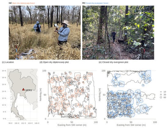
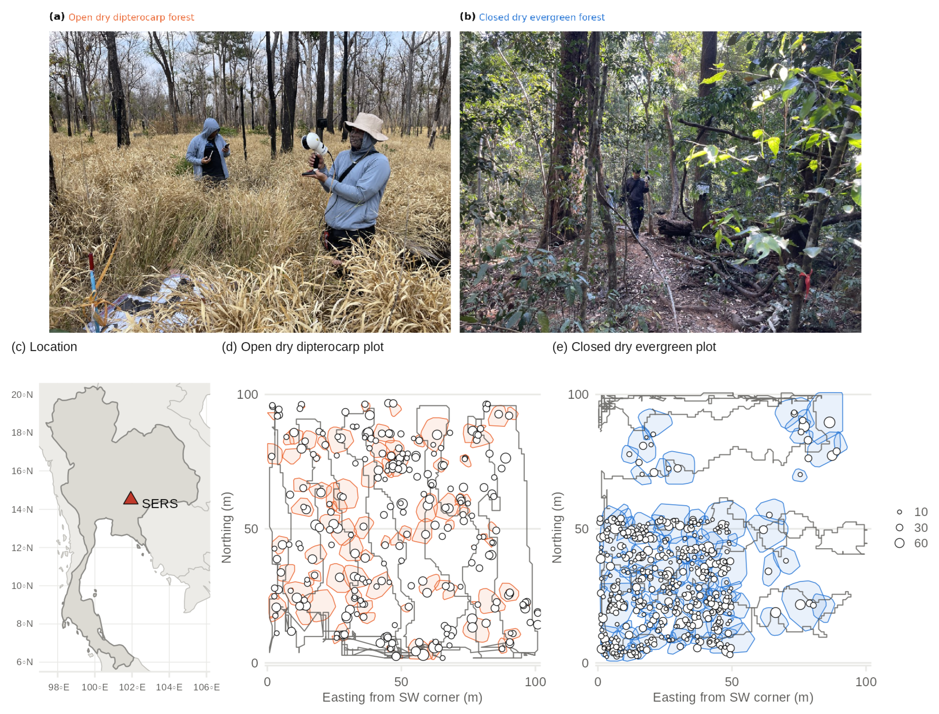
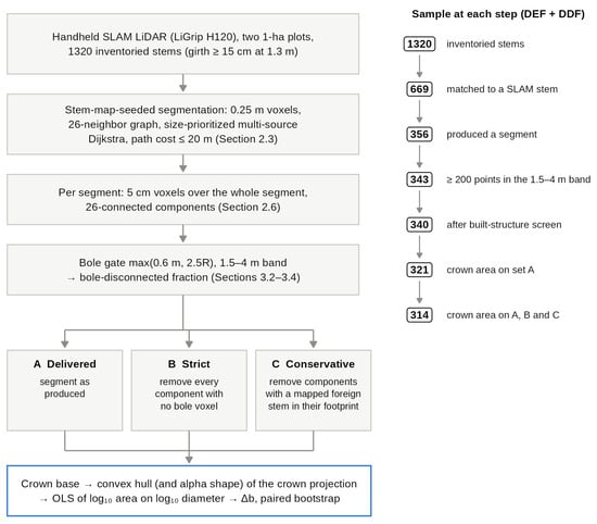
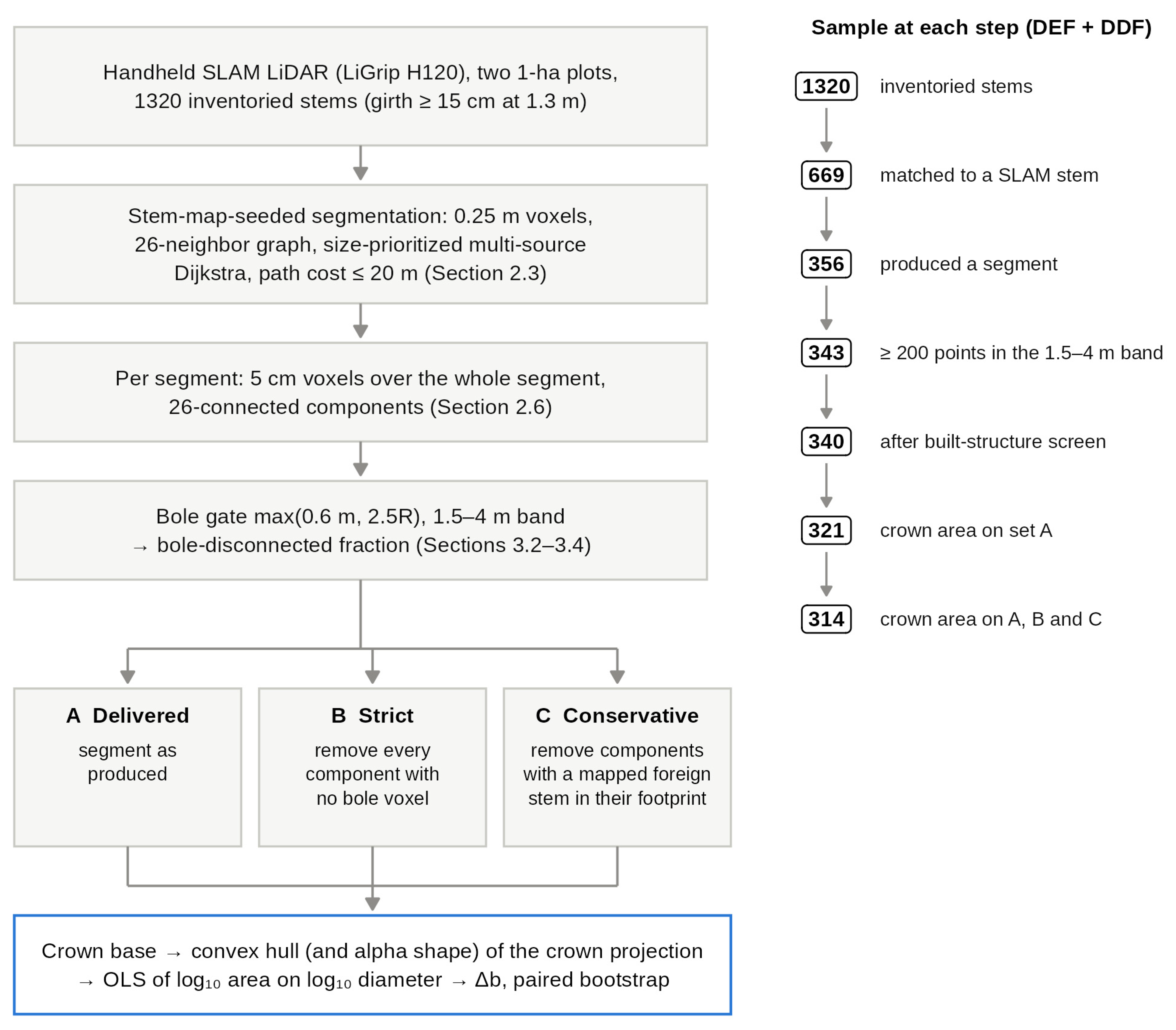
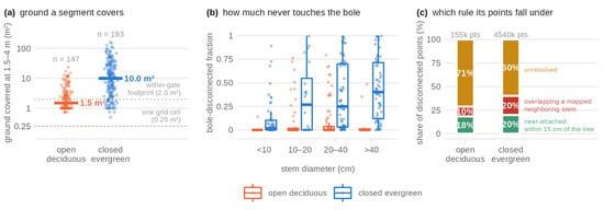
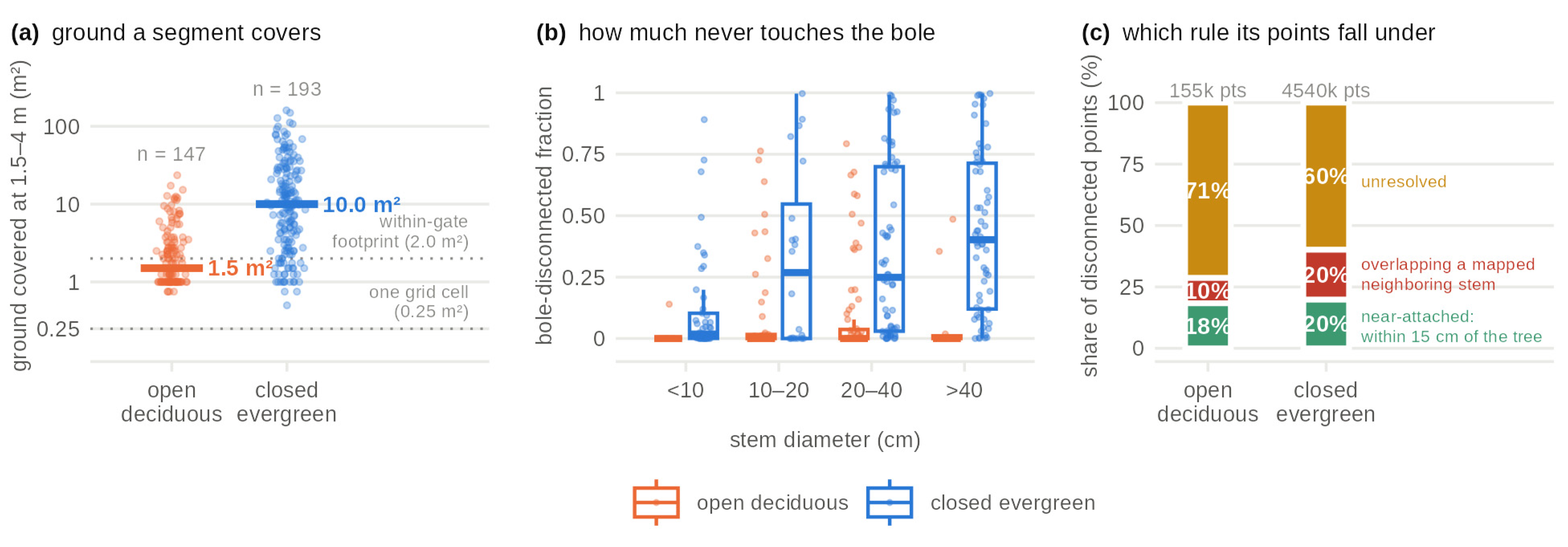
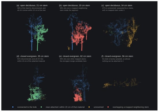
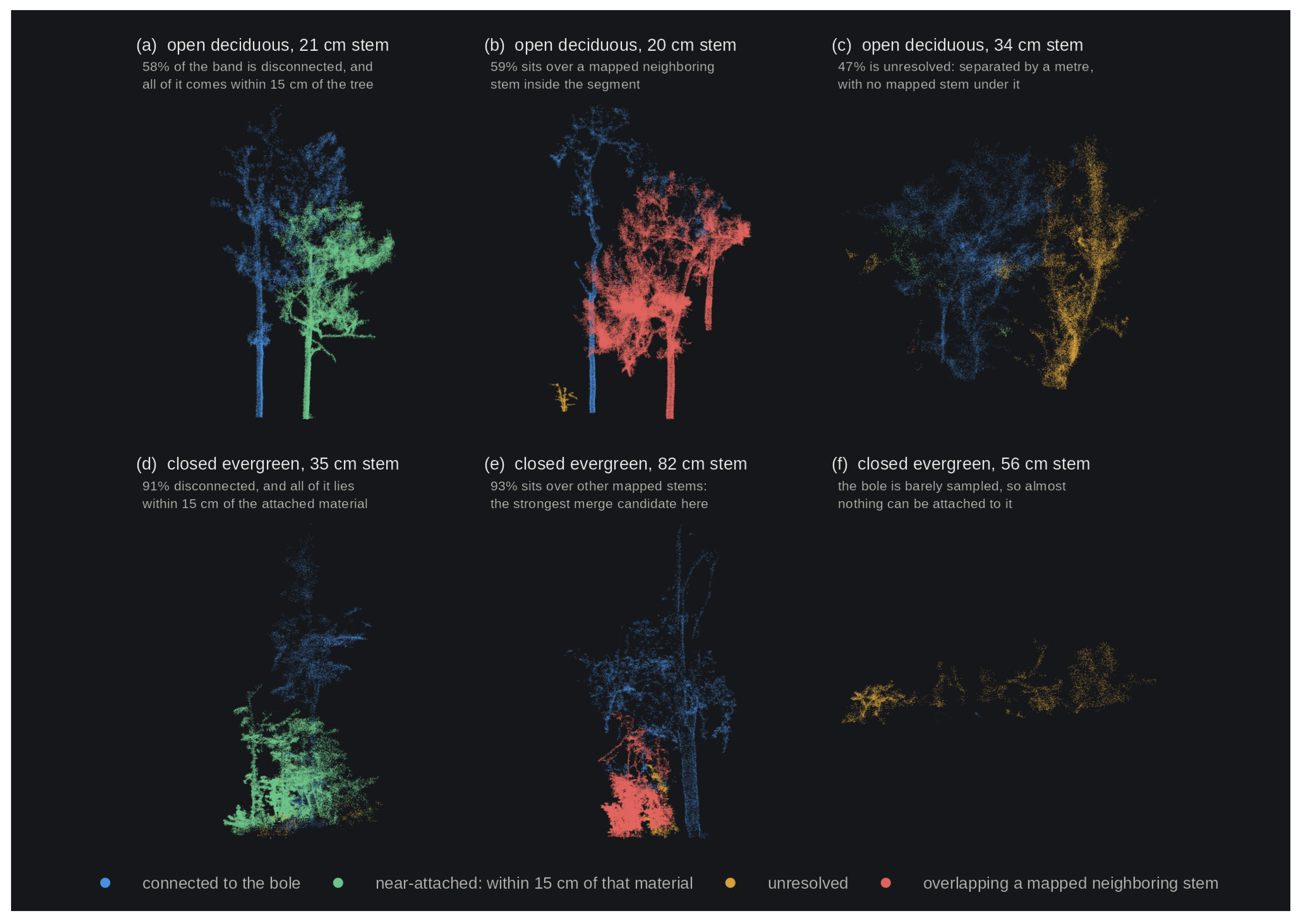
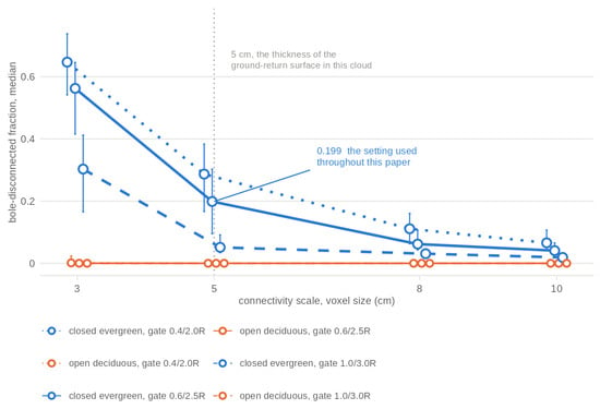
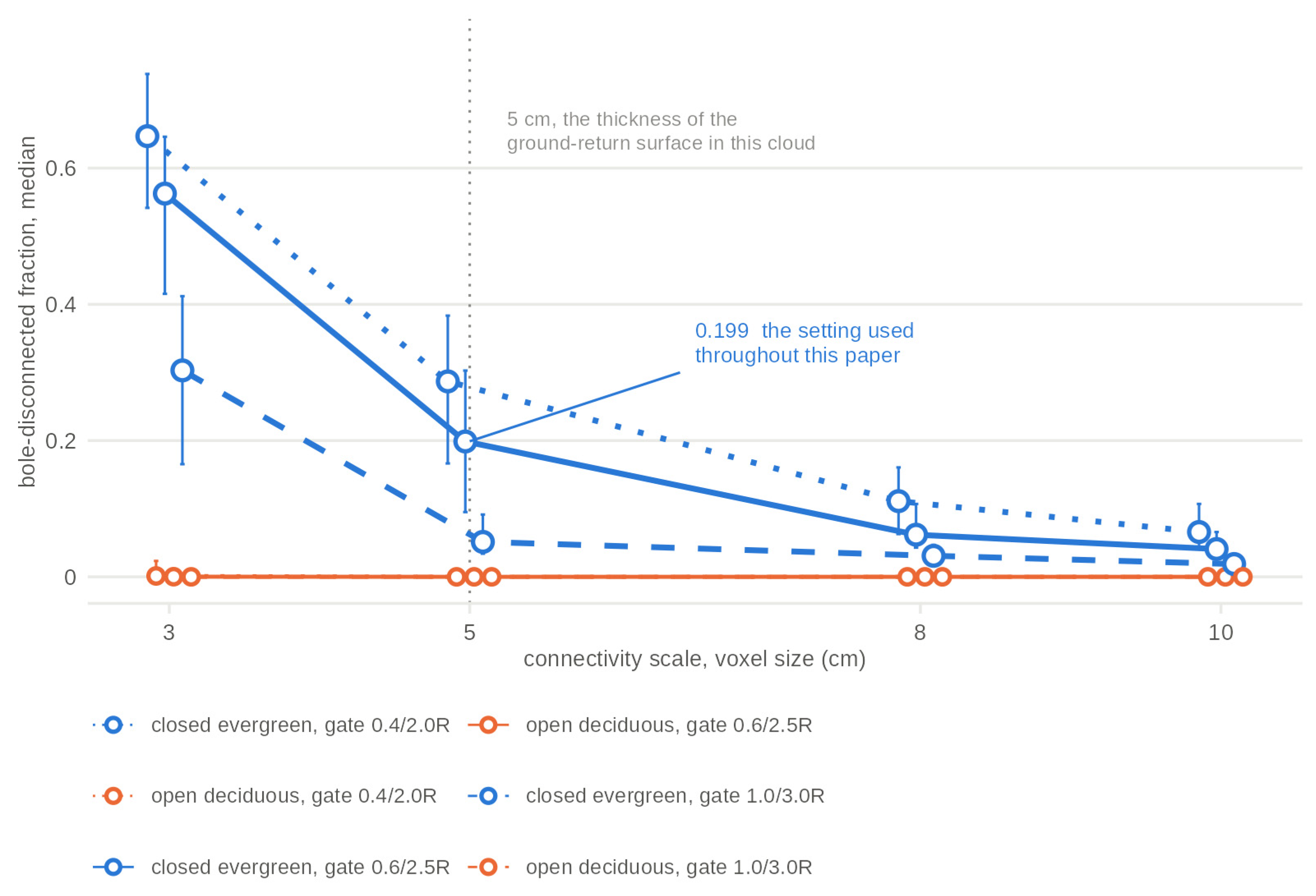
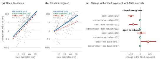
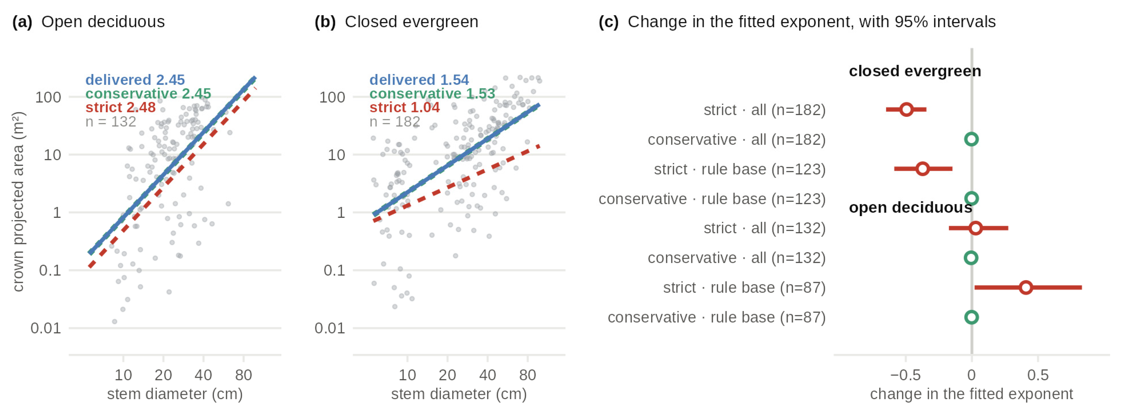
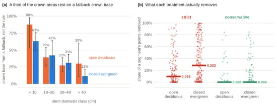
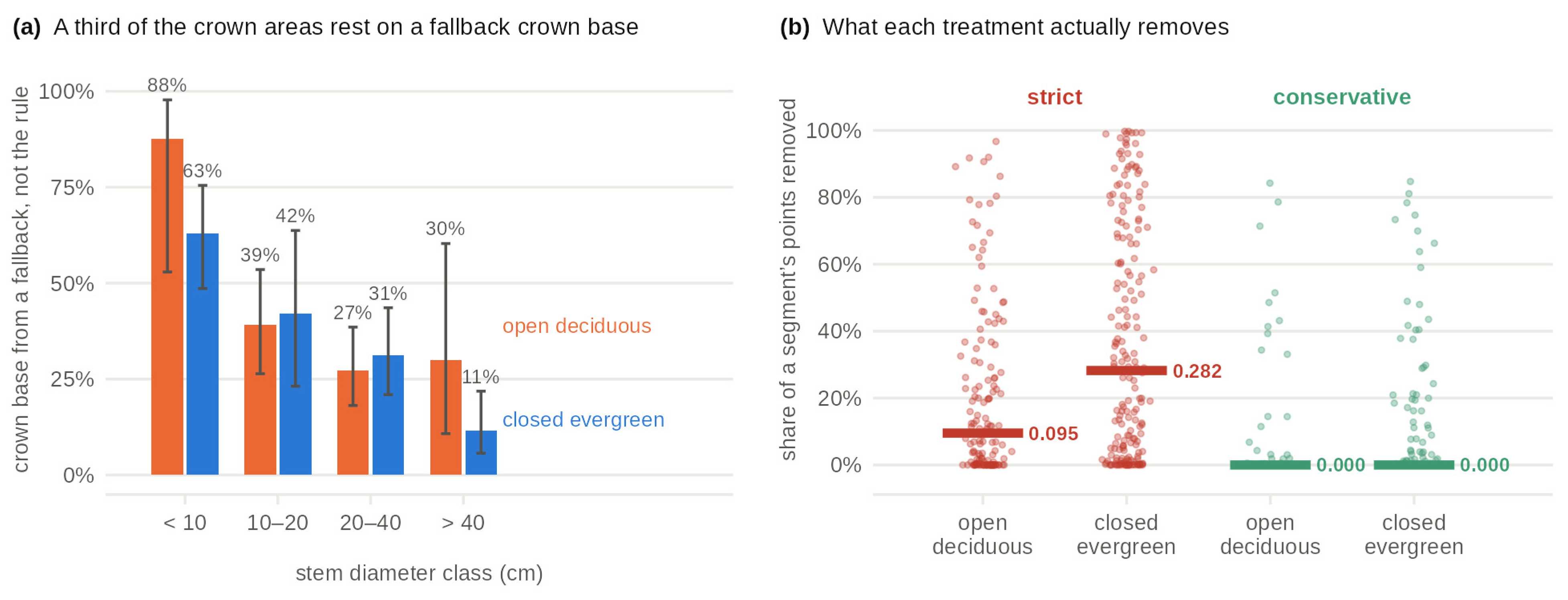

Disclaimer/Publisher’s Note: The statements, opinions and data contained in all publications are solely those of the individual author(s) and contributor(s) and not of MDPI and/or the editor(s). MDPI and/or the editor(s) disclaim responsibility for any injury to people or property resulting from any ideas, methods, instructions or products referred to in the content. |
© 2026 by the authors. Licensee MDPI, Basel, Switzerland. This article is an open access article distributed under the terms and conditions of the Creative Commons Attribution (CC BY) license.