Diurnal Evaluation of AOD-Based Surface Visibility Estimation Using FY-4B Geostationary Observations

Highlights

What are the main findings?

• The simplified AOD-to-visibility conversion exhibits pronounced diurnal variations in estimation errors, with the largest errors occurring at 06 UTC. It also exhibits an underestimation of surface visibility under high-RH conditions.
• Combining empirical RH adjustment with XGBoost residual learning improves visibility estimation, achieving RMSEs of 2.80 km in sample-based cross-validation and 3.10 km in independent-year validation.

What are the implications of the main findings?

• Integrating simplified physical estimates with empirical RH adjustment and residual learning offers a practical approach to satellite-AOD-based surface visibility estimation.
• High-frequency FY-4B observations offer new opportunities for monitoring diurnal variations in surface visibility.

Abstract

Satellite-AOD-based visibility estimation has largely focused on daily-scale estimates or limited overpass times, while its diurnal variations are less understood and discussed. This study therefore investigates surface visibility estimations over China during daytime at 00, 03, 06, and 09 UTC (i.e., 08:00, 11:00, 14:00, and 17:00 China Standard Time, UTC+8), using aerosol optical depth (AOD) observations from the geostationary FY-4B satellite and ERA5 meteorological data. A physically informed framework combines a first-order physical visibility estimate based on AOD, an empirically calibrated relative humidity (RH) adjustment, and XGBoost residual learning. The complete framework, evaluated against ground-based NCEI visibility observations, achieved R = 0.84, RMSE = 2.80 km, and MAE = 2.28 km under sample-based five-fold cross-validation. Independent validation from July 2024 to June 2025 yielded R = 0.79, RMSE = 3.10 km, and MAE = 2.56 km. Visibility-estimation accuracy varied across daytime observation times, with relatively lower errors at 00 and 03 UTC and the largest errors at 06 UTC in both the first-order physical estimate and the final model. Although the complete framework yielded RMSE values of 2.63–3.68 km across the four time slots, these diurnal differences remained evident. The physical estimate also exhibited RH-dependent bias, overestimating visibility at lower RH and underestimating it at higher RH, with a transition near 50%. An empirical RH-conditioned adjustment further reduced estimation errors. These findings highlight the importance of accounting for diurnal and RH-dependent errors in simplified AOD-to-visibility conversion and demonstrate the potential of repeated geostationary observations for daytime surface visibility estimation.

1. Introduction

Atmospheric visibility is a critical indicator of air quality and atmospheric transparency [1]. Meteorologically, it is defined as the maximum horizontal distance at which an observer with normal vision can discern and identify objects against the sky under prevailing weather conditions. Reduced visibility, primarily driven by fog, haze, and smoke, exerts substantial impacts on human health, environmental quality, and the operational efficiency of transportation systems [2,3]. Consequently, robust visibility monitoring remains a high-priority issue in both meteorology and in transportation management.

Conventionally, ground-based visibility monitoring has relied on human observers and on horizontal visibility meters at meteorological stations. While these measurements offer high accuracy, they are constrained by sparse station distribution and limited spatial coverage [4]. This is particularly problematic during large-scale or rapid-evolving low-visibility events, where ground observations fail to provide timely warnings or comprehensive monitoring [5]. To overcome these spatial limitations, satellite remote sensing is increasingly applied to provide long-term observations over wide spatial scales. The physical link between visibility and atmospheric properties is rooted in Koschmieder’s law, which relates horizontal visibility to the atmospheric extinction coefficient at visible wavelengths to which the human eye is sensitive [6]. Atmospheric aerosols, small particles or droplets suspended in the air, are the primary contributors to the extinction at these wavelengths. Aerosol extinction is the sum of scattering and absorption by these particles, determined by their physical and chemical properties—such as size distribution, composition, and hygroscopicity. In high-humidity environments, hygroscopic aerosol particles grow due to condensation of water vapor, which significantly enhances scattering and further degrades visibility [7,8]. Consequently, by establishing relationships between visibility, extinction coefficients, and aerosol optical depth (AOD, i.e., the extinction integrated over the whole vertical atmospheric column), aerosol information retrieved from satellite observation at visible wavelengths can be linked to horizontal surface visibility. Numerous studies have demonstrated the feasibility of satellite-based visibility estimation based on these principles. For instance, Retalis et al. [9] demonstrated a significant correlation between MODIS AOD and near-surface visibility observations, indicating the effectiveness of using AOD to characterize atmospheric transparency. Kessner et al. [10] utilized long-term Automated Surface Observing System (ASOS) data to investigate the relationship between MODIS AOD and near-surface extinction coefficients. Lee et al. [11] proposed an analytical estimation method using a priori aerosol scale height to determine exponential extinction profiles. These studies support the use of satellite AOD as a first-order indicator for visibility estimation.

Visibility is influenced by aerosol properties along the line of sight, which in turn are influenced by meteorological factors such as relative humidity (RH), boundary layer height, and wind speed. These meteorological factors can contribute to substantial variability in the relationship between AOD and surface visibility [12]. To account for these complex relationships, machine-learning approaches have also been applied to satellite-based visibility estimation. For example, Shan et al. [13] utilized neural networks to generate gridded visibility products from satellite-based optical thickness and reanalysis meteorological variables, reporting a mean error of less than 8%. He et al. [14] integrated a first-order physical estimate with machine-learning-based residual correction to produce global visibility estimates from MODIS AOD and reported a correlation coefficient of 0.85, an RMSE of 2.7 km.

These satellite-AOD-based visibility studies relied on polar-orbiting observations acquired at limited local overpass times. However, the relationship between AOD and surface visibility may vary considerably throughout the day [12]. In contrast, geostationary satellites, such as FY-4B, deliver high-frequency observations and have great potential to characterize daytime aerosol variations.

Although satellite AOD reflects aerosol extinction under ambient humidity conditions, estimating surface visibility from AOD depends on the vertical distribution of aerosol extinction. Vertical variations in RH, together with the nonlinear and aerosol-dependent response of light scattering to humidity [15], may introduce additional uncertainty into simplified physical conversion [15,16]. However, relatively few studies have examined the use of physically informed conversion and RH-conditioned adjustments to mitigate these discrepancies in surface visibility estimation

To investigate these issues, this study uses AOD observations during different times of the day from the geostationary FY-4B AGRI sensor and ERA5 meteorological data to estimate surface visibility over China. A first-order physical estimate is constructed to examine estimation errors across different daytime observation times. An empirically calibrated RH-conditioned adjustment is then introduced to address the RH-dependent systematic bias in the initial visibility estimate, followed by XGBoost residual learning to correct the remaining errors. The framework is evaluated through ablation experiments, comparisons with direct XGBoost regression, multiple cross-validation strategies, and an independent 12-month validation. The independent-year evaluation further assesses the temporal generalization of the proposed framework and its applicability to subsequent observations. The study then discusses the limitations of using geostationary satellite AOD for quantitative surface visibility mapping. This work also provides an independent satellite-based reference dataset under cloud-free conditions to complement ground observations and machine learning fused visibility products for regional atmospheric monitoring.

2. Data

2.1. FY-4B AGRI AOD Data

The Advanced Geostationary Radiation Imager (AGRI) onboard the Fengyun-4B (FY-4B) satellite provides aerosol optical depth (AOD) products at 550 nm with a 15 min temporal and 4 km spatial resolution, covering China and its adjacent regions. The officially released Land Aerosol (LDA) products have been operationalized for aerosol monitoring across Asia. In this study, FY-4B LDA AOD data from July 2023 to June 2025 were used. Data from July 2023 to June 2024 were used for model development, model training and internal cross-validation, whereas data from July 2024 to June 2025 were reserved for independent validation. During preprocessing, we retained only on-the-hour observations and high-quality pixels with a Data Quality Flag (DQF) of 3 (good).

2.2. AERONET Data

The Aerosol Robotic Network (AERONET), a global ground-based sun photometer network [17], provides high-quality aerosol observations which are widely used as a reference for validation of satellite AOD products [18,19]. AERONET sites located in China and neighboring Asian regions were retained for analysis. The eligible Level 1.5 (cloud-screened and quality-controlled) measurements must include both 440 nm and 675 nm records for 2024, with sufficient valid temporal overlap relative to quality-controlled, collocated FY-4B AOD retrievals. This procedure resulted in 11 AERONET sites used for FY-4B AOD validation. These AERONET observations were used exclusively for validation of the FY-4B AOD product and were not included in visibility model development or evaluation. Since AERONET does not provide AOD at 550 nm directly, we derived the 550 nm AOD using the Ångström exponent interpolation method [20] between the 440 nm and 675 nm channels, as shown in Equation (1):

$${\mathit{\tau }}_{550}={\mathit{\tau }}_{440}\times {\left({\displaystyle \frac{550}{440}} \right)}^{\mathit{ln}\left({\displaystyle \frac{{\mathit{\tau }}_{440}}{{\mathit{\tau }}_{675}}}\right)/\mathit{ln}\left({\displaystyle \frac{440}{675}}\right)}$$

(1)

For the validation of the FY-4B LDA AOD product, FY-4B and AERONET observations were colocated in space and time. FY-4B AOD data within a 15 km radius of each AERONET site were averaged, and AERONET observations within a ±15 min window centered on the FY-4B observation time were averaged. Only collocated pairs with valid FY-4B DQF values and available AERONET AOD at 550 nm were retained for the validation analysis.

2.3. Meteorological Data

Hourly meteorological variables were obtained from the ERA5 reanalysis product provided by the European Centre for Medium-Range Weather Forecasts (ECMWF). These data, provided at a 0.25° resolution, include key variables such as relative humidity (RH), 2 m temperature (T_s), 10 m wind speed (WS), and planetary boundary layer height (PBLH). These factors significantly modulate near-surface aerosol extinction coefficients [21]. Specifically, RH enhances light scattering via aerosol hygroscopic growth [15], while T_s influences pollutant dispersion through its effect on convection [22]. WS and wind direction govern the transport and dilution of pollutants [23], while PBLH serves as a critical parameter for linking vertical columnar AOD to surface-level horizontal extinction coefficients [16]. For gridded visibility estimation, the ERA5 meteorological fields were spatially interpolated from their original 0.25° grid to the approximately 4 km FY-4B AOD grid, ensuring spatial consistency among the model inputs.

2.4. NCEI Visibility Data

In situ surface visibility observations were obtained from the National Centers for Environmental Information (NCEI) ground station records, which compiles surface meteorological observations from multiple sources and applies quality-control procedures [24]. This dataset was used in this study to provide 3-hourly visibility observations from stations across China, corresponding to the 00, 03, 06, and 09 UTC observation slots. For visibility model development and evaluation, NCEI visibility observations were collocated with FY-4B AOD and ERA5 meteorological variables according to station location and observation time. FY-4B AOD pixels within a 15 km radius of each NCEI station were averaged. ERA5 meteorological variables were bilinearly interpolated to each station location. Only matched samples with valid FY-4B AOD, valid meteorological variables, and visibility smaller than 30 km, and RH below 90% were retained. Samples with missing AOD retrievals, invalid DQF values, missing meteorological variables, or unavailable visibility records were excluded.

2.5. Study Area and Station Distribution

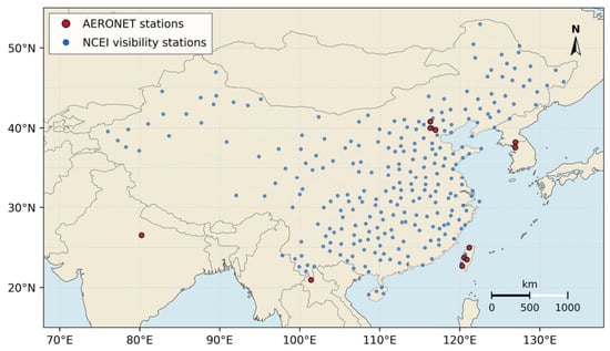
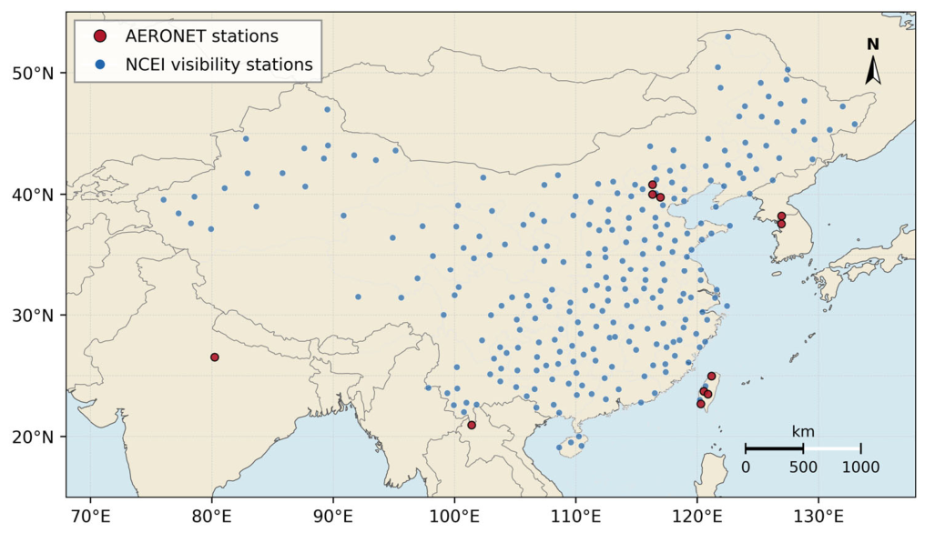
The visibility estimation focuses on China, while AERONET data used for FY-4B AOD validation are obtained from sites in China and neighboring Asian regions. Figure 1 shows the spatial distribution of the AERONET stations used for FY-4B AOD validation and the NCEI stations used for visibility model development and evaluation.

Figure 1. Study area and spatial distribution of the AERONET stations used for FY-4B AOD validation and the NCEI stations used for visibility model development and evaluation. AERONET data from sites outside China were retained solely for FY-4B AOD validation.

3. Methodology

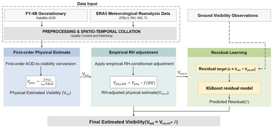
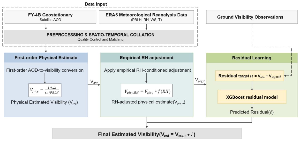
To support regional-scale diurnal visibility estimation, we developed a framework that integrates geostationary FY-4B AOD observations with ERA5 meteorological data. As illustrated in Figure 2, the framework consists of three sequential components: a first-order physical estimate, an empirically calibrated RH-conditioned adjustment, and XGBoost-based residual learning. The physical estimate provides an approximate conversion from column-integrated AOD to near-surface visibility under simplified assumptions regarding aerosol vertical distribution and near-surface extinction. The RH adjustment further modifies this physical prior according to the ambient RH condition, with its parameters determined using an isolated calibration subset and fixed before subsequent model training and evaluation. The residual-learning stage then estimates the remaining discrepancy between the adjusted physical prior and ground-observed visibility using the physical estimate together with aerosol, meteorological, and temporal predictors. The final visibility estimate is obtained by adding the predicted residual to the adjusted physical prior. A direct XGBoost model is additionally evaluated as a purely data-driven benchmark using the same original predictors without the physical-prior input. The detailed formulations and evaluation procedures are described in Section 3.1, Section 3.2, Section 3.3 and Section 3.4.

Figure 2. Framework of the physically informed residual-learning approach, including the first-order physical estimate, empirical RH-conditioned adjustment, and data-driven residual-learning components.

3.1. First-Order Physical Estimate

The first stage of the framework is designed to construct a first-order physical estimate linking satellite-derived AOD with near-surface visibility. It should be noted that this stage is not intended to provide a complete deterministic retrieval of visibility. Satellite AOD is a wavelength-dependent column-integrated quantity, whereas surface visibility is controlled by horizontal extinction along the near-surface optical path and is related to visual or instrumental response. Therefore, the AOD–visibility relationship used here should be interpreted as an approximate conversion under simplifying assumptions regarding wavelength representativeness, aerosol vertical distribution, horizontal homogeneity, and near-surface mixing.

The physical estimate is constructed following the analytical framework established by He et al. [14], based on optical extinction theory and Koschmieder’s law, which, under horizontally homogeneous conditions, relates horizontal visibility to the near-surface extinction coefficient through a contrast threshold:

$$V = -{\displaystyle \frac{ln(C_T)}{{\mathit{\beta }}_{ext }\left(0\right)}}$$

(2)

where V is horizontal visibility, $C_T$ is the contrast threshold, and ${\mathit{\beta }}_{ext }\left(0\right)$ is the near-surface extinction coefficient. When $C_T=0.02$, −ln(C_T) is approximately 3.912, yielding the commonly used form:

$$V = {\displaystyle \frac{3.912}{{\mathit{\beta }}_{ext }\left(0\right)}}$$

(3)

In the physical estimate, the near-surface extinction term is approximated using aerosol extinction inferred from AOD. The aerosol extinction coefficient at height z and wavelength λ can be expressed as the product of aerosol number concentration and an effective extinction cross-section:

$${\mathit{\beta }}_{ext}\left(z\right)= N_z\ast {\mathit{\sigma }}_{ext}$$

(4)

where $N_z$ is the aerosol number concentration at height z, and ${\mathit{\sigma }}_{ext}$ represents the effective aerosol extinction cross-section at 550 nm. At the surface, this relationship can be written as:

$${\mathit{\beta }}_{ext}\left(0\right)= N_0\ast {\mathit{\sigma }}_{ext}$$

(5)

where $N_0$ is the near-surface aerosol number concentration. For the first-order physical estimate, ${\mathit{\sigma }}_{ext}$ is assumed to be vertically invariant within the effective aerosol layer. Under this assumption, the vertical variation in aerosol extinction is mainly controlled by the vertical variation in aerosol number concentration:

$${\displaystyle \frac{{\mathit{\beta }}_{ext\left(Z\right)}}{{\mathit{\beta }}_{ext\left(0\right)}}}={\displaystyle \frac{N_z}{N_0}}$$

(6)

Typically, aerosol number concentration is assumed to decrease exponentially with height:

$$N_z=N_0\ast e^{-{\displaystyle \frac{z}{H}}}$$

(7)

where H is the aerosol scale height. Under this exponential vertical distribution assumption, the aerosol extinction profile can be written as:

$${\mathit{\beta }}_{ext}(z)= {\mathit{\beta }}_{ext}(0)\ast e^{-{\displaystyle \frac{z}{H}}}$$

(8)

The corresponding column AOD is then obtained by vertically integrating the aerosol extinction coefficient:

$${\mathit{\tau }}_a= {\int }_0^{\infty }{\mathit{\beta }}_{ext}\left(z\right) dz$$

(9)

where ${\mathit{\tau }}_a$ is AOD at 550 nm. Integrating this exponential extinction profile over height gives:

$${\mathit{\tau }}_a={\int }_0^{\mathrm{\infty }}{\mathit{\beta }}_{ext}(0)\ast e^{-{\displaystyle \frac{z}{H}}}dz={\mathit{\beta }}_{ext}(0)\ast H$$

(10)

Thus, the near-surface aerosol extinction coefficient can be approximated as:

$${\mathit{\beta }}_{ext}(0)\approx {\displaystyle \frac{{\mathit{\tau }}_a}{H}}$$

(11)

Under an exponentially decreasing aerosol profile, the column AOD can be expressed as the product of near-surface aerosol extinction and an effective aerosol scale height. Previous satellite-based column-to-surface aerosol studies have used boundary-layer height to represent this vertical scaling [25,26], and this approximation has also been adopted in satellite-based surface-visibility estimation [16]. Accordingly, in the present first-order conversion, H is represented by PBLH as a pragmatic effective scale-height proxy rather than as the actual aerosol layer height.

$${\mathit{\beta }}_{ext}(0)\approx {\displaystyle \frac{{\mathit{\tau }}_a}{PBLH}}$$

(12)

Combining this extinction approximation with Koschmieder’s law, the first-order physical visibility estimate can be expressed as:

$$V_{phy}={\displaystyle \frac{3.912}{{\mathit{\tau }}_a/PBLH}}$$

(13)

This formulation is used as a simplified first-order physical prior rather than a complete physical retrieval of surface visibility. Its applicability depends on the representativeness of the assumed aerosol vertical profile and effective scale height. In particular, the PBLH-based approximation may become less representative when residual aerosol layers, elevated dust or smoke, or strong vertical stratification are present. Other variations in aerosol optical and microphysical properties are likewise not explicitly resolved at this stage and contribute to the remaining discrepancy addressed by the subsequent empirical RH adjustment and residual-learning model.

3.2. Empirical RH-Conditioned Adjustment

The RH adjustment is applied to the first-order visibility estimate rather than to satellite AOD, which already represents aerosol extinction under ambient humidity conditions. Motivated by the potential RH dependence of errors in the simplified column-to-surface conversion, an empirical RH-conditioned factor is introduced to refine the initial visibility estimate before residual learning. This adjustment is intended to reduce systematic estimation bias, not to explicitly retrieve aerosol hygroscopic growth or vertical humidity structure.

To represent this RH dependence in a continuous form, a normalized power-law relationship motivated by earlier visibility–humidity parameterizations [27] was adopted:

$$f(RH) = {\left({\displaystyle \frac{1-RH/100}{1-R{H}_0/100}}\right)}^{\mathit{\gamma }}$$

(14)

where RH denotes near-surface relative humidity used as an ERA5 meteorological input in this study, RH₀ is the reference humidity, and $\mathit{\gamma }$ is an empirically calibrated sensitivity parameter controlling the direction and magnitude of the adjustment. The normalization gives $f\left({RH}_0\right)$ = 1, with RH₀ serving as the reference RH value at which no adjustment is applied rather than a physical hygroscopic threshold.

The adjusted physical estimate is then expressed as:

$$V_{phy,RH}=V_{phy}f\left(RH\right)$$

(15)

The parameters were determined using an isolated RH-calibration subset, which was excluded from subsequent model training and cross-validation. The RH-conditioned adjustment was applied only to samples with RH above 30%. The reference humidity was selected according to the RH dependence of the mean bias in the first-order physical estimate. Both parameters were then fixed before subsequent model training, cross-validation, and independent validation. The calibrated $\mathit{\gamma }$ is treated as an empirical sensitivity parameter rather than a directly measured aerosol hygroscopicity coefficient.

3.3. Residual Model

Although the RH-adjusted physical estimate provides a first-order estimate of visibility, systematic deviations remain in practical applications. These deviations may arise from simplified assumptions regarding aerosol vertical distribution, uncertainties in satellite AOD and PBLH, unresolved aerosol microphysical properties, and meteorological effects that are not fully represented in the physical estimate. To address these deviations, this study introduces an XGBoost-based residual correction after the RH-adjustment stage. Defining the observed near-surface visibility as $V_{obs}$ and the modeled visibility as V_phy,RH, the residual ε can be expressed as:

$$\epsilon =V_{obs}-V_{phy,RH}$$

(16)

We utilize Extreme Gradient Boosting (XGBoost) as the residual learning model, which is a gradient-boosted decision-tree algorithm that has been widely used for nonlinear regression tasks because of its ability to represent complex feature interactions and its built-in regularization strategy [28]. The predicted residual can be expressed as:

$$\widehat{\epsilon }=F_{XGB}\left(X\right)$$

(17)

where X denotes the input feature set of the residual model. The inputs include the RH-adjusted physical visibility estimate V_phy,RH, satellite-derived AOD, meteorological variables including relative humidity, temperature, wind speed, and planetary boundary layer height, and temporal indicators including the day of year and hour. The complete set of input variables is summarized in Table 1.

Table 1. Input variables used in the XGBoost residual correction model.

Category	Variable	Symbol
Physical estimate	Physical-estimate visibility	Vphy,RH
Aerosol	Aerosol optical depth	AOD
Meteorological	Relative humidity	RH
Meteorological	Air temperature	T
Meteorological	Wind speed	WS
Meteorological	Planetary boundary layer height	PBLH
Temporal	Day of year	DOY
Temporal	Hour	Hour

These predictors were selected to represent the first-order physical estimate, aerosol loading, near-surface meteorological and boundary-layer conditions, and recurrent temporal variability. Bayesian optimization was applied to tune key XGBoost hyperparameters, including tree depth, learning rate, and subsampling ratio. An early-stopping strategy was used during model training to reduce overfitting.

The final visibility estimate is then obtained by adding the predicted residual back to the RH-adjusted physical estimate:

$$V_{est}=V_{phy,RH}+\widehat{\epsilon }$$

(18)

In this way, the machine-learning component corrects the remaining errors that are not fully represented by the simplified physical and RH-adjustment stages.

3.4. Model Training and Evaluation Metrics

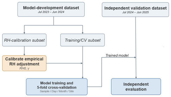
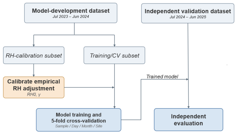
Following the quality-control and collocation procedures described in Section 2, the matched samples with valid FY-4B AOD and RH below 90% were organized into a model-development period (July 2023–June 2024) and a temporally independent validation period (July 2024–June 2025). Samples with RH ≥ 90% were excluded to reduce the influence of near-saturated conditions, where fog or precipitation may complicate the relationship between satellite AOD and surface visibility. Within the development period, an isolated subset comprising 30% of the samples was selected across all stations exclusively to calibrate the RH-adjustment parameters described in Section 3.2. This subset was excluded from subsequent model training and cross-validation. The remaining 16,234 matched samples in the training subset were used for model development and cross-validation, while 25,855 samples from the subsequent year were reserved for independent validation. The data partitioning and separation of the RH-calibration, model-development, and independent-validation subsets are illustrated in Figure 3.

Figure 3. Data-partitioning and model-validation workflow.

This study employs a five-fold cross-validation method to evaluate the model’s generalization performance. Four partitioning strategies were considered: sample-based, day-based, month-based, and site-based cross-validation. In sample-based cross-validation, individual matched samples were randomly assigned to five folds. For the other three strategies, samples were grouped by observation date, calendar month, or station, respectively, so that the corresponding groups did not overlap between training and validation folds. For each strategy, the model was trained using four folds and evaluated on the remaining fold. This procedure was repeated until every sample had received one out-of-fold prediction.

Bayesian hyperparameter optimization and early stopping were conducted independently within each cross-validation training fold, using only data from the corresponding training partition. The held-out fold was reserved exclusively for model evaluation. Following model development, the model was fitted using the development samples and evaluated on the independent validation period, without using the independent validation observations for parameter selection or model fitting.

For benchmark comparison, a direct XGBoost regression model (Direct_XGB) was also evaluated using the same original aerosol, meteorological, and temporal predictors, without the physical estimate as an additional input. Direct_XGB predicted observed visibility directly and was evaluated using the same data partitions and validation procedures as the residual-learning model.

To quantitatively evaluate model precision, we utilize the Root Mean Square Error (RMSE), Correlation Coefficient (R), Mean Absolute Error (MAE), and Bias. These metrics are calculated as follows:

$$RMSE = \sqrt{\left({\displaystyle \frac{1}{N}}\right){\sum }_{i=1}^N{\left(y_i - {\widehat{\mathrm{y}}}_i\right)}^2}$$

(19)

$$R={\displaystyle \frac{{\sum }_{i=1}^N\left(x_i-\overline{x}\right)\left(y_i-\overline{\mathrm{y}}\right)}{\sqrt{{\sum }_{i=1}^N(x_i-\overline{x}{)}^2{\sum }_{i=1}^N(y_i-\overline{\mathrm{y}}{)}^2}}}$$

(20)

$$MAE=\left({\displaystyle \frac{1}{N}}\right)\ast {\sum }_{i=1}^N|y_i-{\widehat{\mathrm{y}}}_i|$$

(21)

$$Bias={\displaystyle \frac{1}{N}}\ast {\sum }_{i=1}^N({\widehat{y}}_i-y_i)$$

(22)

where N represents the total number of samples, $y_i$ denotes the observed visibility, and ${\widehat{\mathrm{y}}}_i$ is the predicted value. Higher R and lower RMSE and MAE, together with a mean bias closer to zero, indicate superior model performance.

For the validation of the FY-4B AOD product against AERONET observations, the Expected Error (EE) envelope is also used to evaluate the consistency between satellite-retrieved AOD and ground-based AOD. Following common satellite AOD validation practice, the EE range is defined as:

$$EE=\pm (0.05+0.15{\mathit{\tau }}_{AERONET})$$

(23)

A FY-4B AOD retrieval is considered to fall within the EE envelope when:

$$\left|{\mathit{\tau }}_{FY4B}-{\mathit{\tau }}_{AERONET}\right|\le 0.05+0.15{\mathit{\tau }}_{AERONET}$$

(24)

where ${\mathit{\tau }}_{FY4B}$ and ${\mathit{\tau }}_{AERONET}$ denote FY-4B and AERONET AOD at 550 nm, respectively. The EE envelope is selected because it accounts for both an absolute error component and an AOD-dependent relative error component, and is commonly used as a reference uncertainty range in satellite AOD validation.

4. Results

4.1. Validation of FY-4B LDA AOD Products

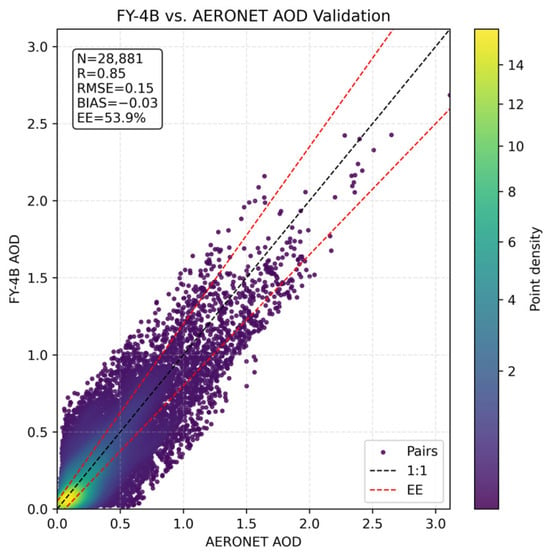
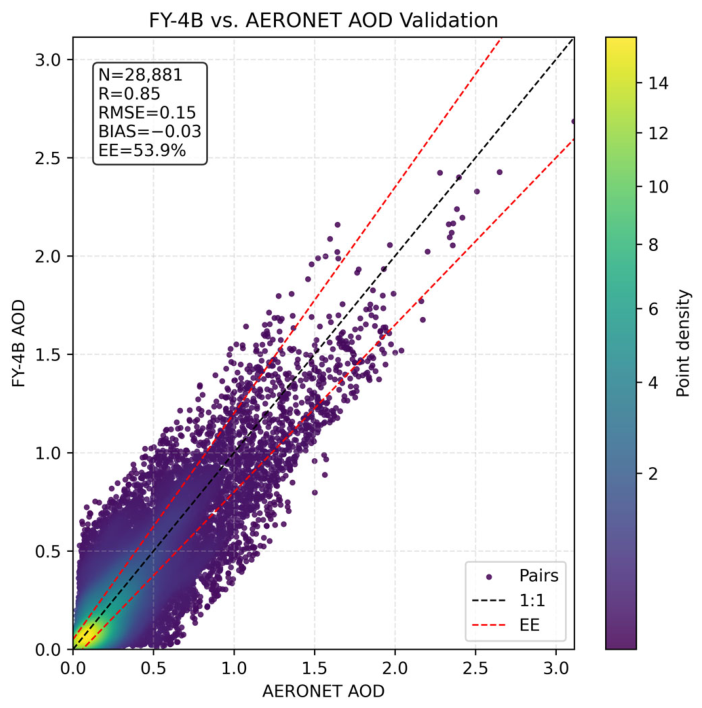
Prior to the visibility estimation, the FY-4B AOD products were evaluated against ground-based AERONET observations, utilizing hourly data from 11 AERONET sites. Based on the quality-control and the procedure described in Section 2.1 and Section 2.2, collocation pairs of FY-4B and AERONET AOD at 550 nm were generated and used to assess the applicability of the FY-4B AOD product for subsequent visibility estimation. The density scatterplot in Figure 4 shows the comparison of the colocated FY-4B and AERONET AOD data for 2024, together with the number of data pairs and the validation metrics mentioned in Section 3.4. The resulting R, RMSE, and bias are 0.85, 0.15, and −0.03, respectively, with approximately 53.9% of the samples falling within the EE envelope.

Figure 4. Scatter density plot of the FY−4B satellite AOD data versus AERONET reference AOD data, both at 550 nm, for 2024.

The hour-by-hour validation results for the FY-4B LDA AOD product versus AERONET data are presented in Table 2. The retrieval performance shows clear temporal variation during the available daytime observation period. The correlation coefficient was highest at 00 UTC (R = 0.92) and again during 08 and 09 UTC (R = 0.92 and 0.91, respectively), while the lowest value occurred at 05 UTC (R = 0.79). The RMSE was lowest at 00 UTC (0.093) and increased to a maximum of 0.175 at 03 UTC, after which it gradually decreased to 0.145–0.152 during 8–9 UTC.

Table 2. Results from the hour-by-hour validation of the FY-4B LDA AOD product versus AERONET reference data.

UTC	N	R	RMSE	BIAS	Within EE
00	2913	0.92	0.093	−0.024	0.74
01	3764	0.89	0.128	−0.021	0.67
02	4078	0.85	0.162	−0.027	0.56
03	3661	0.81	0.175	−0.033	0.48
04	3371	0.81	0.172	−0.012	0.45
05	3263	0.79	0.171	−0.022	0.46
06	3077	0.83	0.162	−0.024	0.50
07	2579	0.87	0.154	−0.051	0.50
08	1772	0.92	0.145	−0.072	0.47
09	403	0.91	0.152	−0.090	0.42

The bias was negative throughout the daytime validation period, ranging from −0.012 to −0.090. The magnitude of the negative bias generally increased toward the end of the available retrieval period, reaching −0.090 at 09 UTC. The fraction of retrievals falling within the EE envelope also decreased from 74% at 00 UTC to 42% at 09 UTC. Meanwhile, the number of matched samples varied substantially among the hourly intervals, decreasing to 403 at the final 09 UTC.

Overall, the FY-4B LDA AOD product showed a relatively strong correlation with AERONET observations. However, the limited fraction of retrievals within the EE envelope and the observed variations in RMSE and bias across daytime intervals indicate non-negligible retrieval uncertainty. These results support the use of FY-4B AOD as an input for subsequent visibility estimation, while also indicating time-dependent retrieval uncertainties that may contribute to visibility estimation errors.

4.2. Visibility Estimation Results

4.2.1. Evaluation of Model Results

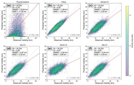
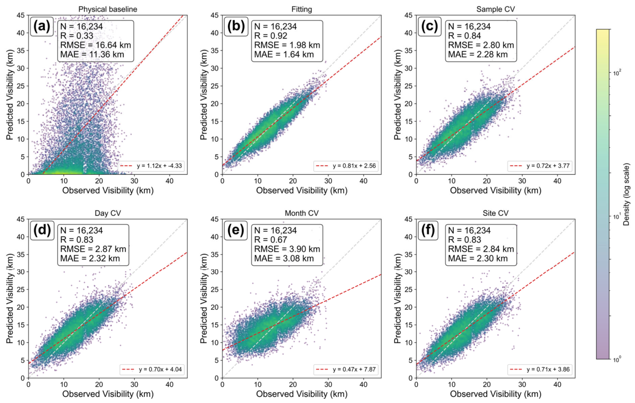
Following the data preprocessing and collocation procedures described in Section 2, 16,234 valid matched samples comprising FY-4B AOD, ERA5 meteorological variables, and NCEI visibility observations were retained and used to evaluate the overall performance of the proposed visibility estimation framework. The isolated RH-calibration subset yielded a reference humidity of RH₀ = 50% based on the RH-dependent mean bias pattern, and γ = −0.22 was selected within the near-minimum range of calibration RMSE. Both parameters were fixed before subsequent model training and evaluation, with the calibration results further examined in Section 4.2.5. To clarify the role of each validation setting, the model performances under progressively different levels of constraint are presented in Figure 5, by comparison of the model results with the observed visibility. Figure 5a shows the results from the standalone physical estimate, i.e., the simplified AOD–extinction–visibility relationship presented by Equation (13). Figure 5b–f all show the final visibility estimates obtained after XGBoost residual correction. Figure 5b presents the full-sample fitting result and is used only as an in-sample diagnostic reference for the fitting capacity of the residual-learning model. Figure 5c shows the standard sample-based five-fold cross-validation result, which provides a conventional estimate of predictive performance on randomly held-out samples. In addition, Figure 5d–f present day-based, month-based, and site-based cross-validation results, respectively, to further assess temporal and spatial generalization.

Figure 5. Evaluation of the different steps of the visibility estimation framework through scatter density plots of the results versus the ground-based observations from the NCEI network: (a) physical mechanism-based model (Phy_Base); (b) in-sample XGBoost residual-corrected estimates (Fitting), (c) 5-fold random sample cross-validation; (d) 5-fold independent day cross-validation; (e) 5-fold independent month cross-validation; (f) 5-fold independent site cross-validation.

The scatter density plot of the results of the physical stage (Phy_Base) based on Koschmieder’s Law versus observed visibility (NCEI data) in Figure 5a clearly shows that the physical estimate alone has poor estimation performance under real atmospheric conditions, with a low correlation and large systematic deviations. After XGBoost residual correction, the in-sample fitting result shown in Figure 5b achieved a correlation coefficient R of 0.92, an RMSE of 1.98 km, and an MAE of 1.64 km. This in-sample result only reflects the fitting capability of the residual model and cannot represent the model’s generalization performance on unseen samples.

Figure 5c presents the results of the sample-based five-fold cross-validation (Sample-based CV). Compared with the full-sample fitting, the model performance decreased, as expected for held-out samples, but retained reasonable predictive accuracy, with R = 0.84, RMSE = 2.80 km, and MAE = 2.28 km. This indicates that the proposed framework retains reasonable predictive performance on randomly held-out samples.

More restrictive temporal and spatial partitioning strategies were further applied to evaluate model generalization (Figure 5d–f). For day-based cross-validation (Day-based CV, Figure 5d) and month-based cross-validation (Month-based CV, Figure 5e), samples were partitioned into training and validation folds according to their observation dates and calendar months, respectively. The results were R = 0.83, RMSE = 2.87 km, and MAE = 2.32 km for the day-based approach, and R = 0.67, RMSE = 3.90 km, and MAE = 3.08 km for the month-based approach. Among the four cross-validation strategies, the month-based partition produced the lowest performance, indicating that generalization across temporally separated monthly subsets is more challenging than generalization across randomly held-out samples or days. In the spatial dimension, the result for site-based cross-validation (Site-based CV, Figure 5f) was R = 0.83, RMSE = 2.84 km, and MAE = 2.30 km, indicating that the model retains a reasonable level of spatial transferability across stations. Overall, Figure 5 demonstrates that the physical estimate alone is not suitable for direct visibility retrieval, while the residual-learning framework substantially improves estimation accuracy, although performance decreases under month-based validation.

4.2.2. Diurnal Variation in Visibility Estimation

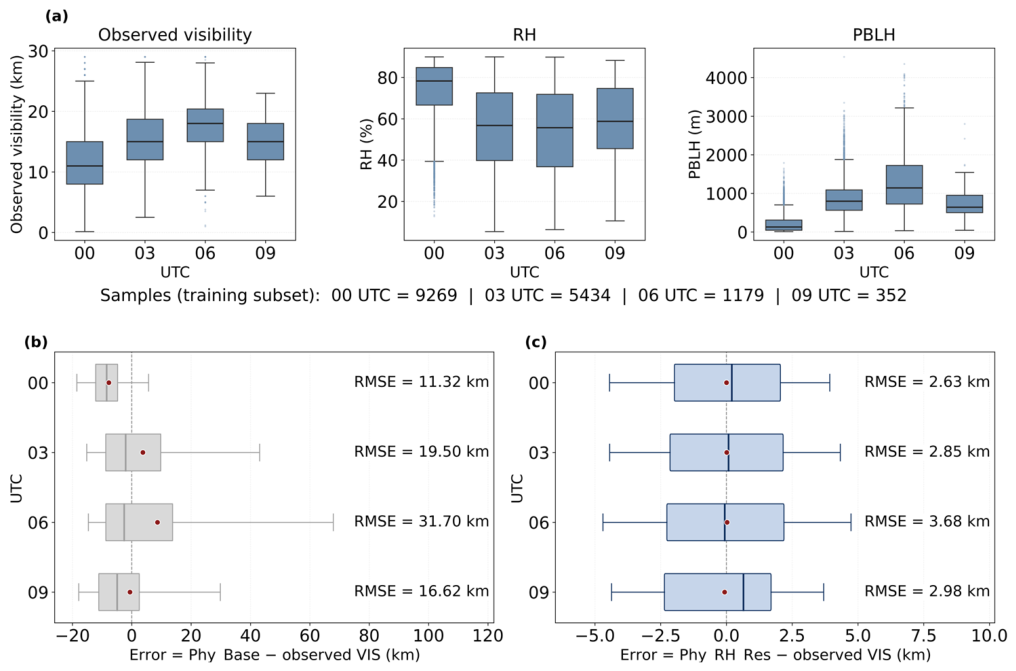
Diurnal variations in visibility-estimation performance are examined using the same model-development samples as in Section 4.2.1, grouped by observation time (00, 03, 06, and 09 UTC) (Figure 6). The evaluation of the final model was based on out-of-fold predictions from sample-based five-fold cross-validation.

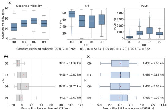
Figure 6. Diurnal variations in atmospheric conditions and visibility-estimation errors: (a) distributions of observed VIS, RH, and PBLH; (b) error distributions of Phy_Base; and (c) error distributions of Phy_RH_Res. Boxes indicate Q1–Q3, whiskers indicate P5–P95, red dots indicate means, and dashed lines indicate zero error. RMSE values are annotated for each UTC group.

The observed atmospheric conditions varied across the four time slots (Figure 6a). The numbers of samples in the training subset were 9269, 5434, 1179, and 352 at 00, 03, 06, and 09 UTC, respectively, indicating substantially fewer valid matches at the later observation times. From 00 to 06 UTC, median observed visibility increased from 11 to 18 km, while median RH decreased from 78.3% to 55.7% and median PBLH increased from approximately 129 to 1141 m. These results indicate differences in the observed atmospheric conditions and sample availability among the UTC groups.

The first-order physical estimate (Phy_Base) showed pronounced differences in error distributions across observation times (Figure 6b). The mean bias changed from −7.71 km at 00 UTC to positive values at 03 and 06 UTC, although the median errors remained negative, indicating the influence of relatively large positive errors. The most notable deterioration occurred at 06 UTC, where the error distribution broadened considerably and RMSE reached 31.70 km, compared with 11.32 km at 00 UTC.

After RH adjustment and XGBoost residual learning, the errors became more tightly clustered around zero, with substantially narrower and more consistent distributions across the four time slots (Figure 6c). RMSE ranged from 2.63 km at 00 UTC to 3.68 km at 06 UTC. Thus, the final model substantially reduced the error magnitude and narrowed the diurnal differences, although the errors remained relatively higher at 06 UTC.

4.2.3. Spatial and Seasonal Variations in Estimation Accuracy

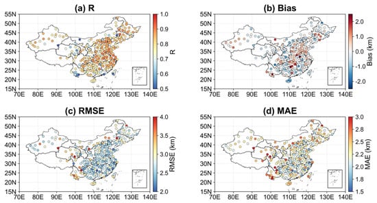
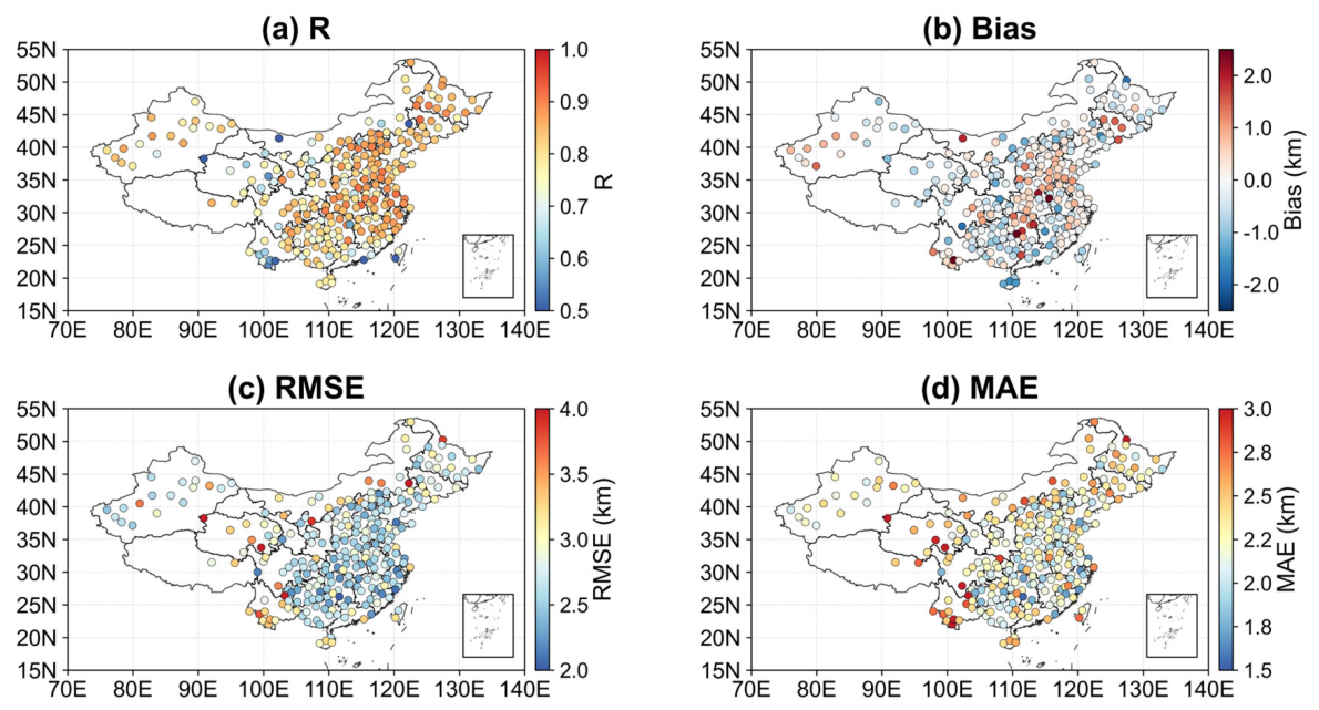
To further evaluate the spatial variation in model performance across China, Figure 7 presents the spatial distributions of R, mean bias, RMSE and MAE for each site, where the mean bias is defined as the estimated visibility minus the observed visibility. Overall, the site-level metrics indicate clear spatial heterogeneity in model performance. The R values are generally higher over eastern and central China, indicating more consistent agreement between estimated and observed visibility at many stations in these regions. In contrast, lower R values are more frequently observed over western China and at several southeastern coastal stations.

Figure 7. Spatial distribution of visibility and site-specific validation metrics across China during July 2023–June 2024: (a) R; (b) mean bias; (c) RMSE (km); (d) MAE (km).

In Figure 7b, negative biases indicate an underestimation of visibility and are more evident in southern and southwestern China, whereas positive biases are more frequently observed in Central China and North China, with additional scattered positive biases in northeastern and northwestern China. The spatial distributions of RMSE and MAE show broadly consistent patterns, indicating that the magnitude of absolute errors also varies regionally. Lower RMSE and MAE values are observed at many stations in southeastern and central-eastern China, whereas larger errors occur more frequently at stations in western and northwestern China, northeastern China, and several coastal locations. Overall, Figure 7 indicates that the station-level model performance is generally better over many eastern and central-eastern stations, with larger uncertainties in western, northeastern, and coastal stations.

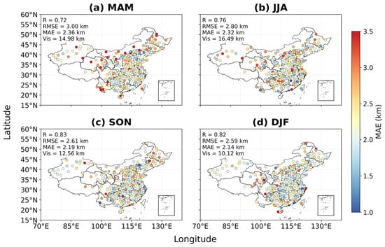
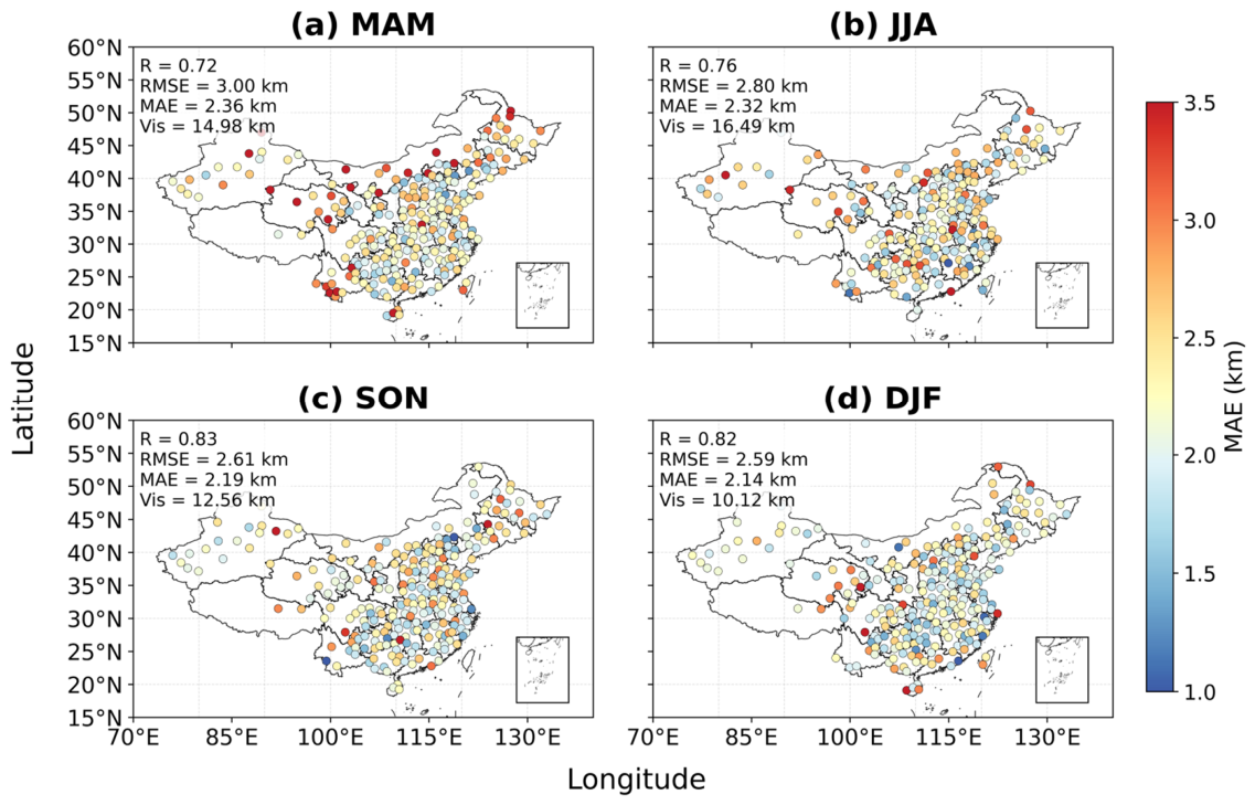
In addition to the overall and station-level validation results, the seasonal variation in visibility-estimation performance is presented in Figure 8. MAM represents March, April, and May; JJA represents June, July, and August; SON represents September, October, and November; and DJF represents December, January, and February. Among the four seasons, MAM exhibited the highest RMSE (3.00 km) and MAE (2.36 km), whereas DJF showed the lowest values (2.59 km and 2.14 km, respectively). The highest correlation was observed in SON (R = 0.83), followed by DJF (R = 0.82). Mean observed visibility also varied seasonally, reaching 16.49 km in JJA and 10.12 km in DJF.

Figure 8. Seasonal distributions of station-level mean absolute error (MAE) for Phy_RH_Res based on sample-based five-fold cross-validation out-of-fold predictions: (a) MAM (spring); (b) JJA (summer); (c) SON (autumn); and (d) DJF (winter). The overall R, RMSE, MAE, and mean observed visibility for the corresponding seasonal samples are shown in each panel.

Clear regional differences were also observed in the seasonal station-level MAE distributions. The locations and magnitudes of relatively large errors varied among seasons. Some western, northwestern, and northeastern stations exhibited relatively large MAE across multiple seasons, which is broadly consistent with the overall spatial RMSE and MAE patterns shown in Figure 7.

4.2.4. Model Component Ablation and Benchmark Comparison

To quantify the contribution of the main components of the proposed visibility estimation framework, five model configurations were compared: the basic physical estimate model (Phy_Base), the physical estimate with explicit relative-humidity adjustment (Phy_RH), the physical estimate followed by XGBoost residual correction without explicit RH adjustment (Phy_Res), and the complete framework incorporating both RH adjustment and residual learning (Phy_RH_Res). A direct XGBoost model (Direct_XGB) was additionally included as a benchmark. It used the same raw aerosol, meteorological, and temporal predictors to estimate visibility directly, without the physical estimate or residual-learning formulation. The corresponding performance metrics are summarized in Table 3.

Table 3. Performance comparison of the five model configurations using the model-development dataset (N = 16,234). Metrics for Phy_Res, Phy_RH_Res, and Direct_XGB are based on out-of-fold predictions from sample-based five-fold cross-validation.

Model	R	RMSE (km)	MAE (km)
Phy_Base	0.33	16.64	11.36
Phy_RH	0.36	15.97	10.41
Phy_Res	0.79	3.13	2.46
Phy_RH_Res	0.84	2.80	2.28
Direct_XGB	0.83	2.86	2.36

The standalone physical estimate (Phy_Base) showed poor estimation performance, with R = 0.33, RMSE = 16.64 km, and MAE = 11.36 km. Introducing the explicit RH adjustment alone (Phy_RH) resulted in a modest improvement, increasing R to 0.36 and reducing RMSE and MAE to 15.97 and 10.41 km, respectively. In contrast, introducing XGBoost-based residual correction (Phy_Res) substantially improved model performance, with R increasing to 0.79 and RMSE and MAE decreasing to 3.13 and 2.46 km, respectively. The complete framework (Phy_RH_Res) achieved R = 0.84, RMSE = 2.80 km, and MAE = 2.28 km.

These results show that the XGBoost residual-correction stage accounts for the largest improvement over the simplified physical estimate, whereas the explicit RH adjustment provides a smaller incremental improvement. The additional reduction in RMSE and MAE from Phy_Res to Phy_RH_Res further indicates that the RH-adjusted physical estimate contributes to the performance of the complete framework.

The comparison between Phy_RH_Res and Direct_XGB was further extended to the four cross-validation strategies (Table 4). Under sample-based cross-validation, Phy_RH_Res achieved a slightly lower RMSE than Direct_XGB (2.80 versus 2.86 km), with similarly modest improvements under day-based and site-based validation. In contrast, Direct_XGB obtained a slightly lower RMSE under month-based cross-validation (3.85 versus 3.90 km), while Phy_RH_Res retained a marginally lower MAE (3.08 versus 3.10 km). Overall, the two models exhibited comparable predictive performance, with small differences depending on the validation strategy. Their relative performance under different visibility conditions is further discussed in Section 5.2.

Table 4. Comparison of the performances of Direct_XGB and Phy_RH_Res under four five-fold cross-validation strategies using identical model-development samples and validation partitions.

Validation Strategy	Model	R	RMSE (km)	MAE (km)
Sample-based CV	Direct_XGB	0.83	2.86	2.36
	Phy_RH_Res	0.84	2.80	2.28
Day-based CV	Direct_XGB	0.82	2.91	2.41
	Phy_RH_Res	0.83	2.87	2.32
Month-based CV	Direct_XGB	0.68	3.85	3.10
	Phy_RH_Res	0.67	3.90	3.08
Site-based CV	Direct_XGB	0.82	2.91	2.39
	Phy_RH_Res	0.83	2.84	2.30

4.2.5. Evaluation of the Empirical RH-Conditioned Adjustment

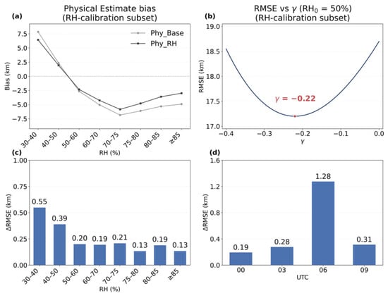
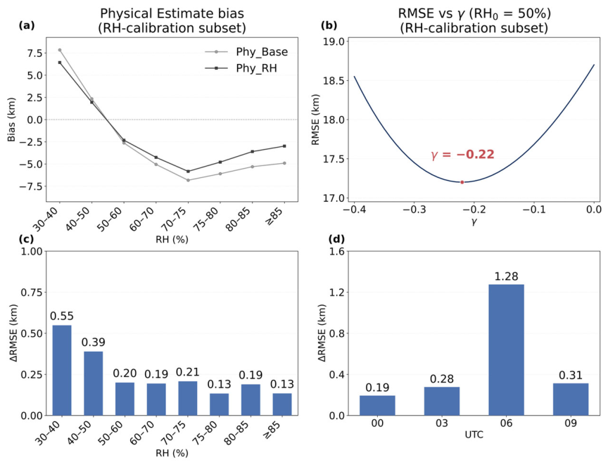
The empirical RH adjustment was further examined using the isolated RH-calibration subset. Figure 9a shows the variation in the mean bias of the first-order physical estimate (Phy_Base) across RH intervals. The bias decreased from positive values at lower RH to negative values at higher RH, with a transition near 50% RH. Accordingly, RH₀ = 50% was selected as the reference humidity for the normalized adjustment. For comparison, Figure 9a also shows the corresponding mean bias after applying the calibrated RH adjustment (Phy_RH). Compared with Phy_Base, Phy_RH exhibits smaller negative biases at higher RH, indicating that the adjustment partially alleviates the underestimation of visibility under high-RH conditions.

Figure 9. Calibration and evaluation of the empirical RH adjustment: (a) RH-dependent mean bias of Phy_Base and Phy_RH using the isolated RH-calibration subset; (b) sensitivity of calibration RMSE to γ with RH₀ fixed at 50%, using the same calibration subset; (c) RMSE reduction across RH intervals; and (d) RMSE reduction across UTC observation times. For panels (c,d), ΔRMSE is defined as RMSE(Phy_Res) − RMSE(Phy_RH_Res).

With RH₀ fixed at 50%, the sensitivity of calibration RMSE to γ was evaluated (Figure 9b). The RMSE varied with γ and reached a near-minimum level around the selected value of γ = −0.22. The resulting value of γ was subsequently held fixed for model training and evaluation.

The incremental improvement of the RH adjustment was then evaluated across RH intervals using out-of-fold predictions from sample-based five-fold cross-validation (Figure 9c). Compared with Phy_Res, Phy_RH_Res achieved lower RMSE across all evaluated RH intervals, with relatively larger reductions at the lower and higher ends of the evaluated RH range and smaller improvements over the mid-range RH intervals.

It was also evaluated across the four UTC observation times (Figure 9d). RMSE reductions were observed at all four time slots, ranging from 0.19 to 0.31 km at 00, 03, and 09 UTC. The largest reduction occurred at 06 UTC, where RMSE decreased from 4.95 to 3.68 km.

4.2.6. Independent Validation

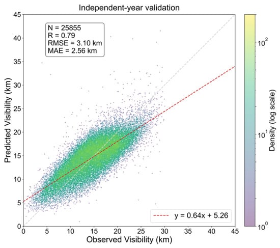
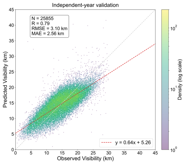
To further evaluate the robustness and generalization capability of the proposed visibility estimation framework on temporally independent data, an independent validation was conducted using observations from July 2024 to June 2025. The model was trained using the July 2023–June 2024 model-development subset and subsequently applied to the following 12-month period. A total of 25,855 independent matched samples were included in this evaluation.

As shown in Figure 10, the correlation coefficient R between the modelled and reference visibility is 0.79, the RMSE is 3.10 km and the MAE is 2.56 km. Visibility tends to be slightly overestimated at the lower end of the observed visibility range and underestimated at the higher end.

Figure 10. Independent-year validation from July 2024 to June 2025.

Table 5 further compares the independent-year performance of Phy_RH_Res and Direct_XGB. Phy_RH_Res achieved lower RMSE (3.10 versus 3.25 km) and MAE (2.56 versus 2.70 km) than Direct_XGB. Compared with the sample-based five-fold cross-validation results, the independent validation showed a moderate reduction in predictive performance. Moreover, compared with the sample-based cross-validation results, Phy_RH_Res exhibited a smaller increase in RMSE than Direct_XGB, suggesting a modest advantage of the physically informed framework in temporal generalization to an independent year.

Table 5. Overall performance comparison between Phy_RH_Res and Direct_XGB during the independent validation period (July 2024–June 2025).

Model	R	RMSE (km)	MAE (km)
Phy_RH_Res	0.79	3.10	2.56
Direct_XGB	0.77	3.25	2.70

4.3. Hourly Visibility Mapping Case Study

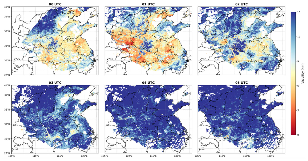
To demonstrate the spatial application of the developed model, hourly visibility maps at 4 km resolution were generated for a low-visibility event over the Chinese mainland. Figure 11 displays the successive estimated visibility fields from 00–05 UTC on 30 October 2024, illustrating the evolution of a morning low-visibility event. Between 00–01 UTC (8:00–9:00 local time), the maps showed extensive areas of low estimated visibility in Central and Southeast China, with the lowest visibility below 2 km (dark red). By 02 UTC, the visibility had substantially increased over most of the region, with visibility of approximately 5–6 km at the center. From 03 to 05 UTC, visibility further increased over much of the affected region and the spatial distribution became relatively stable. This case illustrates the potential of repeated FY-4B observations to depict diurnal variations in estimated surface visibility where valid AOD retrievals are available.

Figure 11. Hourly estimated visibility distributions over a region of central and eastern China from 00 to 05 UTC on 30 October 2024. Note that visibility estimates below 2 km are associated with relatively large uncertainties and should be interpreted with caution.

The spatial coverage of the visibility estimates also varied during the displayed period. A distinct arc-shaped missing-data region appears on the western side of the 00 UTC panel, while scattered blank areas are present in several other panels. Visibility estimates can only be generated when valid FY-4B AOD retrievals are available, resulting in data gaps for regions where the AOD retrieval is not successful. The causes and implications of these data gaps, together with the applicability and limitations of the optical-AOD-based visibility framework, are further discussed in Section 5.

5. Discussion

5.1. Model Performance and Generalization

The different cross-validation strategies reveal distinct constraints on model generalization. Relative to sample-based cross-validation, performance changed only modestly under day-based and site-based partitioning but declined more substantially when samples were separated by month. This greater sensitivity to monthly partitioning may be associated with temporal changes in the relationship between column-integrated AOD and surface visibility. Previous observations over China have shown that the temporal variations of column aerosol optical thickness and surface visibility do not necessarily correspond, partly because of differences in aerosol vertical distribution [29].

The station-level evaluation in Figure 7 shows regional differences in estimation errors. These differences may partly reflect variations in the relationship between column-integrated AOD, meteorological conditions, and local surface visibility. However, the present station-level evaluation cannot isolate the individual sources of these regional differences.

The diurnal differences in physical-estimate errors (Figure 6) highlight a limitation of applying a simplified AOD-to-visibility conversion across daytime observation times. The relationship between column-integrated AOD and near-surface extinction depends on aerosol vertical distribution, aerosol microphysical and optical properties and meteorological conditions, which can vary throughout the day and affect the accuracy of the simplified physical conversion. The FY-4B AOD validation (Table 2) showed relatively higher retrieval accuracy around 00 UTC and generally lower accuracy during subsequent daytime intervals. A broadly similar temporal pattern was observed in the physical-estimated visibility errors (Figure 6). In addition, relatively large visibility-estimation errors were observed at several stations in northwestern China and along the eastern coast (Figure 7). These spatial patterns are consistent with previously reported challenges in satellite AOD retrieval over bright, sparsely vegetated surfaces in northwestern China [30] and over heterogeneous coastal areas affected by mixed land–water pixels [31]. This suggests that AOD retrieval uncertainty may be one of the factors contributing to the observed differences in visibility-estimation errors. However, surface visibility is also influenced by aerosol vertical distribution, relative humidity, boundary-layer conditions, and other meteorological factors. Therefore, the individual contribution of AOD retrieval uncertainty to the final visibility-estimation errors cannot be quantitatively determined from the present results.

The independent-year evaluation further demonstrates the predictive value of the physically informed framework under temporally independent conditions. Compared with Direct_XGB, Phy_RH_Res achieved lower overall RMSE and MAE.

5.2. Roles of Model Components

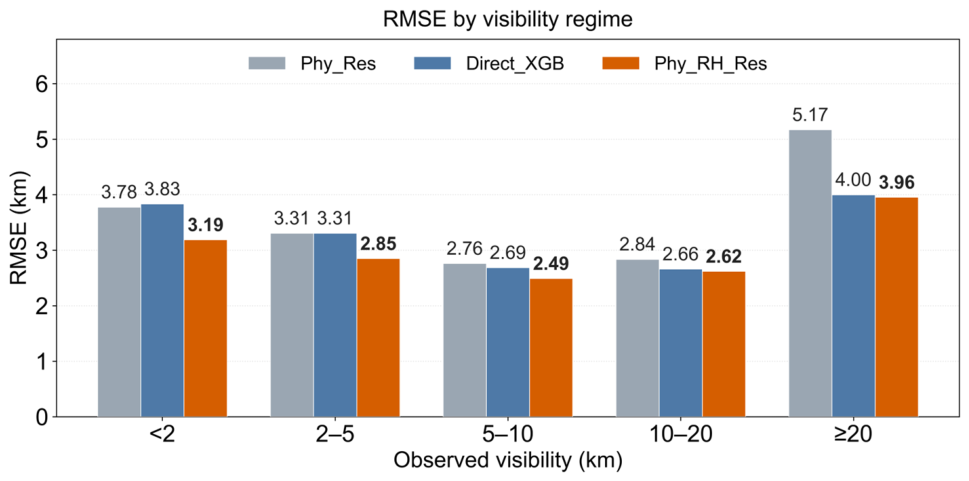
Figure 12 compares the RMSE of Phy_Res, Direct_XGB, and Phy_RH_Res across five observed-visibility intervals. As shown in the figure, Phy_RH_Res achieved the lowest RMSE among the three models in all five intervals. The empirical RH adjustment also showed lower RMSE across the evaluated RH intervals and four UTC observation times (Figure 9c,d). These findings support the incremental predictive value of the empirical adjustment within the present framework without implying a direct relationship between its performance gains and aerosol hygroscopic processes.

Figure 12. Visibility-stratified RMSE comparison among Phy_Res, Direct_XGB, and Phy_RH_Res across five observed-visibility intervals, based on sample-based five-fold cross-validation. Lower RMSE indicates better predictive performance.

Compared with Direct_XGB, Phy_RH_Res showed clearer predictive advantages under reduced-visibility conditions below 10 km (Figure 12). In particular, RMSE decreased from 3.83 to 3.19 km for visibility below 2 km and from 3.31 to 2.85 km for the 2–5 km interval. Furthermore, the independent-year validation (Table 5) showed lower overall RMSE and MAE for Phy_RH_Res than for Direct_XGB, supporting its advantage in temporal generalization.

5.3. Applicability and Practical Implications

Previous studies have established different approaches to large-scale surface visibility estimation. Table 6 compares the present study with representative previous studies in terms of observational inputs, spatiotemporal characteristics, and reported predictive performance.

Table 6. Comparison with representative studies on gridded surface visibility estimation.

Study	Main Inputs	Spatial and Temporal Resolution	Model Performance R/RMSE (km)	Independent-Year R/RMSE (km)
Zhang et al. [4]	Ground PM observations, CLDAS	China; seamless hourly; 6.25 km	0.95/3.17	0.85/5.28
He et al. [14]	MODIS AOD	Global; daily; 0.1°	0.85/2.70	—
This study	FY-4B AOD	China; multiple daytime observation times; ~4 km output grid	0.84/2.80	0.79/3.10

The comparison highlights different research objectives and observational approaches. Zhang et al. [4] developed seamless hourly visibility estimates over China driven by ground PM_2.5 observations and gridded meteorological data. While achieving continuous spatial coverage, this approach relies heavily on ground monitoring networks, with greater dependence on statistical extrapolation in regions with sparse observations. He et al. [14] advanced satellite-AOD-based visibility estimation to the global scale using MODIS observations and produced daily visibility maps. Building on these advances, the present study uses FY-4B AOD observations to evaluate visibility estimation at different daytime observation times. This extends the application of satellite AOD from predominantly daily-scale estimation toward diurnal visibility monitoring. However, the reported accuracy metrics across studies are not directly comparable because of differences in observational inputs and validation settings.

The successive visibility maps (Figure 11) further illustrate the application of repeated FY-4B observations to regional daytime visibility estimation. These maps provide a gridded perspective on estimated diurnal visibility variations, complementing ground-based station measurements where valid satellite AOD retrievals are available.

5.4. Limitations

As the proposed framework relies on satellite-retrieved AOD, its applicability is primarily limited to daytime, cloud-free conditions. Cloud cover, fog, and other unfavorable retrieval conditions may reduce the availability and reliability of AOD observations. Furthermore, uncertainties in satellite AOD can propagate into the initial visibility estimate, affecting the accuracy of the subsequent retrieval. In particular, the current framework is not suitable for reliably monitoring fog or very low-visibility conditions at or below 1–2 km, as indicated by the limited detection performance for these events.

The physical estimation also involves simplifications in representing aerosol vertical distribution. The assumption of an exponentially decreasing extinction profile, with PBLH used as an approximation of aerosol scale height, may be less appropriate in the presence of elevated aerosol layers, residual layers, or complex vertical stratification. Variations in aerosol composition and optical properties may introduce additional uncertainty into the relationship between column AOD and surface visibility. Although residual learning can reduce estimation errors, it does not independently resolve these physical uncertainties. In addition, the ERA5 meteorological fields were interpolated to the approximately 4 km FY-4B AOD grid, but their original 0.25° resolution may limit the representation of fine-scale meteorological variability. Improving the effective spatial detail of the estimates would therefore benefit from finer-resolution meteorological information.

The evaluation is also constrained by the characteristics of ground-based reference observations. Validation stations are unevenly distributed, and ground-based visibility measurements may be subject to upper measurement or reporting limits, affecting the representation of high-visibility conditions. In addition, the quantitative diurnal evaluation is based on four three-hourly observation times. Although the hourly FY-4B AOD and ERA5 inputs allow visibility estimates to be generated at intermediate hours, their prediction accuracy has not been independently evaluated at every daytime hour. Specifically, the estimates at 01, 02, 04, and 05 UTC in Figure 11 represent extrapolation to hour values not included in the model training data, and their prediction accuracy has not been independently verified.

6. Conclusions

This study investigated diurnal surface visibility estimation over China using FY-4B geostationary satellite AOD and a physically informed residual-learning framework. The complete model achieved R = 0.84, RMSE = 2.80 km, and MAE = 2.28 km under sample-based five-fold cross-validation. Independent validation using observations from July 2024 to June 2025 yielded R = 0.79, RMSE = 3.10 km, and MAE = 2.56 km, indicating reasonable predictive performance when applied to a subsequent observation year.

Visibility-estimation accuracy showed clear diurnal variations, with generally better performance at 00 and 03 UTC and the largest errors at 06 UTC. Errors at 09 UTC were also relatively low, although substantially fewer valid matched samples were available at this time slot. These time-dependent differences were evident in both the first-order physical estimate and the final model, indicating that variations in estimation accuracy persisted after RH adjustment and residual learning.

A systematic RH-dependent bias was also identified in the physical estimate, with visibility generally overestimated at lower RH and underestimated at higher RH, and a transition near 50%. The empirical RH adjustment was introduced to address this opposing bias pattern and reduced the overall RMSE of the physical estimate from 16.64 to 15.97 km. Controlled ablation experiments further showed that incorporating the RH-adjusted physical estimate reduced RMSE across all evaluated RH intervals and all four observation times, even though RH was already included as an XGBoost predictor. While residual learning contributed most of the overall accuracy improvement, the RH adjustment provided an additional empirical refinement. The complete framework also achieved the lowest RMSE among the three models across all five evaluated visibility intervals, with particularly clear advantages over direct XGBoost regression under visibility below 10 km.

The estimation accuracy varied across seasons and regions, with lower RMSE in winter than in spring and relatively larger station-level errors at several western, northeastern, and coastal locations. The independent-year validation also showed lower overall RMSE and MAE for the proposed framework than for direct XGBoost regression, supporting its temporal generalization to a subsequent observation year. The hourly visibility maps further illustrated the potential of repeated FY-4B AOD observations for characterizing regional diurnal variations in estimated visibility. Overall, these findings support the use of geostationary satellite AOD for quantitative daytime visibility estimation and underscore the importance of evaluating estimation accuracy across different observation times and regions.

References

- Horvath, H. Atmospheric Visibility. Atmos. Environ. 1981, 15, 1785–1796. [Google Scholar] [CrossRef] [Scilit]
- Qian, W.; Leung, J.C.-H.; Chen, Y.; Huang, S. Applying Anomaly-Based Weather Analysis to the Prediction of Low Visibility Associated with the Coastal Fog at Ningbo-Zhoushan Port in East China. Adv. Atmos. Sci. 2019, 36, 1060–1077. [Google Scholar] [CrossRef] [Scilit]
- Gultepe, I.; Sharman, R.; Williams, P.D.; Zhou, B.; Ellrod, G.; Minnis, P.; Trier, S.; Griffin, S.; Yum, S.S.; Gharabaghi, B.; et al. A Review of High Impact Weather for Aviation Meteorology. Pure Appl. Geophys. 2019, 176, 1869–1921. [Google Scholar] [CrossRef] [Scilit]
- Zhang, X.; Gui, K.; Zeng, Z.; Fei, Y.; Li, L.; Zheng, Y.; Peng, Y.; Liu, Y.; Shang, N.; Zhao, H.; et al. Mapping the Seamless Hourly Surface Visibility in China: A Real-Time Retrieval Framework Using a Machine-Learning-Based Stacked Ensemble Model. npj Clim. Atmos. Sci. 2024, 7, 68. [Google Scholar] [CrossRef] [Scilit]
- Shahzad, M.I.; Nichol, J.E.; Wang, J.; Campbell, J.R.; Chan, P.W. Estimating Surface Visibility at Hong Kong from Ground-Based LIDAR, Sun Photometer and Operational MODIS Products. J. Air Waste Manag. Assoc. 2013, 63, 1098–1110. [Google Scholar] [CrossRef] [Scilit] [PubMed]
- Koschmieder, H. Theorie Der Horizontalen Sichtweite. Beitr. Phys. Freien Atmos. 1924, 12, 33–53. [Google Scholar]
- Malm, W.C.; Sisler, J.F.; Huffman, D.; Eldred, R.A.; Cahill, T.A. Spatial and Seasonal Trends in Particle Concentration and Optical Extinction in the United States. J. Geophys. Res. Atmos. 1994, 99, 1347–1370. [Google Scholar] [CrossRef] [Scilit]
- Li, Z.; Gu, X.; Wang, L.; Li, D.; Xie, Y.; Li, K.; Dubovik, O.; Schuster, G.; Goloub, P.; Zhang, Y.; et al. Aerosol Physical and Chemical Properties Retrieved from Ground-Based Remote Sensing Measurements during Heavy Haze Days in Beijing Winter. Atmos. Chem. Phys. 2013, 13, 10171–10183. [Google Scholar] [CrossRef] [Scilit]
- Retalis, A.; Hadjimitsis, D.G.; Michaelides, S.; Tymvios, F.; Chrysoulakis, N.; Clayton, C.R.I.; Themistocleous, K. Comparison of Aerosol Optical Thickness with in Situ Visibility Data over Cyprus. Nat. Hazards Earth Syst. Sci. 2010, 10, 421–428. [Google Scholar] [CrossRef] [Scilit]
- Kessner, A.L.; Wang, J.; Levy, R.C.; Colarco, P.R. Remote Sensing of Surface Visibility from Space: A Look at the United States East Coast. Atmos. Environ. 2013, 81, 136–147. [Google Scholar] [CrossRef] [Scilit]
- Lee, K.H.; Wong, M.S.; Kim, K.; Park, S.S. Analytical Approach to Estimating Aerosol Extinction and Visibility from Satellite Observations. Atmos. Environ. 2014, 91, 127–136. [Google Scholar] [CrossRef] [Scilit]
- Shang, N.; Gui, K.; Cheng, T.; Zhao, H.; Zhang, X.; Yao, W.; Zheng, Y.; Li, L.; Liu, Y.; Wang, H.; et al. Factors Influencing the Relationships between Hourly Visibility and Aerosol Optical Depth in China—Implications for Hourly Aerosol Optical Depth Retrievals Using Automatic Visibility Observations. Atmos. Environ. 2025, 358, 121353. [Google Scholar] [CrossRef] [Scilit]
- Shan, Y.; Zhang, R.; Gultepe, I.; Zhang, Y.; Li, M.; Wang, Y. Gridded Visibility Products over Marine Environments Based on Artificial Neural Network Analysis. Appl. Sci. 2019, 9, 4487. [Google Scholar] [CrossRef] [Scilit]
- He, J.; Wang, W.; Fu, M.; Wang, Y. Insights into Global Visibility Patterns: Spatiotemporal Distributions Revealed by Satellite Remote Sensing. J. Clean. Prod. 2024, 468, 143069. [Google Scholar] [CrossRef] [Scilit]
- Zieger, P.; Fierz-Schmidhauser, R.; Weingartner, E.; Baltensperger, U. Effects of Relative Humidity on Aerosol Light Scattering: Results from Different European Sites. Atmos. Chem. Phys. 2013, 13, 10609–10631. [Google Scholar] [CrossRef] [Scilit]
- Brunner, J.; Pierce, R.B.; Lenzen, A. Development and Validation of Satellite-Based Estimates of Surface Visibility. Atmos. Meas. Tech. 2016, 9, 409–422. [Google Scholar] [CrossRef] [Scilit]
- Holben, B.N.; Eck, T.F.; Slutsker, I.; Tanré, D.; Buis, J.P.; Setzer, A.; Vermote, E.; Reagan, J.A.; Kaufman, Y.J.; Nakajima, T.; et al. AERONET—A Federated Instrument Network and Data Archive for Aerosol Characterization. Remote Sens. Environ. 1998, 66, 1–16. [Google Scholar] [CrossRef] [Scilit]
- Zhou, D.; Wang, Q.; Li, S.; Yang, J. Preliminary Retrieval and Validation of Aerosol Optical Depths from FY-4B Advanced Geostationary Radiation Imager Images. Remote Sens. 2024, 16, 372. [Google Scholar] [CrossRef] [Scilit]
- Si, Y.; Wang, L.; Chen, L.; Cheng, Y.; Dai, T.; Gao, L.; Zhang, X.; Li, B.; Zhang, X.; Lu, F. Coupling Hourly Land Surface Models With Spatiotemporal Variability Characteristics: A Study on FY-4B/AGRI Land Aerosol Retrieval Algorithm. IEEE Trans. Geosci. Remote Sens. 2025, 63, 1–20. [Google Scholar] [CrossRef] [Scilit]
- Ångström, A. On the Atmospheric Transmission of Sun Radiation and on Dust in the Air. Geogr. Ann. 1929, 11, 156–166. [Google Scholar] [CrossRef] [Scilit]
- Wei, G.; Wang, S.; Gao, Z.; Liu, B.; Zha, Y. Influences of Meteorological Factors on Aerosol Optical Depth and Near-Surface Aerosol Extinction Coefficient. J. Indian Soc. Remote Sens. 2025, 53, 4281–4296. [Google Scholar] [CrossRef] [Scilit]
- Gultepe, I.; Tardif, R.; Michaelides, S.C.; Cermak, J.; Bott, A.; Bendix, J.; Müller, M.D.; Pagowski, M.; Hansen, B.; Ellrod, G.; et al. Fog Research: A Review of Past Achievements and Future Perspectives. Pure Appl. Geophys. 2007, 164, 1121–1159. [Google Scholar] [CrossRef] [Scilit]
- Singh, A.; Bloss, W.J.; Pope, F.D. 60 Years of UK Visibility Measurements: Impact of Meteorology and Atmospheric Pollutants on Visibility. Atmos. Chem. Phys. 2017, 17, 2085–2101. [Google Scholar] [CrossRef] [Scilit]
- Smith, A.; Lott, N.; Vose, R. The Integrated Surface Database: Recent Developments and Partnerships. Bull. Am. Meteorol. Soc. 2011, 92, 704–708. [Google Scholar] [CrossRef] [Scilit]
- Koelemeijer, R.B.A.; Homan, C.D.; Matthijsen, J. Comparison of Spatial and Temporal Variations of Aerosol Optical Thickness and Particulate Matter over Europe. Atmos. Environ. 2006, 40, 5304–5315. [Google Scholar] [CrossRef] [Scilit]
- Zeng, Q.; Chen, L.; Zhu, H.; Wang, Z.; Wang, X.; Zhang, L.; Gu, T.; Zhu, G.; Zhang, Y. Satellite-Based Estimation of Hourly PM2.5 Concentrations Using a Vertical-Humidity Correction Method from Himawari-AOD in Hebei. Sensors 2018, 18, 3456. [Google Scholar] [CrossRef] [Scilit] [PubMed]
- Kasten, F. Visibility Forecast in the Phase of Pre-Condensation. Tellus Dyn. Meteorol. Oceanogr. 1969, 21, 631. [Google Scholar] [CrossRef] [Scilit]
- Chen, T.; Guestrin, C. XGBoost: A Scalable Tree Boosting System. In Proceedings of the 22nd ACM SIGKDD International Conference on Knowledge Discovery and Data Mining; ACM: San Francisco, CA, USA, 2016; pp. 785–794. [Google Scholar]
- Zhang, Z.Y.; Wong, M.S.; Lee, K.H. Evaluation of the Representativeness of Ground-Based Visibility for Analysing the Spatial and Temporal Variability of Aerosol Optical Thickness in China. Atmos. Environ. 2016, 147, 31–45. [Google Scholar] [CrossRef] [Scilit]
- Tao, M.; Chen, L.; Wang, Z.; Tao, J.; Che, H.; Wang, X.; Wang, Y. Comparison and Evaluation of the MODIS Collection 6 Aerosol Data in China. J. Geophys. Res. Atmos. 2015, 120, 6992–7005. [Google Scholar] [CrossRef] [Scilit]
- Remer, L.A.; Kaufman, Y.J.; Tanré, D.; Mattoo, S.; Chu, D.A.; Martins, J.V.; Li, R.-R.; Ichoku, C.; Levy, R.C.; Kleidman, R.G.; et al. The MODIS Aerosol Algorithm, Products, and Validation. J. Atmos. Sci. 2005, 62, 947–973. [Google Scholar] [CrossRef] [Scilit]
Disclaimer/Publisher’s Note: The statements, opinions and data contained in all publications are solely those of the individual author(s) and contributor(s) and not of MDPI and/or the editor(s). MDPI and/or the editor(s) disclaim responsibility for any injury to people or property resulting from any ideas, methods, instructions or products referred to in the content. |
© 2026 by the authors. Licensee MDPI, Basel, Switzerland. This article is an open access article distributed under the terms and conditions of the Creative Commons Attribution (CC BY) license.