A Lightweight Spectral–Spatial Network for Efficient Semantic Segmentation of Ground-Based Hyperspectral Imagery

Highlights

What are the main findings?

• A lightweight spectral-spatial network integrates spectral tokenization, coordinateselective feature mixing, and guided decoding for ground-based hyperspectral semantic segmentation.
• Experiments on HyKo2 and HSI-Drive demonstrate a favorable balance between segmentation accuracy, model size, and inference speed.

What are the implications of the main findings?

• The results support retaining full hyperspectral observations and learning compact spectral representations within the network for effective segmentation.
• Combining compact spectral encoding with directional context and adaptive localscale processing provides an efficient design for ground-based hyperspectral scene understanding.

Abstract

Ground-based hyperspectral imaging extends remote sensing to road environments by providing material-sensitive spectra for distinguishing visually similar surfaces and objects. However, pixel-wise prediction from high-dimensional spectral cubes is computationally demanding. This study presents a lightweight spectral–spatial network for efficient semantic segmentation of ground-based hyperspectral imagery. A Spectral Token Stem compresses ordered bands into pooled, normalized, and statistical descriptors before high-resolution encoding. CoordSK blocks combine coordinate-aware directional aggregation with adaptive local-scale selection, while a lightweight guided decoder recovers dense predictions from multi-level features. Experiments on the public HyKo2 and HSI-Drive datasets yield Jaccard indices of 0.6670 and 0.8181, respectively, outperforming representative efficient segmentation baselines. The model contains 0.656 million trainable parameters and reaches FP32 batch-one throughputs of 151.49 and 168.21 FPS on an RTX 5090 for the respective benchmarks. In the additional pretrained-model comparison, the network uses less than 0.5% of HSI-Adapter’s total parameters. Ablation studies validate the contributions of spectral tokenization and coordinate-selective mixing, and an input-representation study demonstrates the benefit of retaining full hyperspectral observations over PCA and pseudo-RGB inputs. These results indicate a favorable accuracy–efficiency trade-off for ground-based hyperspectral remote sensing scene understanding.

1. Introduction

Hyperspectral imaging is an important remote sensing modality because its contiguous spectral measurements reveal material properties that are not available from conventional RGB observations. Although hyperspectral remote sensing is often associated with airborne and spaceborne platforms, ground-based sensors can bring the same material-sensitive information to road environments, where visually similar surfaces or objects may have different spectral responses. This richer observation is computationally expensive: semantic segmentation must process a high-dimensional spectrum at every pixel, making arithmetic cost, model size, and realized throughput central design constraints for timely scene understanding.

Existing efficient semantic segmentation networks are mainly designed for RGB images. For example, BiSeNetV2 accelerates segmentation with separate detail and semantic branches plus guided aggregation [1], while DDRNet keeps parallel high- and low-resolution representations for efficient road-scene parsing [2]. These designs are effective for RGB dense prediction, but their architectures usually treat the input as a small set of visual channels and do not explicitly exploit the ordered spectral structure of hyperspectral observations. Directly applying them to hyperspectral cubes may therefore underuse the material-sensitive evidence carried by contiguous bands.

Recent hyperspectral semantic segmentation algorithms have begun to model spectral information more explicitly. UM2Former strengthens mixed spectral–spatial representation for large-scale hyperspectral segmentation [3], HSI-Adapter introduces adapter-based interaction between hyperspectral features and vision foundation models [4], and MSAM enhances U-Net with multi-scale spectral attention [5]. These methods improve hyperspectral representation learning, but many rely on relatively heavy backbones or feature-interaction designs. Ground-based hyperspectral remote sensing requires both accurate spectral–spatial modeling and an architecture that allocates computation selectively across high-resolution features.

To address these limitations, we propose a lightweight spectral–spatial network for efficient semantic segmentation of ground-based hyperspectral imagery. The network first uses a Spectral Token Stem to transform the raw hyperspectral cube into compact spectral–spatial features before high-resolution encoding. It then stacks CoordSK blocks to perform efficient feature mixing by combining coordinate-aware directional aggregation with adaptive local-scale selection. A lightweight guided decoder further fuses multi-level encoder features and restores dense predictions with limited computational overhead. This design treats hyperspectral scene understanding as a high-dimensional remote sensing problem in which spectral compression, spatial mixing, and decoder reconstruction must be balanced jointly.

The main contributions of this paper are summarized as follows:

• We design a compact Spectral Token Stem that reduces spectral redundancy at the network entrance while preserving material-sensitive cues in ground-based hyperspectral observations.
• We introduce the CoordSK block as an efficient spectral–spatial feature mixer that combines directional context with adaptive local receptive fields.
• We build a lightweight encoder–decoder framework and evaluate it on the public HyKo2 and HSI-Drive scene-understanding benchmarks in terms of pixel-wise segmentation accuracy, parameter count, FLOPs, and throughput, demonstrating a favorable accuracy–efficiency balance for ground-based hyperspectral remote sensing.

2. Related Work

2.1. Real-Time Semantic Segmentation

Real-time semantic segmentation focuses on dense prediction under strict latency and computation budgets. Yu et al. proposed BiSeNetV2, which separates detail and semantic branches and uses guided aggregation for efficient fusion [1]. Fan et al. proposed STDC to build a compact single-stream network through short-term dense concatenation [6]. Hong et al. developed DDRNet to maintain high- and low-resolution representations in parallel for road-scene segmentation [2]. Xu et al. proposed PIDNet, which uses proportional, integral, and derivative branches to strengthen detail, context, and boundary responses [7]. Meng et al. further introduced DMBR-Net to improve feature exchange across multiple resolutions [8]. These methods show that careful allocation of high-resolution and low-resolution computation is important for real-time segmentation.

Recent real-time segmentation methods also explore more efficient context modeling. Xu et al. proposed LETNet by combining efficient transformer-style modeling with CNN operators [9]. Zhengze Xu et al. proposed SCTNet to inject transformer semantic information into a single-branch CNN [10]. Gu et al. proposed RTLinearFormer to reduce attention cost with lightweight linear attention [11], while Lei et al. designed DSARFormer with dynamic sparse axial rectangular attention [12]. Wang et al. introduced LCS4 to use linear-complexity state-space modeling for efficient semantic segmentation [13]. Although these methods provide useful designs for efficient spatial modeling, they are mainly developed for RGB or multimodal inputs and do not explicitly preserve ordered spectral evidence from raw hyperspectral data.

2.2. Hyperspectral Remote Sensing Segmentation

Hyperspectral remote sensing segmentation must jointly handle dense spatial prediction and high-dimensional spectral responses. Gutierrez-Zaballa et al. explored fully convolutional networks for hyperspectral segmentation in advanced driver assistance systems and showed the importance of spatial convolution for real road scenes [14]. They further developed an on-chip FCN system for hyperspectral scene understanding, including preprocessing, embedded deployment, latency, and energy evaluation [15]. Shah et al. benchmarked standard semantic segmentation models for autonomous-driving hyperspectral perception [16], and Theisen et al. proposed HS3-Bench with unified evaluation protocols and strong baselines for driving-scenario hyperspectral segmentation [17]. These studies extend hyperspectral remote sensing from overhead observation to ground-level scene understanding, but many adopted networks remain adaptations of RGB segmentation backbones.

Recent works have introduced more explicit spectral modeling for hyperspectral segmentation. Hong et al. proposed SpectralFormer to model spectral relations with transformers [18]. Xu et al. proposed UM2Former, a U-shaped multimixed transformer network for large-scale hyperspectral semantic segmentation [3]. Shah et al. proposed MSAM to insert multi-scale spectral attention into U-Net skip connections for driving-scene hyperspectral segmentation [5]. Wang and Miyazaki proposed MobileSACNet, which uses lightweight spectral–spatial compression for autonomous-driving hyperspectral segmentation [19]. Hurtado et al. proposed HSI-Adapter to connect hyperspectral features with frozen vision foundation models through adapter-based interaction [4]. Shah et al. further proposed learnable quantum-efficiency filters to study trainable spectral responses from a sensor-design perspective [20]. These methods confirm the importance of spectral compression and spectral–spatial alignment, but many rely on U-shaped backbones, foundation-model priors, or sensor-level objectives. In contrast, our method combines early spectral tokenization, CoordSK-based high-resolution feature mixing, and lightweight guided decoding in a compact architecture for raw ground-based hyperspectral imagery.

Attention and feature interaction are also studied in related remote sensing tasks. Yang et al. developed an intra- and cross-scale interaction network that combines within-stage refinement with hierarchical feature integration for language-conditioned segmentation [21]. Their Spatial-Semantic Alignment and Change-Aware Network combines CNN spatial features with CLIP semantics for change captioning [22]. It further calibrates features using temporal differences and models spatial changes through multiple state-space paths.

For road extraction, TransRoadNet combines position attention, context extraction, and foreground-context supplementation at decoder stages [23]. The semantic–spatial refinement network CRNet uses deeper features to refine shallower representations through channel and spatial interactions before decoder fusion [24]. These works connect contextual feature refinement with cross-scale integration for dense scene understanding.

3. Proposed Method

3.1. Network Overview

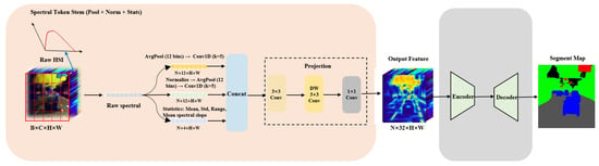
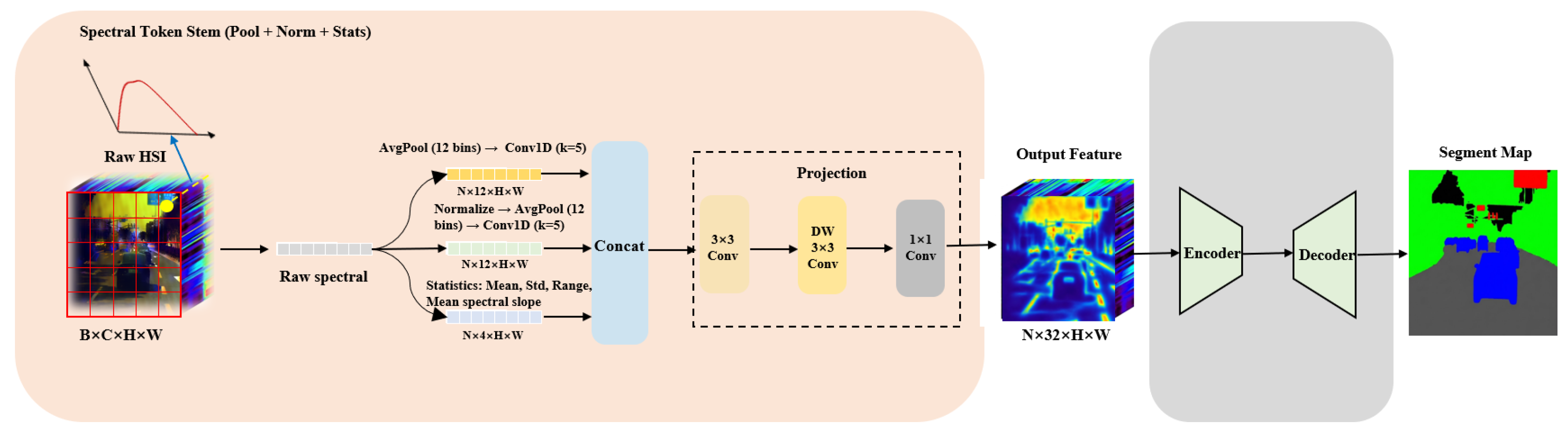
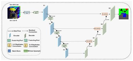
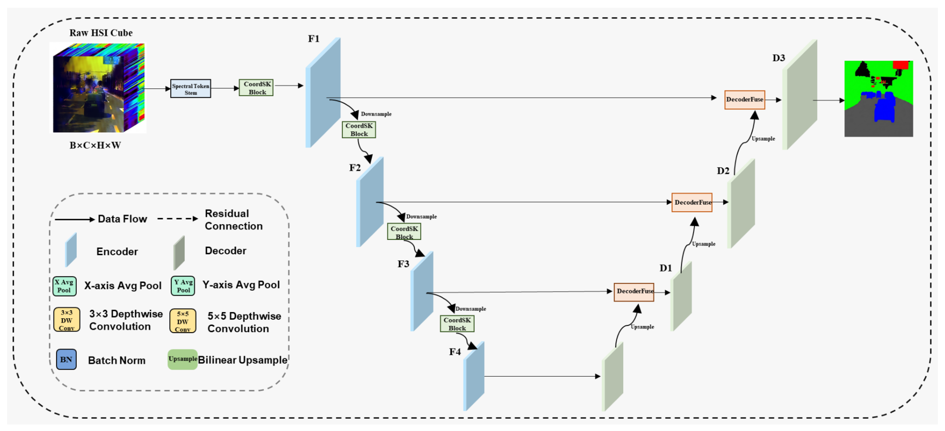
The proposed network is a compact encoder–decoder architecture that follows the data flow shown in Figure 1. Given a raw hyperspectral cube $X\in {\mathbb{R}}^{N\times C\times H\times W}$, where N is batch size and C is the number of spectral bands, the network first uses a Spectral Token Stem to convert the ordered spectral bands into a compact shallow feature map. This feature is processed by the encoder–decoder path, which is expanded in Figure 2. The encoder first produces $F_1$ with a CoordSK block and then repeats a downsampling-and-mixing pattern to obtain $F_2$, $F_3$, and $F_4$, where each stage uses CoordSK blocks for spatial–spectral feature mixing at its own resolution.

Figure 1. Main overview of the proposed network. The Spectral Token Stem combines pooled raw spectra, pooled normalized spectra, and four statistical descriptors (mean, standard deviation, range, and mean spectral slope). In the two pooling branches, AvgPool denotes 12-bin adaptive average pooling and Conv1D denotes spectral smoothing with kernel size 5. The concatenated descriptors are projected into a 32-channel feature map. The input batch dimension B in the diagram corresponds to N in the text. The resulting feature is then processed by the lightweight encoder–decoder path, expanded in Figure 2, to produce the semantic segmentation map. The peach and gray shaded regions denote the Spectral Token Stem and encoder–decoder path, respectively; arrows indicate data flow, and feature cubes represent intermediate tensors.

Figure 2. Detailed encoder–decoder expansion of the encoder and decoder blocks in Figure 1. The encoder extracts multi-resolution features using CoordSK blocks, and the decoder progressively restores dense predictions with skip-guided DecoderFuse units.

The decoder reconstructs dense predictions through three progressive fusion stages, denoted as $D_1$, $D_2$, and $D_3$ in Figure 2. Starting from the deepest encoder feature, the decoder upsamples the low-resolution representation and fuses it with the corresponding shallower feature through a DecoderFuse unit. Specifically, $F_4$ is decoded and fused with $F_3$ to form $D_1$, $D_1$ is fused with $F_2$ to form $D_2$, and $D_2$ is fused with $F_1$ to form $D_3$. A final prediction head maps $D_3$ to the segmentation mask. This layout places spectral compression before wide feature maps, uses coordinate-selective mixing inside the encoder stages, and keeps reconstruction shallow through guided skip fusion. The Spectral Token Stem is illustrated in Figure 1, and detailed diagrams of the CoordSK block and DecoderFuse module are shown in Figure 3 and Figure 4.

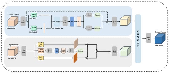
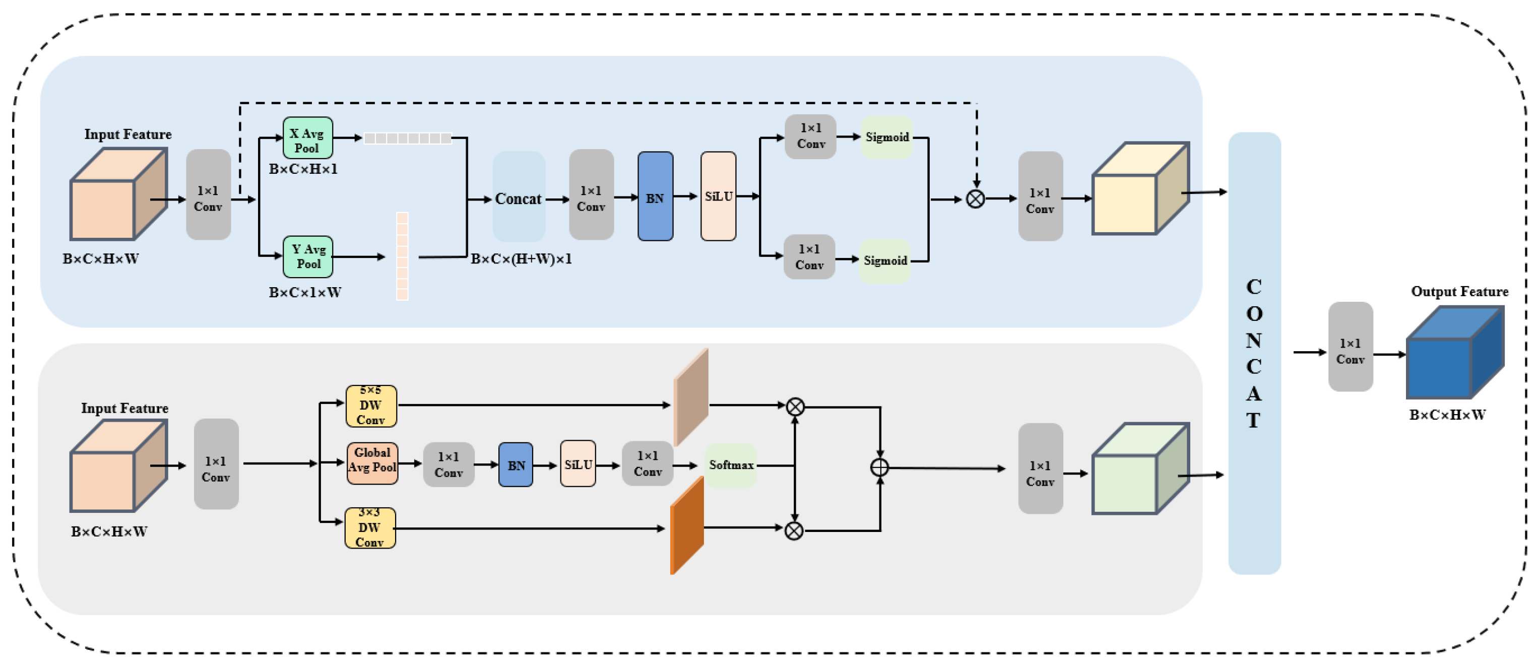
Figure 3. CoordSK block. The upper branch performs coordinate-aware directional aggregation with horizontal and vertical pooling, while the lower branch selects between lightweight local receptive fields. The branch outputs are concatenated, projected, residually scaled, and added to the input feature. The blue and gray shaded regions distinguish the coordinate and selective-kernel branches, respectively. Arrows indicate feature or modulation flow; circled multiplication and plus symbols denote element-wise multiplication and addition. The batch dimension B in the diagram corresponds to N in the equations.

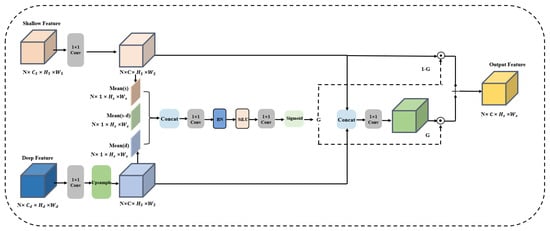
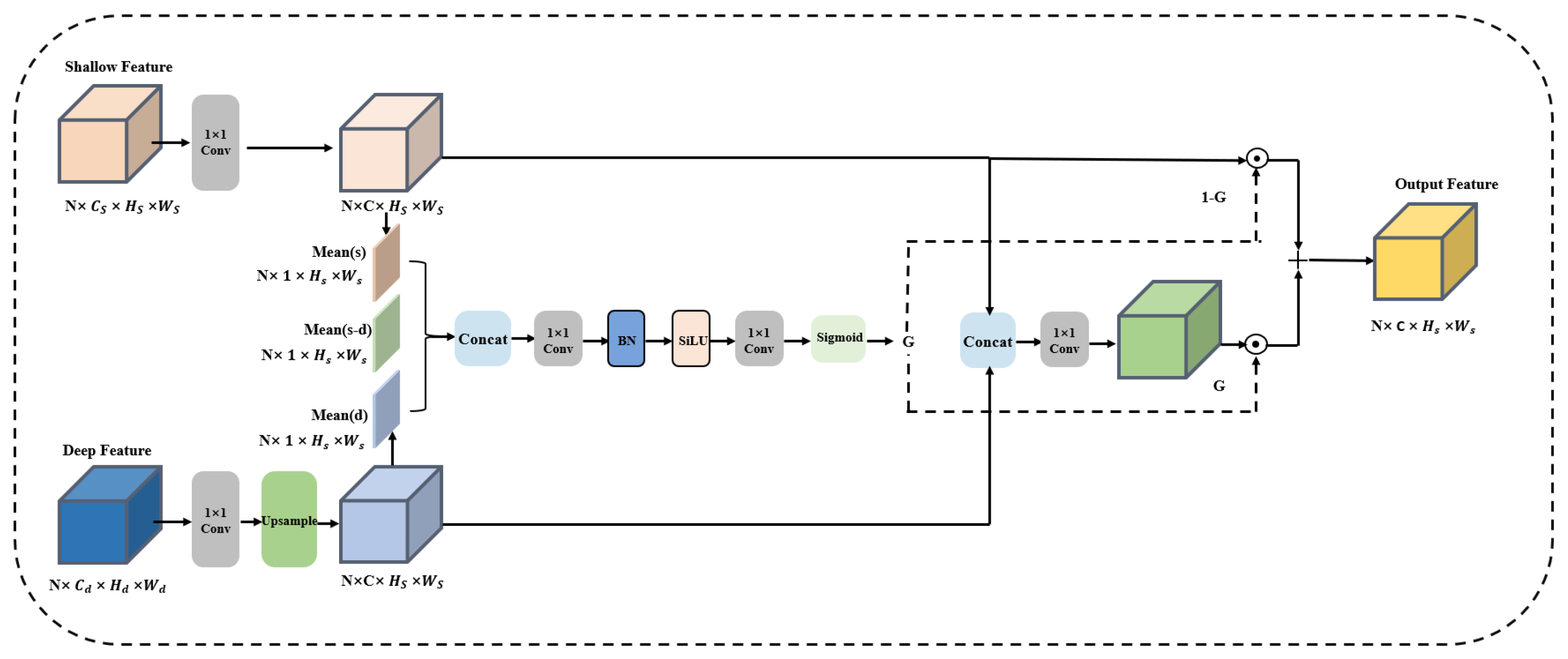
Figure 4. DecoderFuse module. The shallow and deep features are first channel-aligned, the deep feature is upsampled to the shallow resolution, and spectral–spatial summary cues are used to generate a gate for guided feature fusion. Solid arrows indicate feature flow, and dashed arrows carry the gate weights. Circled dot symbols denote element-wise multiplication, and the plus sign denotes addition.

3.2. Spectral Token Stem

The Spectral Token Stem illustrated in Figure 1 converts each raw per-pixel spectrum into a small set of structured descriptors before spatial encoding starts. For an input cube $X\in {\mathbb{R}}^{N\times C\times H\times W}$, the stem reads the spectral vector at each spatial location and builds three descriptor groups. The first group applies one-dimensional adaptive average pooling to each pixel spectrum, preserving spatial resolution. A shared one-dimensional convolution of kernel size 5 then smooths the pooled tokens. The second group applies the same operations to a normalized spectrum, reducing sample-dependent scale variation. The third group extracts simple statistical descriptors, including mean, standard deviation, range, and average spectral slope. In the default configuration, the pooled and normalized descriptors each contain 12 bins, while the statistics branch contains four channels.

$$T=\left[P_{12}\right(X);P_{12}(\widehat{X});\mathrm{Stats}(X\left)\right],$$

(1)

where $P_{12}(·)$ denotes 12-bin adaptive average pooling and spectral smoothing, $\widehat{X}$ is the normalized spectrum, and $[·;·]$ denotes channel concatenation. The concatenated descriptor tensor T is then passed through a lightweight projection stack consisting of a $3\times 3$ convolution, a $3\times 3$ depthwise convolution, and a $1\times 1$ projection. This produces the initial feature map

$$F_0=\Phi \left(T\right)\in {\mathbb{R}}^{N\times 32\times H\times W}.$$

(2)

The compact descriptor design preserves ordered spectral information while reducing the number of channels processed by subsequent high-resolution convolutions. Unless otherwise stated, the stem uses 12 pooled spectral bins; Section 4 further studies this bin count.

3.3. Coordinate-Selective Mixing Block

The CoordSK block in Figure 3 is the main encoder operator used after the spectral stem and after each downsampling stage. Given an input feature $U\in {\mathbb{R}}^{N\times C\times H\times W}$, the block first applies channel projection and then processes the feature with two complementary lightweight branches. The upper branch performs coordinate-aware directional aggregation. It computes average-pooled descriptors along the horizontal and vertical axes; concatenates the two directional descriptors; and uses $1\times 1$ convolutions, batch normalization, SiLU activation, and sigmoid gates to generate axis-aware modulation weights. This branch is used to preserve elongated spatial structures such as roads, lanes, and object boundaries.

The lower branch performs selective local scale mixing. It projects the input feature and sends it to lightweight depthwise convolutional paths, including $3\times 3$ and $5\times 5$ receptive fields. A compact global routing path generates soft selection weights, allowing the block to emphasize the receptive field that is more suitable for the current feature. Let $B_c(·)$ denote the coordinate branch and $B_s(·)$ denote the selective-kernel branch after channel alignment, so their outputs have the same shape as U. The two branch outputs are concatenated and projected as

$$Y=U+\beta \Pi \left(\left[B_c\right(U)-U;B_s(U)-U]\right),$$

(3)

where $[·;·]$ denotes channel concatenation, $\Pi (·)$ is a $1\times 1$ fusion projection, and $\beta$ is a learned residual scaling parameter. Each channel has its own residual scale, initialized to 0.04 and learned during training. The residual formulation combines directional context and adaptive local scale selection without introducing global attention.

The role of CoordSK in an efficient inference pipeline is therefore twofold. The coordinate branch provides long horizontal and vertical context with pooling-based operations, while the selective-kernel branch adapts local receptive fields using depthwise convolutions. This matches the encoder layout in Figure 1, where CoordSK is repeatedly used at high and medium resolutions and efficient operators are required for single-sample inference.

3.4. Lightweight Decoder

The DecoderFuse module in Figure 4 defines how each decoder stage combines a shallow encoder feature with a deeper semantic feature. Let $S\in {\mathbb{R}}^{N\times C_s\times H_s\times W_s}$ be the shallow feature from the encoder skip connection, and let $D\in {\mathbb{R}}^{N\times C_d\times H_d\times W_d}$ be the deeper decoder feature. DecoderFuse first applies $1\times 1$ convolutions to align the channel dimensions and upsamples the deep feature to the shallow resolution, giving $\overline{S},\tilde{D}\in {\mathbb{R}}^{N\times C\times H_s\times W_s}$. Let $s=\overline{S}$ and $d=\tilde{D}$ denote these aligned features.

After alignment, DecoderFuse builds a small guidance signal from the shallow feature, the upsampled deep feature, and their difference. As shown in Figure 4, the module computes summary maps from s, $s-d$, and d, concatenates these cues, and passes them through a lightweight $1\times 1$ convolutional gate. The summary tensor and gate are written as

$$Q=\left[\mathrm{Mean}\right(s);\mathrm{Mean}(s-d);\mathrm{Mean}(d\left)\right],$$

(4)

$$G=\sigma (\Psi \left(Q\right)),O=(1-G)\odot \overline{S}+G\odot \Theta \left([\overline{S};\tilde{D}]\right),$$

(5)

where $\Psi (·)$ and $\Theta (·)$ are lightweight $1\times 1$ projections and ⊙ denotes element-wise multiplication. This guided fusion is applied progressively from deep to shallow features: $F_4$ with $F_3$, then $D_1$ with $F_2$, and finally $D_2$ with $F_1$. The decoder remains shallow, so most computation stays in the spectral stem and CoordSK encoder while the output path preserves high-resolution detail through skip-guided fusion.

4. Experimental Results and Discussion

4.1. Datasets and Evaluation Metrics

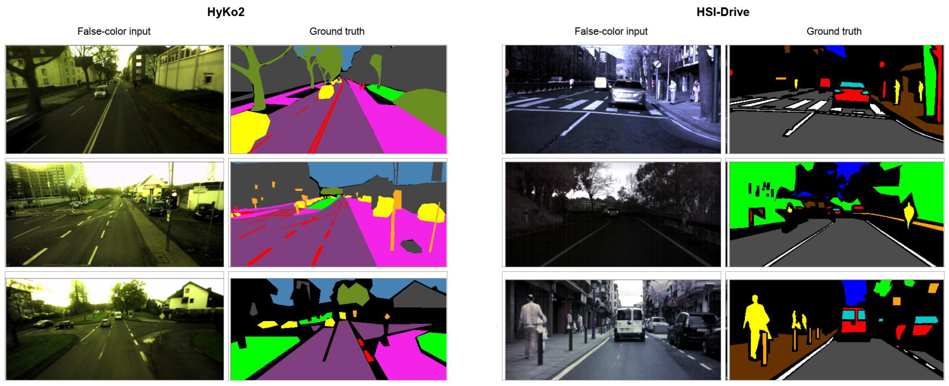
We evaluate the proposed network on two ground-based hyperspectral semantic segmentation datasets, HyKo2 and HSI-Drive, under the raw-hyperspectral protocol used in HS3-Bench [17]. Figure 5 shows representative false-color inputs and semantic annotations from the two datasets. The benchmarks are complementary: HyKo2 provides compact urban scenes with fine semantic structure, whereas HSI-Drive provides larger driving scenes with outdoor illumination, material, and viewpoint variability.

Figure 5. Representative dataset examples used in the experiments. Left: HyKo2 scenes. Right: HSI-Drive scenes. Each panel shows false-color hyperspectral visualization and the corresponding semantic ground truth. HyKo2 semantic colors are purple for road, magenta for sidewalk, red for lane markers, bright green for grass, olive for vegetation, orange for panels/signs/traffic lights, gray for buildings, yellow for vehicles, crimson for persons, and steel blue for sky. HSI-Drive colors are dark gray for road, white for road marks, green for vegetation, red for painted metal, blue for sky, brown for concrete/stone/brick, yellow for pedestrians/cyclists, orange for unpainted metal, and cyan for glass/transparent plastic. Black denotes undefined labels in these examples.

HyKo2 is used as a compact ground-level hyperspectral segmentation benchmark. In our protocol, each sample is represented by 15 spectral channels and is evaluated with the semantic label definition containing road, sidewalk, lane markers, grass, vegetation, traffic panels/signs/lights, buildings, vehicles, pedestrians, sky, and undefined regions. The split contains 81 training samples, 32 validation samples, and 49 test samples. HyKo2 emphasizes fine urban structures such as lane markings, sidewalks, poles, and small traffic-related objects.

HSI-Drive is a driving-scene hyperspectral benchmark designed for autonomous-vehicle perception [25,26]. In our protocol, each sample is represented by 25 spectral channels. The label definition covers road, road markings, vegetation, painted metal, sky, concrete/stone/brick surfaces, pedestrians/cyclists, water, unpainted metal, glass or transparent plastic, and undefined regions, with water ignored in the configured evaluation. The split contains 451 training samples, 150 validation samples, and 151 test samples. Compared with HyKo2, HSI-Drive contains more outdoor variation and stronger road-scene context, making it closer to autonomous-driving spectral imaging conditions.

For both datasets, we report Jaccard index (IoU), macro F1, macro accuracy, and micro accuracy. Jaccard is treated as the primary ranking metric because it directly measures segmentation overlap. Macro F1 and macro accuracy indicate class-balanced behavior, while micro accuracy reflects the dominant pixel-level correctness across the full test set. Let $\mathcal{K}$ denote the set of evaluated semantic classes after ignoring invalid labels, and let ${\mathrm{TP}}_k$, ${\mathrm{FP}}_k$, and ${\mathrm{FN}}_k$ denote the pixel-level true positives, false positives, and false negatives for class k. The reported metrics are computed as

$$J={\displaystyle \frac{1}{\left|\mathcal{K}\right|}}\sum _{k\in \mathcal{K}}{\displaystyle \frac{{\mathrm{TP}}_k}{{\mathrm{TP}}_k+{\mathrm{FP}}_k+{\mathrm{FN}}_k}},$$

(6)

$$F_1={\displaystyle \frac{1}{\left|\mathcal{K}\right|}}\sum _{k\in \mathcal{K}}{\displaystyle \frac{2{\mathrm{TP}}_k}{2{\mathrm{TP}}_k+{\mathrm{FP}}_k+{\mathrm{FN}}_k}},$$

(7)

$${\mathrm{Acc}}_M={\displaystyle \frac{1}{\left|\mathcal{K}\right|}}\sum _{k\in \mathcal{K}}{\displaystyle \frac{{\mathrm{TP}}_k}{{\mathrm{TP}}_k+{\mathrm{FN}}_k}},$$

(8)

$${\mathrm{Acc}}_{\mu }={\displaystyle \frac{{\sum }_{k\in \mathcal{K}}{\mathrm{TP}}_k}{{\sum }_{k\in \mathcal{K}}({\mathrm{TP}}_k+{\mathrm{FN}}_k)}}.$$

(9)

4.2. Implementation Details

All main comparisons use raw hyperspectral input. We also compare raw input with PCA3, formed by the first three principal components, and pseudo-RGB under the same architecture. The proposed network is trained for 500 epochs on HyKo2 and 300 epochs on HSI-Drive following HS3-Bench [17]; all reported comparisons use the same metrics.

The proposed network and the baselines in Table 1 use the same optimizer family and dataset splits. AdamW is used with a learning rate of ${10}^{-3}$, zero weight decay, and a batch size of 2. Training uses pixel-wise cross-entropy loss and a random seed of 42, without learning-rate scheduling or early stopping. Horizontal flipping is applied with probability 0.5, and dataset-level input normalization is disabled. For each method, the checkpoint with the highest validation Jaccard index is selected for testing.

Table 1. Raw hyperspectral segmentation comparison. J, $F_1$, Acc_M, and Acc_μ denote Jaccard index, macro F1, macro accuracy, and micro accuracy, respectively. Higher values are better. The best result is shown in bold and the second-best result is underlined.

Method	HyKo2				HSI-Drive
	$\mathit{J}$	${\mathit{F}}_{\mathbf{1}}$	AccM	Accμ	$\mathit{J}$	${\mathit{F}}_{\mathbf{1}}$	AccM	Accμ
BiSeNetV2	0.5735	0.6895	0.6705	0.8628	0.5894	0.7071	0.6802	0.9292
OCRNet	0.5703	0.6839	0.6651	0.8625	0.6386	0.7525	0.7466	0.9405
U-Net	0.5944	0.7061	0.6977	0.8645	0.6494	0.7597	0.7607	0.9487
R2U-Net	0.5805	0.6888	0.6837	0.8636	0.6833	0.7896	0.7880	0.9537
PSPNet-50	0.6511	0.7575	0.7555	0.8963	0.7227	0.8248	0.7992	0.9623
DeepLabV3+	0.6262	0.7467	0.7203	0.8753	0.7247	0.8242	0.7971	0.9643
HRNet-W18	0.5834	0.6940	0.6798	0.8648	0.6764	0.7831	0.7645	0.9549
SegFormer-B0	0.6370	0.7447	0.7302	0.8934	0.7627	0.8547	0.8382	0.9694
UM2Former	0.6147	0.7305	0.7105	0.8767	0.7140	0.8161	0.8084	0.9615
LiteMSNet	0.6136	0.7281	0.7220	0.8808	0.7413	0.8372	0.8192	0.9677
DDRNet-23-slim	0.5842	0.7098	0.6799	0.8585	0.6867	0.7933	0.7670	0.9580
PIDNet-S	0.5908	0.7109	0.6825	0.8665	0.7318	0.8309	0.8019	0.9631
SCTNet-S	0.6047	0.7107	0.6998	0.8766	0.6822	0.7931	0.7701	0.9514
LETNet	0.6473	0.7508	0.7447	0.8946	0.7834	0.8692	0.8541	0.9742
Ours	0.6670	0.7694	0.7551	0.9043	0.8181	0.8948	0.8755	0.9768

The CNN baselines in Table 1 and Table 2 are adapted by modifying their first convolution to accept all hyperspectral bands. The input channel count is set to 15 for HyKo2 and 25 for HSI-Drive. Other settings of the first convolution, including its output channels, kernel size, and stride, are retained. SegFormer-B0 modifies the convolutional projection in its first overlapping patch-embedding layer to accept 15 or 25 input channels. UM2Former sets its input-channel parameter to 15 for HyKo2 and 25 for HSI-Drive.

Table 2. Complexity and throughput measured for single-image FP32 inference. FLOPs are reported as relative complexity indicators. Parameter counts are reported for the 25-channel HSI-Drive configurations. M denotes one million parameters. Bold numerical values indicate the lowest parameter count or GFLOPs, or the highest FPS, within each column.

Model	Params	HyKo2		HSI-Drive
	(M)	GFLOPs	FPS	GFLOPs	FPS
PSPNet	49.086	184.548	260.45	126.760	314.85
SegFormer	3.751	7.073	285.42	5.011	272.64
DDRNet	5.702	4.809	316.00	4.373	315.53
PIDNet	7.631	6.189	230.46	5.580	240.18
SCTNet	4.660	1.456	303.91	1.439	316.11
LETNet	0.957	8.249	47.60	7.875	48.52
Ours	0.656	19.930	151.49	14.164	168.21

The CNN baselines and SegFormer-B0 are trained from scratch, without loading pretrained weights.

The additional HSI-Adapter comparison uses the separate training recipe described in Section 4.5.

Table 3 profiles the Full reference, the complete configuration used in the controlled ablations, with 643,613/643,580 parameters for HyKo2/HSI-Drive. The reference and main models in Table 2 use distinct Stats and fusion configurations; the reference uses mean-absolute-intensity Stats. The Full reference and convolutional baseline use best-validation checkpoints. The latter has a convolutional stem, local convolution blocks, and ungated fusion. LETNet accepts 15/25 input bands and 11/10 output classes, with 32 input and output channels in LC3. LETNet runtime is measured using random dense weights initialized with seed 42.

Table 3. Supplementary runtime profiling on both datasets. (a) Selected module groups in Full reference. (b) Complete inference without module hooks. Times are mean ± population SD in milliseconds across 240 technical samples per entry; FPS is 1000 divided by mean latency.

(a) Module groups in Full reference
Module Group	Count	HyKo2		HSI-Drive
		Time (ms)	Share (%)	Time (ms)	Share (%)
Spectral Token Stem	1	$2.398\pm 0.019$	34.58	$1.760\pm 0.015$	29.13
CoordSK	6	$3.182\pm 1.343$	45.90	$2.765\pm 0.541$	45.77
DecoderFuse	3	$0.900\pm 0.362$	12.98	$1.102\pm 0.113$	18.24
(b) Complete inference without module hooks
Configuration		HyKo2		HSI-Drive
		Time (ms)	FPS	Time (ms)	FPS
Full reference		$6.855\pm 1.139$	145.87	$5.976\pm 2.083$	167.34
LETNet		$20.896\pm 3.917$	47.86	$21.191\pm 3.723$	47.19
Convolutional baseline		$2.379\pm 0.737$	420.34	$2.108\pm 0.995$	474.28

Module shares are normalized by instrumented forward times (6.934/6.041 ms for HyKo2/HSI-Drive), with uninstrumented latency measured separately. All HyKo2 cases pad to $256\times 512$. On HSI-Drive, the reference and baseline pad to $224\times 416$, and LETNet to $256\times 448$. Native input and output dimensions match.

All supplementary cases use dense synthetic GPU tensors of the native dataset shapes on the same RTX 5090 (driver 580.105.08, PyTorch 2.10, and CUDA 12.8), FP32 with TF32 disabled, batch size 1, and evaluation mode. CUDA events measure three sets of 80 iterations after 30 warm-up iterations. The interval covers GPU-resident input to native-resolution labels, including padding, interpolation or cropping, and argmax; disk access, transfers, and metric computation are excluded. Module timings use separate instrumented forwards, while complete-model timings use no module hooks.

For the input-representation study in Table 4, pseudo-RGB follows the three-band selection approach of HS3-Bench [17]. Three selected hyperspectral bands are assigned to the red, green, and blue channels, respectively. For PCA3, PCA is fitted independently to the pixel spectra of each image.

Table 4. Input representation study. Raw HS denotes the Full hyperspectral input, and PCA3 denotes the first three principal components. Bold numerical values indicate the highest score for each metric within each dataset.

Dataset	Input	J	${\mathit{F}}_1$	AccM	Accμ
HyKo2	Raw HS	0.6670	0.7694	0.7551	0.9043
HyKo2	PCA3	0.6225	0.7287	0.7140	0.8834
HyKo2	Pseudo-RGB	0.6488	0.7494	0.7394	0.8973
HSI-Drive	Raw HS	0.8181	0.8948	0.8755	0.9768
HSI-Drive	PCA3	0.7808	0.8682	0.8512	0.9714
HSI-Drive	Pseudo-RGB	0.6326	0.7569	0.7306	0.9301

4.3. Comparison with Existing Methods

We compare our method with representative segmentation baselines under the same raw hyperspectral evaluation protocol. The encoder–decoder group includes U-Net [27] and R2U-Net [28]. The context and high-resolution group includes PSPNet-50 [29], DeepLabV3+ [30], HRNet-W18 [31], and OCRNet [32]. The transformer and hyperspectral-oriented group includes SegFormer-B0 [33] and UM2Former [3]. The efficient segmentation group includes BiSeNetV2 [1], DDRNet-23-slim [2], PIDNet-S [7], SCTNet-S [10], LETNet [9], and LiteMSNet [34]. These baselines cover general-purpose segmentation networks, hyperspectral-oriented models, and specialized efficient architectures. All methods use the same dataset split, optimizer family, training budget, and test metrics.

For computational analysis, we report parameter count, THOP-estimated FLOPs, and FP32 throughput at batch size 1 on an RTX 5090 with 30 warm-up iterations and 80 timed iterations. FLOPs are estimated using the dataset input sizes, $15\times 254\times 510$ for HyKo2 and $25\times 216\times 409$ for HSI-Drive, and are used as relative arithmetic-complexity indicators under the same software setting. The FPS values are controlled GPU measurements on this platform and are reported separately from FLOPs, since different operators and implementations can have different hardware efficiency. For our method, the measured throughputs correspond to approximately 6.60 ms per HyKo2 image and 5.94 ms per HSI-Drive image in single-image FP32 inference.

Table 1 reports the main segmentation comparison. Among the methods in Table 1, our method obtains the highest Jaccard index on both datasets: 0.6670 on HyKo2, exceeding PSPNet-50 by 1.59 points and LETNet by 1.97 points, and 0.8181 on HSI-Drive, improving over LETNet by 3.48 points and SegFormer-B0 by 5.54 points. The auxiliary metrics are consistent: it gives the best macro F1 and micro accuracy on HyKo2 and the best macro F1, macro accuracy, and micro accuracy on HSI-Drive, indicating that the gains are not limited to dominant classes. The additional comparison with pretrained HSI-Adapter is reported in Table 5.

Table 5. Additional comparison with pretrained HSI-Adapter. (a) Test segmentation accuracy. (b) Parameter counts. Ours uses the same main results as Table 1 and Table 2. Bold values indicate higher accuracy or lower parameter counts within each dataset.

(a) Test accuracy
Dataset	Method	$\mathit{J}$	${\mathit{F}}_{\mathbf{1}}$	AccM	Accμ
HyKo2	Ours	0.6670	0.7694	0.7551	0.9043
HyKo2	HSI-Adapter	0.7331	0.8281	0.8153	0.9231
HSI-Drive	Ours	0.8181	0.8948	0.8755	0.9768
HSI-Drive	HSI-Adapter	0.9060	0.9490	0.9447	0.9881
(b) Model size
Dataset	Method	Total Params (M)		Trainable Params (M)
HyKo2	Ours	0.656		0.656
HyKo2	HSI-Adapter	139.202		52.623
HSI-Drive	Ours	0.656		0.656
HSI-Drive	HSI-Adapter	162.826		76.247

Total parameter counts include frozen weights; all parameters of our network are trainable. These are single-seed results. HSI-Adapter retained the HSI-Drive training/validation cube overlap noted in Table 6.

Table 5. Additional comparison with pretrained HSI-Adapter. (a) Test segmentation accuracy. (b) Parameter counts. Ours uses the same main results as Table 1 and Table 2. Bold values indicate higher accuracy or lower parameter counts within each dataset.

(a) Test accuracy
Dataset	Method	$\mathit{J}$	${\mathit{F}}_{\mathbf{1}}$	AccM	Accμ
HyKo2	Ours	0.6670	0.7694	0.7551	0.9043
HyKo2	HSI-Adapter	0.7331	0.8281	0.8153	0.9231
HSI-Drive	Ours	0.8181	0.8948	0.8755	0.9768
HSI-Drive	HSI-Adapter	0.9060	0.9490	0.9447	0.9881
(b) Model size
Dataset	Method	Total Params (M)		Trainable Params (M)
HyKo2	Ours	0.656		0.656
HyKo2	HSI-Adapter	139.202		52.623
HSI-Drive	Ours	0.656		0.656
HSI-Drive	HSI-Adapter	162.826		76.247

Total parameter counts include frozen weights; all parameters of our network are trainable. These are single-seed results. HSI-Adapter retained the HSI-Drive training/validation cube overlap noted in Table 6.

Table 6. DecoderFuse.

Fusion Strategy	HyKo2				HSI-Drive
	$\mathit{J}$	${\mathit{F}}_{\mathbf{1}}$	AccM	Accμ	$\mathit{J}$	${\mathit{F}}_{\mathbf{1}}$	AccM	Accμ
DecoderFuse	0.6605	0.7654	0.7514	0.8996	0.8030	0.8832	0.8696	0.9759
Add	0.6512	0.7536	0.7409	0.8922	0.8019	0.8865	0.8679	0.9778
Concat	0.6521	0.7537	0.7405	0.8982	0.8026	0.8830	0.8591	0.9768

DecoderFuse uses the mean-absolute-intensity Stats configuration. Concat denotes concatenation followed by a $1\times 1$ projection and CBAM attention. The fixed HSI-Drive split retains one image cube shared by the training and validation sets.

Table 6. DecoderFuse.

Fusion Strategy	HyKo2				HSI-Drive
	$\mathit{J}$	${\mathit{F}}_{\mathbf{1}}$	AccM	Accμ	$\mathit{J}$	${\mathit{F}}_{\mathbf{1}}$	AccM	Accμ
DecoderFuse	0.6605	0.7654	0.7514	0.8996	0.8030	0.8832	0.8696	0.9759
Add	0.6512	0.7536	0.7409	0.8922	0.8019	0.8865	0.8679	0.9778
Concat	0.6521	0.7537	0.7405	0.8982	0.8026	0.8830	0.8591	0.9768

DecoderFuse uses the mean-absolute-intensity Stats configuration. Concat denotes concatenation followed by a $1\times 1$ projection and CBAM attention. The fixed HSI-Drive split retains one image cube shared by the training and validation sets.

The auxiliary metrics provide a more complete view of the same behavior. On HyKo2, our method obtains 0.7694 macro F1 and 0.9043 micro accuracy, while remaining close to PSPNet-50 in macro accuracy. On HSI-Drive, it obtains 0.8948 macro F1, 0.8755 macro accuracy, and 0.9768 micro accuracy. This consistency is important for hyperspectral road scenes because high micro accuracy alone can be dominated by frequent background or road pixels; the macro-level metrics show that the gain also benefits class-balanced recognition.

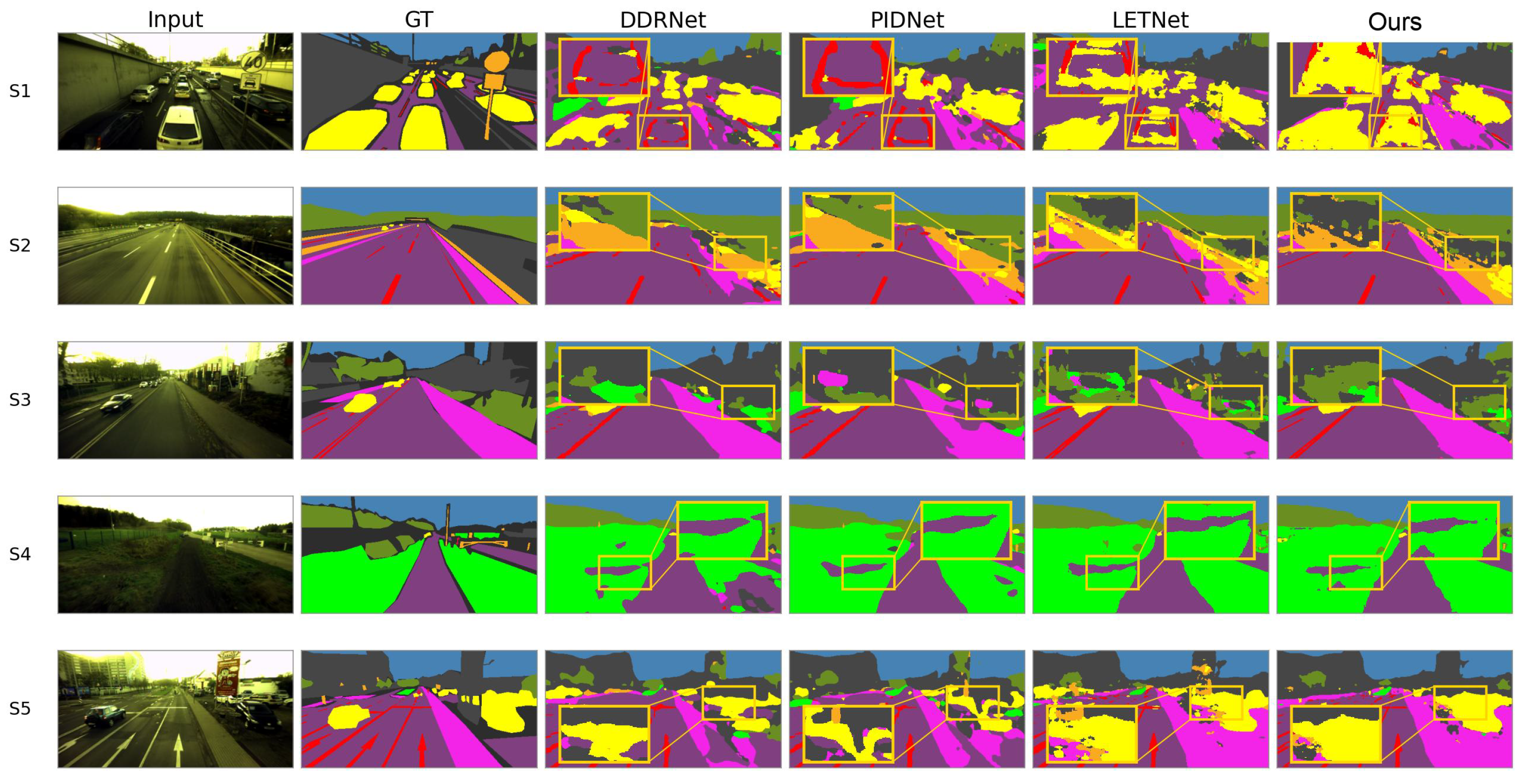
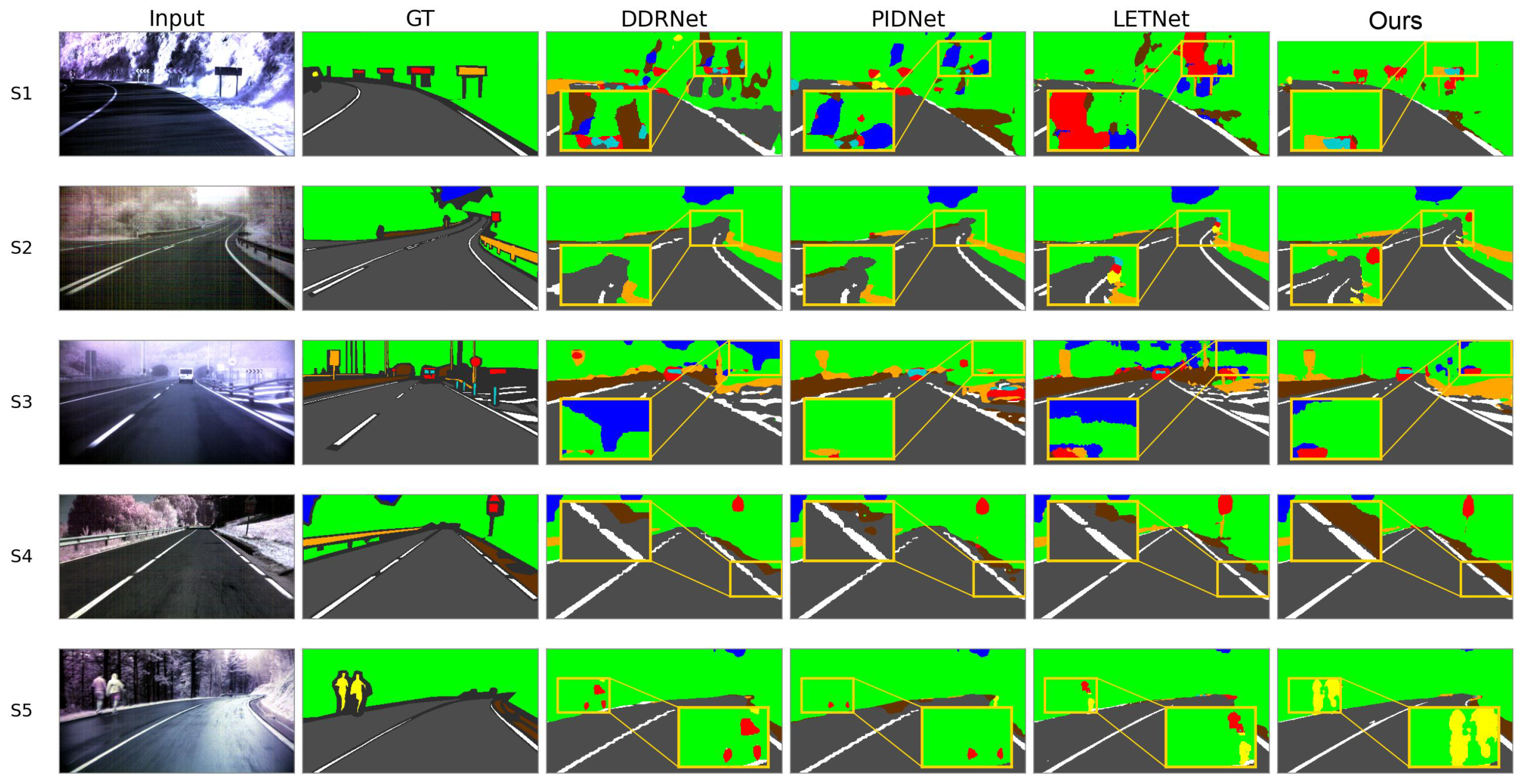
Figure 6 presents representative HyKo2 predictions. In these scenes, our method produces spatially coherent regions while preserving road boundaries, thin lane markings, and small foreground objects more consistently than the efficient baselines.

Figure 6. Qualitative comparison on HyKo2. S1–S5 denote five test scenes. Rows show the false-color input, ground truth, and predictions from DDRNet-23-slim, PIDNet-S, LETNet, and Ours. Yellow boxes and in-panel insets enlarge the same local region. Semantic colors follow the HyKo2 palette defined in Figure 5; ignored pixels are displayed in dark gray.

Figure 7 shows the corresponding comparison on HSI-Drive. The proposed network reduces fragmented predictions around vehicles and road markings and maintains compact responses over large road regions, indicating that the quantitative gains extend across both test sets.

Figure 7. Qualitative comparison on HSI-Drive. S1–S5 denote five test scenes. Rows show the false-color input, ground truth, and predictions from DDRNet-23-slim, PIDNet-S, LETNet, and Ours. Yellow boxes and in-panel insets enlarge the same local region. Semantic colors follow the HSI-Drive palette defined in Figure 5; ignored pixels are displayed in dark gray.

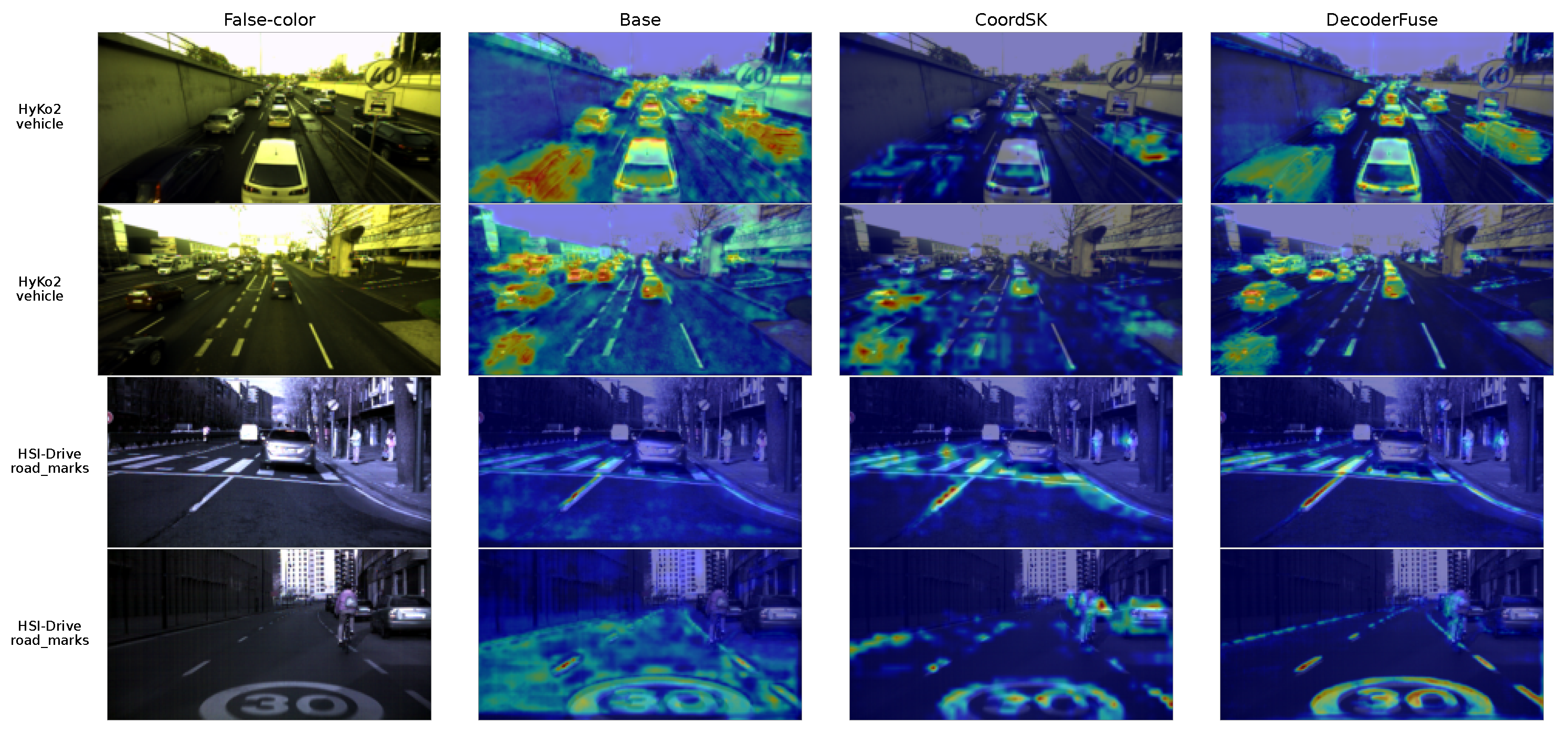
Figure 8 visualizes class-specific attribution using gradient-weighted class activation mapping (Grad-CAM) [35]. The models are compared on the same samples and target classes. In the illustrated examples, the complete network shows more concentrated responses on vehicles in HyKo2 and road markings in HSI-Drive. Section 4.6 complements these examples with quantitative localization metrics and representative missed-target cases.

Figure 8. Class-specific Grad-CAM attribution maps for the Base model and the complete network on matched test samples. The target classes are vehicles in HyKo2 and road markings in HSI-Drive. Complete-network maps are shown at the last CoordSK block and the DecoderFuse stage. Warmer colors indicate stronger relative attribution within each map.

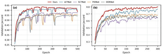
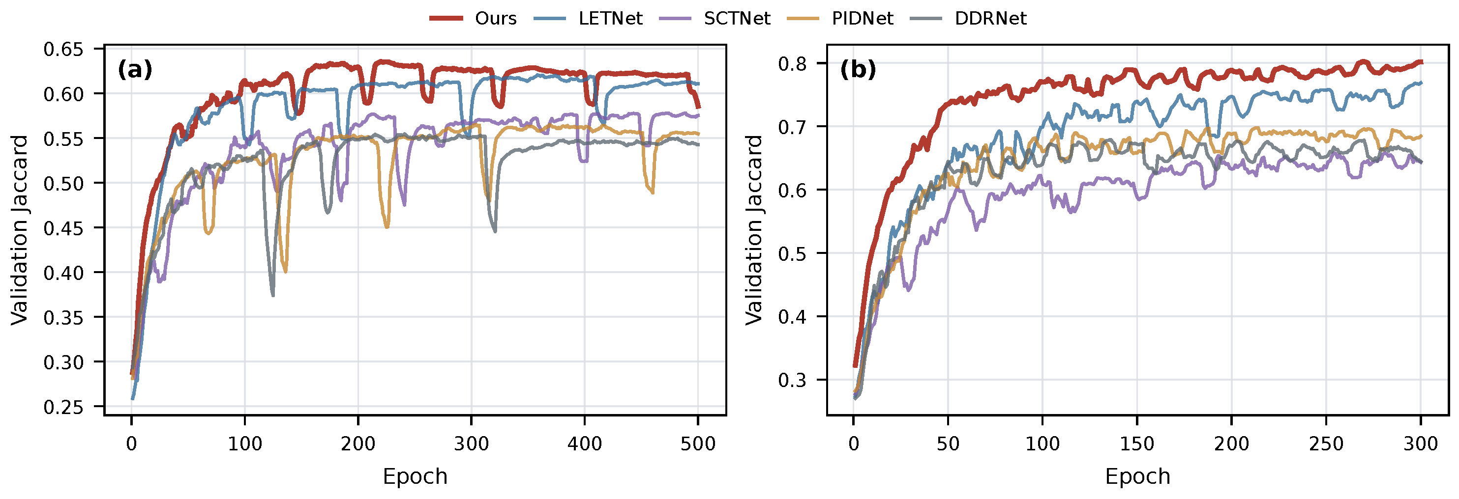
Figure 9 reports the optimization behavior under the common evaluation protocol. The curves show that our method reaches competitive validation Jaccard values on both datasets and remains stable toward the end of training.

Figure 9. Validation Jaccard convergence. (a) HyKo2. (b) HSI-Drive. The curves show the training behavior of our method and representative efficient baselines under the same evaluation protocol.

4.4. Ablation Studies

Table 7 examines the contribution of the proposed modules. D denotes DecoderFuse, S denotes the Spectral Token Stem, and C denotes CoordSK. All variants follow the same full-epoch training and evaluation protocol.

Table 7. Component ablation. (a) Segmentation accuracy. (b) Base computational complexity. D, S, and C denote DecoderFuse, the Spectral Token Stem, and CoordSK, respectively. J, $F_1$, Acc_M, and Acc_μ denote Jaccard index, macro F1, macro accuracy, and micro accuracy. Bold numerical values indicate the highest segmentation score for each metric within each dataset.

(a) Segmentation accuracy
Config.	HyKo2				HSI-Drive
	J	${\mathit{F}}_{\mathbf{1}}$	AccM	Accμ	J	${\mathit{F}}_{\mathbf{1}}$	AccM	Accμ
Base	0.6113	0.7181	0.7051	0.8774	0.7029	0.8094	0.7818	0.9555
Base + D + C	0.6436	0.7429	0.7344	0.8974	0.8123	0.8895	0.8648	0.9667
Base + D + S	0.6470	0.7451	0.7341	0.8993	0.7749	0.8650	0.8426	0.9680
Base + D + S + C	0.6670	0.7694	0.7551	0.9043	0.8181	0.8948	0.8755	0.9768
(b) Base computational complexity
Dataset	Input($\mathit{C}\mathbf{\times }\mathit{H}\mathbf{\times }\mathit{W}$)		Parameters		GMACs		GFLOPs
HyKo2	$15\times 254\times 510$		337,835		5.467		10.934
HSI-Drive	$25\times 216\times 409$		340,682		4.152		8.304

Parameters include all trainable weights and residual scales. THOP estimates the registered-operator MAC count for batch-one native inputs, with internal padding to $256\times 512$ for HyKo2 and $224\times 416$ for HSI-Drive. The Base FLOP estimates use two operations per MAC, so GFLOPs $=2$ × GMACs.

Base uses a four-stage encoder with channel widths of 32, 64, 96 and 128, and three decoder fusion stages. Its stem consists of a $3\times 3$ convolution, a $3\times 3$ depthwise convolution, and a $1\times 1$ projection. Six local residual blocks use pointwise–depthwise–pointwise convolutions. Each ungated decoder stage aligns channels, bilinearly upsamples the deep feature, and concatenates the features before a $1\times 1$ projection. Table 7b reports its parameter count and computational complexity.

The complete Base + D + S + C model gives the strongest scores across all four metrics on both datasets. Adding CoordSK to Base + D + S improves Jaccard by 1.99 points on HyKo2 and 4.32 points on HSI-Drive, while adding the Spectral Token Stem to Base + D + C improves Jaccard by 2.34 and 0.59 points. These results identify early spectral tokenization and coordinate-selective high-resolution mixing as the two effective architectural contributions, with DecoderFuse serving as the lightweight reconstruction module.

Table 8 examines the descriptor groups inside the Spectral Token Stem. The Pool + Norm + Stats row corresponds to the default setting used in Table 1 and Table 7. Moving from Stats only to Norm + Stats slightly improves HyKo2 Jaccard from 0.6599 to 0.6606 and improves HSI-Drive Jaccard from 0.7859 to 0.8007. Adding pooled spectral tokens further raises the scores to 0.6670 and 0.8181, respectively. These results show that progressively incorporating normalized descriptors and pooled spectral tokens improves the overall performance of the stem.

Table 8. Descriptor ablation of the Spectral Token Stem. Pool, Norm, and Stats denote pooled spectral tokens, normalized spectral descriptors, and band-wise statistical descriptors, respectively. The Pool + Norm + Stats row is the default stem used in the main comparison. A check mark indicates that the corresponding descriptor group is included. Bold numerical values indicate the highest score for each metric within each dataset.

Variant	Pool	Norm	Stats	HyKo2				HSI-Drive
				$\mathit{J}$	${\mathit{F}}_{\mathbf{1}}$	AccM	Accμ	$\mathit{J}$	${\mathit{F}}_{\mathbf{1}}$	AccM	Accμ
Stats only			✔	0.6599	0.7657	0.7519	0.8996	0.7859	0.8723	0.8512	0.9717
Norm + Stats		✔	✔	0.6606	0.7692	0.7522	0.9023	0.8007	0.8816	0.8694	0.9748
Pool + Norm + Stats	✔	✔	✔	0.6670	0.7694	0.7551	0.9043	0.8181	0.8948	0.8755	0.9768

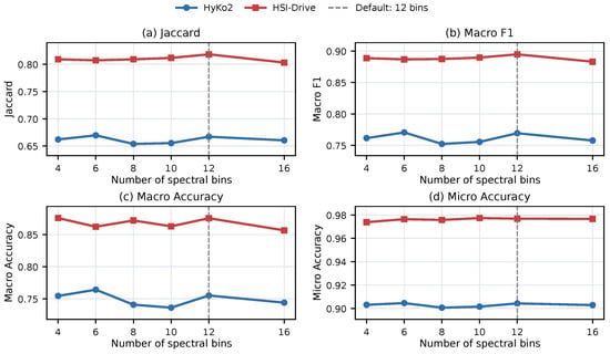
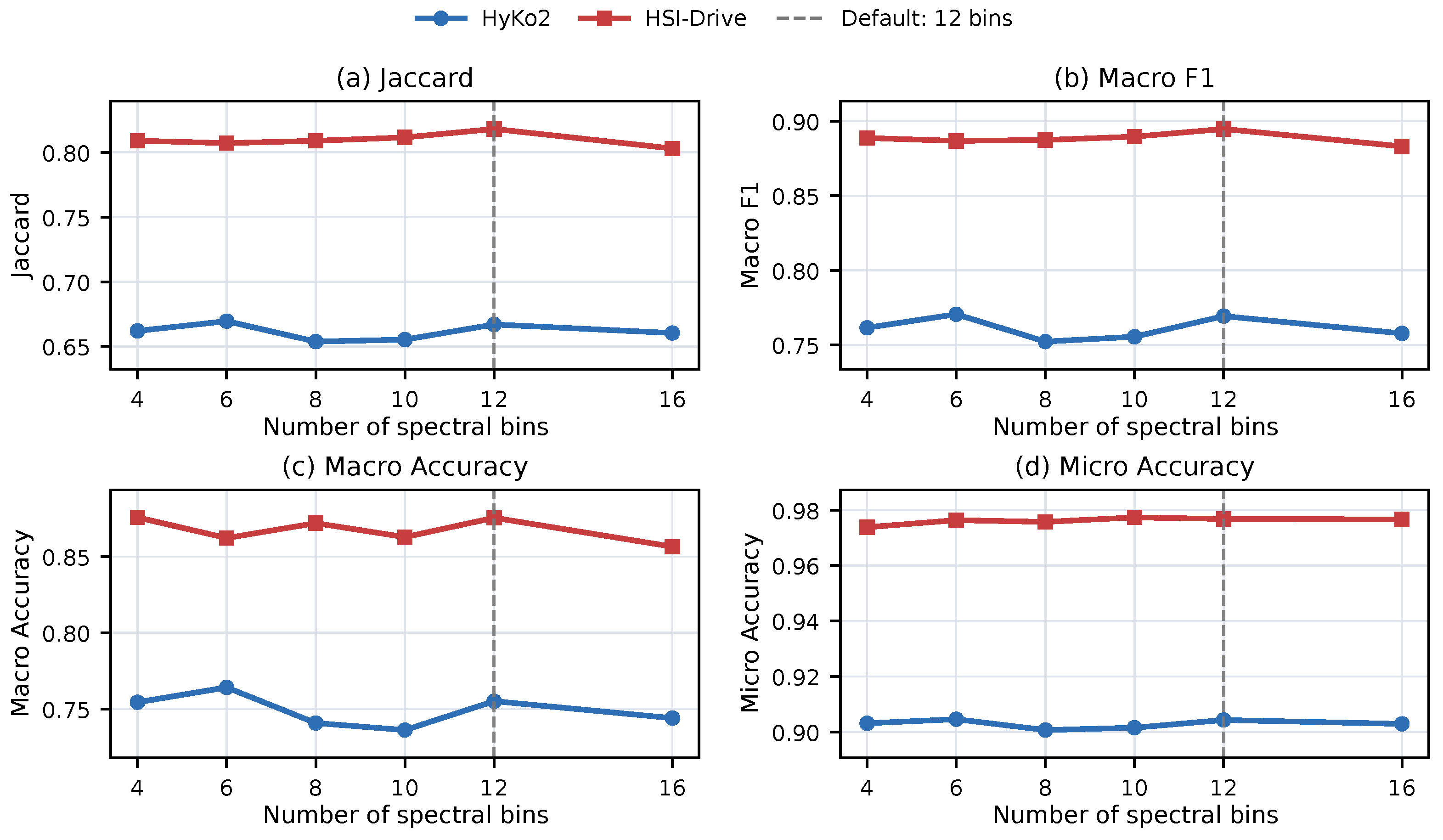
Using the Pool + Norm + Stats descriptor set, Figure 10 studies the number of pooled spectral bins. The effect of bin count varies across the two datasets. Using six bins gives slightly higher Jaccard on HyKo2 than 12 bins, whereas using 12 bins achieves the highest Jaccard on HSI-Drive while retaining competitive HyKo2 performance. Increasing the bin count to 16 does not improve Jaccard on either dataset relative to 12 bins. With 12 bins in each of the Pool and Norm branches and four Stats channels, the concatenated descriptor contains 28 channels, compared with 36 channels at 16 bins. We therefore adopt 12 bins as the common default, balancing segmentation performance across the two datasets and descriptor dimensionality.

Figure 10. Bin-count trends for the Pool + Norm + Stats Spectral Token Stem. (a) Jaccard. (b) Macro F1. (c) Macro accuracy. (d) Micro accuracy. The vertical dashed line marks the default setting of 12 bins.

Table 4 compares the Full hyperspectral cube with low-dimensional input representations. Raw hyperspectral input gives the strongest result on both datasets, reaching 0.6670 Jaccard on HyKo2 and 0.8181 on HSI-Drive. PCA3 preserves part of the spectral information, but it reduces Jaccard by 4.45 points on HyKo2 and 3.73 points on HSI-Drive. Pseudo-RGB is closer on HyKo2, where the Jaccard gap is 1.82 points, but it drops sharply on HSI-Drive with an 18.55-point Jaccard gap. These results support in-network spectral compression instead of replacing the hyperspectral cube before learning.

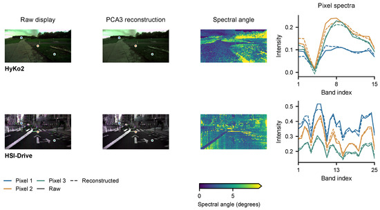
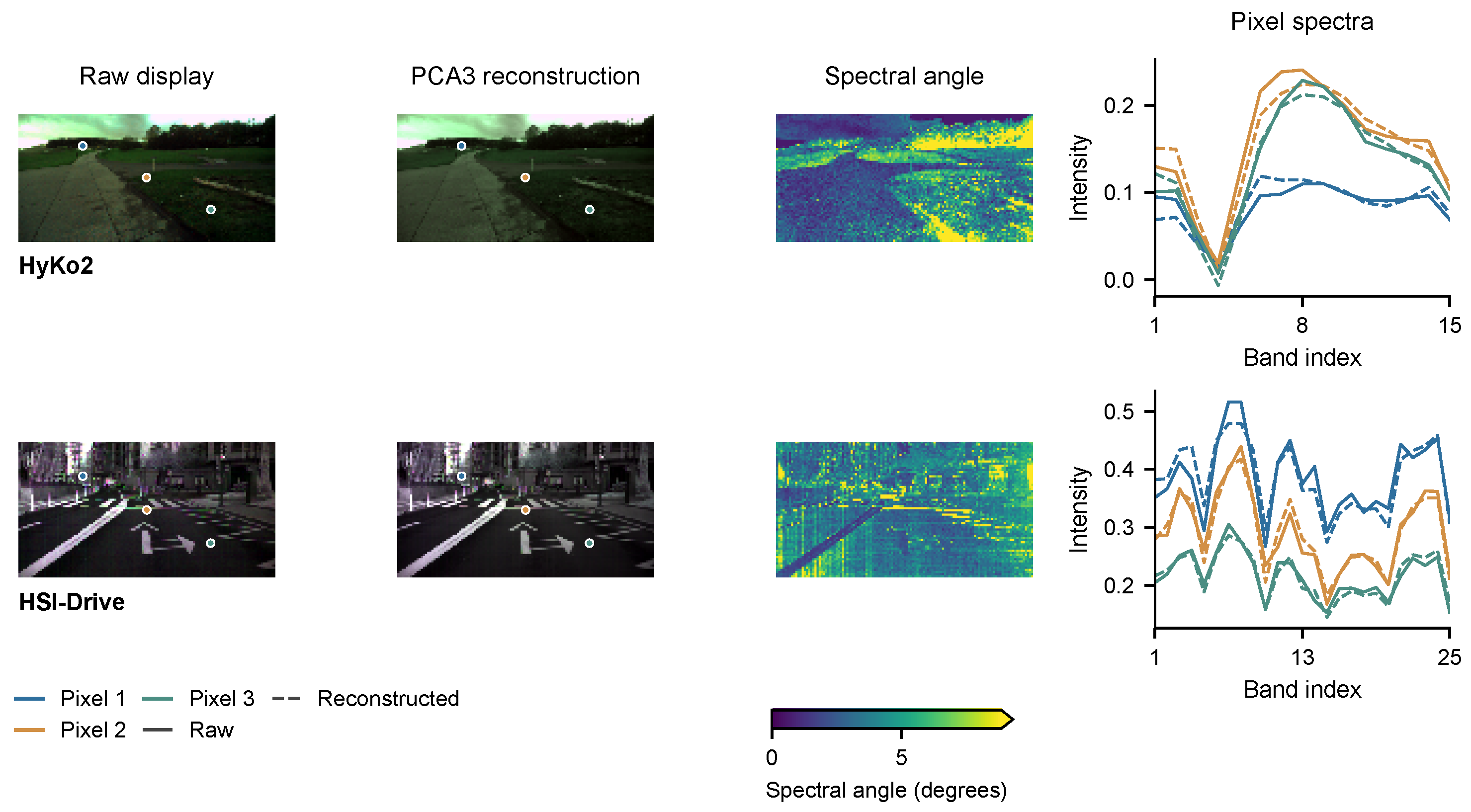
The input-representation study shows higher segmentation performance with Full hyperspectral input than with either reduced representation. Additional PCA3 variance and reconstruction analyses are reported in Table 9 and Figure 11. The proposed network instead converts the raw spectral evidence into compact tokens before the wider spatial stages, allowing the subsequent CoordSK blocks and shallow decoder to operate on compact spectral–spatial representations.

Table 9. Dataset-level PCA3 variance retention and inverse-reconstruction statistics, pooled across the training, validation, and test splits.

Dataset	Retained Variance (%)			RSE	SAM
	Mean	Median	5th–95th Percentile	($\times {\mathbf{10}}^{-\mathbf{3}}$)	(°)
HyKo2	99.79	99.80	99.64–99.93	0.7937	2.81
HSI-Drive	98.52	99.06	96.01–99.71	1.2769	4.29

All three splits are pooled within each dataset. Retention summaries weight images equally; medians and percentiles are computed from the pooled image values. RSE divides summed squared residuals by summed raw-spectrum energy over non-ignored pixels. SAM is the pixel-weighted mean over non-ignored spectrum pairs with nonzero norms.

Figure 11. Paired raw and PCA3-reconstructed observations for the first test image in sorted order from each dataset. Display bands are R15/G8/B1 for HyKo2 and R25/G13/B1 for HSI-Drive. Within each pair, the raw-derived 1st–99th percentile channel stretch is shared, without cropping. Spectral-angle maps share a scale capped at the 95th percentile of finite angles from these two images; higher values are indicated by the color bar extension. Solid and dashed curves show raw and reconstructed spectra at the three marked, predefined pixels. Blue, orange, and green markers identify Pixels 1, 2, and 3, respectively; the corresponding spectra use the same colors.

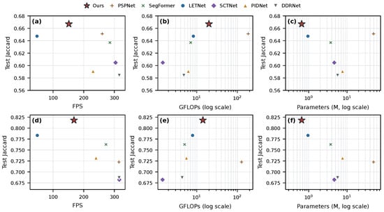
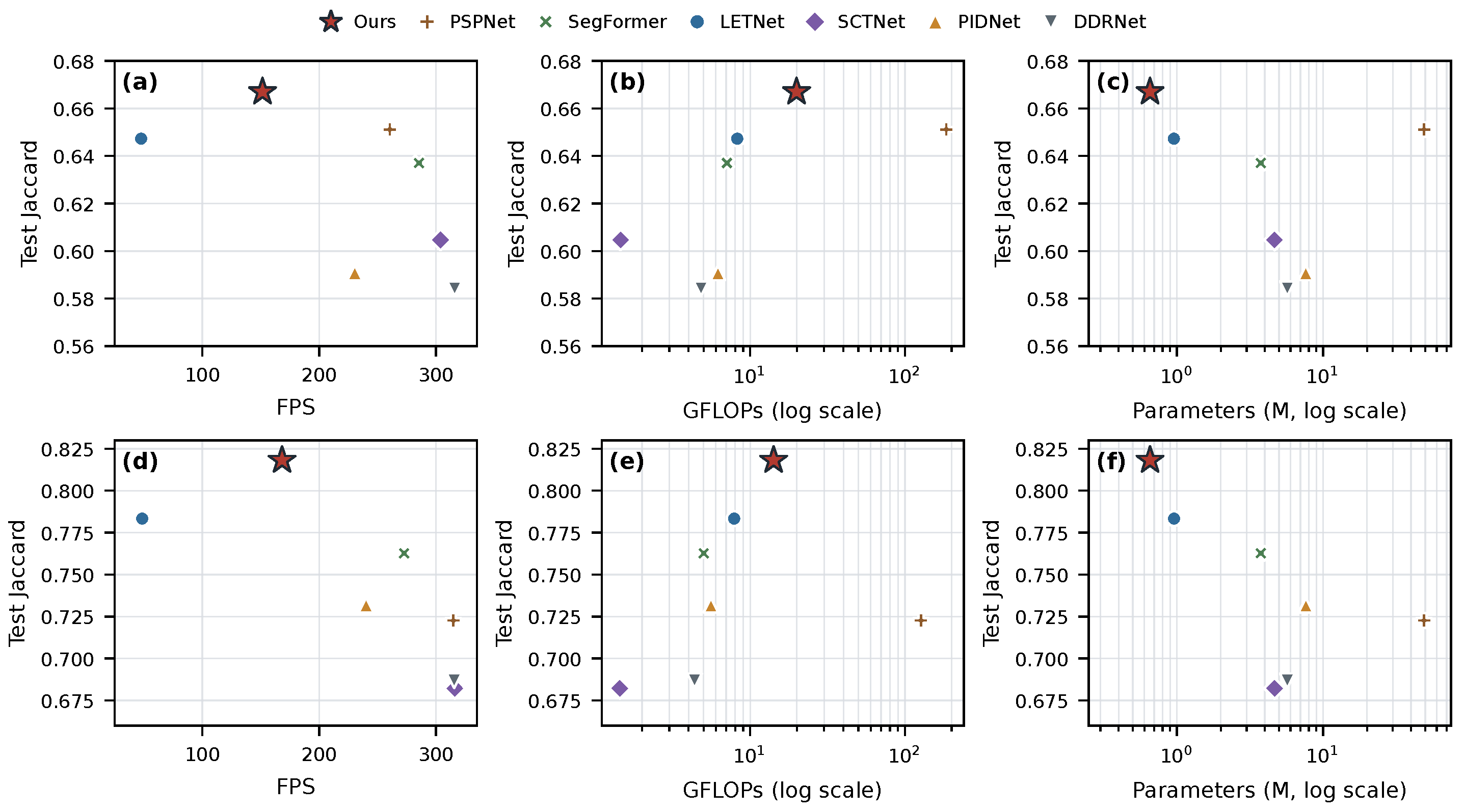
Figure 12 and Table 2 summarize throughput, complexity, and parameter count. Our method uses 0.656 million parameters and achieves higher Jaccard than the baselines in Table 1 on both datasets. DDRNet-23-slim and SCTNet-S run faster on the RTX 5090, but they sacrifice accuracy; compared with LETNet, our method is 3.18 times faster on HyKo2 and 3.47 times faster on HSI-Drive while also achieving higher Jaccard.

Figure 12. Accuracy–efficiency trade-offs. (a,d) Test Jaccard versus FP32 throughput for single-image inference. (b,e) Test Jaccard versus GFLOPs. (c,f) Test Jaccard versus trainable parameters. The top row corresponds to HyKo2 and the bottom row corresponds to HSI-Drive; logarithmic horizontal axes are used for GFLOPs and parameters.

The GFLOPs comparison represents arithmetic cost, whereas FPS reflects the realized throughput of each implementation on the tested GPU. The two indicators are therefore interpreted together. This operating point is relevant to spectral imaging systems with limited computational budgets, including intelligent vehicles, mobile spectral cameras, and embedded inspection devices, where model size, operator design, arithmetic complexity, and single-image throughput jointly determine practical performance.

Table 3 quantifies the computation allocated to each selected module group. The six CoordSK blocks occupy 45.90% and 45.77% of the instrumented forward time on HyKo2 and HSI-Drive, respectively; the three DecoderFuse blocks occupy 12.98% and 18.24%. The Full reference has complete-inference latencies of 6.855 and 5.976 ms, compared with 20.896 and 21.191 ms for LETNet, giving throughput ratios of 3.05 and 3.55. Its THOP estimates are 9.298/6.608 GMACs, versus 4.124/3.937 for LETNet. These registered-operator MAC estimates and measured GPU latencies provide complementary measures of computational efficiency. The profiling identifies CoordSK as the largest of the three measured module groups.

Table 6 compares DecoderFuse with Add and Concat on HyKo2 and HSI-Drive. Add combines the aligned shallow and deep features by element-wise addition. Concat applies concatenation followed by a $1\times 1$ projection and CBAM attention. The DecoderFuse row uses the complete-network reference with the mean-absolute-intensity Stats configuration.

DecoderFuse achieved the highest Jaccard and macro accuracy among the three strategies on both datasets. On HyKo2, it led all four metrics, with Jaccard gains of 0.93 and 0.84 percentage points over Add and Concat, respectively. The corresponding macro F1 gains were 1.18 and 1.17 percentage points.

On HSI-Drive, DecoderFuse achieved 0.8030 Jaccard and 0.8696 macro accuracy. Its macro accuracy exceeded Add and Concat by 0.17 and 1.05 percentage points, respectively. Add achieved the highest macro F1 and micro accuracy on this dataset. Across both datasets, the most consistent advantages of DecoderFuse were in region overlap and class-averaged accuracy.

To quantify descriptor overlap and spectral-information preservation, we evaluated the deterministic descriptors at 12 bins before learned smoothing and spatial projection. Stats comprised the mean, population standard deviation, range, and mean absolute difference between adjacent bands. Each training and test image contributed 512 uniformly sampled pixels without replacement using seed 42. Linear centered kernel alignment (CKA) [36] was computed on column-centered training descriptors. For reconstruction, a ridge map with a fixed penalty of ${10}^{-6}$ was fitted to training descriptors standardized using training-set statistics and applied to the sampled test spectra. Relative squared error (RSE) was the summed squared reconstruction residual divided by the summed squared raw spectra. The spectral angle mapper (SAM) metric was averaged in degrees over spectrum pairs with nonzero norms.

Table 10 shows substantial overlap between Pool and Stats, with CKA above 0.98 on both datasets. The similarity involving Norm was dataset dependent. On HyKo2, Norm retained relatively high similarity to the other groups, whereas its CKA with Pool and Stats was below 0.015 on HSI-Drive. This pattern identifies shared variation between Pool and Stats and a more distinct normalized representation on HSI-Drive.

Table 10. Linear CKA between descriptor groups at 12 bins, computed on sampled training pixels before learned smoothing and projection. Higher values indicate greater representational similarity.

Descriptor Pair	HyKo2	HSI-Drive
Pool/Norm	0.7848	0.0102
Pool/Stats	0.9936	0.9849
Norm/Stats	0.7860	0.0147

Table 11 shows that Pool + Norm + Stats achieved the lowest RSE and SAM among the evaluated combinations on both datasets. Adding Stats to Pool + Norm reduced RSE by approximately 4% on HyKo2 and 12% on HSI-Drive. Thus, the high Pool–Stats similarity coexisted with additional recoverable spectral information. These reconstruction results support combining partly overlapping descriptors to preserve spectral information in the Spectral Token Stem.

Table 11. Raw-spectrum reconstruction from six descriptor combinations at 12 bins. The ridge map is fitted on sampled training pixels and evaluated on sampled test pixels. Lower RSE and SAM indicate better reconstruction; bold values are the lowest among the evaluated combinations.

Descriptor Combination	HyKo2		HSI-Drive
	RSE	SAM (°)	RSE	SAM (°)
Pool	$1.4418\times {10}^{-6}$	0.1017	$6.5405\times {10}^{-4}$	3.5230
Norm	$4.3506\times {10}^{-2}$	9.1561	$5.4722\times {10}^{-1}$	7.4937
Stats	$3.6987\times {10}^{-3}$	5.5104	$2.5944\times {10}^{-3}$	6.0083
Pool + Norm	$1.0340\times {10}^{-6}$	0.0992	$6.3819\times {10}^{-4}$	4.1064
Norm + Stats	$1.6752\times {10}^{-3}$	4.1184	$1.9288\times {10}^{-3}$	9.2240
Pool + Norm + Stats	$\mathbf{9.9377}\times {\mathbf{10}}^{-\mathbf{7}}$	0.0975	$\mathbf{5.6192}\times {\mathbf{10}}^{-\mathbf{4}}$	3.4881

To examine the spectral information preserved by PCA3, we analyzed all 914 images using the HS3-Bench per-image fitting protocol [17]. Each image’s pixel spectra were centered, and PCA retained three components without band scaling or whitening. Retained variance was the fraction of total centered spectral variance explained by these components. Scores were inverse-transformed in their native precision, and reconstruction was evaluated using RSE and SAM as defined above. This diagnostic used scikit-learn 1.8.0 with the resolved covariance eigendecomposition solver.

Table 9 summarizes all three splits for each dataset. Mean image-level variance retention was 99.79% on HyKo2 and 98.52% on HSI-Drive. The corresponding mean reconstruction angles were 2.81 and 4.29 degrees. HSI-Drive image-level retention ranged from 74.65% to 99.92%, indicating variation across scenes despite the high average retention.

Figure 11 compares the paired displays, spatial angle maps, and pixel spectra. The displays preserved similar scene structure, while the angle maps and spectra exposed residual differences. Together with Table 4, these results show that high overall variance retention did not guarantee equivalent segmentation performance. Full hyperspectral input retained higher Jaccard on both datasets, supporting learned spectral compression within the network.

4.5. Comparison with a Pretrained Foundation Model

Table 5 compares HSI-Adapter [4] with the proposed network, reusing the four test metrics reported for ours in Table 1. Our network was trained from scratch, while HSI-Adapter retained a frozen DINOv2 ViT-B/14 pretrained backbone and its dataset-specific architecture. Both methods used raw hyperspectral inputs and training budgets of 500 epochs on HyKo2 and 300 epochs on HSI-Drive. HSI-Adapter used seed 42 and batch size 2, with checkpoints selected by validation Jaccard and test predictions evaluated on the native image grids.

The adapted HSI-Adapter recipe used AdamW with a learning rate of ${10}^{-4}$, weight decay of 0.05, and the official parameter groups. Gradient clipping used a maximum norm of 0.01; the loss combined main cross-entropy with auxiliary cross-entropy weighted by 0.4. HyKo2 used linear warm-up followed by cosine scheduling, whereas HSI-Drive used multistep decay. Fixed resizing was used without horizontal-flip augmentation. Its internal grids were $448\times 896$ for HyKo2 and $224\times 448$ for HSI-Drive, with output logits interpolated once to the native grid. The epoch budgets replaced the upstream 80,000-iteration budget. The comparison therefore covers complete model recipes with different pretraining, optimization, and internal input grids.

Our network uses 0.656 million trainable parameters, less than 0.5% of HSI-Adapter’s total parameter count. HSI-Adapter achieves Jaccard scores of 0.7331 and 0.9060 on HyKo2 and HSI-Drive with its larger pretrained model, compared with 0.6670 and 0.8181 for our network. Table 5 quantifies the accuracy–model-size trade-off. Together with the throughput measurements in Table 2, these results position the proposed network as a compact design for hyperspectral segmentation under computational constraints.

4.6. Class-Specific Localization and Failure Cases

We quantified Grad-CAM localization using a plain Base with a convolutional stem, local convolution blocks, and ungated fusion. Full denotes the complete configuration evaluated in Table 6. Both models were evaluated at the pre-classifier feature layer, using the whole-image sum of target-class logits as the attribution score. Ground-truth labels were used only for localization evaluation. Present, nonignored classes with at least 64 labeled pixels were included. The paired comparison covered all 49 HyKo2 and 151 HSI-Drive test images, yielding 340 and 945 nondegenerate image–class regions, respectively. One degenerate Base map on HSI-Drive was excluded from both sides of the paired comparison.

Table 12 summarizes the quantitative localization results. Each metric was averaged with equal weight per image–class region. Target mass is the fraction of valid-pixel attribution inside the target. Normalized mass divides target mass by the target’s valid-area fraction; a uniform response yields one. Peak hit records whether the strongest valid response lies inside the target. Top-10% precision is the target fraction among the highest 10% of valid responses.

Table 12. Quantitative Grad-CAM localization on paired test image–class regions. Higher values indicate better localization; bold entries mark the higher mean within each dataset.

Dataset	Model	Target Mass (%)	Normalized Mass	Peak Hit (%)	Top-10% Precision (%)
HyKo2	Base	72.10	19.49	91.47	64.47
HyKo2	Full	75.89	25.73	89.12	65.09
HSI-Drive	Base	67.57	27.67	80.11	47.16
HSI-Drive	Full	71.17	32.38	84.76	48.29

The Full configuration increased average target mass by 3.79 percentage points on HyKo2 and 3.60 percentage points on HSI-Drive. Normalized mass also increased on both datasets, indicating greater attribution concentration after accounting for target area. The Full configuration achieved higher top-10% precision on both datasets and higher peak-hit rate on HSI-Drive. HyKo2 peak-hit rates were 91.47% for Base and 89.12% for Full. Region-level concentration and peak-hit measurements capture complementary aspects of localization. The Full configuration concentrates more attribution within target regions on both datasets.

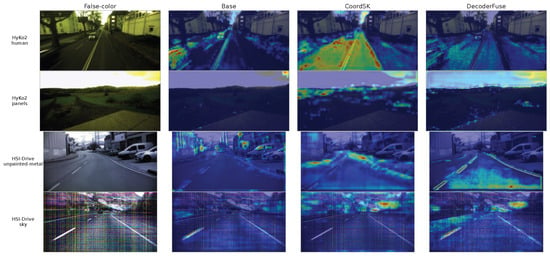
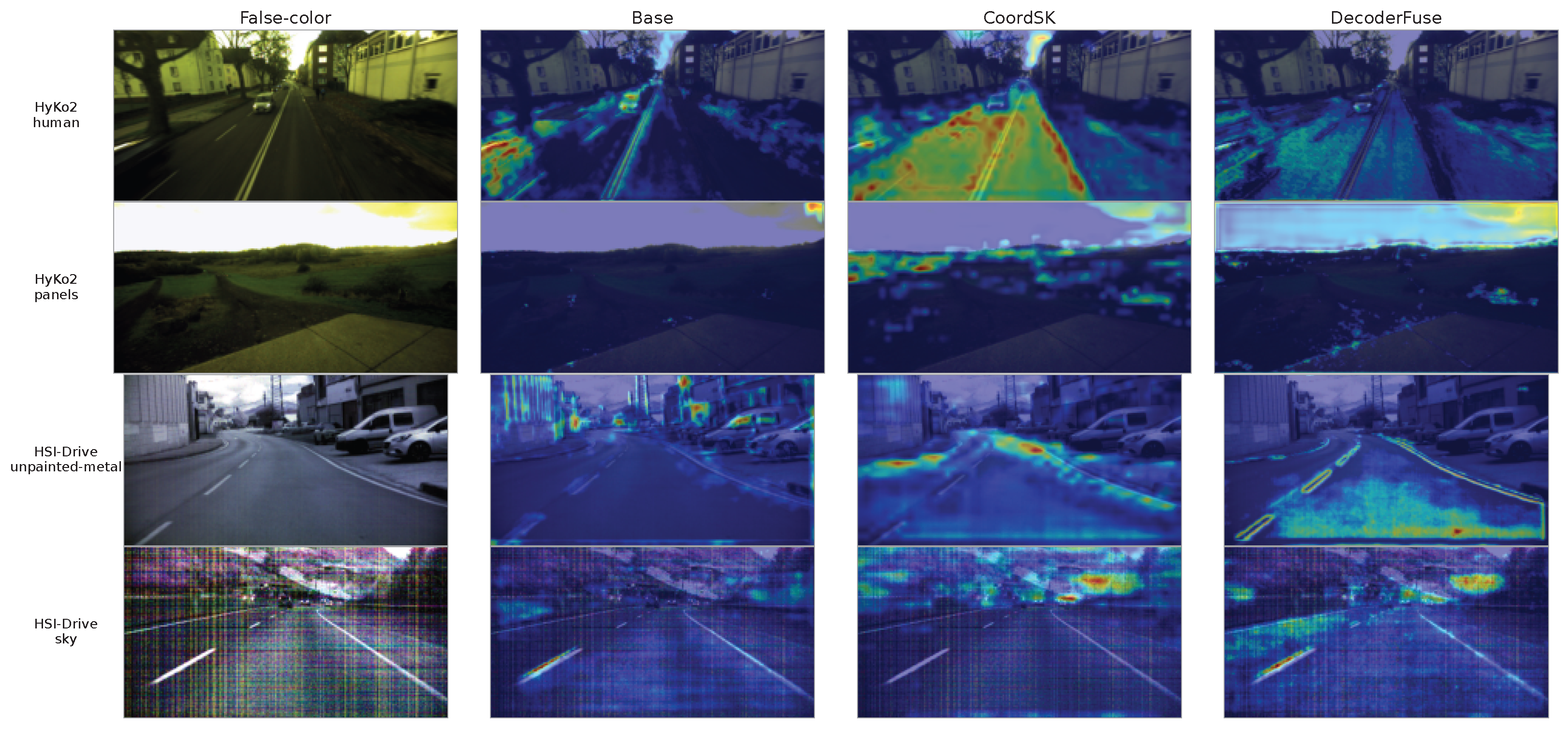
Figure 13 shows four missed-target cases using the display protocol of Figure 8. The attribution score sums target-class logits inside the labeled region, with the same target region used for both models. Base maps use the decoder projection; Full maps use the last CoordSK block and DecoderFuse projection. Full correctly segmented none of the selected target pixels, and every valid-region DecoderFuse peak fell outside the labeled target.

Figure 13. Representative missed-target cases: human and panels in HyKo2, and unpainted metal and sky in HSI-Drive, from top to bottom. Columns show the false-color input, Base decoder attribution, Full CoordSK attribution, and Full DecoderFuse attribution. Warmer colors indicate stronger relative attribution within each map.

The failures reveal small-area target misses and class confusion. The HyKo2 human region occupied only 191 pixels (0.15% of the image), with 85.9% misclassified as panels. In the second HyKo2 case, 96.8% of panel pixels were classified as building. On HSI-Drive, 92.3% of unpainted-metal pixels were classified as painted metal, while the 124-pixel sky region was classified as vegetation. These local failures identify small-target recognition and material-category discrimination as priorities for further improvement.

4.7. Limitations and Future Work

The evaluation covers two public ground-based hyperspectral benchmarks, with inference measured on an RTX 5090. Further validation across sensors, acquisition ranges, weather and illumination conditions, and automotive embedded accelerators will test transfer to broader deployment settings. Temporal cues from sequential hyperspectral acquisition offer a further route to scene consistency while preserving efficient inference.

5. Conclusions

This paper presented an efficient semantic segmentation network for ground-based hyperspectral imagery that combines early spectral tokenization, coordinate-selective high-resolution mixing, and lightweight guided decoding. On HyKo2 and HSI-Drive, the proposed network achieves Jaccard indices of 0.6670 and 0.8181 with 0.656 million parameters. The component, bin-count, and input-representation studies show that preserving raw spectral evidence and learning compact spectral–spatial features inside the network are important for the final accuracy–efficiency balance. The results indicate that a compact spectral–spatial network can improve segmentation accuracy over representative efficient baselines while maintaining high single-image throughput on an RTX 5090. These results support a compact spectral–spatial design that preserves raw hyperspectral evidence and combines directional context with adaptive local-scale processing for efficient ground-based scene understanding.

References

- Yu, C.; Gao, C.; Wang, J.; Yu, G.; Shen, C.; Sang, N. BiSeNet V2: Bilateral Network with Guided Aggregation for Real-Time Semantic Segmentation. Int. J. Comput. Vis. 2021, 129, 3051–3068. [Google Scholar] [CrossRef] [Scilit]
- Pan, H.; Hong, Y.; Sun, W.; Jia, Y. Deep Dual-Resolution Networks for Real-Time and Accurate Semantic Segmentation of Traffic Scenes. IEEE Trans. Intell. Transp. Syst. 2023, 24, 3448–3460. [Google Scholar] [CrossRef] [Scilit]
- Xu, A.; Xue, Z.; Li, Z.; Cheng, S.; Su, H.; Xia, J. UM2Former: U-Shaped Multimixed Transformer Network for Large-Scale Hyperspectral Image Semantic Segmentation. IEEE Trans. Geosci. Remote Sens. 2025, 63, 1–21. [Google Scholar] [CrossRef] [Scilit]
- Hurtado, J.V.; Mohan, R.; Valada, A. Hyperspectral Adapter for Semantic Segmentation with Vision Foundation Models. IEEE Robot. Autom. Lett. 2026, 11, 3606–3613. [Google Scholar] [CrossRef] [Scilit]
- Shah, I.A.; Li, J.; Brophy, T.; Glavin, M.; Jones, E.; Ward, E.; Deegan, B. Multi-Scale Spectral Attention Module-Based Hyperspectral Segmentation in Autonomous Driving Scenarios. arXiv 2025, arXiv:2506.18682. [Google Scholar] [CrossRef] [Scilit]
- Fan, M.; Lai, S.; Huang, J.; Wei, X.; Chai, Z.; Luo, J.; Wei, X. Rethinking BiSeNet for Real-Time Semantic Segmentation. In Proceedings of the IEEE/CVF Conference on Computer Vision and Pattern Recognition, Virtual Event, 19–25 June 2021; pp. 9716–9725. [Google Scholar]
- Xu, J.; Xiong, Z.; Bhattacharyya, S.P. PIDNet: A Real-time Semantic Segmentation Network Inspired by PID Controllers. In Proceedings of the IEEE/CVF Conference on Computer Vision and Pattern Recognition, Vancouver, BC, Canada, 17–24 June 2023; pp. 19529–19539. [Google Scholar] [CrossRef] [Scilit]
- Meng, P.; Jia, S.; Li, Q. DMBR-Net: Deep Multiple-Resolution Bilateral Network for Real-Time and Accurate Semantic Segmentation. Complex Intell. Syst. 2023, 9, 6427–6436. [Google Scholar] [CrossRef] [Scilit]
- Xu, G.; Li, J.; Gao, G.; Lu, H.; Yang, J.; Yue, D. Lightweight Real-Time Semantic Segmentation Network with Efficient Transformer and CNN. IEEE Trans. Intell. Transp. Syst. 2023, 24, 15897–15906. [Google Scholar] [CrossRef] [Scilit]
- Xu, Z.; Wu, D.; Yu, C.; Chu, X.; Sang, N.; Gao, C. SCTNet: Single-Branch CNN with Transformer Semantic Information for Real-Time Segmentation. Proc. Aaai Conf. Artif. Intell. 2024, 38, 6378–6386. [Google Scholar] [CrossRef] [Scilit]
- Gu, Y.; Fu, C.; Song, W.; Wang, X.; Chen, J. RTLinearFormer: Semantic Segmentation with Lightweight Linear Attentions. Neurocomputing 2025, 625, 129489. [Google Scholar] [CrossRef] [Scilit]
- Lei, X.; Pan, Y.; Zhang, Y.; Jiang, Z. DSARFormer: A Dynamic Sparse Axial Rectangular Transformer for Real-Time Semantic Segmentation. Signal Image Video Process. 2025, 19, 778. [Google Scholar] [CrossRef] [Scilit]
- Wang, Y.; Qing, Y.; Fang, Z.; Zhao, X. LCS4: Linear Complexity State-Space Transformers With Multiscale Overlapping Scans for Efficient Semantic Segmentation. IEEE Trans. Instrum. Meas. 2025, 74, 1–13. [Google Scholar] [CrossRef] [Scilit]
- Gutierrez-Zaballa, J.; Basterretxea, K.; Echanobe, J.; Martinez, M.V.; del Campo, I. Exploring Fully Convolutional Networks for the Segmentation of Hyperspectral Imaging Applied to Advanced Driver Assistance Systems. In Proceedings of the 15th International Workshop on Design and Architecture for Signal and Image Processing (DASIP 2022), Budapest, Hungary, 20–22 June 2022; pp. 136–148. [Google Scholar] [CrossRef] [Scilit]
- Gutierrez-Zaballa, J.; Basterretxea, K.; Echanobe, J.; Martinez, M.V.; Martinez-Corral, U.; Mata-Carballeira, O.; del Campo, I. On-Chip Hyperspectral Image Segmentation with Fully Convolutional Networks for Scene Understanding in Autonomous Driving. J. Syst. Archit. 2023, 139, 102878. [Google Scholar] [CrossRef] [Scilit]
- Shah, I.A.; Li, J.; Glavin, M.; Jones, E.; Ward, E.; Deegan, B. Hyperspectral Imaging-Based Perception in Autonomous Driving Scenarios: Benchmarking Baseline Semantic Segmentation Models. In Proceedings of the Workshop on Hyperspectral Imaging and Signal Processing: Evolution in Remote Sensing, Helsinki, Finland, 9–11 December 2024; pp. 1–5. [Google Scholar] [CrossRef] [Scilit]
- Theisen, N.; Bartsch, R.; Paulus, D.; Neubert, P. HS3-Bench: A Benchmark and Strong Baseline for Hyperspectral Semantic Segmentation in Driving Scenarios. In Proceedings of the IEEE/RSJ International Conference on Intelligent Robots and Systems, Abu Dhabi, United Arab Emirates, 14–18 October 2024; pp. 5895–5901. [Google Scholar] [CrossRef] [Scilit]
- Hong, D.; Han, Z.; Yao, J.; Gao, L.; Zhang, B.; Plaza, A.; Chanussot, J. SpectralFormer: Rethinking Hyperspectral Image Classification With Transformers. IEEE Trans. Geosci. Remote Sens. 2022, 60, 1–15. [Google Scholar] [CrossRef] [Scilit]
- Wang, C.; Miyazaki, D. MobileSACNet: Lightweight Spectral-Spatial Compression for Hyperspectral Segmentation in Autonomous Driving Systems. In Proceedings of the 19th International Conference on Machine Vision Applications, Kyoto, Japan, 26–28 July 2025. [Google Scholar] [CrossRef] [Scilit]
- Shah, I.A.; Li, J.; Delaney, E.; Ward, E.; Glavin, M.; Jones, E.; Deegan, B. Learnable Quantum Efficiency Filters for Urban Hyperspectral Segmentation. arXiv 2026, arXiv:2603.26528. [Google Scholar] [CrossRef] [Scilit]
- Yang, Z.; Yao, H.; Tian, L.; Zhao, X.; Li, Q.; Wang, Q. Intra- and Cross-Scale Feature Interaction Network for Referring Remote Sensing Image Segmentation. IEEE Trans. Geosci. Remote Sens. 2026, 64, 5629310. [Google Scholar] [CrossRef] [Scilit]
- Yang, Z.; Yao, H.; Wu, J.; Tian, L.; Ni, W.; Li, Q.; Wang, Q. Spatial-Semantic Alignment and Change-Aware Network for Remote Sensing Image Change Captioning. IEEE Trans. Geosci. Remote Sens. 2026, 64, 5621611. [Google Scholar] [CrossRef] [Scilit]
- Yang, Z.; Zhou, D.; Yang, Y.; Zhang, J.; Chen, Z. TransRoadNet: A Novel Road Extraction Method for Remote Sensing Images via Combining High-Level Semantic Feature and Context. IEEE Geosci. Remote Sens. Lett. 2022, 19, 1–5. [Google Scholar] [CrossRef] [Scilit]
- Yang, Z.; Yao, H.; Li, Q.; Ni, W.; Wu, J.; Wang, Q. Semantic–Spatial Feature Refinement Network for Road Extraction From Remote Sensing Images. IEEE Trans. Geosci. Remote Sens. 2026, 64, 1–10. [Google Scholar] [CrossRef] [Scilit]
- Basterretxea, K.; Martinez, V.; Echanobe, J.; Gutierrez-Zaballa, J.; del Campo, I. HSI-Drive: A Dataset for the Research of Hyperspectral Image Processing Applied to Autonomous Driving Systems. In Proceedings of the IEEE Intelligent Vehicles Symposium, Virtual, 11–17 July 2021; pp. 866–873. [Google Scholar] [CrossRef] [Scilit]
- Gutierrez-Zaballa, J.; Basterretxea, K.; Echanobe, J.; Martinez, M.V.; Martinez-Corral, U. HSI-Drive v2.0: More Data for New Challenges in Scene Understanding for Autonomous Driving. In Proceedings of the IEEE Symposium Series on Computational Intelligence, Mexico City, Mexico, 5–8 December 2023; pp. 207–214. [Google Scholar] [CrossRef] [Scilit]
- Ronneberger, O.; Fischer, P.; Brox, T. U-Net: Convolutional Networks for Biomedical Image Segmentation. In Proceedings of the Medical Image Computing and Computer-Assisted Intervention, Munich, Germany, 5–9 October 2015; pp. 234–241. [Google Scholar]
- Alom, M.Z.; Yakopcic, C.; Hasan, M.; Taha, T.M.; Asari, V.K. Recurrent Residual U-Net for Medical Image Segmentation. J. Med. Imaging 2019, 6, 014006. [Google Scholar] [CrossRef] [Scilit]
- Zhao, H.; Shi, J.; Qi, X.; Wang, X.; Jia, J. Pyramid Scene Parsing Network. In Proceedings of the IEEE Conference on Computer Vision and Pattern Recognition, Honolulu, HI, USA, 21–26 July 2017; pp. 2881–2890. [Google Scholar]
- Chen, L.C.; Zhu, Y.; Papandreou, G.; Schroff, F.; Adam, H. Encoder-Decoder with Atrous Separable Convolution for Semantic Image Segmentation. In Proceedings of the European Conference on Computer Vision, Munich, Germany, 8–14 September 2018; pp. 801–818. [Google Scholar]
- Wang, J.; Sun, K.; Cheng, T.; Jiang, B.; Deng, C.; Zhao, Y.; Liu, D.; Mu, Y.; Tan, M.; Wang, X.; et al. Deep High-Resolution Representation Learning for Visual Recognition. IEEE Trans. Pattern Anal. Mach. Intell. 2021, 43, 3349–3364. [Google Scholar] [CrossRef] [Scilit]
- Yuan, Y.; Chen, X.; Wang, J. Object-Contextual Representations for Semantic Segmentation. In Proceedings of the European Conference on Computer Vision, Virtual Event, 23–28 August 2020; pp. 173–190. [Google Scholar]
- Xie, E.; Wang, W.; Yu, Z.; Anandkumar, A.; Alvarez, J.M.; Luo, P. SegFormer: Simple and Efficient Design for Semantic Segmentation with Transformers. In Proceedings of the Advances in Neural Information Processing Systems, Virtual, 6–14 December 2021; Volume 34, pp. 12077–12090. [Google Scholar]
- Li, L.; Ding, J.; Cui, H.; Chen, Z.; Liao, G. LiteMSNet: A Lightweight Semantic Segmentation Network with Multi-Scale Feature Extraction for Urban Streetscape Scenes. Vis. Comput. 2025, 41, 2801–2815. [Google Scholar] [CrossRef] [Scilit]
- Selvaraju, R.R.; Cogswell, M.; Das, A.; Vedantam, R.; Parikh, D.; Batra, D. Grad-CAM: Visual Explanations from Deep Networks via Gradient-Based Localization. In Proceedings of the IEEE International Conference on Computer Vision, Venice, Italy, 22–29 October 2017; pp. 618–626. [Google Scholar]
- Kornblith, S.; Norouzi, M.; Lee, H.; Hinton, G. Similarity of Neural Network Representations Revisited. In Proceedings of the 36th International Conference on Machine Learning, Long Beach, CA, USA, 9–15 June 2019; In Proceedings of Machine Learning Research; PMLR. 2019; Volume 97, pp. 3519–3529. [Google Scholar]
Disclaimer/Publisher’s Note: The statements, opinions and data contained in all publications are solely those of the individual author(s) and contributor(s) and not of MDPI and/or the editor(s). MDPI and/or the editor(s) disclaim responsibility for any injury to people or property resulting from any ideas, methods, instructions or products referred to in the content. |
© 2026 by the authors. Licensee MDPI, Basel, Switzerland. This article is an open access article distributed under the terms and conditions of the Creative Commons Attribution (CC BY) license.