


Highlights
What are the main findings?
- Whilst all satellite datasets track ground phenology well, only MODIS and VIIRS tracked phenological transition dates accurately due to Sentinel-2’s lower temporal resolution and sensitivity to precipitation-related atmospheric interference.
- All satellite datasets estimated longer growing seasons than phenocams, associated with earlier start-of-season (SOS) and later end-of-season (EOS) estimates.
What are the implications of the main findings?
- Our findings support the potential robustness of research applying satellite measurements for investigating phenological patterns and controls in African savannas, with acknowledgement that satellite datasets may overestimate productivity in these heterogeneous regions.
- While our phenocam sample and coverage were restricted, the multiple phenocam design indicates a strong relationship in this study between phenology time series derived from phenocams and moderate resolution satellites, suggesting an opportunity for upscaling finescale, high-resolution phenocam datasets over larger spatial and temporal scales.
Abstract
Reliable monitoring of leaf phenology across environmental gradients is essential for understanding ecosystem functioning and climate responses, yet existing approaches in African savannas are constrained by either sparse ground-based observations or the limited resolution of satellite products. We evaluated the ability of MODIS (Moderate Resolution Imaging Spectroradiometer), VIIRS (Visible Infrared Imaging Radiometer Suite), and Sentinel-2-derived vegetation indices (Normalised-Difference Vegetation Index (NDVI), Enhanced Vegetation Index (EVI), and Green Chromatic Coordinate (GCC)) to track phenocam-derived phenology across 10 plots along a water-availability gradient in Africa. Satellite vegetation index time series were smoothed using generalized additive models and compared with phenocam-derived GCC, including estimates of transition dates. All satellite datasets estimated longer growing seasons than phenocams, associated with earlier start-of-season (SOS) and later end-of-season (EOS) estimates. MODIS NDVI and VIIRS NDVI most accurately estimated transition dates (SOS root-mean-squared error (RMSE), a standard measure of model accuracy, of 10 and 11 days, respectively; EOS RMSE of 27 days in both datasets). MODIS GCC and VIIRS EVI followed with high estimated transition date accuracy (SOS RMSE of 11 days; EOS RMSE of 32 days, in both datasets). VIIRS EVI and Sentinel-2 (S2) GCC most accurately tracked phenocam temporal fluctuations (r = 0.83 ± 0.08 and 0.83 ± 0.10, respectively), while MODIS GCC and MODIS NDVI also showed high correlations (r = 0.78 ± 0.12 and 0.78 ± 0.15). These MODIS products tracked intraseasonal fluctuations more closely than the VIIRS and S2 datasets. We consider MODIS NDVI the most accurate dataset overall, given its accuracy in estimating SOS and EOS, visible tracking of intraseasonal fluctuations, and high temporal correlation with phenocam phenology. These results support using MODIS and VIIRS for large-scale phenology monitoring and upscaling phenocam observations in African savannas.
1. Introduction
Monitoring vegetation phenology, the timing of recurring leaf development and senescence, is fundamental for understanding ecosystem functioning, productivity, and responses to climate change [1,2]. Phenology governs the onset and duration of photosynthetic activity, mediating the cycling of energy, water, and carbon, and therefore influences resource availability and ecosystem–atmosphere exchanges [3,4,5]. Vegetation phenology varies within communities and across large geographic gradients according to climatic and environmental conditions [6,7]. The scales at which vegetation phenology interacts with the abiotic and biotic environment are spatially and temporally expansive, and monitoring at such scales is crucial for understanding the drivers of phenological patterns. Broad-scale patterns and their environmental controls remain poorly understood in many regions, particularly Africa, due to the scarcity of accurate and high-resolution phenology observations.
Whilst developments in monitoring technologies such as near-surface, time-lapse cameras (commonly referred to as phenocams) are increasing the spatial and temporal resolution at which leaf phenology is observed, the temporal and spatial coverage of these datasets remains highly limited, especially in the tropics. Phenocams produce high-frequency, low-cost measurements with minimal observer bias relative to traditional field techniques [8,9]. They have been used to track vegetation phenology at the scale of individual canopies, species, and vegetation types and can accurately detect the dates of shifts between phenological phases, referred to as transition dates, using vegetation indices derived from red, green, and blue (RGB) colour channels [8,10,11,12]. Transition date estimates, such as the start and end of the growing season, are highly accurate due to the high frequency of daily photography. However, despite these fine temporal resolution insights, phenocam networks remain spatially sparse in the tropics and are insufficient for observing phenology at the large temporal and spatial scales required to understand biome-level patterns and their controls [7,13].
Satellite-based earth observation (EO) has expanded the spatial scale at which phenology can be monitored and extended it over decades [1,10,14]. EO studies have aimed to identify important controls on phenology across regions and continents [7,15,16,17]. In African savannas, satellite measurements have revealed strong effects of precipitation, temperature, photoperiod, and tree species diversity on phenology [18,19,20]. Despite these advancements in the temporal and spatial scales of phenology observation, the confidence in interpretation of satellite-based studies can be undermined by atmospheric interference, cloud cover, sub-pixel heterogeneity, inconsistent sensor calibration, and vegetation index limitations [14,21,22]. However, the influence of these factors on the results and conclusions of EO-based phenological studies of African savannas is unclear, where vegetation is highly heterogeneous and climate seasonality produces long dry periods and cloud-prone wet seasons [20,23,24].
Cloud cover during the rainy season frequently reduces the number of quality satellite observations leading to decreased accuracy in estimating transition dates, particularly in high spatial resolution satellites (pixel size less than 100 m × 100 m) that have less effective correction of atmospheric distortions [25,26,27]. Phenology in African savannas is tightly linked to water availability due to their low annual precipitation and distinct wet and dry seasons, and a number of savanna studies have reported uncertainty in satellite-derived start-of-season transition dates [28,29,30,31]. Start of season dates derived from MODIS (Moderate Resolution Imaging Spectroradiometer), a moderate spatial resolution satellite (pixel size between 100 m × 100 m and 1 km2), were consistently later than the phenocam estimates in three savanna sites in Brazil, and this was explained by missing observations due to cloud cover in the 16-day composite MODIS satellite dataset [30]. Similar delays appear in Mozambique when comparing a 16-day composite MODIS product with QuikSCAT [29]. In contrast, cloud interference during the rainy season led to significantly earlier start-of-season (>50 days) estimates from Landsat 8 (pixel size 30 m × 30 m) than phenocams in a Californian savanna, while MODIS and VIIRS (Visible Infrared Imaging Radiometer Suite) satellite sensors, which share the same resolution, showed minimal difference [31]. Across northern hemisphere savanna sites, the MODIS Land Cover Dynamics (MCD12Q2) product produced earlier start-of-season dates and later end-of-season dates compared to phenocams [22]. The extent to which cloud interference introduces inaccuracies into phenology measurements in African savannas remains uncertain without comparison to highly accurate field measurements.
Satellite monitoring in ecosystems where multiple vegetation components with distinct phenological cycles coexist within a single pixel, i.e., sub-pixel heterogeneity, produces uncertainties in phenology measurements due to obscured phenological signals [21,26,31,32]. The influence of this is observed in studies across diverse ecosystems, which consistently show larger discrepancies in satellite measurements in heterogeneous landscapes than in homogenous ones [33,34]. MODIS phenology estimates were more accurate in homogenous sites than heterogeneous sites in comparison with phenocam observations across the northern hemisphere [22]. In a savanna site, high-resolution Landsat was more accurate than the moderate-resolution MODIS [21]. African savannas are predominantly mixed tree-grass systems, with trees following early- or late-flushing strategies governed by spatially variable precipitation, temperature, photoperiod, and biotic factors, and with grass phenology tightly coupled to precipitation dynamics and influenced by species composition [23,35,36,37]. Phenological strategies vary substantially among savanna species and vegetation types, and along environmental gradients, but the effect of the high heterogeneity of African savanna vegetation on satellite phenology accuracy has not yet been assessed against field observations [19,38,39].
The accuracy of satellite phenology measurements is also influenced by the land surface’s interaction with vegetation index characteristics and sensor sensitivities. The Normalised-Difference Vegetation Index (NDVI), Enhanced Vegetation Index (EVI), and Green Chromatic Coordinate (GCC) are the most widely used indices for satellite and phenocam phenological study [40]. NDVI, which uses near-infra red (NIR) reflectance and red absorption, is strongly associated with leaf area index in an ecosystem and varies seasonally [7,10]. EVI was developed to reduce atmospheric and soil background effects and is more sensitive than NDVI in areas with dense vegetation where NDVI saturates [14]. GCC, developed for RGB-band phenocams, provides greenness measurements while handling variable light and atmospheric conditions [41]. Comparisons show substantial variation among indices: MODIS-derived GCC outperformed EVI for estimating transition dates in grasslands and broadleaf forests [40], and NDVI accuracy generally exceeded that of GCC and EVI in an analysis of Harmonised Landsat Sentinel-2 (HLS) at six sites in temperate and semi-arid prairies in the United States [42]. The phenological sensitivity of vegetation indices from Sentinel-2, MODIS, and VIIRS satellite sensors varied across land-cover type and moisture conditions in savanna and grassland sites in the United States [43]. It is unclear how the sensitivity of vegetation indices is affected by spatially variable environmental conditions and vegetation composition in African savannas.
Reliable monitoring of vegetation phenology over environmental gradients and on continental scales is crucial for understanding the dynamics and drivers of net biome production [3], but field observations and sparse phenocam networks are insufficient to effectively monitor phenology at a large scale across African savannas [7,13]. Reported discrepancies between field and satellite measurements across the world, particularly in heterogeneous vegetation like savannas, undermine confidence in large-scale observations from satellite-based phenology studies [21,22,30,31,40]. Without validation with highly accurate ground measurements, major uncertainties remain in the accuracy of satellite-derived phenology measurements in African savannas and in the interpretation of findings regarding environmental controls, long-term vegetation trends, and vegetation–atmosphere interactions.
This study addresses these gaps by assessing the accuracy of commonly used satellites and vegetation indices via comparison with phenocam-derived phenology measurements at three savanna study sites distributed over a gradient of water availability in Africa. By evaluating how different satellite sensors and vegetation indices perform across African savannas, this study aims to improve confidence in large-scale phenology monitoring in African savannas.
The objectives of this study are:
- To compare the correlation between each satellite-derived vegetation index time series and phenocam reference phenology at 10 vegetation monitoring plots distributed along a water-availability gradient in African savanna;
- To analyse the accuracy of each satellite-derived vegetation index in estimating the transition dates observed in the phenocam phenology; and
- To determine the most reliable satellite-derived vegetation index for monitoring phenology in African savannas.
2. Materials and Methods
2.1. Study Sites
We monitored phenology in 10 permanent vegetation monitoring plots distributed across three deciduous sites spanning a water availability gradient in the tropical savanna biome in Africa (Figure 1): Ongava Game Reserve in Namibia (n = 4 plots), Bicuar National Park in Angola (n = 4 plots), and the Kilwa District in Tanzania (n = 2 plots). Each study plot is a 100 ×100 m (one hectare) square. Ongava Game Reserve (15.8°E, 19.3°S) has a mean annual precipitation of 320 mm, and the vegetation consists of mopane shrublands and woodlands with a sparse grass layer [44]. Bicuar National Park (15.1S°, 14.8°E) has a mean annual precipitation of 864 mm and consists of a mosaic of miombo woodland, Baikiaea woodland, thicket vegetation, and seasonally flooded grassland [45]. Kilwa District (9.1S°, 39.1°E) has a mean annual precipitation of 956 mm and consists of a mosaic of miombo woodland, grassland savanna, and coastal forest vegetation [46].
Figure 1.
Map of study sites (Kilwa District, Tanzania; Bicuar National Park, Angola; Ongava Game Reserve, Namibia) and study plots at each site. Mean Annual Precipitation over 2020–2024 represented by the colour gradient.
2.2. Phenocam Phenology Measurements
2.2.1. Camera Installation and Image Collection
For each one-hectare study plot, three cameras (phenocams—Bushnell, KS, USA; Minox, Isny, Germany) were attached to trees with a view of the ground and canopy vegetation (see Table A1). The cameras in each plot were separated by at least 50 m within each plot to provide non-overlapping samples of the vegetation. Each camera was programmed to record a visible spectrum image, covering red, green, and blue wavelengths, at every hour between 6:00 and 18:00 each day. Due to technical issues, including battery failures, stolen cameras, and natural disturbances, including fires and elephants, some cameras did not record images for variable periods of time, which results in some gaps in the phenocam time series.
2.2.2. Image Processing
Raw images were screened to remove faulty or obstructed images and to document any camera view shifts. Following the phenocam protocol for monitoring leaf phenology [47], regions of interest (ROIs) were delineated to encompass the entire vegetated area within a camera’s field-of-view. The RGB values within each ROI were extracted to compute the daily Green Chromatic Coordinate (GCC) index, which tracks leaf-colour changes.
For each camera, the GCC index was calculated for each hourly image, and one daily value was obtained by taking the 90th percentile of all the observed values between 10:00 and 14:00 of a given day in order to minimise interference from light changes associated with weather, season, and time of day (following Sonnentag et al. [48]).
To deal with missing data gaps, a multivariate imputation by chained equations was carried out using predictive mean matching, based on camera and day, on all dates where at least one camera was running in a plot, using the mice package within the R Statistical Software [version 4.4.1, R Foundation for Statistical Computing] [49,50]. We then took the mean values across cameras for a given plot to give a single GCC value for each day.
2.3. Satellite Phenology Measurements
2.3.1. Data Collection
Three multispectral satellite datasets, MODIS, VIIRS, and Sentinel-2 (S2), with global coverage were used to extract land surface phenology measurements for pixels in which the cameras are located, for each study plot across the three study sites.
The MODIS (Moderate Resolution Imaging Spectroradiometer) Nadir BRDF-Adjusted Reflectance Daily 500 m dataset (MCD43A4.061) provides reflectance data from the TERRA and AQUA NASA satellites for daily multispectral reflectance data in 250 × 250 m and 500 × 500 m pixels using the highest-quality observation from the one satellite pass per day of each of the satellites. The Nadir BRDF algorithm parameters are set every 8 days. The bands are corrected for atmospheric conditions.
The VIIRS (Visible Infrared Imaging Radiometer Suite) Surface Reflectance Daily dataset (VNP09GA) provides reflectance data from the NASA/NOAA Suomi NPP satellite in 250 × 250 m and 500 × 500 m pixels [51]. This satellite has 16 possible passes per day and the highest-quality observation from each of these is provided. The bands are corrected for atmospheric conditions.
The Harmonized Sentinel-2 (S2) Multispectral Instrument Surface Reflectance dataset provides multispectral reflectance data every 5 days from the Sentinel 2A, 2B, and 2C satellites in 10 × 10 m pixels. Radiometric and atmospheric correction are applied to the images, and the images are harmonized for a full-time series in the same range.
Whilst MODIS and VIIRS have many similarities, S2 has different characteristics. For example, whilst MODIS and VIIRS have high temporal resolution and moderate spatial resolution, S2 has high spatial resolution and moderate temporal resolution. Whilst MODIS has been the most frequently used satellite to measure phenology in the last decade, VIIRS is expected to replace MODIS after the MODIS mission time ends, and VIIRS is highly calibrated to MODIS. Importantly, S2 is not calibrated to MODIS or VIIRS, and its usage in phenology studies is focused on smaller-scale monitoring that requires high spatial resolution.
A quality filter was applied to each satellite dataset in Google Earth Engine prior to calculation of the vegetation indices. The VIIRS and S2 datasets were filtered by removal of all pixels with cirrus or cloud present. No quality filtering was carried out for the MODIS dataset as cirrus and cloud were already filtered out.
Weekly total precipitation (mm) measurements for each study plot were aggregated from the CHIRPS Daily dataset in Google Earth Engine [52,53].
2.3.2. Vegetation Indices
Each satellite dataset was processed in Google Earth Engine to quantify vegetation indices suitable for phenology monitoring. A vegetation index is a calculation from colour channels that allow the spectral behaviour of vegetation to be quantified and interpreted to provide information on vegetation characteristics such as greenness and vegetation density [40,51]. The green colour channel is associated with vegetation greenness, the red colour channel is strongly correlated with chlorophyll concentration, the near-infrared colour channel is strongly correlated with leaf area index and green vegetation density, and the blue colour channel is associated with atmospheric properties.
The Normalised-Difference Vegetation Index (NDVI), Enhanced Vegetation Index (EVI), and Green Chromatic Coordinate (GCC) were quantified for each satellite dataset [54,55].
For each camera location in each study plot across the three study sites, the NDVI, EVI, and GCC indices were extracted from MODIS, VIIRS, and S2. The plot-level vegetation index values were calculated as the mean index value on each observation from all cameras in the plot.
2.4. Phenology Analysis
All vegetation index datasets were scaled to a minimum of 0 and maximum of 1 to facilitate comparison.
2.4.1. Data Availability over the Study Period
The phenocam–GCC data availability differs by plot location, due to variable installation dates and technical issues with continuous phenocam operation (Figure A1). Over the total 700-day study period from 12 October 2022, to 11 September 2024, the phenocam–GCC dataset has an average of 466 daily observations per plot. This ranges from 301 observations in Plot P12 at Bicuar to 510 observations in Plot W6 at Ongava. The Kilwa phenocam datasets contain observations for plots S03 and F07 across the 2023–2024 growing season. The Bicuar phenocam datasets contain observations for plots P2, P9, and P10 across the start of the 2022–2023 growing season and the 2023–2024 growing season and observations for plot P12 across the 2023–2024 growing season. The Ongava phenocam datasets contain observations for the latter half of the 2022–2023 growing season and the complete 2023–2024 growing season.
Among the EO datasets, S2 had the lowest data availability across the 2022–2023 and 2023–2024 growing seasons (Figure A2). Whilst the temporal resolution of S2 is 5 days [56], there were relatively few cloud-free observations at the study plots with an average of 87 observations per plot, ranging from 38 (Plot S03, Kilwa) to 101 days (all Ongava plots) over the 700-day study period.
MODIS and VIIRS have near daily data availability collected from multiple sensors each day [57,58]. MODIS had the most observations over the 700-day study period, with an average of 592 observations per plot, ranging from 475 (Plot F07, Kilwa) to 638 days (all Ongava plots). VIIRS had an average of 437 observations per plot, ranging from 231 (Plots S03 and F07, Kilwa) to 631 days (Plot P12, Bicuar).
The Ongava plots had the highest number of observations in the satellite-derived datasets, followed by Bicuar and then Kilwa. The influence of precipitation on observation frequency was assessed by fitting a linear model with the proportion of days observed as the response variable and monthly precipitation, satellite, and site as non-interacting explanatory variables.
2.4.2. Generalised Additive Modelling
To smooth the time series prior to comparing values, we used generalised additive models (GAMs). GAMs were fitted with a Gaussian error distribution and identity link to each observed vegetation index time series, with time (sequence of days) used as an independent smoother variable, and with smoothing and variance parameters estimated by ML. Following the method outlined in Alberton et al. [11], an auto-regressive moving average (ARMA) correlation was applied to the model residuals. An AR (2) structure (corARMA (p = 2, q = 0)) was assumed due to the non-independence of errors in the time-series data. Parameter k sets the upper limit on the degrees of freedom associated with the model and therefore determines the smoothness of the model. A k value of 20 was applied to the vegetation index GAMs, following Alberton et al. [11]. k values above and below 20 were applied, which suggested over-smoothing for lower values of k, reducing the models’ ability to detect seasonal variation, and too much noise for higher values of k. The fitted data for days where no observed data are present were deleted.
2.4.3. Temporal Resampling
To understand if differential performance across the different satellites is due to variability in number of days with data per time period, we temporally resampled MODIS- and VIIRS-derived vegetation index time series to the temporal resolution of S2. MODIS and VIIRS datasets were temporally resampled by removing all observations in calendar months for which no S2 observations are available, followed by selecting the temporally closest MODIS or VIIRS dataset observation to each S2 observation. The temporally resampled MODIS and VIIRS datasets are resampled time series in which the number of observation days matches that of S2 and contain no observation days during calendar months in which no S2 observations are available. All of the following analyses were conducted with the full MODIS and VIIRS time series, as well as the temporally subsampled time series.
2.5. Correlation Analysis
A correlation analysis was used to assess the similarities in satellite-derived phenology trends and the phenocam-derived GCC phenology trend for each plot by quantifying the Pearson correlation coefficient between each pair of time series, using the values estimated for each day by the GAMs. The correlation coefficients and variation in correlation coefficients across the plots were compared to quantify the correspondence of each satellite-derived dataset with the plot-level phenocam data.
2.6. Transition Date Analysis
The timing of phenological events at each study plot was determined by quantifying the dates at which the phenological pattern shifts to a new phenological phase, known as transition dates [59]. The start of season (SOS), peak of season (POS), end of season (EOS), and length of season (LOS) were extracted from each phenocam- and satellite-derived vegetation index dataset. The SOS was measured as an increase equivalent to 15% of the season’s total amplitude (maximum minus minimum vegetation index over a season), the POS was measured as the maximum vegetation index value, and the EOS was measured as a decline of 10% of the season’s amplitude from the POS. The LOS was measured as the number of days between SOS and EOS only for the individual seasons where both SOS and EOS were extracted. This procedure follows the transition date quantification approach used by Zhang et al. [60]. The transition date thresholds applied in this study follow the asymmetric thresholds applied to the MCD12Q2.006 Land Cover Dynamics Yearly Global 500m, which is used as a standard phenology product [61]. These thresholds have been applied to a broad range of studies on land-surface phenology across the globe [45,62,63,64]. Nevertheless, we tested the sensitivity of transition date estimates by extracting transition dates for a range of SOS threshold values (0.10, 0.15, 0.20, 0.25 of seasonal magnitude) and EOS threshold values (0.80, 0.85, 0.90, 0.95 of seasonal magnitude). We compared the mean error across transition date estimates of each SOS–EOS threshold combination.
2.6.1. Transition Date Exclusion
During the study period, gaps in the phenocam datasets were caused by technical camera issues, such as dead batteries and programming errors, and disturbance faults, such as stolen cameras and fire damage. Periods with significant missing data were visually identified, and transition dates were not quantified for periods with insufficient observations at each plot (Table A3).
During the study period, gaps in satellite datasets were caused by satellite revisit frequency, cloud and atmospheric interference, and technical issues with satellite sensors and data retrieval. For example, MODIS and VIIRS revisit each site daily, but S2 revisits every 5 days on average. Large periods of missing data are expected to produce unreliable estimates, and transition dates were consequently not estimated for periods with insufficient data (Table A3).
To address the impact of insufficient data on phenology metrics, criteria for metric exclusion were developed. Hydrological years, or annums, were determined by observing the minimum 10-day moving average NDVI from MODIS, the dataset with the most frequent observations at all study locations throughout 2022, 2023, and 2024. Each annum starts on the date with the lowest 10-day rolling average for NDVI, and all transition dates were extracted once per annum. Each annum in the dataset was split in half. Transition dates were not extracted when there were observations on average less than once a week in a half-annum or when data were missing for more than 21 consecutive days (3 weeks) in a period, due to declining accuracy of phenological measurements with low observation frequency [65]. If either of these criteria are met in a first half-annum, start of season, length of season, and peak of season were not extracted. If either of these criteria was met in a second half-annum, the length of season, peak of season, and end of season were not extracted. Across the 10 plots over two growing seasons, the S2-derived vegetation indexes did not produce transition date estimates for all start-of-season estimates at all plots and end-of-season estimates at plots in the Kilwa District. All transition dates were estimated for the MODIS-derived or VIIRS-derived datasets.
2.6.2. Transition Date Errors
The transition dates quantified by the phenocam GCC dataset are used as reference data in this study, and the difference between phenocam transition dates and each set of satellite-derived transition dates was quantified by calculating the mean absolute error (MAE), root of the mean squared error (RMSE), and bias.
3. Results
3.1. Direct Comparison of Satellite EO Products and Ground Phenology
3.1.1. Correlations Between Ground Phenology Data and Satellite EO Products
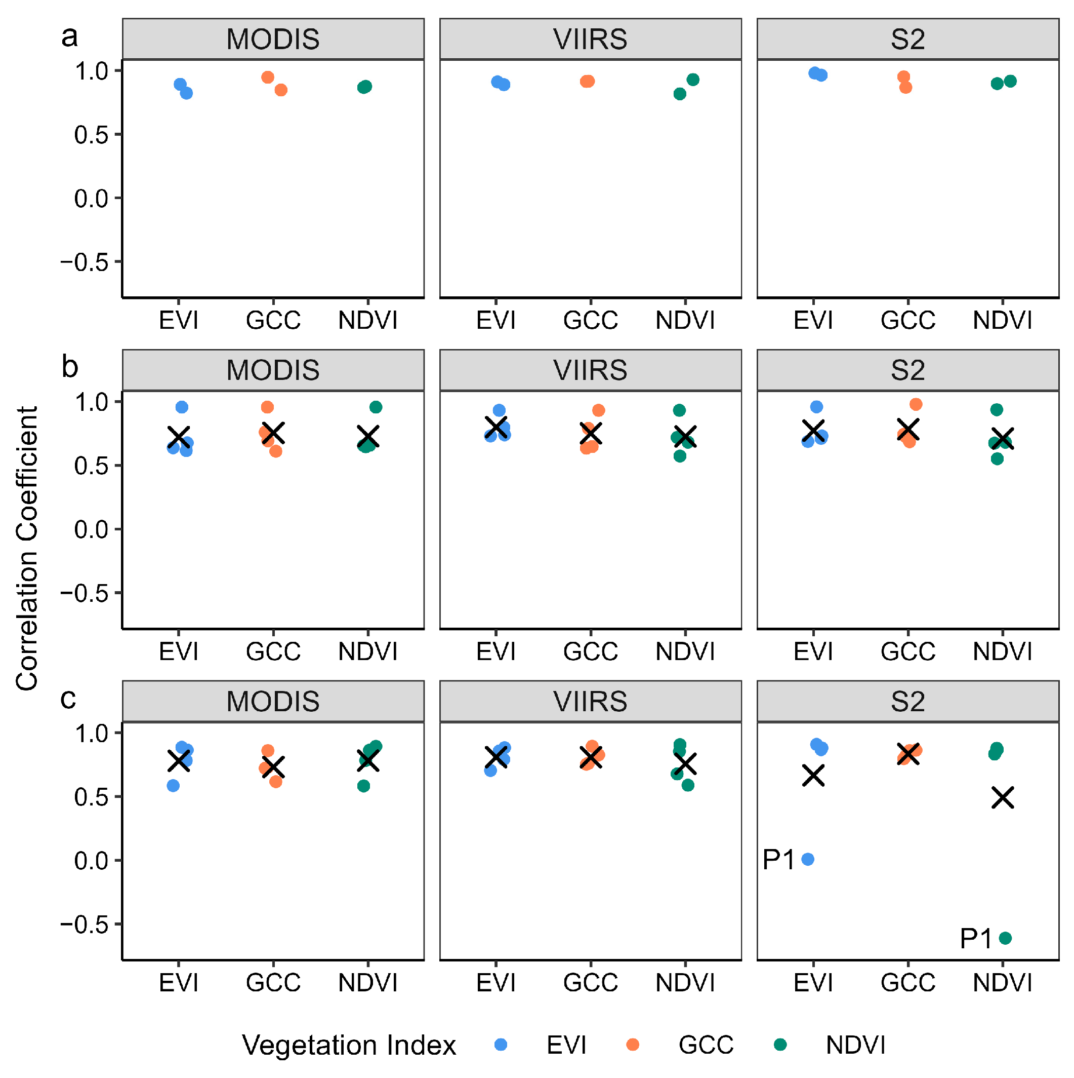
All satellites tracked the phenological patterns as documented by the ground-based phenocams well for at least one vegetation index. VIIRS and MODIS datasets were consistently highly correlated across vegetation indices. The highest correlations were observed for VIIRS-derived EVI and S2-derived GCC, followed by VIIRS-derived GCC, MODIS-derived GCC, and MODIS-derived NDVI (Figure 2, Figure 3 and Figure A1). The performance of each VI in tracking phenology varied across satellites.
Figure 2.
Time-series plots from plot W3, Ongava Game Reserve. Each row corresponds to a different satellite, and each column corresponds to a different vegetation index (GCC (Green Chromatic Coordinate) represented in orange, EVI (Enhanced Vegetation Index) represented in blue, NDVI (Normalised-Difference Vegetation Index) represented in green). The satellites shown are MODIS (Moderate Resolution Imaging Spectroradiometer), VIIRS (Visible Infrared Imaging Radiometer Suite), and S2 (Sentinel-2). See Figure A1 in Appendix A for time-series plots from all study plots.
Figure 3.
Graph of satellite-derived vegetation index correlation coefficients with Phenocam-GCC at 10 study plots over the 2022–2023 and 2023–2024 growing seasons. The datasets displayed are MODIS-EVI (mean = 0.74 ± 0.17), MODIS-GCC (mean = 0.78 ± 0.12), MODIS-NDVI (mean = 0.78 ± 0.15), VIIRS-EVI (mean = 0.83 ± 0.08), VIIRS-GCC (mean = 0.81 ± 0.11), VIIRS-NDVI (mean = 0.78 ± 0.14), S2-EVI (mean = 0.77 ± 0.29), S2-GCC (mean = 0.83 ± 0.10), and S2-NDVI (mean = 0.66 ± 0.47). Mean is displayed as a black cross mark for each dataset.
Satellite vegetation indices generally correlated best with ground phenology at Kilwa District and performed similarly at Bicuar National Park and Ongava Game Reserve, with more variability between sites for S2-derived EVI and NDVI datasets (Figure A3).
Visual inspection highlights the impact of data availability on satellite observations, with more discontinuous phenology time series derived from S2, with large periods without observations (Figure 2). MODIS had a greater number of observations in the study period and was more sensitive, showing greater intra-seasonal fluctuations than VIIRS and S2, but this was not associated with higher correlations with phenocams than VIIRS (Table A7).
3.1.2. Transition Date Estimate Comparison Between Ground Phenology Data and Satellite EO Products
MODIS and VIIRS datasets performed similarly in estimating transition dates. The bias for start-of-season (SOS) estimates was less than 5 days early for all MODIS and VIIRS datasets except for MODIS-derived EVI (Table 1). MODIS-derived end-of-season (EOS) estimates were biased from 7–11 days late, and VIIRS-derived EOS estimates were biased 19–21 days late. S2 did not have sufficient observation frequency to estimate SOS, POS, and LOS at all study plots, and estimated EOS dates had a bias of 19–30 days late for study plots in Bicuar National Park and Ongava Game Reserve. There were insufficient observations for Kilwa District EOS estimation.
Table 1.
Table containing the Bias, MAE, RMSE, and number of dates missing of each satellite-derived vegetation index transition date comparison with phenocam–GCC transition dates. See Table A6 for per-site errors.
All of the satellite datasets estimated a longer growing season than phenocams, with satellites typically detecting an earlier SOS and a later EOS. LOS estimates from phenocams ranged from 50 days at plot W6 in Ongava for the 2023–2024 growing season to 250 days at plot P1 in Ongava for the 2023–2024 growing season, with a mean LOS estimate of 121 days across all plots and growing seasons. Greater error and variability on average for EOS dates than SOS dates indicate a greater ability to identify the onset of the growing season from satellites than the end of season.
All datasets made the greatest errors in estimating POS (38–77 days RMSE). Whilst S2 datasets had insufficient observations for POS estimation, MODIS and VIIRS had similarly high POS estimate errors (Table 1). Only MODIS GCC and VIIRS EVI had an RMSE of 40 days or less. NDVI had greater errors in POS estimates in both MODIS and VIIRS than EVI or GCC. POS errors had no effect on LOS estimates, which are quantified as EOS minus SOS.
MODIS-derived NDVI, MODIS-derived GCC, and VIIRS-derived EVI were the most accurate for estimating SOS, and MODIS-derived EVI, MODIS-derived NDVI, and VIIRS-derived NDVI were most accurate for estimating EOS. Whilst MODIS-NDVI most accurately estimated LOS when both SOS and EOS estimates were available for a given season, MODIS-NDVI made large errors in POS estimates. Conversely, VIIRS-EVI was consistently accurate across all SOS, POS, EOS, and LOS.
3.1.3. Transition Date Sensitivity to Thresholds
The most accurate satellite–VI datasets varied across SOS and EOS thresholds, and all satellite–VI datasets had a positive average LOS bias for all SOS and EOS thresholds, except for MODIS-EVI in the 0.25 SOS threshold and 0.95 EOS threshold analysis. Across transition date thresholds, VIIRS NDVI was within the two most accurate datasets for 15 of the 16 SOS–EOS threshold combinations (see Table A5). Similarly, MODIS NDVI was within the two most accurate datasets for all SOS thresholds with EOS thresholds 0.90 and 0.95 and was only less accurate than more than three datasets for the 0.1 SOS threshold with a 0.80 and 0.85 EOS threshold. Additionally, VIIRS EVI was consistently within the four most accurate datasets for all SOS and EOS thresholds, and MODIS GCC was within the four most accurate datasets for 9 of 16 SOS–EOS threshold combinations.
3.2. Observation Frequency and Precipitation
The proportion of days with observations in each month declined significantly with total monthly precipitation (β = −0.001 ± 0.0001, p < 0.001). Satellite also had a significant effect, with significantly higher proportions of days with observations each month observed in MODIS compared to VIIRS (β = −0.236 ± 0.014, p < 0.001) and S2 (β = −0.707 ± 0.014, p < 0.001). Kilwa District had significantly lower proportions of days with observations each month than Ongava Game Reserve (β = −0.143 ± 0.020, p < 0.001), but there was no significant difference between proportions of days with observations each month in Ongava Game Reserve and Bicuar National Park (β = −0.014 ± 0.014, p = 0.307).
All months with no S2 observations occurred in the upper 50th percentile of total monthly precipitation months at the Kilwa District study location. The months with no MODIS observations were in the upper 75th percentile of total monthly precipitation months at the Kilwa District study location, and VIIRS did not have any months without observations.
3.3. Effect of Temporal Resampling of MODIS and VIIRS Satellite EO Products
Temporal resolution was more important for the accuracy of transition date estimation than time series correlation values. The temporally resampled MODIS- and VIIRS-derived vegetation indices showed little difference in correlations with ground phenology (Figure A3 and Table A7). Small reductions in correlations between MODIS- and VIIRS-derived vegetation indices and ground phenology are observed across all datasets except for MODIS-derived EVI, for which it showed a small increase. Transition date estimates typically showed greater RMSE and bias across temporally resampled MODIS- and VIIRS-derived vegetation indices, with greater RMSE differences observed for MODIS datasets than VIIRS (Table A8). Temporal resampling of MODIS and VIIRS datasets also led to insufficient data to estimate some SOS, LOS, and POS transition dates at some sites. Temporally resampled MODIS and VIIRS datasets maintained greater performance in transition date estimation than the S2 datasets. This suggests that S2’s missing data gaps spanning more than 1 calendar month are in part responsible for poor transition date estimation. Whilst S2-derived GCC was the strongest correlating dataset to ground phenology, S2-derived NDVI was the least correlated to ground phenology. S2-derived EVI was comparable but lower than most other datasets in its correlation coefficients with ground phenology. This demonstrates a difference in the quality of S2 compared to MODIS and VIIRS after temporal resampling, which varies with vegetation index.
4. Discussion
The challenges in accurate monitoring of vegetation phenology in African savannas, caused by heterogeneous phenologies within ecosystems and atmospheric interference, were more easily overcome in the moderate spatial resolution and high temporal resolution satellites (MODIS and VIIRS), than the high spatial resolution and low temporal resolution satellite (S2). MODIS and VIIRS vegetation indices closely tracked ground-based, phenocam phenology, with NDVI performing best for MODIS and EVI for VIIRS. S2 EVI and GCC were highly correlated with phenocam phenology but showed large errors in transition date estimation due, at least in part, to limited observations, particularly early in the growing season (See Figure 3). The accuracy of S2 in monitoring phenological temporal patterns was highly variable across study plots and the comparatively low effective temporal resolution of S2, with frequent missing observations, contributed to inaccurate monitoring of phenological transition dates in African savannas.
Overall, MODIS-derived NDVI provided the most accurate representation of temporal phenological patterns and transition dates. For both MODIS and VIIRS, satellite-derived GCC captured general trends but had larger errors in end-of-season estimates (See Table 1). Whilst VIIRS datasets were most highly correlated to phenocam phenology time series, the strongest correlations were not directly associated with accurate transition date estimates. Differences in phenology measurement accuracy between satellites were associated with differences in spectral sensitivities, viewing angles, temporal resolution, and spatial resolution. Differences in phenology measurement accuracy between VIs were associated with their distinct spectral emphases (e.g., green band versus red and near-infrared bands). The findings in this study support the application of MODIS and VIIRS for accurate monitoring of annual land-surface leaf phenological trends in African savannas, while intra-seasonal fluctuations were generally tracked less closely.
4.1. Association Between Phenology Measurement Accuracy and the Spectral Characteristics of Vegetation Indices and Satellite Sensors
Satellite-derived accuracy in tracking phenology was influenced by the sensitivity of satellite sensors to spectral wavelengths and the spectral composition of vegetation indices. Whilst growing season length was consistently overestimated across satellite datasets, driven by early start-of-season and late end-of-season estimates, the accuracy of temporal trends varied across satellites and vegetation indices (See Figure 3 and Table 1).
All of the satellite-derived VI time series showed a peak in values (POS) that was quite different from the POS of Gcc values in the phenocam time series. A peak in Gcc values occurs when the intensity of the green spectral band is highest relative to the red and blue bands. NDVI and EVI do not incorporate the green spectral band in their formulation, which could explain their mismatch with the Gcc POS [66]. In addition, the low accuracy of peak-of-season estimates in NDVI datasets may be influenced by unaccounted-for atmospheric conditions and a saturated detection limit during peak season [42,67]. Our results support evidence from tropical sites across a precipitation gradient that showed a reduction in NDVI sensitivity during peak season [41,68,69]. The satellite-derived POS in Gcc estimates were also very different from the phenocam-derived POS estimates, suggesting a more general challenge in consistently identifying the POS. For example, the lateral viewing angles of phenocams allow detection of greater leaf area than the nadir viewing angle of satellites, which is likely to support a wider detection capacity for leaf growth changes in phenocam measurements to which satellites may be less sensitive [58].
Overestimated growing seasons in satellite observations may reflect differences in observation angles, detection of photosynthetic activity, and impacts of temporal smoothing models. Within a patch of vegetation, phenocams typically observe greater leaf area than satellites due to their oblique viewing angle [21,58]. However, the larger overall field of view of satellite observations may result in a broader range of phenological timings observed in satellites, resulting in detection of earlier leaf growth and later senescence that are unobserved in the phenocam field of view [21,32,70]. Additionally, models applied to smoothing vegetation index time-series data have a significant impact on the tracking of phenology. Mean absolute deviations in start-of-season dates estimated from double logistic versus asymmetric Gaussian models were up to 3-to-4 weeks in dry deciduous vegetation in India, which was significantly reduced in other models [71].
The greater accuracy in start-of-season estimates than end-of-season estimates in this study reflects findings from dryland sites in the United States, in which this difference in accuracy was attributed to the more rapid change in leaf colour in the green-up phase than the senescence phase [21,72]. The consistency of earlier start-of-season estimates and later end-of-season estimates across vegetation indices highlights that overestimation of growing season length in satellites cannot be accounted for by differential detection of greenness and physiological leaf growth signals alone [41].
The high correlations between satellite GCC and phenocam phenology are in agreement with studies in semi-arid deciduous forests, savannas, and grasslands across the Americas, but the lower accuracy of satellite GCC end-of-season dates in this study does not match the high performance of GCC in other studies [30,42,73]. The low accuracy of end-of-season estimates in satellite-derived GCC datasets may suggest that the incorporation of NIR into NDVI and EVI, and the detection of physiological changes in leaf growth, support the detection of the end of season. Overall, NDVI was comparatively accurate in estimating the start, length, and end of growing season, suggesting good detection of leaf growth and senescence in African savanna vegetation. In summary, observed differences in the accuracy of vegetation indices are the result of differing spectral properties, further influenced by the spectral sensitivity of each sensor.
4.2. Association Between Phenology Measurement Accuracy and Temporal Resolution
Temporal resolution, determined by the satellite revisit frequency and the number of good-quality cloud-free observations, is a key characteristic of each satellite and likely to be driving some of the observed differences in accuracy of satellite measurements of phenology [27,74,75]. Almost daily observations from MODIS and VIIRS satellites, even after the removal of observations in the quality-filtering process, allowed for accurate transition dates compared to S2. Similarly, the high variability in temporal correlations in the S2 dataset were not observed in the MODIS and VIIRS datasets. The low proportion of days per month with observations by S2, particularly in high precipitation months, suggests high interference from atmospheric conditions and clouds affects the suitability of S2 for monitoring phenological transition dates across the African savanna sites. Periods of missing observations in the S2 dataset are particularly evident at the high-rainfall study plots in Kilwa District, Tanzania (see Figure 4 and Table A3). The association between low S2 accuracy in phenological monitoring and precipitation observed in this study reflects similar findings in croplands and freshwater ecosystems [74,75]. Additional studies have shown increasing uncertainties in phenological monitoring with decreasing temporal resolution, particularly when affected by missing data gaps associated with atmospheric conditions during the onset of the growing season [21,31,75].
Figure 4.
Total monthly precipitation (mm) and the proportion of days with observations for each calendar month by (a) MODIS, (b) VIIRS, and (c) S2 at the three study sites. Observations with a value greater than 0 are represented by a filled circle and observations with a value of 0 are represented by an unfilled circle. The linear model line of best fit is represented by black lines with confidence intervals represented in grey.
The proportion of days per month with observations was also associated with tracking of intraseasonal fluctuations in phenology, with MODIS documenting intraseasonal fluctuations most accurately and containing the highest proportion of days with observations (see Figure A3). Subtle seasonality patterns are challenging to detect due to masking from atmospheric and shadowing effects [70]. But the increased sensitivity of MODIS to intraseasonal fluctuations compared to VIIRS and S2 supports the robustness of previous studies measuring MODIS-derived phenological responses to intraseasonal variability in precipitation in Africa [76,77,78].
4.3. Association Between Phenology Measurement Accuracy and Spatial Resolution
Despite reported advantages of high spatial resolution for phenology monitoring, moderate spatial resolution satellites tracked phenology most accurately in this study, partially attributed to the aforementioned advantages of high temporal resolution and the phenocam observation scale in this study. The vegetation covered by a satellite pixel or phenocam monitoring area is determined by satellite pixel grid or phenocam installation design [22,34]. Studies in North American grasslands and savannas found that accuracy in phenology measurements increased with spatial resolution, attributed to the reduced influence of sub-pixel mixed vegetation on VIs [21,31,33,78]. Whilst spatial resolution is the same for VIIRS and MODIS, they can vary in their quantification of phenological patterns due to non-aligned pixel grids, including different vegetation in each pixel [37,79]. Phenological measurements from high spatial resolution satellites, such as S2 and Landsat, were more accurate than measurements from lower-resolution satellites in comparison to single phenocam phenology in semi-arid ecosystems in the northern hemisphere [21,31,33]. However, phenocam measurements in this study represent the average across three phenocams in each plot, installed to represent vegetation across a 100 m-by-100 m plot, monitoring a larger area of vegetation than a single camera. Consequently, phenocam observations in this study have a wider spatial coverage than single phenocam observations and may better represent the vegetation of the entire study plot. These plot-level multiple phenocam observations were most accurately measured by moderate spatial resolution satellites in this study, suggesting phenocam observations at the 1-hectare plot-level scale well with moderate spatial resolution satellites with pixels covering 25 hectares. Our findings highlight the value of multiple phenocam design for upscaling high spatiotemporal resolution phenocams using high coverage, moderate spatial resolution satellite datasets.
The difference in viewing angles between satellites and phenocams [80], in addition to VI sensitivity and temporal resolution, may explain S2 NDVI and EVI inaccuracy in tracking the phenology of plot P1 at the Ongava Game Reserve (Table A4c, Figure A1g). Whilst the dominance of bare ground in the localised area of plot P1 is likely minimised in the oblique viewing angle of phenocams, bare ground will remain dominant within the small S2 pixel size. The larger pixel size of MODIS and VIIRS includes more surrounding vegetation that is not bare ground. This artifact is supported by observations of dominant land-use cover differing between phenocams and satellites in a savanna in the United States, with increased representation of bare ground in satellites [21,81].
5. Conclusions
In this study, we have supported the accuracy of MODIS and VIIRS phenological measurements in African savannas. In particular, the MODIS-derived NDVI, VIIRS-derived EVI, and MODIS-derived GCC showed the greatest accuracy in monitoring phenology across African savanna sites, with high accuracy in temporal trend monitoring and transition date estimation. S2’s sensitivity to atmospheric interference reduced this satellite’s ability to monitor phenological transition dates across the African savanna sites in this study. Despite accurate tracking of temporal trends, the Green Chromatic Coordinate (GCC) performed less well in estimating transition dates than the vegetation indices that incorporated NIR reflectance (NDVI and EVI). Our findings support the potential robustness of research applying satellite measurements for investigating phenological patterns and controls in African savannas. While our phenocam sample and coverage were restricted, the multiple phenocam design indicates a strong relationship in this study between phenology time series derived from phenocam and moderate resolution satellites, suggesting an opportunity for upscaling small scale, high resolution phenocam datasets over larger spatial and temporal scales. Accurate monitoring of phenology in African savannas is crucial for identifying long-term trends associated with changing environmental conditions, understanding interactions between savanna vegetation and the atmosphere, and effective monitoring of ecosystem health in these highly productive regions.
Author Contributions
Conceptualization, F.C.O., T.R.B., K.G.D., and D.M.R.; methodology, F.C.O., T.R.B., K.G.D., D.M.R., L.P.C.M., and B.A.; software, L.P.C.M., B.A., and D.M.R.; formal analysis, F.C.O.; investigation, F.C.O.; data curation, F.C.O., D.M.R., K.G.D., V.D.C., F.M.G., M.C., G.I.K.U., and M.S.; writing—original draft preparation, F.C.O.; writing—review and editing, T.R.B., K.G.D., D.M.R., L.P.C.M., V.D.C., C.M.R., and J.L.G.; supervision, T.R.B. and K.G.D. All authors have read and agreed to the published version of the manuscript.
Funding
This research was funded by a Natural Environment Research Council SENSE Centre for Doctoral Training PhD studentship at the University of Leeds (NE/T00939X/1), the Natural Environment Research Council-Funded SECO Project (NE/T01279X/1), and the Natural Environment Research Council-Funded PhenoChange Project (NE/X002993/1). L.P.C.M., D.M.R. and B.A. are funded by FAPESP—São Paulo Research Foundation (grants 2021/10639-5, 2022/02323-0); L.P.C.M. receives a Research Productivity fellowship from the National Council for Scientific and Technological Development-CNPq (grant 306563/2022-3).
Data Availability Statement
The data presented in this study are available on request from the corresponding author due to privacy reasons.
Acknowledgments
We thank the collaborating institutions for the support and permissions to work at the research sites.
Conflicts of Interest
The authors declare no conflicts of interest. The funders had no role in the design of the study; in the collection, analyses, or interpretation of data; in the writing of the manuscript; or in the decision to publish the results.
Abbreviations
The following abbreviations are used in this manuscript:
| MODIS | Moderate Resolution Imaging Spectroradiometer |
| VIIRS | Visible Infrared Imaging Radiometer Suite |
| S2 | Sentinel-2 |
| PC | Phenocam |
| SOS | Start of season |
| POS | Peak of season |
| EOS | End of season |
| LOS | Length of season |
| NDVI | Normalised Difference Vegetation Index |
| EVI | Enhanced Vegetation Index |
| GCC | Green Chromatic Coordinate |
| MAE | Mean Absolute Error |
| RMSE | Root Mean Squared Error |
| SD | Standard Deviation |
| DOY | Day of Year |
| MAP | Mean Annual Precipitation |
| STV | SOS Threshold Value |
| ETV | EOS Threshold Value |
Appendix A
Table A1.
Table showing camera details and dates installed for each study plot.
Table A2.
A table showing the number of days in the 700-day study period in which an observation was available after quality filtering in each dataset.
Table A3.
Table showing plots where transition dates were excluded due to insufficient data for each dataset during the study period.
Table A4.
(a) Table showing a phenocam image, satellite image (with camera locations displayed in yellow), and coordinates at each study plot in Kilwa District. (b) Table showing a phenocam image, satellite image (with camera locations displayed in blue), and coordinates at each study plot in Bicuar National Park. (c) Table showing a phenocam image, satellite image (with camera locations displayed in red), and coordinates at each study plot in Ongava Game Reserve.
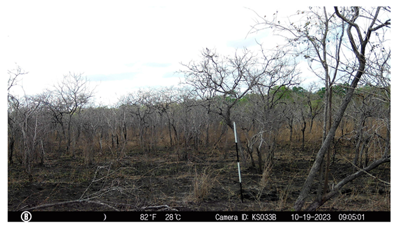
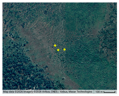
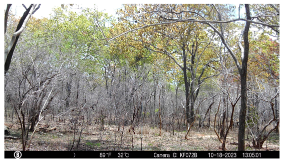
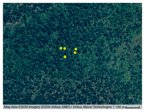
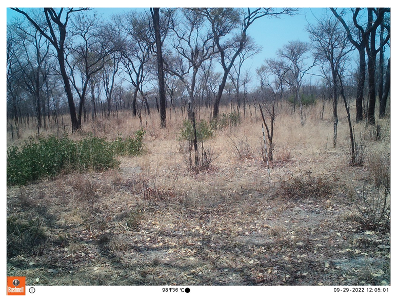
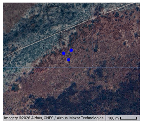
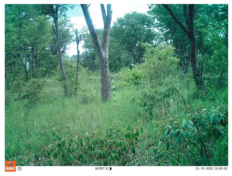
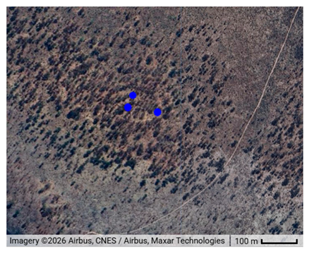
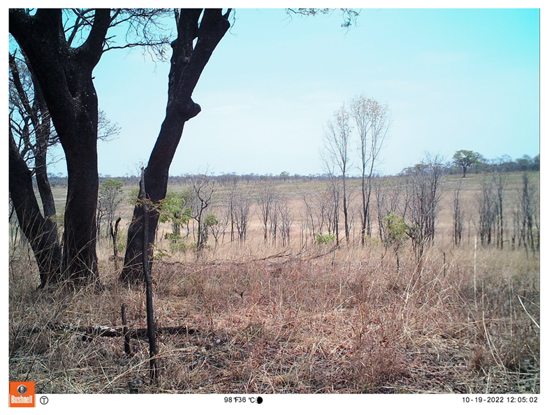
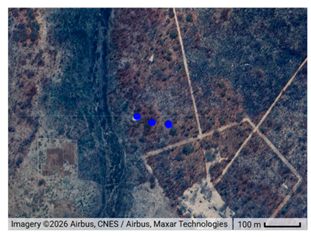
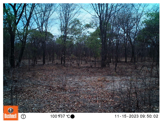
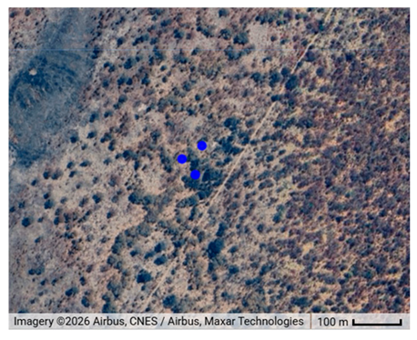
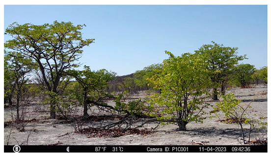
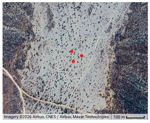
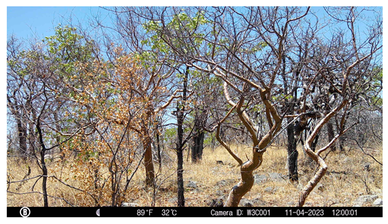
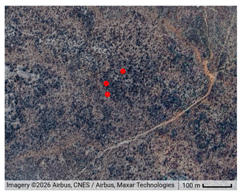
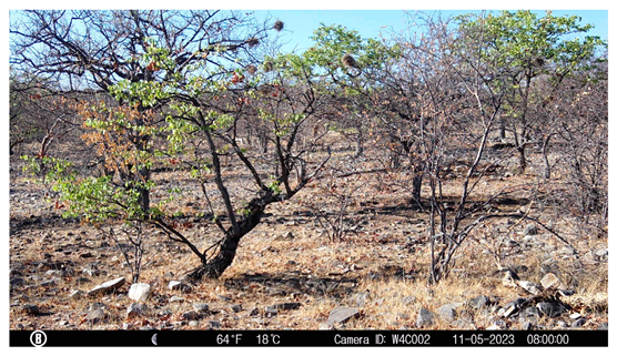
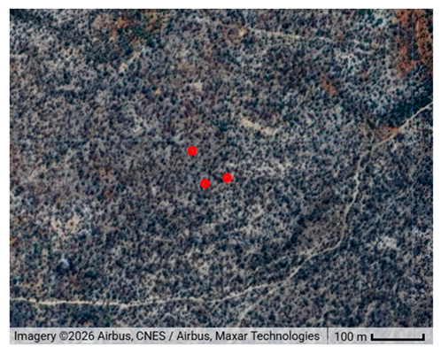
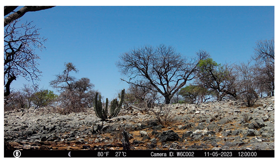
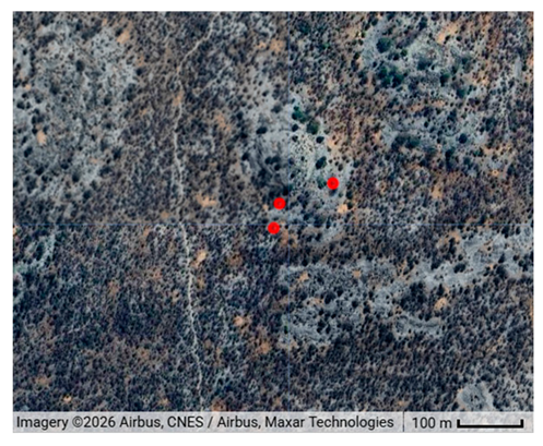
Table A5.
A table of the four lowest mean RMSE satellite-derived VI datasets across SOS and EOS transition dates for all combinations of SOS and EOS thresholds. The rankings displayed in this table are intended to visualise the similarities between transition date accuracy outcomes of the threshold scenarios and not a definitive ranking of performance. The applied thresholds in the main analysis are visualised in bold italic font.
Figure A1.
(a) Time-series plots from plot S03, Kilwa District. Each row corresponds to a different satellite, and each column corresponds to a different vegetation index (GCC represented in orange, EVI represented in blue, NDVI represented in green). (b) Time-series plots from plot F07, Kilwa District. Each row corresponds to a different satellite, and each column corresponds to a different vegetation index (GCC represented in orange, EVI represented in blue, NDVI represented in green). (c) Time-series plots from plot P2, Bicuar National Park. Each row corresponds to a different satellite, and each column corresponds to a different vegetation index (GCC represented in orange, EVI represented in blue, NDVI represented in green). (d) Time-series plots from plot P9, Bicuar National Park. Each row corresponds to a different satellite, and each column corresponds to a different vegetation index (GCC represented in orange, EVI represented in blue, NDVI represented in green). (e) Time-series plots from plot P10, Bicuar National Park. Each row corresponds to a different satellite, and each column corresponds to a different vegetation index (GCC represented in orange, EVI represented in blue, NDVI represented in green). (f) Time-series plots from plot P12, Bicuar National Park. Each row corresponds to a different satellite, and each column corresponds to a different vegetation index (GCC represented in orange, EVI represented in blue, NDVI represented in green). (g) Time-series plots from plot P1, Ongava Game Reserve. Each row corresponds to a different satellite, and each column corresponds to a different vegetation index (GCC represented in orange, EVI represented in blue, NDVI represented in green). (h) Time-series plots from plot W3, Ongava Game Reserve. Each row corresponds to a different satellite, and each column corresponds to a different vegetation index (GCC represented in orange, EVI represented in blue, NDVI represented in green). This figure is identical to Figure 2 in the main text. (i) Time-series plots from plot W4, Ongava Game Reserve. Each row corresponds to a different satellite, and each column corresponds to a different vegetation index (GCC represented in orange, EVI represented in blue, NDVI represented in green). (j) Time-series plots from plot W6, Ongava Game Reserve. Each row corresponds to a different satellite, and each column corresponds to a different vegetation index (GCC represented in orange, EVI represented in blue, NDVI represented in green).
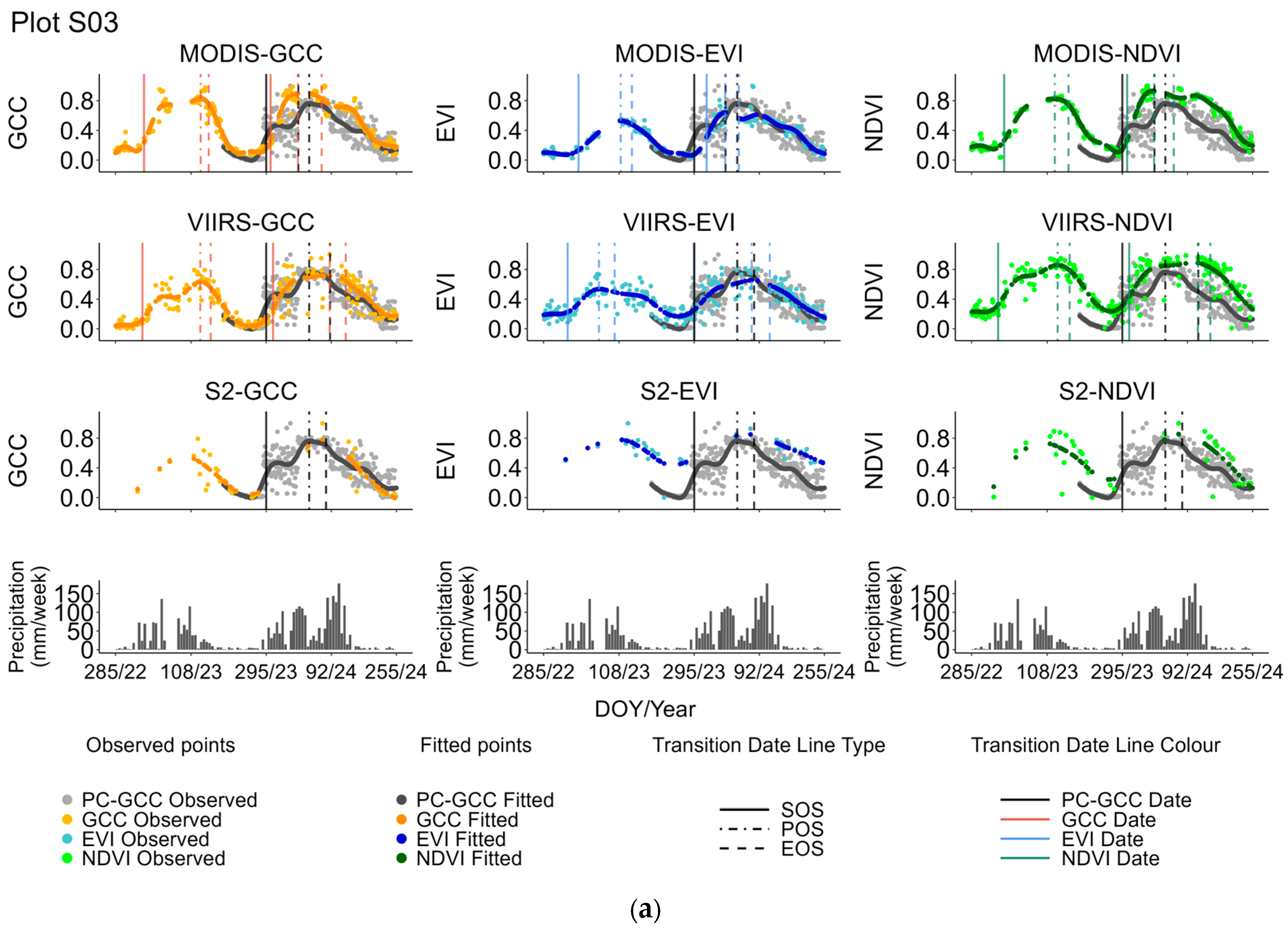
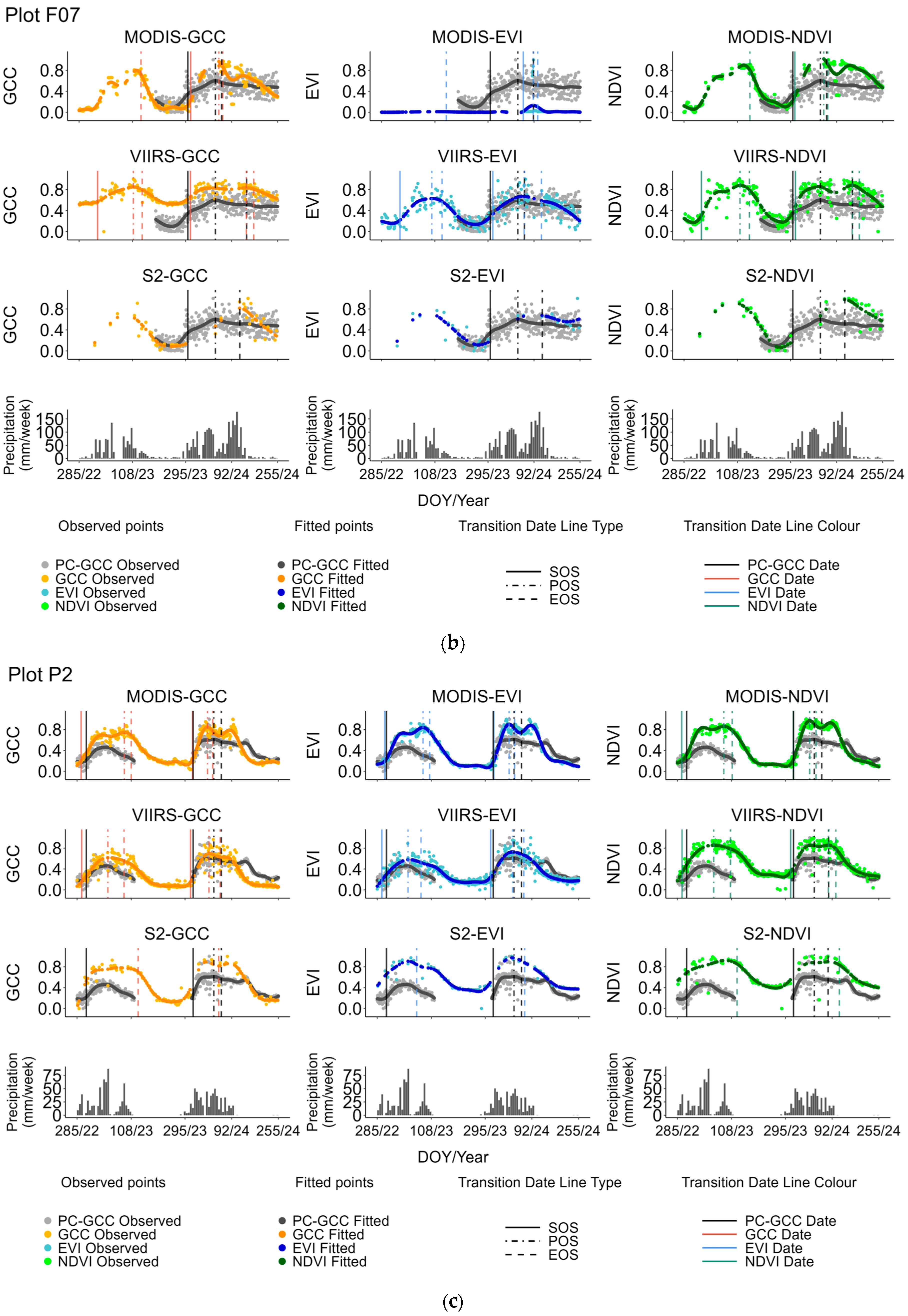
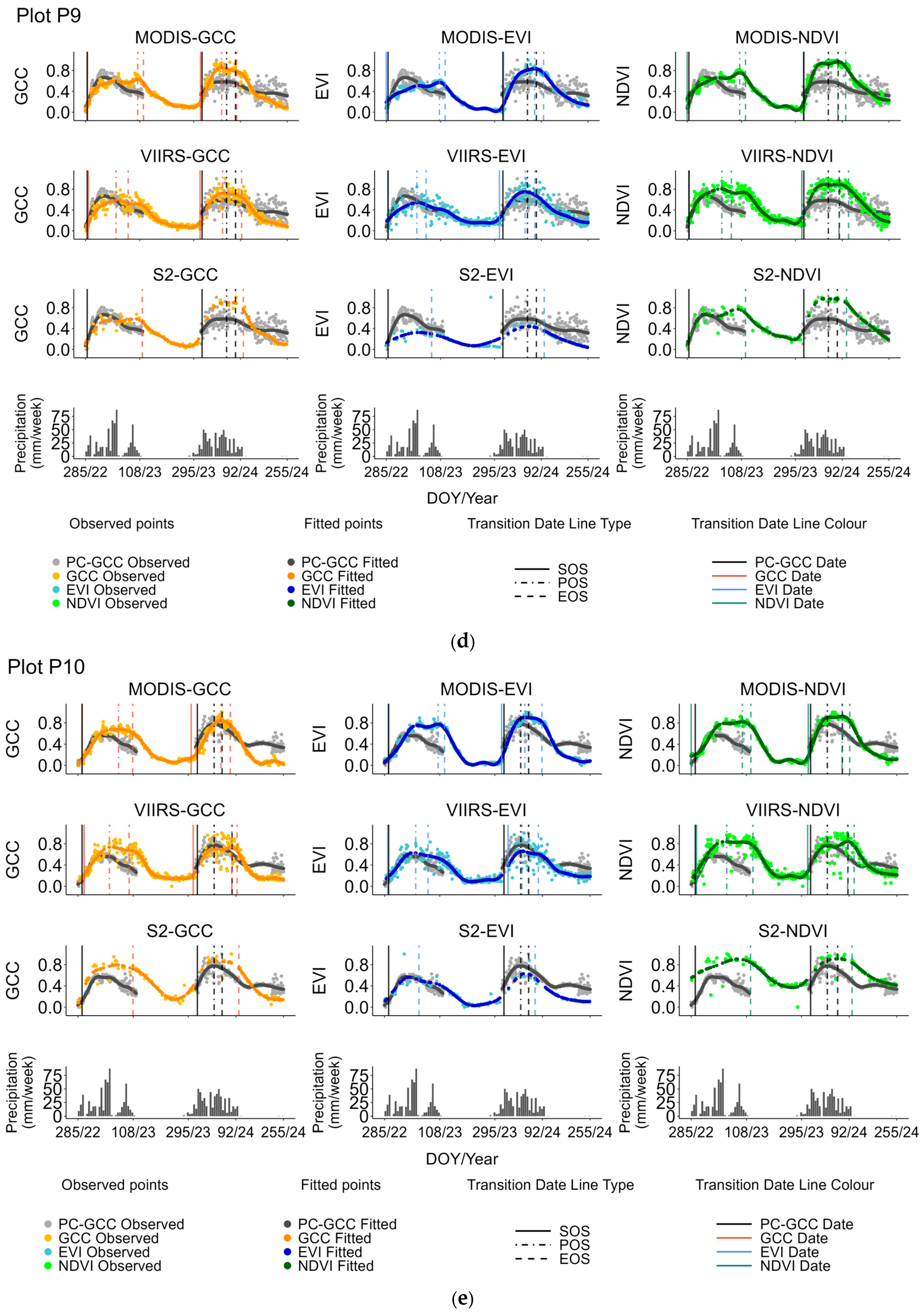
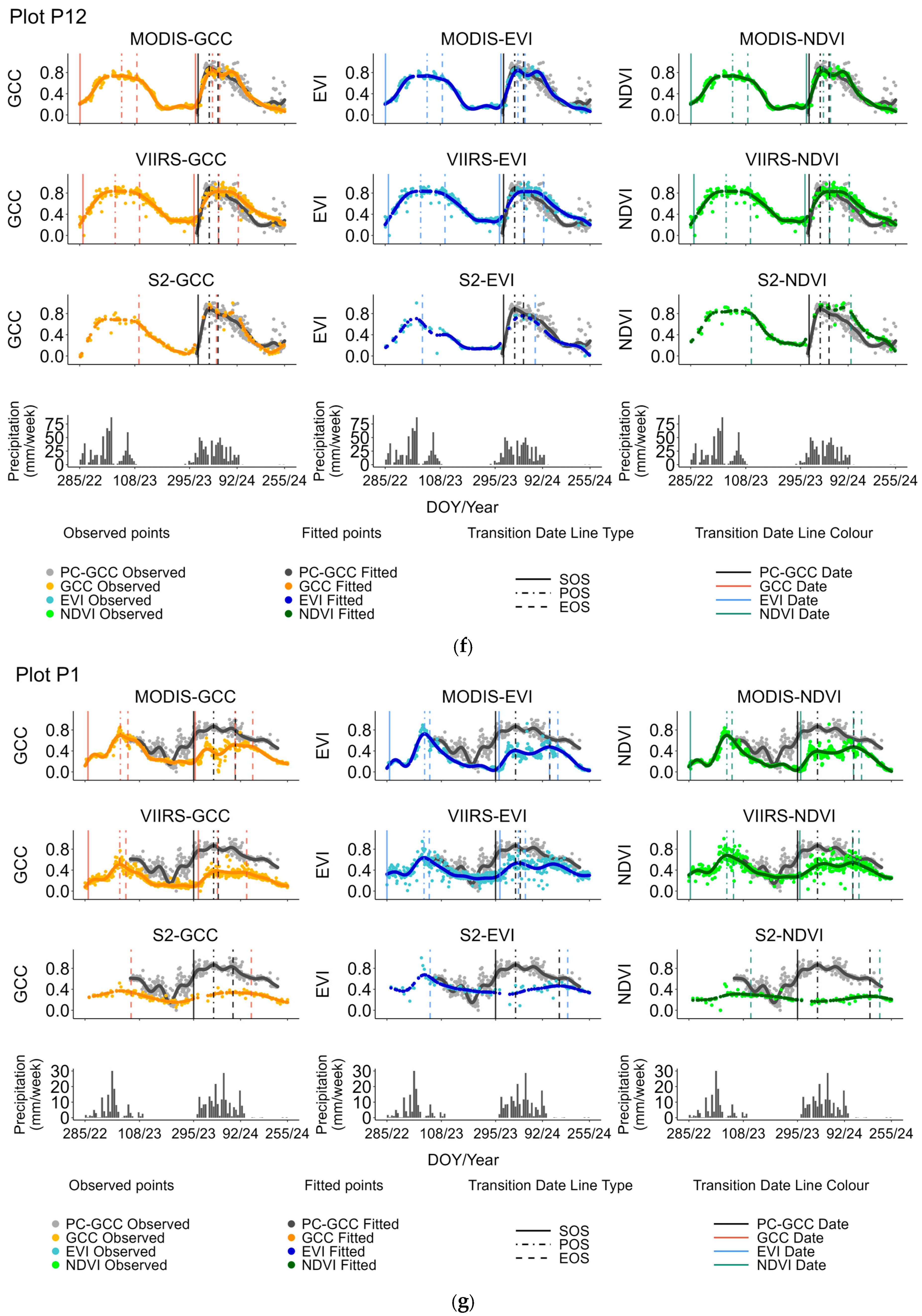
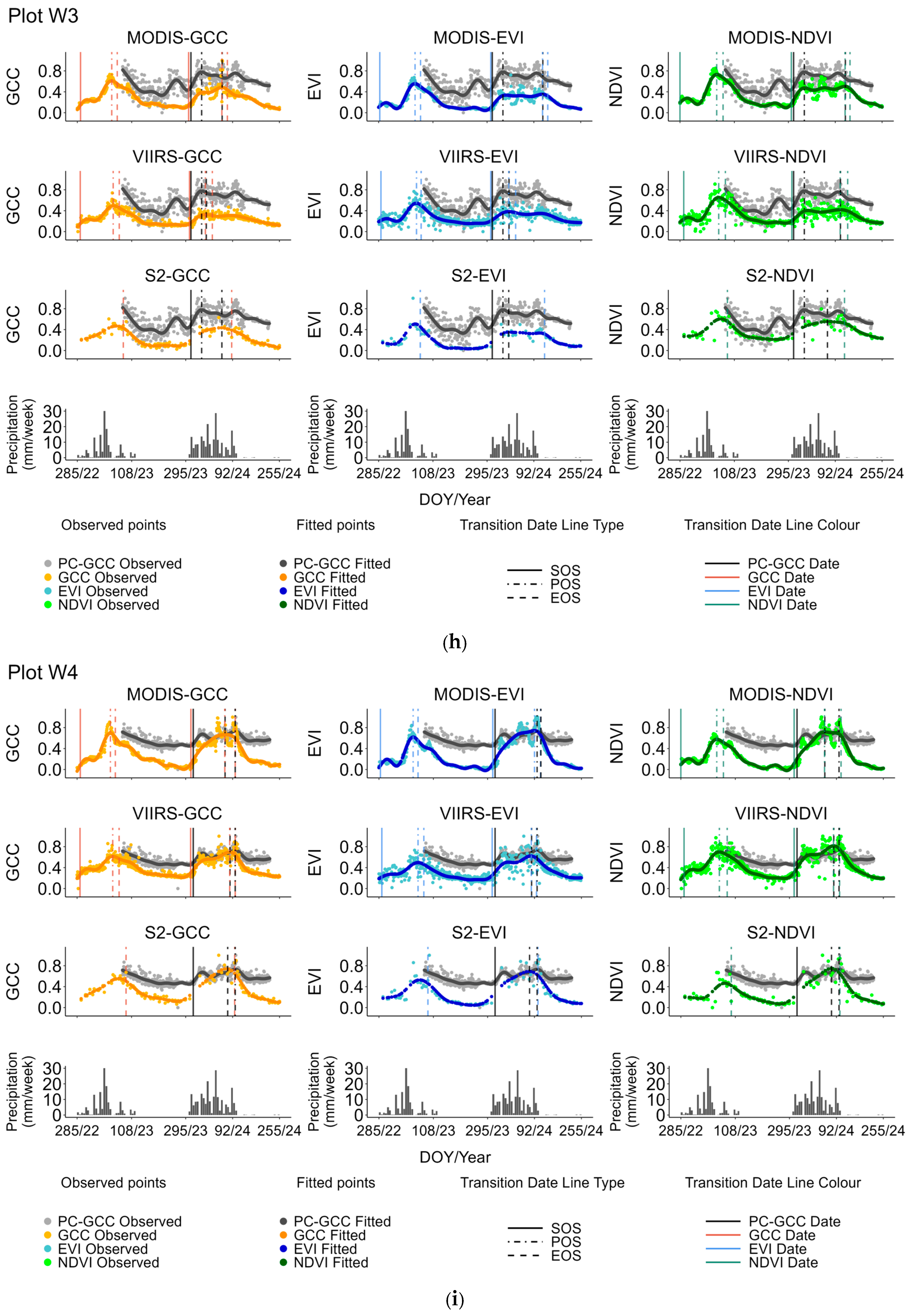
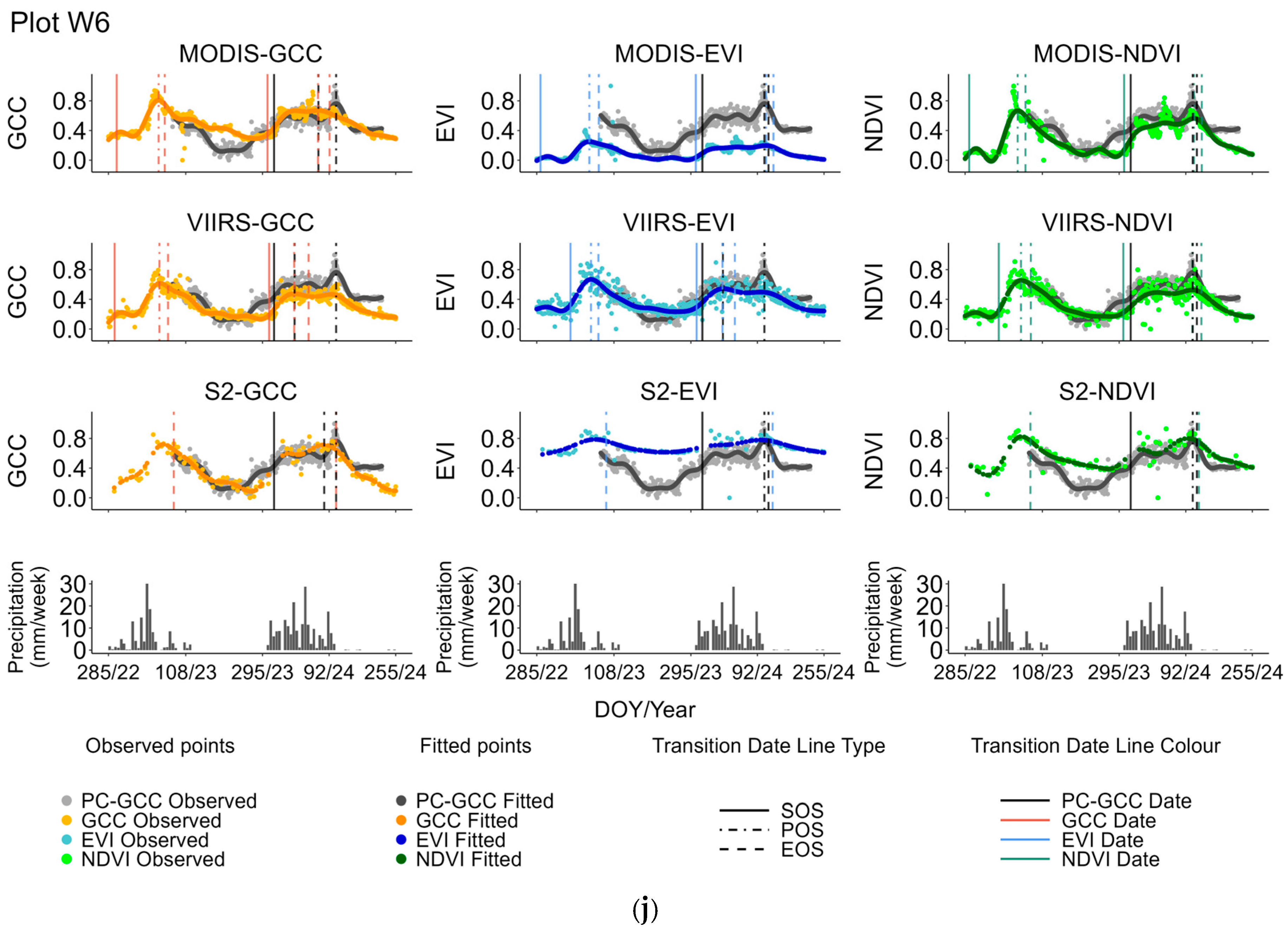
Table A6.
Table containing the Bias, MAE, RMSE, and number of NA dates of each satellite-derived vegetation index transition date comparison with phenocam–GCC transition dates at the study sites in Bicuar National Park, Angola, Ongava Game Reserve, Namibia, and Kilwa District, Tanzania.
Figure A2.
Graph of satellite-derived vegetation index correlation coefficients with Phenocam–GCC at 10 study plots by site ((a). Kilwa, (b). Bicuar, (c). Ongava) over the 2022–2023 growing season and 2023–2024 growing season. The datasets displayed are MODIS-EVI, MODIS-GCC, MODIS-NDVI, VIIRS-EVI, VIIRS-GCC, VIIRS-NDVI, S2-EVI, S2-GCC, S2-NDVI. Mean is displayed as a black cross mark for each dataset. Mean and standard deviation of each dataset shown in Table A5).
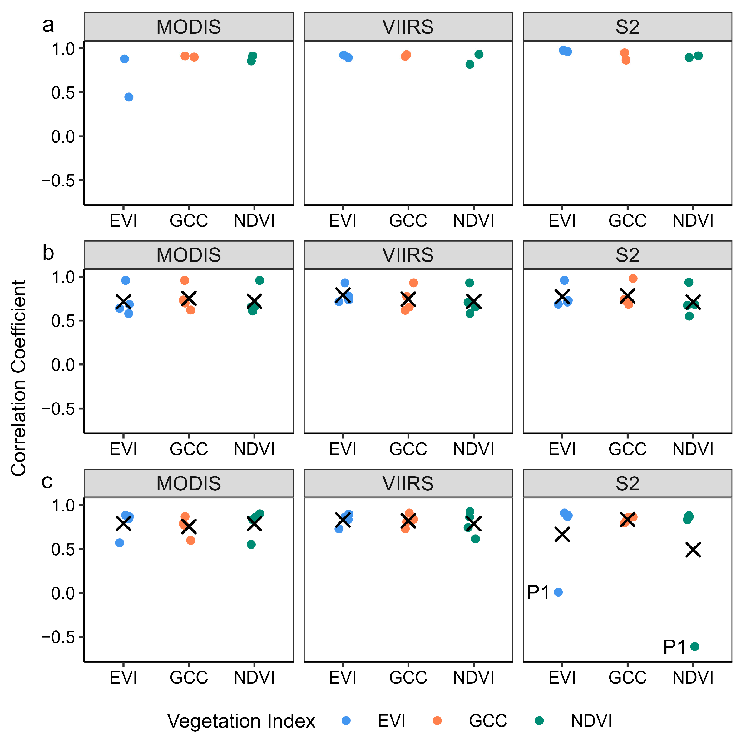
Figure A3.
Graph of temporally resampled satellite-derived vegetation index correlation coefficients with Phenocam–GCC at 10 study plots over the 2022–2023 growing season and 2023–2024 growing season. The datasets displayed are MODIS-EVI (mean = 0.77 ± 0.13), MODIS-GCC (mean = 0.77 ± 0.12), MODIS-NDVI (mean = 0.78 ± 0.13), VIIRS-EVI (mean = 0.82 ± 0.08), VIIRS-GCC (mean = 0.81 ± 0.11), VIIRS-NDVI (mean = 0.77 ± 0.14), S2-EVI (mean = 0.77 ± 0.29), S2-GCC (mean = 0.83 ± 0.10), S2-NDVI (mean = 0.66 ± 0.47). Mean is displayed as a black cross mark for each dataset.
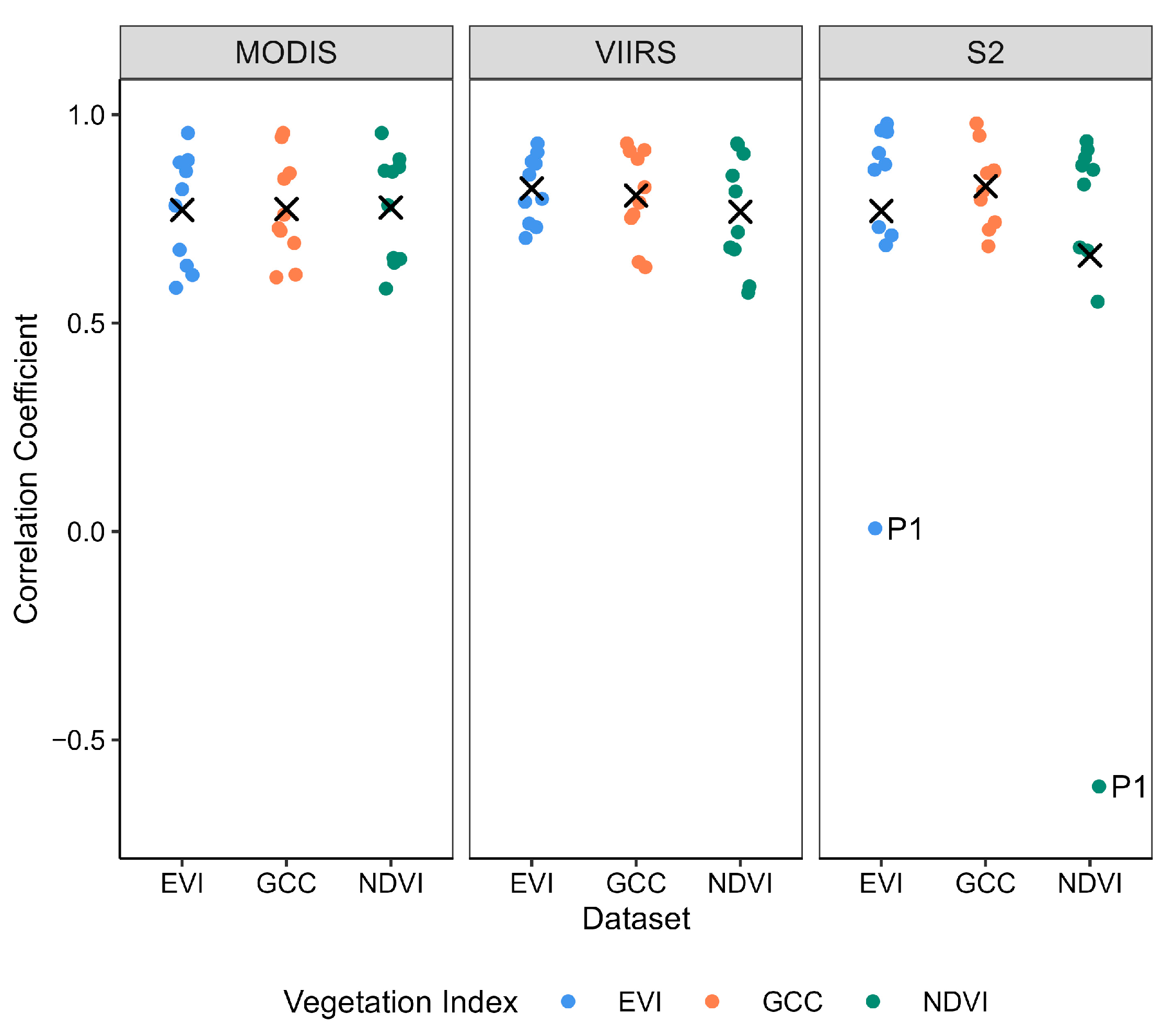
Table A7.
Satellite EO product vegetation index correlations by site in source temporal resolution and resampled temporal resolution.
Table A8.
Table containing the Bias, MAE, RMSE, and percentage of dates missing of each satellite-derived vegetation index transition date comparison with phenocam-GCC transition dates, with MODIS and VIIRS datasets resampled to the temporal resolution of S2.
Figure A4.
Graph of temporally resampled satellite-derived vegetation index correlation coefficients with Phenocam–GCC at 10 study plots by site ((a). Kilwa, (b). Bicuar, (c). Ongava) over the 2022–2023 growing season and 2023–2024 growing season. The datasets displayed are MODIS-EVI, MODIS-GCC, MODIS-NDVI, VIIRS-EVI, VIIRS-GCC, VIIRS-NDVI, S2-EVI, S2-GCC, S2-NDVI. Mean is displayed as a black cross mark for each dataset. Mean and standard deviation of each dataset shown in Table A6).
References
- Noormets, A. Phenology of Ecosystem Processes: Applications in Global Change Research; Springer: New York, NY, USA, 2009. [Google Scholar] [CrossRef] [Scilit]
- Inouye, D.W. Climate change and phenology. WIREs Clim. Change 2022, 13, e764. [Google Scholar] [CrossRef] [Scilit]
- Poulter, B.; Frank, D.; Ciais, P.; Myneni, R.B.; Andela, N.; Bi, J.; Broquet, G.; Canadell, J.; Chevallier, F.; Liu, Y.; et al. Contribution of semi-arid ecosystems to interannual variability of the global carbon cycle. Nature 2014, 509, 600–603. [Google Scholar] [CrossRef] [Scilit] [PubMed]
- Kikuzawa, K. Leaf phenology as an optimal strategy for carbon gain in plants. Can. J. Bot. 1995, 73, 158–163. [Google Scholar] [CrossRef] [Scilit]
- Linderholm, H.W. Growing season changes in the last century. Agric. For. Meteorol. 2006, 137, 1–14. [Google Scholar] [CrossRef] [Scilit]
- Chen, S.; Fu, Y.; Hao, F.; Li, X.; Zhou, S.; Liu, C.; Tang, J. Vegetation phenology and its ecohydrological implications from individual to global scales. Geogr. Sustain. 2022, 3, 334–338. [Google Scholar] [CrossRef] [Scilit]
- Adole, T.; Dash, J.; Atkinson, P. A systematic review of vegetation phenology in Africa. Ecol. Inform. 2016, 34, 117–128. [Google Scholar] [CrossRef] [Scilit]
- Alberton, B.; Torres, R.; Canciana, L.; Borgesa, B.; Almeida, J.; Mariano, G.; Santos, J.; Morellato, L. Introducing digital cameras to monitor plant phenology in the tropics: Applications for conservation. Perspect. Ecol. Conserv. 2017, 15, 82–90. [Google Scholar] [CrossRef] [Scilit]
- Bush, E.; Bunnefeld, N.; Dimoto, E.; Dikangadissi, J.-T.; Jeffery, K.; Tutin, C.; White, L.; Abernethy, K.A. Towards effective monitoring of tropical phenology: Maximizing returns and reducing uncertainty in long-term studies. Biotropica 2018, 50, 455–464. [Google Scholar] [CrossRef] [Scilit]
- Tang, J.; Körner, C.; Muraoka, H.; Piao, S.; Shen, M.; Thackeray, S.; Yang, X. Emerging opportunities and challenges in phenology: A review. Ecosphere 2016, 7, e01436. [Google Scholar] [CrossRef] [Scilit]
- Alberton, B.; Torres, R.; Silva, T.; Rocha, H.; Moura, M.; Morrellato, L. Leafing Patterns and Drivers across Seasonally Dry Tropical Communities. Remote Sens. 2019, 11, 2267. [Google Scholar] [CrossRef] [Scilit]
- Ramos, D.; Andrade, J.; Alberton, B.; Moura, M.; Domingues, T.; Neves, N.; Lima, J.; Souza, R.; Souza, E.; Silva, J.; et al. Multiscale phenology of seasonally dry tropical forests in an aridity gradient. Front. Environ. Sci. 2023, 11, 1275844. [Google Scholar] [CrossRef] [Scilit]
- Maphanga, T. The use of modified and unmodified digital cameras to monitor small-scale Savannah Rangeland vegetation. J. Rangel. Sci. 2025, 15, 1–8. [Google Scholar] [CrossRef]
- Studer, S.; Stöckli, R.; Appenzeller, C.; Vidale, P.L. A comparative study of satellite and ground-based phenology. Int. J. Biometeorol. 2007, 51, 405–414. [Google Scholar] [CrossRef] [Scilit] [PubMed]
- Guan, K.; Wood, E.; Medvigy, D.; Kimball, J.; Pan, M.; Caylor, K.; Sheffield, J. Terrestrial hydrological controls on land surface phenology of African savannas and woodlands. J. Geophys. Res. Biogeosci. 2014, 119, 1652–1669. [Google Scholar] [CrossRef] [Scilit]
- Adole, T.; Dash, J.; Atkinson, P.M. Large-scale prerain vegetation green-up across Africa. Glob. Change Biol. 2018, 24, 4054–4068. [Google Scholar] [CrossRef] [Scilit] [PubMed]
- Song, G.; Wang, J.; Zhao, Y.; Yang, D.; Lee, C.K.F.; Guo, Z.; Detto, M.; Alberton, B.; Morellato, P.; Nelson, B.W.; et al. Scale matters: Spatial resolution impacts tropical leaf phenology characterized by multi-source satellite remote sensing with an ecological-constrained deep learning model. Remote Sens. Environ. 2024, 304, 114027. [Google Scholar] [CrossRef] [Scilit]
- Archibald, S.; Scholes, R. Leaf green-up in a semi-arid African savanna-separating tree and grass responses to environmental cues. J. Veg. Sci. 2007, 18, 583–594. [Google Scholar] [CrossRef] [Scilit]
- Ryan, C.M.; Williams, M.; Grace, J.; Woollen, E.; Lehmann, C.E.R. Pre-rain green-up is ubiquitous across southern tropical Africa: Implications for temporal niche separation and model representation. New Phytol. 2017, 213, 625–633. [Google Scholar] [CrossRef] [Scilit] [PubMed]
- Godlee, J.; Ryan, C.; Siampale, A.; Dexter, K. Tree species diversity drives the land surface phenology of seasonally dry tropical woodlands. J. Ecol. 2024, 112, 1978–1991. [Google Scholar] [CrossRef] [Scilit]
- Yan, D.; Scott, R.L.; Moore, D.J.P.; Biederman, J.A.; Smith, W.K. Understanding the relationship between vegetation greenness and productivity across dryland ecosystems through the integration of PhenoCam, satellite, and eddy covariance data. Remote Sens. Environ. 2019, 223, 50–62. [Google Scholar] [CrossRef] [Scilit]
- Richardson, A.; Hufkens, K.; Milliman, T.; Frolking, S. Intercomparison of phenological transition dates derived from the PhenoCam Dataset V1.0 and MODIS satellite remote sensing. Sci. Rep. 2018, 8, 5679. [Google Scholar] [CrossRef] [Scilit] [PubMed]
- Higgins, S.; Delgado-Cartay, M.; February, E.; Combrink, H. Is there a temporal niche separation in the leaf phenology of savanna trees and grasses? J. Biogeogr. 2011, 38, 2165–2175. [Google Scholar] [CrossRef] [Scilit]
- Walker, J.J.; de Beurs, K.M.; Wynne, R.H.; Gao, F. Evaluation of Landsat and MODIS data fusion products for analysis of dryland forest phenology. Remote Sens. Environ. 2012, 117, 381–393. [Google Scholar] [CrossRef] [Scilit]
- Phiri, D.; Simwanda, M.; Salekin, S.; Nyirenda, V.R.; Murayama, Y.; Ranagalage, M. Sentinel-2 Data for Land Cover/Use Mapping: A Review. Remote Sens. 2020, 12, 2291. [Google Scholar] [CrossRef] [Scilit]
- Kaszta, Z.; Van De Kerchove, R.; Ramoelo, A.; Cho, M.A.; Madonsela, S.; Mathieu, R.; Wolff, E. Seasonal Separation of African Savanna Components Using Worldview-2 Imagery: A Comparison of Pixel-and Object-Based Approaches and Selected Classification Algorithms. Remote Sens. 2016, 8, 763. [Google Scholar] [CrossRef] [Scilit]
- Misra, G.; Cawkwell, F.; Wingler, A. Status of Phenological Research Using Sentinel-2 Data: A Review. Remote Sens. 2020, 12, 2760. [Google Scholar] [CrossRef] [Scilit]
- Marchant, R. Understanding complexity in savannas: Climate, biodiversity and people. Curr. Opin. Environ. Sustain. 2010, 2, 101–108. [Google Scholar] [CrossRef] [Scilit]
- Ryan, C.; Williams, M.; Hill, T.; Grace, J.; Woodhouse, I. Assessing the Phenology of Southern Tropical Africa: A Comparison of Hemispherical Photography, Scatterometry, and Optical/NIR Remote Sensing. IEEE Trans. Geosci. Remote Sens. 2014, 52, 519–528. [Google Scholar] [CrossRef] [Scilit]
- Koolen, S.P.; Godlee, J.L.; Alberton, B.; Ramos, D.M.; Moura, M.S.B.; Morellato, L.P.C.; Dexter, K.G. The Coexistence of Trees, Shrubs, and Grasses Creates a Complex Picture of Land Surface Phenology in Dry Tropical Ecosystems. Remote Sens. 2025, 17, 2883. [Google Scholar] [CrossRef] [Scilit]
- Liu, Y.; Hill, M.; Zhang, X.; Wang, Z.; Richardson, A.; Hufkens, K.; Filippa, G.; Baldocchi, D.; Ma, S.; Verfaillie Schaaf, C. Using data from Landsat, MODIS, VIIRS and PhenoCams to monitor the phenology of California oak/grass savanna and open grassland across spatial scales. Agric. For. Meteorol. 2017, 237–238, 311–325. [Google Scholar] [CrossRef] [Scilit]
- Browning, D.; Karl, J.; Morin, D.; Richardson, A.; Tweedie, C. Phenocams Bridge the Gap between Field and Satellite Observations in an Arid Grassland Ecosystem. Remote Sens. 2017, 9, 1071. [Google Scholar] [CrossRef] [Scilit]
- Zhang, X.; Wang, J.; Gao, F.; Liu, Y.; Schaaf, C.; Friedl, M.; Yu, Y.; Jayavelu, S.; Gray, J.; Liu, L.; et al. Exploration of scaling effects on coarse resolution land surface phenology. Remote Sens. Environ. 2017, 190, 318–330. [Google Scholar] [CrossRef] [Scilit]
- Skakun, S.; Justice, C.; Vermote, E.; Roger, J. Transitioning from MODIS to VIIRS: An analysis of inter-consistency of NDVI data sets for agricultural monitoring. Int. J. Remote Sens. 2018, 39, 971–992. [Google Scholar] [CrossRef] [Scilit] [PubMed]
- Walker, B.H.; Ludwig, D.; Holling, C.S.; Peterman, R.M. Stability of Semi-Arid Savanna Grazing Systems. J. Ecol. 1981, 69, 473–498. [Google Scholar] [CrossRef] [Scilit]
- Scholes, R.J.; Archer, S.R. Tree-Grass Interactions in Savannas. Annu. Rev. Ecol. Syst. 1997, 28, 517–544. [Google Scholar] [CrossRef] [Scilit]
- Chidumayo, E.N. Climate and Phenology of Savanna Vegetation in Southern Africa. J. Veg. Sci. 2001, 12, 347–354. [Google Scholar] [CrossRef] [Scilit]
- Whitecross, M.A.; Witkowski, E.T.F.; Archibald, S. Savanna tree-grass interactions: A phenological investigation of green-up in relation to water availability over three seasons. S. Afr. J. Bot. 2017, 108, 29–40. [Google Scholar] [CrossRef] [Scilit]
- Wigley-Coetsee, C.; Staver, A. Grass community responses to drought in an African savanna. Afr. J. Range Forage Sci. 2020, 37, 43–52. [Google Scholar] [CrossRef] [Scilit]
- Burke, M.; Rundquist, B. Scaling Phenocam GCC, NDVI, and EVI2 with Harmonized Landsat-Sentinel using Gaussian Processes. Agric. For. Meteorol. 2021, 300, 108316. [Google Scholar] [CrossRef] [Scilit]
- Huete, A.; Didan, K.; Miura, T.; Rodriguez, E.P.; Gao, X.; Ferreira, L.G. Overview of the radiometric and biophysical performance of the MODIS vegetation indices. Remote Sens. Environ. 2002, 83, 195–213. [Google Scholar] [CrossRef] [Scilit]
- Zhang, J.; Xiao, J.; Tong, X.; Zhang, J.; Li, J.; Lin, P.; Yu, P.; Meng, P. Comparing the performance of phenocam GCC, MODIS GCC, and MODIS EVI for retrieving vegetation phenology and estimating gross primary production. Ecol. Indic. 2024, 166, 112251. [Google Scholar] [CrossRef] [Scilit]
- Hill, M.J. Vegetation index suites as indicators of vegetation state in grassland and savanna: An analysis with simulated SENTINEL 2 data for a North American transect. Remote Sens. Environ. 2013, 137, 94–111. [Google Scholar] [CrossRef] [Scilit]
- De Cauwer, V.; Colace, M.; Mendelsohn, J.; Antonio, T.; Van Der Waal, C. A rangeland management-oriented approach to map dry savanna—Woodland mosaics. Int. J. Appl. Earth Obs. Geoinf. 2024, 134, 1569–8432. [Google Scholar] [CrossRef] [Scilit]
- Godlee, J.; Gonçalves, F.; Tchamba, J.; Chisingui, A.; Muledi, J.; Shutcha, M.; Ryan, C.; Brade, T.; Dexter, K. Diversity and Structure of an Arid Woodland in Southwest Angola, with Comparison to the Wider Miombo Ecoregion. Diversity 2020, 12, 140. [Google Scholar] [CrossRef] [Scilit]
- McNicol, I.; Ryan, C.; Dexter, K.; Ball, S.; Williams, M. Aboveground Carbon Storage and Its Links to Stand Structure, Tree Diversity and Floristic Composition in South-Eastern Tanzania. Ecosystems 2018, 21, 740–754. [Google Scholar] [CrossRef] [Scilit] [PubMed]
- Ramos, D.; Gonçalves, R.; Moura, M.; Espírito-Santo, M.; Coutinho, Í.; De Cauwer, V.; Alberton, B.; Muledi, J.; Ryan, C.; Cachissapa, M.; et al. The PhenoChange network protocol for monitoring leaf phenology in tropical dry ecosystems using phenocameras. Methods Ecol. Evol. 2026, early view. [Google Scholar] [CrossRef] [Scilit]
- Sonnentag, O.; Hufkens, K.; Teshera-Sterne, C.; Young, A.; Friedl, M.; Braswell, B.; Milliman, T.; O’Keefe, J.; Richardson, A. Digital repeat photography for phenological research in forest ecosystems. Agric. For. Meteorol. 2012, 22, 159–177. [Google Scholar] [CrossRef] [Scilit]
- van Buuren, S.; Groothuis-Oudshoorn, K. mice: Multivariate Imputation by Chained Equations in R. J. Stat. Softw. 2011, 45, 1–67. [Google Scholar] [CrossRef] [Scilit]
- R Core Team. R: A Language and Environment for Statistical Computing version 4.4.1; R Foundation for Statistical Computing: Vienna, Austria, 2024; Available online: https://www.R-project.org/ (accessed on 1 July 2026).
- Vermote, E.; Franch, B.; Claverie, M. VIIRS/NPP Surface Reflectance Daily L2G Global 1km and 500m SIN Grid V002 [Data Set]; NASA EOSDIS Land Processes Distributed Active Archive Center: Sioux Falls, SD, USA, 2023. [Google Scholar]
- Funk, C.; Peterson, P.; Landsfeld, M.; Pedreros, D.; Verdin, J.; Shukla, S.; Husak, G.; Rowland, J.; Harrison, L.; Hoell, A.; et al. The climate hazards infrared precipitation with stations-a new environmental record for monitoring extremes. Sci. Data 2015, 2, 150066. [Google Scholar] [CrossRef] [Scilit] [PubMed]
- Gorelick, N.; Hancher, M.; Dixon, M.; Ilyushchenko, S.; Thau, D.; Moore, R. Google Earth Engine: Planetary-scale geospatial analysis for everyone. Remote Sens. Environ. 2017, 202, 18–27. [Google Scholar] [CrossRef] [Scilit]
- Bannari, A.; Morin, D.; Bonn, F.; Huete, A.R. A review of vegetation indices. Remote Sens. Rev. 1995, 13, 95–120. [Google Scholar] [CrossRef] [Scilit]
- Joint Nature Conservation Committee. JNCC Sentinel-2 indices Analysis Ready Data (ARD) Enhanced Vegetation Index (EVI); NERC EDS Centre for Environmental Data Analysis: Oxfordshire, UK, 2022; Available online: https://catalogue.ceda.ac.uk/uuid/102909b1d169469f85c099a6f1686bad (accessed on 24 October 2025).
- NASA. Earth Data: Sentinel-2: MSI [Dataset]. 2026. Available online: https://www.earthdata.nasa.gov/data/instruments/sentinel-2-msi (accessed on 24 October 2025).
- NASA. LAADS DAAC: Terra & Aqua Moderate Resolution Imaging Spectroradiometer (MODIS) [Dataset]. 2026. Available online: https://ladsweb.modaps.eosdis.nasa.gov/missions-and-measurements/modis/ (accessed on 24 October 2025).
- NASA. LAADS DAAC: Visible Infrared Imaging Radiometer Suite (VIIRS) [Dataset]. 2026. Available online: https://ladsweb.modaps.eosdis.nasa.gov/missions-and-measurements/viirs/ (accessed on 24 October 2025).
- Moulin, S.; Kergoat, L.; Viovy, N.; Dedieu, G. Global-Scale Assessment of Vegetation Phenology Using NOAA/AVHRR Satellite Measurements. J. Clim. 1997, 10, 1154–1170. [Google Scholar] [CrossRef] [Scilit]
- Zhang, X.; Friedl, M.A.; Schaaf, C.B.; Strahler, A.H.; Hodges, C.F.; Gao, F.; Reed, B.C.; Huete, A. Monitoring vegetation phenology using MODIS. Remote Sens. Environ. 2003, 84, 471–475. [Google Scholar] [CrossRef] [Scilit]
- Friedl, M.; Gray, J.; Sulla-Menashe, D. MODIS/Terra+Aqua Land Cover Dynamics Yearly L3 Global 500m SIN Grid V061 [Dataset]; NASA Land Processes Distributed Active Archive Center: Sioux Falls, SD, USA, 2022. [Google Scholar] [CrossRef]
- Wu, Z.; Fun, Y.; Crowther, T.; Renner, S.; Vitasse, Y.; Mo, L.; Zou, Y.; Mirzagholi, L.; Li, M.; Rebindaine, D.; et al. Carry-over effects between spring and autumn phenology differ among the world’s biomes. Natl. Sci. Rev. 2026, 13, nwag082. [Google Scholar] [CrossRef] [Scilit] [PubMed]
- Akinyemi, F.; Graw, V. Two decades of agricultural drought impacts: Remote sensing insights into vegetation productivity and phenological change in semi-arid Botswana. Environ. Monit. Assess. 2026, 198, 188. [Google Scholar] [CrossRef] [Scilit] [PubMed]
- Zhang, J.; Tong, X.; Zhang, J.; Meng, P.; Li, J.; Liu, P. Dynamics of phenology and its response to climatic variables in a warm-temperate mixed plantation. For. Ecol. Manag. 2021, 483, 118785. [Google Scholar] [CrossRef] [Scilit]
- Morellato, L.P.C.; Camargo, M.G.G.; D’Eça Neves, F.F.; Luize, B.G.; Mantovani, A.; Hudson, I.L. The Influence of Sampling Method, Sample Size, and Frequency of Observations on Plant Phenological Patterns and Interpretation in Tropical Forest Trees. In Phenological Research; Hudson, I., Keatley, M., Eds.; Springer: Dordrecht, The Netherlands, 2010. [Google Scholar] [CrossRef] [Scilit]
- Pettorelli, N.; Vik, J.O.; Mysterud, A.; Gaillard, J.-M.; Tucker, C.J.; Stenseth, N.C. Using the satellite-derived NDVI to assess ecological responses to environmental change. Trends Ecol. Evol. 2005, 20, 9. [Google Scholar] [CrossRef] [Scilit] [PubMed]
- Rankine, C.; Sanchez-Azofeifa, G.A.; Guzman, A.; Espirito-Santo, M.M.; Sharp, I. Comparing MODIS and near-surface vegetation indexes for monitoring tropical dry forest phenology along a successional gradient using optical phenology towers. Environ. Res. Lett. 2017, 12, 105007. [Google Scholar] [CrossRef] [Scilit]
- Tian, F.; Brandt, M.; Liu, Y.Y.; Veger, A.; Tagesson, T.; Diouf, A.A.; Rasmussen, K.; Mbow, C.; Wang, Y.; Fensholt, R. Remote sensing of vegetation dynamics in drylands. Remote Sens. Environ. 2016, 177, 265–276. [Google Scholar] [CrossRef] [Scilit]
- Tong, X.; Tian, F.; Brandt, M.; Liu, Y.; Zhang, W.; Fensholt, R. Trends of land surface phenology derived from passive microwave and optical remote sensing systems and associated drivers across the dry tropics 1992–2012. Remote Sens. Environ. 2019, 232, 111307. [Google Scholar] [CrossRef] [Scilit]
- Xiong, X.; Butler, J. MODIS and VIIRS Calibration History and Future Outlook. Remote Sens. 2020, 12, 2523. [Google Scholar] [CrossRef] [Scilit]
- Brown, L.A.; Dash, J.; Ogutua, B.O.; Richardson, A.D. On the relationship between continuous measures of canopy greenness derived using near-surface remote sensing and satellite-derived vegetation products. Agric. For. Meteorol. 2017, 247, 280–292. [Google Scholar] [CrossRef] [Scilit]
- Atkinson, P.; Jeganathan, C.; Dash, J.; Atzberger, C. Inter-comparison of four models for smoothing satellite sensor time-series data to estimate vegetation phenology. Remote Sens. Environ. 2012, 123, 400–417. [Google Scholar] [CrossRef] [Scilit]
- Cui, T.; Martz, L.; Zhao, L.; Guo, X. Investigating the impact of the temporal resolution of MODIS data on measured phenology in the prairie grasslands. GISci. Remote Sens. 2020, 57, 395–410. [Google Scholar] [CrossRef] [Scilit]
- Duncan, J.; Dash, J.; Atkinson, P. The potential of satellite-observed crop phenology to enhance yield gap assessments in smallholder landscapes. Front. Environ. Sci. Sec. Environ. Inform. Remote Sens. 2015, 3, 56. [Google Scholar] [CrossRef] [Scilit]
- Villa, P.; Pinardi, M.; Bolpagni, R.; Gillier, J.; Zinke, P.; Nedelcuţ, F.; Bresciani, M. Assessing macrophyte seasonal dynamics using dense time series of medium resolution satellite data. Remote Sens. Environ. 2018, 216, 230–244. [Google Scholar] [CrossRef] [Scilit]
- Zhang, X.; Friedl, M.A.; Schaaf, C.B.; Strahler, A.H. Monitoring the response of vegetation phenology to precipitation in Africa by coupling MODIS and TRMM instruments. J. Geophys. Res. 2005, 110, D12103. [Google Scholar] [CrossRef] [Scilit]
- Funk, C.C.; Brown, M.E. Intra-seasonal NDVI change projections in semi-arid Africa. Remote Sens. Environ. 2006, 101, 249–256. [Google Scholar] [CrossRef] [Scilit]
- Cissé, S.; Eymard, L.; Ottlé, C.; Ndione, J.A.; Gaye, A.T.; Pinsard, F. Rainfall intra-seasonal variability and vegetation growth in the Ferlo basin (Senegal). Remote Sens. 2016, 8, 66. [Google Scholar] [CrossRef] [Scilit]
- Tran, K.H.; Zhang, X.; Ye, Y.; Henebry, G.M.; Friedl, M.A.; Shen, Y.; Liu, Y.; An, S.; Gao, S. An insight into long-term continuity in global land surface phenology: A comparative analysis of MODIS and VIIRS products. Remote Sens. Environ. 2025, 331, 115024. [Google Scholar] [CrossRef] [Scilit]
- Thapa, S.; Millan, V.; Eklundh, L. Assessing Forest Phenology: A Multi-Scale Comparison of Near-Surface (UAV, Spectral Reflectance Sensor, PhenoCam) and Satellite (MODIS, Sentinel-2). Remote Sens. 2021, 13, 1597. [Google Scholar] [CrossRef] [Scilit]
- Keenan, T.F.; Darby, B.; Felts, E.; Sonnentag, O.; Friedl, M.A.; Hufkens, K.; O’Keefe, J.; Klosterman, S.; Munger, J.W.; Toomey, M.; et al. Tracking forest phenology and seasonal physiology using digital repeat photography: A critical assessment. Ecol. Appl. 2014, 24, 1478–1489. [Google Scholar] [CrossRef] [Scilit] [PubMed]
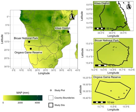
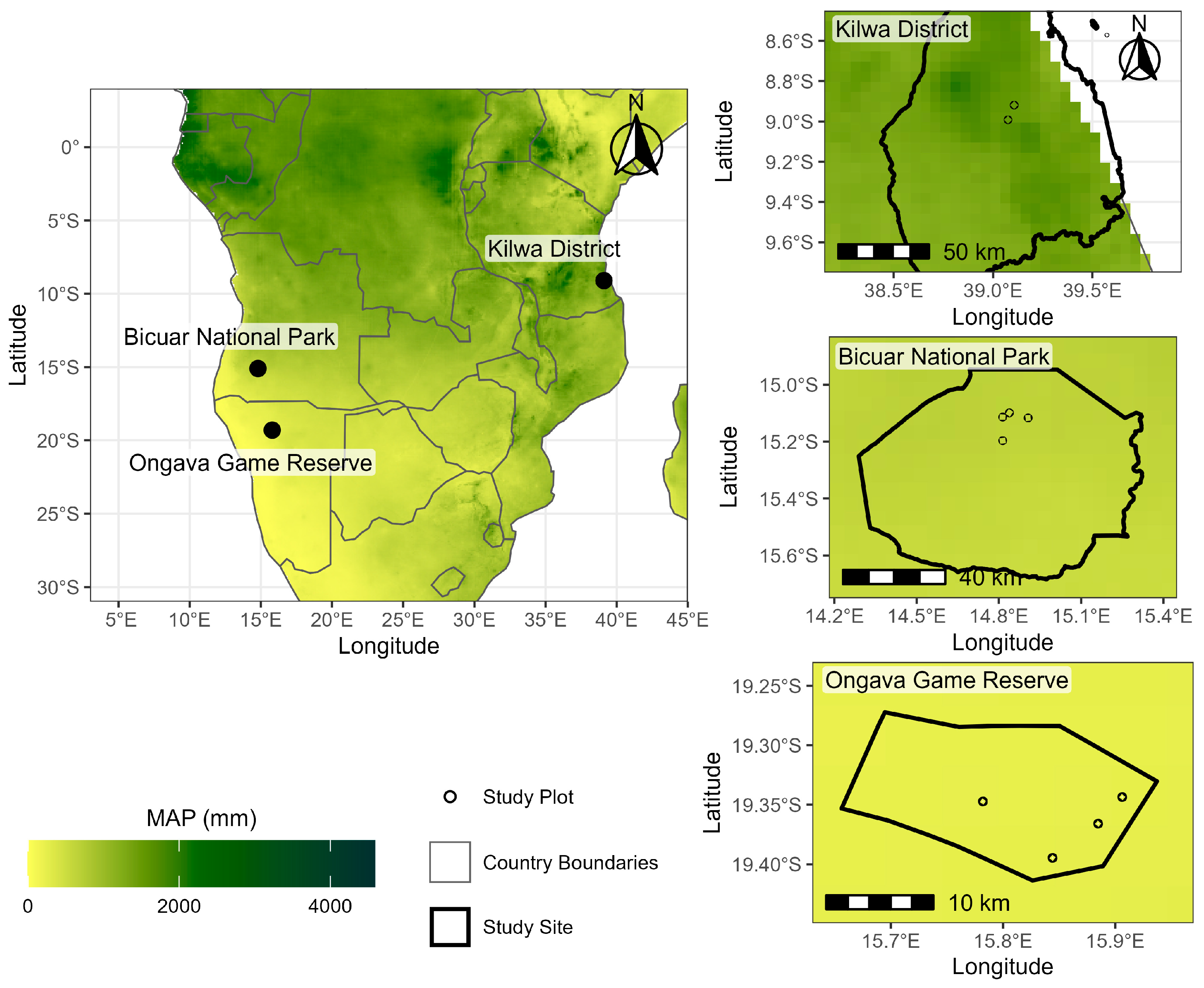
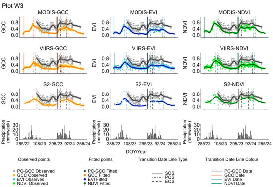
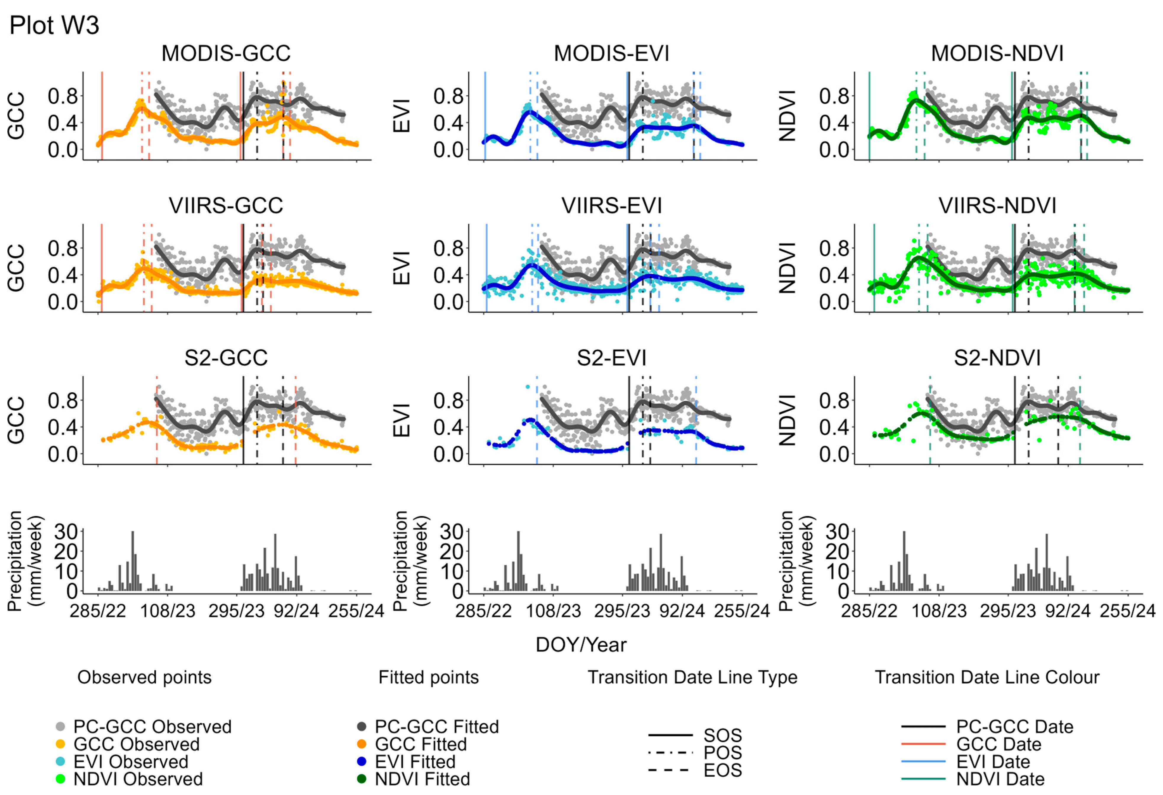
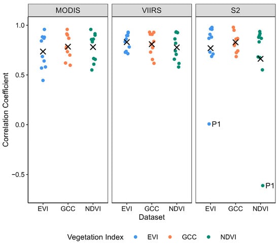
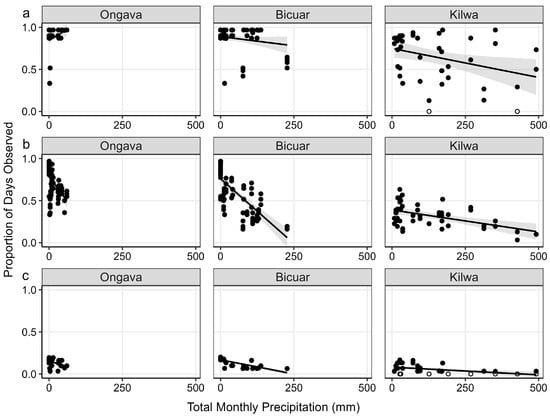
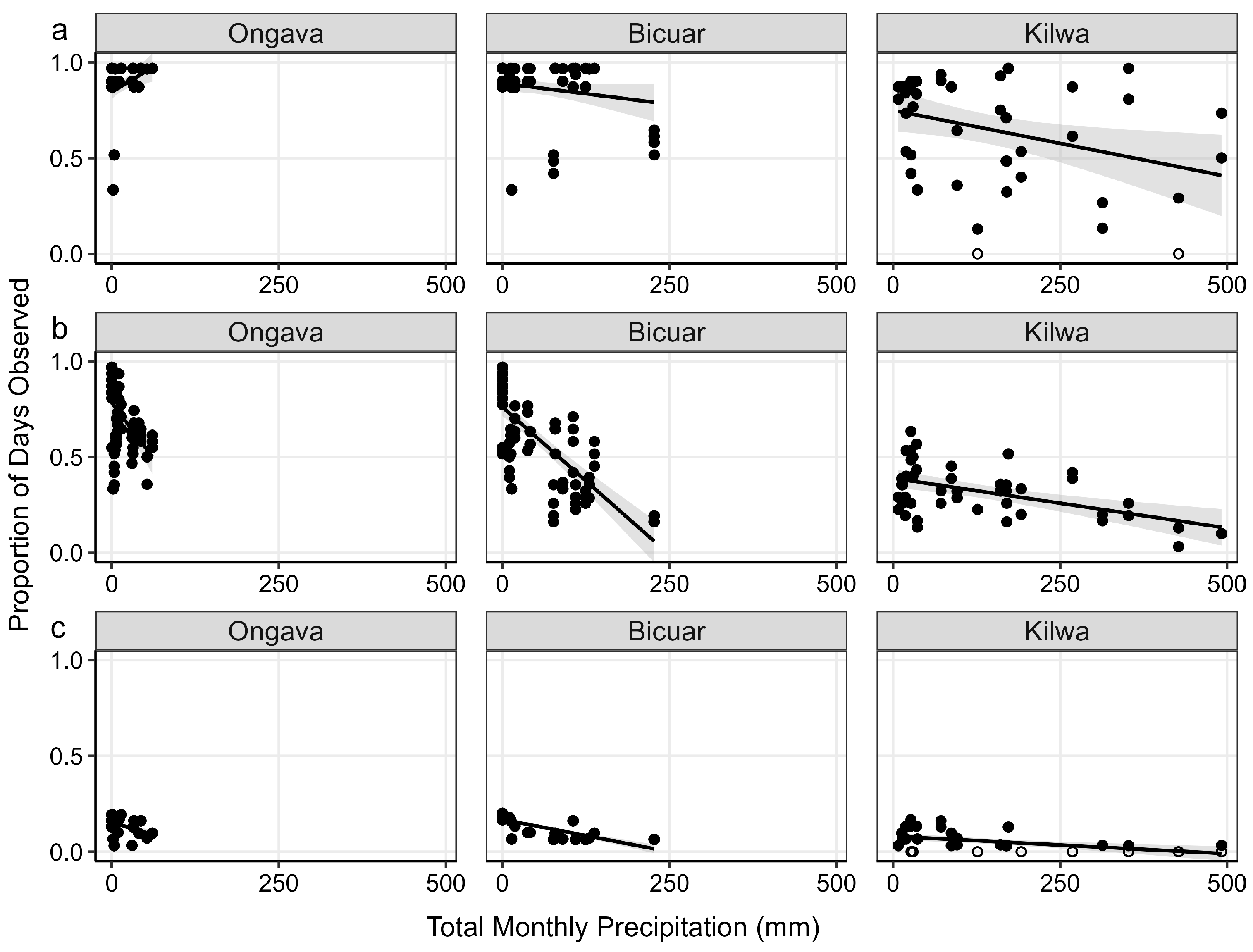

Disclaimer/Publisher’s Note: The statements, opinions and data contained in all publications are solely those of the individual author(s) and contributor(s) and not of MDPI and/or the editor(s). MDPI and/or the editor(s) disclaim responsibility for any injury to people or property resulting from any ideas, methods, instructions or products referred to in the content. |
© 2026 by the authors. Licensee MDPI, Basel, Switzerland. This article is an open access article distributed under the terms and conditions of the Creative Commons Attribution (CC BY) license.