Process-Inspired Latent Dynamics for Direct Multi-Step Regional Sea Surface Temperature Forecasting

Highlights

What are the main findings?

• ADR-Net achieved the lowest aggregate MSE, MAE, and RMSE in all 36 evaluated region–horizon–metric comparisons.
• The process-inspired ADR stream and TPM provided complementary gains in the ECS seven-day ablation study, with larger TPM effects at later lead days.

What is the implication of the main finding?

• Combining structured latent operators with direct temporal projection improved SST-only regional forecasting without autoregressive feedback.

Abstract

Sea surface temperature (SST) forecasts support marine environmental monitoring, hazard assessment, and operational ocean services. Regional multi-step prediction remains difficult because SST-only models must represent transport, spatial spreading, and local nonlinear variation from historical fields while avoiding the recursive use of predicted states. We propose ADR-Net, a direct multi-step forecasting model that combines a flexible data-driven stream with a process-inspired advection–diffusion–reaction (ADR) stream in a shared latent bottleneck. The ADR stream organizes latent SST evolution through three operators that represent transport-like displacement, spatial spreading, and local nonlinear variation. A temporal projection module (TPM) then projects the fused latent representation and multi-scale encoder features directly to all forecast leads. We evaluated ADR-Net against eight learned baselines and two non-learned references using daily OISST v2.1 data from the East China Sea (ECS), South China Sea (SCS), Niño 1+2, and Niño 3.4 regions. Separate models were trained with output lengths $L\in \{1,7,13\}$. ADR-Net achieved the lowest MSE, MAE, and RMSE in all 12 region–output length settings across four regions and three output lengths. In the ECS, it reduced the MSE by 1.46%, 8.07%, and 5.70% relative to the best MSE baseline for $L=1$, $L=7$, and $L=13$, respectively. For the ECS $L=13$ task, ADR-Net maintained the lowest MAE and highest SSIM at every lead day and extended the mean effective forecast horizon from 3.91 to 4.49 days under grid cell thresholds of RMSE ≤ 0.7 °C and $R^2\ge 0.95$. Component ablations on the ECS seven-day task showed that removing the TPM or the process-inspired ADR stream increased the mean MSE by 4.55% and 3.86%, respectively, while removing both increased it by 8.32%. ADR-Net used 7.09 million parameters and 13.07 GFLOPs per ECS seven-day forecast sample. Across four storm-associated episodes, ADR-Net achieved the lowest event-mean cooling footprint MAE at every forecast lead from day 1 to day 13. Together, these results support the combination of process-inspired latent modeling and direct temporal projection for accurate, spatially coherent regional SST forecasting.

1. Introduction

The sea surface temperature (SST) characterizes upper-ocean thermal conditions and is a fundamental variable for monitoring air–sea exchanges, weather and climate, marine ecosystems, and operational ocean applications [1,2]. The SST is also closely coupled to tropical cyclone development and the oceanic cold wakes generated by strong storm forcing [3]. Accurate regional SST forecasts can therefore support ocean monitoring, fishery management, offshore operations, and hazard warnings. Forecasting remains difficult because ocean currents, mixing between surface and deeper waters, heat exchange at the sea surface, and changing weather conditions all affect the SST. In coastal waters and seas along continental margins, complex coastlines, boundaries between warm and cold water, and storms can rapidly alter temperature patterns, making accurate forecasting particularly challenging.

Existing SST forecasting methods mainly fall into numerical and data-driven categories [4]. Numerical models use physical equations together with environmental information, such as wind and heat exchange, to calculate future ocean conditions. Their predictions, however, depend on the quality of the initial data, the treatment of regional boundaries, and model simplifications. Producing forecasts with finer spatial detail also requires considerably more computation. Data-driven models instead learn patterns from historical SST records. Recurrent and convolutional architectures have been used to forecast regional SST fields [5,6,7,8]; graph-based models capture correlations across locations and regions [9,10]; and unified or knowledge-enhanced models incorporate multiple ocean factors, temporal scales, or domain knowledge [11,12]. Geographical and temporal variations in SST predictability, together with increasing errors at longer lead times [13], motivate representations that capture regional SST evolution throughout a multi-step forecast.

Physics-guided machine learning seeks to incorporate scientific knowledge into data-driven models [14,15]. Previous forecasting studies have encoded advection-based state evolution or separated physical dynamics from residual factors in the latent space [16,17]. For SST prediction, physical or numerical variables, partial differential equation constraints, mixed-layer heat budget information, and auxiliary ocean current features have been used to guide deep networks [18,19,20,21]. For regional forecasting from an SST history, the central design problem is to connect representations of SST evolution with the generation of future fields across multiple leads. Process-inspired latent operators can organize transport-like displacement, spatial spreading, and local nonlinear variation, while direct multi-step prediction maps the observed history to the forecast sequence [22]. Integrating these functions within a shared representation provides a framework for coupling structured latent changes with lead-specific prediction.

To address these challenges, we propose ADR-Net, a network inspired by advection–diffusion–reaction (ADR) processes, for direct multi-step SST forecasting. ADR-Net comprises a dual-stream latent bottleneck and a temporal projection module (TPM). The bottleneck contains two complementary streams. The data-driven stream learns flexible spatiotemporal patterns, whereas the process-inspired ADR stream represents latent changes through separate advection-like, diffusion-like, and reaction-like operators. After the two streams are fused, the TPM projects the latent history onto all lead days in parallel, conditioned on the observed sequence. It also transfers spatial information retained by the encoder to the corresponding future states. The decoder then predicts temperature changes relative to the latest observation and generates the complete forecast sequence in a single forward pass.

The main contributions of this study are as follows:

• We develop a dual-stream latent bottleneck that integrates flexible data-driven representation learning with process-inspired ADR modeling. Separate advection-like, diffusion-like, and reaction-like operators structure latent SST changes, and a learnable channelwise gate combines the two streams for forecasting.
• We introduce the TPM for direct multi-step forecasting. The TPM maps historical latent states and multi-scale encoder features to each forecast lead, conditioned on the observed sequence, enabling ADR-Net to generate all future SST fields without autoregressive feedback.
• We demonstrate consistent aggregate accuracy gains across four OISST v2.1 regions and three output lengths of 1, 7, and 13 days. Detailed ECS evaluations establish leadwise accuracy and spatial structure preservation, quantify the component contributions and computational cost, and assess forecasts against in situ observations and across four storm-associated episodes.

2. Materials and Methods

2.1. Data

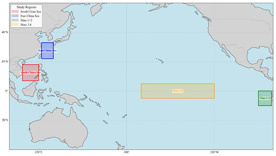
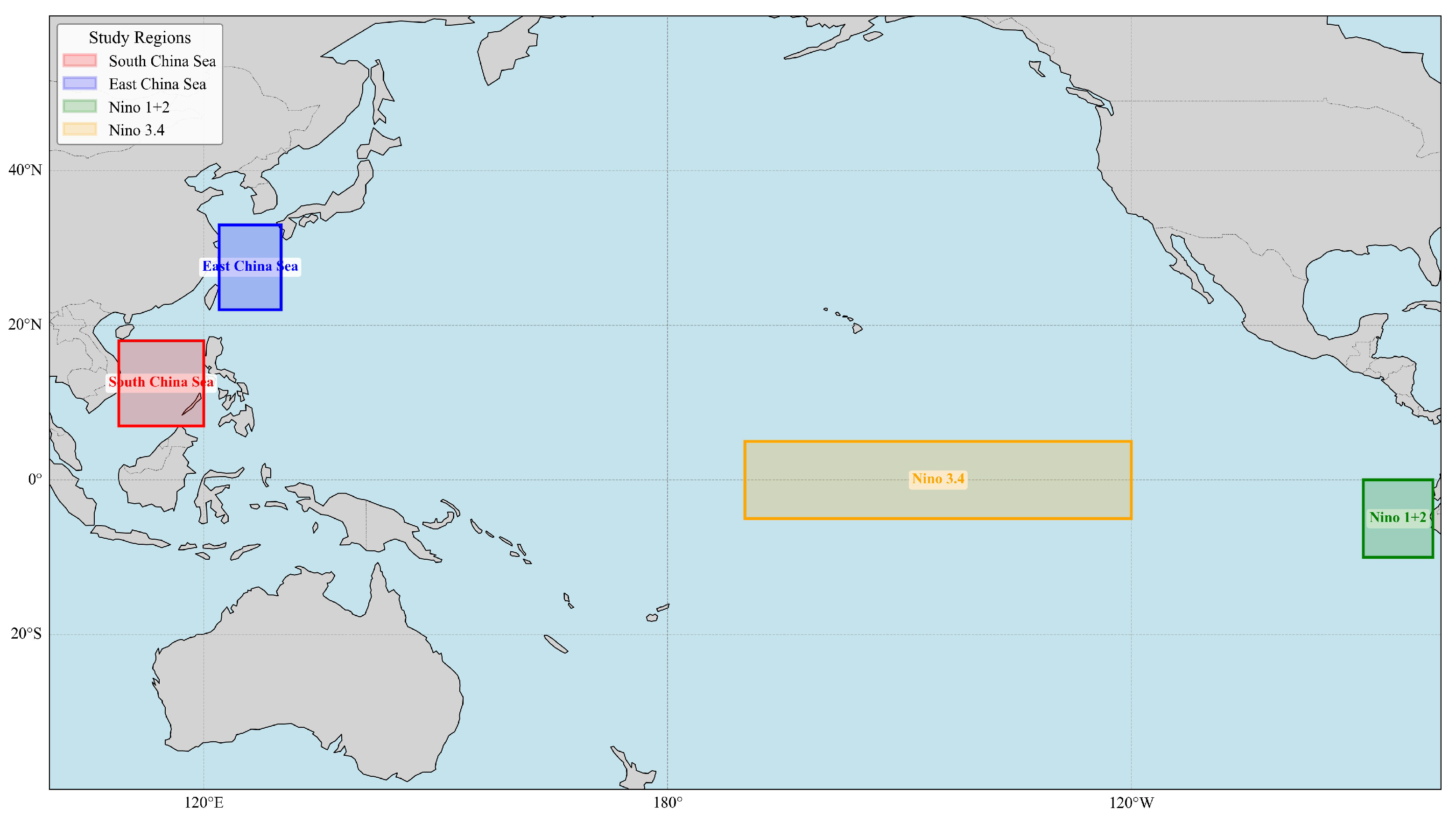
This study uses Version 2.1 of the Optimum Interpolation Sea Surface Temperature dataset (OISST v2.1) released by the National Oceanic and Atmospheric Administration (NOAA). The dataset is publicly available from the NOAA National Centers for Environmental Information (https://doi.org/10.25921/RE9P-PT57). It blends satellite and in situ observations to provide daily global SST fields at a spatial resolution of 0.25° × 0.25° [23]. We evaluated the models in four regions: the East China Sea (ECS), the South China Sea (SCS), Niño 1+2, and Niño 3.4. Table 1 and Figure 1 show their geographical boundaries, grid sizes, and locations. These regions cover rapidly changing marginal seas and more slowly varying equatorial Pacific waters, representing distinct regional settings for the evaluation of forecast accuracy.

Table 1. Geographical ranges and grid sizes of the four OISST v2.1 study regions.

Region	Latitude	Longitude	Grid Size
East China Sea (ECS)	22.125°N–32.875°N	122.125°E–129.875°E	$44\times 32$
South China Sea (SCS)	8.125°N–17.875°N	110.125°E–119.875°E	$40\times 40$
Niño 1+2	9.875°S–0.125°S	270.125°E–277.875°E	$40\times 32$
Niño 3.4	4.875°S–4.875°N	190.125°E–239.875°E	$40\times 200$

Figure 1. Locations and geographical extents of the four OISST v2.1 study regions.

We selected the ECS for detailed analyses because its rapidly varying marginal-sea SST and the Typhoon In-fa cooling event provide a common setting for examining forecast accuracy and event-scale evolution. Using this domain throughout the detailed evaluation connects leadwise errors, spatial forecast patterns, storm-associated SST changes, and component contributions within a consistent regional framework.

For all four regions, the data spanned 1 January 1982 to 31 December 2022. We divided each regional dataset chronologically, using 1982–2010 for training, 2011–2016 for validation, and 2017–2022 for testing.

For an external point observation evaluation of the ECS $L=13$ forecasts, we additionally used NOAA iQuam V2.10 in situ SST observations [24] from the 2017–2022 test period. We retained observations with the highest iQuam quality level (quality level 5) inside the ECS domain. Repeated measurements were averaged by UTC date, platform identifier, and platform type, together with their observation positions. For each forecast lead, the gridded prediction was bilinearly interpolated to the corresponding platform-day mean position. We report the MAE, RMSE, and bias, where bias is the prediction minus iQuam. OISST is included as an analysis reference to contextualize differences between gridded SST and point observations; forecast model rankings are calculated among the learned models.

2.2. Data Preprocessing and Sample Construction

To construct complete rectangular SST fields, missing grid cell values, including land-associated missing cells within the regional domains, were filled independently in each daily field using spatial bilinear interpolation based on available neighboring SST values. The interpolated fields were subsequently normalized and supplied to the forecasting models. The same preprocessing procedure was applied consistently to all four study regions.

Within each temporal split, consecutive SST fields were converted into input–target samples using a sliding window with a stride of $1\mathrm{d}$. Taking day t as the final day of the input sequence, the model uses $T=12$ consecutive daily SST fields ending on day t to construct targets over the subsequent $L\mathrm{d}$, where $L\in \{1,7,13\}$:

$${\mathcal{X}}_t=[{\mathbf{S}}_{t-T+1},\dots ,{\mathbf{S}}_t],{\mathcal{Y}}_t^{\left(L\right)}=[{\mathbf{S}}_{t+1},\dots ,{\mathbf{S}}_{t+L}].$$

The same sample construction procedure was applied to all output lengths. For ADR-Net and each learned baseline, a separate model was trained for each $L\in \{1,7,13\}$. Each model was evaluated on its complete target sequence, from day $t+1$ to day $t+L$. Taking $L=7$ as an example, the ECS training, validation, and test sets contained 10,574, 2174, and 2173 samples, respectively, with input and target tensor shapes of $N\times 12\times 1\times 44\times 32$ and $N\times 7\times 1\times 44\times 32$, respectively. The SST fields were standardized using the global mean and standard deviation of the training period:

$$\tilde{\mathbf{S}}={\displaystyle \frac{\mathbf{S}-{\mu }_{\mathrm{tr}}}{{\sigma }_{\mathrm{tr}}}},$$

where ${\mu }_{\mathrm{tr}}=$ 23.4822 °C and ${\sigma }_{\mathrm{tr}}=$ 4.6309 °C for the ECS dataset. The same statistics were applied to the validation and test sets, and the predictions were transformed back to the original Celsius scale before evaluation.

2.3. Methods

2.3.1. ADR-Net Overview

ADR-Net follows an encoder–bottleneck–decoder architecture that directly maps a historical SST sequence of T time steps to a forecast sequence of L time steps. Here, T and L denote the numbers of input and output time steps, respectively. The input sequence is first processed by a spatiotemporal encoder that extracts multi-scale spatial features while preserving the temporal resolution. The architecture centers on two modules: a dual-stream latent bottleneck for latent dynamics modeling and the TPM for observation-to-forecast temporal mapping.

Within the dual-stream latent bottleneck, the data-driven stream learns flexible spatiotemporal patterns through residual transformations. The process-inspired ADR stream organizes latent SST changes through advection-like, diffusion-like, and reaction-like operators that encode transport, spatial spreading, and local nonlinear variation. A learnable channelwise gate combines the data-driven representation with the fused ADR response, forming a shared representation for direct multi-step prediction.

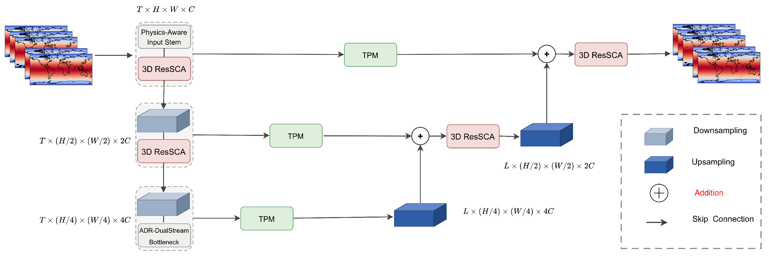
The TPM subsequently maps the shared latent representation to all forecast leads. Conditioned on the input history, it computes adaptive temporal weights that determine each historical state’s contribution to the representation at each forecast lead. These weights generate the complete future latent sequence in parallel, without autoregressive feedback. Scale-specific TPMs also project historical skip features onto the future temporal axis so that they are aligned with the decoder states before fusion. Finally, the decoder progressively restores the spatial resolution and predicts residuals relative to the latest observed SST field, producing the complete multi-step forecast sequence.

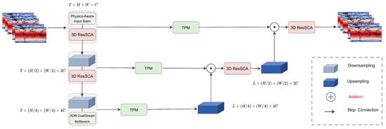
Figure 2 summarizes the overall architecture and the information flow between the dual-stream latent bottleneck, the TPMs, and the multi-scale decoder.

Figure 2. Overall architecture of ADR-Net. The encoder extracts multi-scale spatiotemporal features, the dual-stream latent bottleneck forms the deepest latent representation, and the TPMs project encoder histories to the forecast timeline for future-aligned decoding.

2.3.2. Spatiotemporal Encoder

Figure 2 illustrates the spatiotemporal encoder. Its input is a historical SST sequence $\mathbf{X}\in {\mathbb{R}}^{T\times H\times W\times C_{\mathrm{in}}}$, where T is the number of input days, H and W are the spatial dimensions, and $C_{\mathrm{in}}$ is the number of observed variables at each time step. In this study, $T=12$ and $C_{\mathrm{in}}=1$, with the SST as the sole observed input variable. The fixed-operator input stem derives horizontal Sobel, vertical Sobel, and Laplacian responses from each SST field. These internally derived responses are concatenated with the original SST input and projected into a C-channel latent representation.

The encoder subsequently employs three stages built from three-dimensional residual spatial-and-channel attention (ResSCA) blocks. Each ResSCA block uses two $3\times 3\times 3$ convolutions with group normalization and exponential linear unit (ELU) activation to capture spatiotemporal dependencies. A residual shortcut preserves the input signal, while parallel channel and spatial squeeze-and-excitation branches recalibrate the residual features along the channel and spatial dimensions. Between adjacent stages, a fixed depthwise $1\times 3\times 3$ averaging filter precedes stride-$(1,2,2)$ spatial downsampling, halving the spatial resolution at each scale transition while preserving the historical length T. The subsequent 3D ResSCA stages expand the channel dimensions from C to $2C$ and $4C$, respectively. The first two feature levels are retained as multi-scale histories for TPM-based future alignment, whereas the deepest representation is passed to the dual-stream latent bottleneck.

2.3.3. Dual-Stream Latent Bottleneck

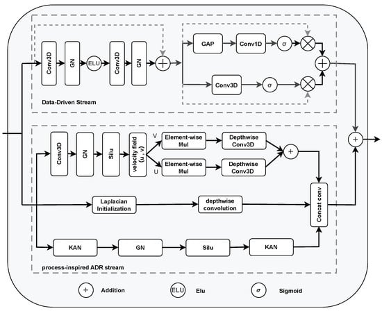
The dual-stream bottleneck combines flexible data-driven representation learning with the process-inspired modeling of latent SST evolution. As illustrated in Figure 3, the deepest encoder feature is fed to the two streams in parallel. The data-driven stream employs a 3D residual block with group normalization, ELU activation, and channel–spatial recalibration to produce the representation ${\mathbf{F}}_{\mathrm{data}}$.

Figure 3. Architecture of the dual-stream latent bottleneck. The data-driven stream extracts flexible spatiotemporal representations, while the process-inspired ADR stream represents advection-, diffusion-, and reaction-like responses in the latent space.

The ADR stream first projects the bottleneck features through a $1\times 1\times 1$ convolution. Differences between consecutive projected historical frames are then added through a learnable scalar coefficient, with the final difference frame set to zero. The resulting temporally augmented representation, denoted by $\mathbf{Z}$, provides the three parallel ADR branches with both spatial features and information about changes between historical states. In the advection branch, an intermediate feature for velocity estimation is extracted using a 3D convolution, group normalization, and sigmoid linear unit (SiLU) activation:

$${\mathbf{H}}_v=\mathrm{SiLU}\left[\mathrm{GN}\left({\mathrm{Conv}}_{3\times 3\times 3}\left(\mathbf{Z}\right)\right)\right].$$

(1)

A $1\times 3\times 3$ convolution then predicts two latent transport components along the x- and y-directions of the spatial grid. Their magnitudes are controlled by a learnable scale and the hyperbolic tangent function:

$$[\widehat{u},\widehat{v}]={\mathrm{Conv}}_{1\times 3\times 3}\left({\mathbf{H}}_v\right),u={\gamma }_v\tanh \left(\widehat{u}\right),v={\gamma }_v\tanh \left(\widehat{v}\right).$$

(2)

The components u and v parameterize directional transport in the latent space. Elementwise multiplication with $\mathbf{Z}$ forms the corresponding latent fluxes, whose negative divergence is evaluated using fixed central-difference operators:

$$\mathcal{A}\left(\mathbf{Z}\right)=-\left[D_x(u\odot \mathbf{Z})+D_y(v\odot \mathbf{Z})\right],$$

(3)

where $D_x$ and $D_y$ denote the central-difference operators along the two spatial directions.

The diffusion branch employs a learnable depthwise spatial convolution initialized with a discrete Laplacian kernel:

$$\mathcal{D}\left(\mathbf{Z}\right)={\tilde{\mathbf{K}}}_d{\ast }_{\mathrm{dw}}\mathbf{Z},{\mathbf{K}}_d^{\left(0\right)}=\left[\begin{array}{ccc}0& 1& 0\\ 1& -4& 1\\ 0& 1& 0\end{array}\right],$$

(4)

where ${\tilde{\mathbf{K}}}_d$ is obtained by subtracting the spatial mean of each depthwise kernel during forward propagation. For each latent frame, the reaction branch uses two Chebyshev-based Kolmogorov–Arnold network (KAN) layers with degree-three polynomial expansions to model local nonlinear variations:

$$\mathcal{R}\left({\mathbf{Z}}_t\right)=e^{s_r}{\mathrm{KAN}}_2\left(\mathrm{SiLU}\left[\mathrm{GN}\left({\mathrm{KAN}}_1\left({\mathbf{Z}}_t\right)\right)\right]\right),$$

(5)

where $e^{s_r}$ is a learnable positive scaling factor.

The three responses are concatenated and fused using a $1\times 1\times 1$ convolution, batch normalization, and SiLU activation. A residual connection is then applied to obtain

$${\mathbf{F}}_{\mathrm{ADR}}=\psi \left(\mathcal{A}\left(\mathbf{Z}\right)\parallel \mathcal{D}\left(\mathbf{Z}\right)\parallel \mathcal{R}\left(\mathbf{Z}\right)\right)+\beta \mathbf{Z},$$

(6)

where $\psi (·)$ denotes the fusion operation and $\beta$ is a learnable residual coefficient. Finally, the data-driven and normalized ADR features are combined using a learnable channelwise convex gate:

$$\mathbf{g}=\sigma \left(\mathbf{a}\right),\mathbf{M}=\mathbf{g}\odot {\mathbf{F}}_{\mathrm{data}}+(1-\mathbf{g})\odot \mathrm{GN}\left({\mathbf{F}}_{\mathrm{ADR}}\right),$$

(7)

where $\mathbf{a}$ contains learnable channelwise gate logits and $\mathbf{g}$ is broadcast over the temporal and spatial dimensions. The gate logits are initialized to 2, giving an initially data-dominant fusion. The resulting shared latent representation $\mathbf{M}$ is subsequently passed to the TPM.

2.3.4. TPM

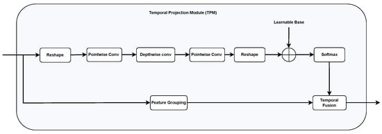
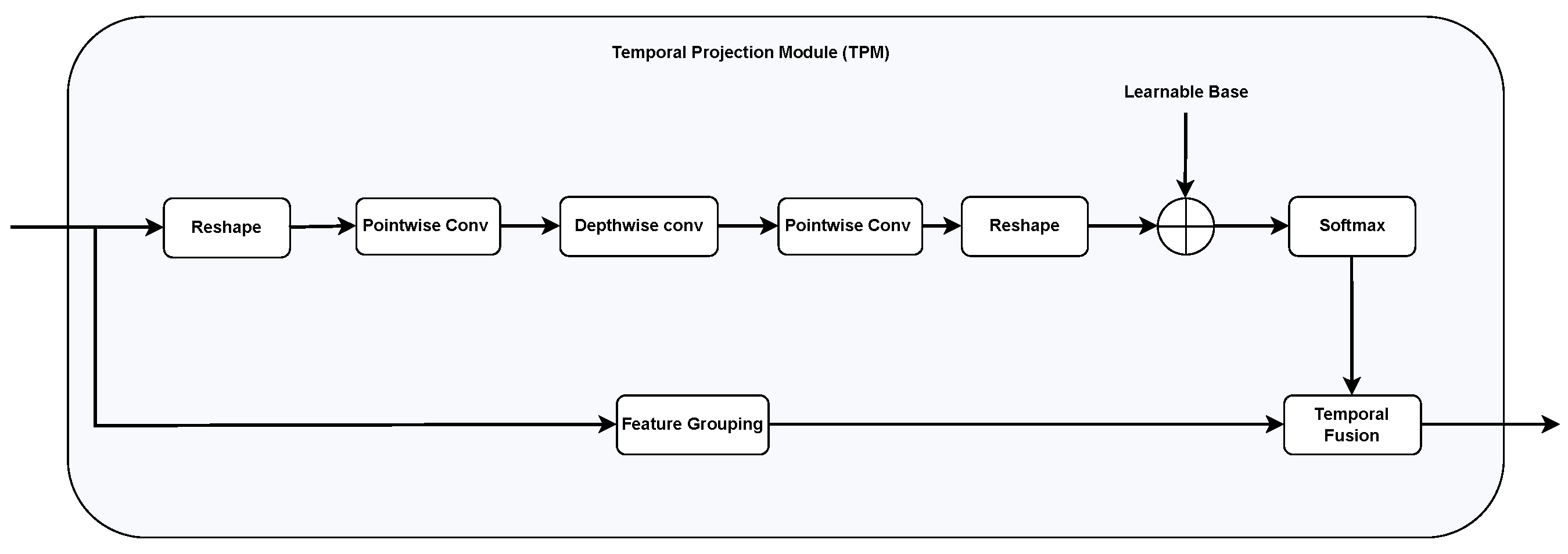
The TPM maps the historical feature sequence to all forecast leads in a single operation. As illustrated in Figure 4, the upper path concatenates the historical frames along the channel dimension and applies pointwise–depthwise–pointwise convolutions to generate an input-adaptive temporal correction. This correction is combined with a learnable groupwise base matrix, and softmax normalization produces the temporal projection weights. The lower path groups the historical features along the channel dimension and uses these weights to aggregate the features over the historical time axis, generating representations for all forecast leads in parallel.

Figure 4. Architecture of the TPM. The groupwise base matrix describes the global correspondence between the observed and forecast timelines, while the convolutional path extracts an adaptive temporal correction from the input history. After softmax normalization, the temporal projection weights aggregate the historical features into all forecast leads in parallel.

At a given feature scale, the TPM receives a mini-batch of historical features $\mathbf{M}\in {\mathbb{R}}^{B\times C\times T\times H\times W}$. Here, B is the batch size, T is the historical sequence length, and C, H, and W denote the channel count and spatial dimensions at this scale. The TPM partitions the channels into G groups and maps the T historical states to L forecast leads in parallel.

A learnable base matrix ${\mathbf{W}}^{\mathrm{base}}\in {\mathbb{R}}^{G\times L\times T}$ provides group-specific temporal projection scores that are shared across samples and spatial locations.

To make this projection input-adaptive, the observed frames are first concatenated along the channel dimension to form a $CT$-channel spatial map. This map is processed by a lightweight pointwise–depthwise–pointwise convolutional path, which predicts an adaptive correction $\Delta \mathbf{W}$ for each sample, channel group, forecast lead, input time, and spatial location. The final temporal projection weights are computed as

$$\mathbf{P}={\mathrm{softmax}}_T\left({\displaystyle \frac{{\mathbf{W}}^{\mathrm{base}}}{\tau }}+\lambda \tanh (\Delta \mathbf{W})\right),$$

(8)

where the base matrix is broadcast over the batch and spatial dimensions. The learnable temperature $\tau$ controls the sharpness of the temporal distribution, and $\lambda$ controls the contribution of the adaptive correction. The softmax is applied over the input-time dimension so that the weights assigned to the observed states sum to one.

The resulting weights are then used to perform a groupwise weighted sum over the observed latent features, producing $\widehat{\mathbf{M}}\in {\mathbb{R}}^{B\times C\times L\times H\times W}$. Thus, the TPM forms a future-aligned latent sequence for all forecast leads without autoregressive feedback. In ADR-Net, the deepest TPM projects the shared latent representation onto the forecast timeline, while scale-specific TPMs apply the same projection principle to align encoder skip features with future decoder states.

2.3.5. Spatial Decoder and Residual Prediction

The spatial decoder progressively restores the forecast features to the input grid resolution while preserving the forecast sequence length L. At each scale, the upsampled features are concatenated with the corresponding TPM-aligned encoder features and refined through convolutional fusion and a ResSCA block. A final $1\times 1\times 1$ convolution predicts SST residuals for all forecast leads. These residuals are multiplied by a learnable scalar and added to the latest observed SST field, broadcast across the forecast sequence, to obtain the complete multi-step prediction.

2.4. Experimental Settings and Evaluation Metrics

All experiments were implemented in PyTorch (version 2.7.0+cu126) [25] using the OpenSTL framework (version 1.0.0) [26]. ADR-Net was compared with eight learned baselines: ConvLSTM [27], PredRNN [28], PredRNN-v2 [29], MIM [30], MAU [31], SimVP [32], TAU [33], and Earthformer [34]. For a contextual comparison, we also evaluated persistence and training-period daily climatology; Appendix A, Appendix A.1 defines these two non-learned references. All methods used the same chronological partitions, input–output settings, normalization procedure, and evaluation code. The training configuration is summarized in Table 2. Training used an NVIDIA GeForce RTX 3090 GPU (NVIDIA Corporation, Santa Clara, CA, USA). For each run, the checkpoint with the lowest validation loss was used for testing.

Table 2. Training settings used in the experiments.

Setting	Value
Optimizer	AdamW (${\beta }_1=0.9$, ${\beta }_2=0.95$)
Initial learning rate	$2\times {10}^{-4}$
Learning rate schedule	5-epoch warm-up followed by cosine annealing
Warm-up starting learning rate	$1\times {10}^{-6}$
Minimum learning rate	$1\times {10}^{-6}$
Weight decay	$5\times {10}^{-4}$
Batch size	8
Gradient clipping	${\mathcal{l}}_2$-norm threshold of 0.5
Maximum training epochs	120
Early stopping	Validation loss with patience of 25 epochs
Minimum validation improvement	$1\times {10}^{-4}$
Random seed	2025
Training device	NVIDIA GeForce RTX 3090 GPU

All predictions were transformed back to the original Celsius scale before evaluation. The mean absolute error (MAE), mean squared error (MSE), and root mean squared error (RMSE) were used as the primary metrics. Let $\Omega$ denote all SST values included in a reported forecast setting. These metrics are defined as

$$\mathrm{MAE}={\displaystyle \frac{1}{|\Omega |}}\sum _{i\in \Omega }\left|{\widehat{S}}_i-S_i\right|,$$

(9)

and

$$\begin{array}{cc}\hfill \mathrm{MSE}& ={\displaystyle \frac{1}{|\Omega |}}\sum _{i\in \Omega }{\left({\widehat{S}}_i-S_i\right)}^2,\hfill \\ \hfill \mathrm{RMSE}& =\sqrt{\mathrm{MSE}}.\hfill \end{array}$$

(10)

Here, ${\widehat{S}}_i$ and $S_i$ denote the predicted SST and the corresponding OISST reference SST, respectively. The MAE and RMSE are expressed in °C, whereas the MSE is expressed in (°C)²; lower values indicate better performance. For the detailed ECS diagnostics, the coefficient of determination ($R^2$) and the structural similarity index (SSIM) [35] were additionally used to assess agreement with the reference SST and the preservation of the spatial structure, respectively.

3. Results

3.1. Accuracy Analysis

3.1.1. Aggregate Accuracy Across Regions and Output Lengths

ADR-Net achieved the lowest MSE, MAE, and RMSE in all 12 region–output length settings across the four OISST v2.1 regions and three output lengths (Table 3). In the ECS, ADR-Net obtained MSE/MAE values of 0.0808/0.1880, 0.3294/0.4058, and 0.4868/0.5040 for $L=1$, $L=7$, and $L=13$, respectively. These MSE values were 1.46%, 8.07%, and 5.70% lower than those of the strongest MSE baseline at the corresponding output lengths.

Table 3. Overall forecasting errors of nine learned models and two non-learned reference baselines across the four study regions and output lengths $L=1$, $L=7$, and $L=13$.

Cls.	Method	$\mathit{L}=1$			$\mathit{L}=7$			$\mathit{L}=13$
		MSE	MAE	RMSE	MSE	MAE	RMSE	MSE	MAE	RMSE
East China Sea (ECS)
B	Persistence	0.0960	0.2025	0.3099	0.4703	0.4822	0.6858	0.8165	0.6476	0.9036
	Climatology	1.2400	0.8872	1.1136	1.2399	0.8871	1.1135	1.2399	0.8870	1.1135
R	ConvLSTM	0.0913	0.2104	0.3022	0.3949	0.4618	0.6284	0.6442	0.6059	0.8026
	PredRNN	0.0820	0.1945	0.2864	0.3695	0.4337	0.6079	0.5636	0.5599	0.7507
	PredRNN-v2	0.0897	0.2058	0.2995	0.3662	0.4383	0.6051	0.5922	0.5693	0.7695
	MIM	0.0853	0.1997	0.2921	0.3718	0.4429	0.6098	0.6059	0.5834	0.7784
	MAU	0.1013	0.2235	0.3183	0.4611	0.5003	0.6790	0.6477	0.6107	0.8048
C	SimVP	0.1017	0.2227	0.3189	0.4169	0.4848	0.6457	0.5162	0.5368	0.7185
	TAU	0.0901	0.2097	0.3002	0.3583	0.4364	0.5986	0.5603	0.5600	0.7486
A	Earthformer	0.1219	0.2499	0.3491	0.3755	0.4496	0.6128	0.5706	0.5710	0.7554
P	ADR-Net	0.0808	0.1880	0.2843	0.3294	0.4058	0.5739	0.4868	0.5040	0.6977
South China Sea (SCS)
B	Persistence	0.0460	0.1448	0.2145	0.1936	0.3177	0.4400	0.3123	0.4094	0.5588
	Climatology	0.7363	0.7043	0.8581	0.7367	0.7044	0.8583	0.7368	0.7044	0.8584
R	ConvLSTM	0.0474	0.1572	0.2177	0.1833	0.3144	0.4281	0.3614	0.4589	0.6012
	PredRNN	0.0416	0.1434	0.2040	0.1934	0.3188	0.4398	0.3109	0.4232	0.5576
	PredRNN-v2	0.0454	0.1527	0.2131	0.1757	0.3106	0.4192	0.2880	0.4012	0.5367
	MIM	0.0435	0.1484	0.2086	0.1723	0.3057	0.4151	0.2795	0.3965	0.5287
	MAU	0.0491	0.1596	0.2216	0.2277	0.3520	0.4772	0.3919	0.4556	0.6260
C	SimVP	0.0474	0.1570	0.2177	0.2124	0.3410	0.4609	0.3157	0.4246	0.5619
	TAU	0.0418	0.1423	0.2045	0.1784	0.3078	0.4224	0.2553	0.3798	0.5053
A	Earthformer	0.0413	0.1430	0.2032	0.1780	0.3157	0.4219	0.2878	0.4078	0.5365
P	ADR-Net	0.0403	0.1378	0.2007	0.1608	0.2927	0.4010	0.2430	0.3650	0.4929
Niño 1+2 Region
B	Persistence	0.0650	0.1614	0.2550	0.4088	0.4194	0.6393	0.7045	0.5754	0.8393
	Climatology	1.2511	0.8818	1.1185	1.2519	0.8819	1.1189	1.2520	0.8819	1.1189
R	ConvLSTM	0.0649	0.1723	0.2548	0.3711	0.4248	0.6092	0.5508	0.5899	0.7422
	PredRNN	0.0523	0.1514	0.2287	0.2934	0.3668	0.5417	0.4784	0.4822	0.6917
	PredRNN-v2	0.0574	0.1605	0.2396	0.3120	0.3796	0.5586	0.4873	0.4882	0.6981
	MIM	0.0571	0.1623	0.2390	0.3165	0.3898	0.5626	0.5134	0.5071	0.7165
	MAU	0.0659	0.1786	0.2567	0.3663	0.4260	0.6052	0.6130	0.5558	0.7829
C	SimVP	0.0719	0.1900	0.2681	0.3208	0.3989	0.5664	0.5012	0.5112	0.7080
	TAU	0.0546	0.1526	0.2337	0.2881	0.3619	0.5367	0.4395	0.4606	0.6629
A	Earthformer	0.0556	0.1576	0.2357	0.3185	0.3965	0.5643	0.4913	0.4954	0.7009
P	ADR-Net	0.0507	0.1461	0.2252	0.2815	0.3497	0.5306	0.4170	0.4391	0.6458
Niño 3.4 Region
B	Persistence	0.0347	0.1300	0.1861	0.2073	0.3069	0.4553	0.3395	0.3982	0.5826
	Climatology	0.7290	0.6972	0.8538	0.7298	0.6976	0.8543	0.7306	0.6979	0.8547
R	ConvLSTM	0.0258	0.1169	0.1606	0.1284	0.2591	0.3583	0.1874	0.3103	0.4329
	PredRNN	0.0230	0.1087	0.1517	0.0967	0.2212	0.3110	0.1747	0.3012	0.4180
	PredRNN-v2	0.0253	0.1152	0.1591	0.1025	0.2318	0.3202	0.1570	0.2842	0.3962
	MIM	0.0246	0.1126	0.1568	0.1215	0.2522	0.3486	0.1693	0.2907	0.4115
	MAU	0.0278	0.1226	0.1667	0.1289	0.2600	0.3590	0.2182	0.3418	0.4671
C	SimVP	0.0264	0.1181	0.1625	0.1114	0.2436	0.3338	0.1566	0.2880	0.3957
	TAU	0.0253	0.1139	0.1591	0.1098	0.2360	0.3314	0.1684	0.2951	0.4104
A	Earthformer	0.0274	0.1211	0.1655	0.1140	0.2457	0.3376	0.1892	0.3184	0.4350
P	ADR-Net	0.0226	0.1069	0.1503	0.0919	0.2161	0.3031	0.1409	0.2681	0.3754

Note: Lower values are better. MSE is reported in (°C)², whereas MAE and RMSE are reported in °C. The best value within each region, output length, and metric is shown in bold, and the second-best value is underlined. Class labels are B = non-learned baseline, R = recurrent, C = convolutional, A = attention-based, and P = proposed.

The aggregate advantage remained consistent in the other three regions. Across $L=1$, $L=7$, and $L=13$, the MSE reductions relative to the strongest baseline ranged from 2.42% to 6.67% in the SCS, from 2.29% to 5.12% in Niño 1+2, and from 1.74% to 10.03% in Niño 3.4. The improvement magnitude varied by region and output length, but ADR-Net reduced the MSE in all 12 region–output length settings.

Paired moving-block bootstrap comparisons supported ADR-Net’s lower test-period errors in the ECS $L=13$ task. The 95% confidence intervals for the MSE, MAE, and RMSE differences between each learned baseline and ADR-Net were all above zero. Appendix A, Appendix A.3 reports the estimates and confidence intervals.

3.1.2. Leadwise Accuracy and Spatial Error Patterns

Across the ECS tasks with $L=1$, 7, and 13, ADR-Net achieved the highest SSIM at every available forecast lead. Appendix A, Appendix A.5 presents the per-lead MSE and SSIM comparisons, extending the aggregate evaluation to accuracy and spatial structure preservation throughout each forecast sequence.

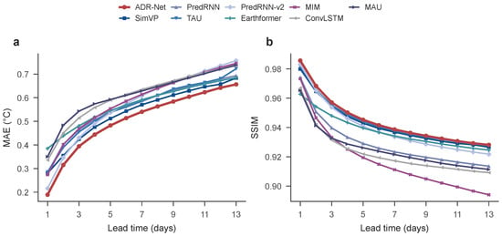
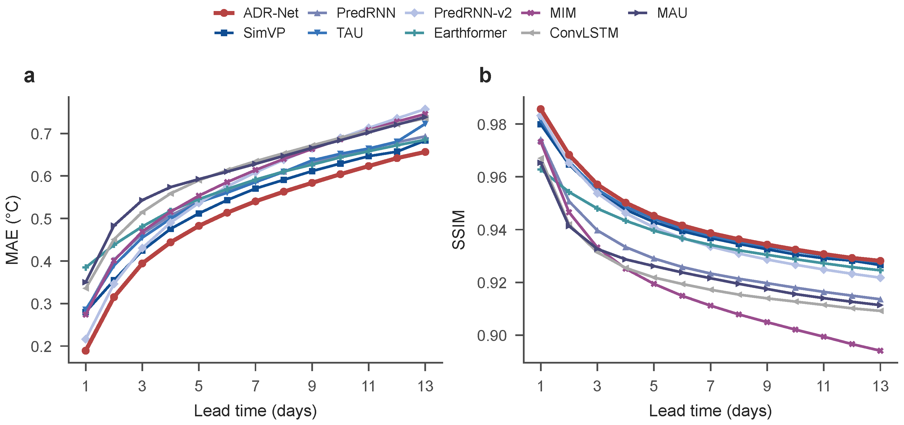
In the independently trained ECS $L=13$ task, ADR-Net maintained the lowest MAE and highest SSIM at every lead day (Figure 5). The MAE increased and the SSIM decreased with the lead time for all models. ADR-Net’s MAE values were 0.1890, 0.5403, and 0.6565 °C at lead days 1, 7, and 13, respectively. These values were 12.59%, 5.28%, and 3.94% lower than the lowest baseline MAE at the corresponding leads. The corresponding SSIM values for ADR-Net were 0.9856, 0.9387, and 0.9281.

Figure 5. Lead time-dependent performance over the 13-day forecast sequence on the ECS test set. (a) Per-lead MAE, for which lower values indicate better performance; (b) per-lead SSIM, for which higher values indicate better spatial structure preservation.

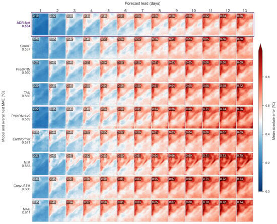
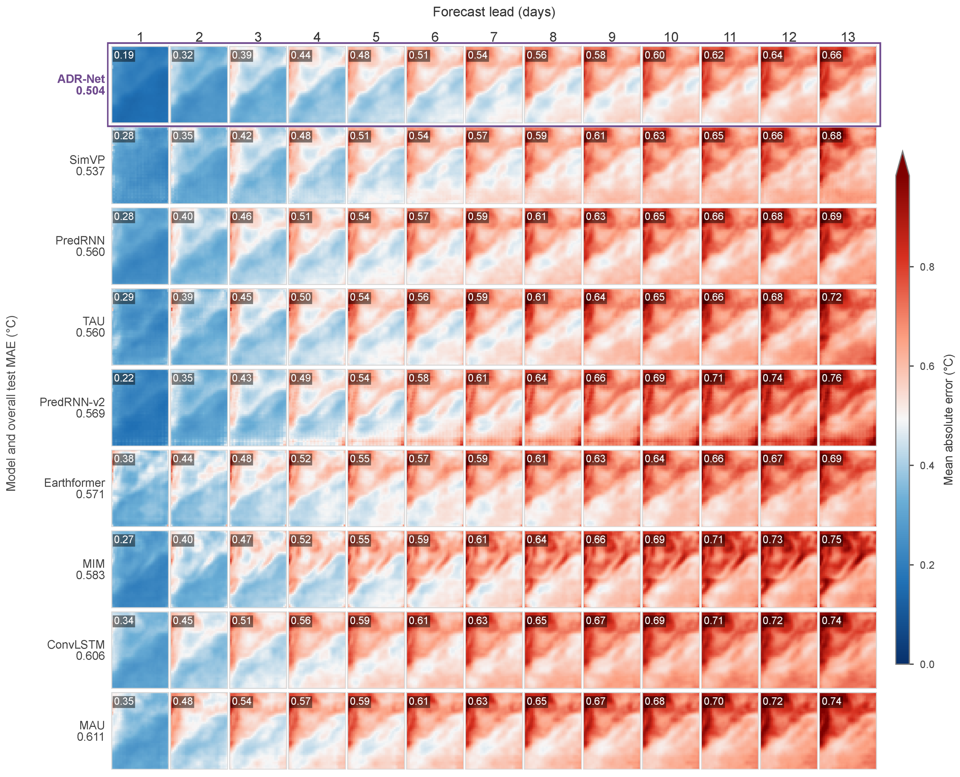
Figure 6 resolves the ECS forecast errors by grid cell and lead day, complementing the domain-averaged curves in Figure 5. Each map reports the grid cell MAE across 2167 test sequences, and the common color scale enables the direct comparison of the error distributions across models and leads. ADR-Net achieved the lowest spatially averaged MAE at all 13 leads, with reductions of 2.32–12.59% relative to the strongest baseline at each lead.

Figure 6. Test-set mean absolute error maps for the 13-day East China Sea (ECS) forecasting task. Each panel shows the grid cell mean of the absolute difference between a model prediction and the Optimum Interpolation Sea Surface Temperature (OISST) reference over 2167 test sequences. Columns denote forecast lead days 1–13, and rows denote independently trained models ordered by their overall test mean absolute error (MAE). All panels share the same linear color scale. The value in each panel is the spatially averaged MAE in degrees Celsius, and the value below each model name is the MAE over all test sequences, grid cells, and forecast leads. ADR-Net is outlined for identification. Model abbreviations are as follows: ADR-Net, advection–diffusion–reaction-inspired network; ConvLSTM, convolutional long short-term memory; PredRNN, predictive recurrent neural network; PredRNN-v2, PredRNN version 2; MIM, memory in memory; MAU, motion-aware unit; SimVP, simple video prediction; TAU, temporal attention unit.

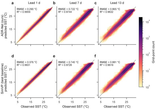
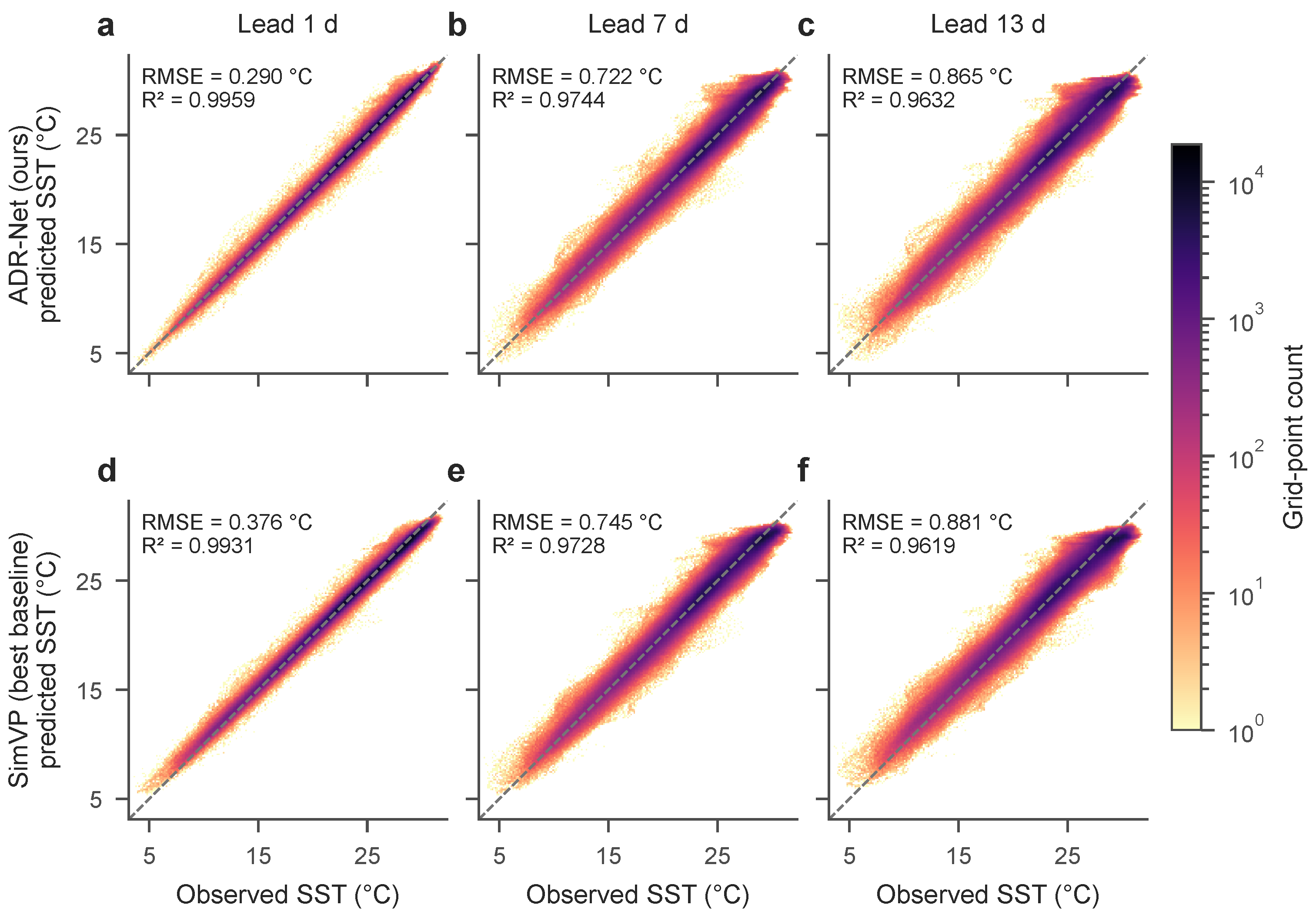
Across all ECS test-set grid points at lead days 1, 7, and 13, ADR-Net showed closer pointwise agreement with the OISST reference than SimVP, the lowest-MAE baseline (Figure 7). For both models, the distributions broadened with the lead time, while the predictions at the cold and warm extremes shifted toward intermediate SST values. These changes were accompanied by higher RMSEs at later leads. At each examined lead, the high-density region for ADR-Net lay visually closer to the 1:1 line than that for SimVP. ADR-Net yielded RMSE values of 0.290, 0.722, and 0.865 °C at lead days 1, 7, and 13, respectively. The corresponding SimVP values were 0.376, 0.745, and 0.881 °C. ADR-Net also achieved $R^2$ values of 0.9959, 0.9744, and 0.9632, compared with 0.9931, 0.9728, and 0.9619 for SimVP.

Figure 7. Density scatter plots of predicted SST against OISST reference SST over all grid points in the ECS test set at lead days 1, 7, and 13. The top and bottom rows show ADR-Net and SimVP, respectively. The dashed line denotes the $1:1$ reference, while darker colors indicate higher grid point counts on a logarithmic scale. RMSE and $R^2$ are reported in each panel.

3.1.3. Effective Forecast Horizon

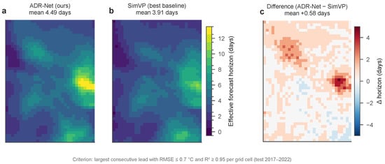
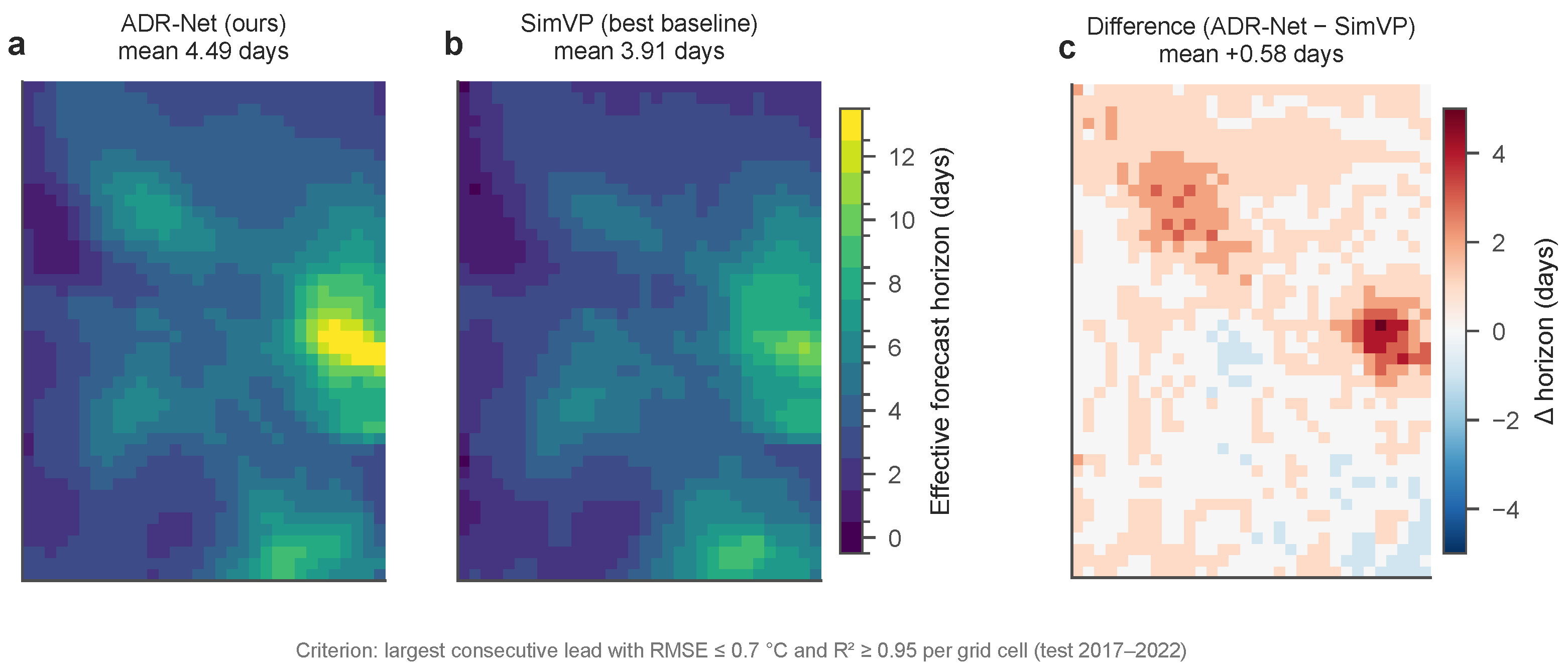
For each grid cell, the effective forecast horizon is defined as the maximum number of consecutive lead days, starting from day 1, for which both RMSE ≤ 0.7 °C and $R^2\ge 0.95$ hold. Under these criteria, ADR-Net increased the mean effective forecast horizon across ECS grid cells from 3.91 days for SimVP to 4.49 days (Figure 8). The proportion of grid cells with an effective forecast horizon of at least seven days increased from 10.6% to 12.3%. The difference map, calculated as ADR-Net minus SimVP, showed longer effective forecast horizons over large parts of the ECS, with shorter horizons confined to fewer grid cells.

Figure 8. Spatial distribution of the effective forecast horizon over the ECS test set. The effective horizon is defined as the maximum number of consecutive lead days from lead day 1 for which the grid cell RMSE is no greater than 0.7 °C and $R^2$ is at least $0.95$: (a) ADR-Net, (b) SimVP, and (c) ADR-Net minus SimVP. Positive differences indicate a longer effective forecast horizon for ADR-Net.

3.2. Storm-Associated SST Evolution

Across four storm-associated episodes, ADR-Net achieved the lowest event-mean cooling footprint MAE in the ECS $L=13$ task: 0.553 °C, compared with 0.621 °C for SimVP, i.e., an 11.0% reduction. This advantage persisted at every forecast lead from day 1 to day 13. ADR-Net also achieved the lowest post-onset MAE over both the cooling footprints and the entire ECS. Appendix A, Appendix A.2 reports the event definitions, regional comparisons, and onset diagnostics. The In-fa case below illustrates the daily cooling–recovery evolution using the $L=1$ forecasts.

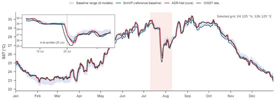
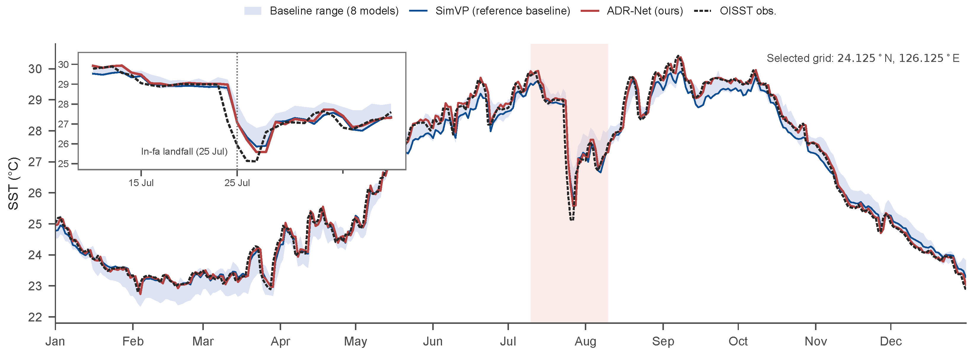
During Typhoon In-fa, the one-day-ahead forecasts from the independently trained ECS $L=1$ models were used to examine SST evolution at the OISST grid cell centered at 24.125°N, 126.125°E. A new one-day-ahead forecast was issued at each daily initialization. The cell was selected objectively as the ECS grid cell with the largest observed SST decrease, 3.03 °C, between the mean fields for 16–19 July and 26–29 July 2021.

The typhoon moved slowly across the ECS in late July 2021 and made landfall near Zhoushan on 25 July [36]. The storm caused ocean mixing and produced a pronounced cold wake within a short period [3,36]. We selected In-fa because its slow translation and pronounced cooling–recovery sequence provide a demanding test of whether an SST-only model can follow event-scale SST evolution. At this grid cell, the lead-day-1 prediction from ADR-Net was compared with the corresponding OISST reference and the lead-day-1 predictions from all eight baseline models (Figure 9). All models shown in this comparison were independently trained for the ECS $L=1$ forecasting task and were evaluated using the same test dates, forecast lead, and grid cell. SimVP was plotted separately as a reference baseline, while the shaded band represents the range spanned by all eight baseline models.

Figure 9. Typhoon In-fa case study at the selected OISST grid cell centered at 4.125°N, 126.125°E. Daily SST in 2021 is shown for the OISST reference and the lead-day-1 predictions from ADR-Net and the eight baseline models independently trained for the ECS $L=1$ forecasting task. SimVP is shown separately as a reference baseline, while the shaded band represents the range spanned by all eight baseline models. The inset enlarges the period affected by Typhoon In-fa, with the landfall date of 25 July marked.

At the selected grid cell, the OISST reference SST fell from 29.9 °C on 12 July to 25.1 °C on 27 July and recovered to 28.1 °C by 15 August (Figure 9). ADR-Net followed the rapid cooling and subsequent recovery more closely than the baseline predictions. Its predicted minimum was 25.6 °C, which was 0.5 °C warmer than the OISST minimum.

The In-fa case illustrates ADR-Net’s ability to track cold wake evolution and subsequent recovery once cooling is represented in the observed SST history (Figure 9). Appendix A, Appendix A.2 evaluates this tracking behavior across four storm-associated episodes using regional, multi-lead comparisons and separately quantifies cooling onset anticipation.

3.3. Evaluation Against In Situ SST

Against quality-5 iQuam observations, ADR-Net achieved the lowest all-platform MAE and RMSE among the nine learned models in the ECS $L=13$ task, with values of 0.7704 and 1.0126 °C, respectively. It ranked first for both metrics at all 13 forecast leads. Paired daily MAE differences between every learned baseline and ADR-Net had 95% confidence intervals above zero. In the two-platform coastal subset, ADR-Net ranked second for both metrics, and the paired MAE difference from TAU had a confidence interval that included zero. Appendix A, Appendix A.4 provides the detailed comparisons.

3.4. Component Analysis

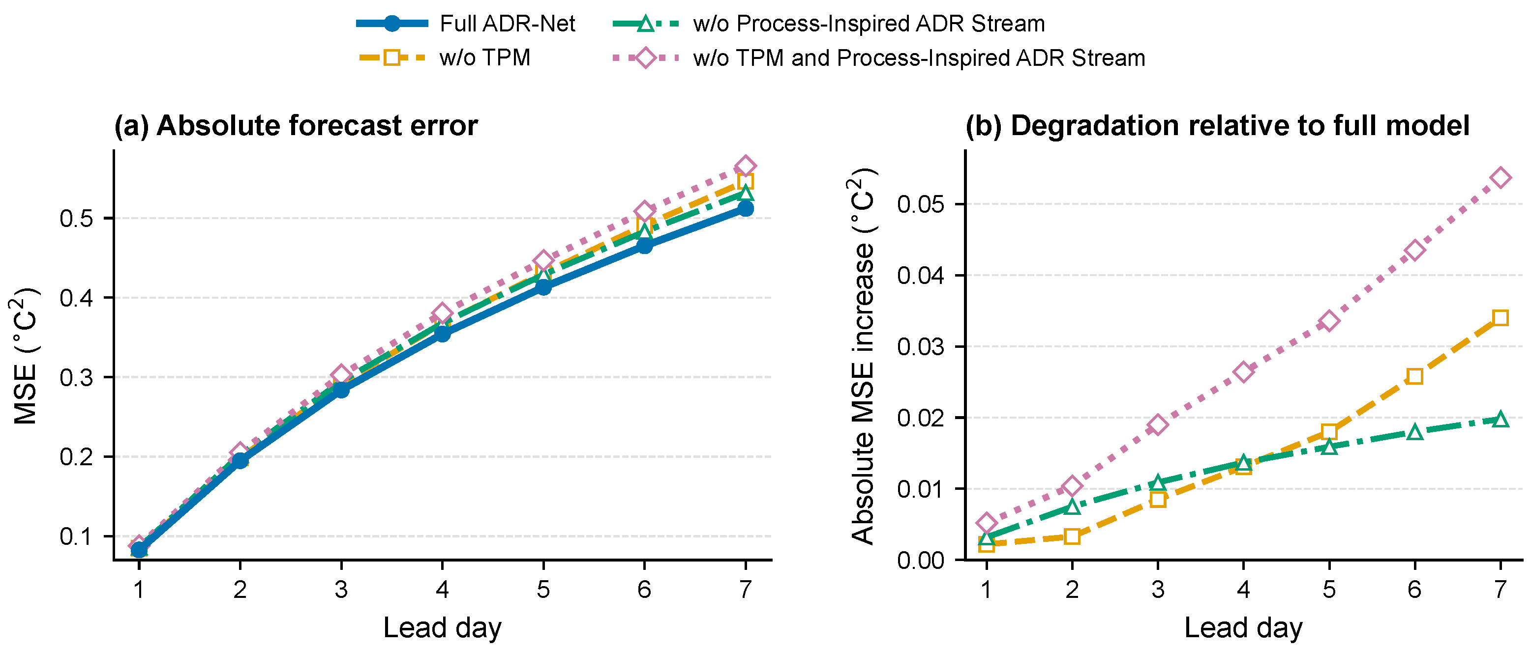
The TPM and the process-inspired ADR stream each contributed to ADR-Net’s seven-day forecasting accuracy on the ECS test set. Three ablated variants were derived from the full ADR-Net by removing the TPM, the process-inspired ADR stream, or both components. Performance was compared using the mean MSE over lead days 1–7, and the results are summarized in Table 4.

Table 4. Component ablation results on the ECS test set for the 7-day forecasting task.

Variant	Mean MSE	Δ vs. Full (%)
Full ADR-Net	0.3294	–
Without TPM	0.3444	+4.55
Without Process-Inspired ADR Stream	0.3421	+3.86
Without TPM and Process-Inspired ADR Stream	0.3568	+8.32

The full ADR-Net achieved the lowest seven-day mean MSE, 0.3294 (°C)² (Table 4). Removing the TPM alone increased the MSE to 0.3444 (+4.55%), and removing the ADR stream alone increased it to 0.3421 (+3.86%). Removing both components increased the MSE to 0.3568 (+8.32%). These comparisons demonstrate that both temporal projection and process-inspired latent modeling contribute to forecast accuracy.

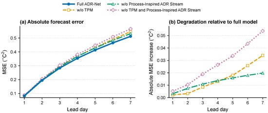
The leadwise ablation results showed that the full ADR-Net retained the lowest MSE throughout the seven-day forecast sequence (Figure 10). Removing the process-inspired ADR stream increased the MSE relative to the full model by 0.0032 (°C)² at lead day 1 and 0.0198 (°C)² at lead day 7. The positive MSE increase at every lead indicated that this stream contributed to lower errors throughout the evaluated sequence.

Figure 10. Leadwise ablation performance on the ECS test set for the 7-day forecasting task. (a) MSE at lead days 1–7 for the full ADR-Net and three ablated variants. (b) Absolute increase in MSE relative to the full model at the same lead day, defined as $\Delta \mathrm{MSE}={\mathrm{MSE}}_{\mathrm{ablated}}-{\mathrm{MSE}}_{\mathrm{full}}$. Lower values indicate better performance. The full model achieves the lowest MSE at every lead day, whereas removing both components results in the largest degradation.

Removing the TPM increased the MSE by 0.0022 (°C)² and 0.0340 (°C)² at lead days 1 and 7, respectively. Its effect exceeded that of removing the process-inspired ADR stream from lead day 5 onward. Within the evaluated ECS $L=7$ task, the TPM therefore had a larger effect at later lead days.

Removing both components produced the largest MSE increase at every lead, reaching 0.0537 (°C)² at lead day 7. At this lead, the joint increase was nearly equal to the sum of the two individual increases (0.0538 (°C)²), consistent with approximately additive ablation effects.

The advection-like, diffusion-like, and reaction-like branches each improved the performance in the ECS $L=7$ comparison. In the branch-level ablations, each latent operator was removed separately, and the resulting degradation was measured relative to the full ADR-Net MSE in the ECS $L=7$ setting.

Removing the advection-like, diffusion-like, and reaction-like branches increased the MSE by 1.54%, 2.94%, and 3.40%, respectively (Table 5), demonstrating the contribution of each operator. The larger increases following the removal of the diffusion-like and reaction-like branches identify these two components as the stronger contributors in the ECS seven-day branch ablation comparison.

Table 5. Branch-level ablation results for the ADR operators on the ECS seven-day forecasting task. Mean MSE is reported in (°C)², and percentage increases are calculated relative to the full ADR-Net.

Variant	Mean MSE	Δ vs. Full (%)
Full	0.3294	–
Without Advection	0.3345	+1.54
Without Diffusion	0.3391	+2.94
Without Reaction	0.3406	+3.40

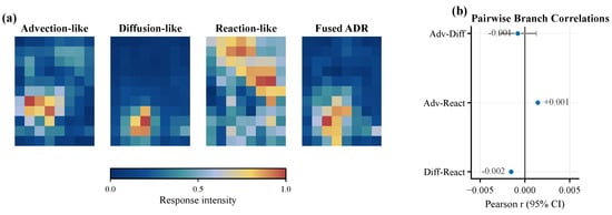
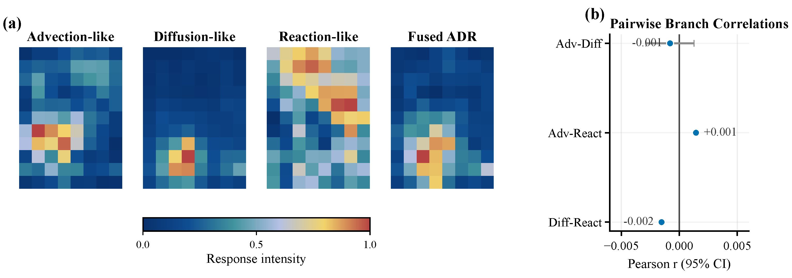
The three ADR branches exhibited differentiated latent response patterns (Figure 11). In the selected ECS test sample, the advection-like, diffusion-like, and reaction-like operators emphasized different spatial responses, which were integrated into the fused ADR representation. Across 2173 test samples, the mean pairwise Pearson correlations were −0.0008 for advection–diffusion, 0.0014 for advection–reaction, and −0.0015 for diffusion–reaction. The distinct response patterns and low mean pairwise correlations, together with the error increases observed in the branch ablations, support the contribution of separate latent operators to the ADR representation.

Figure 11. Spatial response patterns and pairwise correlations of the latent ADR branches. (a) Response intensity maps for the advection-like, diffusion-like, reaction-like, and fused ADR latent responses from the selected ECS test sample. Values are min–max-normalized within each response map for visualization. (b) Pairwise Pearson correlations among latent ADR branch responses over 2173 ECS test samples. Points denote mean correlations and horizontal bars denote 95% confidence intervals.

3.5. Computational Efficiency

We evaluate computational efficiency through model complexity and the measured runtime. For the ECS $L=7$ task, the parameter counts and FLOPs characterize the resources associated with the accuracy results and component ablations. For the ECS $L=13$ task, the measured training and inference times quantify the cost of training each model and generating a complete 13-day forecast.

In the ECS seven-day task, ADR-Net achieved the lowest mean MSE with 7.09 million parameters and 13.07 GFLOPs per forecast sample (Table 6). It ranked second-lowest in terms of the parameter count and fourth-lowest in terms of the computational cost among the nine learned models, combining leading forecast accuracy with fewer parameters and a lower computational cost than all recurrent baselines.

Table 6. Model complexity and computational costs of ADR-Net and the baseline models on the ECS 7-day forecasting task.

Model	Parameters (M)	FLOPs (G)
ConvLSTM	14.93	97.33
PredRNN	23.57	199.00
PredRNN-v2	23.58	200.00
MIM	37.99	310.00
MAU	14.16	28.36
SimVP	12.76	4.82
TAU	12.22	4.60
Earthformer	2.36	5.10
ADR-Net	7.09	13.07

Table 7 compares the training and inference efficiency of the independently trained ECS $L=13$ models. On a single NVIDIA GeForce RTX 3090 GPU with a batch size of 8, ADR-Net completed 32 epochs in 2 h 10 min, averaging 4.1 min per epoch. This training time was shorter than those of all recurrent baselines and comparable to that of Earthformer. ADR-Net generated a complete 13-step forecast in 6.757 ms per sample, substantially faster than the recurrent models. The training time covers both training and validation until early stopping, while the inference time measures the generation of the complete 13-step forecast.

Table 7. Model-specific training and inference times for the ECS $L=13$ experiment.

Model	Epochs Trained	Average Time per Epoch (min)	Total Training Time	Inference Time (ms/Sample)
ConvLSTM	63	6.0	6 h 20 min	10.825
PredRNN	73	11.3	13 h 45 min	17.708
PredRNN-v2	31	13.1	6 h 45 min	18.094
MIM	71	24.8	29 h 17 min	41.834
MAU	69	7.5	8 h 37 min	12.590
SimVP	32	1.7	53 min	1.961
TAU	34	2.6	1 h 28 min	3.288
Earthformer	33	4.2	2 h 18 min	4.219
ADR-Net	32	4.1	2 h 10 min	6.757

4. Discussion

ADR-Net couples process-inspired latent representation learning with direct temporal projection for regional SST forecasting. Previous studies have incorporated prior dynamics, physical–residual decompositions, and physics-guided constraints into forecasting models [16,17,18,19,20,21]. In ADR-Net, the advection-like, diffusion-like, and reaction-like operators organize changes within the historical latent representation, and the TPM maps this representation and multi-scale encoder features to future leads. This design connects the representation of SST evolution to the construction of the complete forecast sequence.

The component ablations support the distinct roles of these two operations. The ADR stream contributes throughout the evaluated seven-day sequence, while the increasing effect of TPM removal at later leads highlights the importance of temporal projection as the forecast extends further from the observed history. The approximately additive ablation effects at day 7 are consistent with contributions from both operations. Branch-level ablations further show that each ADR operator contributes to the shared representation. Together, these results link forecast accuracy to both the organization of historical features and their mapping to future states.

The spatial diagnostics connect these component-level findings to the quality of the predicted fields. The leadwise SSIM evaluates spatial structure preservation, while the grid cell error maps locate forecast errors within the domain. The effective horizon analysis then expresses the local accuracy as the consecutive lead days satisfying the specified RMSE and $R^2$ criteria. The longer effective horizons show how the accuracy gains translate into sustained forecast quality at individual locations.

The all-platform iQuam evaluation extends the assessment from gridded SST fields to matched point observations. The separate coastal mooring analysis adds information about performance at fixed locations. These comparisons involve different spatial sampling and measurement characteristics, including the platform measurement depth and point-to-grid representativeness. OISST’s incorporation of in situ measurements and iQuam’s use of a gridded SST reference in quality control also define the relationship between the two evaluation sources.

The storm-associated analyses identify cooling–recovery tracking as an application of the learned SST representation. The post-onset regional comparisons and the In-fa time series evaluate the evolution of cooling already represented in the observed history, while the onset diagnostic assesses advance detection as a separate forecasting task. Wind, surface heat flux, ocean currents, and mixed-layer depth provide physically relevant inputs for extending the framework’s representation of storm-driven SST changes [3,36].

The computational results place these forecasting gains in the context of the model cost. ADR-Net combines leading accuracy with lower parameter counts and FLOPs than the recurrent baselines in the seven-day task and faster inference in the 13-day task. These comparisons demonstrate the practical value of combining structured latent modeling with parallel forecast generation.

5. Conclusions

This study developed ADR-Net for direct multi-step regional SST forecasting from historical SST fields. The model integrates process-inspired ADR operators and a flexible data-driven stream within a shared latent bottleneck and then uses the TPM to project the fused representation and multi-scale encoder features to all forecast leads. This architecture connects structured latent modeling with parallel forecast generation.

ADR-Net achieved the lowest aggregate MSE, MAE, and RMSE in all 12 evaluated region–output length settings. Component ablations demonstrated the contributions of both ADR modeling and temporal projection, while the ECS diagnostics established gains in spatial structure preservation and the effective forecast horizon. The iQuam and storm-associated evaluations extended the assessment to matched point observations and cooling–recovery evolution. Together, these findings establish the value of coupling process-inspired latent operators with direct temporal projection for accurate and spatially coherent regional SST forecasting.

Appendix A.1. Skill Relative to Persistence and Climatology

We evaluated ADR-Net against two non-learned reference forecasts to assess whether its accuracy gains extend beyond comparisons with learned models. The persistence forecast repeats the latest observed SST field at every forecast lead. The climatology forecast uses the grid cell calendar-day mean calculated exclusively from the 1982–2010 training period. Both references were evaluated on exactly the same 2017–2022 test targets as the corresponding independently trained ADR-Net model.

For a reference forecast r, the MSE skill score is defined as

$${\mathrm{SS}}_r=1-{\displaystyle \frac{{\mathrm{MSE}}_{\mathrm{ADR-Net}}}{{\mathrm{MSE}}_r}},r\in \{\mathrm{persistence},\mathrm{climatology}\}.$$

A positive value indicates that ADR-Net has a lower MSE than the corresponding reference, zero indicates an equal MSE, and a negative value indicates a higher MSE than the reference.

Across the 12 region–output length settings, ADR-Net achieved MSE skill scores of 0.1245–0.5849 relative to persistence and 0.6074–0.9690 relative to climatology (Figure A1). These scores correspond to MSE reductions of 12.45%–58.49% and 60.74%–96.90%, respectively, demonstrating forecasting gains over both reference methods across all evaluated settings.

Figure A1. Aggregate MSE skill scores of ADR-Net relative to persistence (a) and climatology (b) across the four study regions and output lengths $L=1$, 7, and 13. Each score uses the aggregate MSE over all test samples, forecast leads, and grid cells in the corresponding setting. All scores are positive, indicating that ADR-Net has a lower aggregate MSE than both non-learned references in all 12 region–output length settings.

Figure A1. Aggregate MSE skill scores of ADR-Net relative to persistence (a) and climatology (b) across the four study regions and output lengths $L=1$, 7, and 13. Each score uses the aggregate MSE over all test samples, forecast leads, and grid cells in the corresponding setting. All scores are positive, indicating that ADR-Net has a lower aggregate MSE than both non-learned references in all 12 region–output length settings.

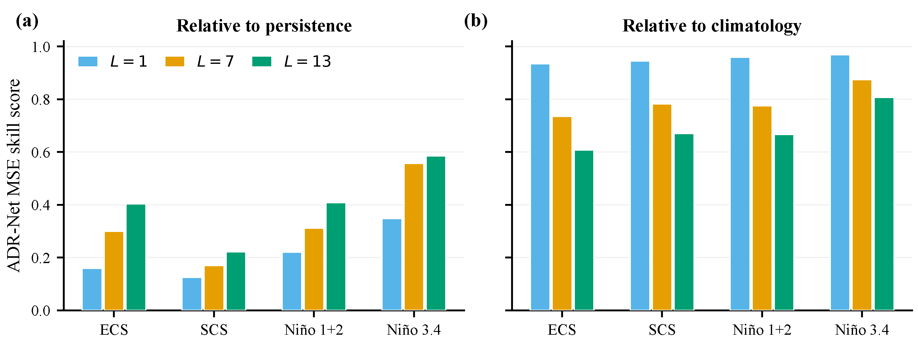
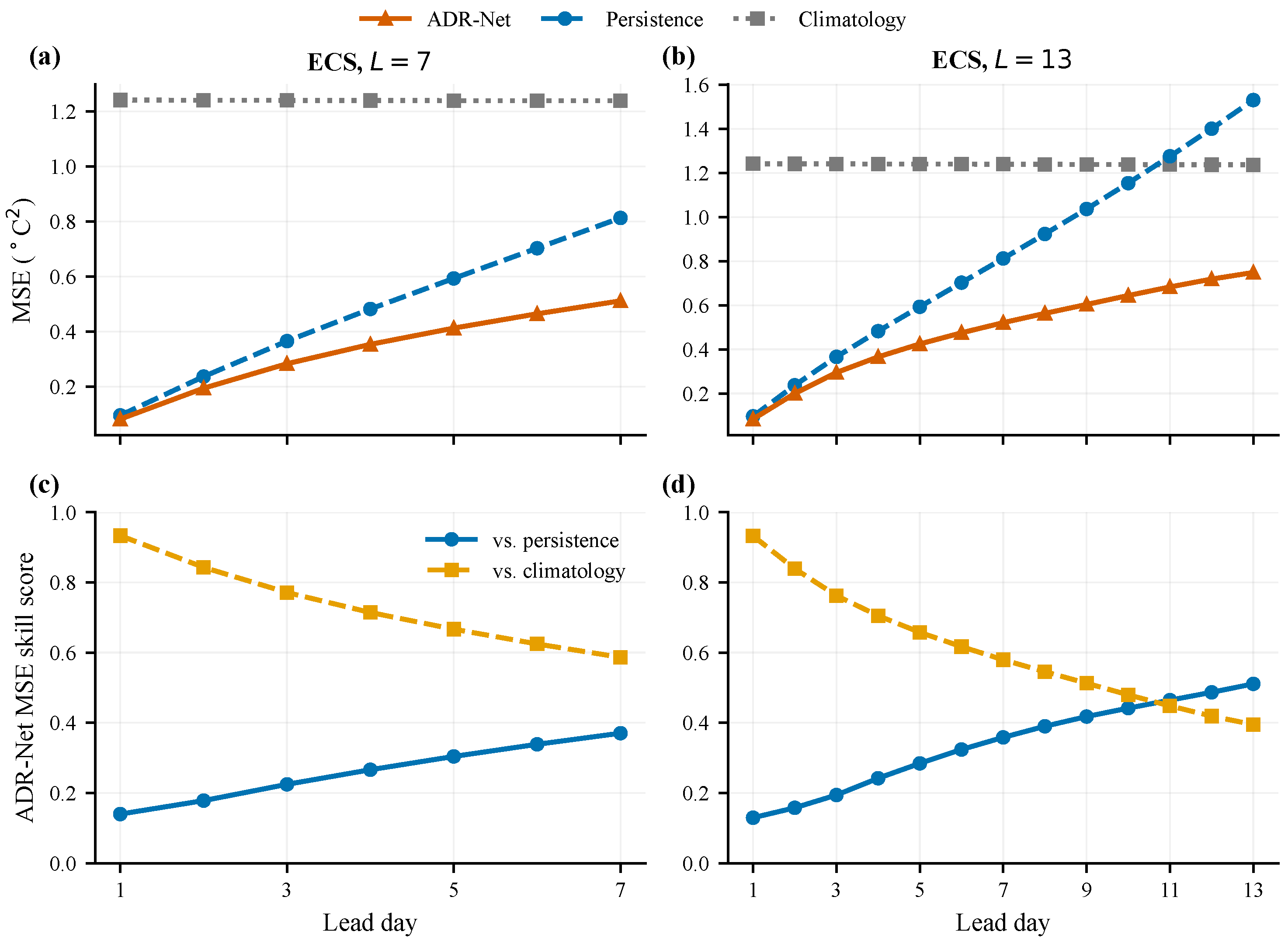
Figure A2 compares ADR-Net with persistence and climatology at each forecast lead for the ECS $L=7$ and $L=13$ forecasting tasks. The persistence-relative skill increases with the lead time because persistence errors grow more rapidly as the latest observed SST field becomes less representative of the future state. In contrast, climatology errors remain nearly lead-independent because this reference depends on the target calendar day rather than the forecast initialization. The decreasing but positive climatology-relative curves therefore reflect the increasing ADR-Net forecast error with the lead time, while retaining a lower MSE than climatology.

Figure A2. Leadwise comparison of ADR-Net with persistence and climatology in the ECS. Panels (a,b) report the MSE for the independently trained $L=7$ and $L=13$ models, respectively; panels (c,d) report the corresponding MSE skill scores. The skill scores remain positive at every available lead, showing that ADR-Net has a lower leadwise MSE than both references throughout the ECS seven- and 13-day forecasts. The $L=1$ setting contains only one lead and is summarized in Figure A1.

Figure A2. Leadwise comparison of ADR-Net with persistence and climatology in the ECS. Panels (a,b) report the MSE for the independently trained $L=7$ and $L=13$ models, respectively; panels (c,d) report the corresponding MSE skill scores. The skill scores remain positive at every available lead, showing that ADR-Net has a lower leadwise MSE than both references throughout the ECS seven- and 13-day forecasts. The $L=1$ setting contains only one lead and is summarized in Figure A1.

Appendix A.2. Multi-Event Evaluation of Storm-Associated SST Cooling

To extend the single-grid-cell, one-day-ahead analysis of Typhoon In-fa, we evaluated regional SST forecasts over four storm-associated episodes: In-fa, Aere, Songda–Trases, and Hinnamnor–Muifa. This supplementary analysis used the independently trained ECS models with an output length of 13 days and examined all forecast leads from day 1 to day 13. The 2022 passage windows were identified from IBTrACS main-track records [37]; the In-fa interval follows the event documentation used in the main-text case study [36]. Closely spaced storms were grouped into episodes to account for overlapping SST responses. All methods were evaluated using matched target dates, forecast leads, and grid cells.

For each episode, SST anomalies were calculated relative to the grid cell mean over the seven days preceding the passage interval. The evaluation window extended from the first passage date to 14 days after the final passage date. Grid cells with an observed anomaly at or below −0.5 °C on at least one day within this window formed the cooling footprint (Table A1). The MAE was calculated from the absolute grid cell errors over the cooling footprint and, separately, over the entire ECS. Event-level errors were averaged across forecast leads, and the four episodes received equal weight in the aggregate comparisons.

ADR-Net achieved the lowest event-mean cooling footprint MAE, 0.553 °C, compared with 0.621 °C for the strongest aggregate baseline, SimVP, corresponding to an 11.0% reduction (Figure A3a). Over the entire ECS, its MAE was 0.571 °C, compared with 0.622 °C for Earthformer—a reduction of 8.2%. ADR-Net also maintained the lowest event-mean cooling footprint MAE at every forecast lead from day 1 to day 13 (Figure A3b), demonstrating that its aggregate advantage extends across the forecast sequence. At the event level, ADR-Net ranked first for Aere and Songda–Trases and remained close to the best result for In-fa, whereas the baselines performed better for Hinnamnor–Muifa.

Table A1. Storm episodes and observed cooling footprints used in the multi-event analysis. The pre-passage baseline is the grid cell mean over the seven days before the passage interval. The evaluation window extends from the first passage date to 14 days after the final passage date. A cooling footprint cell reaches an anomaly of at most −0.5 °C at least once in this window. The minimum anomaly is calculated from the latitude-weighted mean over the corresponding footprint.

Episode	Passage Interval	Footprint Cells (Domain %)	Minimum Area-Mean Anomaly (°C)
Typhoon In-fa	22–27 July 2021	1308 (92.9)	$-1.271$
Aere	2–4 July 2022	122 (8.7)	$-0.572$
Songda–Trases	29 July–1 August 2022	462 (32.8)	$-0.554$
Hinnamnor–Muifa	31 August–14 September 2022	1408 (100.0)	$-2.668$

Table A1. Storm episodes and observed cooling footprints used in the multi-event analysis. The pre-passage baseline is the grid cell mean over the seven days before the passage interval. The evaluation window extends from the first passage date to 14 days after the final passage date. A cooling footprint cell reaches an anomaly of at most −0.5 °C at least once in this window. The minimum anomaly is calculated from the latitude-weighted mean over the corresponding footprint.

Episode	Passage Interval	Footprint Cells (Domain %)	Minimum Area-Mean Anomaly (°C)
Typhoon In-fa	22–27 July 2021	1308 (92.9)	$-1.271$
Aere	2–4 July 2022	122 (8.7)	$-0.572$
Songda–Trases	29 July–1 August 2022	462 (32.8)	$-0.554$
Hinnamnor–Muifa	31 August–14 September 2022	1408 (100.0)	$-2.668$

To assess tracking after cooling emerged, the observed onset was defined as the first of two consecutive days with a latitude-weighted cooling footprint mean anomaly at or below −0.5 °C. Forecasts initialized on or after this onset date were evaluated over the available leads through the end of the event window. Errors were averaged across initializations within each episode and subsequently across episodes. ADR-Net achieved the lowest post-onset MAE over both spatial domains (Figure A3c). Its cooling footprint MAE was 0.366 °C, compared with 0.411 °C for Earthformer, representing an 11.0% reduction. Over the entire ECS, the corresponding errors were 0.368 and 0.431 °C—a reduction of 14.7%. These results demonstrate its strength in tracking SST evolution once cooling is represented in the observed history.

Onset anticipation was evaluated using pre-onset initializations for which both the observed onset day and the following confirmation day fell within the 13-day forecast window, yielding 12 initializations per episode and 48 in total. A detection required the predicted footprint mean anomaly to remain at or below the onset threshold for two consecutive days. ADR-Net predicted sustained threshold crossings in seven initializations (14.6%); the remaining 41 initializations had no sustained crossing within the forecast window (Figure A3d). The detection counts were 0/12 for In-fa, 0/12 for Aere, 5/12 for Songda–Trases, and 2/12 for Hinnamnor–Muifa. The median absolute onset-time error among the seven detections was four days. This diagnostic characterizes advance onset detection separately from post-onset tracking.

Appendix A.3. Statistical Uncertainty for the ECS 13-Day Forecasting Task

We quantified test-period sampling uncertainty in the ECS $L=13$ model comparisons using the complete paired prediction archive. For each of the 2167 chronologically ordered test sequences, the MSE and MAE were calculated over all 13 forecast leads and the $44\times 32$ spatial grid. The aggregate RMSE was obtained as the square root of the aggregate MSE. We applied a non-circular moving-block percentile bootstrap with 30-day blocks and 10,000 resamples, using the same resampled temporal blocks for every model to preserve pairing. The resulting 95% confidence intervals describe test-period sampling uncertainty conditional on the fixed trained models and their saved predictions.

ADR-Net had the lowest point estimates for all three error metrics (Table A2). To quantify its error advantage over each learned baseline, we calculated the bootstrap distribution of the paired difference

$$\Delta M=M_{\mathrm{baseline}}-M_{\mathrm{ADR-Net}},$$

where a positive value indicates a lower error for ADR-Net.

Figure A3. Multi-event evaluation of storm-associated sea surface temperature (SST) cooling in the East China Sea (ECS). (a) Cooling footprint mean absolute error (MAE) for each episode, averaged over forecast leads 1–13, and the equally weighted event mean. Outlined bold entries identify the lowest error in each column. (b) Event-mean cooling footprint MAE at each forecast lead. Pale curves represent individual baselines; the dashed curve selects the lowest baseline error separately at each lead. (c) Post-onset MAE over the cooling footprint (filled circles) and the entire ECS (open squares), with equal event weighting. Connecting segments pair the two spatial domains. (d) ADR-Net onset detection for initializations one to 12 days before observed onset. Crosses indicate no sustained threshold crossing within the forecast window. Signed numbers denote predicted minus observed onset date in days, with negative and positive values indicating early and late predictions, respectively. Counts on the right report detections among the 12 initializations for each episode. The median absolute timing error among the seven detections was four days. Onset is defined as the first of two consecutive days with a latitude-weighted footprint mean anomaly at or below −0.5 °C relative to the seven-day pre-passage reference.

Figure A3. Multi-event evaluation of storm-associated sea surface temperature (SST) cooling in the East China Sea (ECS). (a) Cooling footprint mean absolute error (MAE) for each episode, averaged over forecast leads 1–13, and the equally weighted event mean. Outlined bold entries identify the lowest error in each column. (b) Event-mean cooling footprint MAE at each forecast lead. Pale curves represent individual baselines; the dashed curve selects the lowest baseline error separately at each lead. (c) Post-onset MAE over the cooling footprint (filled circles) and the entire ECS (open squares), with equal event weighting. Connecting segments pair the two spatial domains. (d) ADR-Net onset detection for initializations one to 12 days before observed onset. Crosses indicate no sustained threshold crossing within the forecast window. Signed numbers denote predicted minus observed onset date in days, with negative and positive values indicating early and late predictions, respectively. Counts on the right report detections among the 12 initializations for each episode. The median absolute timing error among the seven detections was four days. Onset is defined as the first of two consecutive days with a latitude-weighted footprint mean anomaly at or below −0.5 °C relative to the seven-day pre-passage reference.

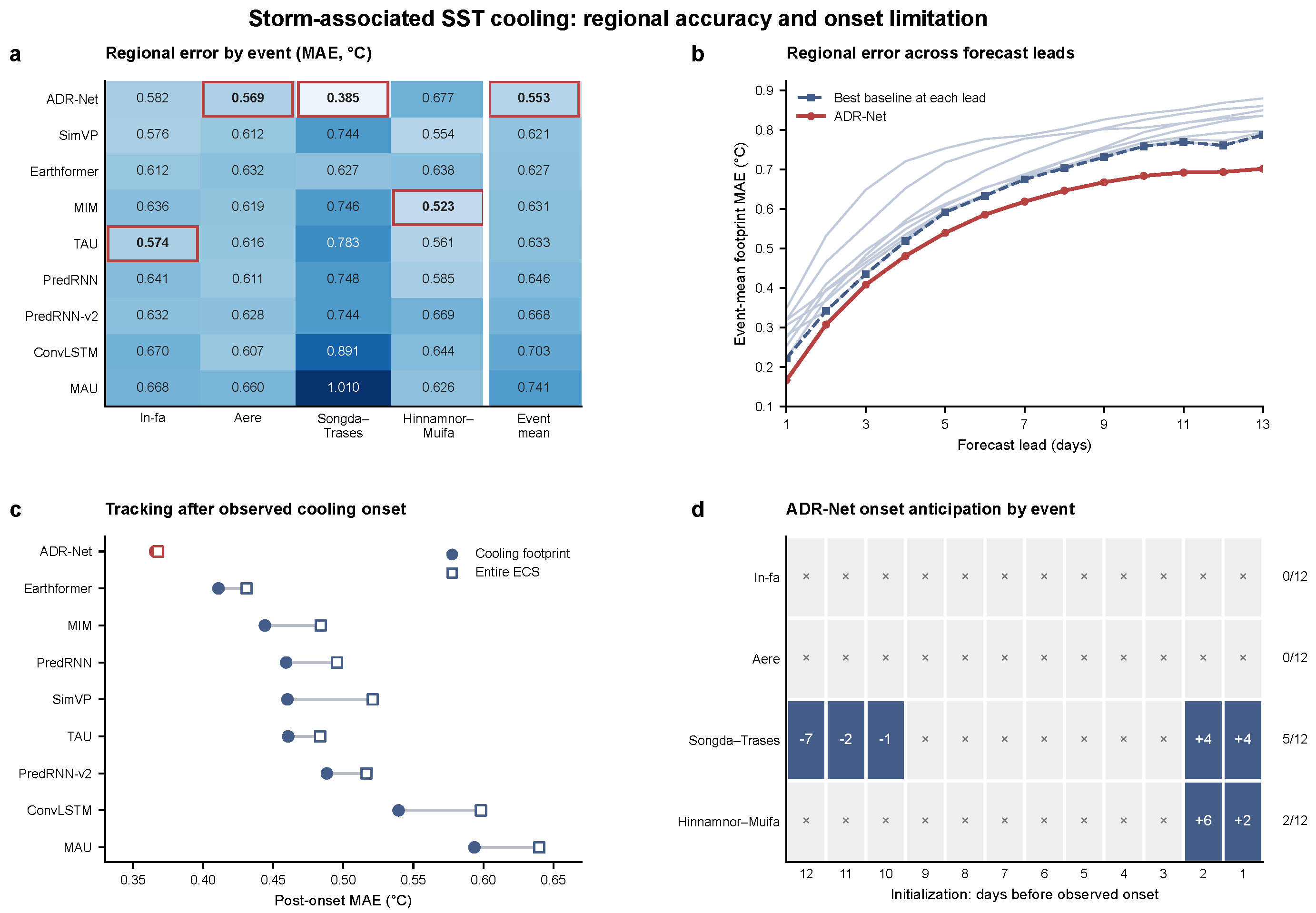
Table A2. Aggregate errors and 95% moving-block bootstrap confidence intervals for the East China Sea (ECS) 13-day forecasting task. Each estimate aggregates all 2167 test sequences, 13 forecast leads, and spatial grid cells. MSE denotes mean squared error, MAE denotes mean absolute error, and RMSE denotes root mean squared error. MSE is reported in (°C)²; MAE and RMSE are reported in °C.

Model	MSE [95% CI]	MAE [95% CI]	RMSE [95% CI]
ADR-Net	0.4868 [0.4415, 0.5363]	0.5040 [0.4795, 0.5302]	0.6977 [0.6645, 0.7323]
SimVP	0.5162 [0.4668, 0.5693]	0.5368 [0.5085, 0.5668]	0.7185 [0.6832, 0.7545]
PredRNN	0.5636 [0.5163, 0.6152]	0.5599 [0.5351, 0.5865]	0.7507 [0.7186, 0.7843]
TAU	0.5603 [0.5126, 0.6169]	0.5600 [0.5344, 0.5898]	0.7486 [0.7159, 0.7854]
PredRNN-v2	0.5922 [0.5398, 0.6525]	0.5693 [0.5429, 0.5990]	0.7695 [0.7347, 0.8078]
Earthformer	0.5706 [0.5227, 0.6205]	0.5710 [0.5451, 0.5976]	0.7554 [0.7230, 0.7877]
MIM	0.6059 [0.5580, 0.6567]	0.5834 [0.5589, 0.6093]	0.7784 [0.7470, 0.8103]
ConvLSTM	0.6442 [0.5889, 0.7058]	0.6059 [0.5785, 0.6358]	0.8026 [0.7674, 0.8401]
MAU	0.6477 [0.5964, 0.7057]	0.6107 [0.5840, 0.6408]	0.8048 [0.7723, 0.8401]

Table A2. Aggregate errors and 95% moving-block bootstrap confidence intervals for the East China Sea (ECS) 13-day forecasting task. Each estimate aggregates all 2167 test sequences, 13 forecast leads, and spatial grid cells. MSE denotes mean squared error, MAE denotes mean absolute error, and RMSE denotes root mean squared error. MSE is reported in (°C)²; MAE and RMSE are reported in °C.

Model	MSE [95% CI]	MAE [95% CI]	RMSE [95% CI]
ADR-Net	0.4868 [0.4415, 0.5363]	0.5040 [0.4795, 0.5302]	0.6977 [0.6645, 0.7323]
SimVP	0.5162 [0.4668, 0.5693]	0.5368 [0.5085, 0.5668]	0.7185 [0.6832, 0.7545]
PredRNN	0.5636 [0.5163, 0.6152]	0.5599 [0.5351, 0.5865]	0.7507 [0.7186, 0.7843]
TAU	0.5603 [0.5126, 0.6169]	0.5600 [0.5344, 0.5898]	0.7486 [0.7159, 0.7854]
PredRNN-v2	0.5922 [0.5398, 0.6525]	0.5693 [0.5429, 0.5990]	0.7695 [0.7347, 0.8078]
Earthformer	0.5706 [0.5227, 0.6205]	0.5710 [0.5451, 0.5976]	0.7554 [0.7230, 0.7877]
MIM	0.6059 [0.5580, 0.6567]	0.5834 [0.5589, 0.6093]	0.7784 [0.7470, 0.8103]
ConvLSTM	0.6442 [0.5889, 0.7058]	0.6059 [0.5785, 0.6358]	0.8026 [0.7674, 0.8401]
MAU	0.6477 [0.5964, 0.7057]	0.6107 [0.5840, 0.6408]	0.8048 [0.7723, 0.8401]

The paired 95% confidence intervals for the baseline-minus-ADR-Net differences were above zero for all eight learned baselines and all three metrics (Table A3). This included SimVP, the strongest aggregate baseline in the ECS $L=13$ task. Repeating the bootstrap analysis with 13- and 60-day blocks preserved this result, showing that the paired error advantage was consistent across the three examined block lengths.

Table A3. Paired error differences between each learned baseline and ADR-Net for the ECS $L=13$ task. Values are the baseline error minus the ADR-Net error, followed by the 95% moving-block bootstrap confidence interval. Positive intervals indicate lower test-period errors for ADR-Net. CI denotes confidence interval; the other metric abbreviations are defined in Table A2.

Baseline	ΔMSE [95% CI]	ΔMAE [95% CI]	ΔRMSE [95% CI]
SimVP	0.0294 [0.0031, 0.0586]	0.0328 [0.0176, 0.0506]	0.0208 [0.0022, 0.0411]
PredRNN	0.0768 [0.0574, 0.0981]	0.0559 [0.0454, 0.0685]	0.0530 [0.0395, 0.0675]
TAU	0.0735 [0.0483, 0.1037]	0.0560 [0.0425, 0.0730]	0.0508 [0.0335, 0.0710]
PredRNN-v2	0.1054 [0.0753, 0.1419]	0.0653 [0.0496, 0.0847]	0.0718 [0.0517, 0.0953]
Earthformer	0.0838 [0.0510, 0.1162]	0.0671 [0.0479, 0.0862]	0.0576 [0.0349, 0.0802]
MIM	0.1191 [0.0885, 0.1493]	0.0795 [0.0637, 0.0959]	0.0807 [0.0598, 0.1013]
ConvLSTM	0.1574 [0.1292, 0.1907]	0.1019 [0.0875, 0.1197]	0.1049 [0.0869, 0.1252]
MAU	0.1609 [0.1303, 0.1987]	0.1068 [0.0898, 0.1285]	0.1071 [0.0867, 0.1315]

Table A3. Paired error differences between each learned baseline and ADR-Net for the ECS $L=13$ task. Values are the baseline error minus the ADR-Net error, followed by the 95% moving-block bootstrap confidence interval. Positive intervals indicate lower test-period errors for ADR-Net. CI denotes confidence interval; the other metric abbreviations are defined in Table A2.

Baseline	ΔMSE [95% CI]	ΔMAE [95% CI]	ΔRMSE [95% CI]
SimVP	0.0294 [0.0031, 0.0586]	0.0328 [0.0176, 0.0506]	0.0208 [0.0022, 0.0411]
PredRNN	0.0768 [0.0574, 0.0981]	0.0559 [0.0454, 0.0685]	0.0530 [0.0395, 0.0675]
TAU	0.0735 [0.0483, 0.1037]	0.0560 [0.0425, 0.0730]	0.0508 [0.0335, 0.0710]
PredRNN-v2	0.1054 [0.0753, 0.1419]	0.0653 [0.0496, 0.0847]	0.0718 [0.0517, 0.0953]
Earthformer	0.0838 [0.0510, 0.1162]	0.0671 [0.0479, 0.0862]	0.0576 [0.0349, 0.0802]
MIM	0.1191 [0.0885, 0.1493]	0.0795 [0.0637, 0.0959]	0.0807 [0.0598, 0.1013]
ConvLSTM	0.1574 [0.1292, 0.1907]	0.1019 [0.0875, 0.1197]	0.1049 [0.0869, 0.1252]
MAU	0.1609 [0.1303, 0.1987]	0.1068 [0.0898, 0.1285]	0.1071 [0.0867, 0.1315]

Appendix A.4. External Evaluation Against iQuam In Situ SST

We matched the ECS $L=13$ forecasts to quality-5 iQuam V2.10 observations as described in Section 2.1. The aggregate MAE, RMSE, and bias were calculated by pooling all matched forecast–observation pairs, giving equal weight to each matched record. For the paired comparisons, the absolute errors were first averaged over all matched records on each UTC date. We then calculated the baseline-minus-ADR-Net daily MAE differences and averaged them with equal weight across dates with valid paired observations. Confidence intervals were obtained using a paired non-circular moving-block percentile bootstrap with blocks of 30 consecutive valid observation days and 10,000 resamples.

Table A4 summarizes the aggregate MAE, RMSE, and bias against quality-5 iQuam observations for all matched platforms and the subset of two fixed coastal moorings. The all-platform evaluation included 493,499 matched forecast–observation pairs for each method, with each pair corresponding to a forecast lead and a platform-day observation. ADR-Net had the lowest learned-model MAE (0.7704 °C) and RMSE (1.0126 °C), and it ranked first among the nine learned models at all 13 leads for both metrics. Relative to ADR-Net, the paired daily MAE differences for every learned baseline had 95% moving-block bootstrap intervals above zero; for the closest baseline, SimVP, the difference was 0.0248 °C [0.0085, 0.0426].

Table A4. External ECS $L=13$ evaluation against quality-5 iQuam V2.10 observations. Metrics pool matched forecast leads and platform days. The fixed coastal-moored subset contains two platforms. OISST v2.1 is included as analysis context and is excluded from learned-model ranks. Bias is prediction minus iQuam. All values are in °C.

	All Quality-5 Platforms			Fixed Coastal Moorings
Method	MAE	RMSE	Bias	MAE	RMSE	Bias
OISST v2.1 analysis	0.6062	0.8281	−0.0941	0.5438	0.6890	0.3428
ADR-Net	0.7704	1.0126	−0.1012	0.8971	1.2082	0.4157
SimVP	0.7953	1.0357	−0.1537	0.9515	1.2320	0.3499
PredRNN	0.8038	1.0484	−0.1468	0.9702	1.3100	0.3740
TAU	0.8064	1.0512	−0.2817	0.8251	1.1388	0.1102
PredRNN-v2	0.8163	1.0604	−0.1853	0.9691	1.2984	0.3533
Earthformer	0.8053	1.0470	−0.1252	1.1063	1.3814	0.4576
MIM	0.8212	1.0644	−0.1687	1.0317	1.3090	0.3848
ConvLSTM	0.8367	1.0874	−0.1733	1.0971	1.4344	0.4906
MAU	0.8299	1.0759	−0.2115	1.0499	1.3508	0.3150

Table A4. External ECS $L=13$ evaluation against quality-5 iQuam V2.10 observations. Metrics pool matched forecast leads and platform days. The fixed coastal-moored subset contains two platforms. OISST v2.1 is included as analysis context and is excluded from learned-model ranks. Bias is prediction minus iQuam. All values are in °C.

	All Quality-5 Platforms			Fixed Coastal Moorings
Method	MAE	RMSE	Bias	MAE	RMSE	Bias
OISST v2.1 analysis	0.6062	0.8281	−0.0941	0.5438	0.6890	0.3428
ADR-Net	0.7704	1.0126	−0.1012	0.8971	1.2082	0.4157
SimVP	0.7953	1.0357	−0.1537	0.9515	1.2320	0.3499
PredRNN	0.8038	1.0484	−0.1468	0.9702	1.3100	0.3740
TAU	0.8064	1.0512	−0.2817	0.8251	1.1388	0.1102
PredRNN-v2	0.8163	1.0604	−0.1853	0.9691	1.2984	0.3533
Earthformer	0.8053	1.0470	−0.1252	1.1063	1.3814	0.4576
MIM	0.8212	1.0644	−0.1687	1.0317	1.3090	0.3848
ConvLSTM	0.8367	1.0874	−0.1733	1.0971	1.4344	0.4906
MAU	0.8299	1.0759	−0.2115	1.0499	1.3508	0.3150

The evaluation at two fixed coastal moorings included 9633 matched forecast–observation pairs for each method, with observations concentrated in 2021–2022. ADR-Net ranked second in the MAE and RMSE, following TAU. The paired daily MAE difference, defined as TAU minus ADR-Net, was −0.0657 °C, with a 95% confidence interval of $[-0.1656,0.0532]$, indicating no statistically resolved difference in the daily MAE between the two models in this coastal subset.

Appendix A.5. Forecast Accuracy and Structural Similarity Across Output Lengths

Figure A4 compares the per-lead MSE and SSIM for the ECS tasks with $L=1$, 7, and 13. These metrics characterize the prediction errors and spatial structure preservation over the forecast leads available in each task.

Figure A4. Forecast accuracy and structural similarity of ECS models trained separately for each output length. Panels (a–c) show the per-lead mean squared error (MSE) for $L=1$, 7, and 13, respectively; panels (d–f) show the corresponding structural similarity index (SSIM). Lower MSE and higher SSIM indicate better performance.

Figure A4. Forecast accuracy and structural similarity of ECS models trained separately for each output length. Panels (a–c) show the per-lead mean squared error (MSE) for $L=1$, 7, and 13, respectively; panels (d–f) show the corresponding structural similarity index (SSIM). Lower MSE and higher SSIM indicate better performance.

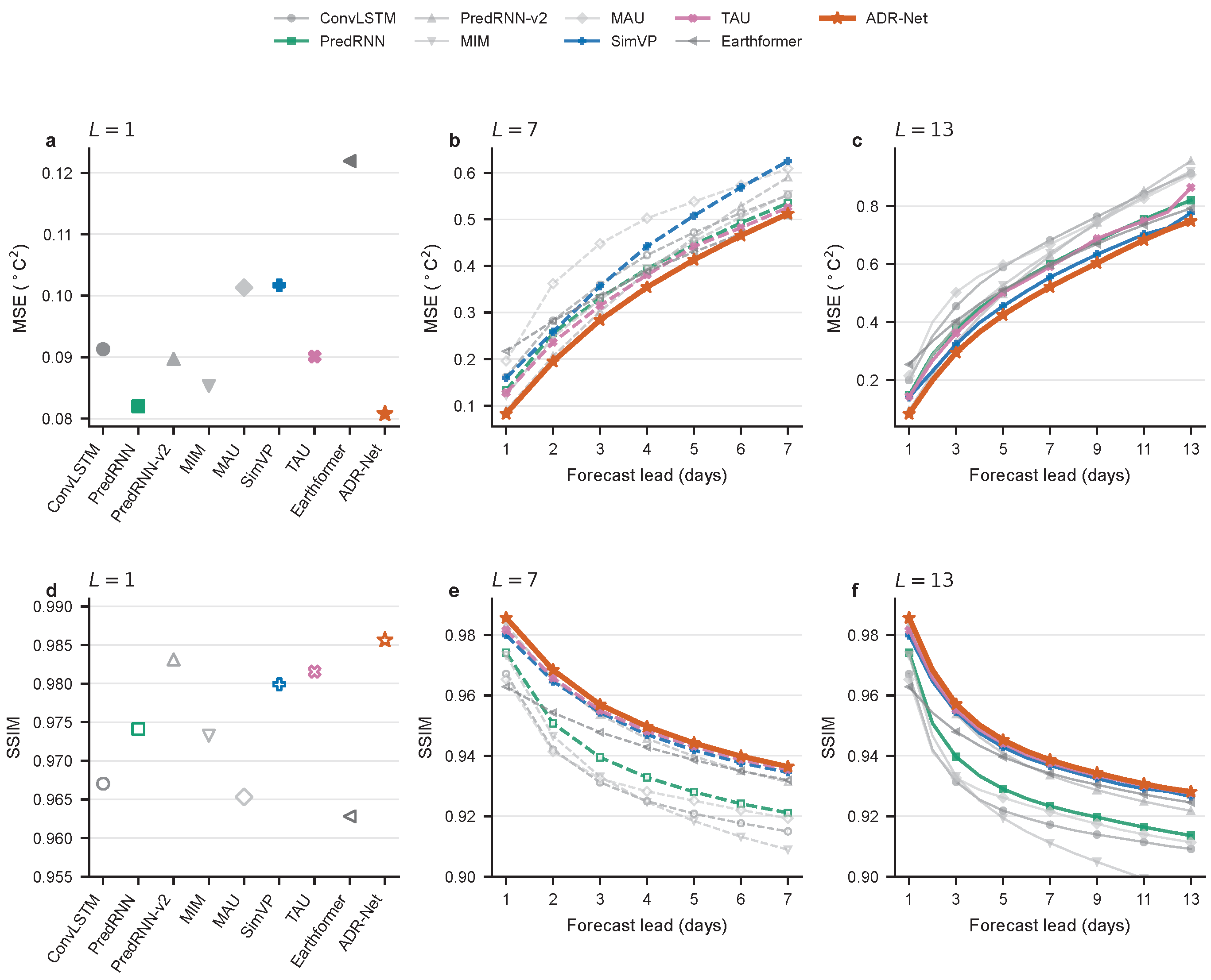
ADR-Net achieved the highest SSIM at every available forecast lead in the three independently trained ECS tasks (Figure A4d–f). The per-lead curves show that its spatial structure advantage persists throughout the forecast sequences for both multi-step output lengths.

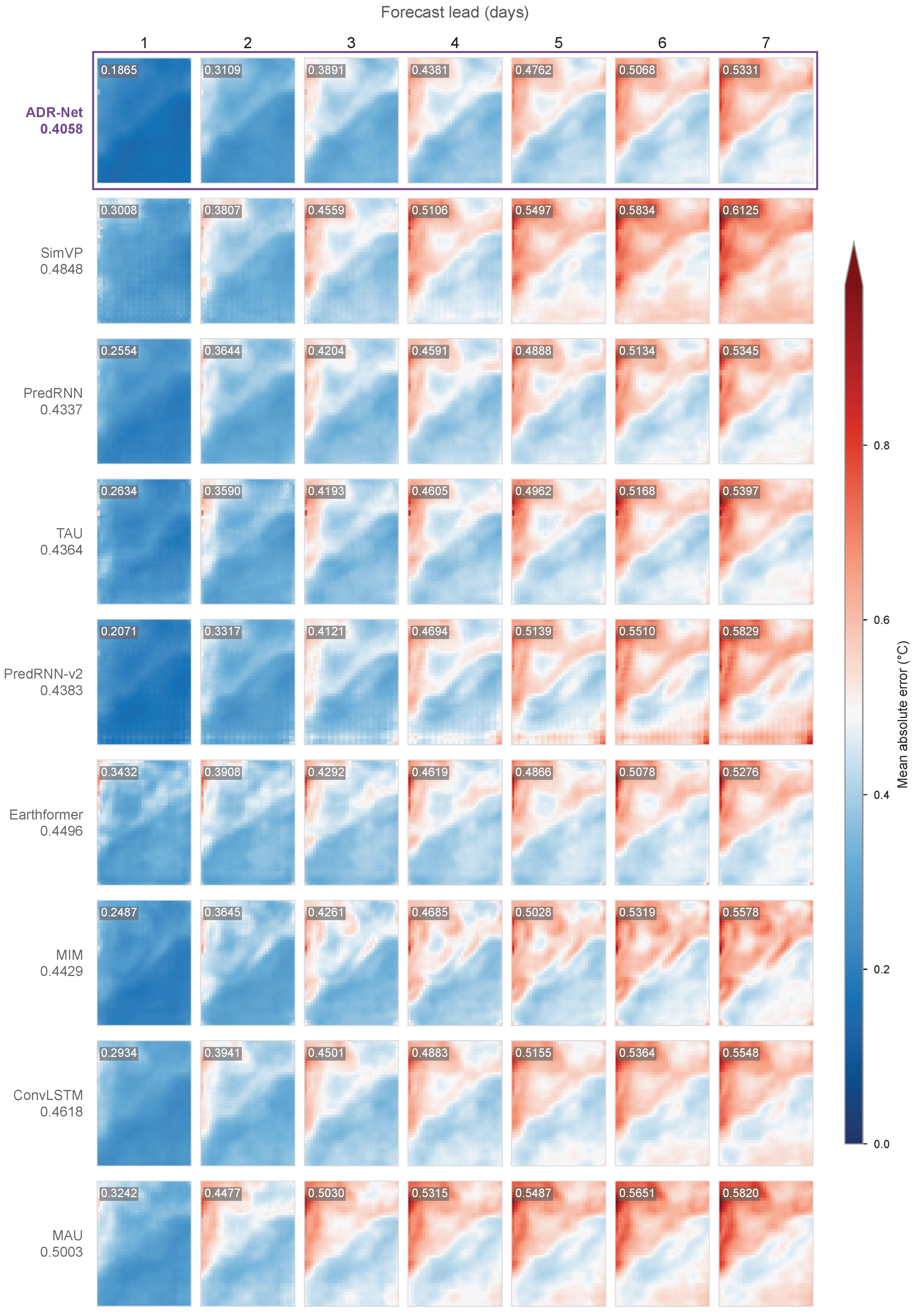
Figure A5 and Figure A6 resolve the corresponding errors spatially. In the one-day task, ADR-Net exhibited low absolute errors over most grid cells. Across the seven-day sequence, it maintained comparatively low and spatially uniform errors, while several baselines developed broader high-error regions at the middle and later leads. These maps identify the spatial distribution of the accuracy differences summarized in Table 3.

Figure A5. Spatial distributions of mean absolute error (MAE) for the independently trained ECS $L=1$ models. Each panel corresponds to one model, and the value in the upper-left corner denotes its aggregate test-set MAE. All models share the same linear color scale, with lighter and redder colors indicating larger errors; the purple outline identifies ADR-Net.

Figure A5. Spatial distributions of mean absolute error (MAE) for the independently trained ECS $L=1$ models. Each panel corresponds to one model, and the value in the upper-left corner denotes its aggregate test-set MAE. All models share the same linear color scale, with lighter and redder colors indicating larger errors; the purple outline identifies ADR-Net.

Figure A6. Spatial distributions of mean absolute error (MAE) over forecast leads 1–7 for the independently trained ECS $L=7$ models. Rows correspond to models, and columns correspond to forecast leads. The value in the upper-left corner of each panel denotes the spatially averaged MAE at that lead, whereas the value below each model name denotes the aggregate MAE across the seven-lead sequence. All panels share the same linear color scale, with lighter and redder colors indicating larger errors; the purple outline identifies ADR-Net.

Figure A6. Spatial distributions of mean absolute error (MAE) over forecast leads 1–7 for the independently trained ECS $L=7$ models. Rows correspond to models, and columns correspond to forecast leads. The value in the upper-left corner of each panel denotes the spatially averaged MAE at that lead, whereas the value below each model name denotes the aggregate MAE across the seven-lead sequence. All panels share the same linear color scale, with lighter and redder colors indicating larger errors; the purple outline identifies ADR-Net.

References

- O’Carroll, A.G.; Armstrong, E.M.; Beggs, H.M.; Bouali, M.; Casey, K.S.; Corlett, G.K.; Dash, P.; Donlon, C.J.; Gentemann, C.L.; Høyer, J.L.; et al. Observational Needs of Sea Surface Temperature. Front. Mar. Sci. 2019, 6, 420. [Google Scholar] [CrossRef] [Scilit]
- Minnett, P.J.; Alvera-Azcárate, A.; Chin, T.M.; Corlett, G.K.; Gentemann, C.L.; Karagali, I.; Li, X.; Marsouin, A.; Marullo, S.; Maturi, E.; et al. Half a Century of Satellite Remote Sensing of Sea-Surface Temperature. Remote Sens. Environ. 2019, 233, 111366. [Google Scholar] [CrossRef] [Scilit]
- Pasquero, C.; Desbiolles, F.; Meroni, A.N. Air–Sea Interactions in the Cold Wakes of Tropical Cyclones. Geophys. Res. Lett. 2021, 48, e2020GL091185. [Google Scholar] [CrossRef] [Scilit]
- Yang, H.; Cao, J.; Li, W.; Wang, S.; Li, H.; Guan, J.; Zhou, S. Spatial-Temporal Data Mining for Ocean Science: Data, Methodologies, and Opportunities. ACM Trans. Knowl. Discov. Data 2025, 19, 140. [Google Scholar] [CrossRef] [Scilit]
- Yang, Y.; Dong, J.; Sun, X.; Lima, E.; Mu, Q.; Wang, X. A CFCC-LSTM Model for Sea Surface Temperature Prediction. IEEE Geosci. Remote Sens. Lett. 2018, 15, 207–211. [Google Scholar] [CrossRef] [Scilit]
- Xiao, C.; Chen, N.; Hu, C.; Wang, K.; Xu, Z.; Cai, Y.; Xu, L.; Chen, Z.; Gong, J. A Spatiotemporal Deep Learning Model for Sea Surface Temperature Field Prediction Using Time-Series Satellite Data. Environ. Model. Softw. 2019, 120, 104502. [Google Scholar] [CrossRef] [Scilit]
- Ren, J.; Wang, C.; Sun, L.; Huang, B.; Zhang, D.; Mu, J.; Wu, J. Prediction of Sea Surface Temperature Using U-Net Based Model. Remote Sens. 2024, 16, 1205. [Google Scholar] [CrossRef] [Scilit]
- Shi, B.; Ge, C.; Lin, H.; Xu, Y.; Tan, Q.; Peng, Y.; He, H. Sea Surface Temperature Prediction Using ConvLSTM-Based Model with Deformable Attention. Remote Sens. 2024, 16, 4126. [Google Scholar] [CrossRef] [Scilit]
- Yang, H.; Li, W.; Hou, S.; Guan, J.; Zhou, S. HiGRN: A Hierarchical Graph Recurrent Network for Global Sea Surface Temperature Prediction. ACM Trans. Intell. Syst. Technol. 2023, 14, 73. [Google Scholar] [CrossRef] [Scilit]
- Peng, H.; Li, W.; Jin, C.; Zhang, Y.; Guan, J.; Yang, H.; Zhou, S. Cross-Region Graph Convolutional Network with Periodicity Shift Adaptation for Wide-Area SST Prediction. ACM Trans. Intell. Syst. Technol. 2025, 16, 87. [Google Scholar] [CrossRef] [Scilit]
- Yang, H.; Chen, Y.; Cao, J.; Li, W.; Yang, Y.; Wang, S.; Guan, J.; Qin, R.; Zhou, S. UniOcean: A Unified Framework for Predicting Multiple Ocean Factors of Varying Temporal Scales. IEEE Trans. Geosci. Remote Sens. 2024, 62, 4213116. [Google Scholar] [CrossRef] [Scilit]
- Yang, H.; Wang, J.; Cao, J.; Li, W.; Zheng, J.; Li, Y.; Miao, C.; Guan, J.; Zhou, S.; Yu, P.S. OKG-LLM: Aligning Ocean Knowledge Graph with Observation Data via LLMs for Global Sea Surface Temperature Prediction. IEEE Trans. Knowl. Data Eng. 2026, 38, 3009–3021. [Google Scholar] [CrossRef] [Scilit]
- Jin, C.; Peng, H.; Yang, H.; Li, W.; Guan, J. On Evaluating the Predictability of Sea Surface Temperature Using Entropy. Remote Sens. 2023, 15, 1956. [Google Scholar] [CrossRef] [Scilit]
- Reichstein, M.; Camps-Valls, G.; Stevens, B.; Jung, M.; Denzler, J.; Carvalhais, N.; Prabhat. Deep Learning and Process Understanding for Data-Driven Earth System Science. Nature 2019, 566, 195–204. [Google Scholar] [CrossRef] [Scilit] [PubMed]
- Karniadakis, G.E.; Kevrekidis, I.G.; Lu, L.; Perdikaris, P.; Wang, S.; Yang, L. Physics-Informed Machine Learning. Nat. Rev. Phys. 2021, 3, 422–440. [Google Scholar] [CrossRef] [Scilit]
- de Bézenac, E.; Pajot, A.; Gallinari, P. Deep Learning for Physical Processes: Incorporating Prior Scientific Knowledge. J. Stat. Mech. Theory Exp. 2019, 2019, 124009. [Google Scholar] [CrossRef] [Scilit]
- Le Guen, V.; Thome, N. Disentangling Physical Dynamics from Unknown Factors for Unsupervised Video Prediction. In Proceedings of the IEEE/CVF Conference on Computer Vision and Pattern Recognition; IEEE: Piscataway, NJ, USA, 2020; pp. 11474–11484. [Google Scholar] [CrossRef] [Scilit]
- Meng, Y.; Gao, F.; Rigall, E.; Dong, R.; Dong, J.; Du, Q. Physical Knowledge-Enhanced Deep Neural Network for Sea Surface Temperature Prediction. IEEE Trans. Geosci. Remote Sens. 2023, 61, 4203013. [Google Scholar] [CrossRef] [Scilit]
- Yuan, T.; Zhu, J.; Wang, W.; Lu, J.; Wang, X.; Li, X.; Ren, K. A Space-Time Partial Differential Equation Based Physics-Guided Neural Network for Sea Surface Temperature Prediction. Remote Sens. 2023, 15, 3498. [Google Scholar] [CrossRef] [Scilit]
- Dong, S.; Li, Y.; Yin, X.; Xu, Q.; Mao, P. Physics-Guided Deep Learning for Global Sea Surface Temperature Forecasting: Balancing Accuracy and Stability across Timescales. Geosci. Front. 2026, 17, 102255. [Google Scholar] [CrossRef] [Scilit]
- Guo, Y.; Song, J.; Cao, X.; Leng, H. A Physics-Guided Hierarchical Transformer Framework for Sea Surface Temperature Forecasting and Marine Heatwave Detection. IEEE Geosci. Remote Sens. Lett. 2026, 23, 1500705. [Google Scholar] [CrossRef] [Scilit]
- Ben Taieb, S.; Bontempi, G.; Atiya, A.F.; Sorjamaa, A. A Review and Comparison of Strategies for Multi-Step Ahead Time Series Forecasting Based on the NN5 Forecasting Competition. Expert Syst. Appl. 2012, 39, 7067–7083. [Google Scholar] [CrossRef] [Scilit]
- Huang, B.; Liu, C.; Banzon, V.; Freeman, E.; Graham, G.; Hankins, B.; Smith, T.; Zhang, H.M. Improvements of the Daily Optimum Interpolation Sea Surface Temperature (DOISST) Version 2.1. J. Clim. 2021, 34, 2923–2939. [Google Scholar] [CrossRef] [Scilit]
- Xu, F.; Ignatov, A. In Situ SST Quality Monitor (iQuam). J. Atmos. Ocean. Technol. 2014, 31, 164–180. [Google Scholar] [CrossRef] [Scilit]
- Paszke, A.; Gross, S.; Massa, F.; Lerer, A.; Bradbury, J.; Chanan, G.; Killeen, T.; Lin, Z.; Gimelshein, N.; Antiga, L.; et al. PyTorch: An Imperative Style, High-Performance Deep Learning Library. In Proceedings of the Advances in Neural Information Processing Systems; Curran Associates, Inc.: Red Hook, NY, USA, 2019; Volume 32, pp. 8024–8035. [Google Scholar]
- Tan, C.; Li, S.; Gao, Z.; Guan, W.; Wang, Z.; Liu, Z.; Wu, L.; Li, S.Z. OpenSTL: A Comprehensive Benchmark of Spatio-Temporal Predictive Learning. In Proceedings of the Advances in Neural Information Processing Systems; Curran Associates, Inc.: Red Hook, NY, USA, 2023; Volume 36, pp. 69819–69831. [Google Scholar] [CrossRef] [Scilit]
- Shi, X.; Chen, Z.; Wang, H.; Yeung, D.Y.; Wong, W.K.; Woo, W.C. Convolutional LSTM Network: A Machine Learning Approach for Precipitation Nowcasting. In Proceedings of the Advances in Neural Information Processing Systems; Curran Associates, Inc.: Red Hook, NY, USA, 2015; Volume 28, pp. 802–810. [Google Scholar]
- Wang, Y.; Long, M.; Wang, J.; Gao, Z.; Yu, P.S. PredRNN: Recurrent Neural Networks for Predictive Learning Using Spatiotemporal LSTMs. In Proceedings of the Advances in Neural Information Processing Systems; Curran Associates, Inc.: Red Hook, NY, USA, 2017; Volume 30, pp. 879–888. [Google Scholar]
- Wang, Y.; Wu, H.; Zhang, J.; Gao, Z.; Wang, J.; Yu, P.S.; Long, M. PredRNN: A Recurrent Neural Network for Spatiotemporal Predictive Learning. IEEE Trans. Pattern Anal. Mach. Intell. 2023, 45, 2208–2225. [Google Scholar] [CrossRef] [Scilit] [PubMed]
- Wang, Y.; Zhang, J.; Zhu, H.; Long, M.; Wang, J.; Yu, P.S. Memory in Memory: A Predictive Neural Network for Learning Higher-Order Non-Stationarity from Spatiotemporal Dynamics. In Proceedings of the IEEE/CVF Conference on Computer Vision and Pattern Recognition; IEEE: Piscataway, NJ, USA, 2019; pp. 9154–9162. [Google Scholar] [CrossRef] [Scilit]
- Chang, Z.; Zhang, X.; Wang, S.; Ma, S.; Ye, Y.; Xiang, X.; Gao, W. MAU: A Motion-Aware Unit for Video Prediction and Beyond. In Proceedings of the Advances in Neural Information Processing Systems; Curran Associates, Inc.: Red Hook, NY, USA, 2021; Volume 34, pp. 26950–26962. [Google Scholar]
- Gao, Z.; Tan, C.; Wu, L.; Li, S.Z. SimVP: Simpler Yet Better Video Prediction. In Proceedings of the IEEE/CVF Conference on Computer Vision and Pattern Recognition; IEEE: Piscataway, NJ, USA, 2022; pp. 3170–3180. [Google Scholar] [CrossRef] [Scilit]
- Tan, C.; Gao, Z.; Wu, L.; Xu, Y.; Xia, J.; Li, S.; Li, S.Z. Temporal Attention Unit: Towards Efficient Spatiotemporal Predictive Learning. In Proceedings of the IEEE/CVF Conference on Computer Vision and Pattern Recognition; IEEE: Piscataway, NJ, USA, 2023; pp. 18770–18782. [Google Scholar] [CrossRef] [Scilit]
- Gao, Z.; Shi, X.; Wang, H.; Zhu, Y.; Wang, Y.; Li, M.; Yeung, D.Y. Earthformer: Exploring Space-Time Transformers for Earth System Forecasting. In Proceedings of the Advances in Neural Information Processing Systems; Curran Associates, Inc.: Red Hook, NY, USA, 2022; Volume 35, pp. 25390–25403. [Google Scholar] [CrossRef] [Scilit]
- Wang, Z.; Bovik, A.C.; Sheikh, H.R.; Simoncelli, E.P. Image Quality Assessment: From Error Visibility to Structural Similarity. IEEE Trans. Image Process. 2004, 13, 600–612. [Google Scholar] [CrossRef] [Scilit] [PubMed]
- Che, Y.; Guo, B.; Mantravadi, V.S.; Wang, J.; Ji, Z. The Impact of Typhoon “In-Fa” (2021) on Temperature, Salinity, and Chlorophyll-a Concentration in the Upwelling Area of Northwestern East China Sea. Atmosphere 2023, 14, 1226. [Google Scholar] [CrossRef] [Scilit]
- NOAA National Centers for Environmental Information. International Best Track Archive for Climate Stewardship (IBTrACS) Project, Version 4.01; Release 1; NOAA National Centers for Environmental Information: Asheville, NC, USA, 2024. [CrossRef]
Disclaimer/Publisher’s Note: The statements, opinions and data contained in all publications are solely those of the individual author(s) and contributor(s) and not of MDPI and/or the editor(s). MDPI and/or the editor(s) disclaim responsibility for any injury to people or property resulting from any ideas, methods, instructions or products referred to in the content. |
© 2026 by the authors. Licensee MDPI, Basel, Switzerland. This article is an open access article distributed under the terms and conditions of the Creative Commons Attribution (CC BY) license.