


Highlights
What are the main findings?
- Fused satellite, meteorology, land use, and landscape data can enhance the accuracy of water quality remote sensing inversion.
- Introduced WOA to auto-optimize ML models, enhancing inversion accuracy and stability.
What are the implications of the main findings?
- Extended water quality inversion from urban to large-scale basins with diverse drivers.
- Integrated landscape pattern indices into models to reveal spatial pollution mechanisms.
Abstract
Accurate and efficient surface water quality monitoring is essential for ecological protection and sustainable development. However, conventional monitoring methods, such as fixed-site observations, often suffer from spatial limitations and overlook crucial auxiliary variables. This study proposes an innovative modeling framework for large-scale river water quality inversion that integrates multi-source data—including Sentinel-2 imagery, meteorological conditions, land use classification, and landscape pattern indices. To improve predictive accuracy, three tree-based machine learning models (Random Forest, XGBoost, and LightGBM) were constructed and further optimized using the Whale Optimization Algorithm (WOA), a nature-inspired metaheuristic technique. Additionally, model interpretability was enhanced using SHAP (Shapley Additive Explanations), enabling a transparent understanding of each variable’s contribution. The framework was applied to the Red River Basin (RRB) to predict six key water quality parameters: dissolved oxygen (DO), ammonia nitrogen (NH3-N), total phosphorus (TP), total nitrogen (TN), pH, and permanganate index (CODMn). Results demonstrate that integrating landscape and meteorological variables significantly improves model performance compared to remote sensing alone. The best-performing models achieved R2 values exceeding 0.45 for all parameters (DO: 0.70, NH3-N: 0.46, TP: 0.59, TN: 0.71, pH: 0.83, CODMn: 0.57). Among them, WOA-optimized LightGBM consistently delivered superior performance. The study also confirms the feasibility of applying the models across the entire basin, offering a transferable and interpretable approach to spatiotemporal water quality prediction in other large-scale or data-scarce regions.
1. Introduction
Surface water plays a vital role in sustaining ecological balance and supporting socioeconomic development [1,2]. However, due to intensifying anthropogenic activities—such as rapid urban expansion and the discharge of untreated domestic wastewater—surface water quality has significantly deteriorated in recent years [3,4,5]. A substantial influx of pollutants into rivers, both directly and indirectly, has led to severe environmental issues, including water blackening, odor generation, and eutrophication. These deteriorations not only compromise the ecological integrity of river systems but also pose serious risks to water security for human consumption and environmental protection. Therefore, effective and timely monitoring of surface water quality is essential to ensure both environmental sustainability and public health [6,7,8].
Surface water quality is typically assessed using various physico-chemical parameters [9,10]. Conventional monitoring methods rely heavily on in situ data collection at fixed stations, which, while accurate, are spatially limited and often expensive to maintain [11,12]. In contrast, advances in remote sensing technologies have greatly improved access to high-resolution and high-frequency multispectral data, enabling broader and more efficient monitoring coverage [13]. Remote sensing-based water quality inversion methods, typically categorized as model-based or empirical approaches, have gained increasing attention [14,15,16]. In addition, machine learning methods have also been used recently due to their high prediction accuracy. Nevertheless, most current studies are concentrated in urban rivers or lakes, where water quality is relatively stable and less influenced by complex upstream interactions [17]. In contrast, large-scale water bodies—characterized by diverse hydrological conditions and heterogeneous human impacts—pose significant challenges for remote sensing inversion due to greater spatial variability.
To address these challenges, machine learning and deep learning techniques have increasingly been adopted for water quality assessment, given their capacity to capture nonlinear and complex relationships between input variables and water quality parameters [18,19,20]. However, most existing machine learning models primarily rely on spectral variables from remote sensing data, often neglecting crucial auxiliary variables such as meteorological conditions, land use, and watershed morphology [21,22]. Yet, environmental variables such as precipitation, temperature, and wind speed significantly influence pollutant transport and biogeochemical processes in river systems [23,24]. Similarly, land use changes—especially the expansion of impervious surfaces—directly alter runoff patterns and pollutant loads [25,26,27]. Moreover, landscape pattern indices, which capture spatial configuration, fragmentation, and connectivity, offer untapped potential for characterizing pollutant dispersion and retention at the watershed scale [28,29,30]. Despite growing evidence of their relevance, these indices have rarely been integrated into water quality model inversion.
To fill this gap, this study proposes an innovative modeling framework that integrates multi-source data—including Sentinel-2 satellite imagery, meteorological variables, land use classification, and landscape pattern metrics—to predict key surface water quality parameters (DO, NH3-N, TP, TN, pH, and CODMn) in the Red River Basin (RRB). We employ three advanced tree-based machine learning algorithms—Random Forest (RF), eXtreme Gradient Boosting (XGBoost), and Light Gradient Boosting Machine (LightGBM)—and enhance their performance through hyperparameter tuning using the Whale Optimization Algorithm (WOA), a nature-inspired metaheuristic technique. Furthermore, we apply SHAP (Shapley Additive Explanations) to interpret the contribution of each input variable, enabling model transparency and ecological insight. The optimized models are validated using historical monitoring station data and applied to generate a spatio-temporal prediction of water quality conditions across the entire RRB in 2023. This research not only demonstrates the effectiveness of multi-source, interpretable machine learning models for large-scale water quality monitoring but also introduces a transferable methodological framework with strong potential for broader applications in hydrological and environmental management.
2. Methods and Materials
2.1. Study Area
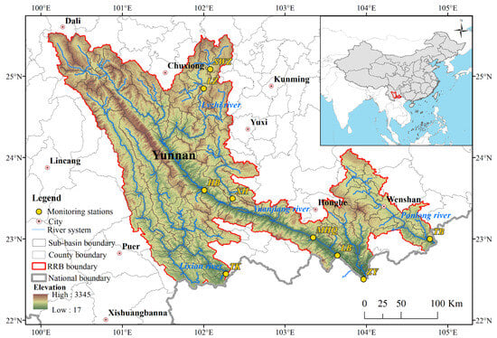
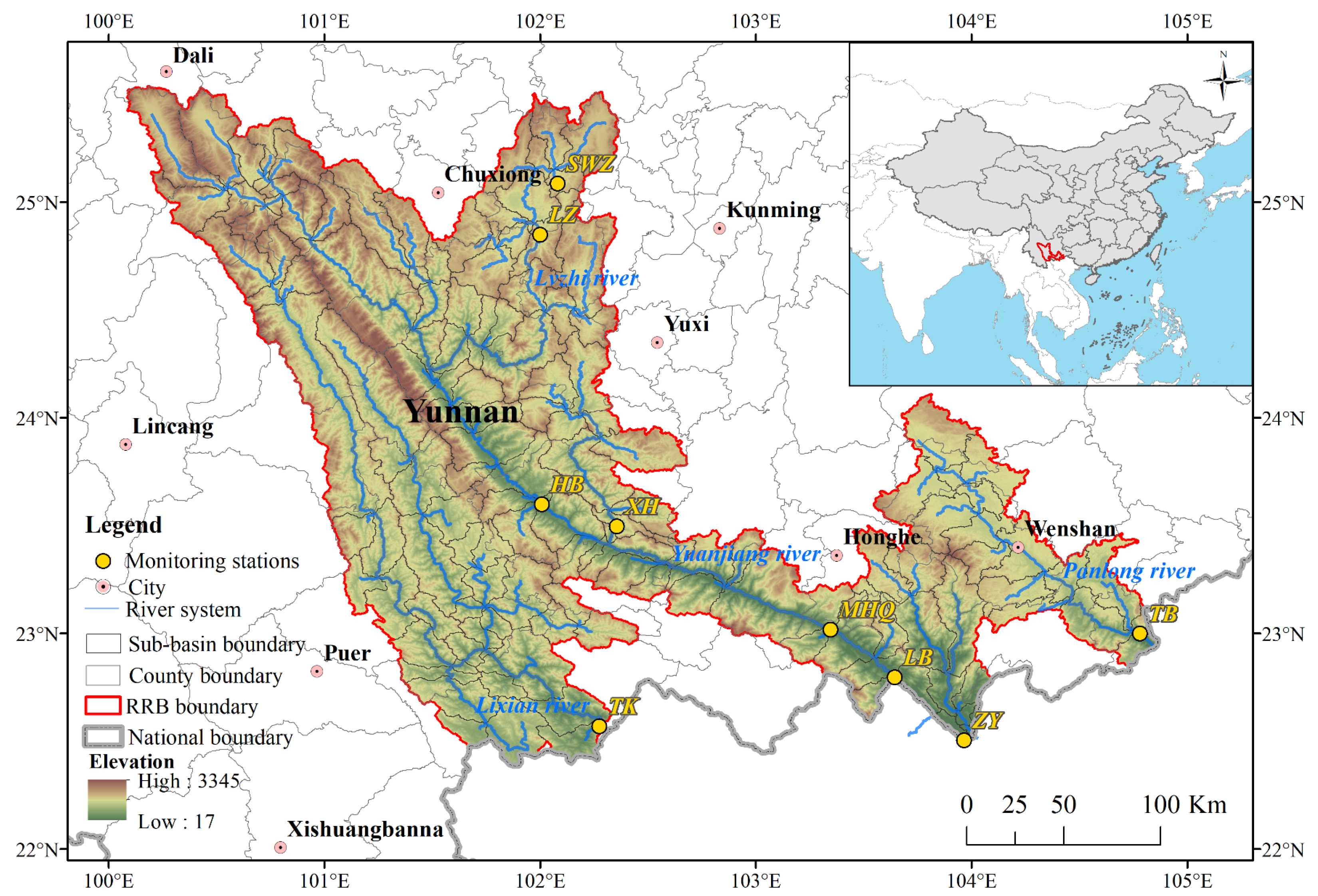
This study is conducted in the RRB (100°04′–104°50′E, 22°23′–25°36′N), which spans an area of approximately 61,700 km2 within the territory of China (Figure 1). The basin features a topography that descends from the highlands in the northwest to the lowlands in the southeast, characterized by significant elevation differences and deeply incised valleys. It experiences a typical subtropical monsoon climate, with distinct wet and dry seasons. The wet season extends from May to October, accounting for over 85% of the annual precipitation, while the dry season lasts from November to April, contributing less than 15% of the annual precipitation [31]. Variations in water quality within the RRB have substantial implications for the ecological integrity and socio-economic development of both upstream and downstream regions.
Figure 1.
Geographical map of the RRB and the spatial distribution of water quality monitoring stations.
2.2. Multi-Source Data
2.2.1. Water Quality Parameters
Water quality parameter data were collected from nine monitoring stations distributed across the RRB and its tributaries (Figure 1) during the period from 2021 to 2023. These data were obtained from the China National Environmental Monitoring Center (www.cnemc.cn), which operates an automated surface water quality monitoring system established by the Ministry of Ecology and Environment of the People’s Republic of China [32]. Measurements were recorded at four-hour intervals, providing high-frequency time series data. In accordance with the national Environmental Quality Standards for Surface Water (GB 3838-2002 [33]) and their relevance to water quality assessment, six key water quality parameters were selected for inversion: pH, dissolved oxygen (DO, mg/L), chemical oxygen demand (CODMn, mg/L), total phosphorus (TP, mg/L), total nitrogen (TN, mg/L), and ammonia nitrogen (NH3-N, mg/L) [3,34]. To address data gaps, linear interpolation was applied to fill a small number of missing values in the in situ water-quality time series, which accounted for 2.6% of the total 60,061 observations. The interpolation process did not result in significant changes in the coefficient of variation for any of the water quality parameter time series (p-value of the two-sided paired t-test is equal to 0.55), thereby preserving their statistical integrity. For consistency with the temporal resolution of remote sensing data, all water quality parameters were aggregated to daily averages for subsequent modeling.
2.2.2. Remote Sensing Data and Preprocessing
Given its high spatial resolution (up to 10 m) and short revisit interval (5 days with the combined operation of two satellites), Sentinel-2 MSI imagery was selected for water quality inversion in this study. Sentinel-2, launched by the European Space Agency, consists of two optical satellites—Sentinel-2A and Sentinel-2B—that collectively provide data across 13 spectral bands. This study utilized Level-2A (L2A) products, which are freely available and have undergone geometric, radiometric, and atmospheric corrections. Due to the unavailability of Band 10 following atmospheric correction, only Bands 1–9, Band 8A, and Bands 11–12 were used for analysis. To minimize the influence of cloud contamination, only images with cloud cover below 10% from 2021 to 2023 were selected. Cloud-masked and filtered imagery was then subjected to further analysis and water quality model inversion.
2.2.3. Meteorological and Land Use Data
Meteorological data spanning from January 2021 to December 2023 were obtained from the China Meteorological Administration. The selected meteorological variables included air temperature (TE, °C), maximum air temperature (MaxTE, °C), minimum air temperature (MinTE, °C), accumulated precipitation (PREC, mm), relative humidity (RHU, %), atmospheric pressure (PRS, hPa), and wind speed (WinS, m/s). All meteorological variables were resampled to a uniform spatial resolution of 500 m using nine interpolation techniques: ordinary kriging, linear interpolation, nearest neighbor interpolation, cubic interpolation, global polynomial interpolation, radial basis function interpolation, local polynomial interpolation, synergistic kriging, and Thiessen (Tyson) polygon interpolation. Land use data for the years 2021–2023, with a spatial resolution of 10 m, were sourced from the Environmental Systems Research Institute (ESRI) Land Cover dataset (https://livingatlas.arcgis.com/landcover/, accessed on 16 September 2025). The dataset includes classification into nine land use categories: water, trees, flooded vegetation, crops, built area, bare ground, snow/ice, and rangeland [35]. These variables were used to assess the impact of land surface conditions on water quality dynamics within the study area.
2.2.4. Landscape Pattern Indices
The landscape pattern indices provide insights into the spatial distribution characteristics of different land cover types within the basin. Although these indices do not directly measure water quality, they are closely associated with hydrological processes, pollutant transport pathways, and biogeochemical regulation. Variations in landscape aggregation, connectivity, shape complexity, and diversity can modify runoff generation and nutrient retention, thereby influencing the concentration of pollutants and micro-organism activities in adjacent water bodies. In this study, thirteen landscape pattern indices potentially influencing water quality were calculated using Fragstats 4.2 software [3,36,37,38]. The selected landscape pattern indices include number of patches (NP), contagion index (CONTAG), patch cohesion index (COHESION), patch density (PD), interspersion juxtaposition index (IJI), mean shape index (MSI), Shannon’s diversity index (SHDI), Shannon’s evenness index (SEI), percentage of landscape (PLAND), landscape division index (DIVISION), aggregation index (AI), landscape shape index (LSI), and largest patch index (LPI) [39,40]. For example, LPI describes the percentage of the largest patches of the same patch type within total landscape area. Depending on different dimensions of spatial structure of landscape pattern indices (e.g., area, aggregation and shape), these indices can be grouped into four categories, including Area and Edge metrics (PLAND, LPI), Shape metrics (MSI), Aggregation metrics (NP, CONTAG, COHESION, PD, IJI, DIVISION, AI, LSI), and Diversity metrics (SHDI, SEI). These categories provide a comprehensive view of landscape structure and its potential implications for water quality.
2.3. Methods
2.3.1. Correlation Analysis
Correlation analysis is commonly employed to quantify the strength and direction of the relationship between two variables. In this study, the Pearson correlation coefficient (Equation (1)) was used to evaluate the interrelationships among various water quality parameters and to guide the selection of appropriate remote sensing bands and landscape pattern indices for model construction. The Pearson coefficient, denoted as , measures the linear correlation between two variables. A positive indicates a direct (positive) correlation, whereas a negative value suggests an inverse (negative) relationship. The closer the absolute value of is to 1, the stronger the correlation. Here, and represent the sample values of the two variables under consideration.
2.3.2. Whale Optimization Algorithm
The WOA is inspired by the hunting behavior of humpback whales [41]. In this study, the algorithm is used to optimize the hyperparameters of the machine learning models. For example, hyperparameters include “max depth” and “eta” in XGBoost and “num leaves” and “learning rate” in LightGBM. The hyperparameters were tuned by minimizing the prediction error on the validation dataset. Specifically, the WOA employs a grid search procedure to select the optimal combination of hyperparameters that minimized the mean squared error (MSE) computed via validation dataset. The WOA operates through three main mechanisms: encircling prey, bubble-net attacking, and searching for prey. In the encircling prey phase, each individual iteratively approaches the current best solution along a straight path. The bubble-net attacking phase simulates the local search behavior, allowing individuals to either continue encircling or to spiral towards the optimal solution. To avoid becoming trapped in local optima, some individuals perform a global search by leaping out of the current range during the search for prey phase. By employing the WOA, this study not only avoids the manual tuning of hyperparameters but also enhances the predictive ability of machine learning models.
2.3.3. Machine Learning Methods
In this study, three tree-based machine learning models—RF, XGBoost, and LightGBM—were employed to develop water quality parameter prediction models. RF integrates multiple decision trees, each trained on independently sampled data, to make predictions [42]. XGBoost leverages gradient boosting, regularization, and feature parallelism to enhance predictive performance [43]. LightGBM further improves prediction accuracy by employing feature dimension reduction techniques and selecting large-gradient samples to calculate information gain, which reduces memory usage and increases computational efficiency [44]. All samples were divided into a training dataset (80%), a validation dataset (10%), and a test dataset (10%). The training dataset was used to train the models, the validation dataset to optimize hyperparameters, and the test dataset to evaluate model performance. The performance of the three machine learning models was comprehensively assessed, and the best-performing model was selected for each water quality parameter.
2.3.4. Interpretation and Evaluation of Input Variables and Models
In this study, SHAP was employed to quantify the extent to which input variables influence changes in water quality parameters. SHAP is a post hoc explanation method that draws on game-theoretic principles to interpret machine learning models by calculating the marginal contribution of each feature [45], thereby measuring the effect magnitude of each variable (Equation (2)):
where represents the baseline value (i.e., the mean of the predicted values across all samples), denotes the Shapley value for the feature, and is the total number of features in the model. Essentially, is an expectation value reflecting the change in model output when feature is included or excluded in various feature combinations.
The performance of the machine learning models was evaluated using the coefficient of determination (R2) and mean squared error (MSE) as defined in Equations (3) and (4):
where is the observed value, is the predicted value, is the mean of the observed values, and is the total number of samples.
3. Results and Analysis
3.1. Correlation Analysis of Water Quality Parameters
Pearson’s correlation coefficient (Table 1) was calculated to analyze the degree of association between water quality parameters. The correlation coefficients between CODMn and TP, NH3-N and DO were relatively high (r = 0.54, 0.46, and –0.43, respectively). Additionally, TP and TN showed a moderate correlation with a coefficient of 0.49. pH showed no significant correlation with NH3-N and CODMn. These findings suggest that changes in one water quality parameter may lead to changes in others, potentially affecting overall water quality.
Table 1.
Pearson correlation coefficients among water quality parameters.
3.2. Input Variables Selection
The aim of this study is to develop suitable prediction models for key water quality parameters (DO, NH3-N, TP, TN, pH, CODMn) to facilitate river water quality monitoring. The input variables considered in the modeling process included spectral reflectance, meteorological data, land use information, and landscape pattern indices. The Sentinel-2 satellite provides 12 bands, denoted B1 through B12 (excluding Band 10) in order of increasing wavelength. Since combinations of different bands can effectively enhance feature extraction [21,46], four combinations were constructed in this study (Equations (5)–(8)):
where and represent band and band respectively (). For each water quality parameter, the ten bands or band combinations showing the highest Pearson correlation coefficients were selected as input variables. The selected band combinations for each water quality parameter are detailed in Table S1.
To avoid multicollinearity and to capture the impact of land use on water quality, built-up areas, trees, and rangeland were included as land use input variables. Built-up area affects the quality of surface water by increasing the impervious surface and changing the surface runoff. Trees and rangeland can modify hydrological and ecological processes by increasing vegetation interception and soil infiltration, which in turn influences nutrient transport and pollutant attenuation near water bodies. Additionally, landscape pattern indices are often correlated and may contain redundant information [47]. Therefore, after calculating the landscape pattern indices mentioned previously, pairwise Pearson correlation coefficients were calculated. Based on their relevance and their ability to represent different aspects of landscape composition and configuration, seven indices were included: CONTAG, COHESION, MSI, SHDI, SEI, LSI, and LPI. CONTAG and COHENSION represent the aggregation and connectivity of the landscape, which affecting water bodies by altering surface runoff. LSI and MSI represent the shape and edge of the landscape. Different shapes of the landscape will change the contact area between water bodies and land. SHDI, SEI and LPI describe the composition of the landscape. The presence of variety of landscape types within an area can enhance the interception and dilution of pollutants, and reduce the concentration of pollutants entering water bodies. The selected indices cover different structural dimensions of the landscape and have impacts on hydrological process and pollutants transportation.
By matching all input variables and water quality parameters in both the temporal and spatial dimensions, the dataset for this study was obtained. Select the date of the band combinations data as the time reference. The water quality parameters data are based on the daily average values for the day of collection. The values of the meteorological variables are based on the daily average values of the grid (500 m of spatial resolution) where the monitoring stations are located. The land use and landscape pattern indices used the values of the sub-watersheds where the monitoring stations are located.
Integrating the above components, each water quality parameter model in this study utilized a total of 27 input variables: the ten bands or band combinations with the highest correlation, seven meteorological variables, three land use variables, and seven landscape pattern indices. Each dataset of water quality parameters consists of 729 pieces of data.
3.3. Model Construction and Performance Evaluation
In this study, three machine learning methods—RF, XGBoost, and LightGBM—were employed to construct the prediction models for key water quality parameters. A significant methodological innovation of this study lies in the use of the WOA to fine-tune the hyperparameters of XGBoost and LightGBM, leading to the WOA-XGBoost and WOA-LightGBM models, respectively. This approach reduces the need for manual hyperparameter tuning and enhances model generalization performance. The optimal hyperparameter values for the two optimized models are presented in Table S2. The six water quality parameters (DO, NH3-N, TP, TN, pH, CODMn) were inverted using a combination of remote sensing image data, meteorological data, land use data, and landscape pattern indices as input variables. The training results of the three models for each water quality parameter are summarized in Table 2. The results demonstrate that all three machine learning models are capable of inverting water quality parameters with reasonable accuracy. Among them, the RF model achieved the highest performance for pH (R2 = 0.8309, MSE = 0.0182) and also performed best for DO. For the other four water quality parameters (NH3-N, TP, TN, and CODMn), the WOA-LightGBM model consistently outperformed the others, highlighting the strength of combining LightGBM with the WOA approach for water quality prediction tasks. Compared with the LightGBM using default hyperparameters, WOA-LightGBM significantly improved the prediction accuracy of most water quality parameters. This innovative integration of an evolutionary optimization algorithm with advanced ensemble learning models shows promising potential for improving water quality monitoring and management.
Table 2.
The accuracy of the water quality parameters prediction models.
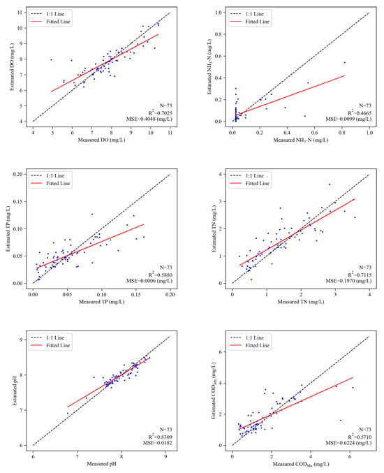
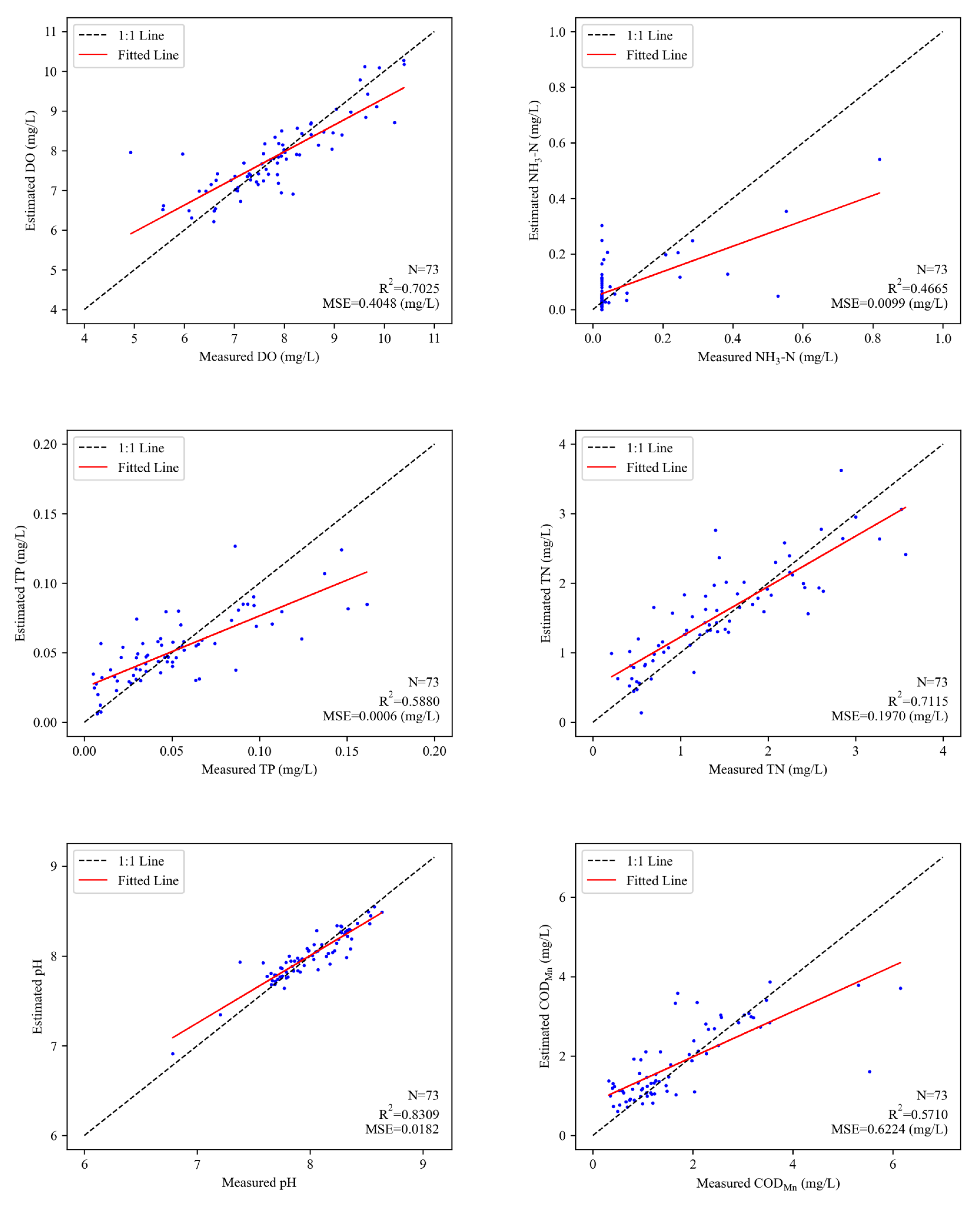
The fitted scatter plots obtained from the predictions of the best model for each water quality parameter on the validation dataset are presented in Figure 2. The prediction models for DO, TN, and pH demonstrated strong predictive performance, with R2 values exceeding 0.7 on the test dataset. Specifically, the DO model achieved an R2 of 0.7025 with an MSE of 0.4048 mg/L, the TN model reached an R2 of 0.7115 with an MSE of 0.1970 mg/L, and the pH model yielded an R2 of 0.8309 with an MSE of 0.0182. Although the best model for TP exhibited a relatively modest R2 of 0.5880, its MSE was only 0.0006 mg/L, indicating that the model still had considerable explanatory power for TP. For CODMn, the best prediction model achieved an R2 of 0.5710 and an MSE of 0.6224 mg/L on the test dataset. The NH3-N model performed less favorably compared to the other water quality parameters, but its R2 exceeded 0.4, indicating that the model retained a moderate level of predictive ability. An analysis of the fitted scatter plot for NH3-N revealed that a large proportion of observations were concentrated at 0.025 mg/L, suggesting a potential detection limit in NH3-N. From a modeling perspective, such value clustering reduces the effective variability of the water quality parameter and weakens the statistical relationship between input variables and NH3-N. This limited signal-to-noise ratio constrains the learning ability of data-driven models and leads to degraded predictive performance. The poor performance of the NH3-N model is not solely attributable to monitoring accuracy, but also reflects inherent methodological limitations in capturing low-variability. In the future, the accuracy of the model can be improved by using other models or by adding variables that may affect NH3-N. Overall, while all the prediction models tended to overestimate low values and underestimate high values, the model fits were generally satisfactory, demonstrating their potential applicability in river water quality monitoring.
Figure 2.
The fitting scatter plots of best models for water quality parameters.
3.4. Application of the Water Quality Parameters Prediction Model
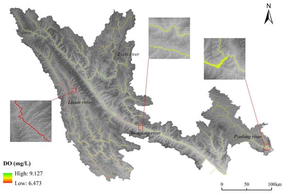
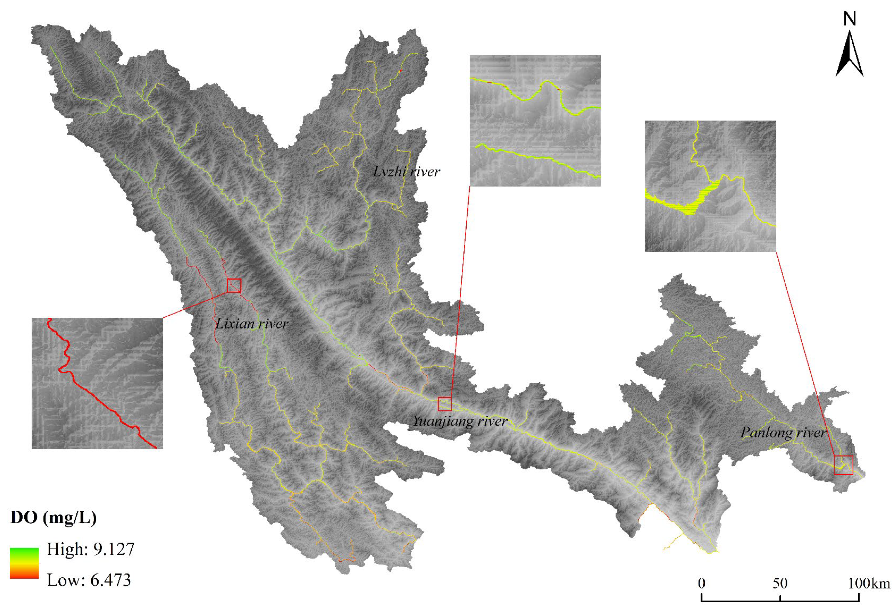
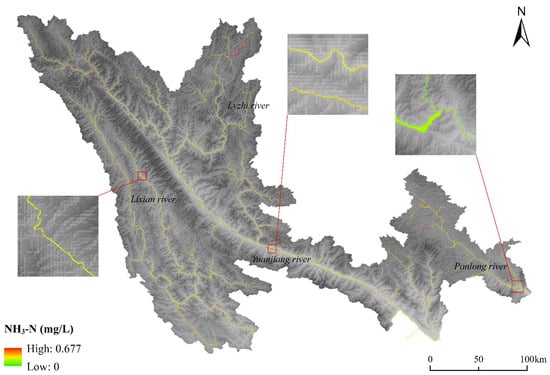
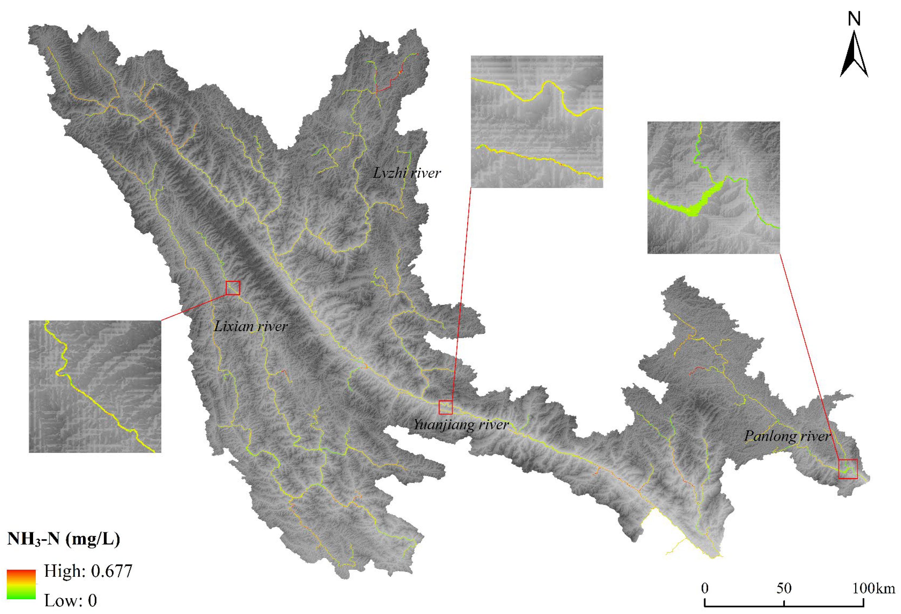
This study applied the optimized prediction models of six key water quality parameters across the entire RRB, demonstrating the innovative integration of machine learning with remote sensing for large-scale water quality monitoring. The water bodies were extracted using Google Earth Engine (GEE), leveraging its powerful cloud computing platform to process all Sentinel-2 images from 2023 with less than 10% cloud cover in the RRB. This approach ensured the acquisition of high-quality remote sensing data for subsequent water quality inversion. The inversion results for each water quality parameter are presented in Figure 3, Figure 4, Figure 5, Figure 6, Figure 7 and Figure 8.
Figure 3.
Inversion results of DO concentration in the RRB in 2023.
Figure 4.
Inversion results of NH3-N concentration in the RRB in 2023.
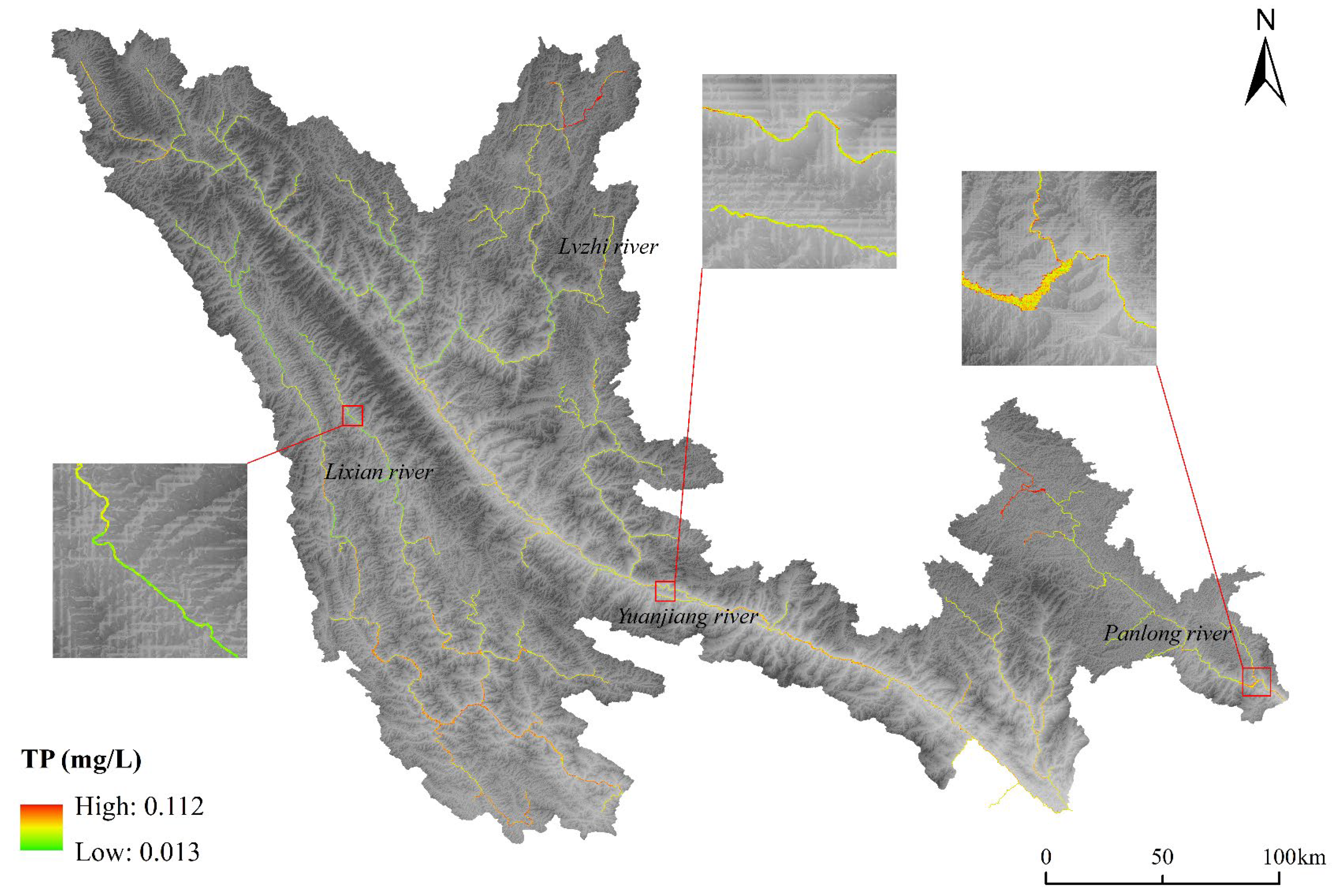
Figure 5.
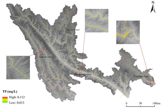
Inversion results of TP concentration in the RRB in 2023.
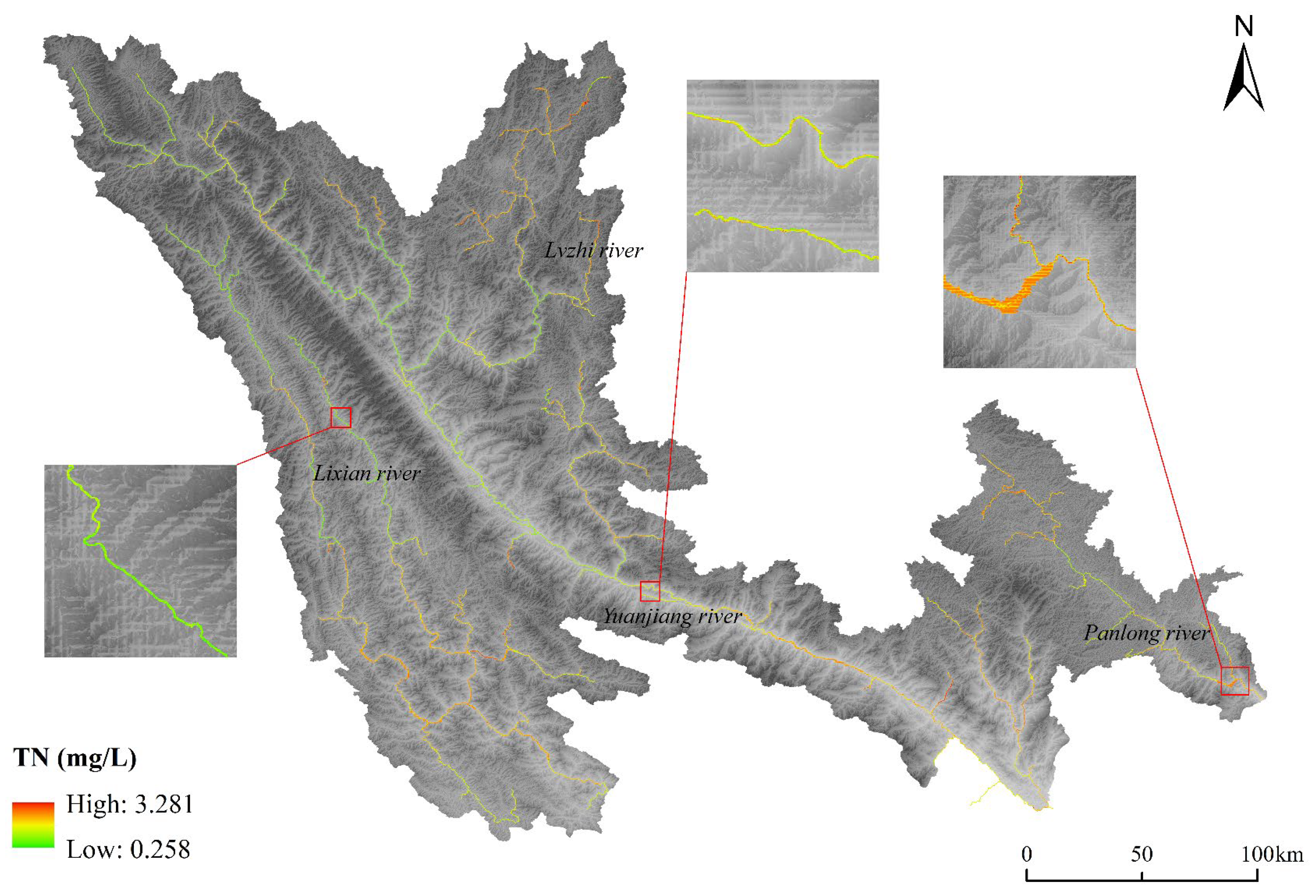
Figure 6.
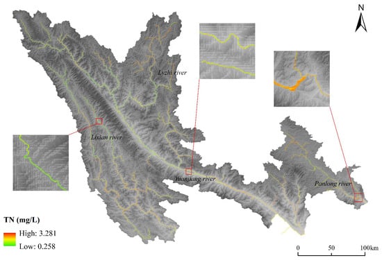
Inversion results of TN concentration in the RRB in 2023.
Figure 7.
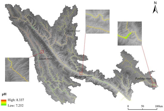
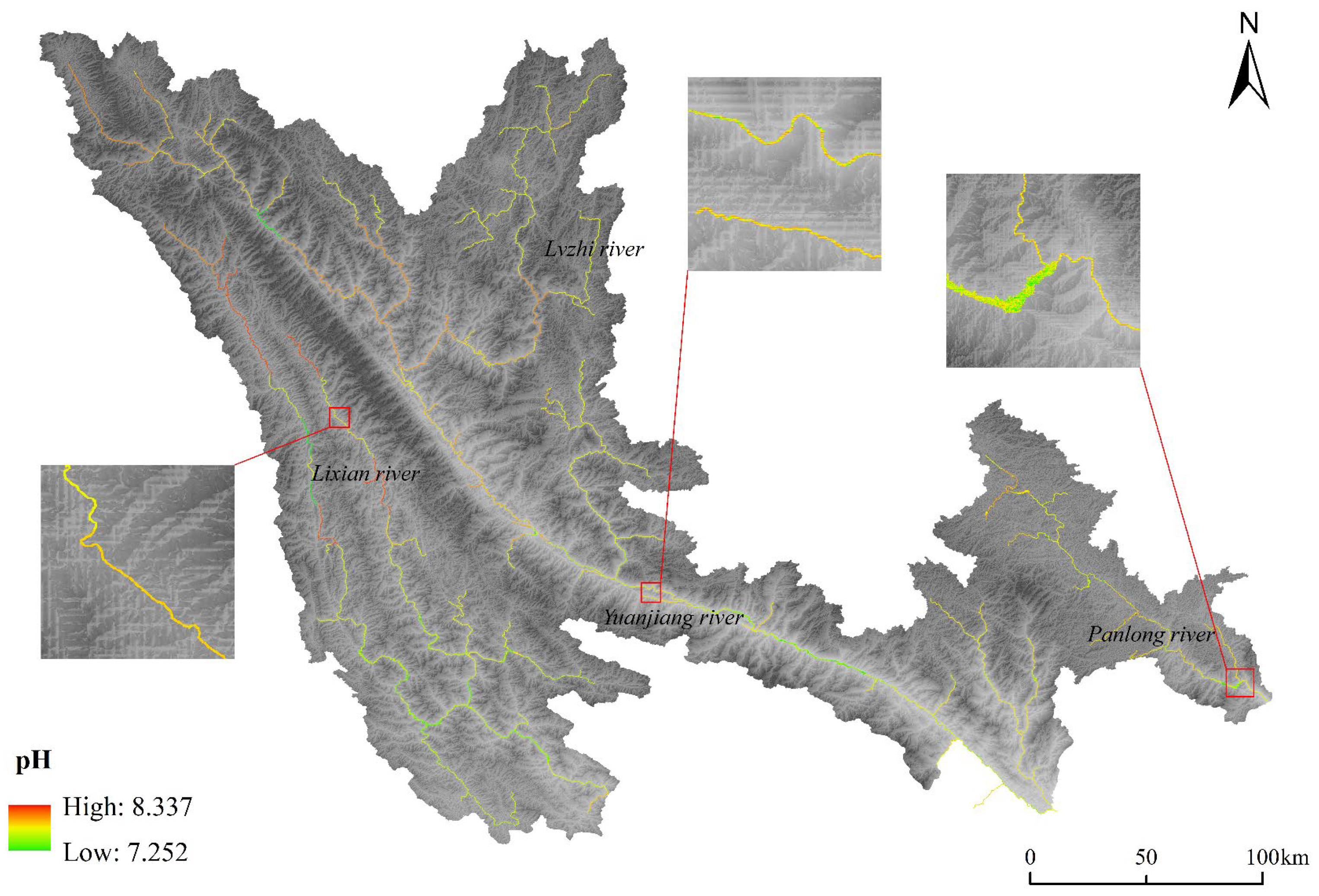
Inversion results of pH concentration in the RRB in 2023.
Figure 8.
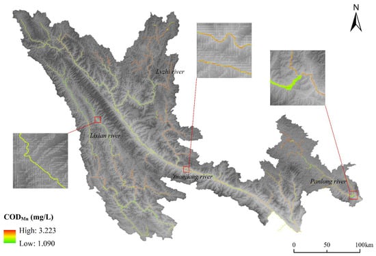
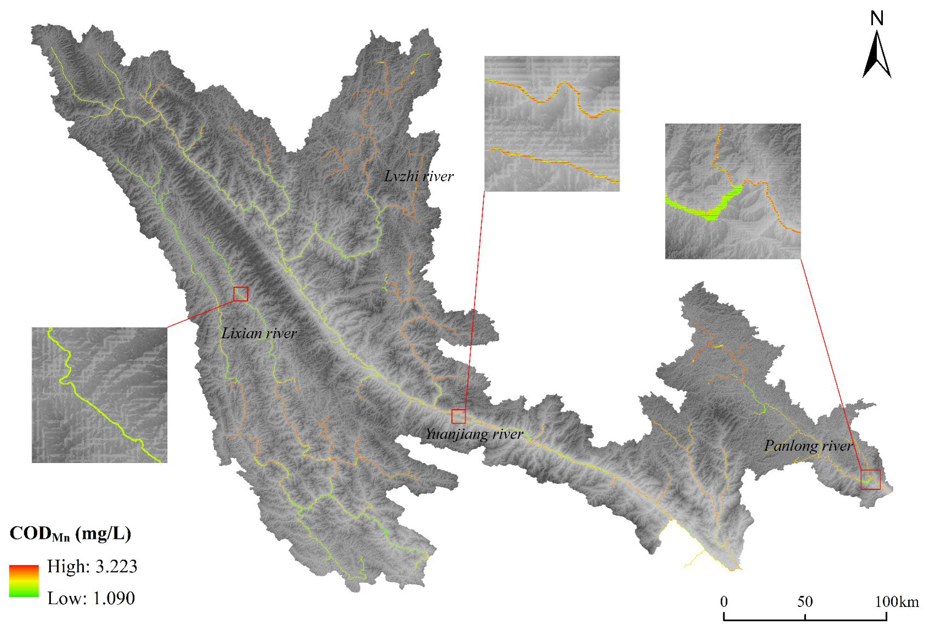
Inversion results of CODMn concentration in the RRB in 2023.
Figure 3 shows the distribution of DO concentrations, ranging from 6.473 to 9.127 mg/L. According to the Environmental Quality Standards for Surface Water (GB 3838-2002), all DO values in the basin meet at least Class II standards. Although DO levels in the midstream were slightly lower, they remained satisfactory overall. For NH3-N (Figure 4), the model predicted a maximum concentration of 0.677 mg/L, placing it within Class III water quality. The downstream regions showed higher NH3-N concentrations than upstream areas, likely due to more intensive human activities leading to nitrogen pollution [48]. The spatial distribution of TP (0.013–0.112 mg/L) in Figure 5 closely mirrors that of NH3-N, with significantly lower concentrations in the upstream areas compared to the middle and lower reaches. Overall, TP levels across the basin meet acceptable standards. Figure 6 displays TN concentrations, which ranged from 0.258 to 3.281 mg/L. Notably, the lowest TN concentrations still did not meet Class I standards, and concentrations in most middle and lower reaches exceeded 1.5 mg/L (Class IV–V standards), indicating serious nitrogen pollution. This finding underscores the need for improved regional production and living management and for effective control of urban nitrogen discharge to mitigate nitrogen pollution in the watershed. The inversion results for pH (Figure 7) ranged from 7.252 to 8.337, indicating that all values were within a suitable range without excessive acidity or alkalinity. CODMn concentrations (Figure 8) varied from 1.090 to 3.223 mg/L, meeting at least the Class II standard. High CODMn concentrations were mainly concentrated downstream, with additional hotspots in the Lvzhi River and the upper reaches of the Panlong River, suggesting potential natural sources of concern.
This study demonstrates the methodological advantages of integrating machine learning models optimized by WOA with multi-source data and GEE-based feature extraction. The results indicate that the proposed framework effectively captures spatial variability in water quality indicators, thereby validating the model’s capability to learn complex spatial patterns from heterogeneous environmental data. The proposed framework can effectively capture the spatial variation characteristics of water quality parameters, verifying the model’s ability to learn spatial patterns from different environmental data. The application of the model throughout the Red River Basin indicates that the design of this method is scalable and transferable, and is applicable to other river basins with similar data availability. The application of this method within the basin a new idea for regional water resource management and pollution control.
4. Discussion
4.1. SHAP Analysis of the Interpretability of Variables
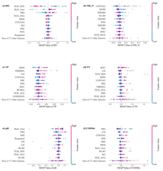
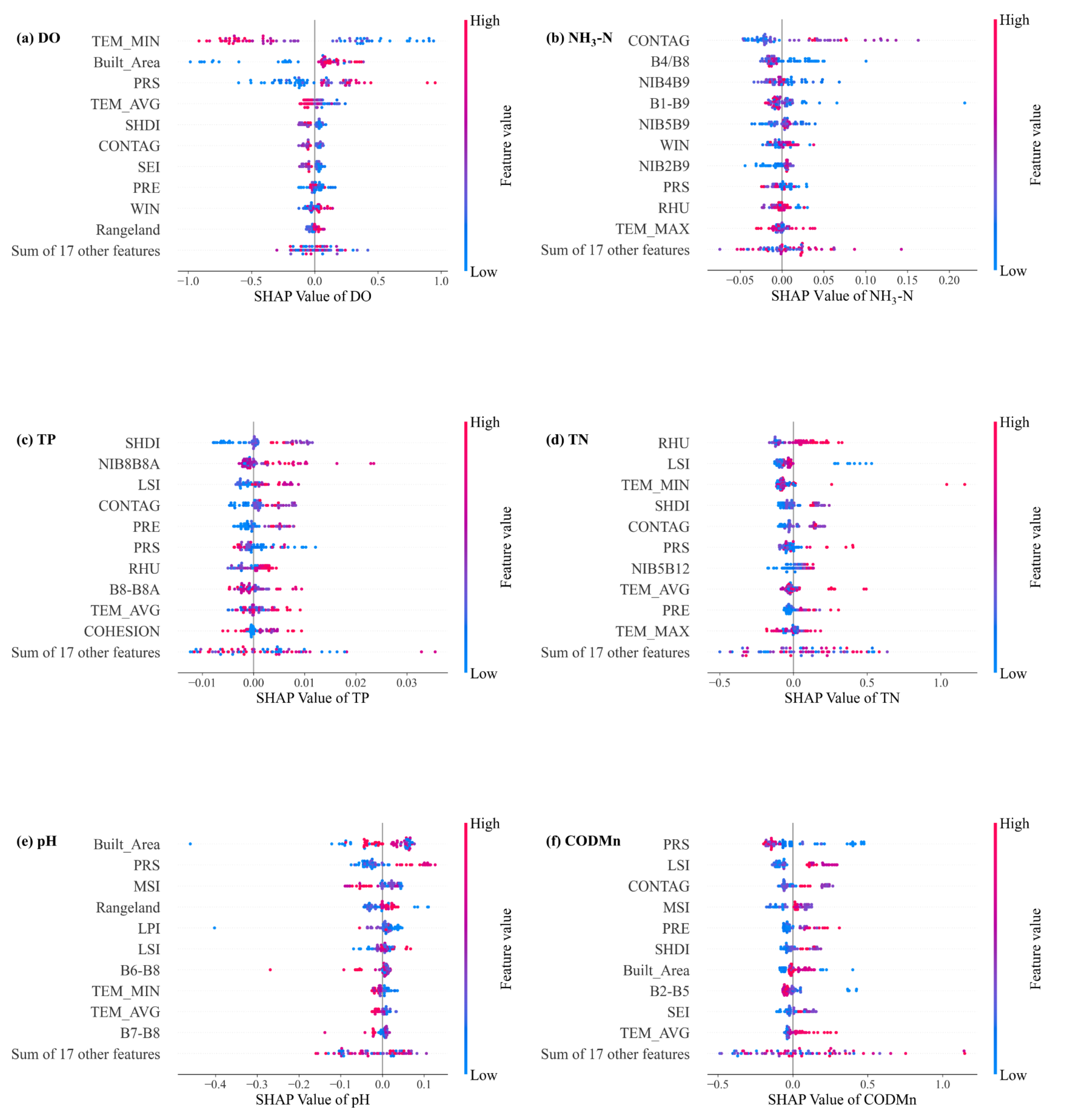
Due to the inherent lack of interpretability in many machine learning models, this study employs the SHAP model to analyze the importance of input variables for each water quality parameter. Figure 9 presents the global variable importance map generated by SHAP for each water quality parameter. For each sub-figure, the variables are ranked from top to bottom according to their decreasing importance. Each point in the figure represents a sample: red indicates higher variable values, while blue indicates lower variable values. The horizontal axis displays the SHAP value for each variable, reflecting its influence on the model’s output. Points to the left of the central axis indicate a negative contribution to the predicted value, while those to the right indicate a positive contribution.
Figure 9.
Global interpretability of SHAP for water quality parameters.
The results show that remote sensing imagery, meteorological data, land use, and landscape pattern indices all impact water quality parameters, although the specific sensitivities vary among them. For DO, meteorological variables such as TEM_MIN and PRS play a substantial role, with lower minimum temperatures corresponding to higher SHAP values (indicating a stronger positive effect on DO). The proportion of built-up area also shows a significant impact, suggesting that DO is sensitive to human activities within the basin. For NH3-N, SHAP reveals a strong dependence on remote sensing bands (B4/B8, NIB4B9, B1–B9). Notably, the CONTAG ranks highest in importance, highlighting the influence of water body aggregation and dispersion on NH3-N concentrations. TP and CODMn are both strongly influenced by landscape pattern indices, indicating that the spatial distribution of water bodies within the basin interacts closely with phosphorus and nitrogen dynamics. Specifically, SHDI, LSI, and CONTAG have prominent effects on TP, while the band combination NIB8B8A also contributes. It reflects the effects of land-use heterogeneity, landscape fragmentation, and spatial aggregation on phosphorus transport and retention processes. Higher SHDI and lower CONTAG usually imply a more heterogeneous and fragmented landscape, which enhances surface runoff pathways and soil erosion, thereby promoting particulate phosphorus transport into water bodies. CODMn is most affected by LSI, CONTAG, and MSI, with atmospheric pressure also playing a significant role. Complex landscape shapes (high LSI and MSI) increase the contact area between land and water bodies, facilitating the input and transformation of organic matter and consequently elevating CODMn. For TN, SHAP interpretability results suggest that both landscape pattern indices (LSI, SHDI) and meteorological variables (RHU, TEM_MIN) jointly influence the model’s output. Finally, pH is influenced by all categories of input variables, demonstrating the diversity and complexity of variables affecting pH. These findings underscore the complexity of river water quality parameters, indicating that remote sensing imagery alone is insufficient to fully explain water quality variability.
An overall inspection of Figure 9 reveals that while the importance of specific variables varies by water quality parameter, certain variables consistently exhibit significant influence, such as CONTAG, Built_Area, and TEM_MIN. This suggests that although different water quality parameters are driven by different sets of variables, there are also important interconnections among them. Interestingly, Built_Area impacts both DO and pH but in opposite directions, further illustrating the nuanced influence of input variables on water quality. Overall, the SHAP interpretability model provides valuable insights into both the direction and magnitude of variable influences, greatly aiding the analysis of water quality dynamics and supporting informed water quality management.
4.2. Impacts of Multiple Variables on Water Quality Prediction
Most prediction models for water quality parameters have historically relied solely on remote sensing data, while few studies have integrated meteorological and land use variables. In this study, the integration of multi-source data substantially improved the model’s ability to explain the observed spatial and temporal variability of water quality parameters, particularly for non-optically active parameters. The results suggest that meteorological, land use, and landscape patterns can affect water quality parameters by altering the generation, transmission, and accumulation of pollutants. Based on the SHAP interpretability analysis of water quality parameters, we discuss the influence path of input variables with large SHAP values on water quality.
Key meteorological elements—temperature, precipitation, and humidity—affect water quality both directly and indirectly. Environmental temperature can alter the physical properties and biological activities of water bodies. An increase in water temperature reduces the solubility of oxygen and accelerates the growth of algae. This not only reduces the DO concentration but also has an impact on TN (algae activities are often accompanied by the process of absorbing and releasing inorganic nitrogen). Precipitation has a significant impact on DO, pH and CODMn. More precipitation increases the total volume of surface runoff, allowing more organic matter to enter water bodies through surface runoff and causing the concentration of CODMn to rise. At the same time, the increase in water volume will dilute the original water body and accelerate the flow rate of the river, indirectly affecting the DO concentration and pH value. High humidity will increase the concentration of TN in water bodies. This might be an indirect transmission path: when the humidity is high, the moisture content of soil will increase, causing the residual nitrogen elements in the farmland to flow into water bodies, which leads to an increase in TN concentration.
Built-up areas near water bodies have an impact on river water quality. Built-up areas are hubs of human activity, where treated or untreated domestic sewage and industrial wastewater often enter the environment. Improper wastewater management can severely degrade water quality. Additionally, the expansion of impervious surfaces in built-up areas alters surface runoff patterns, leading to increased non-point source pollution.
Among the landscape pattern indices, CONTAG, SHDI and LSI have the greatest impact on water quality parameters. CONTAG indicates the degree of aggregation and connectivity of similar landscape. Given that the Red River Basin is dominated by the primary industry, high CONTAG might be due to contiguous farmland. This leads to the spatial concentration of fertilizer application, thereby increasing the concentration of NH3-N in water bodies. SHDI describes the diversity of landscape types, which has the greatest impact on TP. High SHDI indicates that the landscape types in the area are more diverse, resulting in a more varied source of TP in the water body. LSI represents the complexity of the landscape boundary. It has an impact on three water quality parameters (TP, TN and CODMn) for measuring pollutants. This might be because the boundary areas are more prone to human disturbance and natural erosion. The expansion of the boundary will increase soil erosion and contact area between farmland and water bodies, allowing phosphorus and organic matter to enter water bodies. The influence of LSI on TN is indirect. LSI may affect TN concentration by altering surface runoff. The above analysis is consistent with the SHAP values of LSI. LSI shows a significantly positive correlation with TP and CODMn, while it seems to have a nonlinear relationship with TN.
Based on the above analysis, it can be found that the machine learning model based on multi-source data proposed in this study can well explain the variables that affect water quality parameters. It provides a new analytical direction for the future management of water resources in river basins.
4.3. Potential of the Model Application in Broader Regions
Most previous studies have focused on urban rivers or lakes with relatively small spatial scales and stable water quality, while few have addressed large-scale watersheds. On the one hand, it is impractical to use UAVs or other equipment for large-scale water quality inversion; on the other hand, significant variations in water quality within large watersheds pose challenges for model construction. In this study, the model was developed using data from monitoring stations located in different segments of the RRB, enabling its application to the entire watershed. The model performance results indicate that it effectively predicts water quality parameters and is well-suited for diverse water bodies. Applying prediction models to fast-flowing and spatially extensive rivers—particularly across entire watersheds—remains a significant challenge. This study represents a valuable exploration of large-scale water quality inversion, offering technical support and a methodological framework for future research.
5. Conclusions
This study presents an innovative and interpretable modeling framework for large-scale river water quality inversion by integrating multi-source environmental data and heuristic-optimized machine learning techniques. Targeting six key water quality parameters (DO, NH3-N, TP, TN, pH, and CODMn), the proposed framework incorporates remote sensing imagery, meteorological variables, land use classification, and landscape pattern indices as input variables. A core methodological contribution lies in the use of the WOA to fine-tune hyperparameters of tree-based machine learning models (XGBoost and LightGBM), significantly enhancing model performance and generalization. In addition, the application of SHAP enables transparent interpretation of variable contributions, addressing the black-box nature of most machine learning approaches.
The optimized models achieved high predictive accuracy, with R2 values of 0.70 for DO, 0.46 for NH3-N, 0.59 for TP, 0.71 for TN, 0.83 for pH, and 0.57 for CODMn, confirming their effectiveness across diverse water quality parameters. Notably, the integration of landscape metrics and meteorological elements proved crucial in improving the inversion of non-optically active water quality parameters—an area traditionally limited by the reliance on remote sensing reflectance alone. Furthermore, the framework was successfully applied at the scale of the entire RRB (~61,700 km2), demonstrating its scalability, robustness, and practical feasibility in large, heterogeneous river systems. The spatial prediction maps generated using 2023 satellite imagery provide fine-scale, continuous estimates of water quality that can support basin-wide environmental decision-making and pollution control strategies. In conclusion, this study offers both methodological innovation and practical utility. By coupling multi-source data fusion with heuristic-optimized, interpretable machine learning models, it advances the capabilities of remote sensing-based water quality monitoring. The framework is transferable to other basins and provides a valuable decision-support tool for hydrological management, especially in regions facing data scarcity or complex watershed dynamics.
Supplementary Materials
The following supporting information can be downloaded at: https://www.mdpi.com/article/10.3390/rs18020320/s1, Table S1: The selected spectral bands or their combinations for the inversion of each water quality parameter.; Table S2: The hyperparameters of XGBoost and LightGBM optimized by the WOA.
Author Contributions
Conceptualization, Z.L. and F.W.; methodology, Z.L. and K.F.; formal analysis, Z.L. and K.F.; investigation, X.G.; data curation, K.F.; writing—original draft preparation, K.F.; writing—review and editing, Z.L., F.W. and X.G.; supervision, Z.L., F.W. and X.G.; funding acquisition, X.G. All authors have read and agreed to the published version of the manuscript.
Funding
This work was supported by the National Natural Science Foundation of China [Grant no. U2102208] and Major Project of the National Social Science Fund of China (Grant No. 23&ZD104).
Data Availability Statement
The data presented in this study are available upon request from the corresponding author.
Conflicts of Interest
The authors declare no conflict of interest.
Abbreviations
The following abbreviations are used in this manuscript:
| RF | Random Forest |
| XGBoost | eXtreme Gradient Boosting |
| LightGBM | Light Gradient Boosting Machine |
| WOA | Whale Optimization Algorithm |
| SHAP | Shapley Additive Explanations |
| RRB | Red River Basin |
| DO | dissolved oxygen |
| CODMn | chemical oxygen demand |
| TP | total phosphorus |
| TN | total nitrogen |
| NH3-N | ammonia nitrogen |
References
- Guo, J.; Bian, R.; Guan, A.; Cao, X.; Peng, J.; Wu, X.; Wang, D.; Qi, W.; Liu, H.; Qu, J. Assessment and identification of primary factors controlling Yangtze River water quality. ACS EST Water 2023, 3, 1329–1340. [Google Scholar] [CrossRef] [Scilit]
- Yan, C.; Zhang, W.; Zhang, Z.; Liu, Y.; Deng, C.; Nie, N. Assessment of water quality and identification of polluted risky regions based on field observations & GIS in the Honghe River Watershed, China. PLoS ONE 2015, 10, e0119130. [Google Scholar]
- Feng, Z.; Zhang, Z.; Zuo, Y.; Wan, X.; Wang, L.; Chen, H.; Xiong, G.; Liu, Y.; Tang, Q.; Liang, T. Analysis of long term water quality variations driven by multiple factors in a typical basin of Beijing-Tianjin-Hebei region combined with neural networks. J. Clean. Prod. 2023, 382, 135367. [Google Scholar] [CrossRef] [Scilit]
- Ge, Y.; Wu, Z.; Chen, Y.; Guo, P.; Wu, A.; Liu, H.; Yuan, G.; Li, Y.; Fu, H.; Jeppesen, E. Cascading effects of human activities and ENSO on the water quality of Poyang Lake in China. Catena 2024, 246, 108380. [Google Scholar] [CrossRef] [Scilit]
- Ren, X.; Yang, C.; Zhao, B.; Xiao, J.; Gao, D.; Zhang, H. Water quality assessment and pollution source apportionment using multivariate statistical and PMF receptor modeling techniques in a sub-watershed of the upper Yangtze River, Southwest China. Environ. Geochem. Health 2023, 45, 6869–6887. [Google Scholar] [CrossRef] [Scilit]
- Bangira, T.; Matongera, T.N.; Mabhaudhi, T.; Mutanga, O. Remote sensing-based water quality monitoring in African reservoirs, potential and limitations of sensors and algorithms: A systematic review. Phys. Chem. Earth Parts A/B/C 2024, 134, 103536. [Google Scholar] [CrossRef] [Scilit]
- Kouadri, S.; Elbeltagi, A.; Islam, A.R.M.T.; Kateb, S. Performance of machine learning methods in predicting water quality index based on irregular data set: Application on Illizi region (Algerian southeast). Appl. Water Sci. 2021, 11, 190. [Google Scholar] [CrossRef] [Scilit]
- Wu, Z.; Lai, X.; Li, K. Water quality assessment of rivers in Lake Chaohu Basin (China) using water quality index. Ecol. Indic. 2021, 121, 107021. [Google Scholar] [CrossRef] [Scilit]
- Chen, P.; Li, W.; He, K. Impacts of different types of El Niño events on water quality over the Corn Belt, United States. Hydrol Earth Syst Sc. 2022, 26, 4875–4892. [Google Scholar] [CrossRef] [Scilit]
- Shahid, M.S.B.; Rifat, H.R.; Uddin, M.A.; Islam, M.M.; Mahmud, M.Z.; Sakib, M.K.H.; Roy, A. Hypertuning-based ensemble machine learning approach for real-time water quality monitoring and prediction. Appl. Sci. 2024, 14, 8622. [Google Scholar] [CrossRef] [Scilit]
- Lai, Y.; Zhang, J.; Li, W.; Song, Y. Water quality monitoring of large reservoirs in China based on water color change from 1999 to 2021. J. Hydrol. 2024, 633, 130988. [Google Scholar] [CrossRef] [Scilit]
- Sun, X.; Zhang, Y.; Shi, K.; Zhang, Y.; Li, N.; Wang, W.; Huang, X.; Qin, B. Monitoring water quality using proximal remote sensing technology. Sci. Total Environ. 2022, 803, 149805. [Google Scholar] [CrossRef] [Scilit] [PubMed]
- Chen, J.; Wang, K.; Li, X.; Zhao, X.; Cheng, X.; Liu, Z.; Zhang, J.; Zhang, S. Remote sensing inversion of water quality parameters (TSM, Chl-a, and CDOM) in subtidal seaweed beds and surrounding waters. Ecol. Indic. 2024, 167, 112716. [Google Scholar] [CrossRef] [Scilit]
- Cao, Q.; Yu, G.; Qiao, Z. Application and recent progress of inland water monitoring using remote sensing techniques. Environ. Monit. Assess. 2023, 195, 125. [Google Scholar] [CrossRef] [Scilit] [PubMed]
- Chen, J.; Chen, S.; Fu, R.; Wang, C.; Li, D.; Peng, Y.; Wang, L.; Jiang, H.; Zheng, Q. Remote sensing estimation of chlorophyll-A in case-II waters of coastal areas: Three-band model versus genetic algorithm–artificial neural networks model. IEEE J. Sel. Topics Appl. Earth Observ. Remote Sens. 2021, 14, 3640–3658. [Google Scholar] [CrossRef] [Scilit]
- Thopanaiah, C.K.; CN, G.B.; Gurani, V.; Rajani, T.; Pavani, A.; Muthukumaran, D.; Deivasigamani, S. Advanced Remote Sensing and Generative Models for Comprehensive Water Quality Management in a Changing Climate. Remote Sens. Earth Syst. Sci. 2024, 7, 596–611. [Google Scholar] [CrossRef] [Scilit]
- Jiang, Y.; Kong, J.; Zhong, Y.; Zhang, J.; Zheng, Z.; Wang, L.; Liu, D. The optimal method for water quality parameters retrieval of urban river based on machine learning algorithms using remote sensing images. Int. J. Remote Sens. 2024, 45, 7297–7317. [Google Scholar] [CrossRef] [Scilit]
- Song, W.; Yinglan, A.; Wang, Y.; Fang, Q.; Tang, R. Study on remote sensing inversion and temporal-spatial variation of Hulun lake water quality based on machine learning. J. Contam. Hydrol. 2024, 260, 104282. [Google Scholar] [CrossRef] [Scilit]
- Tian, D.; Zhao, X.; Gao, L.; Liang, Z.; Yang, Z.; Zhang, P.; Wu, Q.; Ren, K.; Li, R.; Yang, C. Estimation of water quality variables based on machine learning model and cluster analysis-based empirical model using multi-source remote sensing data in inland reservoirs, South China. Environ. Pollut. 2024, 342, 123104. [Google Scholar] [CrossRef] [Scilit]
- Zhang, Y.; Li, W.; Wen, W.; Zhuang, F.; Yu, T.; Zhang, L.; Zhuang, Y. Universal high-frequency monitoring methods of river water quality in China based on machine learning. Sci. Total Environ. 2024, 947, 174641. [Google Scholar] [CrossRef] [Scilit]
- Harkort, L.; Duan, Z. Estimation of dissolved organic carbon from inland waters at a large scale using satellite data and machine learning methods. Water Res. 2023, 229, 119478. [Google Scholar] [CrossRef] [Scilit] [PubMed]
- Liang, Y.; Ding, F.; Liu, L.; Yin, F.; Hao, M.; Kang, T.; Zhao, C.; Wang, Z.; Jiang, D. Monitoring water quality parameters in urban rivers using multi-source data and machine learning approach. J. Hydrol. 2025, 648, 132394. [Google Scholar] [CrossRef] [Scilit]
- Bullard, J.E.; Ockelford, A.; O’Brien, P.; Neuman, C.M. Preferential transport of microplastics by wind. Atmos. Environ. 2021, 245, 118038. [Google Scholar] [CrossRef] [Scilit]
- Tiyasha, T.; Tung, T.M.; Bhagat, S.K.; Tan, M.L.; Jawad, A.H.; Mohtar, W.H.M.W.; Yaseen, Z.M. Functionalization of remote sensing and on-site data for simulating surface water dissolved oxygen: Development of hybrid tree-based artificial intelligence models. Mar. Pollut. Bull. 2021, 170, 112639. [Google Scholar] [CrossRef] [Scilit]
- Murphy, S.F.; Runkel, R.L.; Stets, E.G.; Nolan, A.J.; Repert, D.A. Urbanization and water management control stream water quality along a mountain to plains transition. Water Resour. Res. 2024, 60, e2023WR035633. [Google Scholar] [CrossRef] [Scilit]
- Wei, W.; Gao, Y.; Huang, J.; Gao, J. Exploring the effect of basin land degradation on lake and reservoir water quality in China. J. Clean. Prod. 2020, 268, 122249. [Google Scholar] [CrossRef] [Scilit]
- Xu, J.; Bai, Y.; You, H.; Wang, X.; Ma, Z.; Zhang, H. Water quality assessment and the influence of landscape metrics at multiple scales in Poyang Lake basin. Ecol. Indic. 2022, 141, 109096. [Google Scholar] [CrossRef] [Scilit]
- Shen, Z.; Hou, X.; Li, W.; Aini, G. Relating landscape characteristics to non-point source pollution in a typical urbanized watershed in the municipality of Beijing. Landsc. Urban Plan. 2014, 123, 96–107. [Google Scholar] [CrossRef] [Scilit]
- Tanaka, T.; Sato, T.; Watanabe, K.; Wang, Y.; Yang, D.; Inoue, H.; Li, K.; Inamura, T. Irrigation system and land use effect on surface water quality in river, at lake Dianchi, Yunnan, China. J. Environ. Sci. 2013, 25, 1107–1116. [Google Scholar] [CrossRef] [Scilit]
- Wang, J.; Yin, W.; Wang, L.; Li, N.; Hao, R.; Xu, J.; Xiao, H.; Zhong, Z.; Zhang, Y.; Shi, Z. Unraveling the effects of hydrological connectivity and landscape characteristics on reservoir water quality. J. Hydrol. 2022, 613, 128410. [Google Scholar] [CrossRef] [Scilit]
- Chen, J.; Fan, Y.; Zhang, Y.; Peng, J.; Zhang, J.; Cao, C. Comprehensive propagation characteristics between paired meteorological and hydrological drought events: Insights from various underlying surfaces. Atmos. Res. 2024, 299, 107193. [Google Scholar] [CrossRef] [Scilit]
- Deng, C.; Liu, L.; Li, H.; Peng, D.; Wu, Y.; Xia, H.; Zhang, Z.; Zhu, Q. A data-driven framework for spatiotemporal characteristics, complexity dynamics, and environmental risk evaluation of river water quality. Sci. Total Environ. 2021, 785, 147134. [Google Scholar] [CrossRef] [Scilit] [PubMed]
- GB 3838-2002; Environmental quality standard for surface water. Ministry of Ecology and Environment, PRC: Beijing, China, 2002.
- Wu, J.; Cheng, S.; He, L.; Wang, Y.; Yue, Y.; Zeng, H.; Xu, N. Assessing water quality in the Pearl River for the last decade based on clustering: Characteristic, evolution and policy implications. Water Res. 2023, 244, 120492. [Google Scholar] [CrossRef] [Scilit] [PubMed]
- Peng, K.; Si, B.; Jiang, W.; Ma, M.; Wang, X. Annual river dataset in China: A new product with a 10 m spatial resolution from 2016 to 2023. Earth Syst. Sci. Data Discuss 2024, 2024, 1–26. [Google Scholar]
- McGrane, S.J. Impacts of urbanisation on hydrological and water quality dynamics, and urban water management: A review. Hydrol. Sci. J. 2016, 61, 2295–2311. [Google Scholar] [CrossRef] [Scilit]
- Peng, S.; Li, S. Scale relationship between landscape pattern and water quality in different pollution source areas: A case study of the Fuxian Lake watershed, China. Ecol. Indic. 2021, 121, 107136. [Google Scholar] [CrossRef] [Scilit]
- Zhang, F.; Chen, Y.; Wang, W.; Jim, C.Y.; Zhang, Z.; Tan, M.L.; Liu, C.; Chan, N.W.; Wang, D.; Wang, Z. Impact of land-use/land-cover and landscape pattern on seasonal in-stream water quality in small watersheds. J. Clean. Prod. 2022, 357, 131907. [Google Scholar] [CrossRef] [Scilit]
- McGarigal, K. FRAGSTATS: Spatial Pattern Analysis Program for Quantifying Landscape Structure; US Department of Agriculture, Forest Service, Pacific Northwest Research Station: Portland, OR, USA, 1995.
- Teixidó, N.; Garrabou, J.; Arntz, W.E. Spatial pattern quantification of Antarctic benthic communities using landscape indices. Mar. Ecol. Prog. Ser. 2002, 242, 1–14. [Google Scholar] [CrossRef] [Scilit]
- Mirjalili, S.; Lewis, A. The whale optimization algorithm. Adv. Eng. Software 2016, 95, 51–67. [Google Scholar] [CrossRef] [Scilit]
- Breiman, L. Random forests. Mach. Learn. 2001, 45, 5–32. [Google Scholar] [CrossRef] [Scilit]
- Chen, T.; Guestrin, C. Xgboost: A scalable tree boosting system. In Proceedings of the 22nd Acm Sigkdd International Conference on Knowledge Discovery and Data Mining, San Francisco, CA, USA, 13–17 August 2016; pp. 785–794. [Google Scholar]
- Ke, G.; Meng, Q.; Finley, T.; Wang, T.; Chen, W.; Ma, W.; Ye, Q.; Liu, T. Lightgbm: A Highly Efficient Gradient Boosting Decision Tree. NeurIPS 2017, 3149–3157. Available online: https://papers.nips.cc/paper_files/paper/2017/hash/6449f44a102fde848669bdd9eb6b76fa-Abstract.html (accessed on 14 January 2026).
- Lundberg, S.M.; Lee, S.I. A unified approach to interpreting model predictions. In Proceedings of the 31st International Conference on Neural Information Processing Systems, Long Beach, CA, USA, 4–9 December 2017; pp. 4765–4774. [Google Scholar]
- Wang, W.; Yang, P.; Xia, J.; Huang, H.; Li, J. Impact of land use on water quality in buffer zones at different scales in the Poyang Lake, middle reaches of the Yangtze River basin. Sci. Total Environ. 2023, 896, 165161. [Google Scholar] [CrossRef] [Scilit]
- Xiao, R.; Wang, G.; Zhang, Q.; Zhang, Z. Multi-scale analysis of relationship between landscape pattern and urban river water quality in different seasons. Sci. Rep. 2016, 6, 25250. [Google Scholar] [CrossRef] [Scilit]
- Zhao, B.; Zhang, A.; Wang, H.; Pang, J.; Hou, Y.; Ma, P.; Zhao, B. Water function zone: A method to improve the accuracy of remote sensing retrieval of water bodies. Ecol. Indic. 2024, 164, 112105. [Google Scholar] [CrossRef] [Scilit]

Disclaimer/Publisher’s Note: The statements, opinions and data contained in all publications are solely those of the individual author(s) and contributor(s) and not of MDPI and/or the editor(s). MDPI and/or the editor(s) disclaim responsibility for any injury to people or property resulting from any ideas, methods, instructions or products referred to in the content. |
© 2026 by the authors. Licensee MDPI, Basel, Switzerland. This article is an open access article distributed under the terms and conditions of the Creative Commons Attribution (CC BY) license.