Proposed Methodology for Correcting Fourier-Transform Infrared Spectroscopy Field-of-View Scene-Change Artifacts

Highlights

What are the main findings?

• A theoretical basis was established for predicting the occurrence of scene-change artifacts in Fourier-transform spectroscopy.
• An easily implemented smooth offset correction (SOC) was developed to mitigate field-of-view scene-change artifacts, significantly reducing measurement error.

What is the implication of the main finding?

• The result reconciled the theoretical prediction of negligible scene-change artifacts with the experimental observations of significant scene-change artifacts.
• The SOC method enables accurate use of Fourier-transform spectroscopy when an object transitions through the field of view or when the field of view is changing.

Abstract

Fourier-transform spectrometers are widely used for spectral measurements. Changes in the field of view during measurement introduce oscillations into the measured spectra known as scene-change artifacts. Field-of-view changes also introduce uncertainty about which target the measured spectrum represents. Though scene-change artifacts are often present in dynamic data, their significance is disputed in the current literature. This work presents a theoretical framework and experimental validation for scene-change artifacts. Field-of-view changes introduce variable interferogram offsets, which standard processing techniques assume are constant. The error between the interferogram offset and its estimate is Fourier-transformed, yielding scene-change artifacts, often confused with noise, in the calibrated spectrum. Previous theoretical models ignored the effect of the interferogram offset in generating SCAs, leading to an underestimation of the scene-change artifact significance. Smooth offset correction removes these artifacts by estimating the variable interferogram offset using locally weighted scatter-plot smoothing. Updating the interferogram offset estimate resulted in the same accuracy expected for static conditions. The resulting spectra resemble the zero path difference spectra, similar to earlier theoretical predictions. These results indicate that Fourier-transform spectroscopy accuracy with variable scenes can be significantly improved with minor modifications to data processing.

1. Introduction

Determining the spectrum of a target is commonly accomplished using Fourier-transform spectrometers (FTSs) [1]. FTSs determine the incoming spectrum by Fourier-transforming the interferogram after subtracting the interferogram offset. The interferogram is typically obtained using a Michelson interferometer. FTSs offer several advantages over traditional dispersive spectrometers. FTSs offer higher speed, signal-to-noise, and spectral resolution [2]. Furthermore, FTSs offer greater versatility, as both the spectral resolution and collection speed can be adjusted to meet user needs without modifying any physical components [3]. Due to these advantages, FTSs have proliferated, especially in applications requiring rapid measurements, such as explosive events [4,5], turbulent engine exhaust [6], or industrial emissions [7,8]. However, changes within the FOV during measurement can alter the measured interferogram, introducing scene-change artifacts (SCAs) in the resulting spectra.

FTS processing techniques typically assume a static scene during measurement [9]. For instruments like the Telops Hyper-cam LW used in this study, data acquisition can take several seconds to over a minute [10]. Scene variability affects the observed spectrum in a more complex way than a simple time-average over the scan [11]. Kick addressed the uncertainty about which target is represented in the measured spectra, stating, “The real part of the spectrum we obtain is just the spectrum the FTS was seeing at the time when it was at the zero-path difference (ZPD) position” [12]. Kick developed this principle for a scenario in which a target entered the FOV right at the start of the interferogram scan. This work demonstrates that the same principle can be extended to more general FOV change scenarios. Kick’s theoretical analysis suggests that SCAs resulting from the scene changes are negligible in the real part of the spectrum. Subsequent simulation studies by Young and Gross agree with Kick’s predictions [13,14,15]. Later authors have used these theoretical predictions to discard potential SCAs in their observed spectra as noise [16,17]. However, experimental results from Mitchel and Manzardo contradict these theoretical predictions. They demonstrated instead that SCAs can significantly alter the measured spectra [18,19]. This discrepancy between Kick, Young, and Gross’s theoretical predictions and the experimental results of Mitchel and Manzardo can be explained by an additional source of SCAs. These additional SCAs are caused by incorrect interferogram offset removal.

Several prior efforts have addressed the removal of SCAs. The recombobulate correction method (RCM) has proven effective in mitigating SCAs caused by oscillatory scene changes [20]. Statistical approaches have been shown to reduce SCAs arising from stochastic scene variability [21,22,23]. However, these methods require multiple interferograms to achieve effective correction.

This work focuses on a common scenario in which the target enters or exits the field of view (FOV) during measurement [24]. Previous theoretical development of SCAs ignored potential issues in interferogram offset removal. Traditional processing of the measured interferogram assumes a constant interferogram offset. This process yields noticeable SCAs on the real component of the spectrum that were not predicted by previous theory. A theoretical basis is presented demonstrating that these SCAs result from an incorrect interferogram offset estimate. This work demonstrates that accurate interferogram offset removal eliminates nearly all SCAs in the resulting spectrum. Unlike prior approaches, the method presented here corrects FOV SCAs using a single interferogram.

This paper describes the procedure for processing FTS data. The interferogram offset error propagates through the process, producing SCAs in the final spectrum. Next, this work describes simulating FOV SCAs and conducting equivalent experiments. Simulations depict SCA behavior under a variety of conditions. SCAs are greater for brighter targets, broader spectral range, better spectral resolution, lower wavenumbers, and have larger brightness differences between targets. The interferogram offset was estimated using a polynomial fit. This correction effectively removes SCAs from the calibrated spectrum. Smooth offset correction (SOC) was developed to accurately estimate the interferogram offset in experimental data. When applied to experimental data, SOC outperformed the polynomial fit. Processing experimental data with the SOC interferogram offset estimate effectively removed SCAs from the calibrated spectra. Correcting the interferogram offset estimation requires modifying the computational steps without altering experimental data collection. Thus, SCAs in FTS spectra caused by scene changes can be effectively removed through minor modifications to the data processing. Additionally, this correction can be applied retroactively to previously collected FTS data.

2. Materials and Methods

2.1. FTS and SCA Theory

We begin by examining how an interferogram is measured. An incoming target spectrum is incident on the interferometer. The interferometer splits the incoming beam and sends the separated beams along two paths of different lengths. Then, the beams are recombined at the detector. The difference in path length between the two beams is called the optical path difference (OPD). The OPD is controlled by varying one beam’s path length. The two beams interfere constructively or destructively depending on the OPD. For example, at zero path difference (ZPD), the beams interfere constructively [25]. Measuring the detector signal as the OPD varies produces the measured interferogram, given by the following:

$${\mathrm{I}}_{\mathrm{m}}(\mathrm{x})=\mathrm{a}(\mathrm{x})[\mathrm{I}(\mathrm{x})+{\mathrm{I}}_{\mathrm{o}}(\mathrm{x})],$$

(1)

where ${\mathrm{I}}_{\mathrm{m}}(\mathrm{x})$ is the measured interferogram, $\mathrm{a}(\mathrm{x})$ is the apodization function, $\mathrm{I}\left(\mathrm{x}\right)$ is the interferogram without offset, ${\mathrm{I}}_0(\mathrm{x})$ is the interferogram offset (also known as the DC component), and x is the OPD [26]. If no apodization is applied, a(x) is replaced by the truncation function, which defines the limits of the measured interferogram. Notably, the term “interferogram” is used inconsistently in the literature. It is used to refer to both ${\mathrm{I}}_{\mathrm{m}}(\mathrm{x})$ and $\mathrm{I}(\mathrm{x})$, depending on the source [27]. This inconsistency may have contributed to discrepancies between theoretical predictions and experimental results in the literature. Kick and Young’s theoretical analyses begin with $\mathrm{I}(\mathrm{x})$, the interferogram without offset, while Mitchell and Manzardo’s results are based on processing ${\mathrm{I}}_{\mathrm{m}}(\mathrm{x})$, the measured interferogram.

For scenes with a constant observed spectrum, the interferogram offset is also constant and can be estimated by averaging the measured interferogram [28]. Subtracting this estimate from the measured interferogram yields the interferogram without offset estimate, given by the following:

$${\mathrm{I}}_{\mathrm{est}}(\mathrm{x})={\mathrm{I}}_{\mathrm{m}}(\mathrm{x})-{\mathrm{I}}_{\mathrm{o},\mathrm{est}},$$

(2)

However, when the input spectrum varies, the interferogram offset estimate becomes inaccurate, leaving a residual term that introduces SCAs into the resulting spectra when processed. Substituting Equation (1) into Equation (2) and applying the Fourier transform yields the raw spectrum, given by the following:

$${\mathrm{L}}_{\mathrm{raw}}(\nu )=\mathfrak{I}\left\{\mathrm{a}(\mathrm{x})\left[\mathrm{I}(\mathrm{x})+{\mathrm{I}}_{\mathrm{o}}\left(\mathrm{x}\right)-{\mathrm{I}}_{\mathrm{o},\mathrm{est}}\right]\right\},$$

(3)

where ${\mathrm{L}}_{\mathrm{r}\mathrm{a}\mathrm{w}}(\nu )$ is the raw spectrum, and $\mathfrak{I}$ denotes the Fourier transform given by the following:

$$\mathfrak{I}\left[\mathrm{f}\left(\mathrm{x}\right)\right]={\int }_{-\mathrm{\infty }}^{\mathrm{\infty }}\mathrm{f}(\mathrm{x}){\mathrm{e}}^{-\mathrm{i}2\pi \nu \mathrm{x}}\mathrm{d}\mathrm{x}$$

(4)

where $\nu$ is the wavenumber [29]. For numerical data, the interferogram without offset is zero-filled and transformed using the fast Fourier transform (FFT) [30]. The truncation of the interferogram at the maximum optical path difference (MOPD) limits spectral resolution and introduces oscillations near sharp features in the spectrum. To decrease these oscillations, it is common to apply an apodization function to the interferogram. The apodization function approaches zero at MOPD, thus eliminating the discontinuity. This reduces oscillations in the spectra around sharp changes at the expense of worsening spectral resolution [31]. This work focuses on the truncation of the interferogram, and therefore, a(x) will be replaced by the rectangular (rect) function given by the following:

$$\mathrm{a}\left(\mathrm{x}\right)=\mathrm{r}\mathrm{e}\mathrm{c}\mathrm{t}\left({\displaystyle \frac{\mathrm{x}-{\mathrm{x}}_{\mathrm{c}}}{{\mathrm{x}}_{\mathrm{a}}}}\right)=\left\{\begin{array}{cc}1,& {\mathrm{x}}_{\mathrm{c}}-{\displaystyle \frac{{\mathrm{x}}_{\mathrm{a}}}{2}}\le \mathrm{x}\le {\mathrm{x}}_{\mathrm{c}}+{\displaystyle \frac{{\mathrm{x}}_{\mathrm{a}}}{2}}\\ 0,& \mathrm{e}\mathrm{l}\mathrm{s}\mathrm{e}\end{array}\right.$$

(5)

where ${\mathrm{x}}_{\mathrm{c}}$ is the center of the interferogram, and ${\mathrm{x}}_{\mathrm{a}}$ is the full width of the apodization function. For a double-sided interferogram, the center ${\mathrm{x}}_{\mathrm{c}}$ is near ZPD, and the interferogram width ${\mathrm{x}}_{\mathrm{a}}$ is approximately twice the MOPD. For a single-sided interferogram, the center is near half of the MOPD, and the interferogram width is close to the MOPD.

The raw spectrum is measured in detector-specific units, such as volts or counts, and must be calibrated before it can be compared to the target spectrum. The raw spectrum is calibrated using the following:

$${\mathrm{L}}_{\mathrm{t},\mathrm{cal}}(\nu )={\displaystyle \frac{{\mathrm{L}}_{\mathrm{t},\mathrm{r}\mathrm{a}\mathrm{w},}(\nu )}{{\mathrm{G}}_{\mathrm{e}\mathrm{s}\mathrm{t}}(\nu )}}-{\mathrm{O}}_{\mathrm{e}\mathrm{s}\mathrm{t}}(\nu )$$

(6)

where ${\mathrm{L}}_{\mathrm{t},\mathrm{r}\mathrm{a}\mathrm{w}}(\nu )$ is the target’s raw spectrum, ${\mathrm{G}}_{\mathrm{e}\mathrm{s}\mathrm{t}}(\nu )$ is the estimated calibration gain, and ${\mathrm{O}}_{\mathrm{e}\mathrm{s}\mathrm{t}}(\nu )$ is the estimated calibration offset. Estimating the calibration gain and offset requires two additional raw spectra from known sources. These are typically obtained from a hot and cold blackbody source. The raw spectra from these blackbodies are used to estimate calibration gain and offset, using the following:

$${\mathrm{G}}_{\mathrm{e}\mathrm{s}\mathrm{t}}\left(\nu \right)={\displaystyle \frac{{\mathrm{L}}_{\mathrm{h}\mathrm{o}\mathrm{t},\mathrm{r}\mathrm{a}\mathrm{w}}\left(\nu \right)-{\mathrm{L}}_{\mathrm{c}\mathrm{o}\mathrm{l}\mathrm{d},\mathrm{r}\mathrm{a}\mathrm{w}}\left(\nu \right)}{{\mathrm{L}}_{\mathrm{h}\mathrm{o}\mathrm{t}}\left(\nu \right)-{\mathrm{L}}_{\mathrm{c}\mathrm{o}\mathrm{l}\mathrm{d}}\left(\nu \right)}}$$

(7)

and

$${\mathrm{O}}_{\mathrm{e}\mathrm{s}\mathrm{t}}\left(\nu \right)={\displaystyle \frac{{\mathrm{L}}_{\mathrm{c}\mathrm{o}\mathrm{l}\mathrm{d},\mathrm{r}\mathrm{a}\mathrm{w}}\left(\nu \right){\mathrm{L}}_{\mathrm{h}\mathrm{o}\mathrm{t}}\left(\nu \right)-{\mathrm{L}}_{\mathrm{h}\mathrm{o}\mathrm{t},\mathrm{r}\mathrm{a}\mathrm{w}}(\nu ){\mathrm{L}}_{\mathrm{c}\mathrm{o}\mathrm{l}\mathrm{d}}\left(\nu \right)}{{\mathrm{L}}_{\mathrm{h}\mathrm{o}\mathrm{t},\mathrm{r}\mathrm{a}\mathrm{w}}\left(\nu \right)-{\mathrm{L}}_{\mathrm{c}\mathrm{o}\mathrm{l}\mathrm{d},\mathrm{r}\mathrm{a}\mathrm{w}}(\nu )}},$$

(8)

where ${\mathrm{L}}_{\mathrm{h}\mathrm{o}\mathrm{t},\mathrm{r}\mathrm{a}\mathrm{w}}\left(\nu \right)$ and ${\mathrm{L}}_{\mathrm{c}\mathrm{o}\mathrm{l}\mathrm{d},\mathrm{r}\mathrm{a}\mathrm{w}}\left(\nu \right)$ are the raw spectra of the hot and cold blackbody sources, respectively, and ${\mathrm{L}}_{\mathrm{h}\mathrm{o}\mathrm{t}}\left(\nu \right)$ and ${\mathrm{L}}_{\mathrm{c}\mathrm{o}\mathrm{l}\mathrm{d}}\left(\nu \right)$ are their corresponding known spectra [32,33]. The calibration offset depends on the detector characteristics and is distinct from the interferogram offset, which depends on the incoming spectrum. The calibrated spectrum obtained from Equation (6) provides an estimate of the target’s true spectrum. The estimated spectrum, raw spectra, calibration gain, and calibration offset are each complex variables; however, the imaginary component of the estimated spectrum is discarded, and only the real components are examined in this work.

SCAs observed in the calibrated spectrum originate from the inaccuracies in the interferogram offset estimate used in Equation (3). The SCAs in the raw spectrum arise from taking the Fourier transform of the interferogram offset estimation error:

$${\mathrm{L}}_{\mathrm{raw},\mathrm{SCA}}(\nu )= \mathfrak{I}\left\{\mathrm{a}(\mathrm{x})\left[{\mathrm{I}}_{\mathrm{o}}\left(\mathrm{x}\right)-{\mathrm{I}}_{\mathrm{o},\mathrm{est}}\right]\right\} ,$$

(9)

The SCAs in the calibrated spectrum are obtained by dividing the raw spectrum SCAs by the estimated gain. These artifacts can be corrected by improving the estimation of the interferogram offset. Rather than using an average to estimate a constant interferogram offset, this approach fits a smooth function to the measured interferogram to determine the variable interferogram offset. Once the interferogram offset is accurately estimated and subtracted, the associated SCAs in the resulting spectrum are eliminated.

SCAs will be simulated under a variety of conditions to demonstrate their appearance in the calibrated spectrum, identify factors that influence their severity, and evaluate the effectiveness of the correction. The impact of SCAs and the effectiveness of the correction will then be validated through experimental measurements.

2.2. FTS FOV Simulation

Before the experiments, simulations were performed to observe the expected dependencies. For the simulations, measured spectra were built from truth spectra by working backwards through the measurement process to create simulated measured interferograms. The simulation assumed a cold blackbody and a hot blackbody, with their spectra defined by the Planck blackbody radiation law:

$$\mathrm{L}\left(\nu ,\mathrm{T}\right)=\mathsf{ϵ}2\mathrm{h}{\mathrm{c}}^2{\nu }^3{\displaystyle \frac{1}{{\mathrm{e}}^{\frac{\mathrm{h}\mathrm{c}\nu }{\mathrm{k}\mathrm{T}}}-1}},$$

(10)

where $\mathsf{ϵ}$ is the emissivity set to 1, h is Planck’s constant, c is the speed of light, k is Boltzmann’s constant, and T is the temperature in kelvin [34]. Unless otherwise specified, the truth spectrum was simulated with 1 cm⁻¹ resolution. The FTS detector response was simulated by applying a calibration gain and offset to the truth spectrum, yielding the uncalibrated spectrum given by the following:

$${\mathrm{L}}_{\mathrm{uncal}}(\nu )=\mathrm{G}\left(\nu \right)\left[\mathrm{L}(\nu )+\mathrm{O}\left(\nu \right)\right]$$

(11)

where $\mathrm{G}(\nu )$ is the calibration gain, $\mathrm{L}(\nu )$ is the incoming spectrum, and $\mathrm{O}(\nu )$ is the calibration offset [35]. While the uncalibrated spectrum is similar to the raw spectrum, it does not include apodization effects, which are present in the raw spectrum.

The uncalibrated spectrum is then turned into a simulated interferogram without offset by reflecting the spectrum across the y-axis and then taking the inverse Fourier transform [36]. The interferogram without offset, $\mathrm{I}(\mathrm{x})$, in Equation (1) is given by the following:

$$\mathrm{I}(\mathrm{x})= {{\displaystyle \frac{1}{2}}\mathfrak{I}}^{-1}\left[{\mathrm{L}}_{\mathrm{uncal}}(\nu )+{\mathrm{L}}_{\mathrm{uncal}}(-\nu )\right],$$

(12)

where ${\mathfrak{I}}^{-1}$ is the inverse Fourier transform given by the following:

$${\mathfrak{I}}^{-1}\left[\mathrm{F}\left(\nu \right)\right]={\int }_{-\mathrm{\infty }}^{\mathrm{\infty }}\mathrm{F}(\nu ){\mathrm{e}}^{\mathrm{i}2\pi \nu \mathrm{x}}\mathrm{d}\nu .$$

(13)

Although in practice, the inverse Fourier transform is computed using an inverse fast Fourier transform (IFFT). The interferogram offset, ${\mathrm{I}}_{\mathrm{o}}$ in Equation (1), can be determined using Equation (12):

$${\mathrm{I}}_0=\mathrm{I}(0),$$

(14)

which corresponds to the value of the interferogram without offset at ZPD [37]. It is important to note that for a constant target spectrum, the interferogram offset remains constant. Adding together the interferogram without offset and the interferogram offset gives the measured interferogram for the target spectrum. This process is outlined in Figure 1.

Figure 1. Flow chart for simulating a measured interferogram. The blackbody spectrum has the calibration gain and offset applied to generate the uncalibrated spectrum. Applying an IFFT to the uncalibrated spectrum produces the interferogram without offset. The interferogram offset is then added, producing a simulated measured interferogram.

Repeating the process for the second target produces the simulated measured interferogram for the second target. A scene function, $\mathrm{s}(\mathrm{x})$, is then applied to the measured interferograms of both targets. The scene function represents the fraction of the FOV filled by the targets, varying between zero and one. Applying the scene function to the targets’ measured interferogram and summing the result yields the measured interferogram of the combined simulated scene given by the following:

$${\mathrm{I}}_{\mathrm{m}}(\mathrm{x})=\mathrm{a}(\mathrm{x})\left\{ {[1-\mathrm{s}\left(\mathrm{x}\right)]\mathrm{I}}_{1,\mathrm{m}}\left(\mathrm{x}\right)+\mathrm{s}\left(\mathrm{x}\right){\mathrm{I}}_{2,\mathrm{m}}(\mathrm{x})\right\},$$

(15)

where ${\mathrm{I}}_{1,\mathrm{m}}\left(\mathrm{x}\right)$ and ${\mathrm{I}}_{2,\mathrm{m}}\left(\mathrm{x}\right)$ are the measured interferograms of the simulated targets. Substituting Equation (1) into Equation (15) yields the following:

$${\mathrm{I}}_{\mathrm{m}}(\mathrm{x})= \mathrm{a}(\mathrm{x})\left\{[1-\mathrm{s}\left(\mathrm{x}\right)]{[\mathrm{I}}_1\left(\mathrm{x}\right)+{\mathrm{I}}_{1,\mathrm{o}}]+\mathrm{s}\left(\mathrm{x}\right)[{\mathrm{I}}_2\left(\mathrm{x}\right)+{\mathrm{I}}_{2,\mathrm{o}}]\right\}.$$

(16)

Separating the interferogram offsets and subtracting the estimated interferogram offsets yields the following:

$${\mathrm{I}}_{\mathrm{m}}(\mathrm{x})= \mathrm{a}(\mathrm{x})\left\{\left[1-\mathrm{s}\left(\mathrm{x}\right)\right]{\mathrm{I}}_1\left(\mathrm{x}\right)+\mathrm{s}\left(\mathrm{x}\right){\mathrm{I}}_2\left(\mathrm{x}\right)+\left[1-\mathrm{s}\left(\mathrm{x}\right)\right]{\mathrm{I}}_{1,\mathrm{o}}+\mathrm{s}\left(\mathrm{x}\right){\mathrm{I}}_{2,\mathrm{o}}-{\mathrm{I}}_{\mathrm{o},\mathrm{e}\mathrm{s}\mathrm{t}}\left(\mathrm{x}\right)\right\},$$

(17)

Applying a Fourier transform then yields the following:

$${\mathrm{L}}_{\mathrm{raw}}(\nu )= {\mathrm{L}}_{\mathrm{r}\mathrm{a}\mathrm{w},\mathrm{Z}\mathrm{P}\mathrm{D}}\left(\nu \right)+{\mathrm{L}}_{\mathrm{r}\mathrm{a}\mathrm{w},\mathrm{S}\mathrm{C}\mathrm{A}}\left(\nu \right),$$

(18)

where ${\mathrm{L}}_{\mathrm{r}\mathrm{a}\mathrm{w},\mathrm{Z}\mathrm{P}\mathrm{D}}\left(\nu \right)$ is the spectrum observed at ZPD, as derived by Kick [12]. ${\mathrm{L}}_{\mathrm{r}\mathrm{a}\mathrm{w},\mathrm{S}\mathrm{C}\mathrm{A}}\left(\nu \right)$ represents the SCAs in the spectrum caused by inaccurate offset estimation during the FOV transition. This expression is similar to Equation (9), except that the interferogram offset here is a weighted sum of the target interferogram offsets. The weighting is determined by the scene function. If the interferogram offset is accurately estimated, this term vanishes. However, performing in this way requires a variable, rather than constant, interferogram offset estimate.

To enable calibration, two additional blackbodies were simulated and the raw spectrum from Equation (18) was calibrated using Equation (6). The resulting calibrated spectrum is then compared to the spectrum at ZPD to calculate the normalized root mean square error (NRMSE) given by the following:

$$\mathrm{NRMSE}={\displaystyle \frac{1}{{\mathrm{n}}^2\{\max \left[{\mathrm{L}}_{\mathrm{ZPD}}(\nu )\right]-\min \left[{\mathrm{L}}_{\mathrm{ZPD}}(\nu )\right]\}}}\sqrt{\sum _{\mathrm{i}=1}^{\mathrm{n}}{\left\{\mathrm{R}\mathrm{e}[{\mathrm{L}}_{\mathrm{c}\mathrm{a}\mathrm{l}}({\nu }_{\mathrm{i}})]-{\mathrm{L}}_{\mathrm{ZPD}}\left({\nu }_{\mathrm{i}}\right)\right\}}^2},$$

(19)

where the range of the ZPD spectrum is given by $\mathrm{m}\mathrm{a}\mathrm{x}[{\mathrm{L}}_{\mathrm{Z}\mathrm{P}\mathrm{D}}(\nu )]-\mathrm{m}\mathrm{i}\mathrm{n}[{\mathrm{L}}_{\mathrm{Z}\mathrm{P}\mathrm{D}}(\nu )]$. Here, L(${\nu }_{\mathrm{i}}$) is the measured spectrum at wavenumber ${\nu }_{\mathrm{I}}$, ${\mathrm{L}}_{\mathrm{Z}\mathrm{P}\mathrm{D}}({\nu }_{\mathrm{i}})$ is the truth spectrum at ZPD and the ith wavenumber, and n is the total number of spectral points [38,39]. Only the real part of the spectrum is analyzed, and only within the wavenumber range covered by the simulated detector response.

For each simulated scenario, two interferogram offset estimation methods were used. The first used the standard method, which estimates the interferogram offset by averaging the measured interferogram. The second interferogram offset estimate was determined by fitting a smoothing function to the measured interferogram. Each interferogram offset estimate was subtracted from the measured interferogram and then processed to produce a calibrated spectrum. The NRMSE was then compared before and after applying the correction. Lastly, a static scene without SCAs was simulated as a control case. This control is an important comparison because apodization and Gibbs phenomena prevent the elimination of error, even in the absence of SCAs.

2.3. FOV Scene-Change Experiment

The FTS used was a Telops Hyper-cam LW (Telops, Quebec City, QC, Canada). It operates in the longwave infrared (LWIR) spectrum range from $861 {\mathrm{cm}}^{-1}$ to $1306 {\mathrm{cm}}^{-1}$. Spectral data was collected at $1 {\mathrm{cm}}^{-1}$ resolution with a 64 × 64 pixel grid, requiring 2 s per interferogram scan [40]. The FOV of the 64 × 64 grid is 1.28°. The OPD for each pixel is modified by a factor of cos$\mathsf{\theta },$ where $\mathsf{\theta }$ is the half angle from the optical axis to the pixel line of sight (chief ray). For our setup, this value was a maximum of 0.99987, corresponding to a 0.12 cm⁻¹ correction to the spectral axis. This is much smaller than the measured wavenumber values of 800–1350 cm⁻¹, and so it was neglected [41]. A 6-inch Fluke 4181 blackbody (Fluke, Everett, WA, USA), with an emissivity of 0.96, was positioned 3.67 m from the FTS and used for the calibration and transition. For calibration, the blackbody was set to 323 K (50 °C) and 473 K (200 °C). During FOV transitions tests, the blackbody was set to 423 K (150 °C) [42].

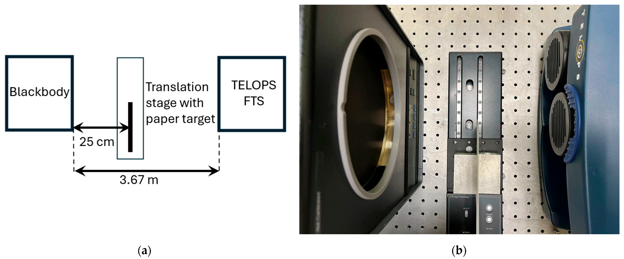
A flat paper, with emissivity between 0.90 and 0.98, was mounted on a ThorLabs LTS150 Long Travel Linear Stage (ThorLabs, Newton, NJ, USA) [43,44]. The stage was positioned between the blackbody and the FTS, 25 cm from the blackbody. The experimental setup is displayed in Figure 2. The experiment was conducted indoors on 07 August 2025 and completed in under two hours. Atmospheric transmission and path radiance were assumed to be constant and incorporated into the calibration gain and offset estimates [45]. The translation stage required 10 s to move the paper across the entire 8 cm, 64-pixel wide FOV, allowing several scans to be collected with different pixels affected by SCAs [46]. Additional scans were collected with the paper fully obscuring the blackbody and with the blackbody fully unobscured. While not required for SCA correction, these scans were used to determine the expected spectrum at ZPD.

Figure 2. Experimental setup. (a) A blackbody was observed by a Telops FTS hyperspectral imager at a distance of 3.67 m. Between the two, a paper target, positioned 25 cm away from the blackbody, was moved through the FOV. Diagram not to scale. (b) Photograph of the experimental setup. The equipment was temporarily moved closer together for the image.

Each interferogram was first processed using the standard offset estimation method and then reprocessed using the updated interferogram offset estimation. For each interferogram, the fraction of the FOV occupied by the paper and the blackbody at ZPD was estimated. These fractions, along with the fully obscured and unobscured spectra, were used to estimate the expected spectrum at ZPD. The calibrated spectrum, with and without correction, was compared to the expected ZPD spectrum to assess accuracy. This process was repeated for each pixel.

3. Results

3.1. FOV Transition Simulation Results

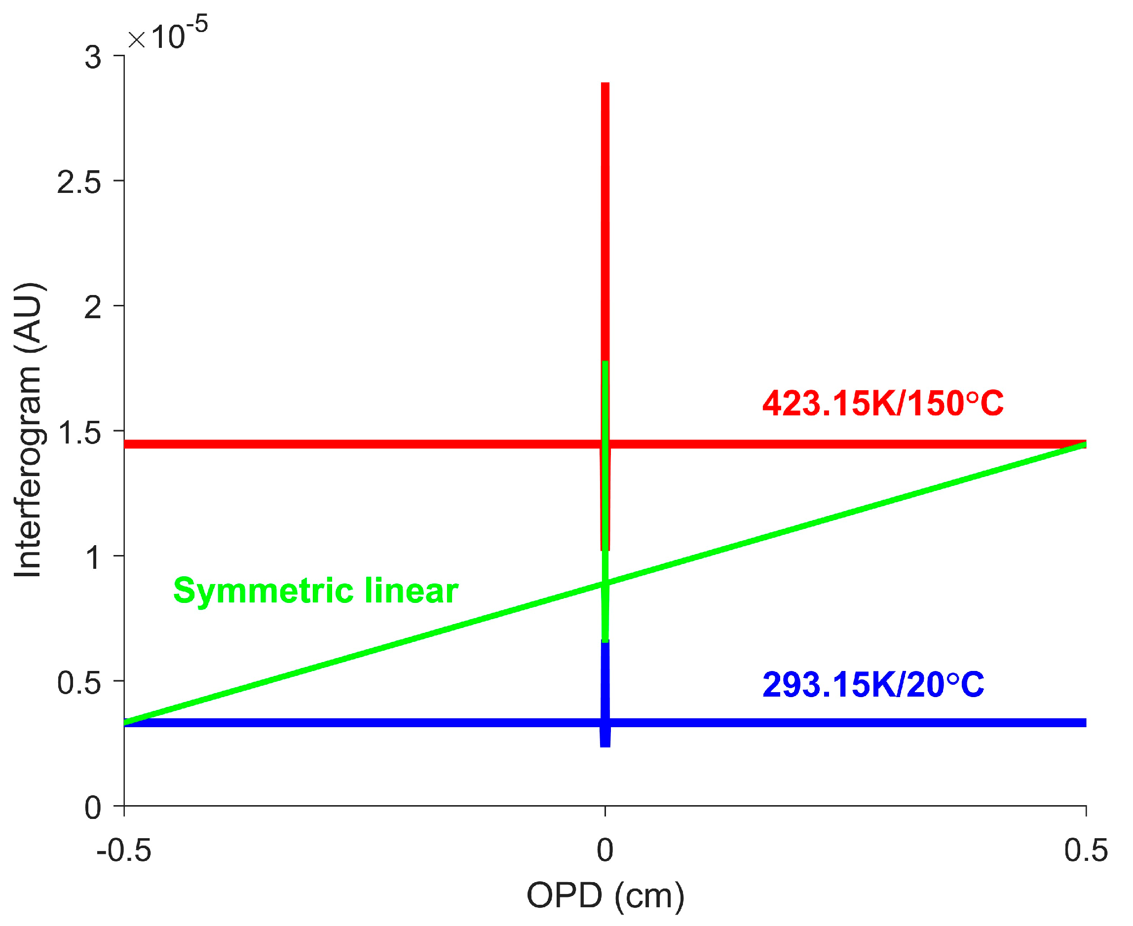
The first simulation models a hot blackbody entering the FOV at constant speed. At the initial OPD position, the FOV is completely filled by the cold, 293 K (20 °C) blackbody. At this point, the transitional measured interferogram matches the measured interferogram of the cold blackbody. At the final OPD position, the FOV is completely filled by the hot, 423 K (150 °C), blackbody. Here, the transitional measured interferogram matches the measured interferogram of the hot blackbody. This scenario is referred to as a linear symmetric FOV transition, represented by the scene function:

$$\mathrm{s}(\mathrm{x})={\displaystyle \frac{1}{2}}+{\displaystyle \frac{\mathrm{x}}{{\mathrm{x}}_{\mathrm{a}}}},$$

(20)

where ${\mathrm{x}}_{\mathrm{a}}$ is the full width of the apodization function, defined by the following:

$${\mathrm{x}}_{\mathrm{a}}= 2 {\mathrm{x}}_{\mathrm{M}\mathrm{O}\mathrm{P}\mathrm{D}}-\mathrm{d}\mathrm{x},$$

(21)

where ${\mathrm{x}}_{\mathrm{M}\mathrm{O}\mathrm{P}\mathrm{D}}$ is the MOPD and dx is the spacing between two interferogram positions. The scene function starts at zero at the beginning of the interferogram and linearly increases to one by the end. The apodization function, given in Equation (5), truncates the measured interferogram. Substituting the apodization and scene functions from Equations (5) and (20) into Equation (17) yields the following:

$${\mathrm{I}}_{\mathrm{m}}(\mathrm{x})= \mathrm{rect}({\displaystyle \frac{\mathrm{x}-{\mathrm{x}}_{\mathrm{c}}}{{\mathrm{x}}_{\mathrm{a}}}})\left\{\left[{\displaystyle \frac{1}{2}}-{\displaystyle \frac{\mathrm{x}}{{\mathrm{x}}_{\mathrm{a}}}}\right]{\mathrm{I}}_1\left(\mathrm{x}\right)+\left[{\displaystyle \frac{1}{2}}+{\displaystyle \frac{\mathrm{x}}{{\mathrm{x}}_{\mathrm{a}}}}\right]{\mathrm{I}}_2\left(\mathrm{x}\right)+\left[{\displaystyle \frac{1}{2}}-{\displaystyle \frac{\mathrm{x}}{{\mathrm{x}}_{\mathrm{a}}}}\right]{\mathrm{I}}_{1,\mathrm{o}}+\left[{\displaystyle \frac{1}{2}}+{\displaystyle \frac{\mathrm{x}}{{\mathrm{x}}_{\mathrm{a}}}}\right]{\mathrm{I}}_{2,\mathrm{o}}-{\mathrm{I}}_{\mathrm{o},\mathrm{e}\mathrm{s}\mathrm{t}}\left(\mathrm{x}\right)\right\}.$$

(22)

Figure 3 shows the measured interferogram for the simulated linear symmetric FOV transition.

Figure 3. Measured interferogram for the simulated linear symmetric FOV transition. The blue and red lines represent the interferograms for the 293 K (20 °C) blackbody and the 423 K (150 °C) blackbody, respectively. The green line shows the measured interferogram for the FOV transition. The non-constant interferogram offset is not accurately removed.

When the Fourier transform is applied to Equation (22), the first two terms in the curly brackets yield the raw spectrum at ZPD. In traditional processing, the interferogram offset is estimated as constant. This estimate is sufficient to eliminate the constant terms, with the third and fourth terms shown in red in Equation (22), but terms with a linear dependence on x will remain. Substituting the remainder into Equation (9) and factoring out the constants yields the following:

$${\mathrm{L}}_{\mathrm{r}\mathrm{a}\mathrm{w},\mathrm{S}\mathrm{C}\mathrm{A}}\left(\nu \right)= {\displaystyle \frac{{\mathrm{I}}_{2,\mathrm{o}}-{\mathrm{I}}_{1,\mathrm{o}}}{{\mathrm{x}}_{\mathrm{a}}}}\mathfrak{I}\left[\mathrm{rect}({\displaystyle \frac{\mathrm{x}-{\mathrm{x}}_{\mathrm{c}}}{{\mathrm{x}}_{\mathrm{a}}}})\mathrm{x}\right].$$

(23)

Applying the Fourier transform yields the SCAs, given by the following:

$$\begin{gathered} {\mathrm{L}}_{\mathrm{r}\mathrm{a}\mathrm{w},\mathrm{SCA}}(\nu )=({\mathrm{I}}_{2,\mathrm{o}}-{\mathrm{I}}_{1,\mathrm{o}})\{ \\ {\mathrm{x}}_{\mathrm{a}}{\mathrm{x}}_{\mathrm{c}}\mathrm{s}\mathrm{i}\mathrm{n}\mathrm{c}\left({\mathrm{x}}_{\mathrm{a}}\nu \right)\mathrm{s}\mathrm{i}\mathrm{n}\mathrm{c}\left(2{\mathrm{x}}_{\mathrm{c}}\nu \right)+{\mathrm{x}}_{\mathrm{a}}{\mathrm{x}}_{\mathrm{c}}\mathrm{s}\mathrm{i}\mathrm{n}\mathrm{c}\left({\mathrm{x}}_{\mathrm{a}}\nu \right)\cos \left(2\pi {\mathrm{x}}_{\mathrm{c}}\nu \right)-{\mathrm{x}}_{\mathrm{a}}{\mathrm{x}}_{\mathrm{c}}\cos \left(\pi {\mathrm{x}}_{\mathrm{a}}\nu \right)\mathrm{s}\mathrm{i}\mathrm{n}\mathrm{c}\left(2{\mathrm{x}}_{\mathrm{c}}\nu \right) \\ +\mathrm{i}2\pi \nu {\mathrm{x}}_{\mathrm{a}}{\mathrm{x}}_{\mathrm{c}}^2\mathrm{s}\mathrm{i}\mathrm{n}\mathrm{c}\left({\mathrm{x}}_{\mathrm{a}}\nu \right)\mathrm{s}\mathrm{i}\mathrm{n}\mathrm{c}\left(2{\mathrm{x}}_{\mathrm{c}}\nu \right)-{\displaystyle \frac{\mathrm{i}{\mathrm{x}}_{\mathrm{a}}}{2\pi \nu }}\mathrm{s}\mathrm{i}\mathrm{n}\mathrm{c}\left({\mathrm{x}}_{\mathrm{a}}\nu \right)\cos \left(2\pi {\mathrm{x}}_{\mathrm{c}}\nu \right)+{\displaystyle \frac{\mathrm{i}{\mathrm{x}}_{\mathrm{a}}}{2\pi \nu }}\cos \left(\pi {\mathrm{x}}_{\mathrm{a}}\nu \right)\cos \left(2\pi {\mathrm{x}}_{\mathrm{c}}\nu \right)\}. \end{gathered}$$

(24)

For a full derivation of Equation (24), see Appendix A. This analysis considers only the real part of the spectrum; the imaginary component of the SCAs is discarded. The SCAs contain four frequencies determined by the width and center of the interferogram. These SCAs can easily be mistaken for noise in the spectrum. The interferogram width is proportional to the MOPD, which is set by the desired spectral resolution. Improving spectral resolution increases MOPD, which also increases the magnitude of SCAs. The interferogram center is near zero for double-sided interferograms, but it significantly affects the appearance of SCAs when comparing SCAs from single-sided interferograms or double-sided interferograms.

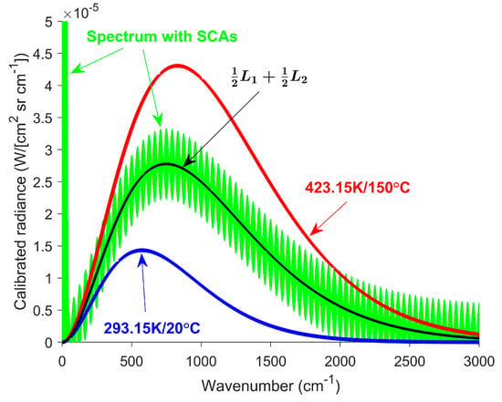
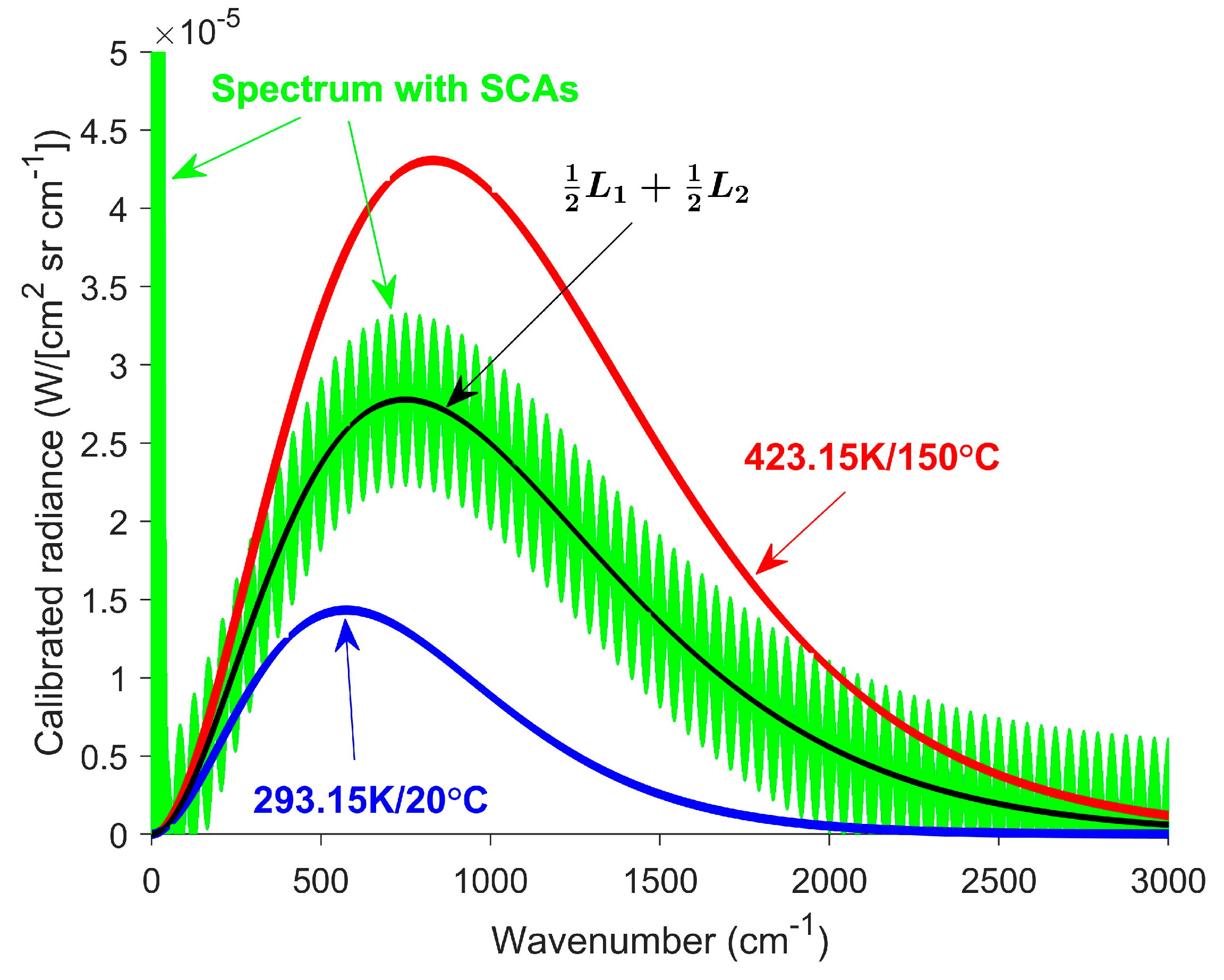
Additionally, a cold blackbody, 323 K (50 °C), and a hot blackbody, 473 K (200 °C), were simulated for calibration. When the green interferogram in Figure 3 is processed using the standard method, significant SCAs appear in the resulting spectrum, as shown in Figure 4.

Figure 4. Calibrated spectrum for the simulated linear symmetric FOV transition. The red and blue lines represent the spectra for the cold blackbody and hot blackbody, respectively. The green line is the calibrated spectrum obtained from processing the transition interferogram shown in Figure 3. The black line shows the spectrum at ZPD. The non-constant interferogram offset produces SCAs when it is removed by subtracting a constant offset estimate.

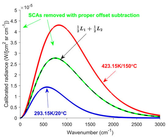
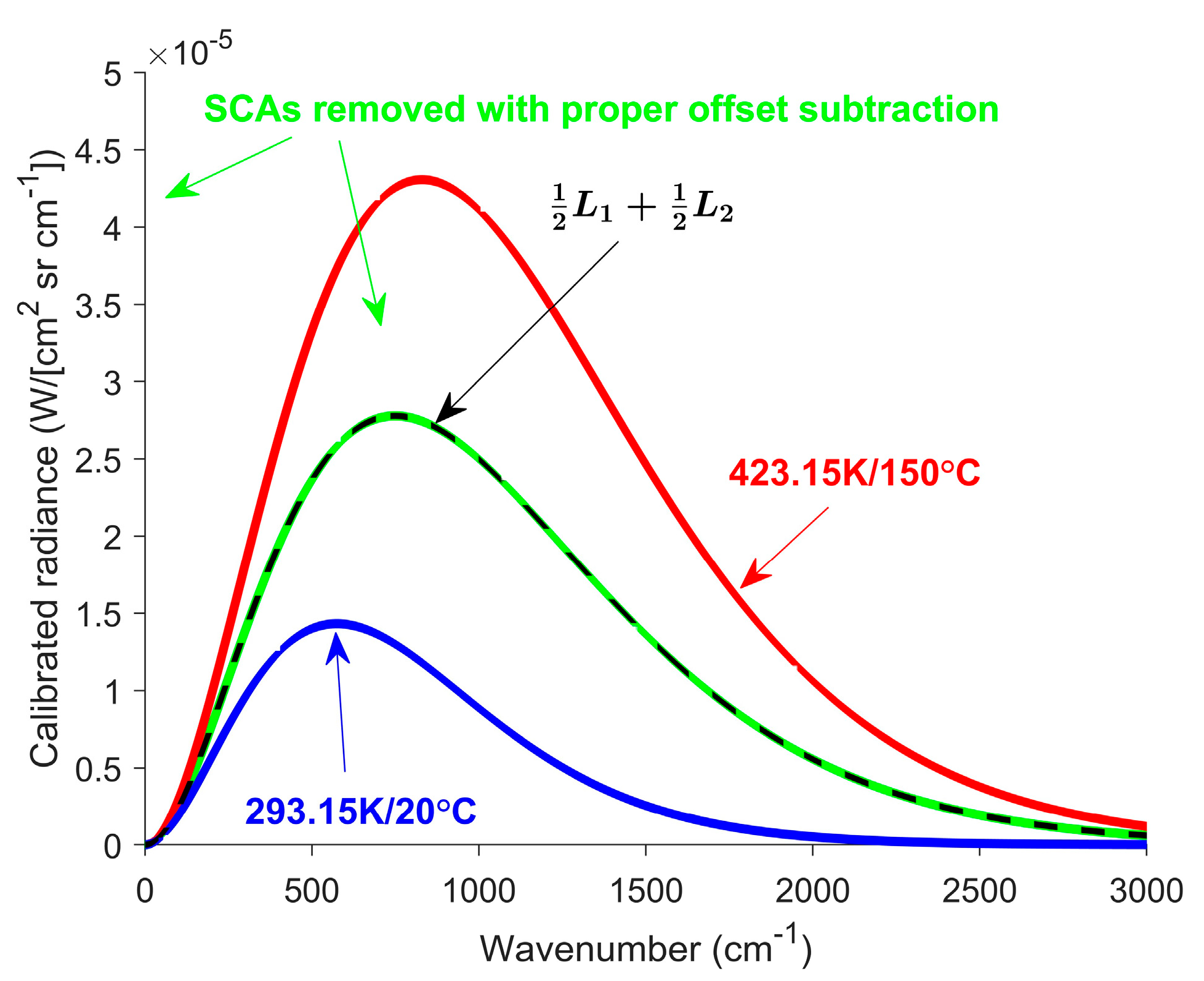
While the calibrated spectrum is centered on the ZPD spectrum, as predicted by Kick, it contains significant SCAs. A large peak near-zero wavenumber is expected due to the slow changes in interferogram offset shown in Figure 3. Additionally, the SCA oscillations slowly decrease in magnitude, leading to lower errors at higher wavenumbers. SCAs are also observed in the imaginary component of the spectrum. After complex calibration or phase correction, SCAs present in the imaginary component of the raw spectrum can affect the real component of the calibrated spectrum. Fortunately, accurate removal of the interferogram offset eliminates SCAs in both the real and imaginary components of the spectrum. Based on Equation (9) and Figure 3, replacing the constant interferogram offset with a linear fit provides a more accurate estimate and removes the SCAs described in Equations (24) and (25) and shown in Figure 5. With this correction, the corrected spectrum closely matches the ZPD spectrum.

Figure 5. Calibrated spectrum after correction for the simulated linear symmetric FOV transition. The red and blue lines represent the spectra for the cold blackbody and hot blackbody, respectively. The green line shows the calibrated spectrum after SCA correction. The black line represents the ZPD spectrum.

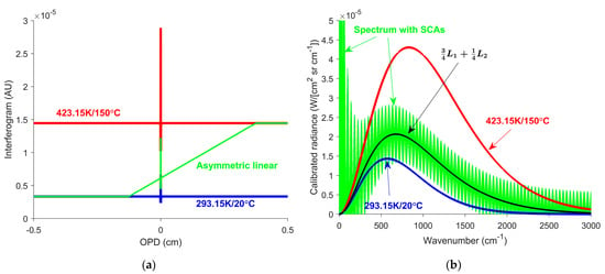
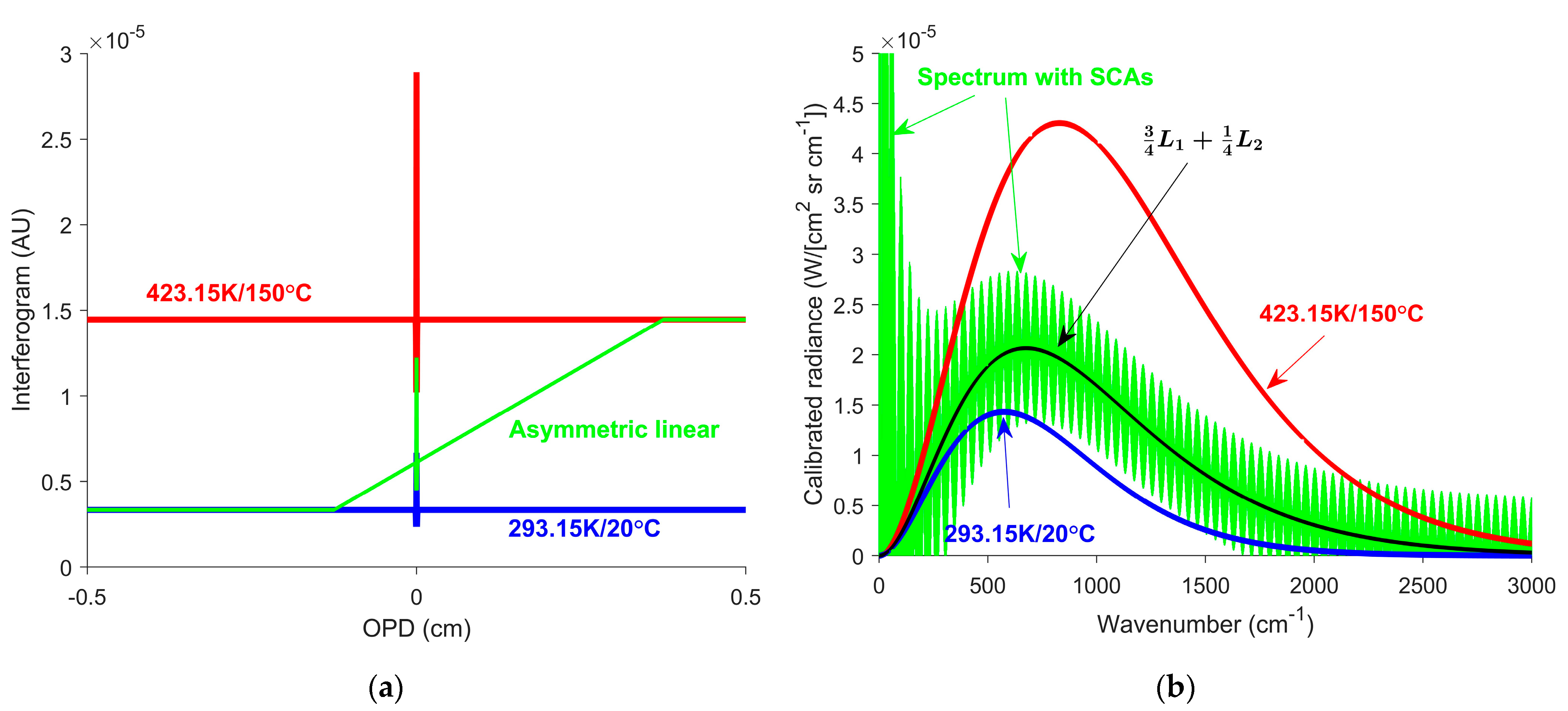
After correction, there is strong agreement between the ZPD spectrum (black) and the calibrated spectrum (green). However, in practice, it is unlikely that an object will begin and complete its transition exactly at the start and end of the interferogram. Instead, most transitions will be asymmetric, as illustrated in Figure 6a. In these cases, the calibrated spectrum remains centered around the ZPD spectrum, but the ZPD spectrum is no longer the average of the blackbodies. For FOV transitions, the ZPD spectrum is a weighted average of the blackbody spectra, based on their respective fractions of the FOV.

Figure 6. Measured interferogram and calibrated spectrum for simulated linear asymmetric FOV transition with SCAs. (a) The red and blue lines represent the measured interferograms for the 293 K (20 °C) cold blackbody and the 423K (150 °C) hot blackbody, respectively. The green line shows the measured interferogram as the hot blackbody transits the FOV. (b) The red and blue lines show the calibrated spectra of the hot and cold blackbodies, respectively. The green line is the calibrated spectrum resulting from processing the interferogram in (a). The black line represents the ZPD spectra.

The same correction process used for the symmetric case is applied to the asymmetric case, with minor modifications. In the symmetric case, a single linear fit is sufficient to estimate the interferogram offset across the entire interferogram. For the asymmetric case, an accurate interferogram offset estimation requires a piecewise linear fit. Similarly, a quadratic transition can be corrected by using a piecewise quadratic fit to estimate the interferogram offset. More complex transitions, for example, those represented by a polynomial, can be accommodated by adapting the fit methodology as needed.

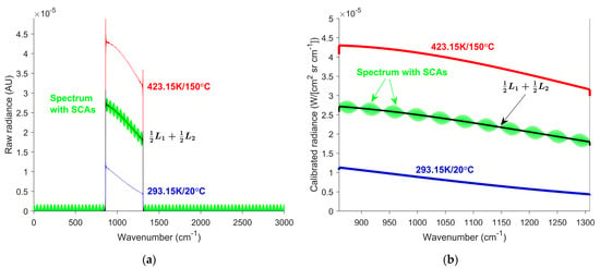
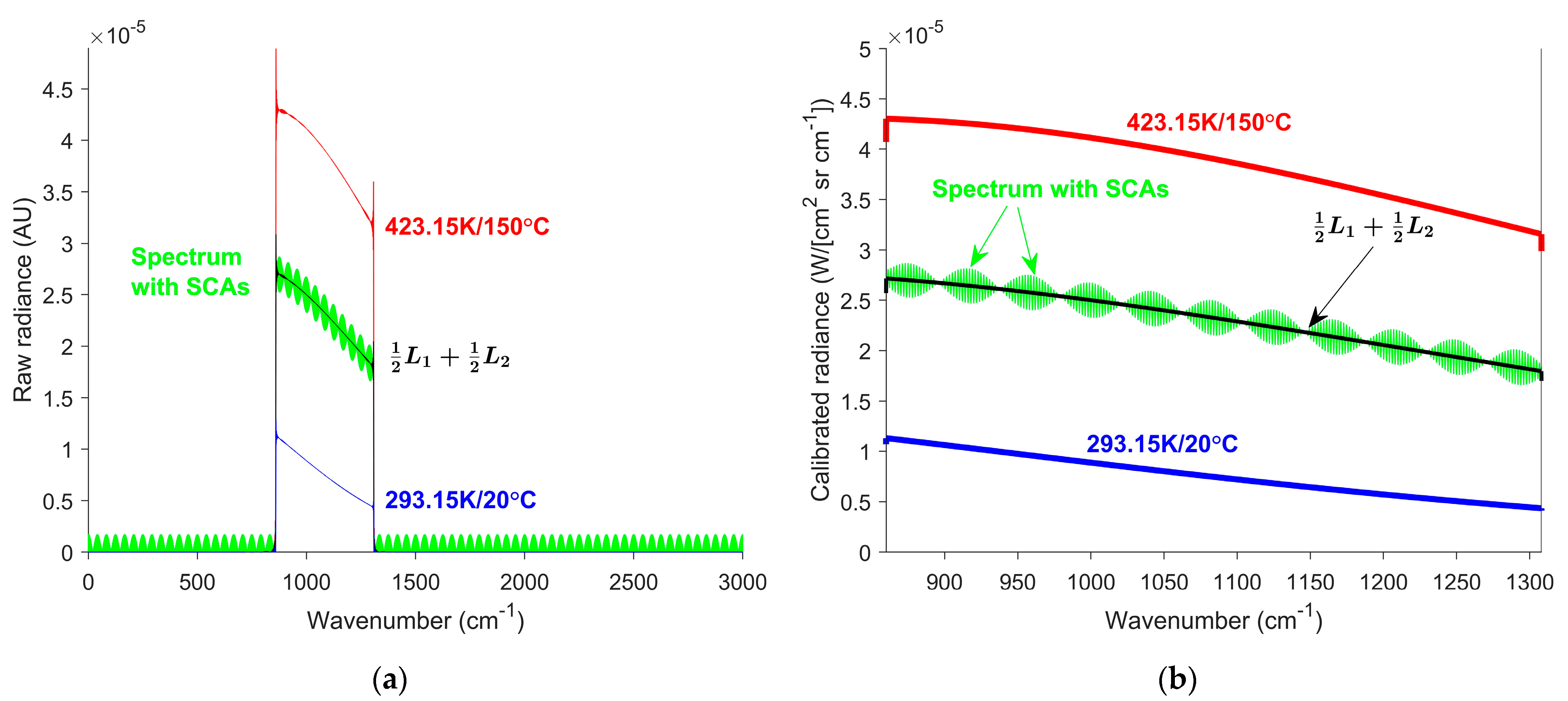
Next, consider the effects of using a realistic detector with a finite spectral response range. A flat calibration gain was applied to the simulated incident spectrum. The gain was set to one between 861 and 1306 $\mathrm{c}{\mathrm{m}}^{-1}$, and zero outside this range, corresponding to the Telops Hyper-cam LW spectral limits [47]. A calibration offset of zero was assumed for simplicity. Figure 7 shows the raw and calibrated spectra, with SCAs caused by a linear symmetric FOV transition, for an LWIR instrument.

Figure 7. (a) Raw spectrum and (b) calibrated spectrum for simulated linear symmetric FOV transition with SCAs for an LWIR instrument. The red and blue lines represent the spectra of the hot and cold blackbodies, respectively. The green line represents the calibrated spectrum. The black line represents the ZPD spectrum.

When comparing the SCAs in Figure 7 to those in Figure 4, the SCAs appear smaller when the detector gain is taken into account. This result is expected since much of the signal lies outside the detector’s response range, as shown in Figure 7a. A reduced signal results in a smaller interferogram offset, which, in turn, reduces the magnitude of the SCAs. Typically, detectors will not have the sharp cut-off shown in Figure 7a. Most detectors have some response outside their stated range, and this additional signal can contribute to the interferogram offset and thus to SCAs. Instruments with narrower spectral ranges and sharper cut-offs are expected to exhibit smaller SCAs than those with broader ranges and gradual roll-offs.

Several scenarios were simulated, in which each scenario changes a parameter compared to the linear symmetric scenario analyzed in Figure 3, Figure 4 and Figure 5. For each scenario, the calibrated spectrum containing SCAs was compared to the ZPD spectrum to calculate the NRMSE before and after correction. The asymmetric case is shown in Figure 6. The LWIR gain case is shown in Figure 7. Simulating 16 cm⁻¹ resolution is associated with an interferogram with a smaller MOPD. The one-sided interferogram eliminates all but 50 measurements near ZPD on the positive side of the OPD axis. The quadratic case replaces the linear transition with a quadratic transition, still beginning with the FOV filled by the cold blackbody and ending with the FOV filled by the hot blackbody. Lastly, no transition was used as a control to see the effect of the correction method on data without transitions. The NRMSE values, before and after applying the SCA corrections, are summarized in Table 1.

Table 1. Simulated NRMSE before and after SCA correction.

Transition/Setting	NRMSE Pre-Correction	NRMSE Post-Correction
Linear symmetric	10.29	$3.21\times {10}^{-8}$
Linear Asymmetric	5.27	$2.34\times {10}^{-7}$
Linear symmetric (LWIR Gain)	0.14	$2.84\times {10}^{-4}$
Linear symmetric ($16 \mathrm{c}{\mathrm{m}}^{-1}$ resolution)	2.52	$1.10\times {10}^{-5}$
Linear symmetric (One-sided interferogram)	5.65	$4.75\times {10}^{-6}$
Quadratic symmetric	2.24	$9.27\times {10}^{-8}$
No transition	$3.19\times {10}^{-10}$	$3.19\times {10}^{-10}$

The magnitude of SCAs decreases when the interferogram offset is smaller, such as when the smaller detector has a limited spectral range. Additionally, SCAs are reduced when the interferogram offset is estimated more accurately. This occurs when the OPD range is smaller, as in one-sided interferograms or worse spectral resolution. SCAs are prominent at a low wavenumber, which is consistent with the sinc relationship described in Equation (24) and the low-frequency changes in the interferogram offset.

For each transition examined, the correction significantly improves the NRMSE. The largest remaining error occurs in the LWIR case. This outcome is expected, as some errors near the lower and upper bounds of the detector’s spectral range result from the discontinuity there. This result is due to Gibbs phenomena, which commonly arise in FTS measurements around sharp spectral cut-offs [48]. Importantly, applying the correction to a blackbody measurement without transition does not increase the error. Therefore, the correction technique can be confidently applied to datasets both with and without transitions. The correction provides substantial improvement when SCAs are present and does not degrade performance when SCAs are not present. The simulated results align with theoretical predictions. First, the calibrated spectrum is centered on the spectrum observed at ZPD. Second, SCAs are significant, resulting in increased NRMSE. Finally, correcting the interferogram offset estimation effectively removes SCAs, leading to substantial improvements in NRMSE. Based on these results, similar improvements are anticipated in the experimental measurements.

3.2. FOV Transition Experiment Results

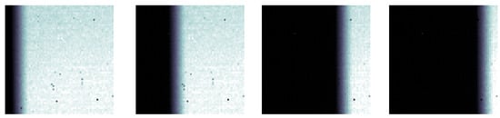
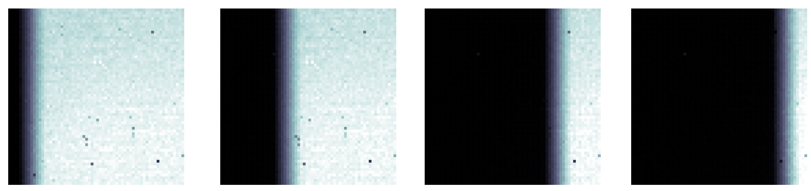
Each Telops Hyper-cam LW scan produced a double-sided interferogram for every pixel, resulting in 4096 measured interferograms for the 64 × 64 pixel array, each with 6320 discrete measurements. With these settings, the Hyper-cam requires two seconds to collect an interferogram hypercube; however, for the full 320 × 256 pixel array, a full minute can be required. These measured interferograms were processed into calibrated spectra both with and without SCA correction. For the translation stage and hyper-cam settings used, ten scans were collected while the paper transitioned the hyper-cam FOV. In the first scan, the entire FOV was filled by the blackbody. In the last scan, the entire FOV was filled by the paper. The intermediate scans captured the gradual transition. The band radiance of each pixel from each scan provides a clear indication of the paper’s position, as shown in Figure 8.

Figure 8. Band radiance images from a from the Telops Hyper-cam LW as a room-temperature paper linearly transitions across a 423 K (150 °C) blackbody. Each frame corresponds to a different interferogram scan during transition. The black speckles are caused by bad pixels on the detector array, which is known to occur with Telops Hyper-cams [49].

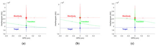
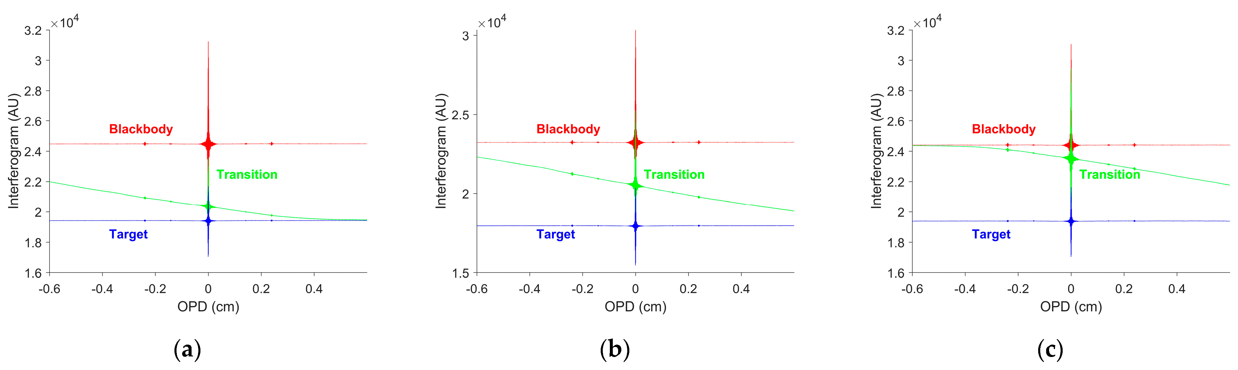
As the paper transitions across the FOV, three potential situations arise for each individual pixel. The first situation is that the blackbody fills the pixel’s FOV at the start and end of the scan. The next situation is that the paper fills the pixel’s FOV at the start and end of the scan. In these two situations, no SCAs are expected as the scene remains constant. Lastly, the pixel may start or end with some combination of blackbody and paper in its FOV. Pixels in this last situation are expected to have SCAs. These pixels occur near the paper–blackbody boundary, which appears as a gray area between the bright blackbody and dark paper in Figure 8. Measured interferograms for three of these scenarios are shown in Figure 9.

Figure 9. Measured interferogram averaged from three different pixel columns during a linear FOV transition. Red corresponds to the measured interferogram from the 423 K (150 °C) blackbody. Blue represents the measured interferogram from the room-temperature paper. Green indicates the measured interferogram from the FOV transition. (a) The pixel’s FOV initially includes both paper and blackbody, then transitions to only the paper. (b) The pixel’s FOV begins and ends with a combination of paper and blackbody. (c) The pixel’s FOV starts with only the blackbody, then ends with a combination of the paper and the blackbody.

Each pixel’s FOV is slightly different, and thus, the correction method discussed in Section 2.2 and Section 3.1 is most effective when applied individually to each pixel’s interferogram. Fortunately, as shown in Table 1, applying correction to pixels without FOV transitions is not expected to decrease accuracy. The main drawback for those pixels is a slight increase in computational processing time. Taking this into account, the SCA correction methodology is applied uniformly to all pixels.

In Section 3.1, a piecewise polynomial fit was used to estimate the interferogram offset. However, applying this method to experimental data resulted in inaccurate interferogram offset estimates. In the experiment, the paper transition produced a more gradual change to the incoming signal, in contrast to the sharp target entry modeled in the simulations. This discrepancy may be due to various factors, such as optical focus, diffraction, or vibration [50]. As a result, appropriate breakpoints for the piecewise polynomial fit became challenging, leading to incorrect interferogram offset estimates. Although higher-order polynomials and additional breakpoints were tested, these configurations had to be tailored to specific cases, making the approach impractical.

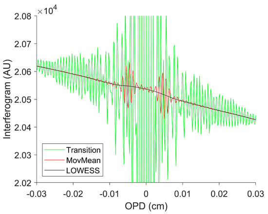
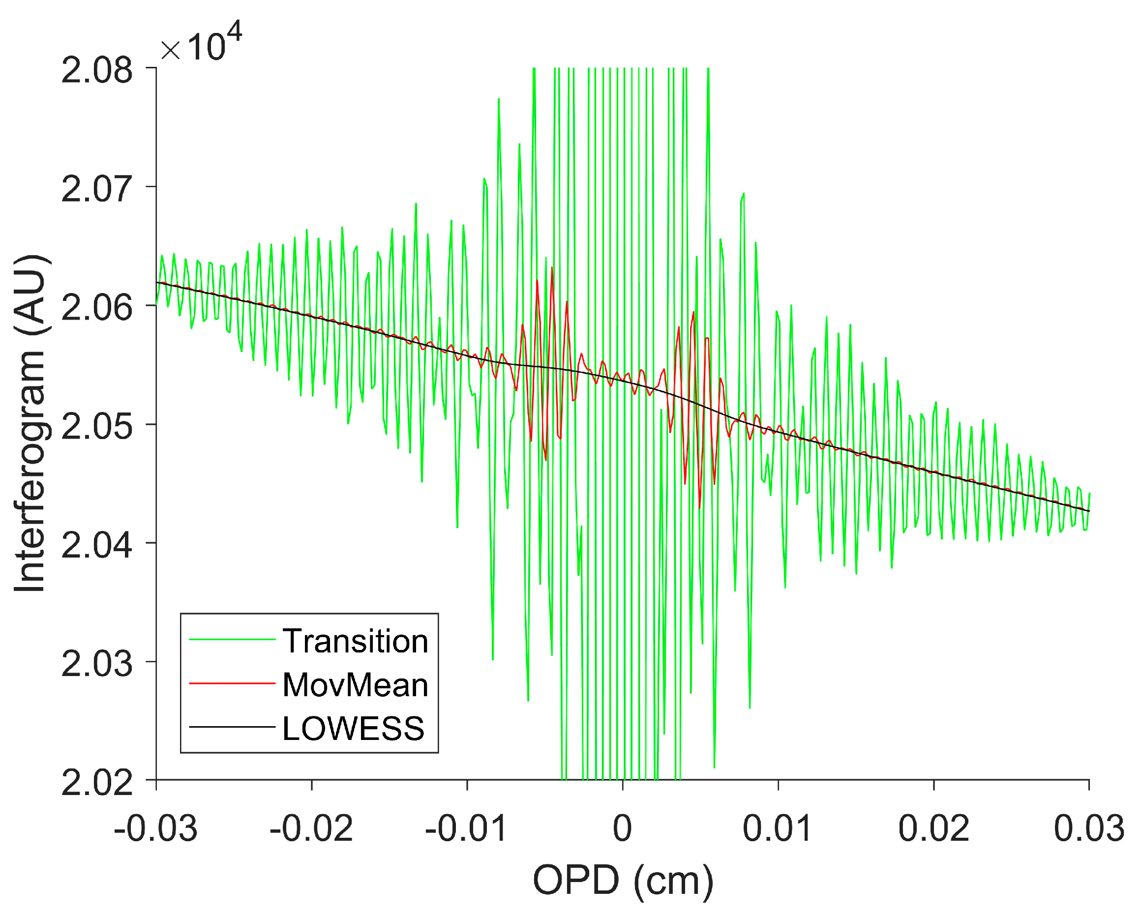
To avoid these issues, the interferogram offset estimation was performed using the built-in MATLABR 2024B smoothing function, specifically the locally weighted scatter-plot smoothing (LOWESS) option [51]. LOWESS performs weighted linear regression over small windows defined by the user [52]. Other smoothing options, such as moving mean, produced large estimate errors when the centerburst enters the window due to the large oscillations present near ZPD, as shown in Figure 10.

Figure 10. Interferogram offset estimation with smoothing near ZPD. Green indicates the measured interferogram from the FOV transition. Red indicates the interferogram offset estimate using a moving mean smoothing. Black indicates the LOWESS offset estimate. The LOWESS estimate accurately fits the interferogram offset, even across the centerburst, while the moving mean estimate contains significant variation when fitting across the centerburst.

The weighting scheme in LOWESS is particularly advantageous for fitting across the centerburst. The larger variations are dampened by the lower weights when near the window edge. As the weights increase toward the center of the window, contributions from large positive values in the centerburst are balanced by large negative values. A window size of 100 points was selected for the measured interferograms containing 6320 points. Small windows can cause an overestimate of the interferogram offset near ZPD due to the large signal spike at ZPD. This can be seen by the small upward bulge in the offset estimate near ZPD in Figure 10. While this does not result in large changes in calibrated spectra, it does cause an overestimate of the brighter target’s scene function at ZPD. Despite this, the smooth offset correction (SOC) performed similarly across a wide range of window sizes from 25 to 400 measurements, corresponding to windows both smaller and larger than the centerburst. The SOC preserves the slowly varying interferogram offset while removing the rapid fluctuations in the measured interferogram, especially around the centerburst. Moreover, SOC worked across a variety of transition speeds, eliminating the need to adjust the fit to each scenario. SOC reliably estimates the interferogram offset without requiring knowledge of the transition. SOC is an improvement over other fitting techniques that require the assumption of a scene function. The interferogram offset can then be used to infer information about the scene and the transition.

The fraction of the FOV filled by the blackbody and paper at ZPD was estimated with the data shown in Figure 9 using the following:

$${\mathrm{s}}_{\mathrm{Z}\mathrm{P}\mathrm{D}}={\displaystyle \frac{{\mathrm{I}}_{\mathrm{o},\mathrm{Z}\mathrm{P}\mathrm{D}}-{\mathrm{I}}_{\mathrm{o},1}}{{\mathrm{I}}_{\mathrm{o},2}-{\mathrm{I}}_{\mathrm{o},1}}},$$

(25)

where ${\mathrm{s}}_{\mathrm{z}\mathrm{p}\mathrm{d}}$ represents the scene function at ZPD, corresponding to the fraction of the FOV filled by the blackbody. Accordingly, $1-{\mathrm{s}}_{\mathrm{z}\mathrm{p}\mathrm{d}}$ represents the fraction of the FOV filled by the paper. ${\mathrm{I}}_{\mathrm{o},\mathrm{Z}\mathrm{P}\mathrm{D}}$ is the estimated interferogram offset at ZPD. ${\mathrm{I}}_{\mathrm{o},1}$ and ${\mathrm{I}}_{\mathrm{o},2}$ are the estimated interferogram offset of the blackbody and paper, respectively. The values of ${\mathrm{I}}_{\mathrm{o},1}$ and ${\mathrm{I}}_{\mathrm{o},2}$ are obtained by averaging the red and blue lines shown in Figure 9, respectively. Estimating these interferogram offsets requires an additional pair of measured interferograms beyond the one collected during the transition. These additional collections are taken from the same pixels as those used during the transition, but from the first and last scans, when the blackbody and paper filled the entire instrument FOV.

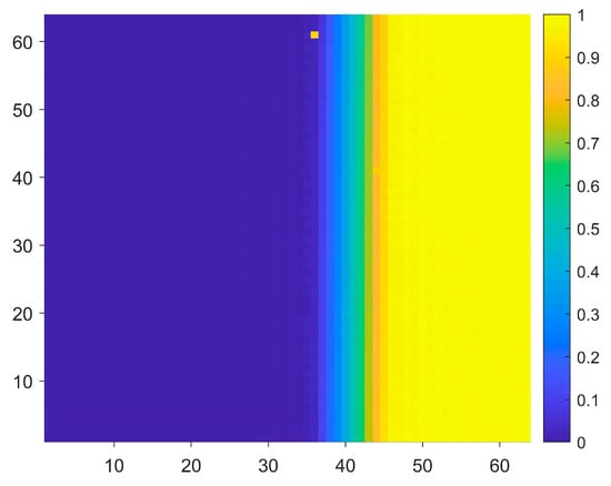
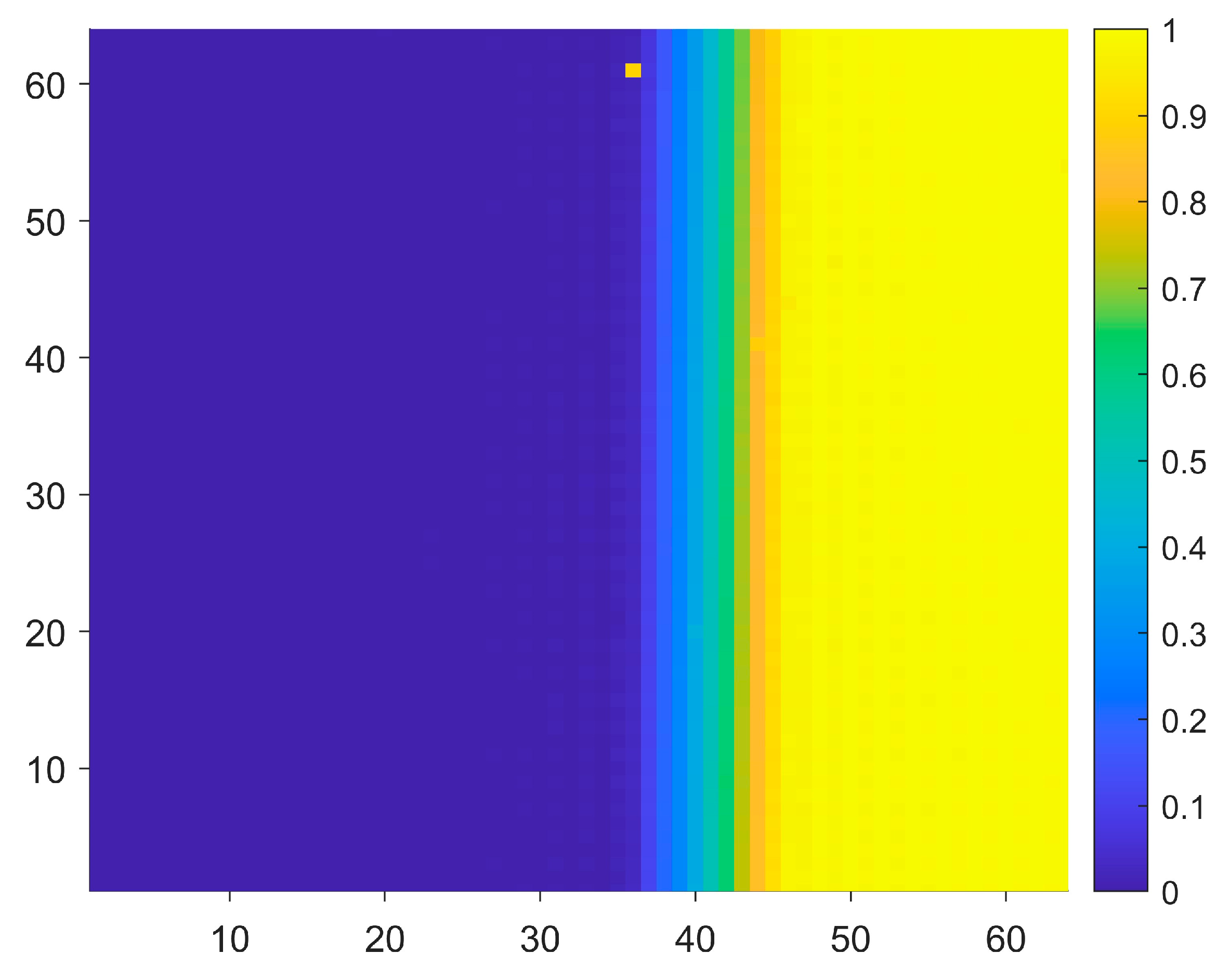
Using measurements from different scans but the same pixels yields higher accuracy than using measurements from different pixels within the same scan, since each pixel has a slightly different response. Applying Equation (26) to each pixel’s interferogram offset provides an estimate of the fraction of the FOV filled by the blackbody or paper for that pixel, as illustrated in Figure 11.

Figure 11. Estimated fraction of the FOV filled by the blackbody at ZPD. Yellow represents pixels where the FOV is filled by the blackbody at ZPD, while blue indicates pixels where the FOV is filled with paper. A small subset of pixels in between shows a combination of the blackbody and the paper.

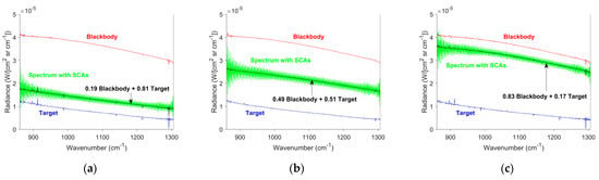
Figure 11 identifies pixels of interest where SCAs are likely to occur. Pixels that are fully filled by either the blackbody or the paper are unlikely to exhibit SCAs. In contrast, pixels that contain a mixture of both are more likely to experience transitions and, consequently, SCAs. Pixel columns 38, 43, and 48 are located on the left, center, and right sides of the transition region, respectively. Their corresponding measured interferograms are shown in Figure 9. The calibrated spectra from these pixel columns contain significant SCAs, as illustrated in Figure 12.

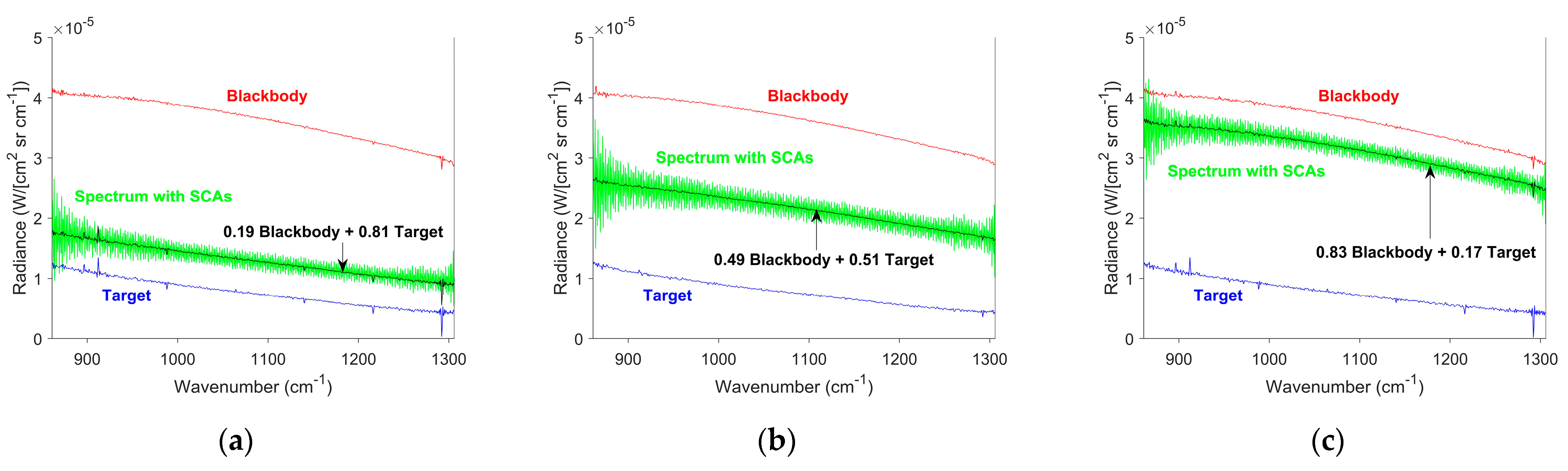
Figure 12. Calibrated spectra containing SCAs, averaged from different pixel columns from a linear FOV transition. Red indicates the calibrated spectra for the 423 K (150 °C) blackbody. Blue represents the calibrated spectra for the room-temperature paper. Green shows the calibrated spectra using standard processing techniques. Black represents the estimated spectra at ZPD. (a) The pixel’s FOV initially includes both paper and blackbody, then transitions to only the paper. (b) The pixel’s FOV begins and ends with a combination of paper and blackbody. (c) The pixel’s FOV starts with only the blackbody, then ends with a combination of the paper and the blackbody.

The calibrated spectra in Figure 12 exhibit significant SCAs when a transition is present. However, they are centered around the expected spectrum at ZPD, shown in black. This behavior is consistent with both the theoretical prediction and simulation results. The ZPD spectra are determined by the weighted average of the blackbody and paper spectra, which are determined by their respective contributions to the FOV at each pixel during the transition, given by the following:

$${\mathrm{L}}_{\mathrm{Z}\mathrm{P}\mathrm{D}}\left(\nu \right)={\mathrm{s}}_{\mathrm{Z}\mathrm{P}\mathrm{D}}{\mathrm{L}}_1\left(\nu \right)+(1-{\mathrm{s}}_{\mathrm{Z}\mathrm{P}\mathrm{D}}){\mathrm{L}}_2(\nu ),$$

(26)

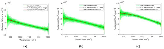
where ${\mathrm{s}}_{\mathrm{Z}\mathrm{P}\mathrm{D}}$ is given by Equation (26) and shown in Figure 11, ${\mathrm{L}}_1(\nu )$ is the calibrated spectrum of the blackbody shown in red in Figure 12, and ${\mathrm{L}}_2(\nu )$ is the calibrated spectrum of the paper shown in blue in Figure 12. Correcting the interferogram offset estimate using the smoothed measured interferogram significantly reduces SCAs, as demonstrated in Figure 13.

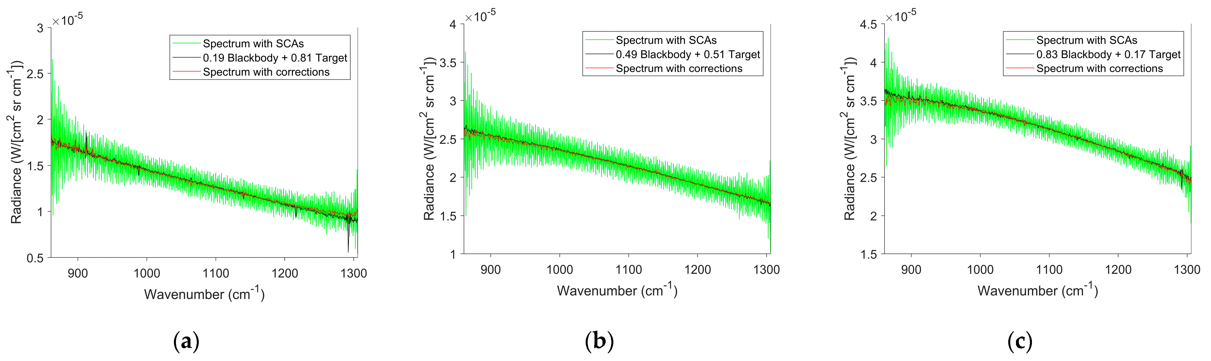
Figure 13. Calibrated spectra with SCAs and after SOC, averaged from different pixel columns from a linear FOV transition. Green shows the calibrated spectra using standard processing techniques. Black represents the estimated spectra at ZPD. Red represents the corrected spectra after improving interferogram offset estimation. (a) The pixel’s FOV initially includes both paper and blackbody, then transitions to only the paper. (b) The pixel’s FOV begins and ends with a combination of paper and blackbody. (c) The pixel’s FOV starts with only the blackbody, then ends with a combination of the paper and the blackbody.

The expected and corrected spectra are nearly indistinguishable in Figure 13, indicating that SOC is effective on experimental data. Since SCAs are centered on the ZPD spectrum, smoothing the data produces a similar effect. However, smoothing the spectrum also smooths sharp spectral features present in the data. In contrast, SOC operates on the interferogram, preserving spectral features while eliminating SCAs. The NRMSE was calculated for both uncorrected and corrected spectra shown in Figure 13, using the expected spectra at ZPD as truth. The average and standard deviation of NRMSEs for each column are shown in Table 2.

Table 2. Experimental NRMSE before and after SCA correction.

Pixel Set	NRMSE Pre-Correction	NRMSE Post-Correction
Figure 13a	$0.12\pm 0.01$	$0.047\pm 0.00$5
Figure 13b	$0.16\pm 0.02$	$0.049\pm 0.00$4
Figure 13c	$0.12\pm 0.01$	$0.049\pm 0.00$8
No transition	$0.051\pm 0.007$	$0.051\pm 0.007$

Prior to SOC, SCAs caused significant errors in the calibrated spectra. The NRMSE was highest in the center of the transition region, where the change in interferogram offset is greatest. These errors are comparable to the simulated predictions for an LWIR instrument. After applying the SOC, the NRMSE values were reduced to levels similar to those observed in measurements without any FOV transition. SOC was applied on a per-pixel basis across the full 64 × 64 array, and the NRMSE values before and after correction are shown in Figure 14.

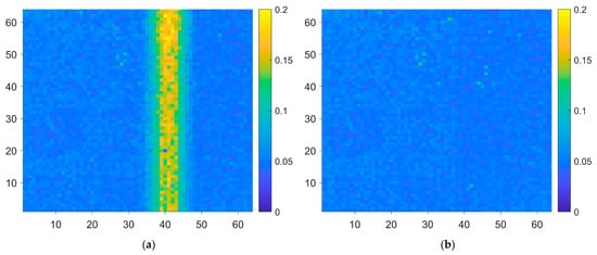
Figure 14. (a) NRMSE calculated for each pixel prior to SOC. The highest error appears in the yellow band around column 40, corresponding to the region where the FOV transitions from blackbody to paper. (b) NRMSE calculated for each pixel after SOC. The elevated error around column 40 has been effectively eliminated, resulting in consistent NRMSE values across the entire FOV.

As expected, pixels that observed either the paper or the blackbody for the duration of the interferogram exhibited minimal error. In contrast, pixels that experienced a transition between the two demonstrated significant errors due to SCAs. After applying SOC, all pixels exhibited low error levels. This demonstrates that SOC effectively reduced SCA-related errors without introducing additional errors in pixels that were not affected by SCAs.

4. Discussion

This work experimentally confirmed Kick’s theoretical prediction that the measured spectrum reflects scene conditions when ZPD occurs [12]. Furthermore, it demonstrated that this prediction holds under a wider range of conditions than the linear symmetric transition previously examined by Kick. Additionally, this study provides a theoretical basis for experimentally observed SCAs and demonstrates that they can introduce substantial errors into FTS spectra.

The discrepancy between previous theoretical predictions and experimental observations of SCAs can be attributed to differences in how the interferogram offset is estimated. Previous authors based their theoretical development on the interferogram without offset. SCAs arising from incorrect interferogram offset estimation were not considered. SCAs were found to be directly proportional to the Fourier transform of the interferogram offset estimate error. Since SCAs are centered on the ZPD spectrum, researchers often dismiss them as noise. Smoothing the spectra can mitigate SCAs, but it also smooths spectral features. Ongoing efforts aim to compare SCA mitigation using SOC to conventional noise reduction techniques. Correcting the interferogram offset estimate removes SCAs while preserving the underlying spectrum.

SCAs are more pronounced when the interferogram offset error is large. Brighter targets will produce larger SCAs than dimmer targets. Detectors with broader spectral response ranges will exhibit larger SCAs than those with narrower ranges. Measurements with larger MOPDs will show larger SCAs than those with smaller MOPDs. Correspondingly, measurements with better spectral resolution will contain larger SCAs than those with worse spectral resolution. Transitions across targets with a larger temperature difference will result in larger SCAs than transitions across targets with smaller temperature differences. Lastly, SCAs are more significant at lower wavenumbers than at higher wavenumbers.

The experiment confirmed the expectations from simulations that the observed spectra were centered on the ZPD spectra. Similarly, the experiment confirmed that SCAs were superimposed on the ZPD spectra. Unfortunately, the polynomial fitting technique used in the simulations was incompatible with the experimental transitions. While sharp transitions from one target to another were possible in the simulations, such transitions were more gradual in the experiment and not well represented by polynomial fits. The development of SOC overcame these challenges when determining the interferogram offset. SOC uses LOWESS for interferogram offset estimation. This is a standard smoothing technique and is easily implementable. SOC correctly predicts the interferogram offset across the entire measured interferogram, including the large variations around ZPD. This is particularly advantageous as many smoothing techniques have significant problems near ZPD. Furthermore, the SOC interferogram offset estimate provides information about changes in brightness within the FOV. This means that SOC provides additional information about the scene change that previously had to be assumed or known to properly fit the interferogram offset. By allowing for a variable interferogram offset estimate, SOC effectively eliminates SCAs from the resulting spectrum. SOC has been validated through experiments, showing a reduction in error, as measured by NRMSE, to levels comparable to those expected in the absence of SCAs. Applying SOC when scene changes are not present does not decrease accuracy. SOC is simple to implement, provides transition information, significantly reduces SCAs, and preserves accuracy when scene changes are not present.

Previous theoretical predictions have been experimentally confirmed. An additional source of SCAs has been theoretically established and experimentally validated. These SCAs adequately explain the discrepancies between previous experimental results and theoretical predictions. SOC is simple to implement and does not require changes to the experiment. Thus, SOC can be applied to improve the spectral accuracy of previously collected and future datasets.

This work primarily addressed smooth spectra obtained from blackbody sources. For highly structured spectra, SCAs originating from incorrect interferogram offset estimation are expected to appear and can be corrected using SOC. The interferogram offset depends on scene brightness, rather than spectral structure. This indicates that the largest source of SCAs can still be mitigated, even in highly structured spectra. However, there may still be SCAs. Kick predicted SCAs near sudden spectral changes for non-linear transitions. These SCAs are small compared to those discussed in this paper and were considered negligible by Kick [12]. Additionally, spectral accuracy near these locations is constrained by the Gibbs phenomenon. Thus, after SOC, spectral accuracy is not expected to be limited by SCAs, even for highly structured spectra.

References

- Persky, M.J. A review of spaceborne infrared Fourier transform spectrometers for remote sensing. Rev. Sci. Instrum. 1995, 66, 4763–4797. [Google Scholar] [CrossRef] [Scilit]
- Cohen, J. Introduction to Fourier Transform Spectroscopy; National Bureau of Standards: Gaithersbrug, MD, USA, 1986. [Google Scholar]
- Gebbie, H.A. Fourier transform versus grating spectroscopy. Appl. Opt. 1969, 8, 501–504. [Google Scholar] [CrossRef] [Scilit] [PubMed]
- Orson, J.A.; Bagby, W.F.; Perram, G.P. Infrared signatures from bomb detonations. Infrared Phys. Technol. 2003, 44, 101–107. [Google Scholar] [CrossRef] [Scilit]
- Slagle, S.E. Advanced Radiometry for High Discrimination Explosive Fireball Discrimination. Master’s Thesis, Air Force Institute of Technology, Wright-Patterson AFB, Dayton, OH, USA, 2009. [Google Scholar]
- Gross, K.C.; Tremblay, P.; Chamberland, M. IFTS for Turbulent Flow Field Diagnostics. In Proceedings of the Imaging and Applied Optics, Toronto, ON, Canada, 10–14 July 2011. [Google Scholar]
- Harley, J.L.; Gross, K.C. Remote Quantification of Smokestack Effluent Mass Flow Rates Using Imaging Fourier Transform Spectrometry. In Proceedings of the SPIE Defense, Security, and Sensing, Orlando, FL, USA, 3 June 2011. [Google Scholar]
- Gross, K.C.; Tremblay, P.; Bradley, K.C.; Chamberland, M.; Farley, V.; Perram, G.P. Instrument Calibration and Lineshape Modeling for Ultraspectral Imagery Measurements of Industrial Smokestack Emissions. In Proceedings of the SPIE Defense, Security, and Sensing, Orlando, FL, USA, 5–9 April 2010. [Google Scholar]
- Davis, S.P.; Mark, C.A.; James, W.B. Fourier Transform Spectrometry; Academic Press: San Diego, CA, USA, 2001. [Google Scholar]
- Holder, J.G. Polarimetric Calibration and Characterization of the Telops Field Portable Polarimetric-Hyperspectral Imager. Master’s Thesis, Air Force Institute of Technology, Wright-Patterson AFB, Dayton, OH, USA, 2014. [Google Scholar]
- Guelachvili, G. Distortions in Fourier spectra and diagnosis. In Spectrometric Techniques; Academic Press: Jovanovich, NY, USA, 1981; Volume 2. [Google Scholar]
- Kick, H.; Tank, V.; Lindermeir, E. Impact of scene changes during data acquisition in Fourier spectroscopy. J. Quant. Spectrosc. Radiat. Transf. 2005, 92, 447–455. [Google Scholar] [CrossRef] [Scilit]
- Young, A.M. Scene Change Artifacts in Fourier Transform Spectroscopy of Temporally Changing Sources. Master’s Thesis, Air Force Institute of Technology, Wright-Patterson AFB, Dayton, OH, USA, 2010. [Google Scholar]
- Gross, K.C.; Young, A.M.; Borel, C.; Steward, B.J.; Perram, G.P. Simulating systematic scene-change artifacts in Fourier-transform spectroscopy. In Proceedings of the SPIE Defense, Security, and Sensing, Orlando, FL, USA, 5–9 April 2010. [Google Scholar]
- Gross, K.C. Phenomenological Model for Infrared Emissions from High-Explosive Detonation Fireballs. Ph.D. Dissertation, Air Force Institute of Technology, Wright-Patterson AFB, Dayton, OH, USA, 2007. [Google Scholar]
- Steward, B.J. Characterization and Discrimination of Large Caliber Gun Blast and Flash Signatures. Ph.D. Dissertation, Air Force Institute of Technology, Wright-Patterson AFB, Dayton, OH, USA, 2011. [Google Scholar]
- Gordon, J.M. Shock Wave Dynamics of Novel Aluminized Detonations and Empirical Model for Temperature Evolution from Post-Detonation Combustion Fireballs. Ph.D. Dissertation, Air Force Institute of Technology, Wright-Patterson AFB, Dayton, OH, USA, 2011. [Google Scholar]
- Mitchell, H.J.; Hemmer, T.H.; Lewis, P.E.; Salvaggio, C. Effects of Temporally Changing Sources on Fourier Transform Spectrometers. In Proceedings of the Aerospace/Defense Sensing, Simulation and Controls, Orlando, FL, USA, 16–20 April 2001. [Google Scholar]
- Manzardo, M. (Air Force Institute of Technology, Wright-Patterson AFB, Dayton, OH, USA); Bussey, J. (Air Force Institute of Technology, Wright-Patterson AFB, Dayton, OH, USA). Personal communication, 2021.
- Wilson, K.A.; Diaz Ruiz, C.; Young, S.R.; Dexter, M.L.; Franz, A.L. Recombobulate correction method for oscillating scene change artifacts in longwave infrared Fourier transform spectroscopy spectra. Appl. Opt. 2025, 64, E20–E27. [Google Scholar] [CrossRef] [Scilit] [PubMed]
- Moore, E.A.; Gross, K.C.; Bowen, S.J.; Perram, G.P.; Chamberland, M.; Farley, V.; Gagnon, J.; Laguex, P.; Villemaire, A. Characterizing and Overcoming Spectral Artifacts in Imaging Fourier-transform Spectroscopy of Turbulent Exhaust Plumes. In Proceedings of the SPIE Defense Security and Sensing, Orlando, FL, USA, 13–17 April 2009. [Google Scholar]
- Tremblay, P.; Gross, K.C.; Farley, V.; Chamberland, M.; Villemaire, A.; Perram, G.P. Understanding and Overcoming Scene-change Artifacts in Imaging Fourier-transform Spectroscopy of Turbulent Jet Engine Exhaust. In Proceedings of the SPIE Optical and Engineering Applications, San Diego, CA, USA, 2–6 August 2009. [Google Scholar]
- Tremblay, P.; Savary, S.; Rolland, M.; Villemaire, A.; Chamberland, M.; Farley, V.; Brault, L.; Giroux, J.; Allard, J.; Dupuis, E.; et al. Standoff Gas Identification and Quantification from Turbulent Stack Plumes with an Imaging Fourier-transform Spectrometer. In Proceedings of the Advanced Environmental, Chemical, and Biological Sensing Technologies VII, Orlando, FL, USA, 5–9 April 2010. [Google Scholar]
- Albrecht, E.M.; Jensen, A.M.; Jensen, E.K.; Wilson, K.A.; Plummer, M.K.; Key, J.A.; O’keefe, D.S.; Chun, F.K.; Strong, D.M.; Schuetz-Christy, C.P. Near-simultaneous observations of a geosynchronous satellite using multiple telescopes and multiple remote sensing signatures. J. Astronaut. Sci. 2022, 69, 120–138. [Google Scholar]
- Mertz, L. Auxiliary computation for Fourier spectrometry. Infrared Phys. 1967, 7, 17–23. [Google Scholar] [CrossRef] [Scilit]
- Griffiths, P.R.; de Haseth, J.A. Theoretical Background. In Fourier Transform Infrared Spectrometry, 2nd ed.; John Wiley and Sons: Hoboken, NJ, USA, 2007; pp. 19–56. [Google Scholar]
- Bell, R.J. Introductory Fourier Transform Spectroscopy; Academic Press: New York, NY, USA, 1972. [Google Scholar]
- Herres, W.; Gronholz, J. Understanding FT-IR Data Processing; Bilkent University: Ankara, Turkey, 1984. [Google Scholar]
- Gaskill, J.D. Linear Systems, Fourier Transforms, and Optics; John Wiley and Sons: New York, NY, USA, 1978. [Google Scholar]
- Ebel, A.; Wolfgang, D.; Leibfritz, D. Effects of zero-filling and apodization on spectral integrals in discrete Fourier-transform spectroscopy of noisy data. J. Magn. Reson. 2006, 82, 330–338. [Google Scholar] [CrossRef] [Scilit] [PubMed]
- Bretzlaff, R.S.; Bahder, T.B. Apodization effects in Fourier transform infrared difference spectra. Rev. Phys. Appl. 1986, 21, 833–844. [Google Scholar] [CrossRef] [Scilit]
- Sromovsky, L.A. Radiometric errors in complex Fourier transform spectrometry. Appl. Opt. 2003, 42, 1779–1787. [Google Scholar] [CrossRef] [Scilit] [PubMed]
- Revercomb, H.E.; Buijs, H.; Howell, H.B.; LaPorte, D.D.; Smith, W.L.; Sromovsky, L.A. Radiometric calibration of IR Fourier transform spectrometers: Solution to a problem with the high-resolution interferometer sounder. Appl. Opt. 1988, 27, 3210–3218. [Google Scholar] [CrossRef] [Scilit] [PubMed]
- Dereniak, E.L.; Boreman, G.D. Infrared Detectors and Systems; Wiley: New York, NY, USA, 1996. [Google Scholar]
- Rogatto, W.D. Detectors. In The Infrared and Electro-Optical Systems Handbook; Acetta, J.A., Shumaker, D.L., Eds.; ERIM: Ann Arbor, MI, USA, 1993; Volume 3, pp. 177–286. [Google Scholar]
- Gross, K.C.; Borel, C.; White, A.; Sekai, S.; DeVasher, R.; Perram, G.P. First Imaging Fourier-transform Spectral Measurements of Detonation in an Internal Combustion Engine. In Proceedings of the SPIE Optical Engineering, San Diego, CA, USA, 1–5 August 2010. [Google Scholar]
- Bertie, J.E. Apodization and Phase Correction. In Proceedings of the NATO Advanced Study Institute, Florence, Italy, 31 August–12 September 1979; pp. 25–50. [Google Scholar]
- Otto, S.A.; Kadin, M.; Casini, M.; Torres, M.A.; Bleckner, T. A quantitative framework for selecting and validating food web indicators. Ecol. Indic. 2018, 84, 619–631. [Google Scholar] [CrossRef] [Scilit]
- Gareth, J.; Witten, D.; Hastie, T.; Tibshirani, R. An Introduction to Statistical Learning: With Applications in R, 2nd ed.; Springer: Cham, Switzerland, 2023. [Google Scholar]
- Lagueux, P.; Farley, V.; Chamberland, M.; Villemaire, A.; Turcotte, C.; Puckrin, E. Design and Performance of the Hyper-Cam, an Infrared Hyperspectral Imaging Sensor; Defense Technical Information Center: Fort Belvoir, VA, USA, 2009. [Google Scholar]
- Hyper-Cam Training: Advanced Hardware Presentation (Telops, Quebec City, QC, Canada); Wilson, K.A. (Air Force Institute of Technology, Wright-Patterson AFB, Dayton, OH, USA). Personal communication, 2013.
- Fluke Corporation. 4180 Series Precision Infrared Calibrators; Brochure; Fluke: Everett, WA, USA, 2021; p. 4. [Google Scholar]
- Brewster, M.Q. Thermal Radiative Transfer and Properties; John Wiley and Sons: New York, NY, USA, 1992; p. 56. [Google Scholar]
- Thor Labs 150 mm Linear Translation Stage with Integrated Controller, Stepper Motor. Available online: https://www.thorlabs.com/newgrouppage9.cfm?objectgroup_id=3961 (accessed on 24 September 2025).
- Petty, G.W. A First Course in Atmospheric Radiation, 2nd ed.; Sundog Publishing: Madison, WI, USA, 2006. [Google Scholar]
- Telops. Hyperspectral Imaging Systems; Brochure; Telops: Quebec City, QC, Canada, 2025; p. 4. [Google Scholar]
- Montembeault, Y.; Lagueux, P.; Farley, V.; Villemaire, A.; Gross, K.C. Hyper-Cam: Hyperspectral IR imaging applications in defense innovative research. In Proceedings of the 2nd Workshop on Hyperspectral Image and Signal Processing: Evolution in Remote Sensing, Reykjavik, Iceland, 14–16 June 2010. [Google Scholar]
- Wilbraham, H. On a certain periodic function. Camb. Dublin Math. J. 1848, 3, 198–201. [Google Scholar]
- Glimsdal, E.; Brendhagen, E.; Thomassen, J.B.; van Rheenen, A.D.; Heen, L.T. Obtaining Spectral Information from Infrared Scenarios using Hyper-spectral Cameras and Cameras with Spinning Filter Wheel. In Proceedings of the Electro-Optical Remote Sensing, Photonic Technologies, and Applications VIII: And Military Applications in Hyperspectral Imaging and High Spatial Resolution Sensing II, Amsterdam, The Netherlands, 22–25 September 2014. [Google Scholar]
- Goodman, J.W. Introduction to Fourier Optics, 4th ed.; McGraw Hill: New York, NY, USA, 2017; p. 14. [Google Scholar]
- MATLAB Help Center, Smoothdata. Available online: https://www.mathworks.com/help/matlab/ref/smoothdata.html (accessed on 9 September 2025).
- Moran, G.W. Locally-Weighted-Regression Scatter-Plot Smoothing (LOWESS): A Graphical Exploratory Data Analysis Technique. Master’s Thesis, Naval Postgraduate School, Monterey, CA, USA, 1984. [Google Scholar]
- Stipp, D. A Most Elegant Equation Euler’s Formula & the Beauty of Mathematics; Basic Books: New York, NY, USA, 2017. [Google Scholar]
- MATLAB Help Center, Sinc. Available online: https://www.mathworks.com/help/signal/ref/sinc.html (accessed on 24 September 2025).
Disclaimer/Publisher’s Note: The statements, opinions and data contained in all publications are solely those of the individual author(s) and contributor(s) and not of MDPI and/or the editor(s). MDPI and/or the editor(s) disclaim responsibility for any injury to people or property resulting from any ideas, methods, instructions or products referred to in the content. |
© 2026 by the authors. Licensee MDPI, Basel, Switzerland. This article is an open access article distributed under the terms and conditions of the Creative Commons Attribution (CC BY) license.