


Highlights
What are the main findings?
- Among the three methods for estimating daily relative humidity (RH) in China, the Random Forest (RF) model performed the best.
- The dew point temperature (), Aridity Index (AI) and day of year (DOY) were identified as the most important features for RH estimation. Model accuracy exhibited a clear spatial pattern, being higher in humid zones and lower in arid zones, and a distinct seasonal pattern, with the highest accuracy in summer.
What is the implication of the main finding?
- This study identifies the optimal method and important predictive variables, such as , AI and DOY, for achieving highly accurate RH estimation.
- The resulting high-resolution data enable the capture of subtle changes in RH caused by urban dry islands and water bodies, which is something that the existing lower datasets cannot achieve. This provides a reliable scientific basis for analyzing the role of RH in climate change and its response to climatic shifts.
Abstract
Relative humidity (RH) is an important meteorological factor that affects both the climate system and human activities. However, the existing observational station data are insufficient to meet the requirements of regional scale research. Machine learning methods offer new avenues for high precision RH estimation, but the performance of different algorithms in complex geographical environments still needs to be thoroughly evaluated. Based on Chinese observational station data from 2011 to 2020, this study systematically evaluated the performance of three methods for estimating RH: the generalized linear mixed model (GLMM), random forest (RF) and the XGBoost algorithm. The results of ten-fold cross validation indicate that the two machine learning methods are significantly superior to the traditional GLMM. Among them, RF performed the best (the determinant coefficient (R2) = 0.73, root mean square error (RMSE) = 8.85%), followed by XGBoost (R2 = 0.72, RMSE = 9.07%), while the GLMM performed relatively poorly (R2 = 0.58, RMSE = 11.08%). The model performance shows significant spatial heterogeneity. All models exhibit high correlation but relatively large errors in the northern regions, while demonstrating low errors yet low correlation in the southern regions. Meanwhile, the model performance also shows significant seasonal variations, with the highest accuracy observed in the summer (June to September). Among all features, dew point temperature () aridity index (AI) and day of year (DOY) are the main contributing factors for RH estimation. This study confirms that the RF model provides the highest accuracy in RH estimation.
1. Introduction
Relative humidity (RH) is one of the critical elements measured by meteorological stations, serving as an important parameter for atmospheric moisture content [1,2,3]. It plays a significant role in drought detection [4], evaluating various risks associated with high humidity environments [5], urban epidemiological distribution studies [6,7], and monitoring the frequent occurrence of extreme fire weather worldwide [8,9], among others. With increased global climate change, the influence of RH on atmospheric circulation [10,11,12,13], the greenhouse effect [14] and precipitation patterns [15] has become increasingly significant. Accurate RH data are crucial for various applications.
RH is typically measured directly with hygrometers, which are employed in most modern automatic meteorological stations [16,17]. Although station data offer the advantages of high accuracy and real-time availability, they also have certain limitations [18]. First, the equipment required for meteorological stations is highly accurate, which increases the cost of acquiring data [19]. Second, the spatial distribution of meteorological stations is sparse and uneven, especially in remote regions where the number of stations is limited. As a result, meteorological station data are unable to comprehensively represent the continuous spatial variation in RH. With the development of technology, reanalysis products have become reliable tools for acquiring spatially continuous RH data. The reanalysis products are generated at the global scale integrating meteorological observation data, numerical models and data assimilation techniques [20]. However, the spatial resolution of the RH data from widely used reanalysis datasets—such as the National Centers for Environmental Prediction climate forecast system version 2 (NCEP-2) and the Japanese 55-year Reanalysis (JRA-55), with resolutions of 2.5° and 1.25°, respectively [21]—is often too coarse for local areas. Hence, it is of great significance to develop a method for accurately and cost-effectively estimating RH.
Although the existing interpolation techniques can be used to generate RH maps of the study area, the accuracy of the resulting data is limited due to the uneven spatial distribution and small number of observation stations [22,23]. In response to this challenge, a lot of scholars have explored methods that utilize other high spatial resolution remote sensing data to improve the accuracy of RH estimation. For instance, it has been found that there is a strong linear correlation between precipitable water vapor (PWV) and actual vapor pressure () [24]. The saturated vapor pressure can be calculated from air temperature () using the ideal gas law and thermodynamic functions [16]. Therefore, several researchers have used the empirical relationships between air temperature and precipitable water vapor to estimate RH [16]. But the empirical models calibrated with limited data—such as those collected from small areas over only one or two years—are prone to random errors and may not be representative of conditions across broader regions. Although the method of estimating RH using land surface temperature (LST) and precipitable water vapor data is straightforward and widely applicable, its accuracy remains relatively low, with a reported root mean square error (RMSE) typically ranging from 15% to 17% [25].
Some statistical methods are frequently employed for estimating meteorological parameters. A three-stage regression-based model was proposed by Kloog et al. [26] to estimate the average daily air temperature [27]. This methodology employs a linear mixed model (LMM) framework that incorporates time as a grouping variable. The LMM not only has a simple modeling approach but also provides accurate predictions for meteorological parameters such as air temperature that follow a normal distribution. Extended from the LMM, the generalized linear mixed model (GLMM) incorporates time as a random effect, making it suitable for modeling non-normally distributed parameters such as RH [28].
In order to enhance the reliability of RH estimation, other methods have been introduced for more accurate estimation. In recent years, many machine learning methods have served as effective tools for estimating RH, valued not only for their predictive power but also for their ability to provide insights into influential variables. The RF approach was employed in estimating summer daily RH throughout China [29]. Nikolaou et al. [30] also used RF to model and estimate the RH in Germany from 2000 to 2021. The XGBoost algorithm was applied by Park et al. [31] to analyze RH data across Japan and South Korea during the 2012–2017 period. However, these studies have limitations in terms of small research areas and incomplete temporal coverage. China, with its diverse climate types, is an ideal research area and provides a unique advantage for RH estimation. The ChinaMet [32] and CDMet [33] datasets are two widely used sources of daily RH data in China. The ChinaMet dataset only takes ERA5-Land reanalysis data and meteorological station data as inputs when estimating RH. Although CDMet was developed based on multi-source auxiliary data, including longitude, latitude, altitude, slope, aspect and ERA5 reanalysis data, it still has the drawback of coarse resolution. Inevitably, they may prove less reliable in capturing many localized fine-scale variations.
To address these issues, this study compares GLMM, XGBoost and RF for RH estimation using multi-source data from 2160 meteorological stations across China. Based on this comparison, the specific objective is to develop a new 1 km resolution dataset for China and to validate it against existing products.
2. Materials and Methods
2.1. Study Area
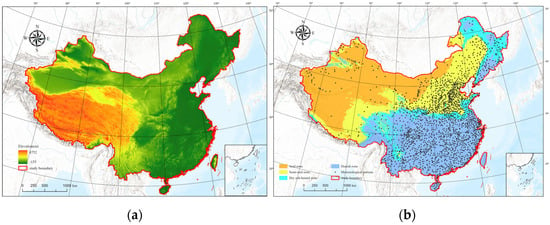
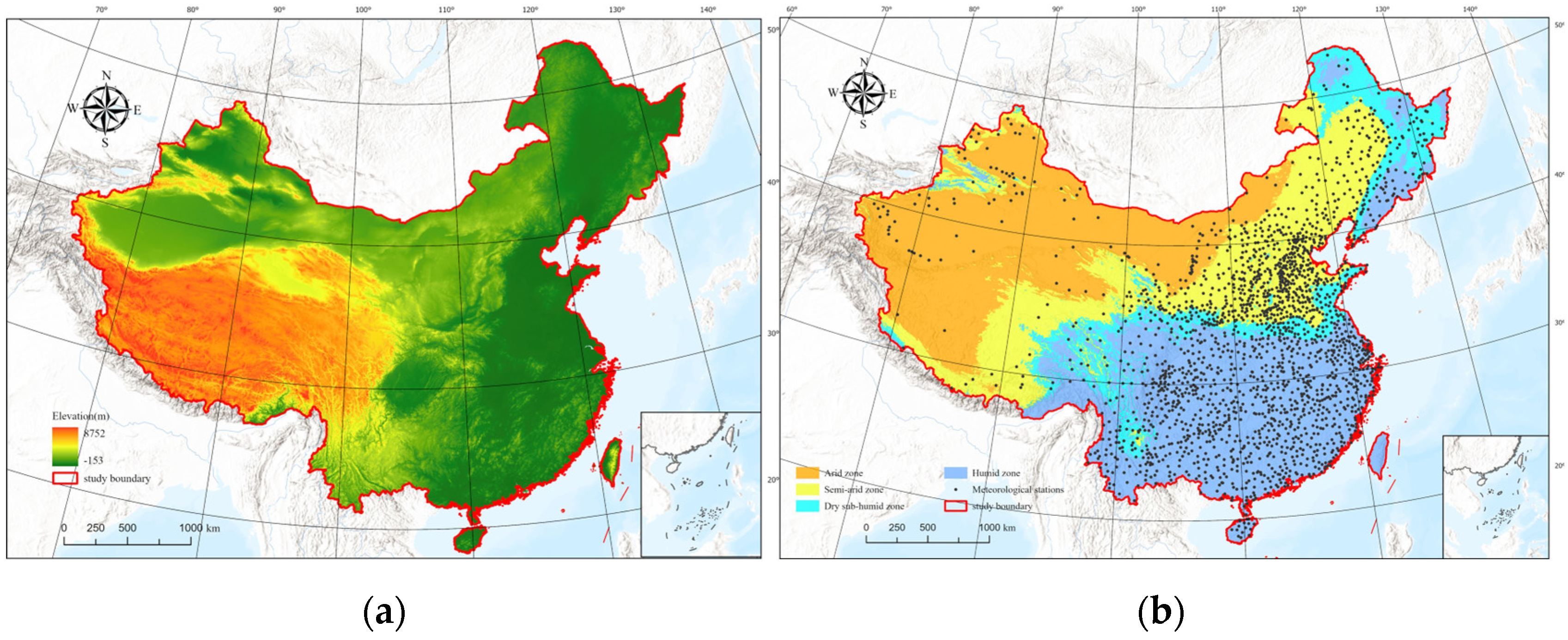
China covers an area of approximately 9,600,000 km2 and is primarily located in East Asia. It has complex terrain, and the difference in elevation within the entire study area is above 8500 m (Figure 1a). The study area exhibits pronounced spatial variations in aridity and humidity, which is classified into four climate zones—arid, semi-arid, dry sub-humid and humid—based on aridity index (AI) thresholds of 0.2, 0.5 and 0.65 (Figure 1b). Due to these complex physiographic and climatic conditions, significant variations exist in RH distribution across China. Therefore, the study of RH in China is particularly important for global studies of RH across diverse climatic regimes.
Figure 1.
Map of the study area: (a) elevation; (b) distribution of 2160 meteorological stations and climate zones.
2.2. Data
In the modeling process, we input massive amounts of daily mean RH measurements and remote sensing data across China from 2011 to 2020, which were used for model training and validation.
2.2.1. Meteorological Data
Daily mean RH measurements for 2011–2020 were obtained from the China Meteorological Data Service Centre (CMDC), the national platform for authoritative meteorological data management and services. We excluded unusual values including missing or abnormal data. After the removal of some stations, we retained data from 2160 stations for the final 2011–2020 dataset (Figure 1b).
2.2.2. Remote Sensing Data
All datasets were resampled to 1 km resolution using the nearest neighbor method. This process was crucial for the subsequent work as it ensured that all the pixel values of the raster data are aligned, thereby facilitating model predictions. The coordinate system of all the data was based on the World Geodetic System 1984 (WGS 84) (also known as EPSG: 4326).
MODIS Data
It is well-established that and dewpoint temperature () are widely used for estimating RH [16]. Previous studies have shown that MOD07_L2 and MYD07_L2 products are commonly employed to obtain and [34]. As concluded by Zhu et al. [34], the MOD07_L2 product shows a stronger correlation with observations compared to the MYD07_L2 product when extracting at the lowest vertical pressure level. Hence, it is reasonable to prioritize the atmospheric temperature profile and atmospheric moisture profile from the MOD07_L2. The product has a spatial resolution of 5 km. The MOD07_L2 product provides atmospheric profiles across 20 standardized pressure levels (1000, 950, 920, 850, 780, 700, 620, 500, 400, 300, 250, 200, 150, 100, 70, 50, 30, 20, 10 and 5 hPa) [35]. There are generally two approaches for its processing. One is to extract at the lowest vertical pressure level, which is the LVP method [36,37,38]. The other is to interpolate at the two lowest pressure levels to obtain the near-surface , which is the ALR method [39,40]. We employed the second method. The mathematical formula is expressed as:
where the denotes the or retrieved by LVP, and represents or at the lowest vertical pressure level of MOD07_L2 product. The near-surface estimates of or obtained via the adiabatic lapse rate (ALR) method are denoted as . Furthermore, and represent the retrieved (or ), respectively, at the pressure level immediately above the lowest available pressure level (); indicates surface pressure, is the vertical height difference between these two pressure levels, is air density, and g is gravitational acceleration.
In this study, Google Earth Engine was used to download the MOD09GAv061 product [30]. The red band and near-infrared band in the MODIS Surface Reflectance product were used to calculate the daily normalized difference vegetation index (NDVI), as follows [41]:
where represents the NDVI value in the grid cell corresponding to site i on day j; denotes the near-infrared band reflectance of pixel i on day j, and indicates the red band reflectance of pixel i on day j.
Aridity Index Data
The AI is defined as the ratio of precipitation to potential evapotranspiration. Developed based on the WorldClim global climate dataset, it serves as an indicator for assessing drought conditions [42], with lower values corresponding to more arid environments. This dataset features a spatial resolution of approximately 1 km and is accessible through the CGIAR-CSI Geoportal (https://cgiarcsi.community, accessed on 15 March 2025).
Elevation Data
The elevation data used in this study were derived from GTOPO30, a global digital elevation model (DEM) with a horizontal grid spacing of 30 arc seconds (approximately 1 km). The dataset was sourced from the U.S. Geological Survey’s Center for Earth Resources Observation and Science (EROS) (https://www.usgs.gov/centers/eros, accessed on 17 March 2025).
2.3. Methods
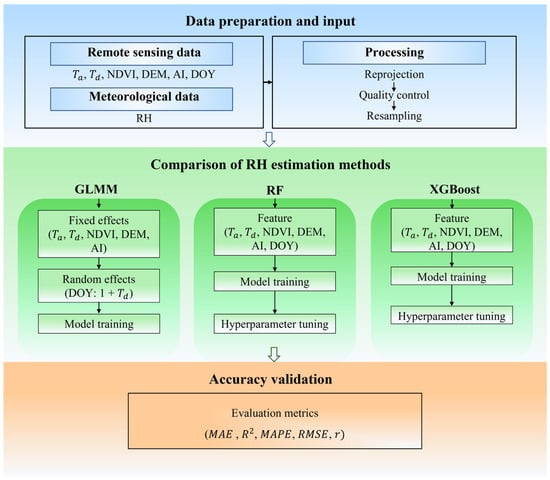
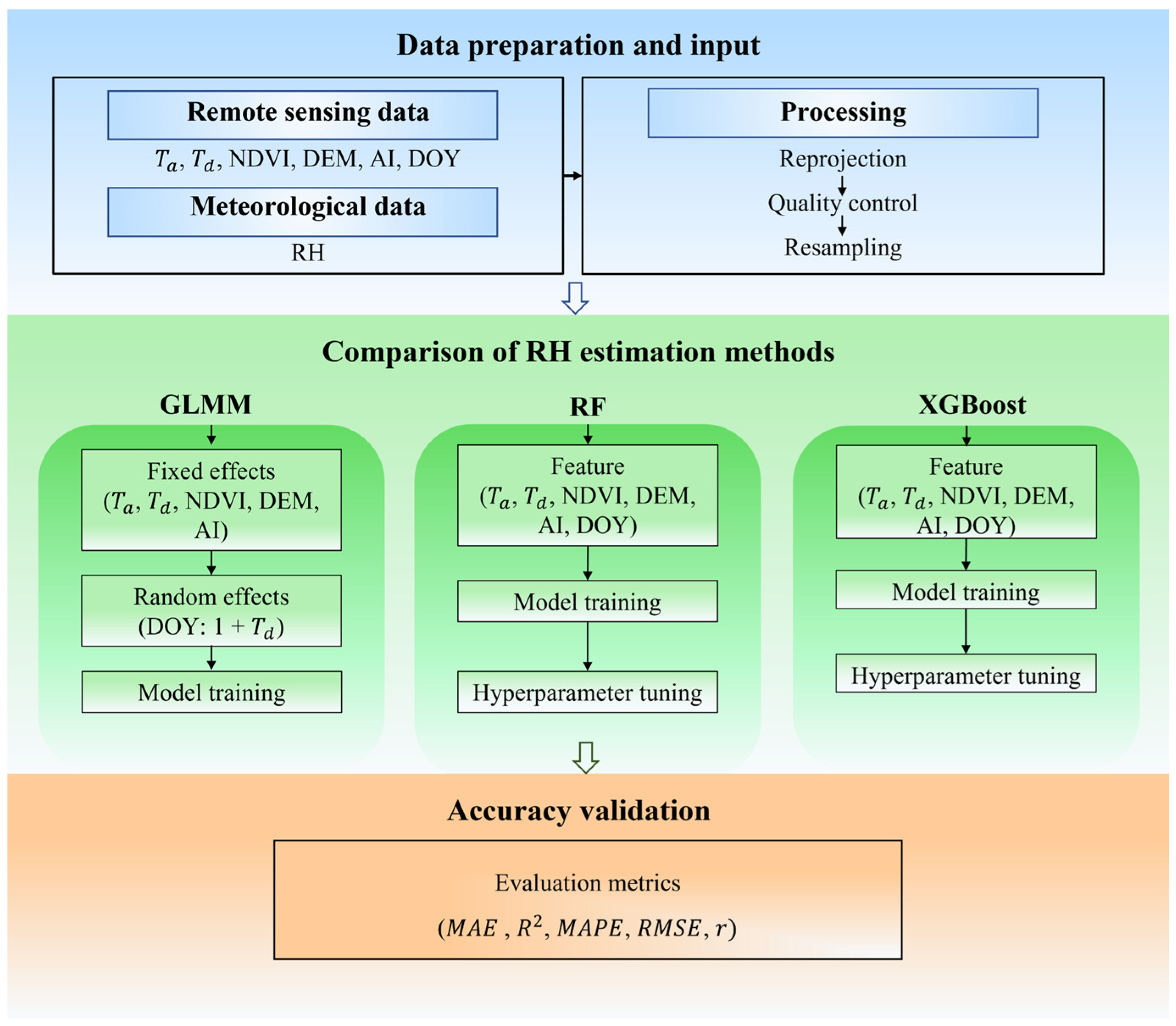
In this study, the daily mean RH was predicted at a spatial resolution of 1 km. To achieve this, multiple estimation approaches were employed and systematically compared. The high precision, low error rates and simplicity of the LMM have made them standard tools for temperature estimation. Building on this foundation, GLMMs were incorporated to characterize the daily relationship between and RH, thereby enhancing the accuracy of RH estimation. In addition, to improve estimation performance and compare the performance of different methods, this study also implemented two machine learning algorithms—RF and XGBoost. Through systematic comparison of the three approaches, this study aimed to identify the optimal method for RH estimation. All analyses were conducted using Python 3.7. The flowchart of this study is shown in Figure 2.
Figure 2.
The flowchart of this research.
2.3.1. GLMM
In recent years, the LMM has been widely used to estimate near-surface air temperature [27,43], requiring the response variable to follow the normal distribution. The GLMM can effectively address this constraint by supporting non-normal response distributions [44,45,46]. In this study, the daily mean RH ranged between 0 and 100. Before modeling, each value was scaled by a factor of 1/100, where 0 was replaced with 0.001 and 1 with 0.999, thereby transforming the range to (0, 1). This transformed variable has been confirmed by Yao et al. [28] to follow a Beta distribution. In addition to the commonly used parameters or for estimating RH provided by MOD07_L2, we also incorporated additional auxiliary variables [47], such as NDVI, DEM, AI and day of year (DOY), where DOY is used to achieve the daily slope and intercept of the relationship between and RH.
represents the RH observation at the grid cell i on day j; and stand for the fixed and the random intercepts, respectively; stands for the daily measurement at the grid cell i on day j; and stand for the fixed and the random slopes, respectively; stands for the daily measurement at the grid cell i on day j; stands for the daily NDVI measurement at the grid cell i on day j; stands for the elevation at grid cell i; stands for the AI value at grid cell i; is the error term at grid cell i on day j.
2.3.2. Machine Learning
The RF and XGBoost are well-known machine learning algorithms in various regression tasks [48,49,50], owing to strong generalization capabilities and low prediction errors. These advantages make them particularly effective for capturing complex nonlinear relationships [51,52]. Critically, beyond their predictive power, both methods offer a high degree of interpretability, enabling the discernment of which features most significantly influence RH estimates. The RF algorithm operates by constructing multiple decision trees and calculates its final result by averaging the prediction of all decision trees [53], while XGBoost adopts a boosting strategy, iteratively adding trees that minimize the residual errors of previous models, with the final prediction being a weighted sum of all tree outputs [54]. Both RF and XGBoost attain the optimal performance of the model by setting appropriate parameters through the grid search method. Table 1 presents the optimized parameters. The selected features in the two methods are similar to the GLMM approach used in this study, with the only difference being that DOY was included as one of the input features in the training process.
Table 1.
Optimized parameters for RF and XGBoost.
2.3.3. Important Feature Selection
The variations in RH are driven by different climatic and environmental factors [55,56]. Based on the inclusion of and , other available variables were selected for the model. DEM, NDVI and DOY are commonly used as auxiliary variables for estimating remote sensing meteorological data [57]. Additionally, since is approximately equal to [58], obtaining high-precision is often achieved by calculating it from [59]. Within the same climate zone, the correction factors between and are also similar. The climate zones can be divided based on the aridity index. Some scholars have estimated by introducing AI to calculate the correction factors in the study area. Therefore, AI was also incorporated into the model as an independent variable in this study [34,60]. To ensure the suitability of input features for modeling, this study analyzed the Pearson correlation coefficient (PCC) and variance inflation factor (VIF) among independent variables. PCC was used to evaluate the degree of linear correlation between variables (with |r| ≥ 0.8 considered indicative of high correlation), while VIF was employed to detect multicollinearity (where VIF > 10 generally suggests severe multicollinearity). For further examination of feature interactions and assessment of each feature’s contribution to model predictions, the Shapley Additive Explanation (SHAP) method was utilized.
2.3.4. Model Performance Evaluation
The model was validated through 10-fold cross validation (CV), and the entire dataset was randomly divided into 10 folds by site to assess its generalization ability of model on unknown sites. Then, nine folds were selected as the training set to train the model, and the remaining fold was used for validation. This process was repeated ten times, ensuring that each fold could validate once. Our dataset comprises processed records from 2011 to 2020. Notably, the final model was trained on the complete annual datasets.
2.3.5. Comparison with ChinaMet and CDMet
In order to further evaluate the accuracy of the estimated RH, it was decided to include two commonly used datasets, ChinaMet [32] and CDMet [33], for validation in this study. The ChinaMet can be downloaded from National Cryosphere Desert Data Center (https://www.ncdc.ac.cn/, accessed on 25 March 2025). Its spatial resolution is 0.01°, but its input data are only the low-resolution ERA5-Land reanalysis data. The CDMet is a 4 km daily gridded meteorological dataset for China. The two datasets are all widely used, so it is necessary to compare them. To ensure a consistent and fair comparison, daily RH values from all three datasets (the estimated values, ChinaMet and CDMet) were extracted for identical monitoring stations. The data were then precisely matched by corresponding stations and timestamps for comparison.
3. Results
3.1. Model Performance
To construct a reliable RH estimation model and avoid multicollinearity among predictor variables, the PCC was applied to calculate the correlations between each feature, and multicollinearity was quantified by computing the VIF for each variable, as described in Section 2.3.3. The results are presented in Table 2, which shows that the highest correlation exists between Ta and Td (r = 0.798), consistent with meteorological principles and remaining below the threshold of 0.8. RHU exhibits a moderate positive correlation with Td, AI, and NDVI, and a weak negative correlation with DEM, indicating the potential explanatory power of these variables for relative humidity estimation. In this study, the VIF values of all predictor variables were below 10, and therefore all variables were retained for subsequent modeling to avoid omitting important influencing factors.
Table 2.
Correlation matrix and VIF values of predictor variables.
Table 3 presents the overall results of CV for the GLMM, RF and XGBoost models for the period 2011–2020. Overall, the average R2 values of the three methods were 0.58, 0.73 and 0.72, respectively; the average RMSE values were 11.08%, 8.85% and 9.07%, respectively; and the mean absolute error (MAE) values were 8.79%, 6.89% and 7.09%, respectively. In general, all evaluation metrics demonstrated that the accuracy of RF was superior, indicating its advantage for this specific regression task. Furthermore, the results demonstrated that RF consistently outperformed XGBoost across all performance metrics throughout the study period. Both machine learning methods achieved significantly higher accuracy than the GLMM. Specifically, compared to the GLMM, RF achieved a relative improvement of approximately 26% in R2 and a 21% reduction in error. This substantial enhancement is consistent with the strong predictive capability of machine learning approaches. It is worth emphasizing that all models exhibited the lowest RMSE and MAE between 2016 and 2017, whereas errors were comparatively higher in 2019. Given that the number of monitoring stations remained stable each year (ranging from 2133 to 2142), these performance fluctuations are more likely attributable to interannual meteorological variability rather than changes in spatial data coverage.
Table 3.
Performance measures of the three models during 2011–2020.
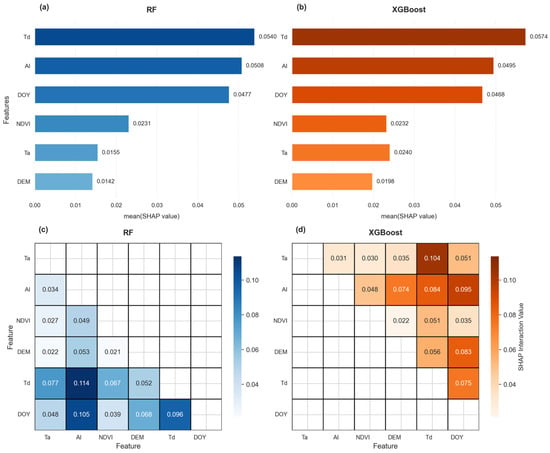
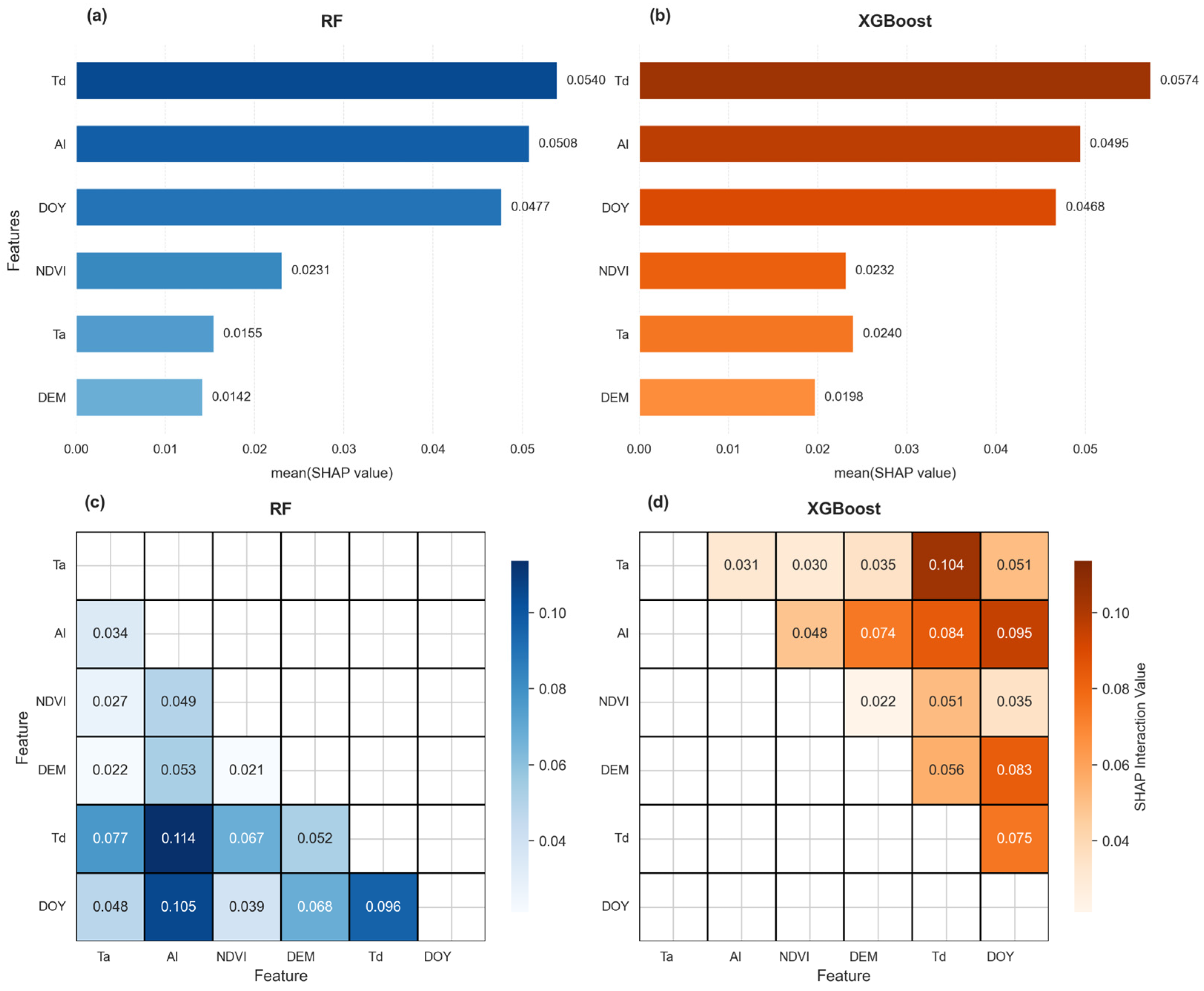
This study analyzed the feature importance and interaction effects among various factors using the SHAP method. The results indicated that the RF and XGBoost models exhibited strong agreement in identifying the key drivers, while differences emerged in their interaction patterns. Regarding feature importance (Figure 3a,b), Td contributed most significantly in both models, followed by AI and DOY, which confirmed that these three variables were the core predictors. In contrast, NDVI, Ta and DEM showed substantially lower importance, indicating their limited influence on model performance. Figure 3c,d illustrate the SHAP interaction analysis, which further revealed nonlinear associations between features. In the RF model, the Td–AI interaction was most prominent, followed by DOY–AI. In the XGBoost model, the Ta–Td interaction was more pronounced. Despite these differences in specific interaction strengths, Td, AI and DOY consistently interacted strongly with other variables in both models, reinforcing their central role in shaping predictions.
Figure 3.
SHAP analysis of RF and XGBoost: (a) RF feature importance; (b) XGBoost feature importance; (c) RF interaction matrix; (d) XGBoost interaction matrix.
3.2. Spatiotemporal Analysis of Estimation Accuracy
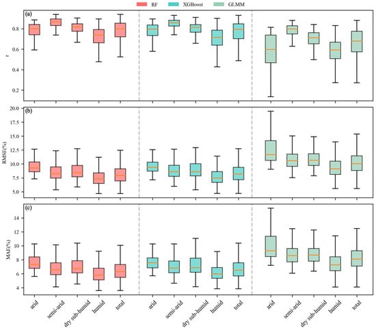
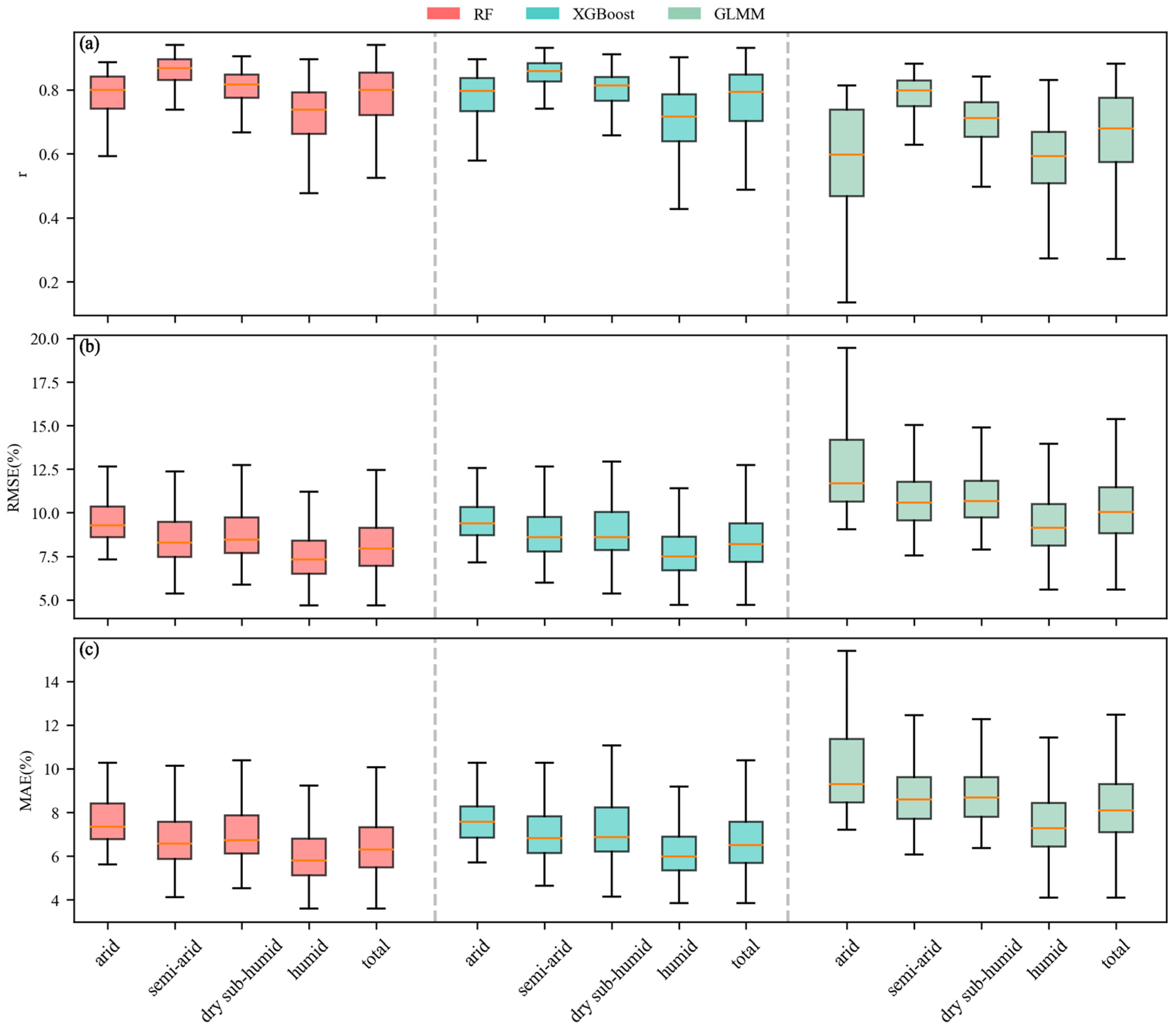
In order to further investigate the impact of climate zoning on RH estimation, box plots were used to present the comparison of estimation performance of different climate zones across various methods. The color variation in the box plots represented differences between methods. In this study, the primary focus of the analysis was to highlight the performance differences in each model across the various climate zones. In other words, the emphasis was placed on comparing variations within the same color category, which reflects how the performance of a single method differed from one zone to another. The metrics for this analysis were calculated based on 10% validation data each year from 2011 to 2020.
Based on the three statistical metrics, RF and XGBoost demonstrated excellent and comparable performance across all climate zones. The RMSE and MAE followed a consistent pattern across the different zones. Superior performance was observed in humid zones, while relatively lower accuracy was observed in arid zones. Specifically, the median value of RMSE in humid zones was approximately 7.4%, with a median value of MAE of about 5.8%, while in arid zones the median value of RMSE increased to approximately 9.3% and the median value of MAE was approximately 7.5% (Figure 4b,c). This indicates that the prediction error in arid zones was about 28–29% higher than in humid zones, reflecting significantly degraded model performance under arid conditions. Although RF and XGBoost showed highly similar overall trends, a detailed comparison of median values revealed nuanced differences. RF consistently outperformed XGBoost across all zones, with lower MAE and RMSE and marginally higher r. The advantage of RF was most pronounced in semi-arid zones, where its MAE and RMSE were 0.27% and 0.29% lower than those of XGBoost, respectively. Moreover, regarding the performance degradation from humid to arid zones, the median MAE of the RF model increased by 1.53%, while that of the XGBoost model increased by 1.61%. The mitigation was slightly more pronounced for RF than for XGBoost, suggesting that the RF may offer superior robustness in data-scarce arid zones. In contrast, the performance of the GLMM was markedly inferior, as indicated by the higher position and greater dispersion of whiskers in Figure 4. This was particularly evident in arid zones, which exhibited notably lower r values and substantial variability. Apart from r, the RMSE and MAE of the GLMM were significantly higher than those of the other two algorithms across all climate zones. However, it still maintained the pattern where RMSE and MAE were lowest in humid zones and highest in arid zones. These findings further illustrated that predictions in humid zones were more accurate than those in arid zones.
Figure 4.
The (a) r, (b) RMSE and (c) MAE of RF, XGBoost and GLMM methods in different climate zones. The line in the middle of the box (orange) represents the median of the data.
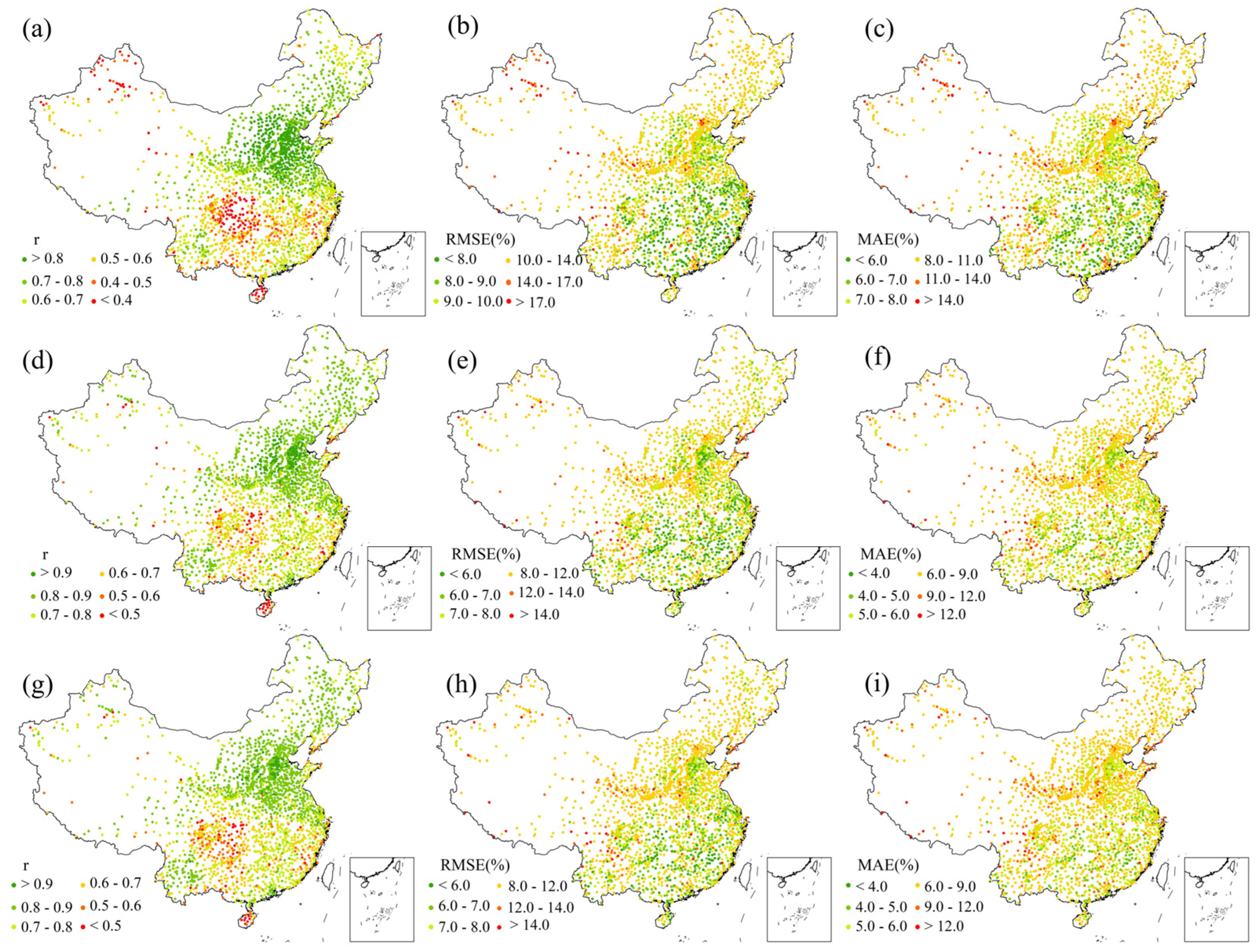
The specific spatial distribution of the models’ prediction accuracy is shown in Figure 5. In the northern areas, r values were generally higher across all methods (Figure 5a,d,g); however, the performance of the GLMM remained poor in these regions. The r values for the GLMM in these regions were only between 0.7 and 0.89. In RF and XGBoost, most of the meteorological stations in these areas had high r values, generally exceeding 0.7. This indicates that both RF and XGBoost models had a good fitting effect and effectively explained the variation in RH in these areas. On the contrary, for some meteorological stations in the northwest areas and the southern areas, r values were relatively low and exhibited greater instability. At many stations, the r values were lower than 0.7. Figure 5b,e,h show that RMSE values were relatively low at most meteorological stations. The eastern regions, particularly the southeastern areas, performed best. The RMSE values for the GLMM were mostly below 10%, whereas those of RF and XGBoost were predominantly below 8%. Although RMSE values in the high-altitude areas of the west were relatively high, they remained within an acceptable range overall. The spatial pattern of MAE (Figure 5c,f,i) was largely consistent with that of RMSE. The southeastern areas and the North China Plain maintained relatively low MAE values. The MAE values for the GLMM were mostly below 11%. In contrast, for most meteorological stations using RF and XGBoost, MAE values were below 9%, while values in the western regions were comparatively higher. Overall, most areas in China exhibited good RH estimation accuracy.
Figure 5.
The station accuracy metrics of RH: (a–c) represent the r, RMSE and MAE values obtained through the GLMM method; (d–f) represent the r, RMSE and MAE values obtained through the RF method; (g–i) represent the r, RMSE and MAE values obtained through the XGBoost method. All stations shown in the figure are statistically significant at p < 0.001.
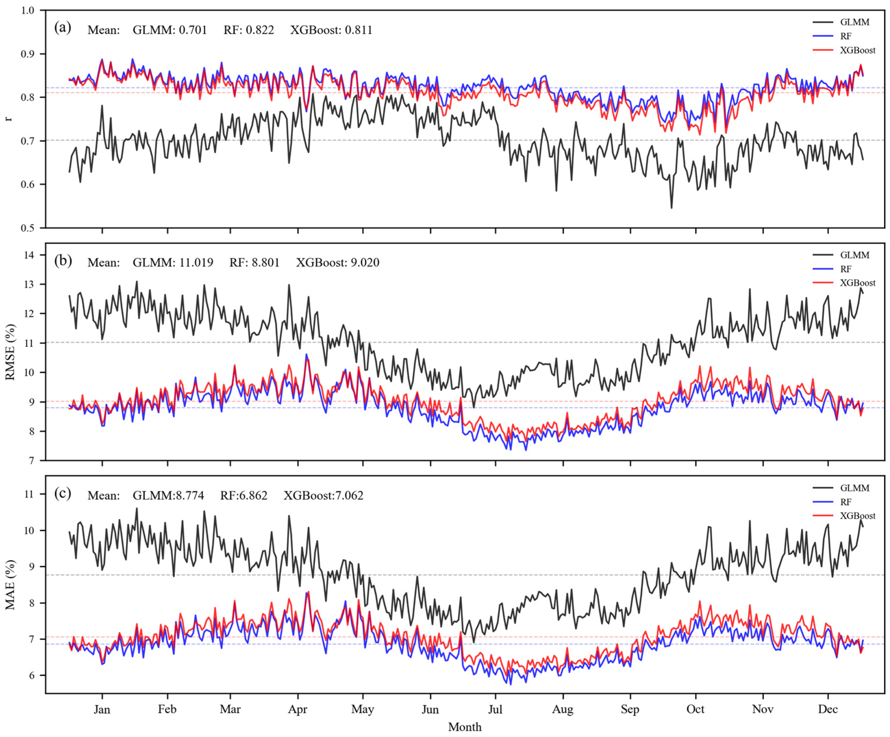
The performance of the models also varies with the seasons, as shown in Figure 6. Figure 6a shows that the daily r values of the GLMM was significantly lower than that of both the RF and XGBoost methods. Moreover, the r values of GLMM exhibited substantial fluctuations without a clear seasonal pattern. Its mean was 0.701, with a range of 0.55 to 0.82. In terms of the mean, the r of RF (r = 0.822) was slightly higher than that of XGBoost (r = 0.811). The r values of these two methods had a small range of variation and were highly consistent, ranging from 0.71 to 0.9. For both RF and XGBoost, r values remained around 0.84 during the first half of the year, began to decline from August, and gradually recovered by the end of the year. The RMSE values of all three methods exhibited distinct seasonal patterns, reaching their lowest values between July and September. This indicates that the models yielded lower errors during the summer. The daily RMSE values of the GLMM were higher than that of RF and XGBoost. The mean value for the GLMM was 11.019%, with a range of 8.8% to 13.1% (Figure 6b). In comparison, RF and XGBoost had mean values of 8.801% and 9.02%, respectively, with ranges of 7.5% to 10.7%. RF and XGBoost exhibited a unique seasonal pattern distinct from the GLMM. Their RMSE values increased significantly from March to April, peaking at approximately 10.7% in April. Subsequently, they gradually declined through the summer, slowly rose in autumn, and remained relatively stable during the winter months. The variation pattern of MAE values (Figure 6c) was highly consistent with that of RMSE values. This distinct seasonal pattern indicates that the prediction error was strongly influenced by seasonal changes. The lower RMSE and MAE values in summer suggested that the RH prediction error was smaller and the predictive performance was stronger during this season. Specifically, RH estimation was more accurate in summer.
Figure 6.
The daily (a) r, (b) RMSE and (c) MAE of RH from 2011 to 2020.
3.3. Spatial Distribution of RH at Different Spatial Scales
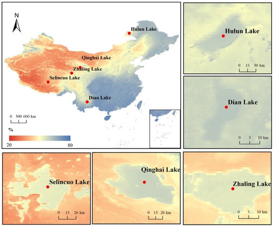
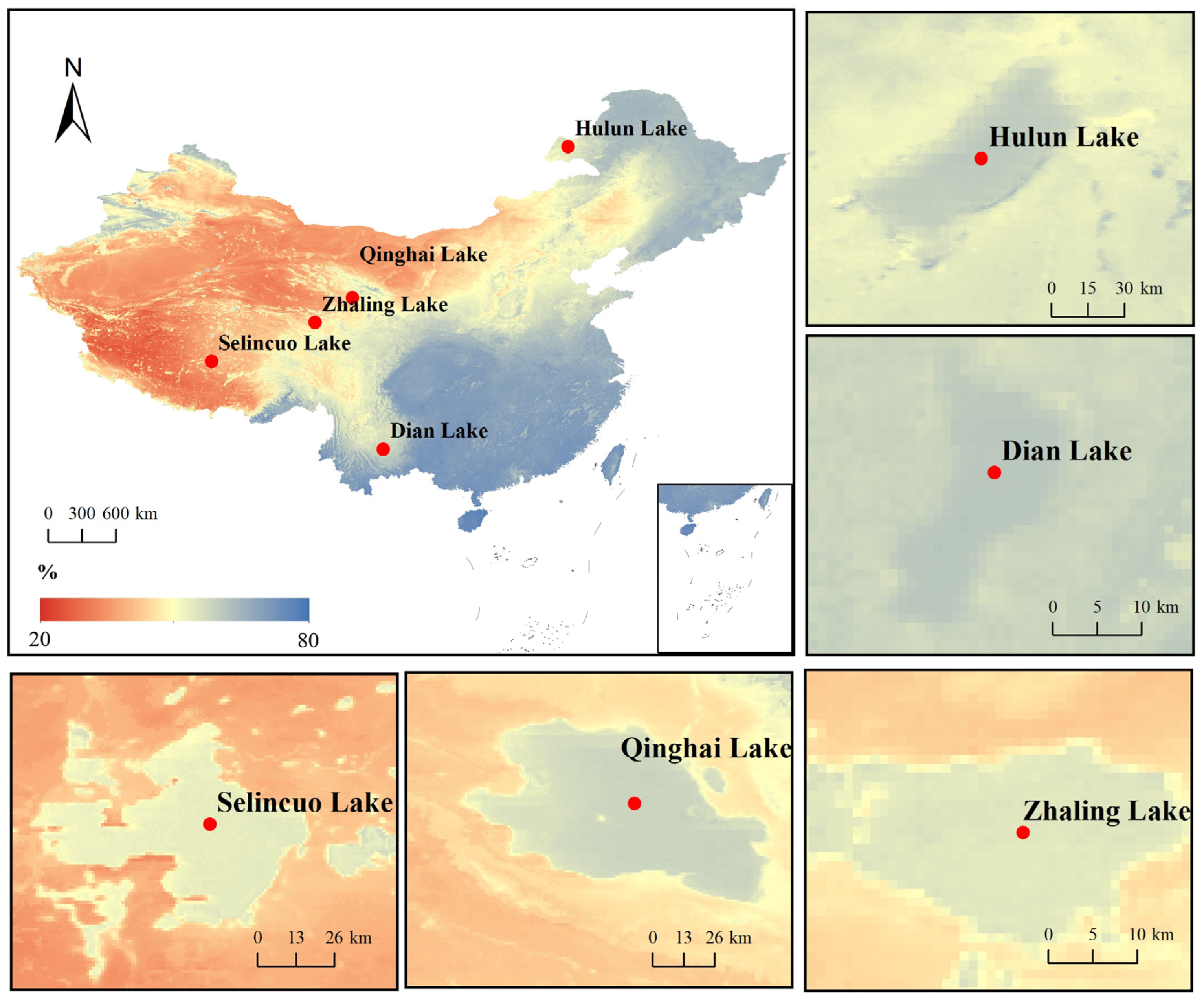
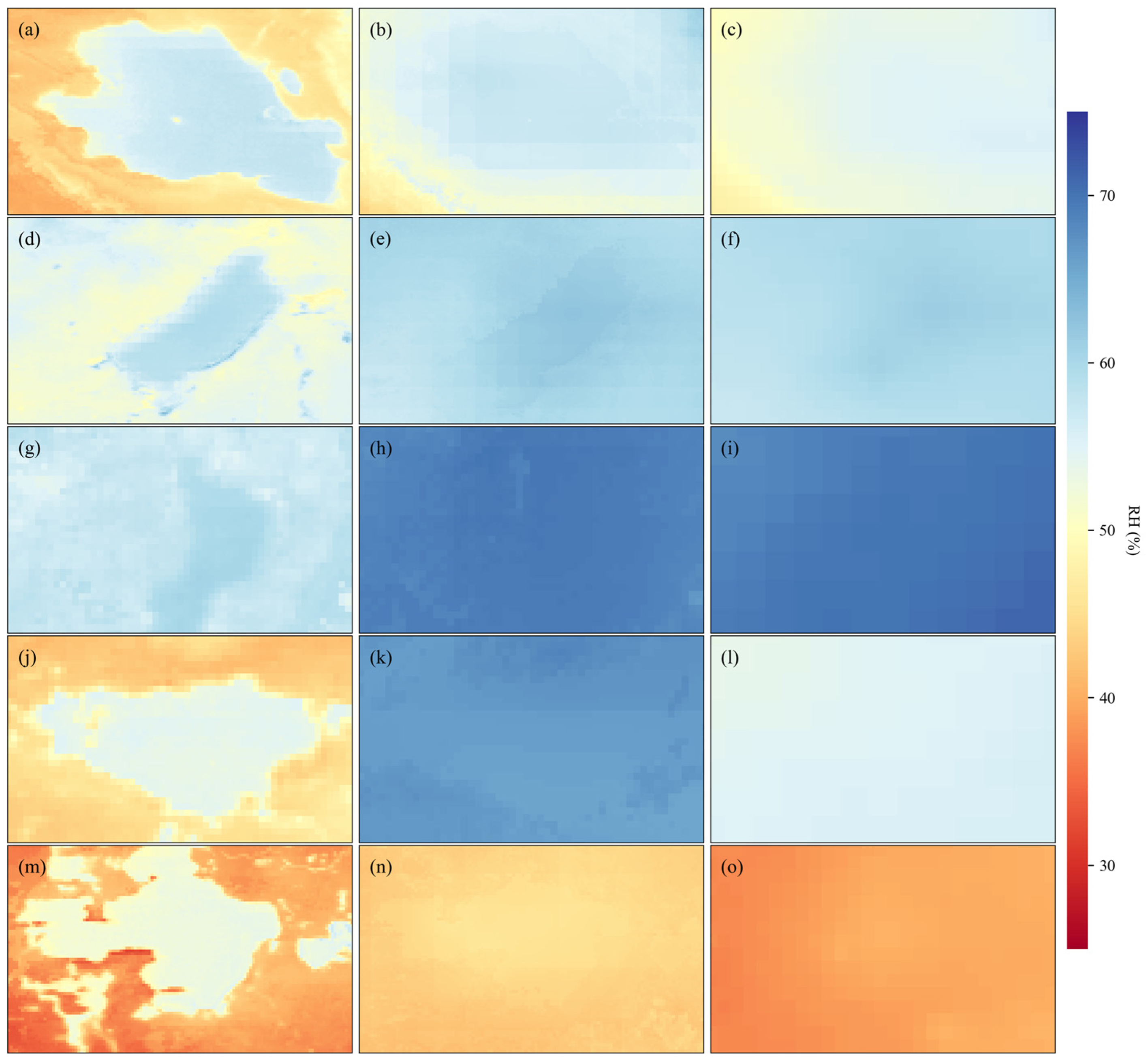
To analyze the distribution characteristics of the daily RH at different spatial scales, we used the RF method with the optimal performance to generate the daily RH distribution maps for two spatial scales (national and local) from 2011 to 2020 (Figure 7). At the national scale, the RH shows a spatial pattern of being higher in the southeast and lower in the northwest (Figure 7). To verify the reliability of the estimation results, we selected local areas with significant RH differences between water bodies and their surrounding environments for comparison. The results showed that the multiple lakes marked in the figure (Figure 7), including Hulun Lake, Dian Lake, Zhaling Lake, Qinghai Lake and Selincuo Lake, had significantly higher daily RH than the surrounding regions. This difference aligned with the physical characteristics of water bodies and objective facts, indicating that our estimation model accurately captured the high RH characteristics caused by large water bodies.
Figure 7.
Spatial Patterns of RH in Chinese Lakes from 2011–2020 based on the RF model.
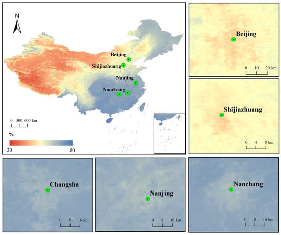
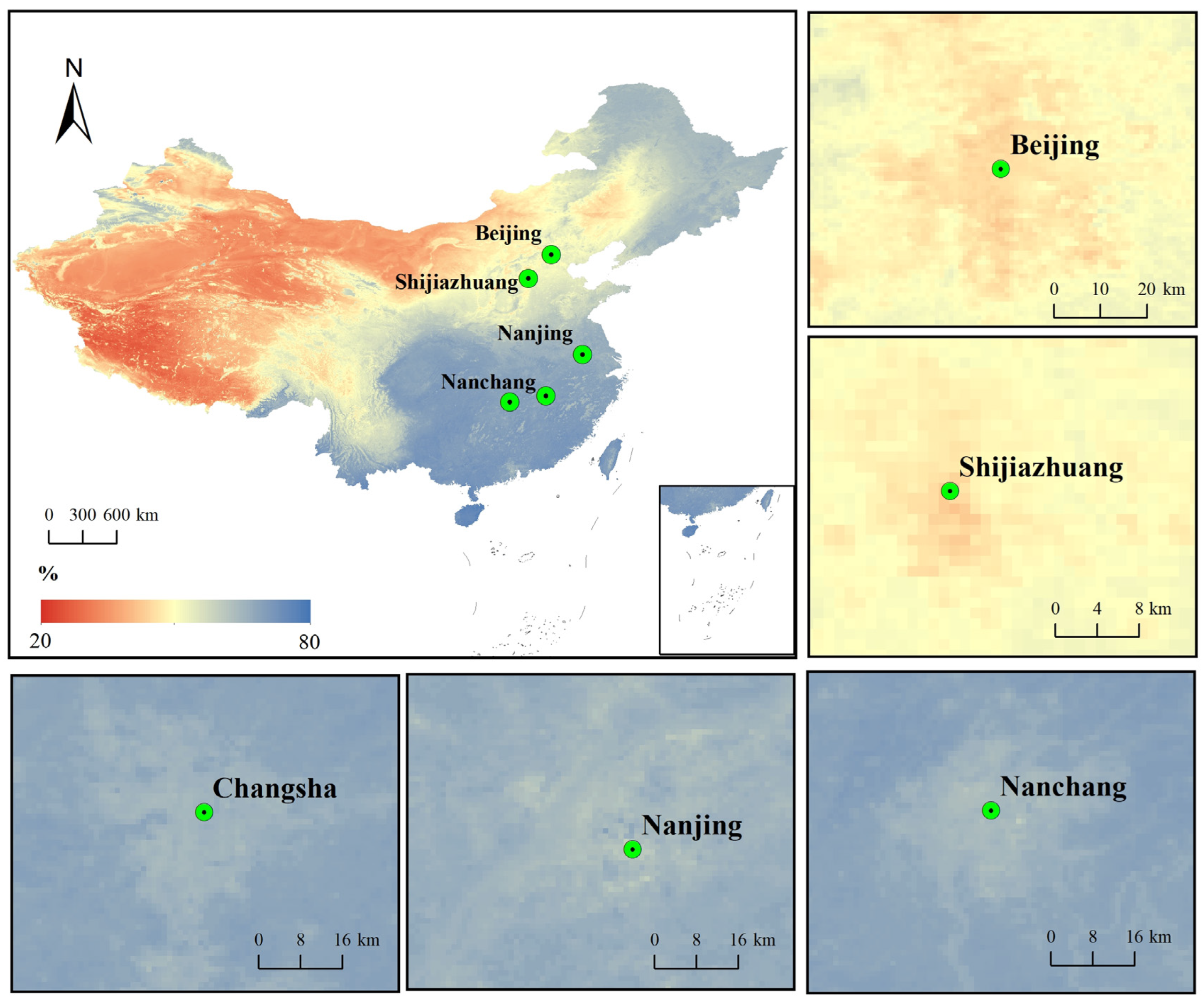
In addition to the RH differences between water bodies and the surrounding areas, we also examined the impact of urbanization on RH distribution by analyzing daily mean RH maps for several major cities, including Beijing, Shijiazhuang, Nanchang, Nanjing and Changsha (Figure 8). The results showed that the RH in urban centers was significantly lower than in the surrounding areas (Figure 8). This phenomenon was closely related to factors such as the large impervious surface area of the urban surface, the low vegetation coverage, and the release of human heat. This pattern conformed to the typical characteristics of the urban dry island (UDI) effect [61], further verifying the capturing ability of this model for the spatial differentiation pattern of RH under different surface types. These results confirmed that the RH estimation generated in this study was reliable and robust, making them suitable for further scientific analysis and application.
Figure 8.
Spatial Patterns of RH in Chinese Urban Centers from 2011–2020 based on the RF model.
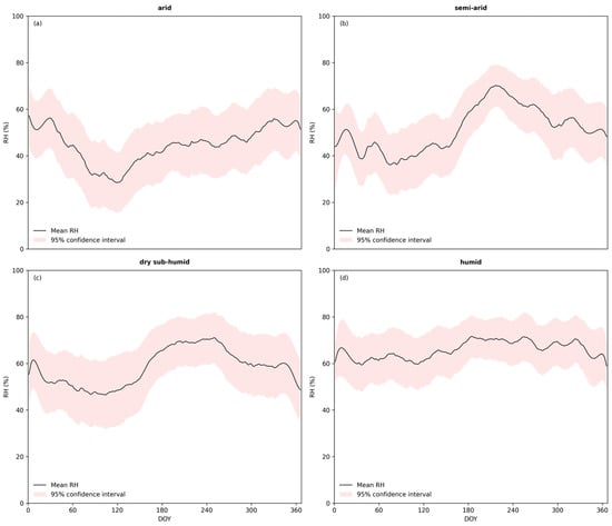
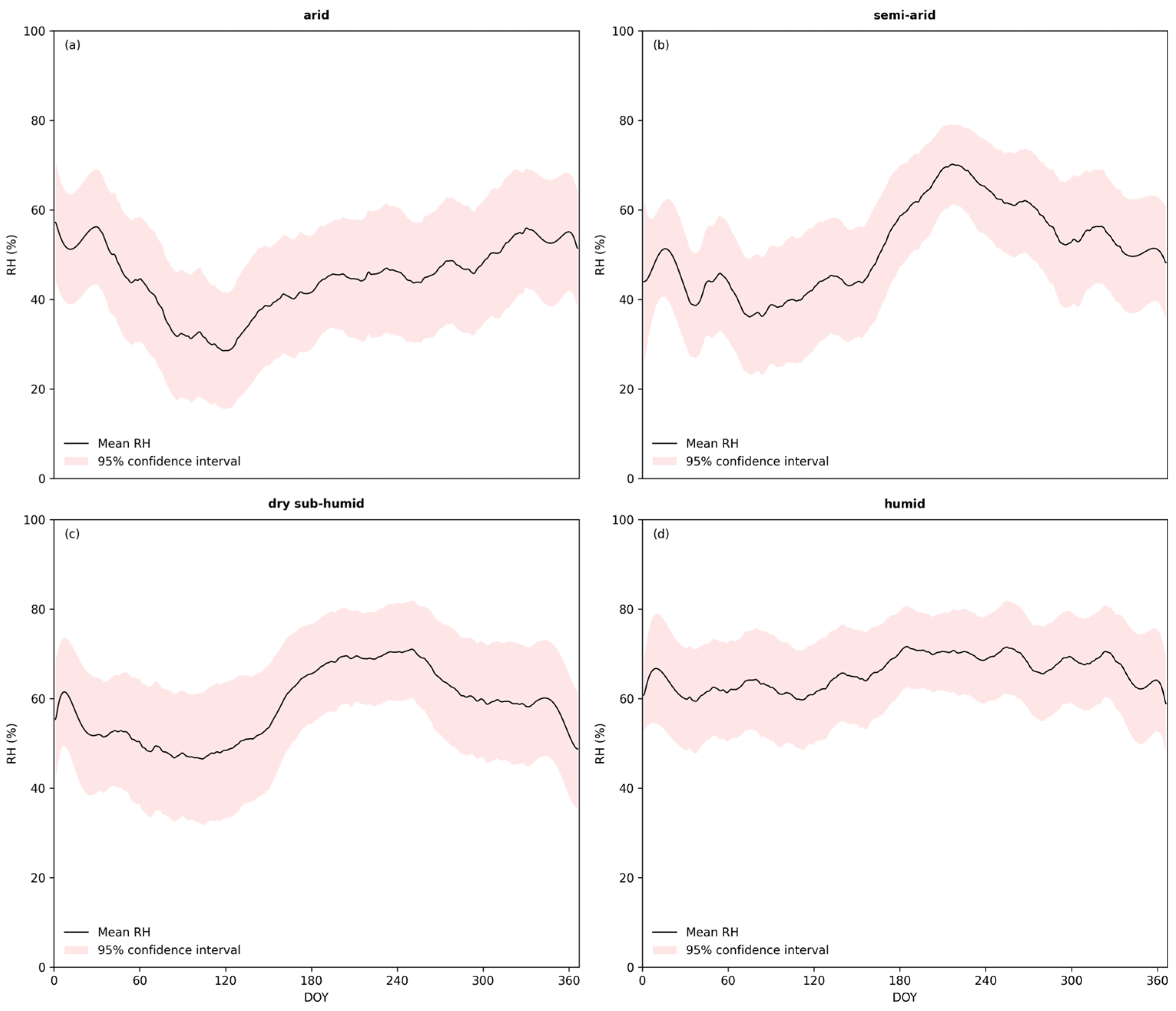
Figure 9 presents the spatiotemporal dynamics of daily mean RH across four climatic zones in China from 2011 to 2020, as simulated by the RF model. The findings indicate distinct regional disparities in daily mean RH. The humid zone recorded the highest mean value, approximately 66.3%, followed by the dry sub-humid zone at about 58.8%, the semi-arid zone at 50.8%, and the arid zone at 44.3%. Temporally, the humid zone exhibited relatively small intra-annual fluctuations in RH, whereas the other climatic zones displayed broadly similar seasonal cycles with spring troughs. However, the arid zone peaked in winter, while the semi-arid and dry sub-humid zones showed consistent patterns with summer peaks and winter troughs. This suggests significant differences in intra-annual RH variations across zones. Furthermore, except for the arid zone, all other climatic zones demonstrated narrower confidence intervals and lower uncertainty during summer, as clearly shown by the shaded areas in Figure 9. This indicates that the RF performed more accurately in estimating summer RH in these zones. In contrast, the arid zone did not show the same pattern, likely due to limited training data during summer, which restricted the model’s ability to capture sufficient information for reliable predictions.
Figure 9.
Daily mean relative humidity (RH) across climatic zones in China from 2011 to 2020, based on the RF model. The four zones are: (a) arid, (b) semi-arid, (c) dry sub-humid and (d) humid. Shaded areas represent 95% confidence intervals.
4. Discussion
4.1. Comparison with Previous Studies and Other Datasets
Previous studies have mainly estimated RH using interpolation [29], machine learning [31], or calculations based on saturation vapor pressure () and actual vapor pressure [25], as summarized in Table 4. However, Kloog et al. [43] incorporated the LMM to achieve high precision temperature estimates, offering a new perspective for estimating time-sensitive meteorological variables. This inspired our hypothesis that a GLMM could be developed using temporal grouping of the data to more effectively capture the temporal variation in the relationship between and RH [16]. Although the GLMM underperformed relative to the machine learning approaches in this study, its estimation accuracy (RMSE = 10.84–11.54%) was comparable to that reported by Li et al. [23] (RMSE = 11.06%). Therefore, estimating RH using GLMMs may also serve as a viable alternative. Relying solely on the fixed model structure of GLMMs makes it difficult to flexibly capture the complex relationship between and RH over time, thereby limiting its final performance [62]. Ensemble methods excel at capturing such complex nonlinear relationships within data. As advanced ensemble techniques, RF and XGBoost integrate multiple decision trees [63]. Through recursive partitioning of the feature space, decision trees can fit intricate nonlinear mappings between input features and the target variable, and ensemble strategies further amplify this capability [64]. Feature interactions play a crucial role in RH estimation. Tree-based models automatically detect and leverage these interactions by partitioning different combinations of features across various trees. In contrast, the GLMM cannot fully capture the higher-order or nonlinear interactions present in the data [65]. Moreover, GLMMs are excessively sensitive to outliers, which can directly distort parameter estimates and significantly compromise model fit [66]. In RF, the influence of outliers on any single tree is diluted by the aggregated results from the multitude of trees, rendering RF robust to outliers [67]. This inherent robustness also constitutes a key reason why RF outperformed XGBoost in our analysis—a finding that stands in contrast to the results reported by Park et al. [31] for the Japan-Korea region. This discrepancy may be attributed to China’s greater climatic diversity, where unique geographical characteristics likely demand models with higher complexity and stronger robustness [68]. Both RF and XGBoost demonstrated consistent spatiotemporal performance patterns, with model accuracy peaking during summer months and showing lower errors in southern regions. These findings aligned with the observations by Zhang et al. [33] and Zhang et al. [69], further validating the reliability of our results. Moreover, we extended the analysis to examine performance variations across different climate zones, providing a more granular understanding of model behavior. In terms of spatial patterns of estimated RH, our results showed high consistency with those of Zhang et al. [33] and Zhang et al. [69]. However, our study achieves superior temporal and spatial resolution compared to these earlier works.
Table 4.
Summary of the RH estimation in previous studies.
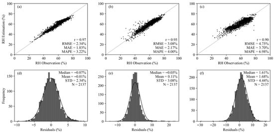
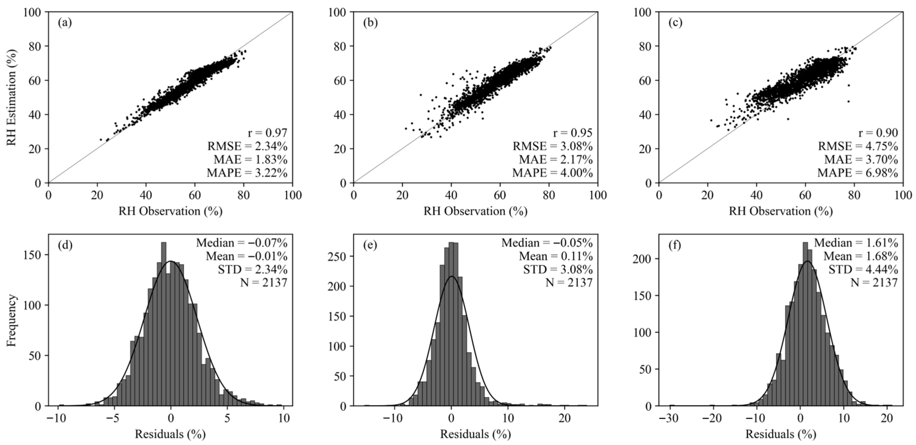
Comparison with existing datasets further demonstrated the advantage of this study. The CDMet dataset provides nationwide meteorological coverage, granting it irreplaceable value for large-scale macroscopic analyses. However, its relatively low estimation accuracy (r = 0.90, RMSE = 4.75%, mean absolute percentage error (MAPE) = 6.98%) (Figure 10c,f) and systematic overestimation with high volatility in residual analysis indicated that it is more suitable for studies where absolute precision is not critical. The ChinaMet dataset, while significantly outperforming CDMet (r = 0.95, RMSE = 3.08%, MAPE = 4.00%) (Figure 10b,e), still fell short of our proposed approach. Its primary limitation likely stems from excessive reliance on low-resolution reanalysis data as input. Biases inherent in reanalysis products may be directly propagated to the estimated RH, constraining its ability to capture localized fine-scale variations. In contrast, the RF model developed in this study achieved optimal performance across all evaluation metrics (r = 0.97, RMSE = 2.34%, MAPE = 3.22%) (Figure 10a,d), with a residual distribution that was both centralized and unbiased.
Figure 10.
Scatterplot and frequency histogram of comparison with the production dataset of others: (a) Scatterplot of this study. (b) Scatterplot of the ChinaMet dataset. (c) Scatterplot of the CDMet dataset. (d) Frequency histogram of this study. (e) Frequency histogram of the ChinaMet dataset. (f) Frequency histogram of the CDMet dataset.
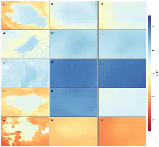
To further highlight the model’s capability in reproducing fine-scale spatial patterns, Figure 11 presents a localized comparison over five representative lake regions: Qinghai Lake, Hulun Lake, Dian Lake, Zhaling Lake and Selincuo Lake. The spatial details clearly demonstrate that our RF-based model accurately captured the sharp RH gradients at land-water interfaces. In contrast, both the CDMet and ChinaMet datasets exhibited evident spatial over-smoothing, failing to resolve these localized features. This visual evidence reinforces that our approach successfully overcame the limitations associated with low-resolution reanalysis inputs, providing superior performance not only in statistical metrics but also in spatial fidelity.
Figure 11.
Spatial patterns of local RH around five major lakes in China derived from this study (left column), ChinaMet (middle column) and CDMet (right column) for five Chinese lakes: Qinghai Lake (a–c), Hulun Lake (d–f), Dian Lake (g–i), Zhaling Lake (j–l) and Selincuo Lake (m–o).
4.2. Uncertainties and Limitations
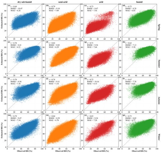
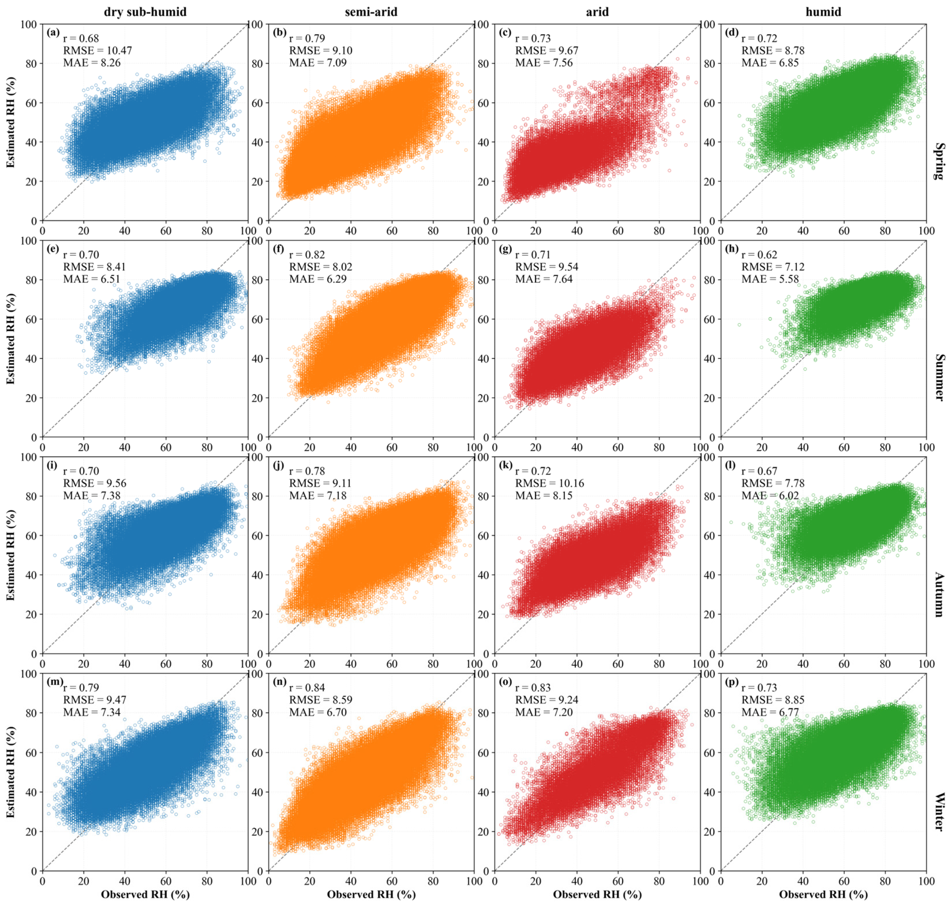
There are also many uncertainties in the process of estimating RH, and it is necessary to discuss the sources of these uncertainties. In theory, there is a certain relationship among , and RH [16]. Hence, using near-surface and data from satellite data to estimate RH has become a viable method. During the estimation process, the validity of RH is affected by the accuracy of and . In this study, both and were obtained through processing with MOD07 product. For variables such as and , the ERA5 reanalysis data might be a more popular choice due to its global coverage and absence of data gaps [3,18,31,70,71]. However, as the best alternative data source, MOD07 has a significantly higher spatial resolution than ERA5 [35]. Hydrological phenomena exhibit similarities. The geographical conditions within the same climate zone are relatively similar, and the underlying surface conditions are also relatively consistent [72]. According to a study by Zhu et al. [34], each climate zone showed different levels of accuracy for . The extracted by the ALR method was less accurate in semi-arid and dry sub-humid zones. The accuracy of extracting from the MOD07 product varies not only by climate zone but also by season. In addition to the description of the accuracy of the correction method in each season, Zhu et al. [34] also presented the relationship between the original accuracy of extracted by the ALR method and the seasons. The results showed that the accuracy of is low in spring and high in summer. Zhang et al. [73] showed that the extracted by the ALR method had the lowest accuracy in summer and the highest in winter. Moreover, the accuracy of is affected by altitude, with greater errors occurring at high altitudes. A synthesis of these studies, considering the geographical distribution in Figure 1, suggests that the MOD07 product achieves higher accuracy in humid zones. However, from the perspective of seasons, there is a conflict in the accuracy of the two dependent variables. As can be seen from Figure 3, the importance of is much lower than that of . Therefore, our analysis primarily considered the seasonal accuracy pattern of . As expected, Figure 6 shows that the overall area has low errors in summer. Figure 12 reveals that except in the arid zone, the winter errors (RMSE = 9.24%, MAE = 7.20%) are lower than those in summer (RMSE = 9.54%, MAE = 7.64%), and in the other three climate zones, the summer errors are the lowest. From the perspective of the climate zone, Figure 4 shows that the error in the humid zone is the lowest. When comparing with the same season, as shown in Figure 12, except for winter, the error in the semi-arid zone (RMSE = 8.59%, MAE = 6.70%) is slightly lower than that in the humid zone (RMSE = 8.85%, MAE = 6.77%), and in all other seasons, the error in the humid zone is the lowest. These errors in estimating RH are broadly consistent with the error assessment results obtained from the and values processed by the MOD07 product.
Figure 12.
Cross-seasonal scatter plot of RH in different climate zones. Each row represents a season: (a–d) Spring, (e–h) Summer, (i–l) Autumn and (m–p) Winter. Each column represents a climatic zone: dry sub-humid (a,e,i,m), semi-arid (b,f,j,n), arid (c,g,k,o) and humid (d,h,l,p). Different colors represent different climatic zones.
Specifically, as observed by Zhu et al. [34], the input MOD07 data itself contains errors, which will have an impact on the subsequent correction methods. Machine learning models learn the complex mapping relationships between these data and the ground truth [74,75,76]. If there are systematic biases in the input data, the models are likely to learn and amplify these biases, which will introduce greater uncertainty into the estimation of RH [77].
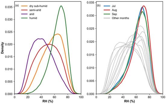
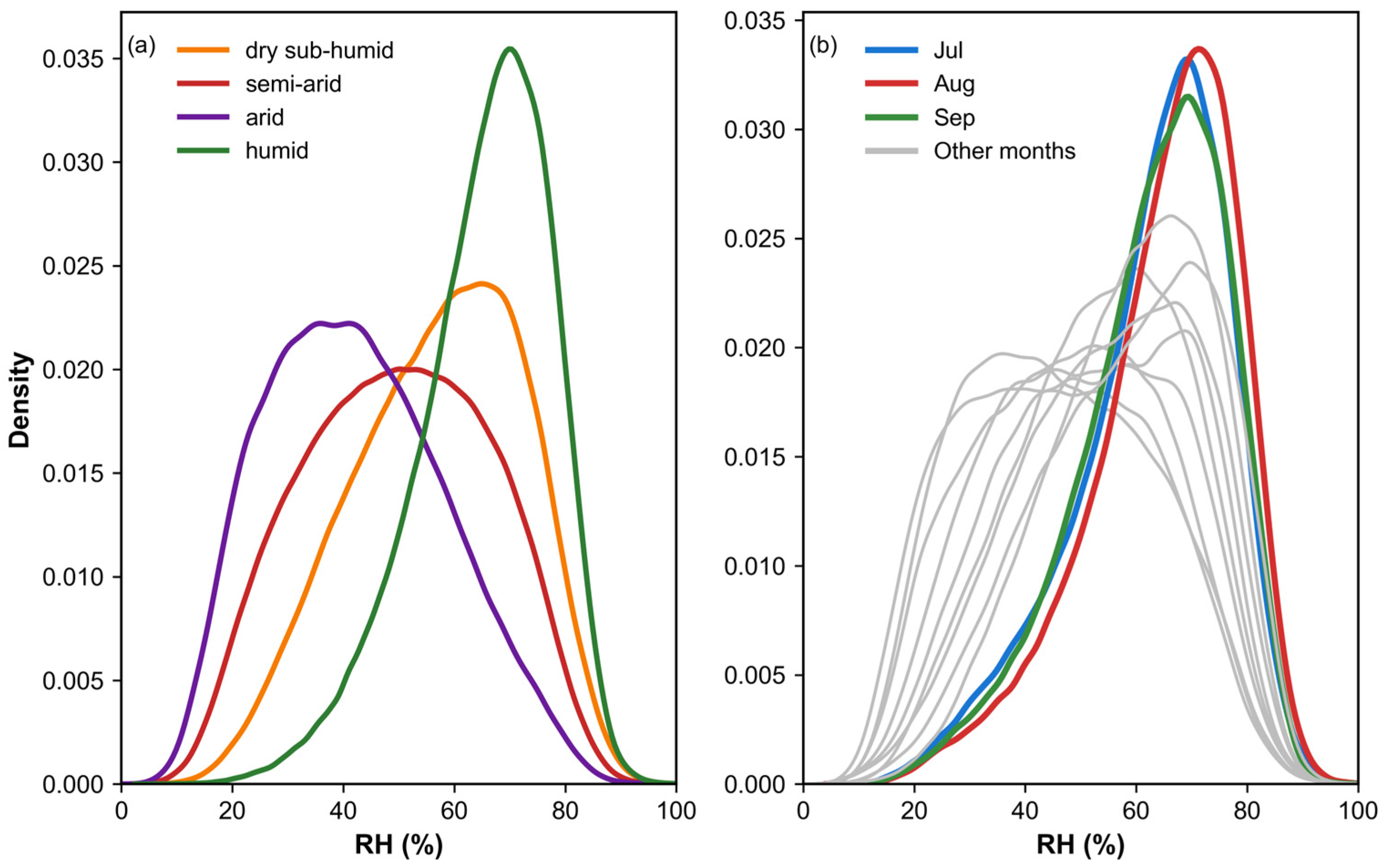
There are significant regional differences in the model performance for estimating RH. Our findings highlighted minimal errors in humid zones, which could be attributed to the high accuracy of MOD07 product, the greater number of meteorological stations and the greater abundance of available training data. However, as shown in Figure 4 and Figure 5, while the model’s error was lowest in humid zones, the r was, conversely, smaller than in other climate zones. Understanding the reason for this phenomenon is crucial for analyzing the geographical variations in performance. This apparent contradiction can be explained by the distribution of RH itself. Combined with Figure 13a, the distribution characteristics reveal that RH in humid zones was highly concentrated within a narrow range of 80% to 100%, exhibiting a sharp, high-peaked density distribution and extremely limited variability. The r measures the strength of the linear relationship between estimation and observation of RH. Typically, when the target variable’s data distribution is concentrated and its variability is low, the consistency in fluctuation trends between predicted and observed values is difficult to reflect, often resulting in a low calculated r [78]. Therefore, the pressing issue that needs to be addressed is enabling the model to capture the variability across various climate zones. However, the current r is within an acceptable range, and multiple independent statistical metrics have confirmed that the model demonstrates good overall performance, with residual analysis also showing no obvious systematic bias. For other climate zones, arid, semi-arid and dry sub-humid zones exhibit similar RH distribution characteristics. In contrast, the model’s estimation accuracy in arid zones is significantly lower, which may be attributed to the sparse meteorological stations in these zones and a severe lack of data available for training and validation [79,80]. Thus, the model faces a dual challenge from sample imbalance: capturing subtle variability in data-rich, low-variance humid zones, and overcoming outright data scarcity in arid zones. Beyond these spatial constraints, temporal dynamics also significantly influence model performance. Our evaluation of the model’s daily performance confirmed significant seasonal variations, with errors substantially lower from July to September than in other periods. As shown in Figure 13b, the RH distribution during this period was more concentrated than in other months, suggesting that the inherent stability of the target variable itself might have contributed to its relatively low RMSE. Furthermore, the MOD07 product used in this study is also more accurate during the summer, providing better input data for the model.
Figure 13.
The density of RH measurement values in (a) different climate zones and (b) months.
Despite the model’s overall strong performance in this study, it still has some shortcomings. Therefore, we propose the following recommendations for future research. Firstly, the MOD07 product itself presents certain limitations. The and derived from it are subject to accuracy constraints. As our analysis heavily relies on the accuracy of these two variables, we recognize that future work could explore alternative methods to improve the reliability of and , which, in turn, would enhance the accuracy of RH estimation. Secondly, the modeling was refined to address specific conditions within each climate zone. This refinement not only enabled more accurate estimation of local RH but also provided deeper insights into how various variables exert their influence across different climate zones and seasons, ultimately yielding more detailed conclusions. It is important to note, however, that the potential of this climate-specific modeling is constrained by underlying sample imbalance. Future efforts to fully realize this approach would need to integrate advanced techniques—such as transfer learning or data augmentation—to mitigate data scarcity and ensure balanced learning across diverse climates.
In summary, this study successfully estimated spatially continuous, high resolution RH data. This achievement not only provides a reliable data foundation for relevant fields but also contributes to advancing future research by enhancing model robustness and applicability under diverse geographical and climatic conditions.
5. Conclusions
In this study, we successfully constructed a high spatiotemporal resolution RH dataset for China using observational data and remote sensing data. We identified , , DEM, NDVI, DOY and AI as independent variables. The performance of multiple models was then evaluated using a set of commonly used statistical metrics. Through comparative analysis, RF demonstrated superior performance among multiple models, with its robustness validated. The results further indicated its strong ability to reduce prediction errors. We further quantified the contribution of each independent variable, which revealed that , AI and DOY are the main contributing factors for RH estimation. Notably, AI, a quantitative measure of a region’s climatic aridity, exhibited high importance in both the RF and XGBoost models. The variable importance analysis further highlighted variations in model performance across different climate zones. Specifically, prediction errors were lower in humid zones, whereas highly accurate RH estimations in arid zones proved relatively more challenging. In addition to spatial heterogeneity, we hypothesized that temporal factors would significantly influence RH estimation. Therefore, we further investigated the model’s daily performance. The results indicated that the estimation performance of RH exhibits pronounced seasonality, with the model achieving the lowest errors during summer. This finding further underscores the necessity incorporating temporal variables for reliable RH estimation. Overall, this study provided valuable insights and a robust methodology for generating high-resolution RH datasets, applicable across diverse climates, and explicitly identified limitations pertaining to input data quality and model performance to guide future research.
Author Contributions
Conceptualization, Y.Y. and W.Z.; methodology, Y.Y. and W.Z.; software, L.W.; validation, Y.Y., L.W., H.L. and W.Z.; formal analysis, L.W.; investigation, Y.Y. and H.L.; resources, Y.Y. and L.W.; data curation, W.Z.; writing—original draft preparation, Y.Y.; writing—review and editing, Y.Y., L.W., H.L. and W.Z.; visualization, Y.Y.; supervision, W.Z.; project administration, W.Z.; funding acquisition, W.Z. All authors have read and agreed to the published version of the manuscript.
Funding
This study was supported by the Science and Technology Department of Qinghai Province (2024-SF-A6) and National Natural Science Foundation of China (32471972).
Data Availability Statement
The original contributions presented in this study are included in the article. Further inquiries can be directed to the corresponding author.
Acknowledgments
This research was supported by the following data sources: station data were obtained from the China Meteorological Data Service Center (http://data.cma.cn, accessed on 13 March 2025), and MODIS products were courtesy of the NASA EOSDIS Land Processes Distributed Active Archive Center. We also acknowledge the use of geospatial data from the U.S. Geological Survey’s Earth Resources Observation and Science Center. Furthermore, we are grateful to the providers of the meteorological observations and the global aridity index dataset, namely the China Meteorological Data Service Center and the Consortium for Spatial Information of the Consultative Group for International Agricultural Research. The authors would like to extend their sincere gratitude to the handling editor and the anonymous reviewers. Their constructive comments and insightful suggestions were invaluable and greatly improved the quality of this manuscript.
Conflicts of Interest
The authors declare no conflicts of interest.
References
- Li, Z.; Yan, Z.; Zhu, Y.; Freychet, N.; Tett, S. Homogenized Daily Relative Humidity Series in China during 1960–2017. Adv. Atmos. Sci. 2020, 37, 318–327. [Google Scholar] [CrossRef] [Scilit]
- Randall, D.A.; Wood, R.A.; Bony, S.; Colman, R.; Fichefet, T.; Fyfe, J.; Kattsov, V.; Pitman, A.; Shukla, J.; Srinivasan, J.; et al. Climate Models and Their Evaluation. In Climate Change 2007: The Physical Science Basis. Contribution of Working Group I to the Fourth Assessment Report of the IPCC (FAR); Qin, D., Manning, M., Chen, Z., Marquis, M., Averyt, K.B., Tignor, M., Miller, H.L., Eds.; Cambridge University Press: Cambridge, UK, 2007; pp. 589–662. [Google Scholar]
- Viggiano, M.; Geraldi, E.; Cimini, D.; Di Paola, F.; Gallucci, D.; Gentile, S.; Larosa, S.; Nilo, S.T.; Ricciardelli, E.; Romano, F. The role of temporal resolution of meteorological inputs from reanalysis data in estimating air humidity for modelling applications. Agric. For. Meteorol. 2021, 311, 108672. [Google Scholar] [CrossRef] [Scilit]
- Farahmand, A.; AghaKouchak, A.; Teixeira, J. A Vantage from Space Can Detect Earlier Drought Onset: An Approach Using Relative Humidity. Sci. Rep. 2015, 5, 8553. [Google Scholar] [CrossRef] [Scilit] [PubMed]
- Wang, B.; Shen, S.; Lao, W.I.; Kan, L.W.; Chan, I.T.; He, C.B.; He, J.Q.; Wong, U.H.; Lao, E.P.L.; Smith, R.D. Associations of ambient temperature and relative humidity with hospital admissions in macau, China using time series analysis. Sci. Rep. 2025, 15, 25968. [Google Scholar] [CrossRef] [Scilit] [PubMed]
- Colston, J.M.; Ahmed, T.; Mahopo, C.; Kang, G.; Kosek, M.; de Sousa Junior, F.; Shrestha, P.S.; Svensen, E.; Turab, A.; Zaitchik, B.; et al. Evaluating meteorological data from weather stations, and from satellites and global models for a multi-site epidemiological study. Environ. Res. 2018, 165, 91–109. [Google Scholar] [CrossRef] [Scilit] [PubMed]
- Santos-Vega, M.; Martinez, P.P.; Vaishnav, K.G.; Kohli, V.; Desai, V.; Bouma, M.J.; Pascual, M. The neglected role of relative humidity in the interannual variability of urban malaria in Indian cities. Nat. Commun. 2022, 13, 533. [Google Scholar] [CrossRef] [Scilit]
- Jain, P.; Castellanos-Acuna, D.; Coogan, S.C.P.; Abatzoglou, J.T.; Flannigan, M.D. Observed increases in extreme fire weather driven by atmospheric humidity and temperature. Nat. Clim. Change 2021, 12, 63–70. [Google Scholar] [CrossRef] [Scilit]
- Matteo, A.; Garnés-Morales, G.; Moreno, A.; Ribeiro, A.F.S.; Azorin-Molina, C.; Bedia, J.; Di Giuseppe, F.; Dunn, R.J.H.; Herrera, S.; Provenzale, A.; et al. Challenges in assessing Fire Weather changes in a warming climate. npj Clim. Atmos. Sci. 2025, 8, 284. [Google Scholar] [CrossRef] [Scilit]
- Douville, H.; Qasmi, S.; Ribes, A.; Bock, O. Global warming at near-constant tropospheric relative humidity is supported by observations. Commun. Earth Environ. 2022, 3, 237. [Google Scholar] [CrossRef] [Scilit]
- Peixóto, J.P.; Oort, A.H. The Atmospheric Branch of the Hydrological Cycle and Climate. In Variations in the Global Water Budget; Street-Perrott, A., Beran, M., Ratcliffe, R., Eds.; Springer: Dordrecht, The Netherlands, 1983; pp. 5–65. [Google Scholar]
- Trenberth, K.E. Conceptual Framework for Changes of Extremes of the Hydrological Cycle with Climate Change. Clim. Change 1999, 42, 327–339. [Google Scholar] [CrossRef] [Scilit]
- Penman, H.L. Natural evaporation from open water, bare soil and grass. Proc. R. Soc. Lond. A 1948, 193, 120–145. [Google Scholar] [CrossRef] [Scilit]
- Easterbrook, D.J. Greenhouse Gases. In Evidence-Based Climate Science; Elsevier: Amsterdam, The Netherlands, 2016; pp. 163–173. [Google Scholar]
- Mills, G.; Draper, C. The Atmospheric Water Balance over the Semiarid Murray–Darling River Basin. J. Hydrometeorol. 2008, 9, 521–534. [Google Scholar] [CrossRef] [Scilit]
- Allan, R.; Pereira, L.; Smith, M. Crop Evapotranspiration-Guidelines for Computing Crop Water Requirements; FAO Irrigation and Drainage Paper No. 56; FAO: Rome, Italy, 1998. [Google Scholar]
- Yin, C.; Wang, K.; Li, R.; Zhang, Z. Homogenization of the Observed Surface Relative Humidity From 1959 to 2020 in China. J. Geophys. Res. Atmos. 2025, 130, e2024JD042644. [Google Scholar] [CrossRef] [Scilit]
- Shi, F.; Xin, J.; Yang, L.; Cong, Z.; Liu, R.; Ma, Y.; Wang, Y.; Lu, X.; Zhao, L. The first validation of the precipitable water vapor of multisensor satellites over the typical regions in China. Remote Sens. Environ. 2018, 206, 107–122. [Google Scholar] [CrossRef] [Scilit]
- Zhan, C.; Jiang, W.; Zheng, Y.; Lu, J.; Zhang, Q. A data-driven study of active meteorological stations and the factors motivating their establishment. Sustain. Energy Technol. Assess. 2023, 57, 103147. [Google Scholar] [CrossRef] [Scilit]
- Wen, Q.; Liu, K.; Li, Y.; Li, X.; Song, W. Climatic characteristics and meteorology-sensitivity of surface solar radiation in reanalysis products compared to observations and satellite data over China. Atmos. Environ. 2024, 334, 120713. [Google Scholar] [CrossRef] [Scilit]
- Guo, J.; Zhang, J.; Yang, K.; Liao, H.; Zhang, S.; Huang, K.; Lv, Y.; Shao, J.; Yu, T.; Tong, B.; et al. Investigation of near-global daytime boundary layer height using high-resolution radiosondes: First results and comparison with ERA5, MERRA-2, JRA-55, and NCEP-2 reanalyses. Atmos. Chem. Phys. 2021, 21, 17079–17097. [Google Scholar] [CrossRef] [Scilit]
- Krähenmann, S.; Walter, A.; Brienen, S.; Imbery, F.; Matzarakis, A. High-resolution grids of hourly meteorological variables for Germany. Theor. Appl. Climatol. 2016, 131, 899–926. [Google Scholar] [CrossRef] [Scilit]
- Li, T.; Zheng, X.; Dai, Y.; Yang, C.; Chen, Z.; Zhang, S.; Wu, G.; Wang, Z.; Huang, C.; Shen, Y.; et al. Mapping near-surface air temperature, pressure, relative humidity and wind speed over Mainland China with high spatiotemporal resolution. Adv. Atmos. Sci. 2014, 31, 1127–1135. [Google Scholar] [CrossRef] [Scilit]
- Hao, J.; Lu, E. The Consistent Variations of Precipitable Water and Surface Water Vapor Pressure at Interannual and Long-Term Scales: An Examination Using Reanalysis. Atmosphere 2022, 13, 1350. [Google Scholar] [CrossRef] [Scilit]
- Liao, Q.-Y.; Leng, P.; Li, Z.-L.; Ren, C.; Sun, Y.-Y.; Gao, M.-F.; Duan, S.-B.; Shang, G.-F. A Method for Deriving Relative Humidity From MODIS Data Under All-Sky Conditions. IEEE Trans. Geosci. Electron. 2021, 59, 8992–9006. [Google Scholar] [CrossRef] [Scilit]
- Kloog, I.; Chudnovsky, A.; Koutrakis, P.; Schwartz, J. Temporal and spatial assessments of minimum air temperature using satellite surface temperature measurements in Massachusetts, USA. Sci. Total Environ. 2012, 432, 85–92. [Google Scholar] [CrossRef] [Scilit]
- Nikolaou, N.; Dallavalle, M.; Stafoggia, M.; Bouwer, L.M.; Peters, A.; Chen, K.; Wolf, K.; Schneider, A. High-resolution spatiotemporal modeling of daily near-surface air temperature in Germany over the period 2000–2020. Environ. Res. 2023, 219, 115062. [Google Scholar] [CrossRef] [Scilit] [PubMed]
- Yao, A.Y.M. A Statistical Model for the Surface Relative Humidity. J. Appl. Meteorol. 1974, 13, 17–21. [Google Scholar] [CrossRef] [Scilit]
- Li, L.; Zha, Y. Mapping relative humidity, average and extreme temperature in hot summer over China. Sci. Total Environ. 2018, 615, 875–881. [Google Scholar] [CrossRef] [Scilit] [PubMed]
- Nikolaou, N.; Bouwer, L.M.; Dallavalle, M.; Valizadeh, M.; Stafoggia, M.; Peters, A.; Wolf, K.; Schneider, A. Improved daily estimates of relative humidity at high resolution across Germany: A random forest approach. Environ. Res. 2023, 238, 117173. [Google Scholar] [CrossRef] [Scilit]
- Park, H.; Lee, J.; Yoo, C.; Sim, S.; Im, J. Estimation of Spatially Continuous Near-Surface Relative Humidity Over Japan and South Korea. IEEE J. Sel. Top. Appl. Earth Obs. Remote Sens. 2021, 14, 8614–8626. [Google Scholar] [CrossRef] [Scilit]
- Zhang, L.; Li, X.; Zheng, D.; Zhang, K.; Ma, Q.; Zhao, Y.; Ge, Y. Merging multiple satellite-based precipitation products and gauge observations using a novel double machine learning approach. J. Hydrol. 2021, 594, 125969. [Google Scholar] [CrossRef] [Scilit]
- Zhang, J.; Liu, B.; Ren, S.; Han, W.; Ding, Y.; Peng, S. A 4 km daily gridded meteorological dataset for China from 2000 to 2020. Sci. Data 2024, 11, 1230. [Google Scholar] [CrossRef] [Scilit]
- Zhu, W.; Cao, M. Modification and validation of a new method to improve the accuracy of MODIS-derived dew point temperature over mainland China. Int. J. Digit. Earth 2023, 16, 3513–3535. [Google Scholar] [CrossRef] [Scilit]
- Borbas, E. MODIS Atmosphere L2 Atmosphere Profile Product. NASA MODIS Adaptive Processing System; Goddard Space Flight Center: Greenbelt, MA, USA, 2015. [Google Scholar] [CrossRef] [Scilit]
- Byun, K.; Liaqat, U.W.; Choi, M. Dual-model approaches for evapotranspiration analyses over homo- and heterogeneous land surface conditions. Agric. For. Meteorol. 2014, 197, 169–187. [Google Scholar] [CrossRef] [Scilit]
- Bisht, G.; Venturini, V.; Islam, S.; Jiang, L. Estimation of the net radiation using MODIS (Moderate Resolution Imaging Spectroradiometer) data for clear sky days. Remote Sens. Environ. 2005, 97, 52–67. [Google Scholar] [CrossRef] [Scilit]
- Venturini, V.; Rodriguez, L.; Bisht, G. A comparison among different modified Priestley and Taylor equations to calculate actual evapotranspiration with MODIS data. Int. J. Remote Sens. 2011, 32, 1319–1338. [Google Scholar] [CrossRef] [Scilit]
- Bisht, G.; Bras, R.L. Estimation of net radiation from the MODIS data under all sky conditions: Southern Great Plains case study. Remote Sens. Environ. 2010, 114, 1522–1534. [Google Scholar] [CrossRef] [Scilit]
- Zhu, W.; Lű, A.; Jia, S.; Yan, J.; Mahmood, R. Retrievals of all-weather daytime air temperature from MODIS products. Remote Sens. Environ. 2017, 189, 152–163. [Google Scholar] [CrossRef] [Scilit]
- Tucker, C.J. Red and photographic infrared linear combinations for monitoring vegetation. Remote Sens. Environ. 1979, 8, 127–150. [Google Scholar] [CrossRef] [Scilit]
- Zomer, R.J.; Xu, J.; Trabucco, A. Version 3 of the Global Aridity Index and Potential Evapotranspiration Database. Sci. Data 2022, 9, 409. [Google Scholar] [CrossRef] [Scilit]
- Kloog, I.; Nordio, F.; Coull, B.A.; Schwartz, J. Predicting spatiotemporal mean air temperature using MODIS satellite surface temperature measurements across the Northeastern USA. Remote Sens. Environ. 2014, 150, 132–139. [Google Scholar] [CrossRef] [Scilit]
- Islam, M.A.; Biswas, S.C. Generalized Linear Mixed Models. In Generalized Linear Models and Extensions; Springer Nature: Singapore, 2025; pp. 121–137. [Google Scholar]
- Cao, L.; Pan, J.; Li, R.; Li, J.; Li, Z. Integrating Airborne LiDAR and Optical Data to Estimate Forest Aboveground Biomass in Arid and Semi-Arid Regions of China. Remote Sens. 2018, 10, 532. [Google Scholar] [CrossRef] [Scilit]
- He, Y.; Zhang, Y. Comparison of Three Mixed-Effects Models for Mass Movement Susceptibility Mapping Based on Incomplete Inventory in China. Remote Sens. 2022, 14, 6068. [Google Scholar] [CrossRef] [Scilit]
- Holzman, M.; Srivastava, A.; Rivas, R.; Huete, A. Evaluating the Relationship Between Vegetation Status and Soil Moisture in Semi-Arid Woodlands, Central Australia, Using Daily Thermal, Vegetation Index, and Reflectance Data. Remote Sens. 2025, 17, 635. [Google Scholar] [CrossRef] [Scilit]
- Breiman, L. Random Forests. Mach. Learn. 2001, 45, 5–32. [Google Scholar] [CrossRef] [Scilit]
- Fatima, S.; Hussain, A.; Amir, S.; Ahmed, S.H.; Aslam, S. XGBoost and Random Forest Algorithms: An in Depth Analysis. Pak. J. Sci. Res. 2023, 3, 26–31. [Google Scholar] [CrossRef] [Scilit]
- Gupta, P.; Sehgal, N.K.; Acken, J.M. Machine Learning Algorithms. In Introduction to Machine Learning with Security: Theory and Practice Using Python in the Cloud; Springer International Publishing: Cham, Switzerland, 2025; pp. 45–176. [Google Scholar]
- Jin, Z.; Ma, Y.; Chu, L.; Liu, Y.; Dubrow, R.; Chen, K. Predicting spatiotemporally-resolved mean air temperature over Sweden from satellite data using an ensemble model. Environ. Res. 2022, 204, 111960. [Google Scholar] [CrossRef] [Scilit]
- Mo, Y.; Xu, Y.; Liu, Y.; Xin, Y.; Zhu, S. Comparison of gap-filling methods for producing all-weather daily remotely sensed near-surface air temperature. Remote Sens. Environ. 2023, 296, 113732. [Google Scholar] [CrossRef] [Scilit]
- Aria, M.; Cuccurullo, C.; Gnasso, A. A comparison among interpretative proposals for Random Forests. Mach. Learn. Appl. 2021, 6, 100094. [Google Scholar] [CrossRef] [Scilit]
- Sagi, O.; Rokach, L. Approximating XGBoost with an interpretable decision tree. Inf. Sci. 2021, 572, 522–542. [Google Scholar] [CrossRef] [Scilit]
- Fattah, M.A.; Gupta, S.D.; Farouque, M.Z.; Ghosh, B.; Morshed, S.R.; Chakraborty, T.; Kafy, A.A.; Rahman, M.T. Spatiotemporal characterization of relative humidity trends and influence of climatic factors in Bangladesh. Heliyon 2023, 9, e19991. [Google Scholar] [CrossRef] [Scilit]
- Simpson, I.R.; McKinnon, K.A.; Kennedy, D.; Lawrence, D.M.; Lehner, F.; Seager, R. Observed humidity trends in dry regions contradict climate models. Proc. Natl. Acad. Sci. USA 2024, 121, e2302480120. [Google Scholar] [CrossRef] [Scilit]
- Liu, D.; Wang, Z.; Wang, L.; Chen, J.; Li, C.; Shi, Y. Improved remote sensing reference evapotranspiration estimation using simple satellite data and machine learning. Sci. Total Environ. 2024, 947, 174480. [Google Scholar] [CrossRef] [Scilit]
- Dong, J.; Zeng, W.; Lei, G.; Wu, L.; Chen, H.; Wu, J.; Huang, J.; Gaiser, T.; Srivastava, A.K. Simulation of dew point temperature in different time scales based on grasshopper algorithm optimized extreme gradient boosting. J. Hydrol. 2022, 606, 127452. [Google Scholar] [CrossRef] [Scilit]
- Mahmood, R.; Hubbard, K.G. Assessing bias in evapotranspiration and soil moisture estimates due to the use of modeled solar radiation and dew point temperature data. Agric. For. Meteorol. 2005, 130, 71–84. [Google Scholar] [CrossRef] [Scilit]
- Qiu, R.; Li, L.; Kang, S.; Liu, C.; Wang, Z.; Cajucom, E.P.; Zhang, B.; Agathokleous, E. An improved method to estimate actual vapor pressure without relative humidity data. Agric. For. Meteorol. 2021, 298–299, 108306. [Google Scholar] [CrossRef] [Scilit]
- Liu, M.; Wang, Y.; Zeng, Y.; Wang, M. Spatiotemporal dynamics and influencing factors of urban dry island intensity in Nanjing Metropolis, China. Ecol. Indic. 2025, 179, 114155. [Google Scholar] [CrossRef] [Scilit]
- Breslow, N.E.; Clayton, D.G. Approximate Inference in Generalized Linear Mixed Models. J. Am. Stat. Assoc. 1993, 88, 9–25. [Google Scholar] [CrossRef] [Scilit]
- Chen, Y.; Gao, Q.; Wei, Y.; Wang, Y. Study on fractional order gradient methods. Appl. Math. Comput. 2017, 314, 310–321. [Google Scholar] [CrossRef] [Scilit]
- Liu, J.; Zuo, Y.; Wang, N.; Yuan, F.; Zhu, X.; Zhang, L.; Zhang, J.; Sun, Y.; Guo, Z.; Guo, Y.; et al. Comparative Analysis of Two Machine Learning Algorithms in Predicting Site-Level Net Ecosystem Exchange in Major Biomes. Remote Sens. 2021, 13, 2242. [Google Scholar] [CrossRef] [Scilit]
- Bolker, B.M.; Brooks, M.E.; Clark, C.J.; Geange, S.W.; Poulsen, J.R.; Stevens, M.H.H.; White, J.-S.S. Generalized linear mixed models: A practical guide for ecology and evolution. Trends Ecol. Evol. 2009, 24, 127–135. [Google Scholar] [CrossRef] [Scilit]
- Bates, D. Lme4: Mixed-Effects Modeling with R; University of Wisconsin–Madison: Madison, WI, USA, 2010. [Google Scholar]
- Liu, Y.; Zhang, S.; Zhang, J.; Tang, L.; Bai, Y. Assessment and Comparison of Six Machine Learning Models in Estimating Evapotranspiration over Croplands Using Remote Sensing and Meteorological Factors. Remote Sens. 2021, 13, 3838. [Google Scholar] [CrossRef] [Scilit]
- Qin, D.; Tao, S.; Dong, S.; Luo, Y. Climate, Environmental, and Socioeconomic Characteristics of China. In Climate and Environmental Change in China: 1951–2012; Qin, D., Ding, Y., Mu, M., Eds.; Springer: Berlin/Heidelberg, Germany, 2016; pp. 1–27. [Google Scholar]
- Zhang, H.; Luo, M.; Zhan, W.; Zhao, Y.; Yang, Y.; Ge, E.; Ning, G.; Cong, J. HiMIC-Monthly: A 1 km high-resolution atmospheric moisture index collection over China, 2003–2020. Sci. Data 2024, 11, 425. [Google Scholar] [CrossRef] [Scilit]
- He, Y.; Chen, C.; Li, B.; Zhang, Z. Prediction of near-surface air temperature in glacier regions using ERA5 data and the random forest regression method. Remote Sens. Appl. Soc. Environ. 2022, 28, 100824. [Google Scholar] [CrossRef] [Scilit]
- Hu, Y.; Zhang, L. Added value of merging techniques in precipitation estimates relative to gauge-interpolation algorithms of varying complexity. J. Hydrol. 2024, 645, 132214. [Google Scholar] [CrossRef] [Scilit]
- Wagener, T.; Sivapalan, M.; Troch, P.; Woods, R. Catchment Classification and Hydrologic Similarity. Geogr. Compass 2007, 1, 901–931. [Google Scholar] [CrossRef] [Scilit]
- Zhang, W.; Zhang, B.; Zhu, W.; Tang, X.; Li, F.; Liu, X.; Yu, Q. Comprehensive assessment of MODIS-derived near-surface air temperature using wide elevation-spanned measurements in China. Sci. Total Environ. 2021, 800, 149535. [Google Scholar] [CrossRef] [Scilit]
- Zhou, S.; Zhu, Q.; Li, S. Quantifying Elevation Changes Under Engineering Measures Using Multisource Remote Sensing and Interpretable Machine Learning: A Case Study of the Chinese Loess Plateau. Remote Sens. 2025, 17, 3451. [Google Scholar] [CrossRef] [Scilit]
- Nile, W.; Rina, S.; Mula, N.; Ersi, C.; Bao, Y.; Zhang, J.; Tong, Z.; Liu, X.; Zhao, C. Inversion of Leaf Chlorophyll Content in Different Growth Periods of Maize Based on Multi-Source Data from “Sky–Space–Ground”. Remote Sens. 2025, 17, 572. [Google Scholar] [CrossRef] [Scilit]
- Lary, D.J.; Alavi, A.H.; Gandomi, A.H.; Walker, A.L. Machine learning in geosciences and remote sensing. Geosci. Front. 2016, 7, 3–10. [Google Scholar] [CrossRef] [Scilit]
- Wamburu, J.; Tadesse, G.A.; Cintas, C.; Oshingbesan, A.; Akumu, T.; Speakman, S. Systematic Discovery of Bias in Data. In Proceedings of the 2022 IEEE International Conference on Big Data (Big Data), Osaka, Japan, 17–20 December 2022; pp. 4719–4725. [Google Scholar]
- Mendenhall, W.W.; Sincich, T. A Second Course in Statistics: Regression Analysis; Pearson: London, UK, 1996. [Google Scholar]
- Shi, J.; Yang, L. A Climate Classification of China through k-Nearest-Neighbor and Sparse Subspace Representation. J. Clim. 2020, 33, 243–262. [Google Scholar] [CrossRef] [Scilit]
- Wang, M.; Wei, J.; Wang, X.; Luan, Q.; Xu, X. Reconstruction of all-sky daily air temperature datasets with high accuracy in China from 2003 to 2022. Sci. Data 2024, 11, 1133. [Google Scholar] [CrossRef] [Scilit]

Disclaimer/Publisher’s Note: The statements, opinions and data contained in all publications are solely those of the individual author(s) and contributor(s) and not of MDPI and/or the editor(s). MDPI and/or the editor(s) disclaim responsibility for any injury to people or property resulting from any ideas, methods, instructions or products referred to in the content. |
© 2026 by the authors. Licensee MDPI, Basel, Switzerland. This article is an open access article distributed under the terms and conditions of the Creative Commons Attribution (CC BY) license.