


Highlights
What are the main findings?
- A novel Bootstrap-Boruta framework is proposed to assess feature stability frequency rather than just importance, effectively filtering spurious correlations in small-sample data.
- The XGBoost ensemble strategy demonstrated superior stability compared to neural networks, achieving the highest conditional accuracy (R2 = 0.66) and convergence rate under rigorous bootstrap validation.
What are the implications of the main findings?
- Prioritizing feature stability enhances model robustness and generalization in complex environments compared to traditional feature selection.
- Identifying stable spectral features enables more cost-effective and targeted long-term monitoring strategies in arid regions.
Abstract
Data uncertainty and limited model generalization remain critical bottlenecks in large-scale remote sensing of soil salinization. Although the integration of multi-source data has improved predictive potential, conventional deterministic feature selection methods often overlook stochastic noise inherent in environmental variables, leading to models that overfit spurious correlations rather than learning stable physical signals. To address this limitation, this study proposes a Bootstrap–Boruta feature stability assessment framework that shifts feature selection from deterministic “feature importance” ranking to probabilistic “feature stability” evaluation, explicitly accounting for uncertainty induced by data perturbations. The proposed framework is evaluated by integrating stability-driven feature sets with multiple machine learning models, including a Back-Propagation Neural Network (BPNN) optimized using the Red-billed Blue Magpie Optimization (RBMO) algorithm as a representative optimization strategy. Using the Minqin Lake region as a case study, the results demonstrate that the stability-based framework effectively filters unstable noise features, reduces systematic estimation bias, and improves predictive robustness across different modeling approaches. Among the tested models, the RBMO-optimized BPNN achieved the highest accuracy. Under a rigorous bootstrap validation framework, the quality-controlled ensemble model yielded a robust mean R2 of 0.657 ± 0.05 and an RMSE of 1.957 ± 0.289 dS/m. The framework further identifies eleven physically robust predictors, confirming the dominant diagnostic role of shortwave infrared (SWIR) indices in arid saline environments. Spatial mapping based on these stable features reveals that 30.7% of the study area is affected by varying degrees of soil salinization. Overall, this study provides a mechanism-driven, promising, within-region framework that enhances the reliability of remote-sensing-based soil salinity inversion under heterogeneous environmental conditions.
1. Introduction
Soil salinization, caused by inappropriate irrigation and fertilization practices combined with environmental factors, poses a significant challenge to global agricultural security and ecological sustainability by affecting crop growth, limiting food production, and disrupting ecological balance [1]. While traditional soil salinity measurement methods relying on field sampling and laboratory analysis suffer from low efficiency, high costs, and limited spatial coverage, remote sensing technology has evolved through three key stages—from manual visual interpretation (1970s) and supervised classification (1990s) to multi-source data fusion machine learning models (post-2010s)—gradually forming an integrated technical system that combines dynamic monitoring, causal analysis, and trend prediction to meet the urgent needs of modern precision agriculture and sustainable land management [2].
In the specific domain of spectral feature engineering, the field has witnessed a paradigm shift from generic linear indices to physically-based, region-specific metrics. Traditional indices like the Salinity Index (SI) and Normalized Difference Salinity Index (NDSI) are increasingly being scrutinized for their limitations in heterogeneous landscapes. To address this, recent studies have introduced specialized non-linear indices optimized for complex environments. Notably, Mirzaee et al. developed a new S7 spectral index for the hypersaline Lake Urmia region, which effectively mitigates spectral confusion in salt crusts by integrating Short-Wave Infrared difference terms with non-linear visible bands [3]. Similarly, Yang et al. combined fractional order derivatives with deep learning to propose the FOD-CNN index [4]. While these novel indices demonstrate superior performance in their respective target zones, their reliance on specific mineralogical or moisture conditions can limit their transferability to other arid basins. This proliferation of both legacy and newly proposed indices underscores the complexity of the high-dimensional feature space.
However, modern remote sensing platforms generate abundant multi-source data, posing a critical challenge for feature selection in soil salinity prediction models. The fundamental issue lies not merely in identifying “important” features, but in ensuring “feature stability”—a paradigm shift that represents the core innovation of this study. Current mainstream feature selection methods, such as RF, typically rely on single dataset analysis and evaluate feature “importance” based on specific sample distributions. This approach overlooks the inherent uncertainty in environmental data. It fails to address a critical limitation: features that appear essential in one dataset may lose predictive power when sample compositions vary due to spatial heterogeneity, temporal fluctuations, or measurement uncertainties.
The concept of feature stability addresses this fundamental gap by quantifying the consistency of feature selection across multiple data subsets, moving beyond point estimates of importance to probabilistic assessments of reliability [5]. Traditional approaches focus on identifying features with the highest importance scores within a single dataset, while stability-based selection evaluates the consistency of feature importance across multiple sampling scenarios. This distinction is crucial for developing robust prediction models that can maintain performance under real-world variability. The Bootstrap-Boruta framework proposed in this study operationalizes this concept by conducting repeated feature selection across 1000 bootstrap samples, transforming feature evaluation from deterministic ranking to frequency-based stability assessment. This methodological innovation not only enhances model reliability but also provides insights into the environmental specificity of remote sensing features, which are particularly important for understanding the regional adaptability of soil salinity monitoring systems.
While addressing feature selection stability, model algorithm optimization is also crucial for improving prediction accuracy. In recent years, machine learning-based predictive models, such as CNNs and BPNNs, have demonstrated excellent performance in predicting soil salinization [6,7]. However, the performance of deep learning models largely depends on parameter optimization, leading to increased focus on optimization algorithms. Currently, commonly used optimization methods include metaheuristic algorithms, such as Genetic Algorithms (GA) and evolutionary algorithms, and swarm intelligence techniques, such as Particle Swarm Optimization (PSO) [8]. While these algorithms improve model prediction accuracy, they still suffer from issues such as susceptibility to local optima and slow convergence. Consequently, researchers have proposed various novel intelligent optimization algorithms, such as WOA, GWO, and FA, which have demonstrated strong performance across various fields [9,10,11]. Recently, Fu et al. [12] proposed a novel RBMO algorithm, which exhibits strong global search capability and rapid convergence characteristics. Preliminary studies indicate that RBMO exhibits strong performance in solving complex optimization problems, although it has not yet been applied to predicting soil salinization.
In light of these challenges, this study proposes a hierarchical research framework, with its primary contribution being the establishment of a Bootstrap–Boruta Feature Stability Assessment method. This method shifts the focus of feature selection from deterministic “feature importance” to probabilistic “feature stability”, thereby explicitly accounting for uncertainty arising from data perturbations. By integrating the proposed framework with multiple machine learning algorithms, this study systematically evaluates whether stable features can enhance prediction robustness rather than relying on single pass feature selection. Accordingly, the research objectives are refined into three specific and testable aims: (1) to establish and quantify feature stability by constructing a Bootstrap–Boruta framework that identifies remote sensing features with consistent responses to soil salinity across perturbed samples, and to compare these results with conventional single-run selection methods; (2) to validate prediction accuracy and consistency by testing whether stability-driven feature sets, when combined with different machine learning algorithms, achieve higher accuracy and reduced systematic bias than original feature sets; and (3) to reveal regional patterns by mapping the spatial distribution of soil salinity in the Minqin Lake region and interpreting the environmental mechanisms underlying the selection of specific stable features.
2. Materials and Methods
2.1. Study Area
The study area, the Minqin Lake region (Figure 1) (38°32′N–39°27′N, 103°10′E–104°12′E), is situated at the terminus of the Shiyang River, in the northern part of Minqin County. Administratively, it primarily includes four townships: Xiqu, Donghu, Hongshaliang, and Shoucheng, covering a total area of approximately 5.722 × 10⁵ hectares, with an average elevation of 1259–1384 m.
Figure 1.
Comprehensive geographic information map of the Minqin Lake region study area: (a) DEM-based topographic characteristics and spatial distribution of 144 soil electrical conductivity sampling points; (b) Geographic location of Minqin County in Gansu Province; (c) Geographic location of the study area; (d) Typical saline soil landscape in the study area.
The study area is in the desert-oasis transitional zone in northern Minqin County, characterized by a temperate arid continental desert climate. According to quality-controlled precipitation observation data from the Minqin National Basic Meteorological Station and the CMA, the average temperature from 2020 to 2024 was 4.2 °C, with an annual average precipitation of around 113.3 mm and an annual average evaporation of 2643.3 mm [13].
2.2. Research Framework
This study develops a soil salinity prediction model based on the following technical framework (Figure 2): extracting spectral features, including salinity, vegetation, and moisture indices, from Sentinel-2 MSI imagery; integrating Sentinel-1 SAR data and its GLCM texture parameters, combined with terrain factors derived from a 30 m-resolution DEM. All raster data were uniformly resampled to 10 m resolution and spatially matched with 1981–2021 annual average climate data to establish a soil salinity feature dataset. After acquiring the soil salinity feature dataset, data preprocessing was required. No model-based outlier removal was performed in this study. All physically valid field samples were retained to avoid information leakage and selection bias. Model robustness was instead ensured through bootstrap-based feature stability assessment and uncertainty-aware interpretation at the mapping stage.
Figure 2.
Technical workflow diagram.
After data preprocessing, four feature selection algorithms were implemented in parallel: Boruta, PCC, VIP, and GRA. Features selected by each method were used to train and validate three machine learning models (RF, XGBoost, PSO-BPNN, RBMO-BPNN). Using an 80% training and 20% validation split, performance was evaluated by comparing R2, RMSE, and feature reduction rates on the validation set.
Based on first-stage results, the representative high-performing feature selection method (verified as Boruta) was selected for Bootstrap stability analysis. The specific process was conducting 1000 bootstrap samples with replacement from the original training set, each drawing 80% of samples to form Bootstrap subsets; running the Boruta algorithm independently on each subgroup, recording feature selection outcomes; calculating selection frequency for each feature across 1000 iterations and plotting frequency distributions; setting stability thresholds to screen high-frequency stable features.
To verify the effects of Bootstrap enhancement, the original Boruta feature sets and the Bootstrap-Boruta stable feature sets were compared in four models. The optimal feature set-model combination (Bootstrap-Boruta + XGBoost) was selected for soil EC spatial distribution prediction across the entire study area. Finally, a spatial distribution map of soil salinization in the Minqin Lake region was generated, with statistics on area proportions of different salinization levels.
2.3. Field Sampling and Laboratory Analysis
Considering the study area’s terrain characteristics, spatial heterogeneity of land-use types, and sampling feasibility, 144 soil samples were collected using a five-point sampling method from late June to early July 2024 (Figure 1a). This period is the driest annual season, characterized by intense evaporation and scarce precipitation, when soil salt accumulation peaks, most accurately reflecting actual soil salinization conditions. Electrical conductivity was determined using the 1:5 water-soil ratio extraction method (DDS-307A, Shanghai Leici Instrument Co., Ltd., Shanghai, China). All collected samples were retained for subsequent analysis, and no samples were excluded based on model residuals or post hoc statistical criteria.
To characterize the spatial heterogeneity of soil salinity, the predicted EC1:5 values were categorized into four intensity levels. It is important to note that these thresholds were explicitly defined for the EC1:5 data distribution in this study and are distinct from standard ECe-based classifications. The classification criteria are as follows: Non-saline: 0–2 dS/m; Low Salinity: 2–4 dS/m; Moderate Salinity: 4–8 dS/m; High Salinity: >8 dS/m.
2.4. EO Data Preprocessing
2.4.1. Software Workflow
The data processing and modeling workflow was implemented using a combination of specialized software platforms to ensure robust feature extraction and algorithm performance. Google Earth Engine (GEE) was used to preprocess Sentinel-2 MSI imagery, including mosaicking and calculating spectral indices. For the Sentinel-1 SAR data, radiometric calibration and terrain correction were conducted using the SNAP (Sentinel Application Platform, v8.0) toolbox. Topographic variables, such as slope and Topographic Wetness Index (TWI), were derived using SAGA GIS (v7.8.2). Finally, all subsequent steps, including feature extraction, model training, and uncertainty analysis, were performed in MATLAB (Version R2023a).
2.4.2. Sentinel Satellite Data
Three Sentinel-2A Level-2A (Bottom-of-Atmosphere reflectance) images were acquired on 25 July 2024 (Tiles: 48SUH, 48SUJ, 48SVJ). The images were selected for their minimal cloud cover to ensure high-quality spectral information. A Sentinel-1A C-band SAR image was acquired on 5 July 2024 in Interferometric Wide (IW) swath mode. The product is a Level-1 Ground Range Detected High Resolution (GRDH) dataset with dual-polarization (VV + VH). Sentinel-1 data underwent radiometric calibration and terrain correction in SNAP 8.0. Sentinel-2 Level-2A products with <10% cloud cover were selected and mosaicked using Google Earth Engine, with all bands resampled to 10 m resolution.
2.4.3. Terrain and Climate Data
Copernicus DEM [14] was processed in GEE to generate 16 terrain parameters, including elevation, slope, and the topographic wetness index, using SAGA GIS 7.8.2 (Table 1) Long-term climate data (1981–2021 precipitation and temperature) at 1 km resolution were obtained from the National Tibetan Plateau Data Center [15,16] and resampled to match the 10 m grid. Using the sample point’s geographic coordinates, 40-year MAP and MAT data were extracted.
Table 1.
Terrain factors used in the model.
2.5. Feature Engineering and Stability Assessment
2.5.1. Spectral Index Calculation
The spectral characteristics of ground features, determined by both external and target-inherent conditions, form the physical basis for remote sensing applications [17]. This study used Sentinel-2 MSI Level-2A surface reflectance data to calculate 34 remote sensing indices, including salinity, vegetation, and water indices, across multiple bands (Table 2).
Table 2.
Remote sensing indices used in the model.
2.5.2. Texture Feature Extraction
To enhance the multidimensional characterization of surface parameters, this study combined Sentinel-1 SAR backscatter coefficients with GLCM texture features to quantify variations in soil water content and surface roughness. GLCM generates co-occurrence matrices that reflect surface structural patterns by statistically analyzing the joint gray-level distributions of pixel pairs at specified spatial distances and directions [38]. This method computes joint probability distributions of pixel gray values at specified spatial distances and directions in imagery, thereby generating a gray-level co-occurrence matrix. Based on the GLCM, multiple texture feature indices can be computed (Table 3) and used in subsequent model predictions.
Table 3.
Texture features extracted from GLCM.
2.5.3. Feature Selection Methods
To develop a robust soil salinity prediction model, we comprehensively considered multiple variables related to soil salinity. However, multicollinearity among variables may exist, and the use of too many features can lead to model overfitting, reducing prediction accuracy and generalization [39]. Therefore, this experiment comprehensively compared four different feature selection algorithms: Boruta—a wrapper method using shadow features and statistical tests to identify significant variables [40]; (2) PCC [41]—selecting features with significant linear correlation (p < 0.05); (3) VIP [42]—retaining variables with VIP > 1 from partial least squares regression; (4) GRA [43]—selecting features with relational degree >0.05 based on grey system theory.
2.5.4. Bootstrap-Boruta Framework
The Bootstrap method is a non-parametric statistical inference method based on repeated sampling. Its core idea is to construct empirical distributions of statistics by simulating resamples of the original observational datasets to approximate population characteristics [44].
To rigorously assess feature reliability against data perturbations, we constructed a Bootstrap-Boruta Feature Stability Assessment Framework. The procedure involved generating 1000 independent bootstrap subsets, each created by randomly sampling 80% of the original dataset with replacement. The Boruta algorithm was applied independently to each subset to identify significant features.
We then quantified the selection frequency for every candidate feature, defined as the proportion of iterations in which the feature was deemed ‘Confirmed’. It is essential to clarify that this stability is assessed solely in terms of frequency (i.e., selection probability), independent of rank consistency or the magnitudes of raw importance scores within individual runs. This probabilistic approach fundamentally differs from ‘repeated RF-importance averaging,’ which relies on mean impurity reduction scores that are often biased towards features with high cardinality or continuous scales. By focusing on the binary consistency of selection under perturbation, our framework effectively filters out features that may achieve high average scores due to outliers but lack structural stability.
Finally, to determine the optimal selection threshold, a sensitivity analysis was conducted. We evaluated the variations in feature set composition and model performance under different frequency thresholds (ranging from 0.5 to 0.9).
2.6. Machine Learning Modeling
2.6.1. Experimental Setup and Reproducibility
All machine learning modeling tasks were performed in MATLAB. The preprocessed dataset (N = 144) was randomly partitioned into a training set (80%, n = 110) and a validation set (20%, n = 28). To mitigate the influence of varying magnitudes across spectral and environmental variables, all input features were normalized to the [0, 1] range prior to model training.
To mitigate uncertainty arising from random data partitioning and neural network weight initialization, we implemented a rigorous repeated-validation protocol. A total of 2000 independent runs were performed for each model. To ensure strict reproducibility, a deterministic seeding strategy was adopted: for the k-th experiment (where k = 1, 2, …, 2000), the random seed was explicitly set to k (using the rng(k) command). This seed uniformly controlled the random permutation for data splitting, the initialization of neural network weights, and the stochastic generation of initial populations in the evolutionary algorithms. The performance statistics reported in this study (e.g., Mean ± SD and confidence intervals) are derived from these 2000 independent realizations.
2.6.2. Random Forest
RF is an ensemble learning algorithm that performs classification or regression by constructing multiple decision trees to efficiently model complex data. Random Forests have significant advantages in handling high-dimensional data, modeling nonlinear relationships, and preventing overfitting, and have been widely applied to remote sensing data analysis and soil property prediction [45]. In this study, a Random Forest model was constructed, and predictions were made in MATLAB (Version R2023a).
We adopted a fixed empirical parameter setting strategy to establish a stable baseline for performance. The ensemble consisted of 100 decision trees (), a quantity selected to balance computational efficiency with error convergence. To mitigate overfitting in the high-dimensional spectral feature space, the minimum leaf size () was explicitly set to 5, acting as a regularization constraint on tree depth. Feature randomness was introduced by splitting nodes based on a random subset of predictors (), set to the standard regression default of one-third of the total input features. Bootstrapping was performed with replacement to ensure diversity among the individual trees.
2.6.3. Gradient Boosting Decision Tree (XGBoost)
XGBoost is a highly efficient and scalable implementation of the gradient boosting framework, designed to optimize both model performance and computational speed. Unlike Random Forest, which relies on bagging to reduce variance, XGBoost employs a boosting strategy where new trees are added sequentially to correct the residual errors of previous iterations. This method excels in capturing complex nonlinear patterns and utilizes second-order gradients and explicit regularization terms (L1/L2) to prevent overfitting1, making it particularly suitable for regression tasks in data-scarce environments [46]. In this study, the XGBoost model was implemented using the Python (version 3.9) xgboost library (integrated via MATLAB’s Python engine) to leverage its advanced regularization capabilities.
To ensure a rigorous and fair comparison with the Random Forest baseline, we adopted a parameter setting strategy that aligns the structural complexity of both models. The ensemble size was set to 100 boosting rounds (n_estimators = 100), matching the number of trees in the Random Forest model. To control model complexity and prevent overfitting to spectral noise, the maximum tree depth (max_depth) was constrained to 6, and the minimum child weight (min_child_weight) was explicitly set to 5, acting as a direct analog to the minimum leaf size constraint in Random Forest. A learning rate of 0.1 (η = 0.1) was selected to ensure stable convergence. Furthermore, to introduce stochastic diversity similar to RF’s bagging mechanism, both row subsampling (subsample) and column subsampling (colsample_bytree) were set to 0.8, ensuring that each boosting iteration was trained on a randomized subset of data and features.
2.6.4. BP Neural Network
BPNN is a multi-layer feedforward neural network trained using the error backpropagation algorithm. BPNN can effectively handle complex nonlinear relationships and has a wide range of applications in pattern recognition, function approximation, and prediction [6]. Its core idea is to adjust network weights and biases by minimizing output errors through gradient descent, thereby learning input-output mapping relationships.
2.6.5. PSO-Optimized BPNN (PSO-BPNN)
When constructing machine learning models, particularly complex models such as neural networks, the optimization of model parameters has a significant impact on prediction performance [47]. Therefore, optimization algorithms are needed to find parameter combinations that maximize model performance.
PSO is a global random search algorithm based on swarm intelligence, offering advantages such as a simple algorithm, easy implementation, few parameters, and strong global search capability. It has been widely applied in function optimization, neural network training, pattern recognition, and other fields [6,48]. In this experiment, this optimization algorithm was used to optimize the BPNN model (PSO-BPNN), constructed in the MATLAB environment (Version R2023a).
To ensure a rigorous baseline for comparison, the PSO algorithm was configured with a swarm size of 10 and a maximum of 20 iterations, fixing the computational budget at 200 function evaluations. The search space for all connection weights and biases was bounded within [−3, 3]. The fitness function was defined as the Mean Squared Error (MSE) of the training samples. Crucially, to enable paired statistical testing, we applied the deterministic seeding strategy (rng(k)) described in Section 2.5.1. This ensured that the PSO model was initialized and evaluated on the exact same data partitions as the competing RBMO model, eliminating experimental variance. Upon completing the global search, the optimal weights were fine-tuned using the Bayesian Regularization (trainbr) algorithm.
2.6.6. RBMO-Optimized BPNN (RBMO-BPNN)
The Red-billed Blue Magpie Optimization (RBMO) algorithm is a swarm intelligence–based metaheuristic that incorporates adaptive mechanisms to balance exploration and exploitation during parameter optimization [12]. In this study, RBMO is employed as a representative optimization strategy to optimize the Back-Propagation Neural Network (BPNN), with the primary purpose of evaluating the effectiveness of the proposed Bootstrap–Boruta feature stability framework rather than introducing a new optimization algorithm.
The RBMO-optimized BPNN (RBMO-BPNN) was implemented in MATLAB (Version R2023a). To ensure a fair and controlled comparison with the PSO benchmark, the hyperparameters of RBMO were explicitly aligned with those of PSO, including a population size of 10 and a maximum of 20 iterations, thereby enforcing an identical computational budget. The search boundaries ([−3, 3]), network topology, and objective function were kept consistent across both optimization methods. Following a paired comparison protocol, identical random seeds (rng(k)) were applied to subject RBMO and PSO to the same training and validation conditions. The optimal solution obtained by RBMO was subsequently fine-tuned using Bayesian Regularization to ensure stable convergence.
2.7. Validation
This experiment used independent validation to evaluate the performance of three constructed models (RF, PSO-BPNN, RBMO-BPNN). Evaluation was conducted using two statistical indicators: R2, RMSE, MAE and ME. Model precision was further analyzed according to the following formulas:
where n is the number of samples, is the estimated value of the i-th variable, is the actual measured value of the i-th variable, is the average of n samples.
To rigorously evaluate the model stability and mitigate the randomness inherent in data partitioning and neural network initialization, we quantified the uncertainty of the performance metrics (i.e., R2, RMSE, MAE, and ME) based on the distribution of the N independent valid runs. We reported the results as the Mean Standard Deviation (SD) to describe the dispersion of the model performance. Furthermore, the Non-parametric Bootstrap Method was employed to estimate the 95% Confidence Interval (CI) for the mean of each metric. Specifically, we generated B = 1000 bootstrap resamples from the empirical distribution of the valid runs and calculated the 2.5th and 97.5th percentiles to determine the lower and upper bounds of the CI.
To measure the compression effect of various feature selection methods on input dimensions, this paper introduces “reduction ratio” in addition to accuracy indicators, defined as follows:
where p is the total number of original candidate features, and k is the number of features retained by a selection method. The closer is to 1, the more complete the dimension compression.
Although repeated random sub-sampling captures variability induced by spatial heterogeneity, it does not constitute a strictly spatially independent validation. Therefore, the reported performance should be interpreted as within-region predictive potential rather than fully transferable accuracy.
2.8. Spatial Mapping and Uncertainty Analysis
2.8.1. Bootstrap-Based Ensemble Prediction
To produce the final soil EC map and evaluate its spatial reliability, the optimal machine learning model identified in the evaluation phase was applied to pixel-level remote sensing indices. Instead of relying on a single deterministic prediction, we employed a bootstrap-based ensemble strategy [49]. First, the stable predictor features selected by the feature selection algorithm were resampled to a unified 10 m resolution and aligned pixel-by-pixel. Consistency was maintained by normalizing all raster layers using parameters from the training phase. Subsequently, high-quality model iterations derived from the Bootstrap-ML workflow were used to generate an ensemble of predictions for the entire study area. For each pixel, the Standard Deviation (Std) was calculated as a quantitative metric to assess the spatial reliability of the model.
2.8.2. Uncertainty-Guided Masking Strategy
Crucially, the derived uncertainty information was utilized to define the valid domain for salinity inversion. We hypothesized that the model would exhibit high instability over heterogeneous land covers (e.g., croplands and buildings) due to spectral mixing effects. To validate this and ensure operational reliability, a cross-comparison strategy was designed: the spatial pattern of prediction uncertainty is compared with land-use data to identify unreliable domains. Based on this comparative framework, a rigorous land-use-based masking step was implemented to exclude high-uncertainty non-bare soil features from the final mapping product. We utilized the high-resolution ESA WorldCover 10 m product to execute this strategy. Specific land cover classes prone to spectral interference—namely water bodies, impervious surfaces (built-up), and cropland—were explicitly designated as NoData. Consequently, only pixels classified as “Bare/Sparse Vegetation” were retained for the final salinity mapping, ensuring that the retrieved EC values accurately reflect the soil conditions within the model’s domain of applicability.
3. Results
3.1. Descriptive Statistics of the EC
The descriptive statistics for the complete dataset (N = 144) are summarized as follows. Soil EC values in the study area exhibited a wide dynamic range, varying from a minimum of 0.056 dS/m to a maximum of 13.35 dS/m. The dataset is characterized by a mean value of 4.28 dS/m and a median of 3.32 dS/m. Although the distribution is still right-skewed (Mean > Median), the gap suggests a substantial presence of moderate-to-high salinity samples. The high standard deviation (3.98 dS/m) and a high coefficient of variation (CV = 93.00%) reveal significant spatial heterogeneity in the region. This strong variability poses a challenge for modeling but ensures that the Bootstrap-based training process covers a comprehensive spectrum of soil salinity conditions, from non-saline to highly saline surfaces.
3.2. Dimension-Reduction Performance of Four Selectors
Four feature selection methods showed different dimensionality reduction capabilities (Table 4): PCC achieved the highest reduction rate (76%, retaining 14 features), followed by Boruta (73%, 16 features), VIP (68%, 19 features), and GRA (64%, 21 features).
Table 4.
Reduction rates of the four methods.
UpSet intersection analysis (Figure 3) revealed that only 2 features (S1, S8) were selected by all four methods, while 11 features achieved three-method consensus. GRA employed the most conservative approach, with 16 unique features, whereas PCC had no method-specific selections. The low overlap (28% consensus features) indicates substantial uncertainty in single-method feature selection, supporting the need for stability-based approaches.
Figure 3.
UpSet intersection visualization analysis of screening results from four feature selection methods (PCC, Boruta, VIP, GRA): Horizontal axis represents nine different method combination patterns (from single methods to four-method intersections), vertical axis indicates the number of features in each combination (0–16 features), with a connection matrix below showing specific methods involved in each combination. In the matrix, filled black circles connected by lines indicate the methods included in the specific intersection, while light gray circles represent methods excluded from that combination. The chart quantitatively displays overlap patterns of 39 selected features among different methods, with bar heights intuitively reflecting intersection sizes, identifying 2 four-method consensus features (S1, S8, bar height = 2), 11 three-method consensus features (bar height = 9, mainly Boruta+PCC+VIP combination), and distribution patterns of method-specific features (GRA has most unique features, bar height = 16).
Table 5 presents quantitative results from the UpSet diagram, providing a basis for the analysis and evaluation of soil EC inversion variable modeling. Only two features are standard to all four methods (S1, S8), considered the most sensitive features to EC changes; when relaxed to “three-method consensus”, the number increases to 11 variables, covering spectral (B1), vegetation/water indices (MNDWI, NDSI, CRSI), mean annual temperature (MAT), and salinity indices (S1, S2, S8, S9).
Table 5.
UpSet variable list.
3.3. Model Accuracy Comparison Under Different Feature Selection Methods
To systematically evaluate the impact of feature selection on soil salinity prediction, this experiment assessed four distinct algorithms (PCC, VIP, GRA, and Boruta) across four machine learning architectures (RF, XGBoost, PSO-BPNN, and RBMO-BPNN). To rigorous capture the maximum predictive potential of each feature subset, 1000 independent training iterations were conducted for each method-model combination. The accuracy assessment presented in Figure 4a,b is based on the best-performing model from these runs. The comprehensive evaluation, further integrating dimensionality reduction rates (Rd), is visualized in Figure 4c.
Figure 4.
Comparative performance evaluation of four feature selection methods (PCC, VIP, GRA, and Boruta) across different machine learning models. (a) Comparison of determination coefficients (R2) on the validation set, where higher bars indicate better model fitting capability. (b) Comparison of Root Mean Square Error (RMSE), where lower bars represent higher prediction precision. (c) Comprehensive Efficiency Profile: The axes represent R2, 1/RMSE, and Reduction Rate.
Results show that Boruta consistently achieved the most robust high accuracy: Specifically, when integrated with the XGBoost model, Boruta achieved the highest validation accuracy (R2 = 0.88) and low error (RMSE = 1.31), outperforming all other combinations. Notably, Boruta achieved an optimal balance between key information retention and noise reduction. It compressed the dimensionality by 73% (retaining 16 variables) while maintaining the “outermost envelope” in the performance radar chart (Figure 4c), indicating superior stability compared to other methods. Although PCC achieved the highest dimensionality reduction rate (76%, retaining 14 features), its predictive performance was inconsistent. While it performed decently in PSO-BPNN (R2 = 0.80), it lagged behind Boruta in the best-performing XGBoost model (R2 = 0.80 vs. Boruta’s 0.88), suggesting that relying solely on linear correlations may result in the loss of critical nonlinear spectral information. The VIP method showed mediocre performance, generally falling between Boruta and PCC. The comprehensive weighted evaluation reveals a clear performance gradient: Boruta > PCC > VIP ≫ GRA. Consequently, the Boruta algorithm was selected as the foundational feature selector for the subsequent Bootstrap resampling experiment to further determine the stability of the model under data perturbation.
3.4. Boruta-Based Feature Refinement and Its Impact on Model Performance
3.4.1. Boruta Selection Features
Figure 5a shows the Boruta algorithm’s importance assessment results for 59 candidate features. By comparing Z-scores of features with shadow features, the algorithm identified 16 features with importance significantly higher than the maximum shadow feature value. Confirmed feature variables in order of importance were: S9, S8, S7, S6, MAT, CRSI, B1, ARVI, NDSI, MNDWI, S2, S1, Channel Network Base Level, B12, EVI, and B2.
Figure 5.
Boruta algorithm feature importance assessment and Bootstrap stability validation analysis: (a) Z-score importance ranking chart of 59 candidate features, with orange bars identifying 16 confirmed important features (S9, S8, S7, S6, MAT, CRSI, B1, ARVI, NDSI, MNDWI, S2, S1, CNBL, B12, GVI, EVI.) and gray bars representing rejected features, with significance thresholds determined through comparison with shadow features; (b) Feature selection frequency distribution across 1000 Bootstrap resampling iterations, identifying 11 high-frequency stable features (selection frequency >0.60), with NDSI (0.917), MNDWI (0.912), and CRSI (0.892) showing highest stability; (c) Sensitivity analysis of the stability threshold, illustrating the trade-off between feature subset size and model performance (R2). The curve indicates that a threshold of 0.60 yields the optimal balance, maximizing prediction accuracy while effectively filtering out noisy features.
Among the 16 confirmed features, salinity indices dominated, with S9, S8, S7, and S6 ranking in the top four. Spectral Bands B1 and B12, vegetation indices (ARVI, EVI, GVI), and moisture-related indices (NDSI, MNDWI) were also identified as important features. Among terrain factors, only CNBL was selected, and among climate factors, only MAT reached the significance threshold.
3.4.2. Bootstrap Frequency Sensitivity Analysis
Figure 5b shows feature selection frequencies obtained through 1000 Bootstrap iterations of the Boruta algorithm. To validate the rationality of the selection threshold, a sensitivity analysis was performed, as shown in Figure 5c. The study evaluated the impact of varying stability thresholds (0.5–0.9) on both the number of retained features and the subsequent model accuracy (R2). It can be observed from Figure 5c that at lower thresholds (<0.5), the inclusion of unstable features (e.g., CND, 0.41) introduced noise, resulting in a fluctuation in model performance. Conversely, overly strict thresholds (>0.8) led to a sharp decline in accuracy due to the exclusion of informative variables such as S7 (0.803) and S6 (0.798). The curve reaches an inflection point at 0.60, where the model achieves optimal stability and accuracy. Therefore, 0.60 was determined as the robust threshold for distinguishing stable features from stochastic noise.
Based on this criterion, 11 stable features were retained for the final modeling phase. Features with the highest selection frequencies were NDSI (0.917), MNDWI (0.912), and CRSI (0.892). Seven features had frequencies between 0.70 and 0.85: S9 (0.854), S8 (0.847), B1 (0.847), CNBL (0.834), S6 (0.798), S7 (0.803), and NDWI (0.726). Five features had frequencies between 0.40 and 0.70: ARVI (0.712), MAT (0.568), S1 (0.543), S2 (0.524), and CND (0.410). Based on these results, 0.60 was selected as the threshold for stable feature identification. Eleven features exceeded this threshold: NDSI, MNDWI, CRSI, S9, S8, B1, CNBL, S6, S7, NDWI, and ARVI. Features with frequencies below 0.60 (S1, S2, MAT, and CND) were excluded from the final feature set.
3.4.3. Stability Analysis and Optimal Model Selection
To rigorously evaluate the reliability of the proposed framework under data scarcity, a bootstrap validation strategy involving 2000 independent iterations was executed to analyze the performance distribution of four distinct models: PSO-BPNN, RBMO-BPNN, RF, and XGBoost (Table 6). The distributional characteristics prior to any quality control (Figure 6E,F) revealed a sharp dichotomy between the model types. As illustrated by the Density Estimation in Figure 6E, the neural networks (PSO/RBMO-BPNN) exhibited extreme instability, characterized by dispersed probability distributions with broad, negatively skewed tails. This “long-tail” phenomenon resulted in negative mean R2 values (approx. −0.30), indicating that in a significant portion of iterations, the models failed to converge to a physically meaningful solution. In contrast, the ensemble models demonstrated inherent robustness; their distributions displayed sharp, high-density peaks concentrated in the positive R2 range. Notably, XGBoost achieved the highest unconditional mean R2 of 0.378 and the narrowest bandwidth (lowest variance), suggesting superior resistance to the sampling bias inherent in small datasets.
Table 6.
Statistical summary of model performance.
Figure 6.
Comprehensive evaluation of model performance: Conditional accuracy versus unconditional stability. (A–D) Comparison of performance metrics (R2, RMSE, MAE, and ME) for the conditional phase (retained models with test R2 > 0.6). Blue and orange bars represent the Original (Control) and Bootstrap groups, respectively. Error bars denote the standard deviation. The XGBoost and RF models exhibit lower error (RMSE/MAE) compared to neural networks. (E,F) Unconditional stability analysis based on 2000 Bootstrap iterations. (E) Kernel Density Estimation (KDE) of R2 distributions, highlighting the convergence challenges of neural networks (PSO/RBMO-BPNN, showing broad negative tails) versus the robustness of ensemble models (RF/XGBoost, showing sharp positive peaks). (F) Box plots of unconditional R2, where the central mark indicates the median.
To distinguish between training failure and valid prediction, and to assess the operational potential of each model, a Quality Control threshold (R2 > 0.6) was applied. Figure 6A–D presents the comprehensive comparison of four precision metrics (R2, RMSE, MAE, ME) for the retained valid models. While the optimized RBMO-BPNN achieved a competitive mean R2 of 0.650 in its successful runs, its operational viability was strictly limited by a low convergence rate (1.9%). Conversely, XGBoost not only achieved the highest conditional mean R2 of 0.657 ± 0.050 (Figure 6A) but also secured a convergence rate (N = 115) three times higher than that of the RBMO-BPNN. Furthermore, as visualized in the error metric panels (Figure 6B,C), the ensemble models consistently outperformed the neural networks. Both XGBoost and RF yielded significantly lower RMSE values (1.96 and 1.90 dS m−1, respectively) and reduced MAE compared to the neural networks, confirming that ensemble strategies provide higher precision even when neural networks are “working”.
To isolate the impact of the validation strategy, we compared the model performance under the Control Group versus the Bootstrap Group. For the ensemble models, particularly Random Forest, the bootstrap resampling acted as an effective regularization mechanism. This improvement is evident in Figure 6B, where the RF model demonstrated tangible performance gains, with its conditional mean R2 increasing from 0.648 to 0.652 and its RMSE decreasing significantly from 1.986 to 1.899 dS m−1. In sharp contrast, the comparative bar heights indicate that the Bootstrap method did not yield improvements for the neural network models. Both PSO-BPNN and RBMO-BPNN failed to benefit from the resampling strategy, showing stagnation in error metrics and a slight decline in R2. This suggests that the data perturbation disrupted the specific feature distributions required for neural networks to maintain their peak fitting capability. Consequently, the XGBoost model (under the Bootstrap framework) was identified as the optimal approach, attributed to its superior performance in the conditional phase, characterized by the highest R2 and the relatively lower RMSE.
3.5. Spatial Distribution and Uncertainty Assessment of Soil Salinity
To ensure the reliability of the regional mapping, we implemented a two-stage strategy: first assessing the spatial uncertainty to define a valid inversion domain, and then applying this domain to the optimal model for final mapping.
3.5.1. Uncertainty Assessment and Mask Definition
The spatial reliability of the model was evaluated by comparing the ensemble simulation results with environmental characteristics (Figure 7). Figure 7d presents the unmasked Ensemble Mean salinity map, which provides a baseline spatial pattern but exhibits significant noise in the central oasis area. Figure 7c illustrates the pixel-wise prediction uncertainty (Standard Deviation) derived from high-quality Bootstrap-XGBoost iterations (R2 > 0.6).
Figure 7.
Spatial consistency analysis for mask justification. (a) Sentinel-2 true-color imagery (July 2024) showing surface texture. (b) ESA WorldCover Land Use map. (c) Unmasked prediction uncertainty map (Standard Deviation). Note that the high uncertainty values (bright areas) strictly coincide with the non-bare soil classes in (b). (d) Unmasked ensemble mean soil salinity map, showing the raw spatial pattern before quality control.
3.5.2. Soil Salinity Mapping
The derived uncertainty mask was then applied to the prediction of the representative high-performing Boruta-RBMO-BPNN model (Seed 4877). Figure 8 displays the final, quality-controlled soil salinity map of the Minqin Lake region (July 2024).
Figure 8.
Final soil salinity distribution map of the Minqin Lake region, derived from the pixel-wise ensemble mean of the 115 quality-controlled XGBoost models. The map is masked based on the LULC shown in Figure 7 to exclude unreliable predictions in farmlands and built-up areas, highlighting the robust inversion results in the saline lands.
By rigorously excluding the masked areas, Figure 8 clearly reveals the spatial heterogeneity of soil salinization. The map shows a distinct ring-like distribution pattern: high salinity accumulation is predominantly concentrated in the oasis-desert transition zone.
4. Discussion
4.1. Stability of Features and Their Environmental Implications
The Bootstrap-Boruta method screened 11 high-frequency variables from 16 candidates, revealing differences in stability across feature types in their responses to soil salinity.
Shortwave infrared salinity indices (NDSI, S6–S9) exhibited high selection frequencies due to the O-H and S-O bond vibrational absorption produced by sulfates and hydrates in soil at 1610–2190 nm [50] and the sulfate’s characteristic absorption at 2080 nm [51]. Moisture-vegetation coupled indicators (MNDWI, NDWI, CRSI, ARVI) achieve stable detection through indirect mechanisms. Salinization reduces the soil’s water-holding capacity, weakening MNDWI/NDWI moisture signals. Simultaneously, CRSI/ARVI can capture chlorophyll degradation and the red-edge blue shift caused by salt stress [52]. In contrast, traditional NDVI relies only on red and near-infrared bands and is therefore unable to capture these subtle physiological changes. Additionally, the sparse desert vegetation in the study area makes near-infrared signals susceptible to soil background interference, which explains why it was not selected. Among terrain factors, only CNBL was selected, reflecting special control mechanisms in extremely flat terrain. Micrometer-scale elevation differences govern salt accumulation via capillary rise intensity, making CNBL the only effective terrain indicator [53]. Consistent with research in Xinjiang, only DEM and CNBL are sensitive to soil salinity in flat terrain [54].
The selection of these variables is similar to other recent studies in northwestern arid regions, which found CNBL, MNDWI, S8, NDSI, CRSI, etc., highly correlated with soil salinity [55], indicating that under similar environmental conditions, remote sensing features may show consistency in sensitivity to soil salinity across different regions.
Radar feature failure may be due to environmental conditions or limitations in the study area. Research has shown that in waterless or extremely low water content conditions, salt ionic conduction loss fails, mixtures behave as low-loss media, with both HH and VV polarization backscatter coefficients at minimum values, showing no sensitivity to salinity changes, making it difficult to distinguish different salinity or moisture states through radar signals [56].
4.2. Advantage of Bootstrap-Boruta Framework
The Bootstrap-Boruta framework used in this experiment modifies traditional feature evaluation systems by introducing a frequency statistics dimension, shifting the focus from binary inclusion based on single groupings to selecting features that remain consistently important across multiple perturbed samples. Crucially, this stability is assessed solely in terms of frequency (i.e., selection probability), independent of rank consistency or the magnitudes of raw importance scores within individual runs. This approach fundamentally differs from ‘repeated RF-importance averaging,’ which relies on mean impurity-reduction scores that are often biased toward features with high cardinality. This probabilistic expression better captures the aleatoric uncertainty inherent in the spatially complex Minqin Oasis than traditional deterministic evaluations. In such heterogeneous environments, standard feature selection is often vulnerable to spurious correlations, whereby redundant spectral features may appear to correlate with salinity in specific training splits due to confounding factors such as spatial autocorrelation, sample imbalance, or measurement errors. By utilizing bootstrap resampling, the framework effectively mitigates these risks, ensuring that the selected predictors represent stable environmental signals rather than statistical artifacts.
The necessity of this stability framework is evidenced by the high inconsistency observed among single-run methods. This study found that the single Boruta algorithm selected 16 features, whereas PCC, VIP, and GRA selected 14, 19, and 21, respectively, resulting in only 28% consistency across methods. This divergence stems fundamentally from the inherent uncertainty of single-feature selection, in which any individual result is heavily influenced by data-subset contingencies [5]. A concrete example identified in this study is the instability of B11 and GVI. Although these features appeared essential in single Boruta runs, their selection frequencies across Bootstrap iterations were only 0.42 and 0.38, respectively. This indicates that their perceived importance likely resulted from overfitting to specific sample combinations (noise) rather than from a stable spectral response to salinity, confirming that binary evaluation systems fail to distinguish between robust features and stochastic noise.
To systematically summarize these methodological differences, Table 7 contrasts the selection logic and stability mechanisms of the frameworks discussed. Unlike deterministic methods that rely on single-run rankings, the proposed Bootstrap-Boruta introduces a probabilistic dimension to filter out spurious correlations.
Table 7.
Theoretical comparison of feature selection methods applied in this study.
The framework yields differential gains depending on the machine learning algorithm’s mechanism, particularly favoring ensemble strategies. For RF, the framework achieved a substantial improvement in generalization performance; the removal of unstable features allowed the bagging mechanism to build more diverse and robust trees, resulting in a decrease in RMSE from 1.986 to 1.899 dS m−1 (Bootstrap group). Similarly, the newly introduced XGBoost model benefited significantly from this noise reduction. By pre-filtering features that do not hold a stable signal, the boosting algorithm could focus its gradient descent on correcting real errors rather than fitting noise, leading to the highest conditional mean R2 of 0.657. In contrast, the benefits for neural network models were limited. While feature selection theoretically simplifies the input space, the high variance observed in the unconditional analysis (negative mean R2) suggests that even with stable features, deep connectionist models (PSO/RBMO-BPNN) struggle to converge under data scarcity. This divergence further underscores that feature stability alone cannot compensate for the structural instability of neural networks in small-sample regimes, whereas it acts as a powerful multiplier for the robust XGBoost and RF architectures.
Finally, the framework’s potential is reflected in its independence from specific base feature-selection algorithms, as the Bootstrap concept can be seamlessly integrated with other methods, such as Lasso or RF. Furthermore, the stability threshold setting provides flexibility, allowing researchers to trade off high- and low-frequency thresholds according to specific problem domains. This adaptability ensures that the method can be generalized to other heterogeneous ecological variables where data uncertainty and model physical consistency are paramount concerns.
4.3. The Feature Selection Strategy Driven by Environmental Heterogeneity: From General to Specific
The feature selection results of this study reveal an issue often overlooked in regional research: soil conditions exhibit spatial variability, and feature selection must fully consider the environmental heterogeneity of the study area. The excellent performance of shortwave infrared indices (S6–S9) in the Minqin Lake region is attributed to the specific responses of sulfate-type saline soils [51]. However, this diagnostic capability shows clear environmental dependence. For example, in coastal areas, visible-light remote sensing indices such as SI, SI1, SI3, and NDVI perform well in reflecting soil salinity [57]. This is likely because dense vegetation in coastal environments causes surface salt crystals to largely mix with vegetation pixels, making shortwave infrared bands insensitive to salinity. This characteristic is not applicable in the Minqin Lake region. Spatial scale similarly affects feature effectiveness. This study’s CNBL applies to extremely flat terrain, but in areas with topographic relief, traditional indicators such as slope may be more critical [58]. In these areas, terrain factors regulate surface runoff and salt migration, causing salt crystals to form characteristic absorption valleys in microtopographic units [59]. In studies from the Yellow River irrigation area and Jiangsu, terrain factors, including Profile Curvature and TWI, also showed strong sensitivity to salinity [42], indicating that terrain variation further affects salinity distribution.
Guided by the aforementioned mechanistic analysis, remote sensing monitoring of salinization should shift from a ‘one-size-fits-all’ index application to a differentiated strategy tailored to environmental categories, effectively constructing a ‘Prior Knowledge Base’ for feature selection. To explicitly address the transferability of this strategy, this study theoretically categorizes the selected features into two tiers: ‘Locally Specific Features’ and ‘Regionally Generalizable Features’.
Specifically, SWIR-based spectral indices should be regarded as environment-specific predictors tailored to the sulfate-rich, arid, and sparsely vegetated conditions of the Minqin Oasis, and should be treated as ‘high-precision but calibration-dependent’ variables. Conversely, although topographic factors and visible-band texture features ranked secondary in the flat terrain of this study, they should serve as ‘baseline predictors’ with higher theoretical generalizability. This is because the physical laws governing water-salt transport and surface crystallization remain consistent across most arid inland basins.
This hierarchical feature understanding provides a scientific roadmap for cross-regional monitoring: when transferring the model to new regions, priority should be given to retaining generalizable topographic and textural features as the foundation. In contrast, the weights of specific spectral features (SWIR) should be adaptively adjusted based on local salt mineralogy and vegetation conditions.
4.4. Re-Evaluating the Trade-Off Between Plasticity and Robustness Under Data Scarcity
The distributional divergence observed in the 2000-run bootstrap simulation reveals a fundamental paradox: while evolutionary neural networks (RBMO-BPNN) theoretically possess higher computational capacity, this “plasticity” becomes a liability under data scarcity. The unconditional analysis (Figure 6E,F) exposes the vulnerability of high-capacity architectures. The broad, negatively skewed tails observed in the neural network distributions indicate that without massive datasets to constrain their optimization landscape, deep connectionist models frequently collapse into local minima or overfit to noise. Although the RBMO-BPNN achieved high R2 scores in isolated “lucky” seeds, its inability to benefit from bootstrap resampling (where performance stagnated or declined) suggests that these peaks likely stem from overfitting to specific validation partitions rather than capturing the true physical laws. Thus, the “long-tail” distribution, previously interpreted as a sign of potential, is re-evaluated here as a manifestation of aleatoric uncertainty and lack of reproducibility.
In contrast, the ensemble models (Random Forest and XGBoost) function as robust estimators through structural regularization. Random Forest employs Bagging (Bootstrap Aggregating) to reduce variance. XGBoost further advances this by incorporating second-order gradients and explicit regularization terms (L1/L2) to minimize bias. The experimental results confirm the efficacy of this approach: unlike the neural networks, the ensemble models demonstrated tangible performance gains under the bootstrap framework (e.g., RF RMSE decreasing to 1.899 dS m−1). Crucially, XGBoost achieved the highest conditional mean R2 (0.657), proving that in complex, data-scarce regions, the stability provided by ensemble strategies is the prerequisite for high precision.
Maximizing accuracy is insufficient if the model lacks physical fidelity. The low convergence rate of the RBMO-BPNN (1.9%) and PSO-BPNN (1.8%) highlight the risks of relying on stochastic optimization. Consequently, we rejected the conventional preference for selecting a single “best” iteration (the highest R2 seed), as this approach is prone to “validation leakage”. Instead, we used the mean R2 of the ensemble to select the optimal model. As a result, XGBoost (Bootstrap) was identified as the optimal solution because it successfully optimized the trade-off between capacity and consistency. By maintaining a high convergence rate (N = 115) and the highest R2 (0.657 ± 0.050), XGBoost demonstrates that advanced gradient boosting fits the complex non-linear interactions of salinity more reliably than neural networks. Therefore, the final inversion utilized the ensemble mean of the valid XGBoost models, ensuring a high-fidelity map that is statistically powerful, reproducible, and free from the artifacts of stochastic randomness.
4.5. Soil EC Mapping and Spatial Uncertainty Analysis
4.5.1. Uncertainty-Guided Quality Control and Masking
To ensure the operational reliability of the mapping results, we moved beyond simple deterministic prediction to a spatial uncertainty assessment. Figure 7 presents the spatial consistency analysis used to justify the masking strategy. The unmasked Ensemble Mean salinity map (Figure 7d) provides a baseline spatial pattern but exhibits anomalous values in non-bare soil areas. The Prediction Uncertainty Map (Figure 7c) quantifies this instability. A cross-comparison with the Sentinel-2 Imagery (Figure 7a) and Land Use Classification (Figure 7b) reveals that the spatial distribution of model error is physically interpretable: High uncertainty clusters (white in Figure 7c) strictly coincide with built-up areas and croplands. As noted in previous studies, buildings exhibit high reflectivity and lack vegetation cover. Their surface materials differ significantly from natural soil features, interfering with vegetation index-based inversion models and leading to prediction anomalies [60]. Uncertainty in cropland area is likely due to the “spectral mixing” effect. Since the ground sampling points in this study were concentrated in bare soil areas, the model lacks sufficient learning of the spectral-salinity response under diverse crop cover or irrigation states, leading to high prediction variance [60]. Anomalous uncertainty also appears around Qingtu Lake. Saturated, moist soil significantly alters spectral reflection characteristics (absorption in SWIR bands), which the soil spectrum-EC mapping cannot accurately reflect, causing identification errors [61].
Based on these diagnostic insights, we implemented a rigorous land-use-based masking strategy. Since the uncertainty analysis confirmed that the model’s predictive capability is limited to bare soil surfaces, we utilized the ESA WorldCover land-use dataset to explicitly identify and exclude non-bare soil features (including croplands, built-up areas, and water bodies). Only the “Bare/Sparse Vegetation” class was retained for the final inversion. This strategy effectively avoided the “unexplained negative value plots” and interference factors mentioned in previous research, ensuring that the final product represents only the confident inversion domain within the bare soil areas.
4.5.2. Spatial Distribution Characteristics of Soil Salinity
The derived mask was applied to the representative high-performing Boruta-RBMO-BPNN model to generate the final soil EC map (Figure 8). By rigorously excluding unreliable noise, Figure 8 reveals the true salinization pattern of the Minqin Lake region. Overall, the region exhibits significant spatial variation, with high salinization in the wasteland at oasis edges, gradually decreasing inward. Areas with high salinity occupy 3.5% of the valid inversion area, mainly distributed in the oasis edge southeast of Shoucheng Township, east of Donghu Township, and the northern regions of Xiqu Township. This distribution is likely driven by the low-lying terrain and shallow groundwater levels in these transition zones, which accelerate salt migration and surface accumulation through strong evapotranspiration [62]. Moderate salinization areas account for 15.1%, mainly distributed in the central oasis, while low salinization areas account for 12.1%.
The highly salinized wasteland near Shoucheng Township is consistent with previous research in the Shiyang River Basin [63]. Visual interpretation combined with remote sensing imagery reveals that these areas are mostly abandoned farmland. Research indicates that unreasonable land use and excessive farming initially led to soil degradation; subsequently, long-term excessive irrigation and the lack of drainage facilities caused groundwater levels to rise. Under the strong evaporation typical of arid regions, salt migrated to the surface through capillary action, eventually forming secondary salinized wasteland [64].
In contrast, the interior of the oasis maintains lower salinity levels. This is attributed to the “Uncertainty-LandUse-Guided Masking” strategy, which correctly excluded vegetated farmland pixels, and the combined effects of irrigation leaching which transports surface salts into deeper soil layers.
4.6. Limitations and Future Prospects
Despite the promising performance of the proposed framework, several limitations inherent to the experimental design and environmental constraints must be acknowledged.
First, constraints regarding sample size and validation strategy. The limited effective sample size (N = 144) poses a fundamental challenge for machine learning generalization. While the bootstrap strategy (2000 iterations) assessed stability against data perturbations, the validation was conducted using random splits rather than spatially blocked cross-validation. Consequently, the reported high accuracy represents “within-region” predictive capability where training and testing samples share similar spatial autocorrelation structures, rather than a fully independent spatial extrapolation. Furthermore, the application of the Quality Control threshold (R2 > 0.6) introduces a degree of “survivorship bias” into the conditional performance metrics. While this filtering was necessary to isolate the peak potential of the models (particularly for the unstable neural networks) from non-converging artifacts, readers should interpret the conditional metrics as the model’s performance under “ideal” sampling distributions, whereas the unconditional distributions (Figure 6E) better reflect the varying degrees of aleatoric uncertainty inherent in small-sample modeling.
Second, the scale discrepancy between ground sampling and satellite pixels introduces inevitable uncertainty. This study utilized point-scale measurements (EC) to calibrate 10 m (Sentinel-1/2) pixels. Although a three-point sampling strategy was employed to mitigate spatial heterogeneity, the “mixed pixel” effect remains a challenge, particularly in the transition zones between oasis and desert, where soil properties change abruptly. The systematic bias observed in traditional models (e.g., PSO-BPNN) may partially stem from this scale mismatch, in which a pixel’s spectral signal is an aggregate of diverse surface components (vegetation, crust, moisture) rather than a pure soil signature.
Finally, regarding the scope of generalizability, we must explicitly acknowledge that the current experiment does not possess direct spatial transferability. It is crucial to clarify that the contribution of this study is best characterized as a “promising within-region framework”, rather than the direct reuse of specific model parameters or feature subsets. The stable features identified (predominantly SWIR-based indices) are mechanically linked to the sulfate-rich saline soils and flat terrain of the Minqin Oasis. These predictors may not be directly applicable to chloride-dominated coastal regions or rugged terrains where topography governs salt accumulation. Furthermore, the stability threshold (R2 > 0.6) adopted in this study represents a dataset-specific conservative operating point rather than a universal physical constant. Regions with different salinity mechanisms or signal-to-noise ratios may require different filtering criteria. Therefore, while the methodological framework is universally applicable, both the feature subset and the stability threshold must be recalibrated using the proposed sensitivity analysis strategy when applying this approach to distinct ecological zones.
5. Conclusions
This study addressed the uncertainty associated with feature selection in remote-sensing-based soil salinity monitoring in arid regions by proposing a Bootstrap–Boruta feature-stability assessment framework. Using the Minqin Lake region as a case study, the main conclusions are as follows.
- (1)
- A stability-driven feature selection framework was established based on Bootstrap–Boruta resampling. Across 1000 bootstrap iterations, only 11 features were consistently selected in more than 60% of runs, indicating that a large proportion of commonly used variables are unstable under data perturbation. Among the stable features, NDSI (0.912), MNDWI (0.917), and CRSI (0.892) showed the highest stability, highlighting their robustness for soil salinity monitoring.
- (2)
- The superiority of ensemble learning strategies was confirmed. Through a rigorous distributional analysis of 2000 bootstrap iterations, we demonstrated that XGBoost significantly outperformed neural networks (PSO/RBMO-BPNN) in terms of stability and accuracy. While neural networks suffered from frequent non-convergence (unconditional mean R2 ≈ −0.30), XGBoost maintained robust performance through structural regularization. Under the quality control threshold (R2 > 0.6), XGBoost achieved the highest conditional mean R2 of 0.657 ± 0.050, proving that gradient boosting provides a more reliable solution for small-sample modeling than complex connectionist architectures.
- (3)
- The physical mechanisms underlying the selected stable features were further analyzed. The superior performance of shortwave infrared (SWIR)-based salinity indices in the Minqin Lake region is attributed to the characteristic spectral responses of sulfate-type saline soils. In contrast, the limited contribution of SAR data reflects constraints imposed by extreme aridity and flat terrain, which reduce radar sensitivity to soil salinity variations.
- (4)
- Based on the stability-driven feature set, the spatial distribution of soil salinization in the Minqin Lake region was quantitatively mapped. Areas with high, moderate, and low salinization account for 3.5%, 15.1%, and 12.1% of the region, respectively, exhibiting a typical pattern of “high salinization at oasis edges and lower salinization toward the interior”, which provides a scientific basis for understanding salinization processes in arid oasis systems.
Overall, the proposed framework offers a mechanism-driven and reproducible methodological workflow for improving the reliability of soil salinity monitoring under heterogeneous environmental conditions. While the specific features and thresholds are dataset-dependent, the workflow of “Bootstrap-Boruta selection followed by Ensemble optimization” serves as a promising within-region framework. Future research should focus on evaluating the framework’s adaptability across different climatic zones using spatially explicit validation and exploring spectral unmixing techniques to address the sub-pixel heterogeneity identified in this study.
Author Contributions
Conceptualization, X.X.; methodology, Y.G.; software, Y.G.; validation, X.X.; investigation, Y.G., D.Z. and X.Y., data curation, Y.G., writing—original draft preparation, Y.G.; writing—review and editing, Y.G., B.L. and X.X.; visualization, Y.G. and B.L.; supervision, X.X.; project administration, X.X.; funding acquisition, X.X. All authors have read and agreed to the published version of the manuscript.
Funding
This research was funded by the Central Government Guiding Funds for Local Scientific and Technological Development, grant number 23ZYQHO298; the Science and Technology Program of Gansu Province, grant number 21JR7RA070; and the Open Fund of the National Cryosphere Desert Data Center of China, grant number 2024NCDC003.
Data Availability Statement
The raw data supporting the conclusions of this article will be made available by the authors on request. Sentinel-1 SAR imagery (Product ID: S1A_IW_GRDH_1SDV_20240705T231101_20240705T231126_054632_06A688_736C) and Sentinel-2 MSI imagery. (Product IDs: S2A_MSIL2A_20240725T035541_N0511_R004_T48SUH_20240725T101352, S2A_MSIL2A_20240725T035541_N0511_R004_T48SUJ_20240725T101352, S2A_MSIL2A_20240725T035541_N0511_R004_T48SVJ_20240725T101352.) were accessed from the Copernicus Data Space Ecosystem at (accessed on https://dataspace.copernicus.eu/data-collections/copernicus-sentinel-missions on 7 January 2026). The Copernicus DEM (GLO-30 instance) was retrieved from the same ecosystem. The ESA WorldCover 10 m product was retrieved from (accessed on https://esa-worldcover.org/en on 7 January 2026).
Acknowledgments
The authors sincerely thank all team members involved in field investigations, data analysis, and manuscript preparation. We also appreciate the constructive comments from the anonymous reviewers, which have helped improve the manuscript’s quality.
Conflicts of Interest
The authors declare no conflicts of interest. The funders had no role in the design of the study; in the collection, analyses, or interpretation of data; in the writing of the manuscript; or in the decision to publish the results.
Abbreviations
The following abbreviations are used in this manuscript:
| EC | Electrical Conductivity |
| PCC | Pearson Correlation Coefficient |
| VIP | Variable Importance in Projection |
| GRA | Grey Relational Analysis |
| RF | Random Forest |
| PSO-BPNN | Particle Swarm Optimization-Back Propagation Neural Network |
| RBMO-BPNN | Red-billed Blue Magpie Optimization-Back Propagation Neural Network |
| CNN | Convolutional Neural Networks |
| WOA | Whale Optimization Algorithm |
| GWO | Grey Wolf Optimizer |
| FA | Firefly Algorithm |
| DEM | Digital Elevation Model |
| TWI | Topographic Wetness Index |
| CMA | China Meteorological Administration |
| MSI | Multispectral Imager |
| SAR | Synthetic Aperture Radar |
| GLCM | Gray Level Co-occurrence Matrix |
| R2 | Coefficient of Determination |
| RMSE | Root Mean Square Error |
| IW | Interferometric Wide swath |
| ESA | European Space Agency |
| GEE | Google Earth Engine |
| CNBL | Channel Network Base Level |
| CND | Channel Network Distance |
| MAP | Mean Annual Precipitation |
| MAT | Mean Annual Temperature |
| SI | Salinity Index |
| NDSI | Normalized Differential Salinity Index |
| SI1 | Salinity Index 1 |
| SI2 | Salinity Index 2 |
| SI3 | Salinity Index 3 |
| S1 | Salinity Index I |
| S2 | Salinity Index II |
| S3 | Salinity Index III |
| S4 | Salinity Index IV |
| S5 | Salinity Index V |
| S6 | Salinity Index VI |
| S7 | Salinity Index VII |
| S8 | Salinity Index VIII |
| S9 | Salinity Index IX |
| Int1 | Intensity Index 1 |
| Int2 | Intensity Index 2 |
| VSSI | Vegetation Soil Salinity Index |
| NDVI | Normalized Difference Vegetation Index |
| EVI | Enhanced Vegetation Index |
| GDVI | Generalized Difference Vegetation Index |
| NLI | Non-linear Vegetation Index |
| MSAVI | Modified Soil Adjusted Vegetation Index |
| UNVI | Universal Normalized Vegetation Index |
| ARVI | Atmospherically Resistant Vegetation Index |
| DVI | Difference Vegetation Index |
| GVI | Green Vegetation Index |
| OSAVI | Optimized Soil Adjusted Vegetation Index |
| RDVI | Renormalized Difference Vegetation Index |
| SAVI | Soil Adjusted Vegetation Index |
| TDVI | Transformed Difference Vegetation Index |
| CRSI | Canopy Response Salinity Index |
| MNDWI | Modified Normalized Difference Water Index |
| NDWI | Normalized Difference Water Index |
| BI | Brightness Index |
References
- Singh, A. Soil Salinization Management for Sustainable Development: A Review. J. Environ. Manag. 2021, 277, 111383. [Google Scholar] [CrossRef] [Scilit]
- Singh, A. Soil Salinity: A Global Threat to Sustainable Development. Soil Use Manag. 2022, 38, 39–67. [Google Scholar] [CrossRef] [Scilit]
- Mirzaee, S.; Nafchi, A.M.; Ostovari, Y.; Seifi, M.; Ghorbani-Dashtaki, S.; Khodaverdiloo, H.; Chakherlou, S.; Raei, B. Monitoring and assessment of spatiotemporal soil salinization in the Lake Urmia region. Environ. Monit. Assess. 2024, 196, 958. [Google Scholar] [CrossRef] [Scilit] [PubMed]
- Yang, J.; Guo, B.; Zhang, R. The Optimal Estimation Model for Soil Salinization Based on the FOD-CNN Spectral Index. Remote Sens. 2025, 17, 2357. [Google Scholar] [CrossRef] [Scilit]
- Nogueira, S.; Sechidis, K.; Brown, G. On the stability of feature selection algorithms. J. Mach. Learn. Res. 2017, 18, 1–54. [Google Scholar]
- Zhao, W.; Ma, H.; Zhou, C.; Zhou, C.; Li, Z. Soil Salinity Inversion Model Based on BPNN Optimization Algorithm for UAV Multispectral Remote Sensing. IEEE J. Sel. Top. Appl. Earth Obs. Remote Sens. 2023, 16, 6038–6047. [Google Scholar] [CrossRef] [Scilit]
- Garajeh, M.K.; Malakyar, F.; Weng, Q.; Feizizadeh, B.; Blaschke, T.; Lakes, T. An Automated Deep Learning Convolutional Neural Network Algorithm Applied for Soil Salinity Distribution Mapping in Lake Urmia, Iran. Sci. Total Environ. 2021, 778, 146253. [Google Scholar] [CrossRef] [Scilit]
- Kennedy, J.; Eberhart, R. Particle swarm optimization. In Proceedings of the ICNN′95—International Conference on Neural Networks, Perth, WA, Australia, 27 November–1 December 1995; Volume 4, pp. 1942–1948. [Google Scholar]
- Gharehchopogh, F.S.; Gholizadeh, H. A Comprehensive Survey: Whale Optimization Algorithm and Its Applications. Swarm Evol. Comput. 2019, 48, 1–24. [Google Scholar] [CrossRef] [Scilit]
- Ghorbani, M.A.; Deo, R.C.; Kashani, M.H.; Shahabi, M.; Ghorbani, S. Artificial Intelligence-Based Fast and Efficient Hybrid Approach for Spatial Modelling of Soil Electrical Conductivity. Soil Tillage Res. 2019, 186, 152–164. [Google Scholar] [CrossRef] [Scilit]
- Golkarian, A. Spatial Variability of Soil Water Erosion: Comparing Empirical and Intelligent Techniques. Geosci. Front. 2023, 14, 101456. [Google Scholar] [CrossRef] [Scilit]
- Fu, S.; Li, K.; Huang, H.; Ma, C.; Fan, Q.; Zhu, Y. Red-Billed Blue Magpie Optimizer: A Novel Metaheuristic Algorithm for 2D/3D UAV Path Planning and Engineering Design Problems. Artif. Intell. Rev. 2024, 57, 134. [Google Scholar] [CrossRef] [Scilit]
- Wu, Y.; Mu, H.; Wu, S.; Xu, Y.; Xu, M.; Wu, H.; Clark, R.T.; Gao, C. Changes in Mean and Extreme Homogeneous Precipitation in China during 1960–2020. Atmos. Res. 2023, 292, 106891. [Google Scholar] [CrossRef] [Scilit]
- European Space Agency. Copernicus Global Digital Elevation Model (Copernicus DEM). Available online: https://dataspace.copernicus.eu/ (accessed on 7 January 2026).
- Peng, S. 1-km Monthly Mean Temperature Dataset for China (1901–2024); National Tibetan Plateau/Third Pole Environment Data Center: Beijing, China, 2019; Available online: https://data.tpdc.ac.cn/en/data/71ab4677-b66c-4fd1-a004-b2a541c4d5bf (accessed on 7 January 2026).
- Peng, S.; Ding, Y.; Liu, W.; Li, Z. 1 km monthly temperature and precipitation dataset for China from 1901 to 2017. Earth Syst. Sci. Data 2019, 11, 1931–1946. [Google Scholar] [CrossRef] [Scilit]
- Fauvel, M.; Tarabalka, Y.; Benediktsson, J.A.; Chanussot, J.; Tilton, J.C. Advances in Spectral-Spatial Classification of Hyperspectral Images. Proc. IEEE 2013, 101, 652–675. [Google Scholar] [CrossRef] [Scilit]
- Khan, N.M.; Rastoskuev, V.V.; Sato, Y.; Shiozawa, S. Assessment of Hydrosaline Land Degradation by Using a Simple Approach of Remote Sensing Indicators. Agric. Water Manag. 2005, 77, 96–109. [Google Scholar] [CrossRef] [Scilit]
- Nicolas, H.; Walter, C. Detecting Salinity Hazards within a Semiarid Context by Means of Combining Soil and Remote-Sensing Data. Geoderma 2006, 134, 217–230. [Google Scholar] [CrossRef] [Scilit]
- Abbas, A.; Khan, S. Using Remote Sensing Techniques for Appraisal of Irrigated Soil Salinity. In International Congress on Modelling and Simulation (MODSIM); Modelling and Simulation Society of Australia and New Zealand: Christchurch, New Zealand, 2007; pp. 2632–2638. Available online: https://api.semanticscholar.org/CorpusID:53679321 (accessed on 7 January 2026).
- Bannari, A.; Guedon, A.; El-Harti, A.; Cherkaoui, F.; El-Ghmari, A. Characterization of Slightly and Moderately Saline and Sodic Soils in Irrigated Agricultural Land Using Simulated Data of Advanced Land Imaging (EO-1) Sensor. Commun. Soil Sci. Plant Anal. 2008, 39, 2795–2811. [Google Scholar] [CrossRef] [Scilit]
- Rouse, J.W.; Haas, R.H.; Schell, J.A.; Deering, D.W. Monitoring Vegetation Systems in the Great Plains with ERTS. NASA Spec. Publ. 1974, 351, 309. [Google Scholar]
- Huete, A.; Didan, K.; Miura, T.; Rodriguez, E.P.; Gao, X.; Ferreira, L.G. Overview of the Radiometric and Biophysical Performance of the MODIS Vegetation Indices. Remote Sens. Environ. 2002, 83, 195–213. [Google Scholar] [CrossRef] [Scilit]
- Wu, W. The Generalized Difference Vegetation Index (GDVI) for Dryland Characterization. Remote Sens. 2014, 6, 1211–1233. [Google Scholar] [CrossRef] [Scilit]
- Goel, N.S.; Qin, W. Influences of Canopy Architecture on Relationships between Various Vegetation Indices and LAI and FPAR: A Computer Simulation. Remote Sens. Rev. 1994, 10, 309–347. [Google Scholar] [CrossRef] [Scilit]
- Qi, J.; Chehbouni, A.; Huete, A.R.; Kerr, Y.H.; Sorooshian, S. A Modified Soil Adjusted Vegetation Index. Remote Sens. Environ. 1994, 48, 119–126. [Google Scholar] [CrossRef] [Scilit]
- Zhang, L.; Qiao, N.; Baig, M.H.A.; Huang, C.; Lv, X.; Sun, X.; Zhang, Z. Monitoring Vegetation Dynamics Using the Universal Normalized Vegetation Index (UNVI): An Optimized Vegetation Index-VIUPD. Remote Sens. Lett. 2019, 10, 629–638. [Google Scholar] [CrossRef] [Scilit]
- Kaufman, Y.J.; Tanre, D. Atmospherically Resistant Vegetation Index (ARVI) for EOS-MODIS. IEEE Trans. Geosci. Remote Sens. 1992, 30, 261–270. [Google Scholar] [CrossRef] [Scilit]
- Jordan, C.F. Derivation of Leaf-area Index from Quality of Light on the Forest Floor. Ecology 1969, 50, 663–666. [Google Scholar] [CrossRef] [Scilit]
- Dalposso, G.H.; Uribe-Opazo, M.A.; Mercante, E.; Lamparelli, R.A. Spatial Autocorrelation of NDVI and GVI Indices Derived from Landsat/TM Images for Soybean Crops in the Western of the State of Paraná in 2004/2005 Crop Season. Eng. Agrícola 2013, 33, 525–537. [Google Scholar] [CrossRef] [Scilit]
- Rondeaux, G.; Steven, M.; Baret, F. Optimization of Soil-Adjusted Vegetation Indices. Remote Sens. Environ. 1996, 55, 95–107. [Google Scholar] [CrossRef] [Scilit]
- Roujean, J.-L.; Breon, F.-M. Estimating PAR Absorbed by Vegetation from Bidirectional Reflectance Measurements. Remote Sens. Environ. 1995, 51, 375–384. [Google Scholar] [CrossRef] [Scilit]
- Huete, A.R. A Soil-Adjusted Vegetation Index (SAVI). Remote Sens. Environ. 1988, 25, 295–309. [Google Scholar] [CrossRef] [Scilit]
- Bannari, A.; Asalhi, H.; Teillet, P.M. Transformed Difference Vegetation Index (TDVI) for Vegetation Cover Mapping; IEEE: New York, NY, USA, 2002; Volume 5, pp. 3053–3055. [Google Scholar] [CrossRef] [Scilit]
- Scudiero, E.; Skaggs, T.H.; Corwin, D.L. Regional Scale Soil Salinity Evaluation Using Landsat 7, Western San Joaquin Valley, California, USA. Geoderma Reg. 2014, 2, 82–90. [Google Scholar] [CrossRef] [Scilit]
- Xu, H.Q. A Study on Information Extraction of Water Body with the Modified Normalized Difference Water Index (MNDWI). Natl. Remote Sens. Bull. 2005, 5, 589–595. [Google Scholar] [CrossRef] [Scilit]
- McFeeters, S.K. The Use of the Normalized Difference Water Index (NDWI) in the Delineation of Open Water Features. Int. J. Remote Sens. 1996, 17, 1425–1432. [Google Scholar] [CrossRef] [Scilit]
- Wang, Q.; Huang, W.; Zhang, X.; Li, X. GLCM: Global–Local Captioning Model for Remote Sensing Image Captioning. IEEE Trans. Cybern. 2022, 53, 6910–6922. [Google Scholar] [CrossRef] [Scilit] [PubMed]
- Ge, X. Updated Soil Salinity with Fine Spatial Resolution and High Accuracy: The Synergy of Sentinel-2 MSI, Environmental Covariates and Hybrid Machine Learning Approaches. Catena 2022, 212, 106054. [Google Scholar] [CrossRef] [Scilit]
- Kursa, M.B.; Jankowski, A.; Rudnicki, W.R. Boruta–a System for Feature Selection. Fundam. Informaticae 2010, 101, 271–285. [Google Scholar] [CrossRef] [Scilit]
- Wang, J.; Ding, J.; Yu, D.; Ma, X.; Zhang, Z.; Ge, X.; Teng, D.; Li, X.; Liang, J.; Lizaga, I.; et al. Capability of Sentinel-2 MSI Data for Monitoring and Mapping of Soil Salinity in Dry and Wet Seasons in the Ebinur Lake Region, Xinjiang, China. Geoderma 2019, 353, 172–187. [Google Scholar] [CrossRef] [Scilit]
- Jia, P.; Zhang, J.; Liang, Y.; Zhang, S.; Jia, K.; Zhao, X. The inversion of arid-coastal cultivated soil salinity using explainable machine learning and sentinel-2. Ecol. Indic. 2024, 166, 112364. [Google Scholar] [CrossRef] [Scilit]
- Wang, Z.; Zhang, F.; Zhang, X.; Chan, N.W.; Kung, H.; Ariken, M.; Zhou, X.; Wang, Y. Regional Suitability Prediction of Soil Salinization Based on Remote-Sensing Derivatives and Optimal Spectral Index. Sci. Total Environ. 2021, 775, 145807. [Google Scholar] [CrossRef] [Scilit]
- Efron, B.; Tibshirani, R.J. An Introduction to the Bootstrap, 1st ed.; Chapman and Hall/CRC: New York, NY, USA, 1994; ISBN 978-0-429-24659-3. [Google Scholar] [CrossRef] [Scilit]
- Belgiu, M.; Drăguţ, L. Random Forest in Remote Sensing: A Review of Applications and Future Directions. ISPRS J. Photogramm. Remote Sens. 2016, 114, 24–31. [Google Scholar] [CrossRef] [Scilit]
- Chen, T.; Guestrin, C. XGBoost: A scalable tree boosting system. In Proceedings of the 22nd ACM SIGKDD International Conference on Knowledge Discovery and Data Mining, San Francisco, CA, USA, 13–17 August 2016; pp. 785–794. [Google Scholar] [CrossRef] [Scilit]
- Tang, C.; Shi, C.; Letu, H.; Yin, S.; Nakajima, T.; Sekiguchi, M.; Xu, J.; Zhao, M.; Ma, R.; Wang, W. Development of a Hybrid Algorithm for the Simultaneous Retrieval of Aerosol Optical Thickness and Fine-Mode Fraction from Multispectral Satellite Observation Combining Radiative Transfer and Transfer Learning Approaches. Remote Sens. Environ. 2025, 319, 114619. [Google Scholar] [CrossRef] [Scilit]
- Jiang, X.; Xue, X. Comparing Gaofen-5, Ground, and Huanjing-1A Spectra for the Monitoring of Soil Salinity with the BP Neural Network Improved by Particle Swarm Optimization. Remote Sens. 2022, 14, 5719. [Google Scholar] [CrossRef] [Scilit]
- Dvorakova, K.; Heiden, U.; Pepers, K.; Staats, G.; van Os, G.; van Wesemael, B. Improving soil organic carbon predictions from a Sentinel–2 soil composite by assessing surface conditions and uncertainties. Geoderma 2023, 429, 116128. [Google Scholar] [CrossRef] [Scilit]
- Hunt, G.R.; Salisbury, J.W. Visible and near-infrared spectra of minerals and rocks: I Silicate minerals. Mod. Geol. 1970, 1, 283–300. [Google Scholar]
- Farifteh, J.; Van Der Meer, F.; Van Der Meijde, M.; Atzberger, C. Spectral Characteristics of Salt-Affected Soils: A Laboratory Experiment. Geoderma 2008, 145, 196–206. [Google Scholar] [CrossRef] [Scilit]
- Wang, X.P.; Zhang, F.; Kung, H.; Yu, H.Y. Spectral Response Characteristics and Identification of Typical Plant Species in Ebinur Lake Wetland National Nature Reserve (ELWNNR) under a Water and Salinity Gradient. Ecol. Indic. 2017, 81, 222–234. [Google Scholar] [CrossRef] [Scilit]
- Ding, Y.; Lü, H.; Xu, L.; Horton, R.; Jiang, M.; Zhu, Y.; Cheng, J.; Fan, H.; Su, J. Estimating the Groundwater Table Threshold for Mitigating Soil Salinization in the Songnen Plain of China. J. Hydrol. Reg. Stud. 2025, 59, 102326. [Google Scholar] [CrossRef] [Scilit]
- Peng, J.; Biswas, A.; Jiang, Q.; Zhao, R.; Hu, J.; Hu, B.; Shi, Z. Estimating Soil Salinity from Remote Sensing and Terrain Data in Southern Xinjiang Province, China. Geoderma 2019, 337, 1309–1319. [Google Scholar] [CrossRef] [Scilit]
- Jiang, X.; Duan, H.; Liao, J.; Guo, P.; Huang, C.; Xue, X. Estimation of Soil Salinization by Machine Learning Algorithms in Different Arid Regions of Northwest China. Remote Sens. 2022, 14, 347. [Google Scholar] [CrossRef] [Scilit]
- Lasne, Y.; Paillou, P.; Freeman, A.; Farr, T.; McDonald, K.C.; Ruffie, G.; Malezieux, J.-M.; Chapman, B.; Demontoux, F. Effect of Salinity on the Dielectric Properties of Geological Materials: Implication for Soil Moisture Detection by Means of Radar Remote Sensing. IEEE Trans. Geosci. Remote Sens. 2008, 46, 1674–1688. [Google Scholar] [CrossRef] [Scilit]
- Li, Y.; Chang, C.; Wang, Z.; Zhao, G. Remote Sensing Prediction and Characteristic Analysis of Cultivated Land Salinization in Different Seasons and Multiple Soil Layers in the Coastal Area. Int. J. Appl. Earth Obs. Geoinf. 2022, 111, 102838. [Google Scholar] [CrossRef] [Scilit]
- Triki Fourati, H.; Bouaziz, M.; Benzina, M.; Bouaziz, S. Detection of Terrain Indices Related to Soil Salinity and Mapping Salt-Affected Soils Using Remote Sensing and Geostatistical Techniques. Environ. Monit. Assess. 2017, 189, 177. [Google Scholar] [CrossRef] [Scilit]
- Farifteh, J.; Van der Meer, F.; Atzberger, C.; Carranza, E.J.M. Quantitative Analysis of Salt-Affected Soil Reflectance Spectra: A Comparison of Two Adaptive Methods (PLSR and ANN). Remote Sens. Environ. 2007, 110, 59–78. [Google Scholar] [CrossRef] [Scilit]
- Ibarrola-Ulzurrun, E.; Drumetz, L.; Marcello, J.; Gonzalo-Martin, C.; Chanussot, J. Hyperspectral Classification through Unmixing Abundance Maps Addressing Spectral Variability. IEEE Trans. Geosci. Remote Sens. 2019, 57, 4775–4788. [Google Scholar] [CrossRef] [Scilit]
- Lobell, D.B.; Asner, G.P. Moisture effects on soil reflectance. Soil Sci. Soc. Am. J. 2022, 66, 722–727. [Google Scholar] [CrossRef]
- Qian, T.; Tsunekawa, A.; Masunaga, T.; Wang, T. Analysis of the Spatial Variation of Soil Salinity and Its Causal Factors in China’s Minqin Oasis. Math. Probl. Eng. 2017, 2017, 9745264. [Google Scholar] [CrossRef] [Scilit]
- Ngabire, M.; Wang, T.; Xue, X.; Liao, J.; Sahbeni, G.; Huang, C.; Duan, H.; Song, X. Soil Salinization Mapping across Different Sandy Land-Cover Types in the Shiyang River Basin: A Remote Sensing and Multiple Linear Regression Approach. Remote Sens. Appl. Soc. Environ. 2022, 28, 100847. [Google Scholar] [CrossRef] [Scilit]
- Sun, D.; Jiang, W. Agricultural Soil Alkalinity and Salinity Modeling in the Cropping Season in a Spectral Endmember Space of TM in Temperate Drylands, Minqin, China. Remote Sens. 2016, 8, 714. [Google Scholar] [CrossRef] [Scilit]
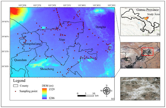
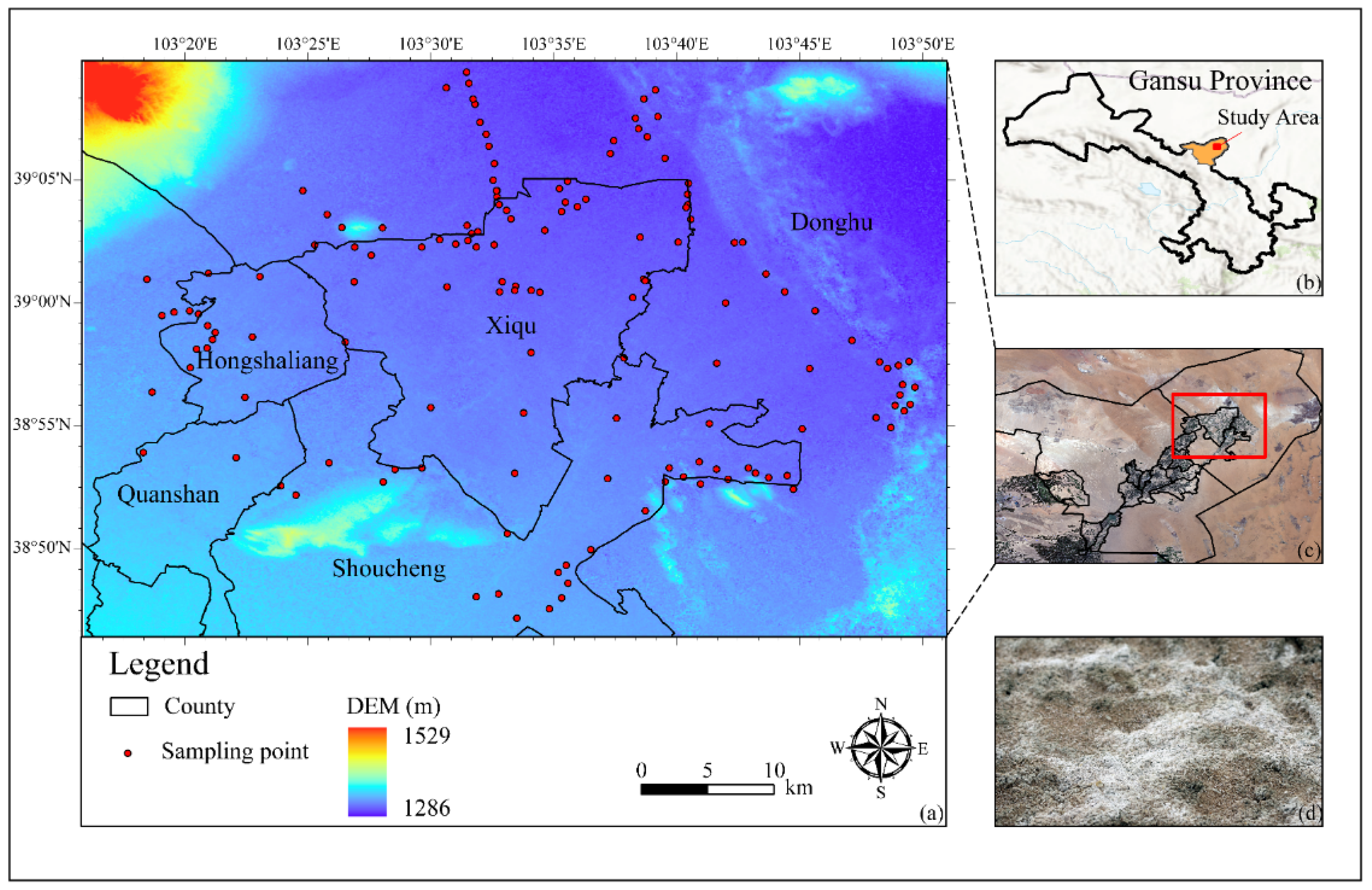
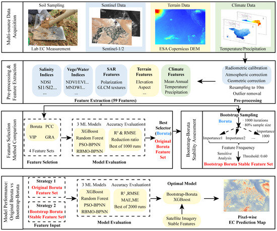
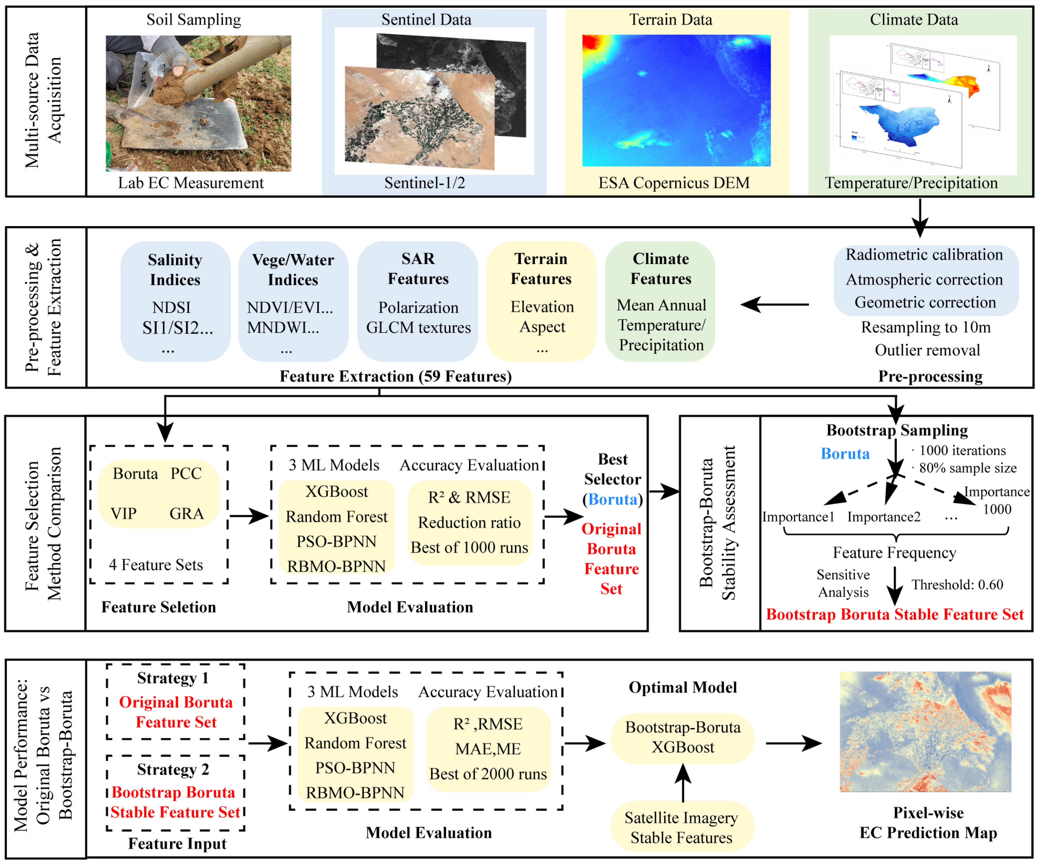
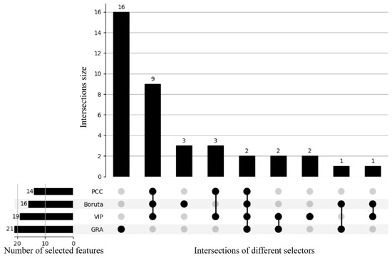
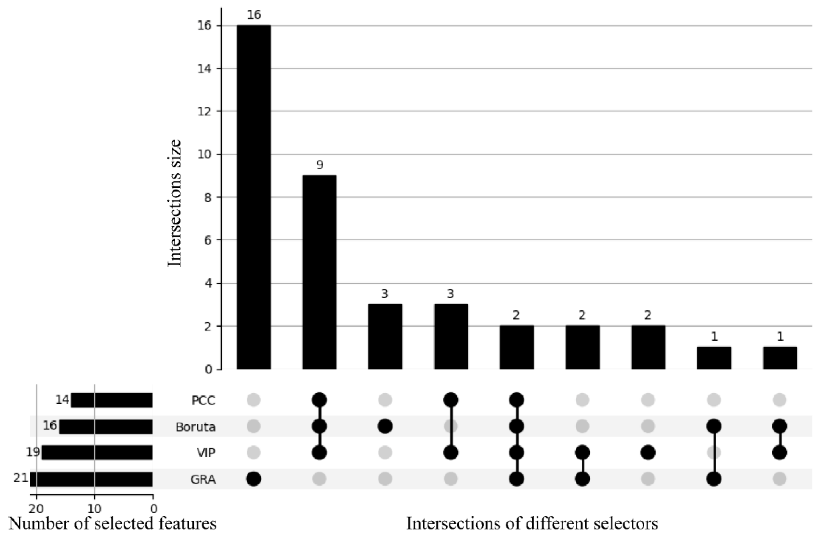
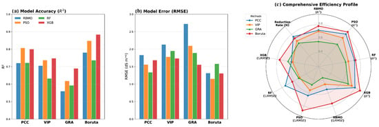
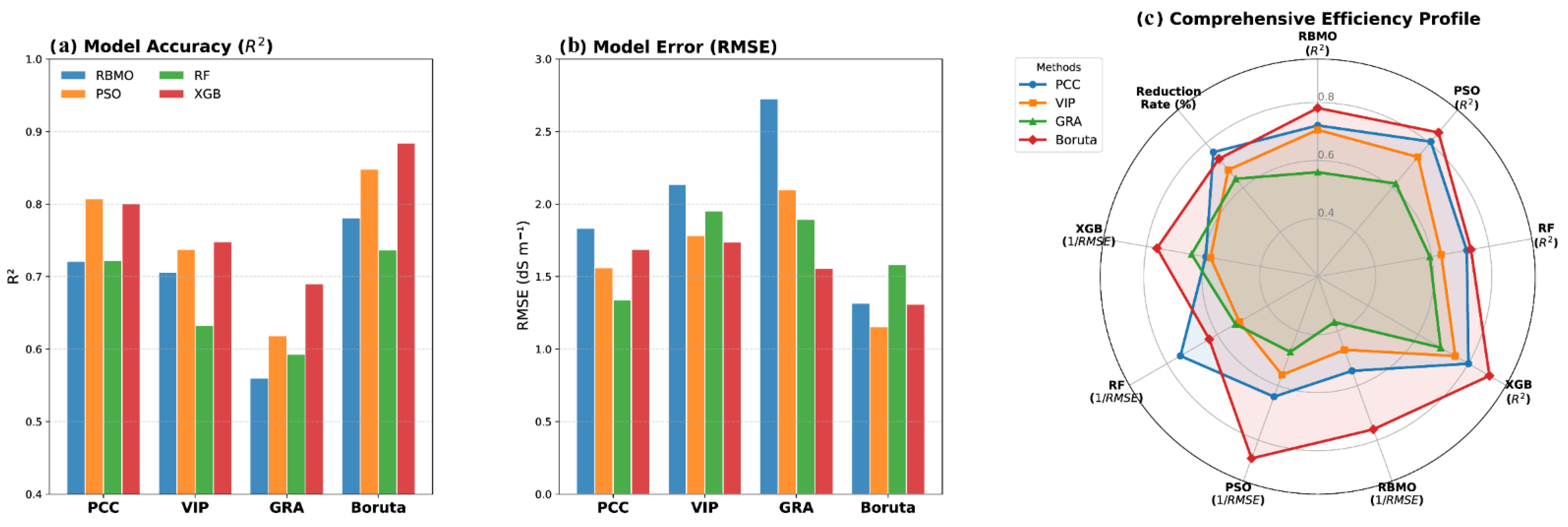
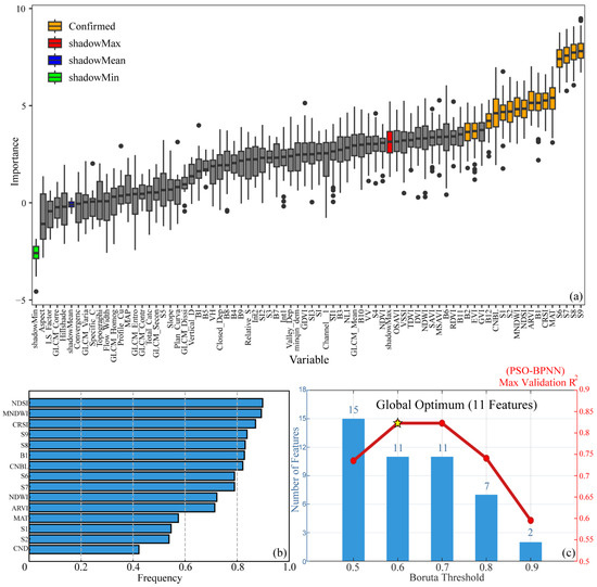
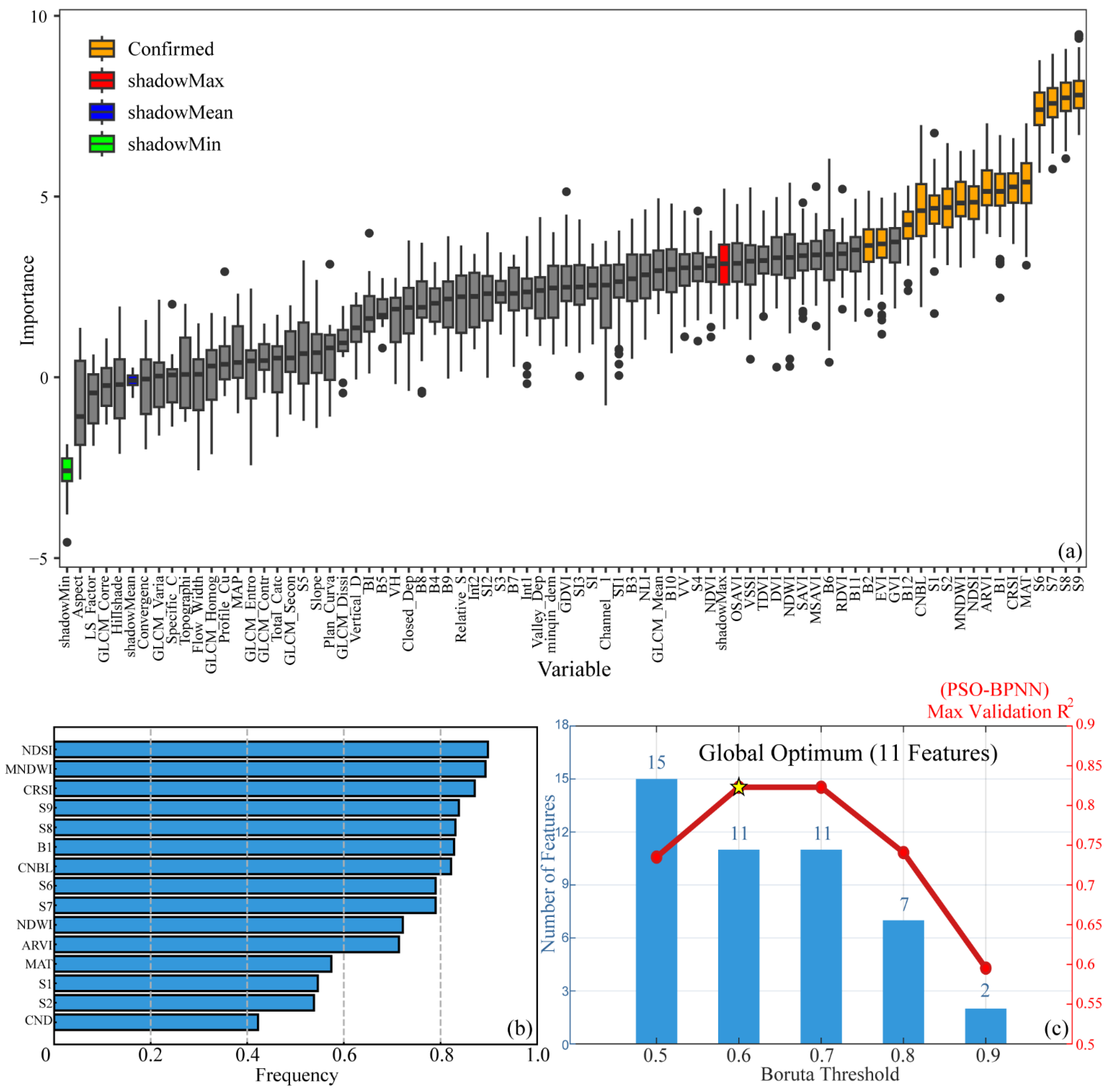
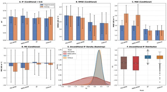
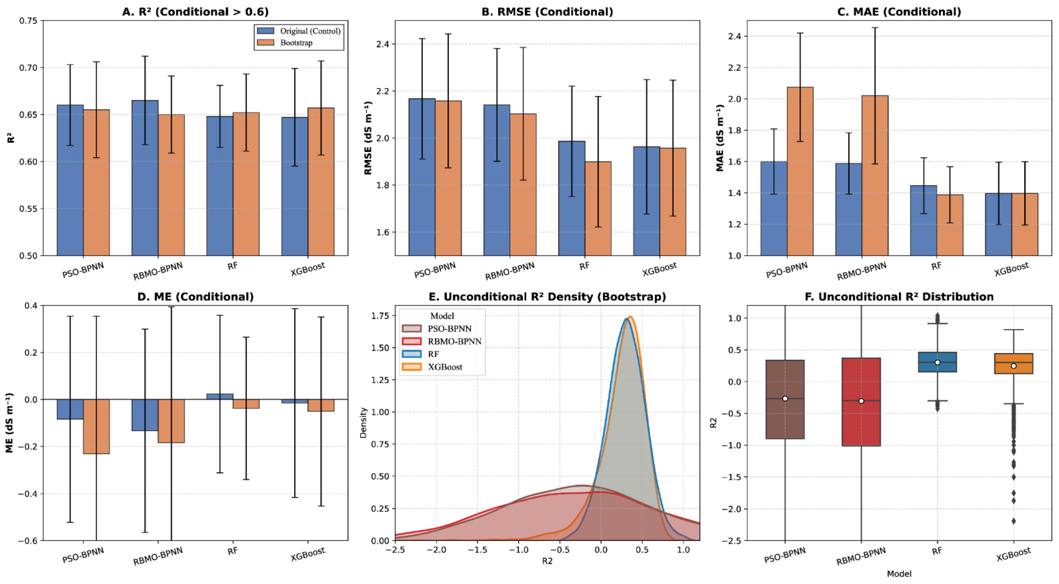
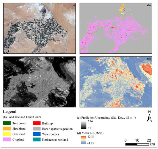
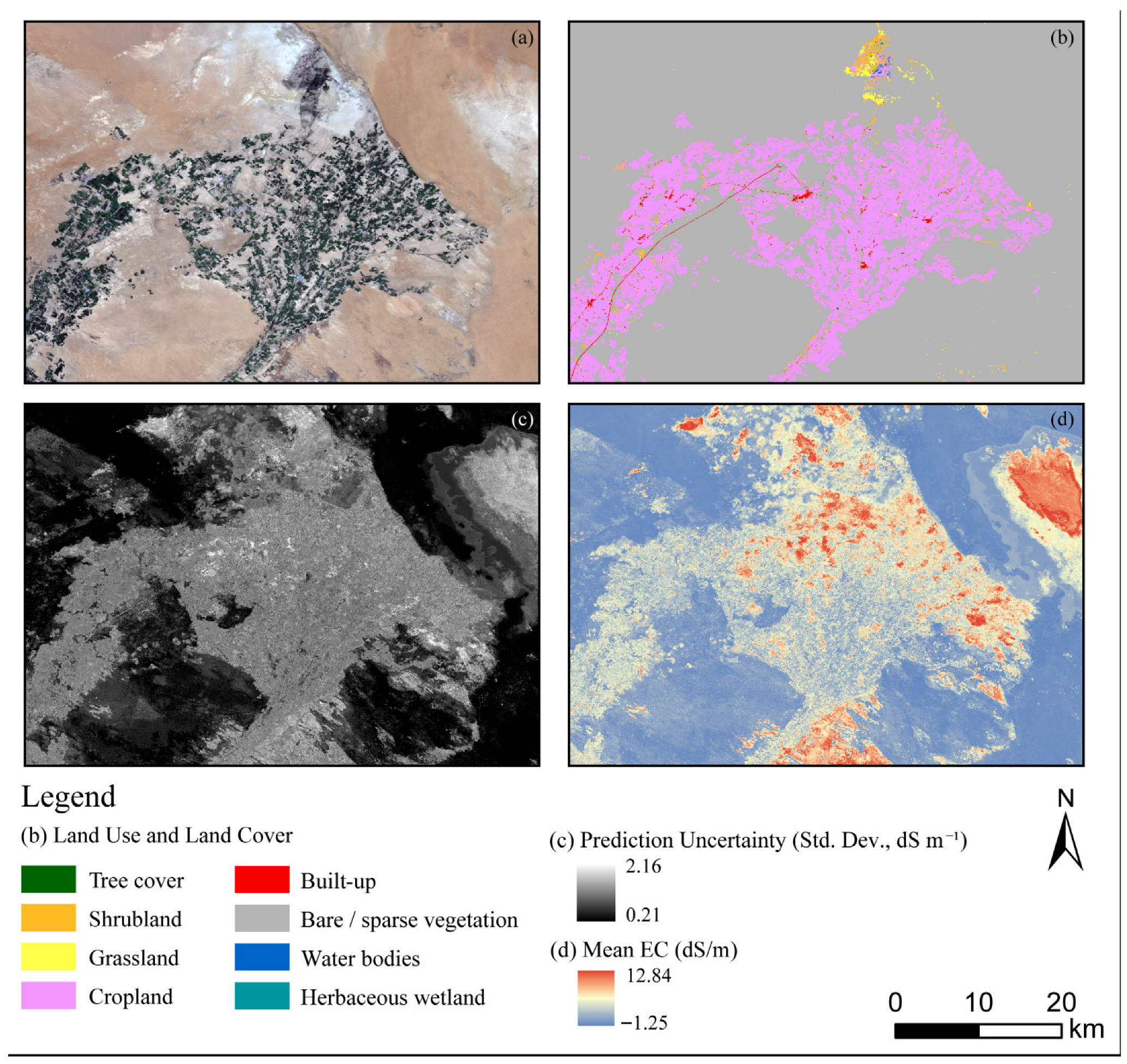
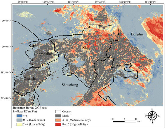
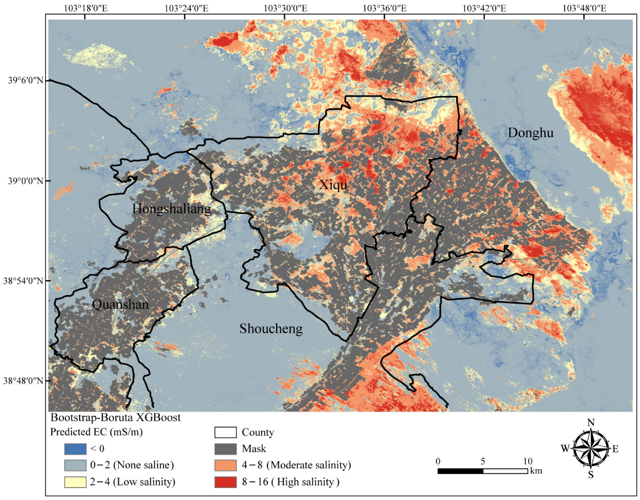

Disclaimer/Publisher’s Note: The statements, opinions and data contained in all publications are solely those of the individual author(s) and contributor(s) and not of MDPI and/or the editor(s). MDPI and/or the editor(s) disclaim responsibility for any injury to people or property resulting from any ideas, methods, instructions or products referred to in the content. |
© 2026 by the authors. Licensee MDPI, Basel, Switzerland. This article is an open access article distributed under the terms and conditions of the Creative Commons Attribution (CC BY) license.