LHRSI: A Lightweight Spaceborne Imaging Spectrometer with Wide Swath and High Resolution for Ocean Color Remote Sensing

Highlights

What are the main finding?

• This study presents a lightweight imaging spectrometer designed for water-color remote sensing and reports its preliminary on-orbit validation, which demonstrates excellent performance in both swath width and spatial resolution.

What are the implications of the main finding?

• The imaging spectrometer proposed in this study not only features a compact form factor and low manufacturing cost, but is also well suited for large-scale production and constellation deployment. In the future, it is expected to enable high-frequency observations for water-color remote sensing.

Abstract

Global water environment monitoring urgently requires remote sensing data with high temporal resolution and wide spatial coverage. However, current space-borne ocean color spectrometers still face a significant trade-off among spatial resolution, swath width, and system compactness, which limits the large-scale deployment of satellite constellations. To address this challenge, this study developed a lightweight high-resolution spectral imager (LHRSI) with a total mass of less than 25 kg and power consumption below 80 W. The visible (VIS) camera adopts an interleaved dual-field-of-view and detectors splicing fusion design, while the shortwave infrared (SWIR) camera employs a transmission-type focal plane with staggered detector arrays. Through the field-of-view (FOV) optical design, the instrument achieves swath widths of 207.33 km for the VIS bands and 187.8 km for the SWIR bands at an orbital altitude of 500 km, while maintaining spatial resolutions of 12 m and 24 m, respectively. On-orbit imaging results demonstrate that the spectrometer achieves excellent performance in both spatial resolution and swath width. In addition, preliminary analysis using index-based indicators illustrates LHRSI’s potential for observing chlorophyll-related features in water bodies. This research not only provides a high-performance, miniaturized spectrometer solution but also lays an engineering foundation for developing low-cost, high-revisit global ocean and water environment monitoring constellations.

1. Introduction

Coastal zones and inland waters, as critical ecological and economic regions, are facing multiple environmental pressures arising from climate change and anthropogenic activities, creating an urgent demand for efficient and precise remote sensing monitoring approaches [1,2,3,4]. Although traditional ground-based and airborne observation methods offer advantages in data accuracy, they exhibit significant limitations in spatial coverage, temporal responsiveness, and long-term operational costs. Benefiting from its wide-area and continuous observation capability, satellite remote sensing has become an indispensable technical pathway for aquatic environmental monitoring [5,6].

As an essential component of spaceborne optical observation, ocean color remote sensing quantitatively evaluates water quality by retrieving spectral characteristics of color-producing agents. Various satellite-borne imaging spectrometers have been developed and deployed worldwide (

Table 1. Comparison of Key Parameters of Global Ocean Color Satellites.

Satellites	ENVISAT	Aqua	Sentinel-3	HY-1E		Sentinel-2	Lantan-1
Instrument	MERIS	MODIS	OLCI	PMRIS	CZI2	MSI	LHRSI
Launch year	2002	2002	2016/2018	2023		2015/2017/2024	2025
Number of bands (380~3000 nm)	15	9	21	19	8	13	10
Swath (km)	1150	2330	1270	950	60	290	200
Spatial resolution (m)	300/1200	250/500/1000	300	100	20	10/20/60	12/24
Max weight (kg)	200 kg	229 kg	Not announced	Not announced	Not announced	290 kg	25 kg

). NASA’s Moderate Resolution Imaging Spectroradiometer (MODIS) sensor, equipped with 19 visible-to-shortwave infrared bands and a 2330 km swath, provides long-term global coverage but with a relatively coarse spatial resolution of 250–1000 m and a system mass of 229 kg [7]. The European Space Agency’s Medium Resolution Imaging Spectrometer (MERIS) and Ocean and Land Colour Instrument (OLCI), utilizing multi-camera field-of-view mosaicking, achieve swaths of 1150 km and 1270 km, respectively, and are designed specifically for global ocean color and environmental monitoring; however, their spatial resolution remains limited to 300 m [8,9,10]. China’s HY-1E satellite carries sensors such as Chinese Ocean Colour and Temperature Scanner (COCTS) and Programmable Medium Resolution Imaging Spectrometer (PMRIS), which feature extremely wide swaths (up to 3000 km) and rich spectral configurations (up to 90 channels) [11,12], but their spatial resolution remains insufficient for fine-scale monitoring of coastal and inland waters.

To better capture spatial details in nearshore and inland aquatic observations, several instruments have achieved substantial improvements in spatial resolution. For example, the second-generation Coastal Zone Imager (CZI-2) onboard HY-1E offers 20 m resolution, albeit with a limited 60 km swath, constraining regional simultaneity [13]. The Multi-Spectral Instrument (MSI) onboard the Sentinel-2 mission series achieves a favorable balance between swath width (290 km) and spatial resolution (10 m/20 m/60 m), and has become an important data source for contemporary aquatic environment monitoring. However, the mass of a single satellite reaches 290 kg [14,15,16], and the high manufacturing and launch costs significantly hinder the rapid deployment of satellite constellations and the further improvement of observation revisit frequency.

Fundamentally, achieving global water dynamics monitoring with both high spatial and temporal resolution depends on satellite constellations rather than single satellites. The extremely high cost, large size, and heavy mass of traditional Earth observation satellites severely limit the number of payloads that can be launched simultaneously, making dense constellation deployment economically and technically impractical. Consequently, advancing the miniaturization of high-performance optical payloads represents a critical step toward the realization of low-cost, high-efficiency remote sensing constellations. To date, imaging spectrometers capable of achieving 10 m spatial resolution with hundred-kilometer-scale swaths on sub-100 kg platforms—while still meeting the quantitative requirements of aquatic color remote sensing—remain scarcely reported.

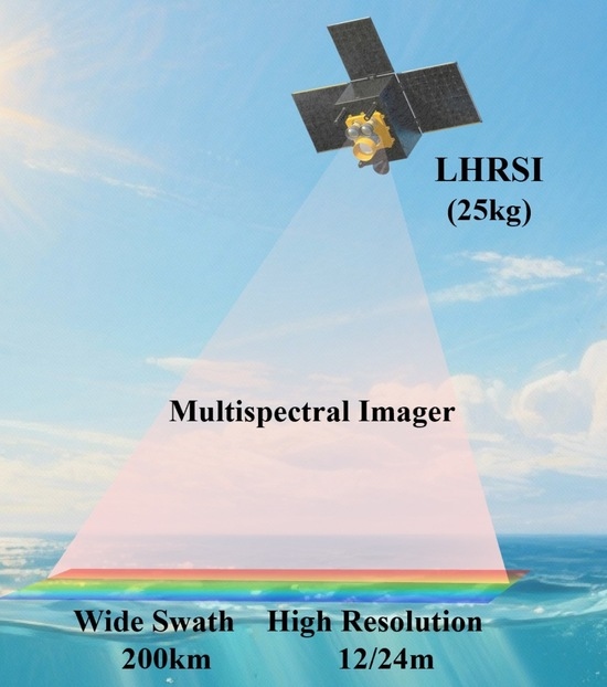
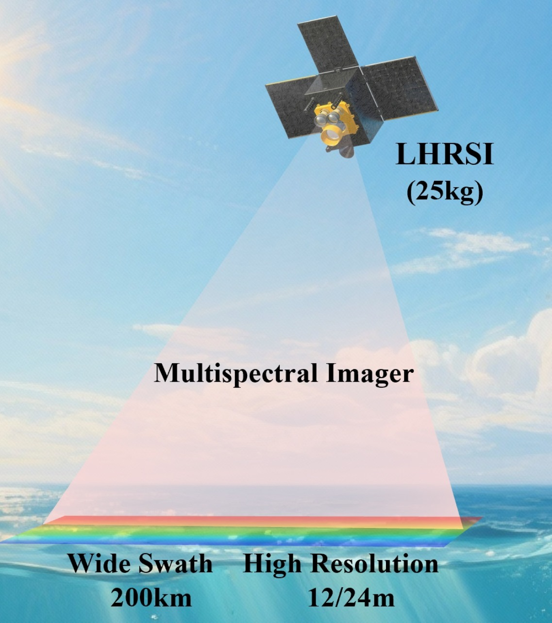
In response to these challenges, this study develops a compact, lightweight, wide-swath, high-resolution imaging spectrometer tailored for satellite-based aquatic color observation. The instrument integrates ten spectral channels spanning the visible to shortwave infrared range with a task-oriented spectral configuration that results in a relatively limited spectral coverage, but optimized for typical ocean color and inland water remote sensing applications. The visible subsystem employs a dual-camera interleaved field-of-view configuration with detector mosaicking, while the infrared subsystem utilizes a transmissive focal-plane design with staggered detector alignment. Through an innovative FOV architecture, the system achieves a hundred-kilometer-class swath and 10 m spatial resolution, while maintaining a total mass below 25 kg and power consumption below 80 W, reducing payload mass and volume by an order of magnitude. These improvements bring two major advantages: first, they significantly reduce unit cost, enabling batch production; second, they allow compatibility with micro- and nanosatellite platforms, facilitating low-cost shared launch opportunities.

On 17 January 2025, the LHRSI was successfully launched aboard the commercial satellite Lantan-1 from the Jiuquan Satellite Launch Center in China and inserted into its designated orbit. During on-orbit operations, the instrument acquired a substantial volume of high-resolution, wide-swath spectral imagery, from which preliminary chlorophyll-a concentration retrievals were performed. These results validate its potential as a core payload for future low-cost, high-revisit global water monitoring constellations.

2. Materials and Methods

This section provides a detailed description of the core technical strategies adopted in the LHRSI. Conventional high-performance imaging spectrometers typically weigh several hundred kilograms, as their performance depends on large-aperture optical systems and extensive focal plane detectors [8,14]. However, such configurations fundamentally conflict with the low-cost and rapid-deployment requirements of micro- and nanosatellite platforms. To resolve this contradiction, this study proposes a lightweight wide-swath imaging approach based on FOV fusion and detector splicing. In addition, to compensate for reduced light throughput caused by platform resource limitations, we optimize the signal-to-noise ratio (SNR) using time-delay integration (TDI).

2.1. Lightweight Wide-Swath Imaging Based on Interlaced FOV Fusion and Detector Splicing

Traditional approaches for achieving swath widths exceeding 200 km typically rely on either a single ultra-large area array detector or multiple independent optical systems for FOV stitching. The former leads to high cost and lengthy development cycles, while the latter significantly increases system volume and mass. To overcome these challenges, we introduce an FOV–detector fusion splicing method. The key idea is to maximize the utilization of the detector FOV through coordinated optical and focal plane design, while maintaining the aperture and image quality of a single optical system. This method is implemented using commercially available, moderately sized detectors, as summarized in

Table 2. Specifications of the Visible CMOS and Infrared InGaAs Detectors.

Parameter	VIS Detector	SWIR Detector
Sensor	1/1.2″CMOS	InGaAs
Wavelength	400–800 nm	950–1700 nm
Pixel size	6 µm	12.5 µm
Active pixels	4480 × 2496	1032 × 1
Quantization	10 bits	14 bits
Dimension	30.77 mm (full resolution diagonal)	12.8 mm
Weight	30.6 g	9 g

. As a result, it avoids reliance on ultra-large focal plane devices and achieves a balanced solution in terms of system performance, cost, and development efficiency.

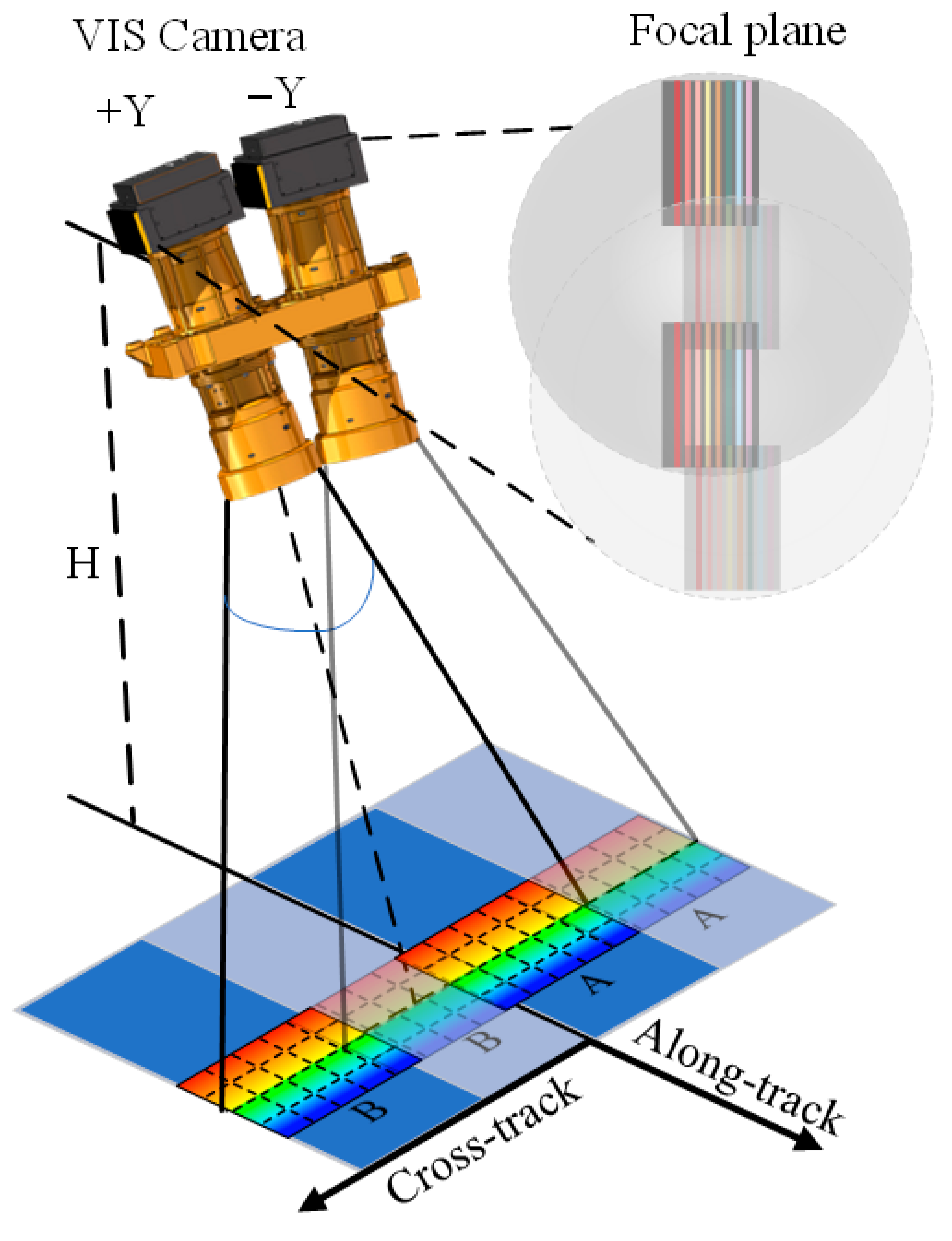
For the VIS camera, two independent transmissive optical systems are designed, with two CMOS detectors(Teledyne e2v, Inc. Milpitas, CA, USA) mounted side by side on each focal plane. Due to detector packaging and readout circuitry, a physical gap appears in the central FOV along the cross-track direction for each individual system. Rather than extending the focal plane through detector interleaving—which would increase optical system volume—we introduce a tilted dual-camera configuration. The two optical systems are installed with a slight angular offset, allowing their FOVs to overlap in the cross-track direction. In this arrangement, the missing central FOV region of the +Y camera is compensated by Detector B of the −Y camera, and vice versa. Through this “cross-compensation” fusion method, seamless FOV coverage equivalent to that of four detectors is achieved using only two optical systems (as shown in Figure 1). This design effectively expands the visible-light system’s total FOV to 23.77°, while avoiding additional optical complexity—serving as a key enabler for simultaneously achieving low mass (<25 kg) and wide swath (>200 km).

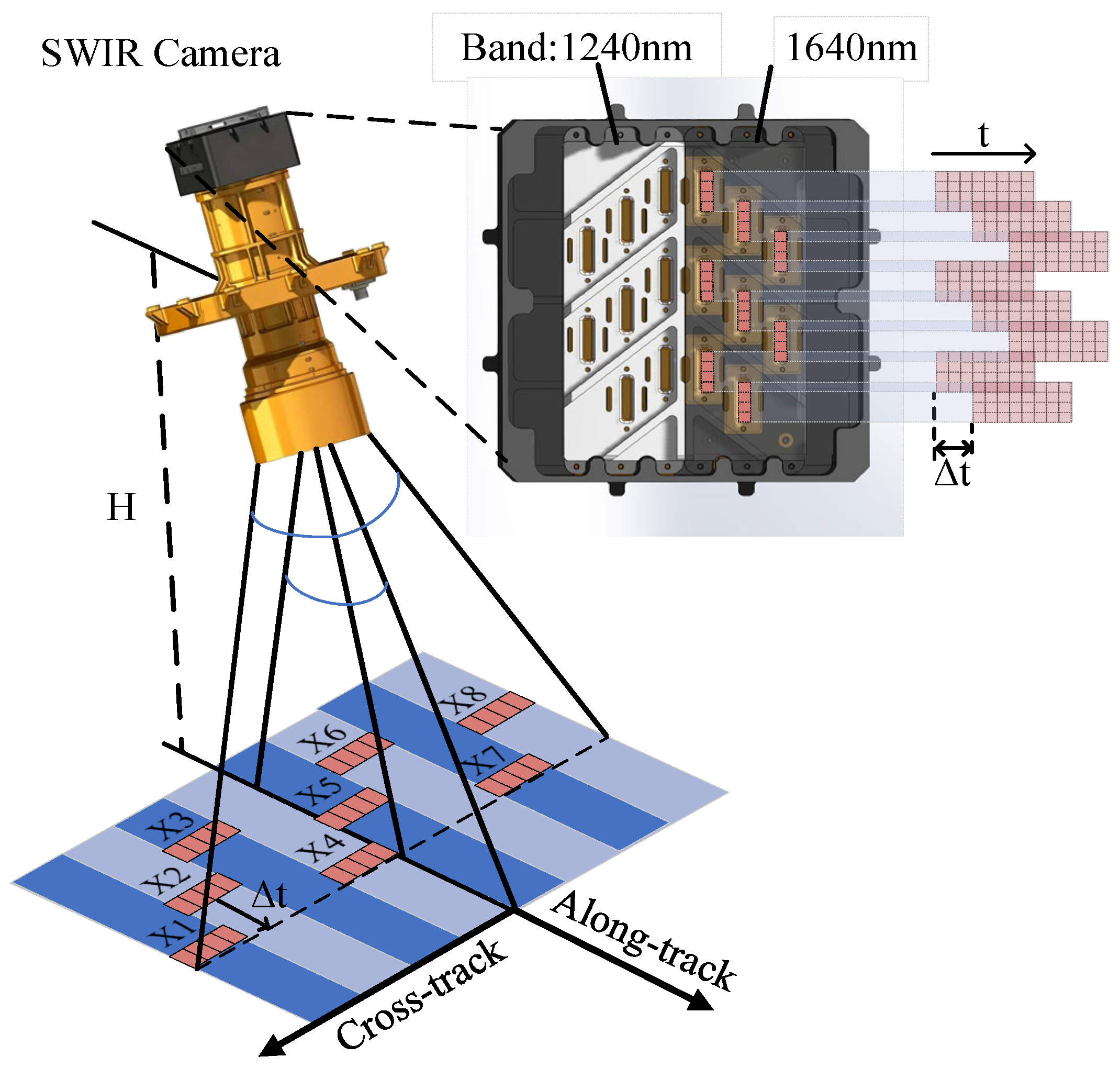
For the SWIR camera, a compact 1024 × 1 InGaAs linear detector array (Zhongke Dexin Perception Technology Co., LTD, Wuxi, China) was employed to meet the high signal-to-noise ratio requirements of atmospheric correction while maintaining a reduced system volume (see Figure 2). A multi-row staggered configuration was adopted to form a continuous field of view. The detectors were arranged in six rows on a circular focal plane to fully utilize the focal surface of the transmissive optical lens. The array is divided into two groups, with every three rows forming the focal plane for one spectral band. Adjacent detector groups share an overlap of 200 pixels. During push-broom imaging, the detectors in each group do not observe the same ground target simultaneously. Taking the 1640 nm band as an example, detectors X1, X4, and X7 capture a given ground location first. After a temporal delay of Δt, the corresponding detectors X2, X5, and X8 image the same latitude region, followed by detectors X3 and X6 after an additional delay of Δt (i.e., 2Δt in total). Consequently, the imaging of a single ground target is distributed across multiple detector rows in time rather than being acquired instantaneously. Although these temporal offsets introduce slight along-track displacements among the image strips produced by different detector rows, each detector still generates a spatially continuous push-broom imaging track. By performing a subsequent along-track alignment and strip stitching procedure, the pixel-level geometric offsets can be compensated, enabling the reconstruction of a seamless and continuous SWIR image.

This imaging strategy effectively leverages the staggered detector geometry to expand the FOV without increasing detector size, facilitating system miniaturization while maintaining high radiometric integrity and spatial continuity.

We have employed a unique FOV design to achieve wide-swath spectral image acquisition within stringent constraints on space and mass resources. This solution not only demonstrates strong engineering feasibility but also establishes a technical foundation for subsequent constellation deployment and mass production.

2.2. SNR Enhancement with Time-Delay Integration

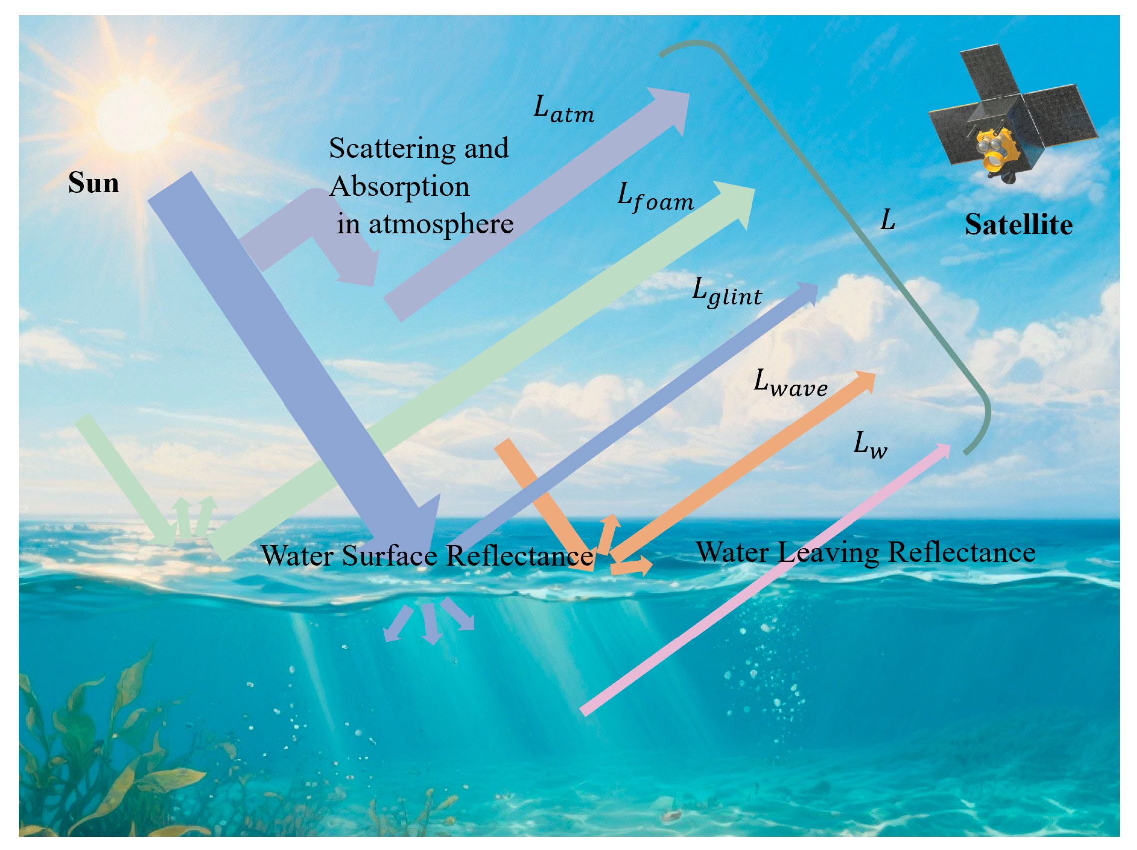
In water color remote sensing, the energy received by the sensor originates from solar radiation. This radiation is subject to atmospheric absorption and scattering before reaching the water surface. Upon incidence, solar radiation undergoes both reflection and transmission at the air-water interface. The reflection component can be categorized into specular reflection (sun glint, $L_{\mathrm{glint}}$), foam reflectance ($L_{\mathrm{foam}}$), and directional reflection from wave facets ($L_{\mathrm{wave}}$). The transmitted portion enters the water body, where it is absorbed by water molecules, phytoplankton, suspended particles, and other constituents, and undergoes multiple scattering within the water column. A fraction of this radiation is then backscattered upwards, eventually exiting the water surface as water-leaving radiance ($L_w$). Combining the above components, the total radiance ($L$) received by the satellite optical system in ocean color remote sensing can be described by the radiative transfer path (as shown in Figure 3).

The radiative transfer equation can therefore be expressed as follows:

$$L=L_{atm}+\tau {(L_{glint}+L}_{foam}+L_{wave}+L_w)$$

(1)

where τ is the atmospheric diffuse transmittance along the sensor’s viewing direction.

Remote sensing reflectance of water ($R_{rs}$) is a critical parameter for characterizing the optical properties of water bodies (ocean color constituents). However, within the total radiance detected by satellite sensors, the contribution of the water-leaving radiance is typically very small [17], imposing stringent requirements on sensor detection sensitivity.

Additionally, the need for lightweight and miniaturized payloads in space missions constrains the entrance pupil diameter of the optical system. Consequently, the number of photons collected per unit time is limited, posing a significant challenge to image SNR. To enhance SNR under low light flux conditions, the system employs TDI in the visible spectral band. When combined with push-broom imaging, this technology effectively compensates for signal loss caused by the reduced optical aperture by performing multiple exposures and accumulating signals along the flight direction for the same target.

The specific method is as follows: After superimposing the optical signals of the same target area N times, the increase in the effective signal $\overline{V_{sig}}$ is proportional to $N$, while the increase in uncorrelated noise $\overline{V_{\mathrm{noise} }}$ is proportional to the square root of N. Therefore, the signal-to-noise ratio after TDI ($SN{R}_{TDI}$) is improved by a factor of $\sqrt{N}$ compared with the original signal-to-noise ratio ($SN{R}_{\mathrm{org} }$) [18,19].

$$SN{R}_{TDI}={\displaystyle \frac{N\times \overline{V_{sig}}}{\sqrt{N}\times \overline{V_{\mathrm{noise} }}}}=\sqrt{N}{\displaystyle \frac{\overline{V_{\mathrm{sig} }}}{\overline{V_{\mathrm{noise} }}}}=\sqrt{N}SN{R}_{\mathrm{org} }$$

(2)

The instrument achieves 8-level time delay integration (TDI) in the visible light band, leading to a theoretical SNR improvement of approximately 2.8 times. This effectively offsets the inherent sensitivity disadvantage of small-aperture optical systems and ensures sufficient SNR for the detection of weak ocean color signals.

3. Spectrometer Design

3.1. Spectrometer Architecture

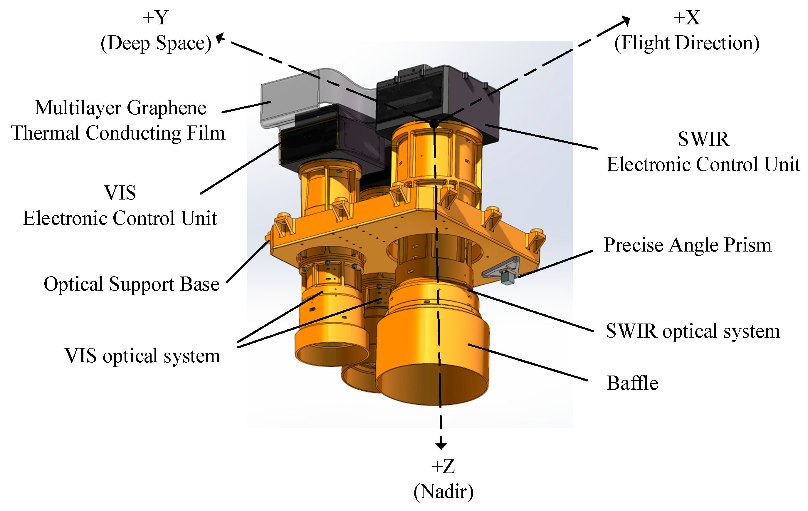
Based on the methodology described above, a VIS–SWIR imaging spectrometer has been developed. The LHRSI is characterized by a modular configuration enabling parallel development and integration of its main assemblies for schedule optimization (see Figure 4). The aluminum alloy frame incorporates mounting feet along its periphery for mechanical interface with the satellite cabin panel and simultaneously serves as the optical support structure, ensuring stable installation of the imaging subsystems. Both the VIS and SWIR cameras adopt transmissive lens configurations. The VIS and SWIR electronic control units (ECUs) are positioned behind their respective optical assemblies, and the heat generated during operation is conducted to the satellite’s +Y panel through multilayer graphene thermal conduction film (MGTCF) to ensure thermal stability.

In the structural layout, the SWIR camera is mounted vertically along the +Z direction on the optical support baseplate, while the two VIS cameras are installed on the same baseplate at their designated tilt angles to achieve the required FOV arrangement. Additionally, a precision angle prism is mounted on the +Z side of the optical support plate to provide accurate interior orientation parameters during satellite-level integration and calibration.

The LHRSI features a highly compact structural design with a total instrument mass of 24.81 kg. The visible-band subsystem consists of two VIS cameras, which employ an interleaved FOV configuration to achieve seamless coverage over a 200 km swath. The system is designed to provide 12 m spatial resolution across eight spectral bands for ocean color observation. The SWIR camera is arranged with a staggered detector configuration to match the FOV of the VIS cameras, offering 24 m spatial resolution over two spectral bands for atmospheric correction [20,21,22,23,24].

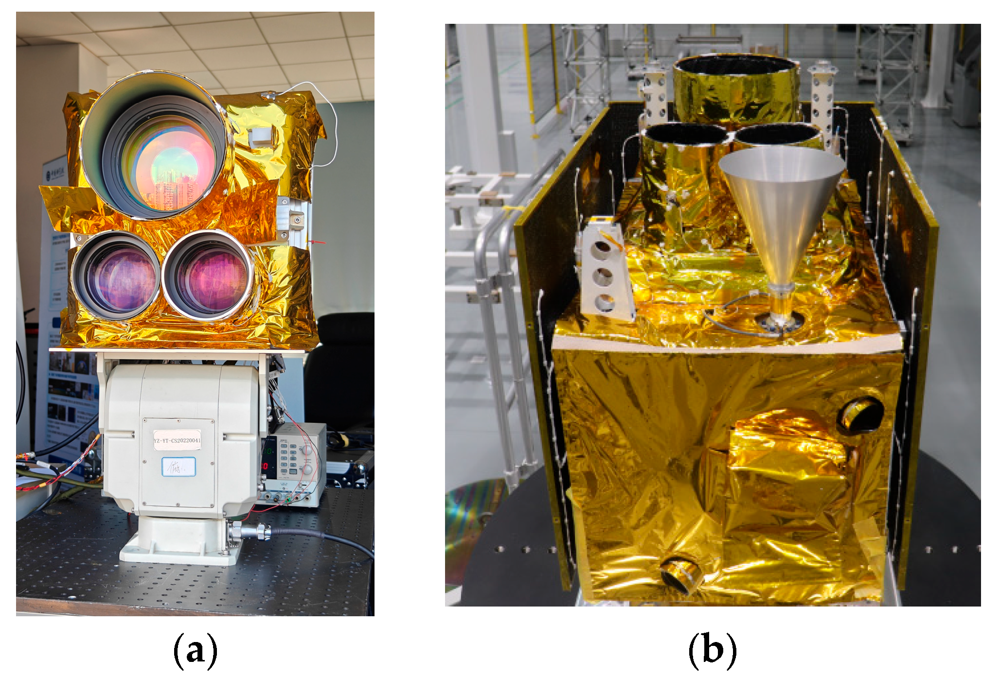
Figure 5a shows the fully assembled LHRSI mounted on a rotation stage for simulated push-broom imaging tests. Figure 5b illustrates the pre-launch integration of the instrument onboard a 70 kg-class microsatellite platform. The spectrometer was successfully launched into orbit on 17 January 2025. Detailed instrument specifications are listed in

Table 3. Detailed Specifications of the LHRSI.

Parameter	Value
Imaging mode	Push-broom Imaging
Wavelength	Visible band: Band 1: 397–427 nm Band 2: 428–458 nm Band 3: 475–505 nm Band 4: 540–570 nm Band 5: 605–635 nm Band 6: 655–685 nm Band 7: 677.5–702.5 nm Band 8: 720–760 nm SWIR band: Band 9: 1180–1300 nm Band 10: 1580–1700 nm
F-number	VIS imaging system: 3.1 SWIR imaging system: 2.6
Modulation Transfer Function	>0.1
Spatial resolution	VIS band: 12 m@500 km SWIR bands: 24 m@500 km
Swath	200 km

.

3.2. VIS Optical System Design

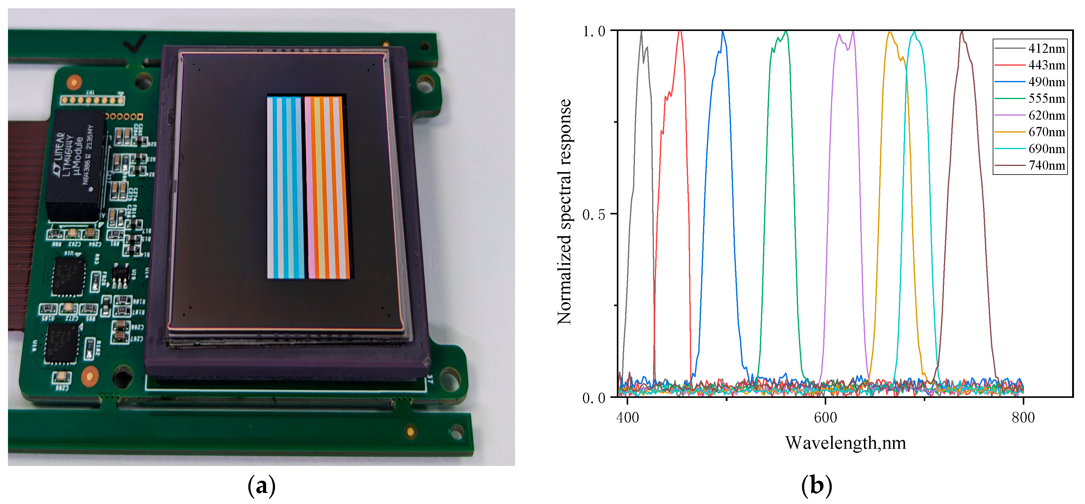
The VIS cameras are equipped with complementary metal-oxide-semiconductor (CMOS) detectors with a pixel size of 6 × 6 μm², covering the spectral range from 400 nm to 760 nm. Spectral separation is achieved using strip filters mounted directly on the CMOS detectors, enabling simultaneous acquisition of spectral and spatial information. Each filter spans 175 lines along the along-track direction, separated by a 100-line “dead space” between adjacent filters (Figure 6a). To reduce inter-channel stray light, a line-selection readout method is employed, in which only the central N lines of each channel are read. Following testing, TDI with 8-stage accumulation is implemented to enhance the SNR. The eight spectral bands are centered at 413, 443, 490, 555, 620, 670, 690, and 740 nm (Figure 6b).

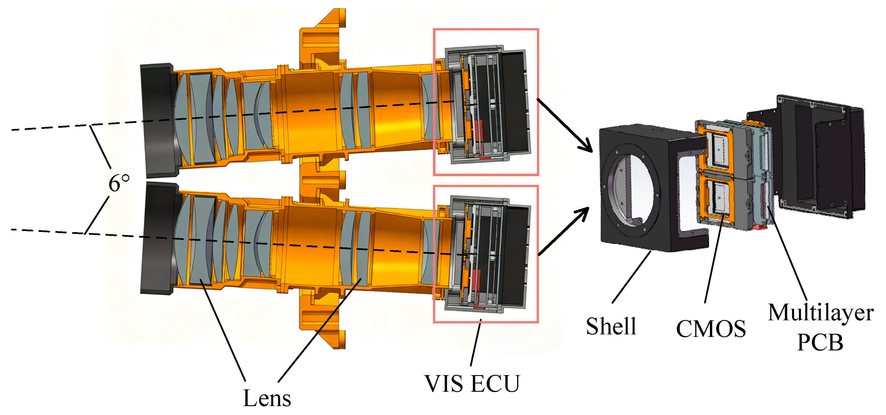
The VIS spectral camera employs a transmissive lens with an elongated tubular barrel design (see Figure 7). To facilitate assembly and alignment while maintaining manufacturability, the lens barrel is divided into two sections separated by an adjustable spacer ring. The barrel is integrally machined from 6061-T6 aluminum alloy, providing precise alignment references and benefiting from aluminum’s high thermal conductivity to minimize deformation caused by thermal gradients. The optical system consists of nine Gaussian spherical lenses, with six housed in the front barrel section and three in the rear.

Each lens provides a FOV of 17° × 2.73°, an effective aperture of 80 mm, and a focal length of 250 mm. Two modules, each equipped with a CMOS detector, are positioned along the Y-axis behind the lens. Due to packaging constraints and peripheral readout circuitry, the focal plane arrays cannot be placed contiguously, resulting in a central FOV gap for a single camera. To address this, the two visible spectral camera lenses are mounted on a baseplate with a tilt towards the +Z direction, forming a 6° angle between their optical axes. On the theoretical focal plane, the four modules corresponding to the same spectral band are arranged in an almost straight line, with a time delay of less than 100 lines between modules.

3.3. SWIR Optical System Design

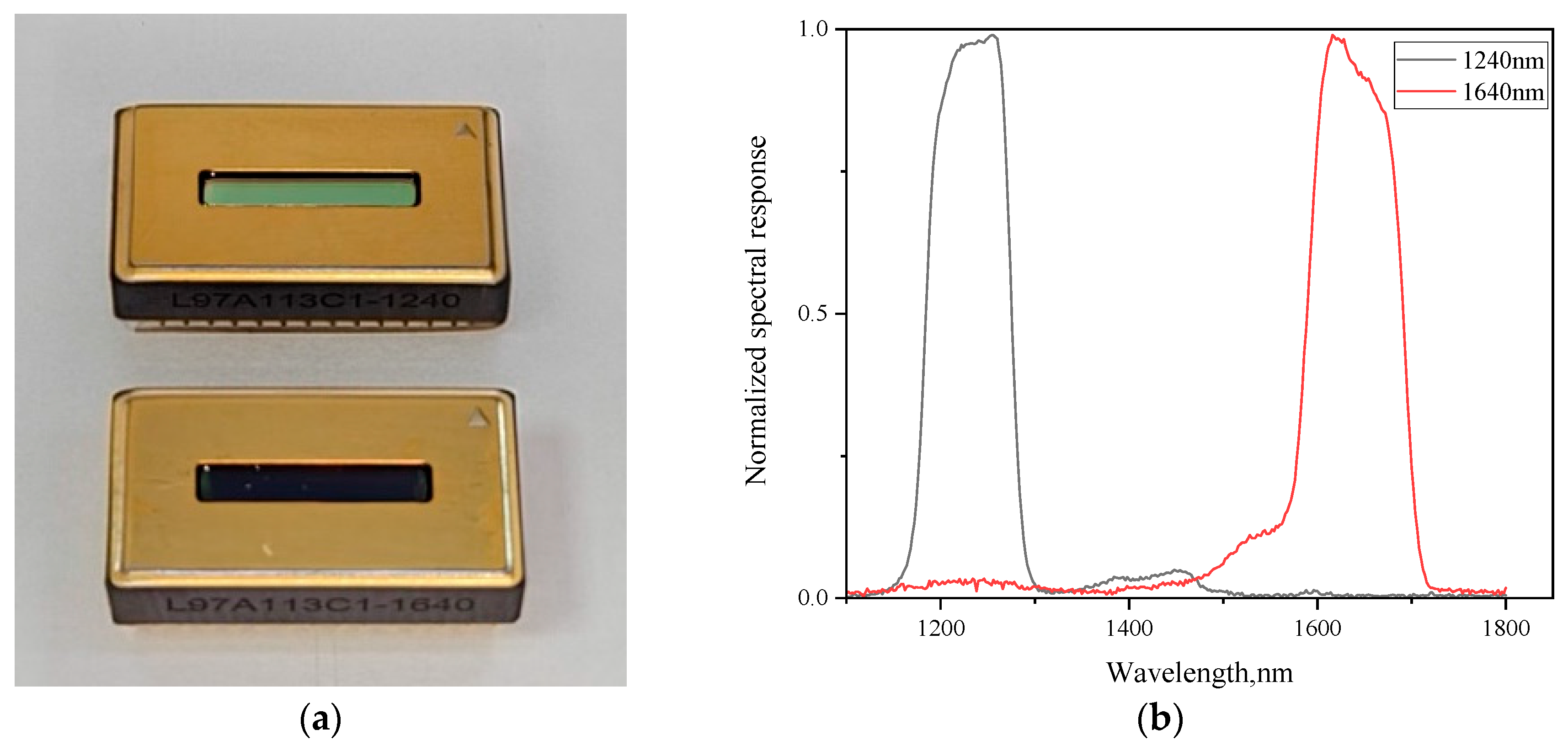
The SWIR camera is equipped with a 1024 × 1 pixel thermoelectrically cooled (TEC) InGaAs detector array, with a pixel size of 12.5 × 12.5 μm². The detector’s spectral sensitivity, determined by the InGaAs material, spans 1.4–1.7 μm (Figure 8a). To restrict the response to the target spectral bands, the detector window was replaced with a custom-designed filter during fabrication, selecting two bands centered near 1240 nm and 1640 nm (Figure 8b).

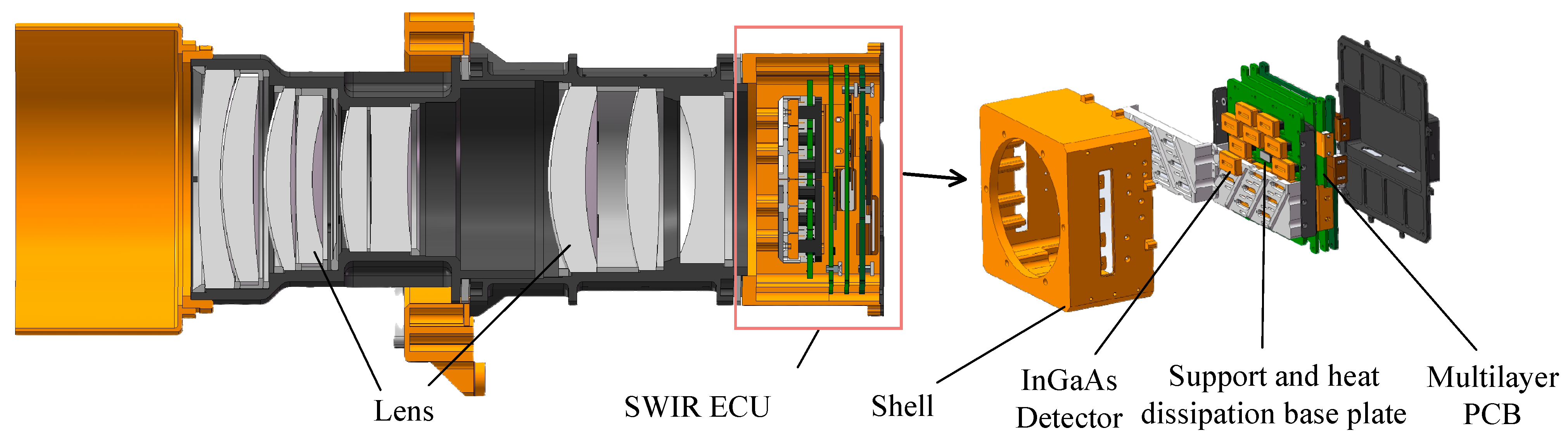
The SWIR camera employs a transmissive lens system, whose barrel design and manufacturing process are consistent with those of the visible camera(see Figure 9). Lenses are separated by aluminum alloy spacer rings, with axial spacing fine-tuned during assembly via lapping. The lens barrel is securely mounted to the main structural panel through a mid-section mounting foot. The optical system comprises eight Gaussian spherical lenses and one aspherical lens, providing a diagonal FOV of 24°, an effective aperture of 100 mm, and a focal length of 260 mm.

The SWIR detector incorporates a thermoelectric cooler (TEC) for precise temperature control, maintaining a stable operating temperature. Waste heat generated during operation is conducted to the support baseplate and subsequently dissipated to the housing through a thermal interface material, ensuring thermal stability of the optical system.

3.4. Data Flow and Temperature Control

The LHRSI employs widely adopted EIA-422 bus interfaces and Camera Link interfaces for communication with the satellite platform, enabling command transmission from the platform to the camera as well as the reception and transfer of image data. The use of these standard interfaces reduces development complexity and saves space, thereby lowering the overall cost of the camera system.

A combined active and passive thermal control strategy is implemented. Multilayer insulation is applied to external components to minimize heat loss, while a MGTCF transfers heat generated by the ECUs during operation to the satellite platform. In addition, proportion integral differential (PID) temperature control ensures precise thermal regulation of the optical unit. This strategy results in a highly mission-adapted thermal design under the stringent constraints of limited space and high integration density typical of microsatellite platforms [25].

4. Results

4.1. Ground Sampling Distance and Swath Width

Spatial resolution and FOV are critical performance metrics for an imaging spectrometer. Spatial resolution refers to the ground area represented by each detector pixel, while the FOV defines the total ground area captured in a single imaging event. High spatial resolution enables detailed observation of ground features [26,27], whereas a larger FOV improves data acquisition efficiency [28]. In satellite remote sensing, the ground sampling distance (GSD) is commonly used to quantify spatial resolution. The GSD, which depends on the detector pixel size, focal length, and orbital altitude [29,30,31], is calculated using the following equations:

$$\left\{\begin{array}{c}{IFOV}_{VIS} = {\displaystyle \frac{a_{VIS}}{f_{VIS}}} \\ {IFOV}_{SWIR} = {\displaystyle \frac{a_{SWIR}}{f_{SWIR}}}\end{array}\right.$$

(3)

$$\left\{\begin{array}{c} {GSD}_{VIS}={IFOV}_{VIS}\times H\\ {GSD}_{SWIR}={IFOV}_{SWIR}\times H\end{array}\right.$$

(4)

where ${IFOV}_{VIS}$ and ${IFOV}_{SWIR}$ denote the instantaneous FOV for the VIS and SWIR bands, respectively; $a_{\mathrm{VIS}}$ and $a_{\mathrm{SWIR}}$ are the detector pixel sizes for the VIS and SWIR bands; $f_{\mathrm{VIS}}$ and $f_{\mathrm{SWIR}}$ are the focal lengths of the optical systems for the VIS and SWIR bands; and $H$ is the orbital altitude.

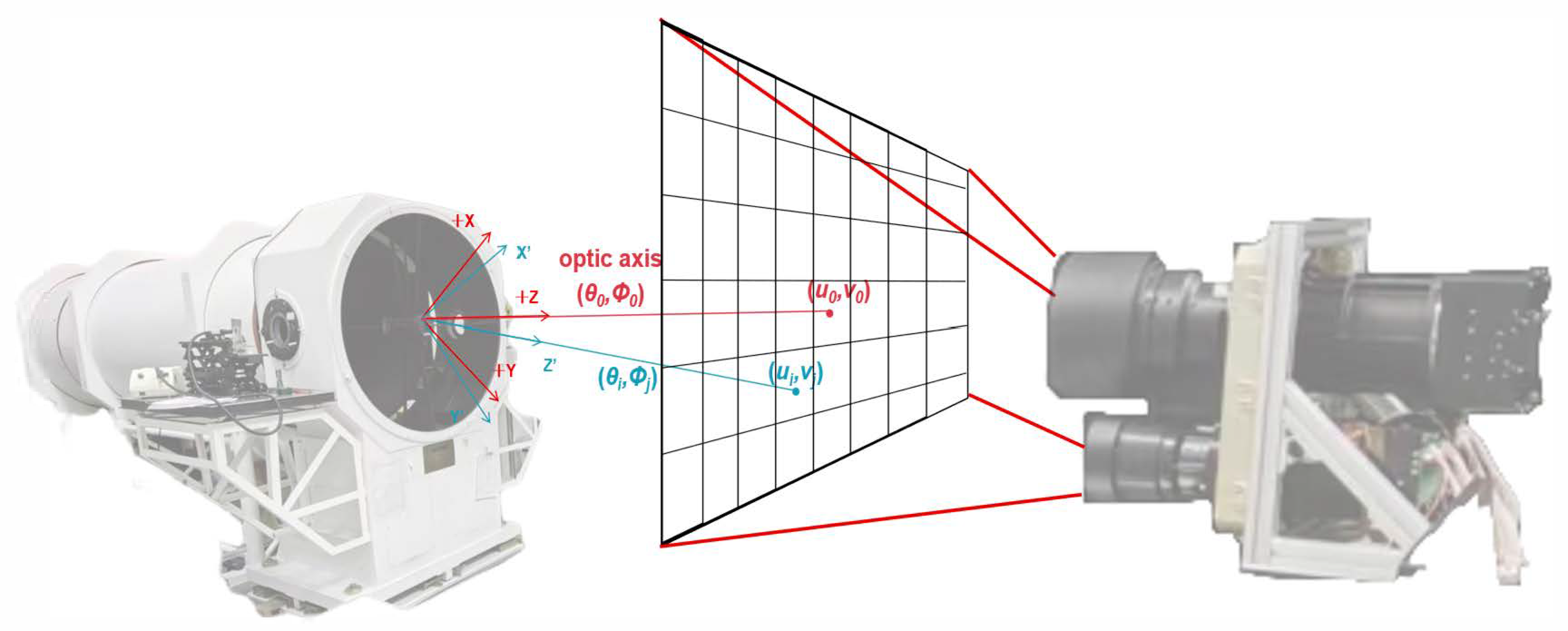
Geometric calibration establishes a precise mapping between detector pixel coordinates and incident FOV angles under controlled laboratory conditions. This is achieved using a high-precision collimator to simulate targets at infinity, allowing verification of the system’s GSD and swath width (SW). The process provides a geometric and physical basis for subsequent data mosaicking. Specifically, the imaging spectrometer is mounted on a two-dimensional rotation stage facing a large-aperture, high-collimation collimator. A point light source is placed at the collimator’s focal plane, producing a collimated beam with a known direction that enters the instrument. This parallel beam simulates a target at infinity with a defined FOV angle (see Figure 10).

Following this principle, the geometric calibration is implemented according to the following procedure:

(1)

Adjust the rotation stage until the optical axis of the instrument coincides with that of the collimator. The corresponding rotation stage readings at this position, denoted as $(A_0,{\varphi }_0)$, are defined as the zero-FOV reference. Here, ${\theta }_0$ represents the initial cross- track source incidence angle, and ${\varphi }_0$ represents the initial along- track source incidence angle. This step determines the transformation relationship between the instrument coordinate system and the rotation stage coordinate system.

(2)

The incident angle of the collimated light is varied by rotating the two-dimensional stage to position the imaging spot at predefined target coordinates $(u_i,v_j)$. The corresponding stage positions $\left({\theta }_i,{\varphi }_j\right)$ are recorded, where and j are the cross-track and along-track components of the source incidence angle espectively.

Consequently, multiple mapping pairs between the incident angles and the target coordinates are obtained. ${\mathrm{X}}_{\mathrm{i},\mathrm{j}}\left(u_i,v_j,{\theta }_i,{\varphi }_j\right)$:

$$\left(u_i,v_j\right)\rightleftharpoons \left({\theta }_i,{\varphi }_j\right)$$

(5)

In the formula, the incident angles are calculated from the stage readings $\left({\theta }_i,{\varphi }_i\right)$ and the zero reference $\left({\theta }_0,{\varphi }_0\right)$. By performing dense sampling across the entire FOV, a discrete yet accurate lookup table of pixel–incidence angle pairs covering the full target surface is obtained.

(3)

Multiple mapping pairs ${\mathrm{X}}_{\mathrm{i},\mathrm{j}}\left(u_i,v_j,{\theta }_i,\varphi \right)$, with the along-track FOV angle is fixed at $\varphi$, are selected from the lookup table. The cross-track instantaneous field of view (XTIFOV) is then calculated using the following formula:

$$XTIFOV=({\theta }_{i+1}-{\theta }_i)/\sqrt{{(u_{i+1}-u_i)}^2+{(v_{j+1}-v_j)}^2}$$

(6)

Similarly, multiple mapping pairs ${\mathrm{X}}_{\mathrm{i},\mathrm{j}}\left(u_i,v_j,{\theta }_i,\varphi \right)$, with the cross-track FOV angle is fixed at $\theta$, are selected from the lookup table. The along-track instantaneous field of view (ATIFOV) is then calculated using the following formula:

$$ATIFOV=({\varphi }_{j+1}-{\mathsf{\varphi }}_j)/\sqrt{{(u_{i+1}-u_i)}^2+{(v_{j+1}-v_j)}^2}$$

(7)

It should be noted that, due to the SWIR detector having only one pixel in the along-track direction (i.e., a single-line array), the ATIFOV for the SWIR band cannot be measured. The geometric calibration results for the VIS and SWIR bands are presented in

Table 4. The geometric calibration results of the VIS spectrometer.

Detector	IFOV		GSD
	Across-Orbit (μrad)	Along-Orbit (μrad)	Across-Orbit (m@500 km)	Along-Orbit (m@500 km)
Camera+Y_A	23.62	23.72	11.81	11.86
Camera+Y_B	23.48	23.72	11.74	11.86
Camera-Y_A	23.50	23.61	11.75	11.81
Camera-Y_B	23.53	23.64	11.77	11.82

and

Table 5. The geometric calibration results of the SWIR spectrometer.

Detector	XTIFOV ($\mathsf{\mu }\mathbf{r}\mathbf{a}\mathbf{d}$)	GSD (m@500 km)	Detector	IFOV ($\mathsf{\mu }\mathbf{r}\mathbf{a}\mathbf{d}$)	GSD ($\mathbf{m}@500\mathbf{k}\mathbf{m}$)
X1-1240	46.6962	23.3481	X1-1640	46.8606	23.4303
X2-1240	46.7197	23.3598	X2-1640	45.9446	22.9723
X3-1240	46.3204	23.1602	X3-1640	45.6191	22.8096
X4-1240	48.8337	24.4169	X4-1640	48.9511	24.4756
X5-1240	48.0116	24.0058	X5-1640	48.6223	24.3112
X6-1240	45.8271	22.9136	X6-1640	46.2768	23.1384
X7-1240	46.3708	23.1854	X7-1640	46.8606	23.4303
X8-1240	46.6527	23.3263	X8-1640	45.1259	22.5629

, respectively.

According to Equations (4), (5) and (7), the spatial resolutions of the VIS cameras in the cross-track and along-track directions are 11.78 ± 0.03 m and 11.84 ± 0.04 m, respectively. The spatial resolution of the SWIR camera is 23.11 ± 1.36 m.

With respect to the consistency and uniformity of the instantaneous IFOV across pixels, the VIS cameras exhibits excellent performance. In comparison, the SWIR cameras shows slightly lower performance, with a non-uniformity error within 6%. This error mainly arises from the intrinsic distortion of its transmissive optical lens assembly. Nevertheless, the error remains within the system tolerance and can be effectively compensated through on-orbit geometric correction algorithms.

According to the experimental results, the number of cross-track pixels in the VIS subsystem is $N_{\mathrm{VIS}}=\mathrm{17,720}$, corresponding to a total field of view of ${\mathrm{FOV}}_{\mathrm{VIS}}=23.77°$. For the SWIR camera, the cross-track pixel count is $N_{\mathrm{SWIR}}=8056$, with a total field of view of ${\mathrm{FOV}}_{\mathrm{SWIR}}=21.54°$. The system’s SW can be calculated based on the total system FOV using the following formula: The ground coverage swath of the LHRSI is expressed as:

$$\left\{\begin{array}{c}{SW}_{VIS} ={FOV}_{VIS}\times H\\ {SW}_{SWIR} ={FOV}_{SWIR}\times H\end{array}\right.$$

(8)

Based on the system design parameters, the ground swath width of the VIS subsystem is calculated to be $S{W}_{\mathrm{VIS}}=207.33 \mathrm{k}\mathrm{m}$, whereas the SWIR camera provides a swath width of $S{W}_{\mathrm{SWIR}}=187.8 \mathrm{k}\mathrm{m}$. The corresponding on-orbit experimental results are presented in detail in Section 4.2.

4.2. Signal-to-Noise Ratio

The SNR, defined as the ratio of the output signal to the detector noise, is a key metric for evaluating imaging system performance. An integrating sphere with a 25 cm output aperture was used as a stable and uniform radiance source for SNR characterization. Prior to the measurement, a Fourier Transform Spectrometer (FTS) was employed to calibrate the spectral radiance of the integrating sphere at multiple brightness levels.

During the test, the radiance level of the integrating sphere was varied to obtain time-series images under different incident irradiance conditions. The SNR for each pixel was then computed based on the temporal image sequences, followed by spectral-band averaging to derive the representative SNR of the system across varying illumination levels.

$$\left\{\begin{array}{c}{W}_{signal}^x=\overline{{DN}_x}={\displaystyle \frac{{\sum }_{n=1}^N{DN}_{x,n}}{N}}\\ W_{noise}^x=\sqrt{{\displaystyle \frac{{\sum }_{n=1}^N{\left({DN}_{x,n}-\overline{{DN}_x}\right)}^2}{N}}}\\ SNR={\displaystyle \frac{{\sum }_{x=1}^X{W}_{signal}^x/W_{noise}^x}{X}}\end{array}\right.$$

(9)

where X is the number of pixels, $N$ is the number of imaging frames, the signal intensity for each pixel $W_{signal}^x$ is the average digital number (DN) value $\overline{{DN}_x}$ of the acquired images, and the noise intensity for each pixel $W_{noise}^x$ is defined as the root mean square (RMS) deviation of the corresponding DN values [32,33].

The measured and calculated SNR for spectral bands B1 to B10 under typical radiance conditions are summarized in

Table 6. The spectral SNR results of the LHRSI.

Band Number	Central Wavelength ($\mathbf{n}\mathbf{m}$)	Band Width ($\mathbf{n}\mathbf{m}$)	Lref ($\mathbf{W}/$(${\mathbf{m}}^2·\mathbf{s}\mathbf{r}·\mathsf{\mu }\mathbf{m}$))	SNR @Lref
1	412	30	110	159
2	443	30	100	164
3	470	30	90	193
4	555	30	70	190
5	620	30	50	139
6	670	30	50	155
7	690	25	45	114
8	740	40	40	101
9	1240	120	7	300
10	1640	120	4	260

.

4.3. Radiometric Calibration

To convert the Digital Number (DN) values output by the LHRSI into physically meaningful radiance values, absolute radiometric calibration must be performed. This calibration establishes a linear response relationship between the DN values and the radiance at the entrance pupil, which can be expressed as:

$$L=G\times DN+offset$$

(10)

where $L$ is the spectral radiance at the entrance pupil, with units of $\mathrm{W}/({\mathrm{m}}^2\cdot \mathrm{sr}\cdot \mathsf{\mu }\mathrm{m})$, $G$ is the absolute radiometric calibration gain coefficient, and $offset$ represents the bias term [34].

Laboratory radiometric calibration was conducted using an integrating sphere as a uniform radiance source. A Fourier Transform Spectrometer (FTS) was used to measure the reference spectral radiance $L_{\mathrm{ref}}$ at the output port of the integrating sphere at multiple brightness levels. Simultaneously, the corresponding digital number $D{N}_{\mathrm{test}}$ from the LHRSI was recorded. The calibration coefficients, i.e., the gain $G$ and offset for each band and detector module, were derived through linear regression fitting. This process results in the radiance–DN calibration curve for the imaging spectrometer.

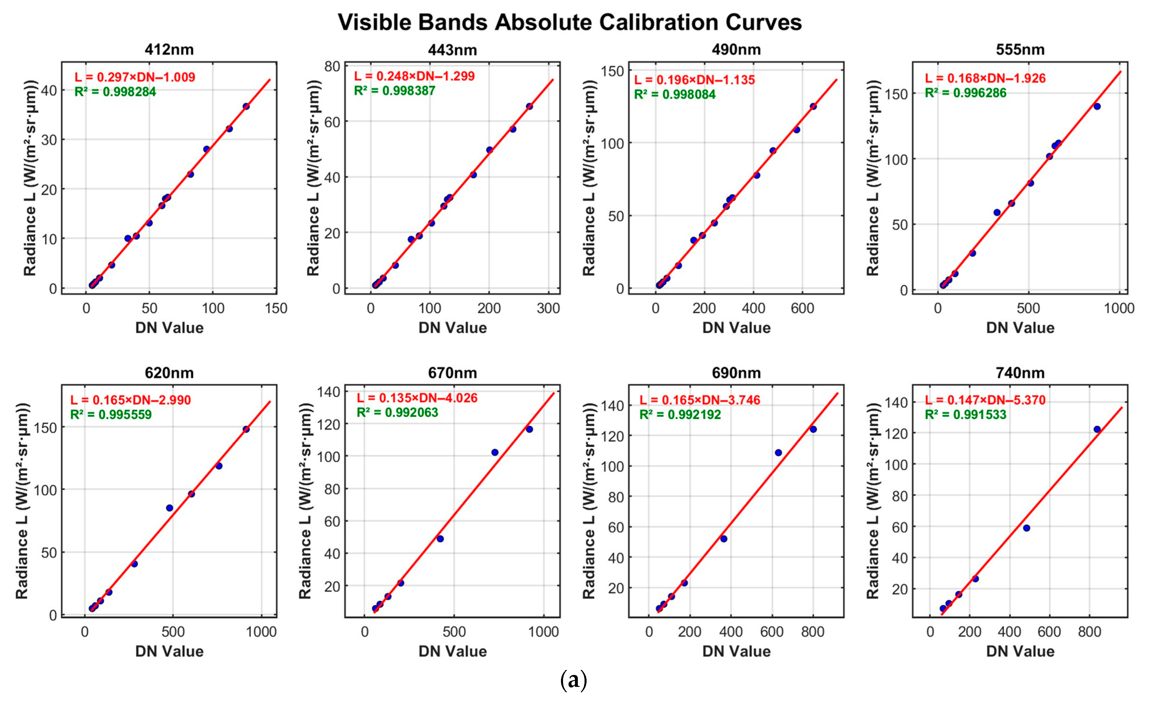
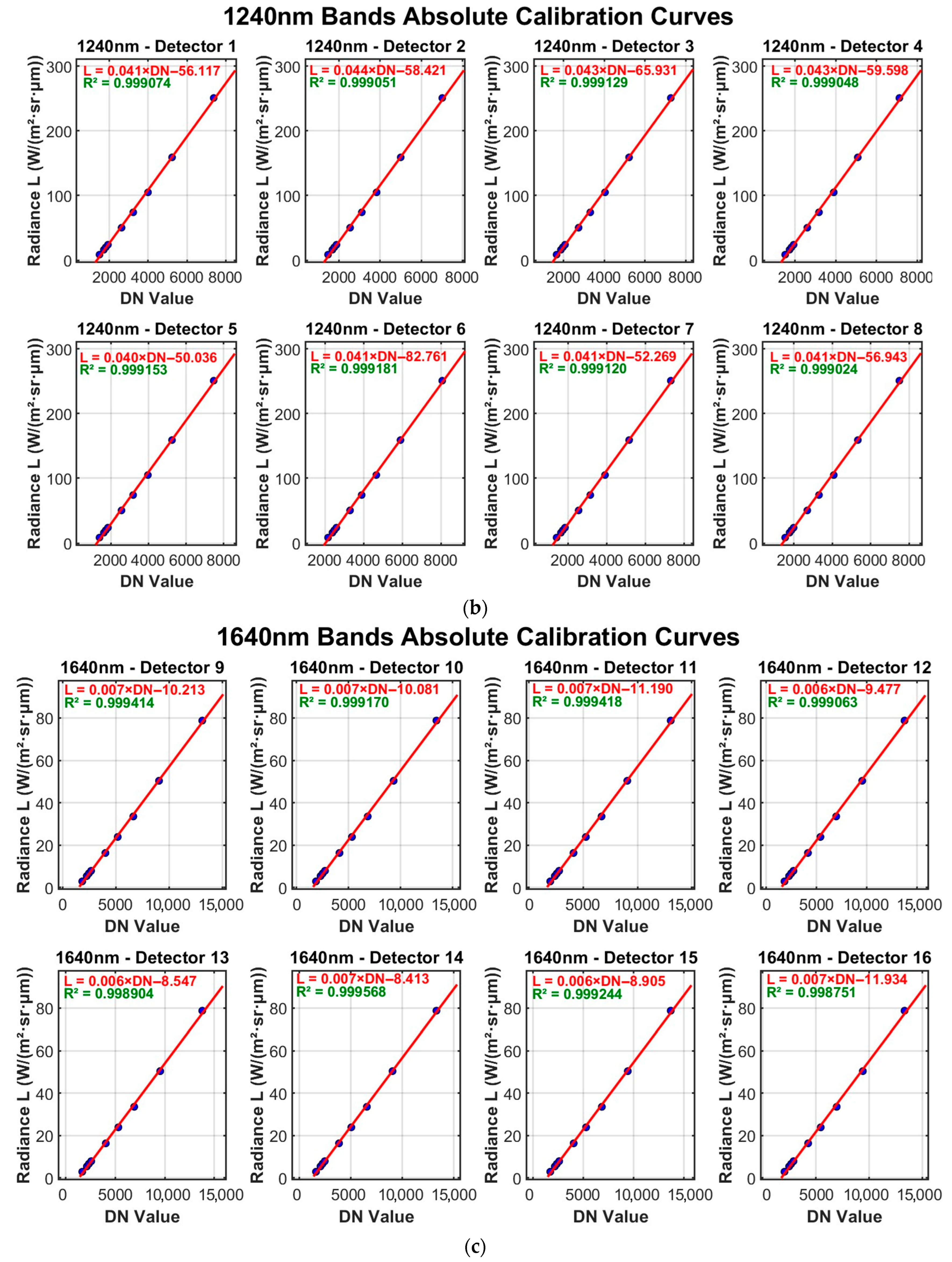
Figure 11a and Figure 11b present the radiometric calibration curves for each detector of the VIS and SWIR bands of the LHRSI, respectively. The results indicate a strong linear response between system radiance and DN values. However, distinct differences in response characteristics are observed between the VIS and SWIR bands. For the VIS bands, the intercepts of the calibration curves are close to zero, indicating negligible dark current. In contrast, the SWIR curves exhibit noticeable offsets from the origin, suggesting the presence of dark current or inherent detector noise. Additionally, the slopes of the calibration curves vary significantly across bands, reflecting differences in radiometric response sensitivity, which may be attributed to variations in filter transmittance near the respective central wavelengths. Based on these absolute calibration results, subsequent relative radiometric correction will focus on mitigating inter-band response differences and fixed-pattern noise in the SWIR band to improve image uniformity.

The calibration results indicate that the instrument exhibits excellent linear response characteristics. However, variations in response still exist among individual detector units. Therefore, relative radiometric correction is necessary to further improve image uniformity and consistency, ensuring that the data quality meets the requirements of quantitative remote sensing applications.

4.4. On-Orbit Imaging Results

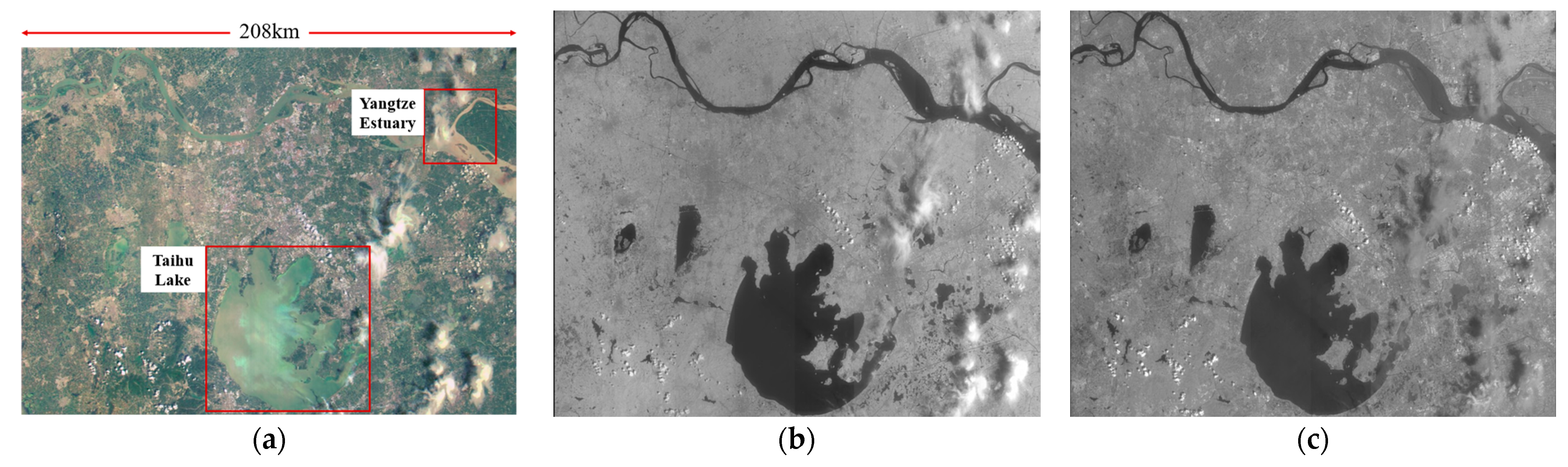
To evaluate the practical observational performance of the FOV fusion and detector splicing design, we analyzed a dataset acquired over the Lower Yangtze Plain on 29 August 2025. The scene provides nearly continuous coverage of the region (see Figure 12).

Direct extraction and measurement using the on-orbit geometric positioning data indicate actual ground swath widths of approximately 209 km for the visible bands and 187 km for the short-wave infrared bands. These findings confirm that the FOV fusion and detector splicing scheme implemented in the LHRSI effectively meets the requirement for wide-swath imaging. With this capability, the LHRSI can capture large water bodies such as Taihu Lake in a single pass. In comparison, sensors requiring multiple scene mosaics to cover the same area are more susceptible to inconsistencies caused by temporal variations in illumination and surface conditions. The wide-swath imaging capability of the LHRSI thus ensures improved spatiotemporal consistency and reliability for regional water color environment monitoring.

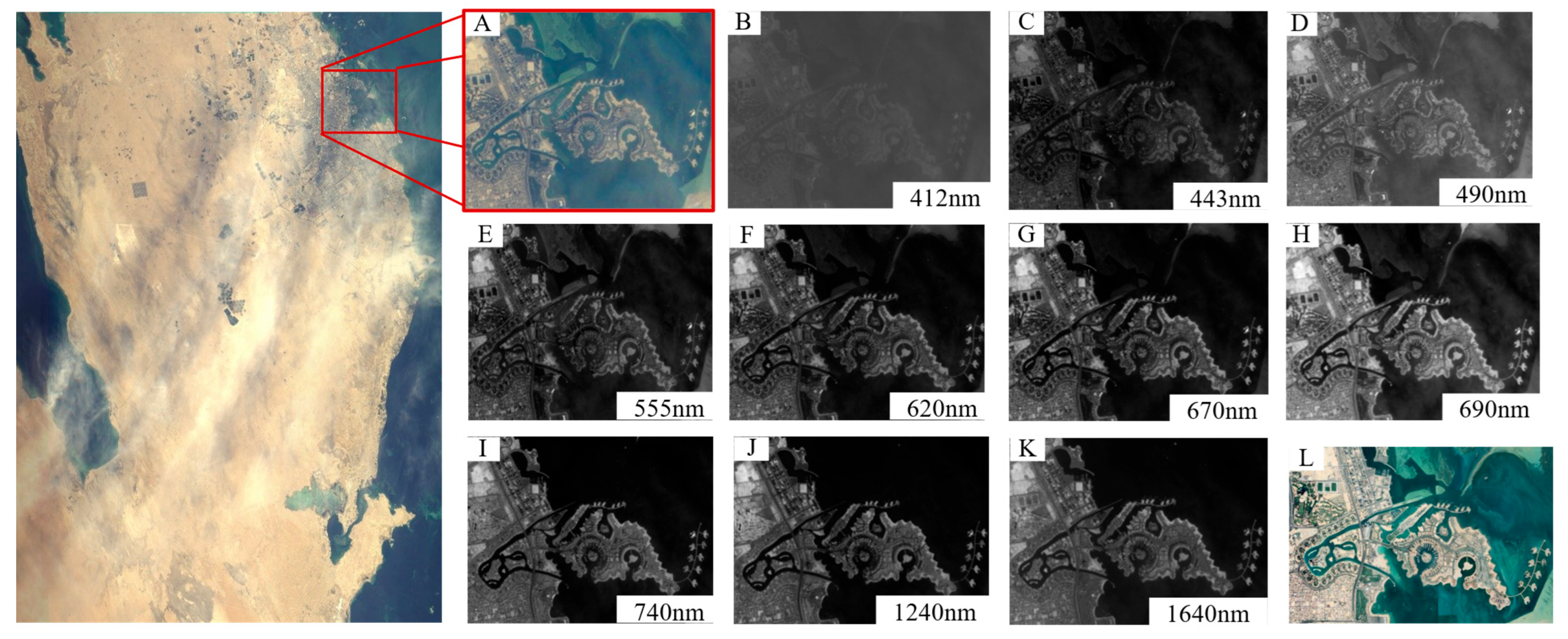
To further assess the on-orbit performance of the instrument, a spatial response analysis was conducted using the first-orbit image acquired on 18 January 2025, covering the region from the Red Sea to the Persian Gulf (see Figure 13). The slanted-edge method was applied to sharp-edged targets such as airport runways and bridges in Doha, Qatar, to derive the Modulation Transfer Function (MTF) of each spectral band at the Nyquist frequency (0.5 cycle/pixel) [35]. The results, summarized in

Table 7. MTF Measurement Results of the LHRSI at the Nyquist Frequency.

Wavelength	MTF@Nyquist (LHRSI)
412 nm	0.15
443 nm	0.17
490 nm	0.22
555 nm	0.24
620 nm	0.25
670 nm	0.27
690 nm	0.20
740 nm	0.17
1240 nm	0.35
1640 nm	0.34

, show that the LHRSI exhibits strong spectral observation capability and supports detailed characterization of surface features.

Data analysis indicates that the MTF@Nyquist values of the LHRSI in the visible bands (412–740 nm) range between 0.15 and 0.27. This performance is comparable to that of the ESA Sentinel-2 MSI sensor, whose design requirement specifies an MTF range of 0.15 to 0.3. Notably, the MTF values for the two SWIR bands (1240 nm and 1640 nm) both exceed 0.34, offering a strong spatial data foundation for their role in atmospheric correction.

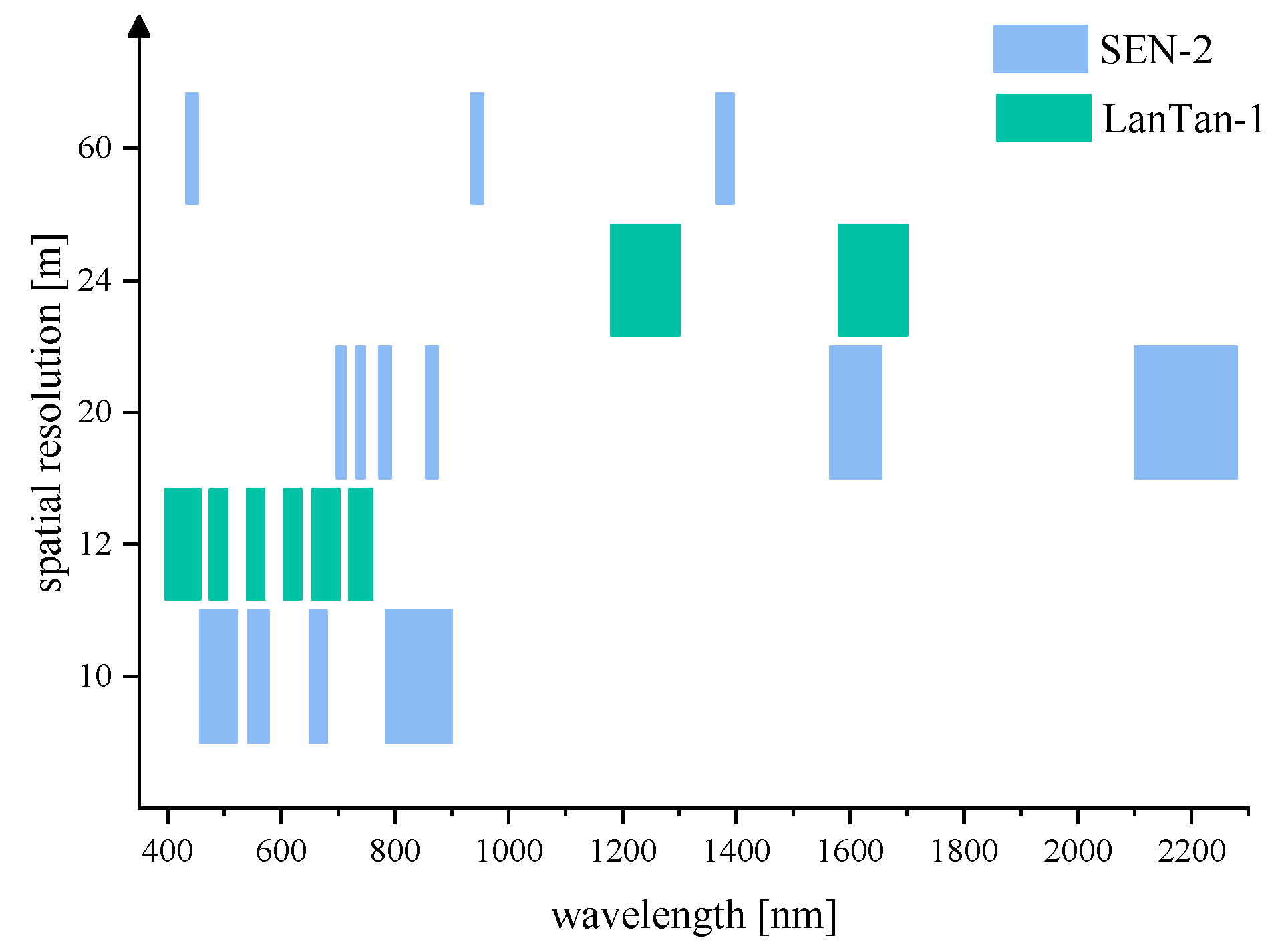
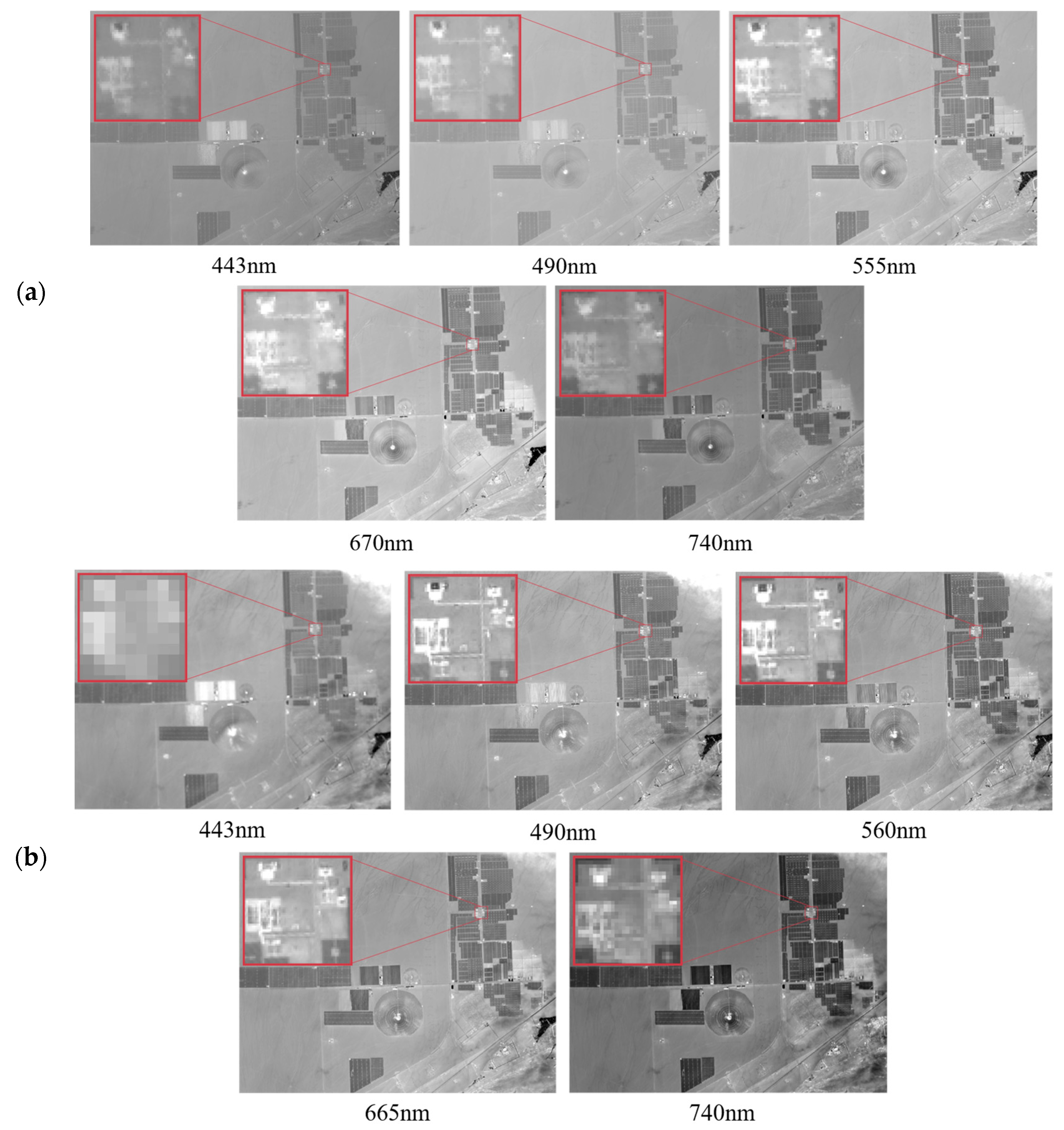
As shown in Figure 14, the band configuration of the instrument is partially comparable to that of the MSI aboard Sentinel-2A. To assess the imaging performance, observations from both sensors over the Dunhuang Calibration Site (94.48°E, 40.11°N) were compared. As illustrated in Figure 14 and Figure 15, the GSD of the LHRSI is 12 m for all visible bands and 24 m for the SWIR bands. Compared with Sentinel-2A MSI, the spatial resolution in several visible bands is improved by approximately a factor of 2 to 5, providing enhanced capability for detailed surface feature characterization, while the remaining bands deliver resolution levels comparable to MSI. Despite its lightweight and compact design, the instrument achieves a combination of wide-area coverage (on the order of 100 km swath) and 10 m-level spatial observation performance, demonstrating a balance between system miniaturization and high-quality Earth observation capability.

On-orbit test results demonstrate that the LHRSI achieves spatial resolution and image quality comparable to international mainstream operational sensors (e.g., Sentinel-2 MSI), with superior performance in several spectral bands.

4.5. Chlorophyll-Related Spectral Sensitivity over Taihu Lake

In August 2025, an extensive cyanobacterial bloom occurred in parts of the Yangtze River Basin. The LHRSI acquired multispectral data over Taihu Lake on 29 August 2025, providing an opportunity to demonstrate the instrument’s sensitivity to chlorophyll-related spectral responses in eutrophic inland waters.

As a lightweight spaceborne imaging spectrometer, the LHRSI is not equipped with an onboard radiometric calibration mechanism. At the current stage, radiometric correction of the on-orbit data relies on pre-launch laboratory calibration parameters. Continuous on-orbit radiometric calibration and performance assessment are ongoing and will be reported in future dedicated studies.

For the index-based analysis presented in this section, atmospheric effects were mitigated using the Second Simulation of a Satellite Signal in the Solar Spectrum (6S) radiative transfer model. The 6S model was employed to reduce the influence of atmospheric scattering, absorption, and illumination geometry, thereby converting top-of-atmosphere measurements into surface reflectance under consistent radiometric conditions. It should be emphasized that this processing is intended to support qualitative analysis of spectral variability rather than the generation of quantitatively validated reflectance products.

The red and red-edge spectral regions are known to be strongly influenced by chlorophyll-associated optical properties and algal photosynthetic activity. During periods of intense cyanobacterial growth, water bodies typically exhibit pronounced absorption in the red band (around 670 nm), accompanied by a rapid increase in reflectance from the red-edge to the near-infrared (NIR) region (approximately 690–740 nm) [36,37,38]. These spectral characteristics provide a physical basis for index-based indicators designed to highlight algal-related variability.

It should be noted that, due to the absence of synchronous in situ measurements and the ongoing refinement of on-orbit radiometric calibration, this study does not aim to provide quantitative chlorophyll-a concentration products. Instead, index-based indicators are employed to qualitatively illustrate the spatial variability associated with cyanobacterial bloom occurrence and to demonstrate the observation capability of the LHRSI.

In this context, the Normalized Difference Chlorophyll Index (NDCI) and the Normalized Difference Water Index (NDWI) were adopted. NDCI serves as a relative indicator sensitive to chlorophyll-related spectral features by combining the red and near-infrared bands, while NDWI was used to delineate water bodies and suppress land background interference. The two indices are defined as follows:

$$\left\{\begin{array}{c}NDCI={\displaystyle \frac{{\rho }_{NIR}-{\rho }_{RED}}{{\rho }_{NIR}+{\rho }_{RED}}}\\ NDWI={\displaystyle \frac{{\rho }_{GREEN}-{\rho }_{NIR}}{{\rho }_{GREEN}+{\rho }_{NIR}}}\end{array}\right.$$

(11)

where ${\rho }_{NIR}$, ${\rho }_{RED}$, ${\rho }_{GREEN}$ denote the water-surface reflectance in the NIR, red, and green bands, respectively. In this study, 740 nm, 670 nm, and 555 nm were selected as the representative NIR, red, and green bands for calculating the NDCI and NDWI indices. In addition, the 690 nm red-edge band was incorporated for supplementary sensitivity analysis to enhance the characterization of the algal spectral transition region. Based on these band selections, index-based spatial maps and pseudo-color composite images of Lake Taihu were generated to qualitatively demonstrate the spatial patterns related to cyanobacterial bloom distribution. 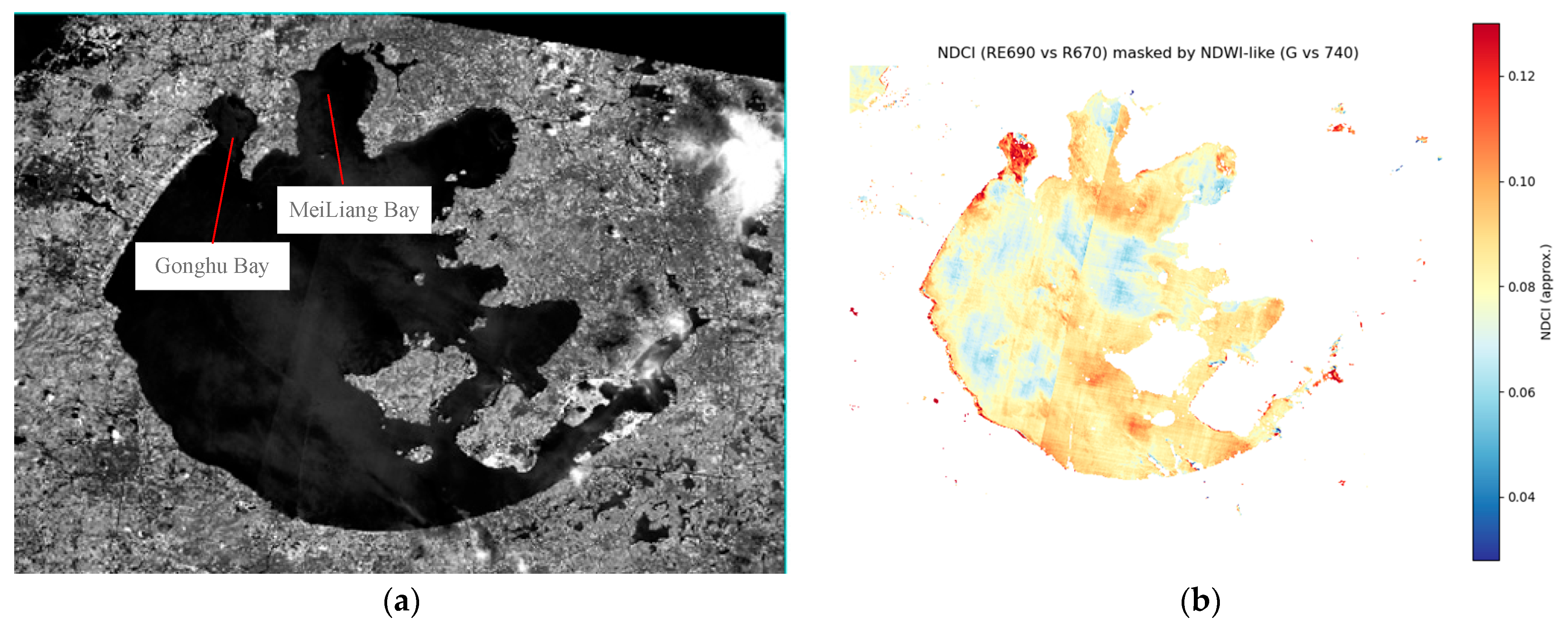Figure 16 presents the 740 nm band image and the corresponding NDCI spatial distribution, highlighting areas with elevated index values that are commonly associated with dense algal accumulation.

As shown in Figure 16, relatively higher NDCI values are observed in the northern Meiliang Bay and the northwestern Gonghu Bay regions, indicating stronger chlorophyll-related spectral responses and more pronounced bloom conditions. In contrast, the open-water areas in the central and southeastern regions showed relatively lower NDCI values, suggesting comparatively weaker algal presence. It should be noted that elevated index values may also occur in shallow-water regions or areas with high suspended sediment concentrations, which can introduce spectral interference and affect the index response.

4.6. Ulva Prolifera Monitoring

In July 2025, A large-scale Ulva prolifera bloom appeared in the Yellow Sea. On July 11, the Sentinel-2 satellite overpassed the region 282 s prior to the LHRSI. The corresponding imaging results from both platforms are shown in Figure 17a. To facilitate direct comparison, the two images were co-registered based on terrestrial features present in the scene. The co-registration outcome is presented in Figure 17b, in which the red channel represents Sentinel-2 data, and the white overlay corresponds to the measurements acquired by LHRSI.

By extracting the leading edges of multiple Ulva aggregation zones from the 740 nm band images of both sensors as feature points, the pixel displacement of their centroids was calculated over a 282 s interval. This displacement was then converted to geographic displacement using the GSD of the respective instruments, yielding the drift velocity. Based on this estimation, the Ulva prolifera generally exhibited a predominantly northward drift on that day, with a drift velocity of approximately 0.1418 m/s in the nearshore area and about 0.1021 m/s in the offshore area.

This case demonstrates that the LHRSI can be effectively integrated into a multi-satellite collaborative observation framework, providing a high-temporal-resolution monitoring solution for rapidly evolving transient phenomena, including ecological disasters, sudden environmental pollution events, and extreme weather processes.

5. Discussion

By adopting an interleaved dual-field-of-view and detector splicing fusion design for the VIS subsystem, together with a transmissive focal-plane configuration employing staggered detector arrays for the SWIR subsystem, the LHRSI achieves wide-swath spectral imaging within a total instrument mass of less than 25 kg. On-orbit experimental results further verify that the system simultaneously delivers 10 m-class spatial resolution and a swath width exceeding 200 km at an orbital altitude of 500 km. Such a performance combination on a sub-25 kg spaceborne imaging spectrometer has been scarcely reported in existing ocean color remote sensing missions, highlighting the novelty and engineering significance of the proposed design.

Compared with current mainstream ocean color and multispectral sensors, the LHRSI occupies a distinct position in terms of observation capability and mission orientation. Sensors such as MODIS, MERIS, OLCI, and PMRIS provide extremely wide swaths that are well suited for monitoring of open oceans, yet their relatively coarse spatial resolution limits their effectiveness in resolving fine-scale features in coastal and inland waters. In contrast, high-resolution instruments such as the CZI-2 offer enhanced spatial detail but suffer from narrow swath widths, which restrict regional coverage and reduce temporal revisit capability. The Sentinel-2 MSI achieves an excellent balance between spatial resolution and swath width; however, its large satellite mass and associated launch and manufacturing costs constrain dense constellation deployment. Against this backdrop, the LHRSI offers a complementary solution by combining 10 m-class spatial detail with hundred-kilometer-class coverage on a lightweight platform, making it particularly suitable for constellation-based deployment and rapid regional observation. Moreover, the Ulva prolifera monitoring case demonstrates the potential of the LHRSI to operate synergistically with existing ocean color satellites, enabling multi-sensor collaborative observations that enhance temporal resolution and monitoring robustness for rapidly evolving aquatic phenomena.

At its current stage of development, the LHRSI is particularly well suited for high-resolution, wide-swath monitoring of aquatic environments. While the on-orbit imaging results confirm the instrument’s strong observational capability, further efforts are required to fully support quantitatively validated water color products. These efforts include long-term evaluation of on-orbit radiometric calibration stability and the continued development of atmospheric correction algorithms optimized for the instrument’s specific spectral and geometric characteristics.

6. Conclusions

This study successfully demonstrates the development and on-orbit performance of the LHRSI, a lightweight, wide-swath, high-resolution imaging spectrometer designed for ocean color remote sensing. With a total mass of 24.81 kg, the instrument achieves 10 m-class spatial resolution and a swath width exceeding 200 km at an orbital altitude of 500 km. These capabilities enable the LHRSI to strike a balance between high spatial resolution and wide coverage, providing an efficient solution for future low-cost, high-revisit satellite constellations dedicated to water environment monitoring.

While the instrument has proven effective in acquiring high-resolution spectral data, further advancements are necessary to fully support quantitatively validated water color products. Future work will focus on refining the on-orbit radiometric calibration processes, improving atmospheric correction algorithms, and optimizing the system’s stability to ensure the consistent reliability of the data. These efforts will enhance the LHRSI’s capacity to support global ocean and inland water monitoring applications, contributing to the development of next-generation ocean color remote sensing technologies.

Despite these achievements, certain limitations remain. Currently, radiometric correction is based on pre-launch calibration results, and changes may have been introduced during launch and on-orbit operation. These effects need to be corrected with ground-based auxiliary measurements, and the long-term stability of the instrument’s on-orbit radiometric calibration requires evaluation through extended monitoring to ensure the consistency and reliability of data products. In addition, atmospheric correction algorithms optimized for the instrument’s specific characteristics are still under development. Future work will focus on these aspects, further enhancing the demonstrated capability and potential of this instrument for observing ocean color features, paving the way for future quantitative applications.

References

- Akram, H.; Hussain, S.; Mazumdar, P.; Chua, K.O.; Butt, T.E.; Harikrishna, J.A. Mangrove Health: A Review of Functions, Threats, and Challenges Associated with Mangrove Management Practices. Forests 2023, 14, 1698. [Google Scholar] [CrossRef] [Scilit]
- Hao, Z.; Xu, M.; Zou, X.; Wang, C. The Changing Changjiang River Estuarine-Coastal Ocean Continuum in the Anthropocene. Catena 2024, 238, 107904. [Google Scholar] [CrossRef] [Scilit]
- Alava, J.J.; Cheung, W.W.L.; Ross, P.S.; Sumaila, U.R. Climate Change–Contaminant Interactions in Marine Food Webs: Toward a Conceptual Framework. Glob. Change Biol. 2017, 23, 3984–4001. [Google Scholar] [CrossRef] [Scilit] [PubMed]
- Comer-Warner, S.; Brekenfeld, N.; Romeijn, P.; Ullah, S.; Gooddy, D.; Kettridge, N.; Marchant, B.; Hannah, D.; Mao, F.; Krause, S. Closing the Climate-Hydrology Feedback Loop: Variations in Greenhouse Gas Fluxes Resulting from Changes in Catchment Hydrology Due to Human-Induced Climate Change. In Proceedings of the EGU General Assembly Conference Abstracts, Online, 19–30 April 2021; p. EGU21-1617. [Google Scholar]
- Chen, L.; Liu, L.; Liu, S.; Shi, Z.; Shi, C. The Application of Remote Sensing Technology in Inland Water Quality Monitoring and Water Environment Science: Recent Progress and Perspectives. Remote Sens. 2025, 17, 667. [Google Scholar] [CrossRef] [Scilit]
- Chen, J.; Chen, S.; Fu, R.; Li, D.; Jiang, H.; Wang, C.; Peng, Y.; Jia, K.; Hicks, B.J. Remote Sensing Big Data for Water Environment Monitoring: Current Status, Challenges, and Future Prospects. Earth’s Future 2022, 10, e2021EF002289. [Google Scholar] [CrossRef] [Scilit]
- Barnes, W.L.; Xiong, X.; Salomonson, V.V. Status of Terra MODIS and Aqua MODIS. In Proceedings of the IGARSS 2002: IEEE International Geoscience and Remote Sensing Symposium and 24th Canadian Symposium on Remote Sensing, Toronto, ON, Canada, 24–28 June 2002; IEEE: New York, NY, USA, 2002; Volumes I–VI, pp. 970–972. [Google Scholar]
- Rast, M.; Bezy, J.L.; Bruzzi, S. The ESA Medium Resolution Imaging Spectrometer MERIS a Review of the Instrument and Its Mission. Int. J. Remote Sens. 1999, 20, 1681–1702. [Google Scholar] [CrossRef] [Scilit]
- Nieke, J.; Borde, F.; Mavrocordatos, C.; Berruti, B.; Delclaud, Y.; Riti, J.B.; Garnier, T. The Ocean & Land Colour Imager (OLCI) for the Sentinel 3 GMES Mission: Status and First Test Results. In Proceedings of the Earth Observing Missions and Sensors: Development, Implementation, and Characterization II, Kyoto, Japan, 30 October–1 November 2012; Shimoda, H., Xiong, X., Eds.; SPIE—The International Society for Optical Engineering: Washington, DC, USA, 2012; Volume 8528, p. 85280C. [Google Scholar]
- Nieke, J.; Mavrocordatos, C.; Berruti, B. Sentinel-3A: First Commissioning Results of Its Optical Payload. In Proceedings of the Sensors, Systems, and Next-Generation Satellites XX, Edinburgh, Scotland, 26–28 September 2016; SPIE—International Society for Optics and Photonics: Washington, DC, USA, 2016; Volume 10000, pp. 55–63. [Google Scholar]
- Zhang, K.; Wang, L.; Yan, C. System Design and Develop of the New-Generation Ocean Color Observation Satellite. Spacecr. Recovery Remote Sens. 2025, 46, 27–39. [Google Scholar] [CrossRef]
- Yang, T.; Xu, P.; Fu, Z.; Duan, P.; Li, S.; Hu, B.; Wang, J.; Zhang, K. Design and Implementation of New Generation Ocean Color and Temperature Scanner System. Spacecr. Recovery Remote Sens. 2025, 46, 49–62. [Google Scholar] [CrossRef]
- Zhang, X.; Chu, B.; Zheng, J.; Li, T.; Gao, Y.; Liu, X.; Li, K.; Fan, J.; Cao, W.; Wang, M. Design and Verification of the Coastal Zone Imager on the New Generation Ocean Color Satellite. Spacecr. Recovery Remote Sens. 2025, 46, 40–48. [Google Scholar] [CrossRef]
- Drusch, M.; Del Bello, U.; Carlier, S.; Colin, O.; Fernandez, V.; Gascon, F.; Hoersch, B.; Isola, C.; Laberinti, P.; Martimort, P. Sentinel-2: ESA’s Optical High-Resolution Mission for GMES Operational Services. Remote Sens. Environ. 2012, 120, 25–36. [Google Scholar] [CrossRef] [Scilit]
- Gascon, F.; Bouzinac, C.; Thépaut, O.; Jung, M.; Francesconi, B.; Louis, J.; Lonjou, V.; Lafrance, B.; Massera, S.; Gaudel-Vacaresse, A. Copernicus Sentinel-2A Calibration and Products Validation Status. Remote Sens. 2017, 9, 584. [Google Scholar] [CrossRef] [Scilit]
- Pandžic, M.; Mihajlovic, D.; Pandžic, J.; Pfeifer, N. Assessment of the Geometric Quality of Sentinel-2 Data. Int. Arch. Photogramm. Remote Sens. Spat. Inf. Sci. 2016, 41, 489–494. [Google Scholar] [CrossRef] [Scilit]
- Tan, W.; He, H.; Chen, X.; Qi, W. Analyzing the Influence of Atmosphere on Optical Remote Sensing in 400 to 2500 Nm Wavelength Spectrum. In Proceedings of the AOPC 2020: Optical Spectroscopy and Imaging; and Biomedical Optics, Beijing, China, 30 November–2 December 2020; SPIE—The International Society for Optical Engineering: Washington, DC, USA, 2020; Volume 11566, pp. 103–108. [Google Scholar]
- Lepage, G.; Bogaerts, J.; Meynants, G. Time-Delay-Integration Architectures in CMOS Image Sensors. IEEE Trans. Electron Devices 2009, 56, 2524–2533. [Google Scholar] [CrossRef] [Scilit]
- Cheng, K.-W.; Yin, C.; Hsieh, C.-C.; Chang, W.-H.; Tsai, H.-H.; Chiu, C.-F. Time-Delay Integration Readout with Adjacent Pixel Signal Transfer for CMOS Image Sensor. In Proceedings of the Technical Program of 2012 VLSI Design, Automation and Test, Hsinchu, Taiwan, 23–25 April 2012; IEEE: New York, NY, USA, 2012; pp. 1–4. [Google Scholar]
- Shanmugam, P. CAAS: An Atmospheric Correction Algorithm for the Remote Sensing of Complex Waters. Ann. Geophys. 2012, 30, 203–220. [Google Scholar] [CrossRef] [Scilit]
- Liu, H.; Zhou, Q.; Li, Q.; Hu, S.; Shi, T.; Wu, G. Determining Switching Threshold for NIR-SWIR Combined Atmospheric Correction Algorithm of Ocean Color Remote Sensing. ISPRS J. Photogramm. Remote Sens. 2019, 153, 59–73. [Google Scholar] [CrossRef] [Scilit]
- Xue, C.; Chen, S.; Lee, Z.; Hu, L.; Shi, X.; Lin, M.; Liu, J.; Ma, C.; Song, Q.; Zhang, T. Iterative Near-Infrared Atmospheric Correction Scheme for Global Coastal Waters. ISPRS J. Photogramm. Remote Sens. 2021, 179, 92–107. [Google Scholar] [CrossRef] [Scilit]
- Werdell, P.J.; Franz, B.A.; Bailey, S.W. Evaluation of Shortwave Infrared Atmospheric Correction for Ocean Color Remote Sensing of Chesapeake Bay. Remote Sens. Environ. 2010, 114, 2238–2247. [Google Scholar] [CrossRef] [Scilit]
- Wang, M. Remote Sensing of the Ocean Contributions from Ultraviolet to Near-Infrared Using the Shortwave Infrared Bands: Simulations. Appl. Opt. 2007, 46, 1535–1547. [Google Scholar] [CrossRef] [Scilit]
- Song, Y.; Lu, L.; Cheng, B.; Li, Z.; Tang, G.; Li, Q.; Liu, S.; Li, C.; Zhao, B.; Qi, H. Thermal Design and On-Orbit Performance of Remote Sensing Cameras on Commercial Microsatellites. Appl. Therm. Eng. 2025, 281, 128505. [Google Scholar] [CrossRef] [Scilit]
- Frasson, R.P.M.; Ardila, D.R.; Pease, J.; Hestir, E.; Bright, C.; Carter, N.; Dekker, A.G.; Thompson, D.R.; Green, R.O.; Held, A. The Impact of Spatial Resolution on Inland Water Quality Monitoring from Space. Environ. Res. Commun. 2024, 6, 101003. [Google Scholar] [CrossRef] [Scilit]
- Wang, F.; Chen, C.; Liu, F.; Yue, R.; Kong, X. A High-Confidence Resolution Enhancement Method for Geostationary Hyperspectral Remote Sensing Images. In Proceedings of the Tenth Symposium on Novel Optoelectronic Detection Technology and Applications, Taiyuan, China, 1–3 November 2024; SPIE—The International Society for Optical Engineering: Washington, DC, USA, 2025; Volume 13511, pp. 1316–1323. [Google Scholar]
- Grøtte, M.E.; Birkeland, R.; Honoré-Livermore, E.; Bakken, S.; Garrett, J.L.; Prentice, E.F.; Sigernes, F.; Orlandić, M.; Gravdahl, J.T.; Johansen, T.A. Ocean Color Hyperspectral Remote Sensing with High Resolution and Low Latency—The HYPSO-1 CubeSat Mission. IEEE Trans. Geosci. Remote Sens. 2021, 60, 1–19. [Google Scholar] [CrossRef] [Scilit]
- Su, Z.; Zhong, X.; Zhang, G.; Li, Y.; He, X.; Wang, Q.; Wei, Z.; He, C.; Li, D. High Sensitive Night-Time Light Imaging Camera Design and in-Orbit Test of Luojia1-01 Satellite. Sensors 2019, 19, 797. [Google Scholar] [CrossRef] [Scilit]
- Bakken, S.; Henriksen, M.B.; Birkeland, R.; Langer, D.D.; Oudijk, A.E.; Berg, S.; Pursley, Y.; Garrett, J.L.; Gran-Jansen, F.; Honoré-Livermore, E. Hypso-1 Cubesat: First Images and in-Orbit Characterization. Remote Sens. 2023, 15, 755. [Google Scholar] [CrossRef] [Scilit]
- Lin, G.G.; Semple, A.; Tan, B.; Zhang, P. A Review on Sensor Spatial Resolution and a Proposal on Grid Pixel Sizing. In Proceedings of the European Space Agency (ESA) Very High-Resolution Radar and Optical Data Assessment (VH-RODA) Workshop, Frascati, Italy, 27–30 November 2023. [Google Scholar]
- Hu, S.; Chen, S.; Ma, C.; Song, Q.; Wang, J.; Li, S.; Peng, H.; Ye, X. On-Orbit Intrinsic Characterization and Radiometric Performance of the Primary Sensor Onboard the Chinese New-Generation Ocean Color Observation Satellite. IEEE Trans. Geosci. Remote Sens. 2025, 63, 1–21. [Google Scholar] [CrossRef] [Scilit]
- Li, L.; Jiang, Y.; Shen, X.; Li, D. Long-Term Assessment and Analysis of the Radiometric Quality of Standard Data Products for Chinese Gaofen-1/2/6/7 Optical Remote Sensing Satellites. Remote Sens. Environ. 2024, 308, 114169. [Google Scholar] [CrossRef] [Scilit]
- Yang, Y.; Liu, S.; Wang, P.; Yuan, L.; Tang, G.; Liu, X.; Lu, J.; Kong, Y.; Li, C.; Wang, J. Uncooled Snapshot Infrared Spectrometer with Improved Sensitivity for Gas Imaging. IEEE Trans. Instrum. Meas. 2024, 73, 4506009. [Google Scholar] [CrossRef] [Scilit]
- Boreman, G.D. Modulation Transfer Function in Optical and Electro-Optical Systems; SPIE—The International Society for Optical Engineering: Washington, DC, USA, 2001; Volume 4. [Google Scholar]
- Zhang, L.; Ma, C.; Chen, X.; Zhang, C.; Li, Q.; Ye, X.; Tian, L. An Integrated Algorithm to Estimate Chlorophyll-a Concentration in Various Optical Waters Using HY-3A CZI. ISPRS-J. Photogramm. Remote Sens. 2025, 225, 402–422. [Google Scholar] [CrossRef] [Scilit]
- Yao, H.; Li, J.; Zhou, Y.; Liu, Y.; Jiang, D.; Yin, S.; Jiang, X.; Zhang, F.; Wang, S.; Zhang, B. A Novel Hyperspectral Index for Quantifying Chlorophyll-a Concentration in Productive Waters. Remote Sens. Environ. 2025, 328, 114847. [Google Scholar] [CrossRef] [Scilit]
- Sun, Y.; Qin, Q.; Zhang, Y.; Ren, H.; Han, G.; Zhang, Z.; Zhang, T.; Wang, B. A Leaf Chlorophyll Vegetation Index with Reduced LAI Effect Based on Sentinel-2 Multispectral Red-Edge Information. Comput. Electron. Agric. 2025, 236, 110500. [Google Scholar] [CrossRef] [Scilit]
Figure 1.
Schematic of the cross-compensation design for the visible-band spectrometer. Two independent transmissive optical systems are mounted with a specific angular offset, resulting in partial overlap of their cross-track fields of view. The regions labeled A and B correspond to the fields of view of two CMOS sensors positioned at the focal plane of the same transmissive optical system.
Figure 2.
Schematic illustration of the staggered push-broom imaging mechanism of the SWIR detector array. The detectors are arranged in two groups with six staggered rows on the circular focal plane.
Figure 3.
Sources of Total Radiance Received by the LHRSI.
Figure 4.
General Structural Diagram of the LHRSI.
Figure 5.
The LHRSI instrument in its fully assembled state after completion of ground integration and alignment.: (a) Assembly testing Status; (b) Pre-launch Status.
Figure 6.
Visible CMOS Detector and Its Spectral Response Curves: (a) Filter Strip Mounted on the VIS CMOS Detector; (b) Spectral Response Curves for the VIS Bands.
Figure 7.
Structural Diagram of the Visible Lens and Camera Assembly.
Figure 8.
SWIR Detector and Its Spectral Response Curves: (a) Packaged Filter Integrated with the SWIR InGaAs Detector; (b) Spectral Response Curves for the SWIR Band.
Figure 9.
Structural Diagram of the Short-Wave Infrared Lens and Camera Assembly.
Figure 10.
Schematic Diagram of the Geometric Calibration Experiment.
Figure 11.
Absolute Radiometric Calibration Curves: (a) Radiometric Calibration Curves for the Visible Bands; (b–c) Radiometric Calibration Curves for the SWIR Bands.
Figure 12.
Spectral imagery of the Middle-Lower Yangtze River region captured by the LHRSI on 29 August 2025: (a) RGB true-color image from the LHRSI; (b) Image of the target area acquired in the 1240 nm band; (c) Image of the target area acquired in the 1640 nm band.
Figure 13.
Spectral imagery of the artificial islands in Doha, the capital of Qatar, captured by the LHRSI on 18 January 2025: (A) RGB true-color image from the LHRSI; (B–K) Images from individual spectral bands of the LHRSI; (L) RGB true-color image from the Sentinel-2 MSI.
Figure 14.
Spectral band configuration comparison between the Sentinel-2 MSI and the Lantan-1 LHRSI.
Figure 15.
Comparative imaging results of the Dunhuang calibration site acquired by (a) the LHRSI on 1 August 2025, at 04:32:44 (UTC) and (b) the Sentinel-2 MSI on 31 July 2025, at 04:32:31 (UTC).
Figure 16.
Index-based visualization of cyanobacterial bloom patterns in Lake Taihu: (a) 740 nm band image of the Lake Taihu region; (b) spatial distribution of the Normalized Difference Chlorophyll Index (NDCI).
Figure 17.
Monitoring Results of Ulva prolifera in the Yellow Sea. (a) Original imagery (740 nm) acquired by the LHRSI and Sentinel-2. (b) Registered imagery showing Ulva prolifera drift patterns within the region highlighted by the red box in (a) (Red: Sentinel-2 data; White: LHRSI data).