Interdisciplinary Applications of LiDAR in Forest Studies: Advances in Sensors, Methods, and Cross-Domain Metrics

Highlights

What are the main findings?

• This review synthesizes the evolution of LiDAR platforms, sensing modalities, and processing workflows for forest remote sensing.
• A standardized framework of LiDAR-derived forest structural and compositional metrics is consolidated across ecological, biomass, and wildfire applications.
• Advances in waveform processing, multispectral and hyperspectral LiDAR, multi-sensor data fusion, and AI-based approaches are critically assessed.

What are the implications of the main findings?

• Harmonized metric definitions enhance reproducibility and cross-domain comparability in forest structure and fuel characterization studies.
• Emerging multiplatform and AI-driven LiDAR approaches support scalable, multitemporal/multispectral forest monitoring for ecosystem management and wildfire risk assessment.

Abstract

Over the past two decades, Light Detection and Ranging (LiDAR) technology has evolved from early National Aeronautics and Space Administration (NASA)-led airborne laser altimetry into commercially mature systems that now underpin vegetation remote sensing across scales. Continuous advancements in laser engineering, signal processing, and complementary technologies—such as Inertial Measurement Units (IMU) and Global Navigation Satellite Systems (GNSS)—have yielded compact, cost-effective, and highly sophisticated LiDAR sensors. Concurrently, innovations in carrier platforms, including uncrewed aerial systems (UAS), mobile laser scanning (MLS), Simultaneous Localization and Mapping (SLAM) frameworks, have expanded LiDAR’s observational capacity from plot- to global-scale applications in forestry, precision agriculture, ecological monitoring, Above Ground Biomass (AGB) modeling, and wildfire science. This review synthesizes LiDAR’s cross-domain capabilities for the following: (a) quantifying vegetation structure, function, and compositional dynamics; (b) recent sensor developments encompassing ALS discrete-return ${(ALS}_D)$, and ALS full-waveform $\left({ALS}_{FW}\right)$, photon-counting LiDAR (PCL), emerging multispectral LiDAR (MSL), and hyperspectral LiDAR (HSL) systems; and (c) state-of-the-art data processing and fusion workflows integrating optical and radar datasets. The synthesis demonstrates that many LiDAR-derived vegetation metrics are inherently transferable across domains when interpreted within a unified structural framework. The review further highlights the growing role of artificial-intelligence (AI)-driven approaches for segmentation, classification, and multitemporal analysis, enabling scalable assessments of vegetation dynamics at unprecedented spatial and temporal extents. By consolidating historical developments, current methodological advances, and emerging research directions, this review establishes a comprehensive state-of-the-art perspective on LiDAR’s transformative role and future potential in monitoring and modeling Earth’s vegetated ecosystems.

1. Introduction

The forests cover about 31%, and agricultural land occupies almost 38%, collectively covering 69% of the global land [1,2]. The overlapping forest and agricultural landscapes are major and diverse components of terrestrial ecosystems, largely comprising vegetation and vegetation species spreading across the globe [3]. In the past 50 years, terrestrial ecosystems have undergone significant changes induced by natural and anthropogenic alterations [2]. In the context of anthropogenic alterations, accelerating urbanization, deforestation, and extensive agriculture are major contributors globally [3]. For that reason, some ecosystems are on the verge of collapse, and some are mitigating the climate change impact through adaptation and evolution [4,5]. On the other hand, invasive alien species and non-native species are introduced, adversely affecting the forests and agricultural ecosystems [6,7].

The information on composition, structure, productivity, and disturbance status is important to understand vegetated ecosystem complexity and heterogeneity, deciphering the ecosystem’s resilience and integrity [8,9]. Forest ecosystems vary greatly in vertical and horizontal spatial resolutions and representations. Forest ecosystems are comprising a canopy layer (a tree line visible from the sky), a midstory layer (trees beneath the canopy layer), a shrub layer (small plants, herbs, forbs, shrubs, and grasses), and ground cover comprising downed woody debris, dry leaves, as well as litter, moss, and lichen [9,10]—see Figure 1. Nonetheless, quantifying the forest’s structural complexity and heterogeneity is important to understand its role in above-ground biomass (AGB) modeling, biodiversity, species abundance, forest ecology, productivity, fuel loading, potential fire behavior, fire reduction practices, and forest biological disturbance agents—insects, pathogens, and parasitic plants [3,9,11]. Forests and plant communities are anatomical, morphological, biochemical, physiological, and structural constructs distributed in 3D space and time [12,13]. Plant traits and trait variations are proxies of conditions, abiotic and biotic constraints, processes, and stresses acting on plant species or communities [14].

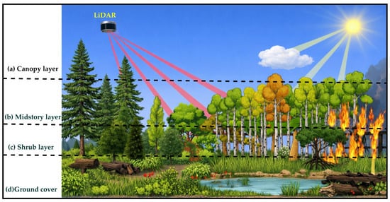
Figure 1. Vertical hierarchy of diverse forest structural part distributions. (a) Canopy layer of emergent trees. (b) Midstory layer of smaller trees. (c) Shrub layers. (d) The forest floor is comprising downed woody debris and litter. The optical and LiDAR principal forest’s vertical stratification is depicted.

To address plant traits and trait variations over time, remote sensing emerged as a widely adopted and cost-effective technique for providing large-scale, long-term, consistent, spatiotemporal, and economically viable scientific information on diverse vegetation biomes [15,16,17]. Consequently, in the past 50 years, low-to-medium-resolution satellite imagery (10–500 m/pixel) has shown great success in driving a wide array of vegetation physiological, anatomical, and geochemical traits at global scales in logistically challenging biomes, e.g., Moderate Resolution Imaging Spectrometer (MODIS) Vegetation Continuous Fields (VCF) products—comprising tree cover, non-tree vegetation, and non-vegetated surfaces, including water—and Landsat time series for AGB [15,18,19]. However, while these systems provide seamless and consistent multispectral (MS) imagery useful for mapping vegetation traits and variations at global scales, they suffer from saturation effects for mapping fine-detailed 3D forest ecosystems [20,21].

High-resolution spaceborne imagery (≈5 m/pixel) and VHR aerial imagery from manned and Unmanned Aerial System (UAS) greatly improved the resolution and representation issues of canopy structural information, e.g., fine-scaled Digital Surface Models (DSMs) [22,23]. Optical remote sensing relies on passive measurements of reflected solar radiation from forest canopies. In mountainous and topographically complex landscapes with dense vegetation, signal interpretation is challenged by terrain-induced illumination variability, canopy self-shadowing, and occlusion effects [24]. Additionally, spectral saturation in high-biomass conditions limits sensitivity to structural and compositional variability, reducing the accuracy of forest attribute retrievals [24,25,26]. The dissemination of sunlight through the canopy to reach the midstory, shrub, and/or ground layer is largely dependent on the structural and physiological characteristics of horizontal and vertical structural complexities of vegetation (Figure 1), and highly dependent on seasonality, e.g., phenological stages—leaf-on and leaf-off conditions [27,28]. In addition, optical remote sensing suffers from occlusions and cloud cover [29]. For example, prairie and savanna ecosystems, largely comprising grasses, shrubs, and plant communities, have been mapped successfully using optical remotely sensed datasets, such as Landsat 30 m data products. On the contrary, dense tropical and boreal ecosystems are challenging to decode the 3D forest structure using optical remote sensing alone [30,31].

To address the forest’s 3D vertical stratification using optical sensed data, the forest’s vertical structural characteristics are established using empirical forest models [26], e.g., the Forest Vegetation Simulator (FVS), to understand growth and yield of forest ecosystems throughout the United States [32,33,34]. FVS simulates 3D forest ecosystems based on forest inventory analysis (FIA) input attributes of field-based observations [33]. Recent findings show that FVS is highly sensitive towards species composition, site index, and tree diameter factor among other parameters [34]. To this end, several studies benchmarked the laser remote sensing (LRS) capabilities in deciphering the 3D forest structural complexities—AGB, forest management practices, forest ecology, and wildland fuel mapping—in wide-area capacity compared with sparsely inputted FVS-based simulations [35,36,37].

Scope and Outline of This Review

Ecological conservation monitoring programs operate at multiple organizational and spatial levels, from species to ecosystems. However, many suffer from a lack of clearly defined goals and hypotheses, as well as weaknesses in survey design, data quality, and statistical power at the onset [38,39]. To this end, many forest structural and functional metrics derived from LRS extend beyond any single application domain, such as forest management [17,40,41]. These metrics are also essential for AGB estimation, fuel mapping, and forest ecology (Figure 2). Consequently, LiDAR datasets within one domain can often play a crucial role across multiple forestry domains [26,42]. Fully realizing LiDAR’s potential in interdisciplinary forest ecosystem research requires a comprehensive understanding of how forest structural, compositional, and functional attributes are intertwined and how LiDAR-derived products can be applied across domains; however, these capabilities remain insufficiently evaluated and utilized [43,44]. Moreover, as LiDAR technology has diversified—yielding an array of commercially viable sensors—a thorough grasp of each sensor’s capabilities, interdisciplinary application scope, and potential future advancements is of paramount importance yet not fully understood [17,37,45].

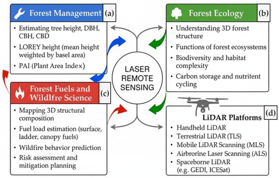
Figure 2. Schematic overview of LiDAR applications across three major forest domains—(a) management, (b) ecology, and (c) wildfire science—and the corresponding (d) LiDAR platforms that enable data acquisition across these themes.

In the light of existing research and review articles addressing LRS of vegetation, this review serves three main objectives: (a) to reinforce the cross-domain applicability of LiDAR-derived a plethora of structural, compositional, functional, and disturbance status indicator forest metrices which are essential for multiple forestry applications [37,42,44]; (b) to identify and synthesize recent technological advancements in LiDAR sensors, operational modalities, and sensor carrier platforms, and to evaluate their demonstrated effectiveness in characterizing forest attributes over large spatial extents [46,47,48]. Moreover, this review highlights the development of multispectral LiDAR (MSL) [49,50], hyperspectral LiDAR systems (HSL) [51], and the integration of LiDAR with optical and Synthetic Aperture Radar (SAR) remote sensing technologies to enhance interdisciplinary investigations of vegetated ecosystems [25,52]. (c) To quantify the forest’s attributes, LiDAR data processing workflows, encompassing both traditional approaches and modern artificial intelligence (AI)-driven techniques [53], with a focus on their practical application in vegetation remote sensing, have been explored [25,54]. Finally, the discussion section provides a brief review of existing reviews and research papers that address the identified knowledge gaps and contribute to one or more application domains of LRS of precision agriculture and precision forestry.

2. Materials and Methods

A comprehensive literature search was conducted on the Web of Science Core Collection (version 5.32) and Scopus to capture peer-reviewed publications from late 1999 through 2025 (n = 619). To improve transparency, search strings combined LiDAR-specific keywords—“space-borne LiDAR (SLS),” ALS, UAS Laser Scanning (ULS), Terrestrial Laser Scanning (TLS), handheld LiDAR, Mobile Laser Scanner (MLS), Simultaneous Localization and Mapping (SLAM), smartphone LiDAR, waveform LiDAR, discrete-return LiDAR, single-photon LiDAR—with ecosystem and application descriptors such as forest*, plantation*, ecosystem*, tropical forest*, dry forest*, wildfire*, fuel mapping*, forest attribute*, and phenotype*. These representative keyword combinations formed the basis of the database queries and ensured broad coverage of vegetation-related LiDAR research. Publications from all major publishers (Elsevier, Springer, Wiley, Taylor & Francis, IEEE, MDPI) were retrieved.

Each record was screened using a simplified PRISMA-style workflow by examining abstracts, figure captions, methodological descriptions, and conclusions to assess relevance. To focus on studies that advanced LiDAR technology or its application in vegetation science, we applied the following inclusion criteria:

• Sensor innovation: New LiDAR hardware or waveform acquisition modes for vegetation remote sensing.
• Platform development: Novel carrier integrations, e.g., multi-sensor or multitemporal deployments of LiDAR sensors.
• Original research: Studies presenting new findings in the LRS of vegetation.
• Processing methods: Development of parametric algorithms or nonparametric (ML/DL) approaches for LiDAR data processing.
• Multi-scale applications: Demonstrations of multitemporal, multiplatform, multispectral, or hyperspectral-LiDAR integration in vegetation contexts

Articles were excluded when they relied solely on established LiDAR data processing frameworks to extract structural attributes without introducing methodological or technological advances or were not directly related to LiDAR applications in precision forestry (n = 285). Statistical distribution analyses and detailed bibliometric assessments were omitted to maintain a focused review of technological development in LiDAR sensor design, platform capabilities, and precision forestry-related applications. Using PRISMA, inclusion and exclusion criteria, as stated above, a total of 334 peer-reviewed articles were included in the present review.

3. Results

3.1. Overview

In the past 20 years or so, LRS has shown great success in deciphering agriculture and forest ecosystems’ structural complexity and diversity in detail, as a stand-alone or through data fusion approaches with multi-source remotely sensed datasets [25,55]. Currently, LiDAR sensors are operational from various carrier platforms, e.g., hand-held sensors, e.g., Simultaneous Localization and Mapping (SLAM) [56], smartphones [57], TLS, MLS, ULS, ALS [58,59,60,61], and SLS, e.g., Ice Cloud and land Elevation Satellite-1 (ICESat-1), ICESat-2 [62], and Global Ecosystem Dynamics Investigation (GEDI) [63], elucidating the vegetation remote sensing by peering through dense forests and deciphering 3D complexities at unprecedented spatiotemporal resolutions [11,64,65,66]. LRS has been widely applied in vegetation studies to quantify forest structural, functional, compositional, and disturbance attributes, e.g., species composition, aboveground biomass, and canopy layering, wildfire science, thereby advancing the understanding of 3D ecosystem functioning, disturbance dynamics, biodiversity, carbon storage, and nutrient cycling [45,65,67,68,69,70,71,72].

3.2. Application Domains

Broadly, LiDAR forest applications can be conceptually grouped into three overarching categories: forest ecosystem research [26,73], forest management and monitoring [74,75], and forest fuels and wildfire science [76,77]. LiDAR datasets collected within one domain are often applicable and can inform analyses across multiple thematic areas (Figure 2). Figure 2a–c illustrate these domains—encompassing management, ecology, and wildfire dynamics—while Figure 2d outlines the LiDAR sensing platforms—terrestrial, airborne, and spaceborne—that enable data acquisition across spatial and temporal scales [31,65,78]. The following sections elaborate on the role of LiDAR within each domain to establish a contextual foundation for this review.

3.2.1. Forest Ecology

The paradigm of the forest ecosystem is rich and dynamic, blue carbon ecosystems (BCE), i.e., mangrove forests [79], tidal marsh ecosystems [80], seagrass meadows [81], dry land ecosystems [82], grassland ecosystems [83], tropical rainforests [84], temperate deciduous [85], temperate coniferous [86], boreal forests [87], tropical montane cloud forests (TMCFs) [72], forest plantations [88], urban forests [89], and savannas, are among the most diverse forest ecosystems globally [90]. The richness and diversity of terrestrial forest ecosystems are not fully understood due to a lack of extensive sampling in 3D space and time [38,78,91].

LiDAR in this respect provides comprehensive mapping covering the state’s entire forest biome with an increasing number of repeated LiDAR surveys decoding the entirety of forest ecosystem structural composition and diversity; for instance, the United States three-dimensional elevation program (3DEP) is one such example for various national and scientific objectives [26,61,68]. In recent studies, LiDAR-based investigations showed that the structural diversity and heterogeneity of terrestrial forest ecosystems promote bird and animal diversity more than single-layer forest canopies [80]. A preponderance of scientific investigation documented the success of the LiDAR datasets originating from various carrier platforms (Figure 2) to provide new insight into forest ecological applications like transpiration [92], microhabitat diversity governs by physical properties of leaves [93], leaf area density (LAD), leaf area index (LAI), canopy cover (CC), canopy closure (CLS), and tree species classification thereby providing 3D attributes of forest environments setting the baseline of “3D ecology” [94,95,96]. For example, a recent study has utilized a novel—the Salford Advanced Laser Canopy Analyzer (SALCA)—dual-wavelength (1063 nm and 1545 nm) TLS to capture species-specific spatial, spectral, and seasonal canopy characteristics, enabling high-resolution assessment of foliage distribution and dynamics beyond the limitations of conventional field surveys [97].

3.2.2. Forest Resource Management

Apart from forest ecosystems investigations (Section 3.2.1), forest resilience and productivity substantially contribute to economic growth, which is assessed through national-level Forest Management Inventories (FMI) [36]. FMIs are subject to the availability of spatially explicit forest structural, compositional, and functional attributes, e.g., DBH, individual tree height ($T_h)$ forest species composition, basal area (BA), stem density, PAI, PAD, and stock volumes [98]. Traditional forest inventories—such as the United States Forest Inventory and Analysis (FIA) program—are effective in delving into forest ecosystems of national significance, yet spatiotemporally constrained to established forest field plots [99,100].

For that reason, extensive wall-to-wall mapping has been accomplished using remotely sensed data to aid FMI’s objectives [65,98,101]. Field data quality, availability, and relevance are subject to the instruments used and the skill of individual surveyors [33,34]. Nevertheless, complex and challenging global and national forest ecosystems’ 3D stratification has not been fully explored to carry out sustainable FMI without integrating multi-sensory remotely sensed datasets at regional and global scales, as witnessed by several publications documenting the success of LiDAR technology in FMI objectives [65]. For example, the role of LiDAR in sustainable forest management [36], operational implementation of a LiDAR inventory in Boreal Ontario [35], and forest age and height mapping using GEDI and ICESat-2 datasets [102]. Despite the operational success of LiDAR in FMI objectives, the application utility of these datasets in forest ecology and wildfire science is not yet fully realized [103,104].

3.2.3. Forest Fuel Structure and Wildfire Hazard Assessment

The paradigm of wildfires globally—and particularly in the United States—has shifted toward more extreme, frequent, and devastating events under the influence of climate change, wildfire suppression, and intensive human intervention in forest ecosystems [105,106]. Wildfires are controlled by four major yet non-linear components, namely Rate of Spread (ROS), Intensity, Flame Length, and Flame Height, which are directly related to fuel load and topography [107]. Broadscale estimation of forest fuel load is therefore critical for wildfire hazard assessment and mitigation, since fuel remains the only fire-related component that can be modified through forest fuel reduction practices, including mechanical thinning, mastication, and prescribed burning [9,11,76,108].

Though wildfires are natural phenomena, and generally they initiate in surface fuelbed, the average physical characteristics of relatively uniform combustible materials define distinct fire environments [108]. Fuelbed organization—its horizontal and vertical continuity—governs fire behavior: surface fuels encompass everything from dead and live herbaceous plants to downed woody debris accumulations of litter, lichen, moss, and duff, while canopy fuels span the understory, middle story, and dominant canopy layers [9,76,109]. Wildfires typically consume surface fuels [9] and transition to crown fires depending on the quantity and continuity of surface and ladder fuels capable of sustaining a flaming front of sufficient height to ignite canopy fuels—namely foliage, and live and dead tree branches [110]. To sustain crown-to-crown wildfire transmission, the canopy fuel loading (CFL)—the combustible fuel available in canopies—plays an important role [111]. Combustible fuel is defined by its chemistry, continuity, and quantity in 3D space and time [112]. Therefore, quantitative estimation requires geometrical representation of the forest’s vertical strata through metrics such as CFL, canopy base height (CBH), and canopy bulk density (CBD) [69,106,112,113,114]. Accurate estimates of these metrics are an essential step towards fire behavior and smoke simulation models, enabling prediction of fire-line intensity, flame height, surface-to-crown wildfires transition, and crown-to-crown propagation, e.g., active crown fire if CBD > 0.10–0.15 kg/m³ [108,112,115].

Spatially explicit metrics such as CBH and CBD can be measured in the field or acquired from NFIs using allometric equations [116,117]. Multiplatform, multispectral, multitemporal LiDAR datasets now enable high-fidelity mapping of both surface and canopy fuels in complex forest landscapes through forest metrics [40,111,118]. Terrestrial LiDAR systems, e.g., TLS, capture fine-scale surface-fuel heterogeneity beneath dense canopies with higher geometric fidelity to estimate canopy and surface fuels through semi-empirical models [118,119,120], while aerial sensors—ULS, ALS, and SLS—provide extensive coverage of canopy fuel metrics and species composition over broad areas [69,121,122,123]. Integrating these platforms yields continuous, high-resolution representations of fuel continuity, heterogeneity, and quantity that exceed those of national fuel products derived primarily from optical remote sensing, e.g., LANDFIRE [121,124,125].

3.3. Structural and Compositional Metrics

To link the forest’s compositional, structural, productivity, and disturbances in interdisciplinary application domains (Section 3.1), quantitative mapping of vegetation structural, compositional, productivity, and disturbance attributes in wide-area capacity is essential [71]—whether for forest ecology, wildland fuel mapping [123], or management applications [52]. These metrics depend on a consistent framework of acronyms, terminology, and precise definitions, as shown in Figure 2. Nevertheless, the naming conventions for forest ecosystem metrics have proliferated and sometimes diverged in subtle ways [14,39,126]. Establishing a unified nomenclature not only provides a clear baseline for advanced studies but also ensures that metrics of canopy architecture, vertical layering, and species composition can be interpreted and compared reliably—particularly when derived from optical and LRS observations [42,127]. Ultimately, an in-depth understanding of the metrics is essential for full utilization in cross-domain application settings [71,104,128]. Therefore, Section 3.2 objectively defines their naming conventions, definitions, and application utility, establishing a baseline for further investigations [129].

3.3.1. Vegetation Cover Fraction (VCF)

VCF or vegetation frictional cover (fCover) is the projection of aboveground vegetation elements, e.g., stems, leaves, and branches, per unit horizontal ground surface [130], as defined in Equation (1). VCF is a dimensionless unit with values of 0 being the lowest (bare ground) and 1 being the highest (dense vegetation cover) for a given area.

$$\mathrm{VCF}={\displaystyle \frac{A_{ground}^{proj}}{A_{ground}}}$$

(1)

where $A_{ground}^{proj}$ is vertically projected vegetation area onto the horizontal plane surface $A_{ground}$ horizontal ground area of the same unit. Green Vegetation Fraction (GVF) and non-photosynthetic vegetation (NPV) are condition-specific components of VCF [131]. NPV and GVF vary when vegetation condition/type is changed and are frictional components of VCF [132,133]. To address the forest’s structural complexity through species-wise distribution, VCF has gained more specific terms and variants, as listed in Table 1.

Table 1. Definitions and applications of fCover-based metrics describing horizontal and vertical vegetation structure across forest strata, from canopy dominance to understory and non-photosynthetic components.

Term	Definition	Application Domain
Effective canopy cover (ECC)	Vertical projection of canopy (overstory) elements per unit horizontal area, excluding small intra-crown gaps [52].	Integrates overstory density and packing, making it a proxy for AGB and productivity; temporal reductions in ECC signal disturbances and structural degradation.
Crown cover (CRC)	Vertical projection of the outer perimeter of all trees’ crowns per unit horizontal area. Small within-crown gaps are ignored. Trees and woody canopies are considered only, and the understory is ignored [134].	Captures broad-scale canopy extent and stand structural stage; decreases in CRC are widely used to quantify disturbance intensity—fire, storms, logging—and associated shifts in canopy dominance.
Specie cover (SPC)	Vertical projection of vegetation elements belonging to a single species per unit horizontal area. Used to estimate species abundance or dominance in mixed stands [135].	Describes species abundance and dominance in space, underpinning species abundance and composition analyses and revealing species-specific responses to disturbance or management.
Stratified Vegetation Cover (SVC)	Vertical projection of vegetation elements belonging to a specific vertical stratum (e.g., overstory, midstory, understory) per unit horizontal area [48,136].	Describes vertical structural complexity and layering, which is a key attribute for habitat heterogeneity and regeneration patterns; highlights how different strata respond to canopy gaps and disturbance regimes.
NPV cover (NPVC)	Vertical projection of non-photosynthetic vegetation (NPV, e.g., senescent, woody, or dead vegetation) per unit horizontal area [137].	Acts as a sensitive indicator of mortality, fuel build-up, and post-disturbance trajectories, and is increasingly used to monitor vegetation condition and fire-related fuel dynamics at landscape scales.
Canopy closure (CLS)	The proportion of the sky hemisphere (180° field of view) obscured by vegetation when viewed from a single point beneath the canopy [138].	Controls understory light and microclimate, thereby regulating regeneration and understory composition; sharp declines in CLS reflect gap formation and canopy removal from disturbances.
Canopy fraction (CF)	The proportion of incident radiation intercepted by canopy elements along a specific viewing or illumination direction (directional fCover) [139].	Closely linked to fPAR and canopy photosynthesis, so it is a key predictor of productivity and carbon uptake, and can detect changes in functional foliage following stress or disturbance.

Despite the clear definitions of VCF and its variants (Table 1), most image-segmentation approaches of optical remotely sensed data still struggle to separate GVF from heterogeneous backgrounds comprising litter, understory (GVF and NPV), soil, and sky due to spectral variability, uneven illumination, and complex background composition [140,141]. Although ground-based digital photography and UAV imagery (typically 1–5 cm pixel size) can retrieve different variants of fCover with reasonable accuracy, performance declines sharply under shadow effects, specular reflection, or mixed pixels in heterogeneous canopies, which requires extensive calibration and harmonization with other sensors [16,142]. Consequently, optical methods alone are challenging to produce consistent fCover estimates across diverse illumination, canopy structural complexity, and view-angle effects [142,143]. LiDAR relieves many of these limitations by directly capturing the 3D spatial distribution of vegetation elements at submeter to centimeter (cm) resolution [45,48,143]. ALS~0.5–2 m, provides landscape-scale estimates of canopy and subcanopy structure; ULS~2–10 cm, resolves fine-scale crown geometry; TLS~1–5 mm, characterizes foliage, branches, and within-crown gaps; and MLS is capable of capturing fine-resolution forest understory and forest floor [114,144,145,146].

However, single-wavelength LiDAR (e.g., 1064 nm) alone does not capture spectral properties or photosynthetic status, making it complementary to optical and SAR observations [104]. Integrating LiDAR-derived structural metrics with optical VCF products and SAR observations that are sensitive to canopy volume and moisture conditions supports a more comprehensive and physically consistent characterization of vegetation cover, canopy architecture, and disturbance processes across spatial scales [40,62,147]. As emerging modalities, MSL and HSL have the potential to improve, e.g., GVF and NPV characterization using LRS by jointly capturing 3D structural information and reflectance properties [49,148], which is currently obtained through data fusion with optical multispectral and hyperspectral datasets [47].

3.3.2. Stand Structural Metrics

Measurable ecosystem indicators are needed for the scale and purpose at which forest ecosystems are being studied—forest ecology, forest management, and fire behavior modeling [134,149]. Forest ecosystem metrics are placed into two broad categories: the identification of key species-related structural metrics for area-based estimates [103], e.g., stand-level structural complexity [111]; and more specific individual-tree-level structural estimates [150]—as shown in Table 2. Stand-based structural attributes are instrumental in terms of understanding ecosystem functionality, forest management practices, and wildfire fuel loadings [110]. However, the structural complexity of individual trees necessitates segmentation and classification at the plant or organ level (e.g., stem, branches, and foliage), making LiDAR instrumental for resolving 3D tree architecture [110,111]. A list of widely used tree/stand structural attributes is summarized in Table 2.

Table 2. Structural and functional attributes used to quantify three-dimensional tree and canopy complexity, spanning stem geometry, height structure, foliage organization, AGB cross-domain, and canopy fuel properties relevant to ecosystem functioning, disturbance, and fire behavior.

Term	Definition	Application Domain
Diameter at Breast Height (DBH)	The diameter of a tree stem measured at 1.3 m above the ground on the uphill side, expressed in (cm) [151].	Core variable for tree allometry, AGB estimation, growth trends, and size-class structure analyses across forest types.
Quadratic Mean DBH (QMDBH)	A stand-level diameter representing the mean trees’ BA, calculated as $\mathrm{QMDBH} = \sqrt{\left(\sum \left({\mathrm{D}\mathrm{B}\mathrm{H}}_{\mathrm{i}}^2\right)/\mathrm{N}\right)}$, where DBHi is the diameter (cm) of the ith tree, and N is the number of trees. QMD gives greater weight to larger trees [152].	Particularly useful for tracking dominance of large trees, assessing stand maturity, and identifying structural transitions relevant to productivity and resilience.
Mean Tree Height (Th)	The arithmetic mean height (m) of the 100 trees ha−1 with the largest DBH values; commonly referred to as dominant height [147].	Serves as a sensitive indicator of site productivity and successional advancement, widely used to compare stand vigor and evaluate disturbance recovery trajectories.
Average Height	The mean height (m) of all live trees within the plot having DBH ≥ 9.1 cm [147].	Calibrates height–diameter models and aids in assessing stand uniformity and regeneration success.
Tree (Stem) Density	The number of live, healthy stems per hectare (stems ha−1) with DBH ≥ 9.1 cm [153].	Vital for measuring competition, stand crowding, regeneration dynamics, density-dependent mortality, as well as assessing the effects of thinning or management practices.
Basal Area (BA)	The total cross-sectional area of tree stems at 1.3 m above ground height per hectare (m2 ha−1), computed as BA = (π/4) × Σ ((DBHi/100)2), where DBHi is in centimeters converted to meters for area calculation [154].	Highly informative for quantifying stand stocking, competition intensity, and potential carbon sequestration, while revealing structural responses to thinning or disturbance.
Gross Merchantable Volume (GMV)	The sum of all merchantable stem volumes (m3 ha−1), excluding bark, branches, and foliage, calculated from DBH–height relationships or taper equations [35].	Supports wood-resource planning, but also reflects structural development and disturbance impacts through changes in merchantable stem availability.
Aboveground Biomass (AGB)	The total dry mass of all aboveground tree components (stem, bark, branches, leaves) per unit area (Mg ha−1). Estimated as AGBi = a × (DBHi)b × (Hi)c × ρi, where a, b, and c are empirical coefficients, Hi is tree height (m), and ρi is wood density (g cm−3) [155]. There are many variants of AGB equations, and herein we used the one that provides more accurate estimates, e.g., when tree height is included in the modeling—as opposed to another variant that is only based on DBH [156].	AGB is a key metric for ecosystem carbon accounting and productivity monitoring, and it enables robust comparisons of disturbance severity, recovery trajectories, and fuel conditions across forest stands. Moreover, AGB plays a central role in cross-domain applications, supporting integrated assessments of forest ecology, wildfire dynamics, productivity, and wildfire smoke emissions through analyses of pre- and post-fire biomass change [157].
Leaf Area Index (LAI)	LAI is the one-sided green leaf area per unit horizontal ground area (m2 m−2), a dimensionless measure of canopy density and light interception. Defined as LAI = ∫0H LAD(z) dz, LAD(z) = (m2 m−3), and H = canopy height (m). Alternatively, LAI = −(cos θ/G(θ)) ln P(θ), where θ = zenith angle (rad), G(θ) = projection function (dimensionless), and P(θ) = gap fraction (dimensionless) [96].	Integrates canopy greenness and light-use capacity, enabling assessment of photosynthetic potential, drought impacts, and canopy thinning due to natural or anthropogenic disturbance.
Leaf Mass per Area (LMA)	The ratio of dry leaf mass to one-sided leaf area, LMA = Mᴸ/Aᴸ, where Mᴸ is leaf dry mass (g; oven-dried 65 °C for 48 h) and Aᴸ is leaf area (m2). Units = g m−2 [67].	Indicates functional traits linked to species strategies and physiological stress, aiding interpretation of canopy condition, resource allocation, and structural acclimation.
Specific Leaf Area (SLA)	The inverse of LMA, SLA = Aᴸ/Mᴸ, representing leaf area per unit dry mass (m2 g−1); an indicator of photosynthetic potential [158].	It enables the identification of species’ growth strategies and canopy effectiveness and assists in assessing how stress affects leaf structure or productivity.
Leaf angle Distribution (LAD)	LAD describes the statistical distribution of leaf inclination angles (0° = horizontal; 90° = vertical), representing three-dimensional leaf orientation in the canopy [146]. It satisfies ${\int }_0^{\pi /2}f\left({\theta }_l\right) d{\theta }_l = 1;$ and defines $G\left({\theta }_i\right)= {\int }_0^{{\displaystyle \frac{\pi }{2}}}f\left({\theta }_l\right)\cos \left({\theta }_l\right)\left|\cos \left({\theta }_i - {\theta }_l\right)\right| d{\theta }_l,$ where f(θl) = probability density of leaf inclination angle (rad−1), θl = leaf inclination angle (rad), θi = incidence angle (rad), and G(θi) = projection function (dimensionless).	Shapes the directional interception of light and energy throughout the canopy and is essential for interpreting optical and LiDAR radiative signals; together with vLAD, it informs how foliage is arranged both angularly and vertically, linking canopy geometry to reflectance, photosynthesis, and disturbance responses.
Vertical Leaf Area Distribution (vLAD)	vLAD is the one-sided leaf area per unit canopy volume (m2 m−3), defined as vLAD = Aᴸ/Vc, where Aᴸ = leaf area (m2), Vc = canopy volume (m3). It can be expressed as vLAD(z) = −(1/G(θ)) (d/dz) ln P(z) and integrates vertically as LAI = ∫0H vLAD(z) dz, where vLAD(z) = vertical leaf area density (m2 m−3), P(z) = gap fraction (dimensionless), G(θ) = projection function (dimensionless), H = canopy height (m) [159].	Describes the vertical allocation of foliage and provides a structural counterpart to LAD, together revealing how canopy orientation and layering jointly regulate light penetration, photosynthetic gradients, and vertical reorganization following disturbance or succession.
Canopy Gap Fraction (CGF)	The probability that a beam of light passes through the canopy without intersecting vegetation, CGF = CGF(θ) = exp(${\displaystyle \raisebox{1ex}{$-G\left(\theta \right)LAI$}\!\left/ \!\raisebox{-1ex}{$\cos \theta $}\right.}$), where G(θ) is the projection function at zenith angle θ [158].	Highlights canopy openness and understory light availability, serving as an indicator of disturbance-driven gap formation and canopy regeneration.
Plant Area Index (PAI)	The total one-sided area of all aboveground plant elements (leaves, branches, and stems) per unit ground area (m2 m−2). Includes both GVF and NPV components [158].	Captures total plant surface area influencing radiative transfer, productivity, and habitat structure, and is useful for understanding both canopy packing and disturbance effects.
Plant Area Density (PAD)	The total one-sided plant area per unit canopy volume, PAD = PAI/Hc, where Hc is canopy height (m); expressed in m2 m−3 [159].	Used to characterize vertical vegetation packing, within-canopy flow and turbulence, and structural fuel continuity.
Canopy Bulk Density (CBD)	The mass of canopy fuels (foliage + fine twigs) per unit canopy volume, CBD = Mc/Vc, where Mc is canopy fuel mass (kg), and Vc is canopy volume (m3). Units = kg m−3 [124].	Determines crown-fire propagation potential and provides a structural measure of canopy continuity sensitive to thinning, mortality, and other disturbance processes.
Canopy Base Height (CBH)	The lowest height above ground (m) where sufficient live or dead canopy fuel exists to sustain upward flame propagation; corresponds to the base of continuous crown fuel [124].	Reflects vertical fuel continuity and crown-fire initiation risk, and signals structural changes tied to management, mortality, or ladder-fuel development.
Lorey’s Height (Hᴸ)	The basal-area-weighted mean height of all trees, Hᴸ = Σ (hi × bai)/Σ(bai), where hi is tree height (m), and bai is basal area (m2) of ith tree [160].	Weighed by dominant trees, it conveys stand productivity and structural complexity and responds strongly to thinning, competition, and post-disturbance regeneration.
Canopy Fuel Load (CFL)	The total dry mass of canopy fuels (foliage + fine branches) per unit ground area, CFL = Mc/AG, where Mc is canopy fuel mass (kg), and AG is ground area (m2); expressed as kg m−2 or Mg ha−1 [40,124].	Quantifies canopy fuel available for combustion, aiding in fire-severity prediction and assessment of AGB redistribution following disturbance or management.
Available Canopy Fuel (ACL)	ACL (sometimes “Available Canopy Fuel Load,” ACFL) refers to the portion of canopy fuel that is consumed or participates in active crown fire propagation under given moisture and heat conditions. ACL = f × CFL, where f is an empirical availability factor (often 0.3–0.5 depending on forest type and fuel moisture) [124].	Represents the combustible canopy mass and complements CFL and CBD by emphasizing fuel availability rather than total fuel quantity; changes in ACL highlight shifts in canopy dryness, ladder-fuel structure, and disturbance-driven modification of fire behavior potential.
Foliage Height Diversity (FHD)	FHD is an information-theoretic index quantifying the vertical heterogeneity and evenness of foliage distribution across canopy height strata. It represents the vertical component of overall forest structural diversity. FHD is calculated using Shannon’s entropy as follows: $FHD = - \sum {p_{\mathrm{i}} ln \left(p_{\mathrm{i}}\right)}_{i = 1}^n$, where pi = proportion of total foliage area in layer i (dimensionless), and n = number of vertical canopy layers (unitless). Higher FHD indicates greater vertical complexity and canopy stratification [31,39].	Captures vertical stratification of foliage and informs habitat complexity, structural evenness, and species niches; compared with FSD, FHD isolates the vertical dimension and is particularly sensitive to disturbance processes that alter canopy layering without affecting horizontal variability.
Forest Structural Diversity (FSD)	FSD is a multidimensional measure describing the variability and complexity of forest structure, encompassing both vertical (e.g., canopy layering, foliage height diversity) and horizontal (e.g., tree size, crown geometry, gap distribution) attributes. It is commonly expressed as a composite function of multiple structural metrics: $FSD = f \left( FHD, {CV}_h, {Var}_{crown}, {Gap}_{index}, {Stem}_{density} \right)$, where CVh = coefficient of variation in canopy height (horizontal variability), Var(crown) = variance in crown shape or volume, Gap index = heterogeneity of canopy openings, and Stem density = spatial variability of tree stems [161].	Integrates both vertical (e.g., FHD) and horizontal (e.g., crown variability, gap patterns) dimensions of complexity, offering a more holistic representation of ecosystem structure; its contrast with FHD highlights how disturbance can differentially affect vertical layering versus horizontal heterogeneity.

Together, the metrics in Table 1 and Table 2 provide a structured basis for quantifying forest composition, structural diversity, and disturbance status across local-to-global scales [9,66,74]. In general, size- and stocking-related attributes, e.g., DBH, $T_h$, and AGB, are primarily driven by tree dimensions and wood properties, whereas canopy-functional and vertical-organizational attributes, e.g., LAD and vLAD, reflect foliage quantity, spatiotemporal arrangement over time, and within-canopy light environment—properties that are difficult to characterize comprehensively using traditional FFI surveys alone and are often mapped or scaled using remotely sensed datasets [26,58,65,162]. LRS has proven highly effective for deriving these metrics, providing detailed vertical stratifications at different scales and resolutions—with substantially greater fidelity than optical datasets [31,40,96,113,124]. While CBH, CBD, and CFL are routinely applied in wildfire risk assessment [54,123], other LiDAR-derived structural metrics, such as FHD, LAD, and FSD, remain underexplored in fire behavior research [161], yet are commonly used in forest ecology and biodiversity research despite their potential relevance to wildfire behavior. This gap highlights opportunities for broader cross-domain applications of forest structural metrics (Table 1 and Table 2).

It should be noted that the metrics listed in Table 1 and Table 2 provide fundamental and widely used forest structural and functional attributes [31]. A wide range of derivative attributes—many of which build directly upon these core metrics—can be found in the literature to further delve into forest ecology, forest management, and wildland fuel management practices [163]. As one example, the book “Forest Stand Dynamics” offers a mechanistic understanding of forest growth and stand development that helps silviculturists, forest managers, and ecologists design site-specific treatments balancing timber production, biodiversity, and ecosystem resilience under increasing multi-use demands [39,164].

Table 1 and Table 2 summarize the core role of LRS in understanding forest ecosystems. Section 4 reviews the evolution of LRS, sensor types, and carrier platforms, providing the foundation for understanding how LRS enables the retrieval of the structural attributes across multiple forest scales.

4. Advances in LiDAR Sensors and Carrier Platforms

An ever-increasing technological advancement in laser, Inertial Measurement Unit (IMU), and Global Navigational Satellite System (GNSS) sensors, along with static, mobile, aerial, and SLS platforms, efficient data storage and processing units, led the development of an unprecedented wide array of LiDAR sensors [33,34,35,36].

4.1. Light Detection and Ranging: Conceptual Framework

A LiDAR unit is an integration of laser(s), receiver optics, and a timing unit, along with IMU/INS and GNSS (Figure 3) [165,166]. A precise internal timing unit records the time lapse between the outgoing laser pulse and backscattered laser echoes received at the sensor’s receiver–detector (Figure 3a,b) to calculate the range of the target objects. The range of target objects is calculated using two widely used methods: time of flight (TOF), the time taken by an emitted laser echo to return from target objects, and the phase-shift (PS) method [167], in which the transmitted and received laser echoes are superimposed to calculate the phase-shifts, providing the range of the targets [168]. The oscillating mirror is used to cover a FOV, i.e., a maximum area that can be seen by a laser scanner (Figure 3d). The instantaneous (IFOV) is an individual laser footprint that depends on laser beam divergence (Figure 3c), i.e., laser light spreads as it moves through the atmosphere and is measured in milliradians (mrad). The beam divergence depends on several factors, such as atmospheric conditions and distance from the target. For instance, LiDAR casts a larger IFOV when atmospheric conditions deteriorate or when target distance increases; consequently, SLS platforms like ICESat-2 produce a 14 m diameter laser footprint, while airborne LiDAR yields a footprint of about 30 cm. Moreover, beam divergence is characteristic of spectral wavelengths at which laser echo is being transmitted, i.e., lasers emitted at different wavelengths have varying degrees of beam divergence [169]. Understanding these critical differences in LiDAR sensors’ physical concepts is essential to quantify the forest ecosystems in a multi-sensory conundrum [162].

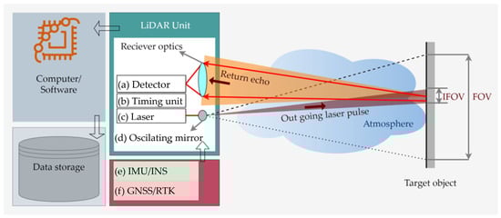
Figure 3. Schematic illustration of the principal functioning of a LiDAR system. The LiDAR unit consists of (a) a detector, (b) a timing unit, (c) a laser source, (d) an oscillating mirror, (e) an IMU/INS, and (f) a GNSS/RTK unit. The outgoing laser pulse is transmitted toward the target, and the returned echo is received by the detector. The recorded signals are processed by the onboard computer/software and subsequently stored in the data storage unit.

4.2. LiDAR Modalities

With recent advances in multifacet technological advances in sensor optics, LiDAR sensors purely from an operational perspective can be broadly classified into two main categories: linear-mode LiDAR and photon-counting LiDAR (PCL) systems [170,171]; since MSL and HSL are based on the same operational techniques with several wavelengths, they fall within these two broad classes [172,173,174]. LiDAR modalities are distinguished by the sensitivity of their objectively designed receiver optics, which determine how reflected laser echoes are treated by the receiver optics, as shown in Figure 4. The higher the sensitivity of the receiver optics, the weaker the signal they can detect [175]. Linear-mode LiDAR systems are further subdivided into two types: discrete-return and waveform [175].

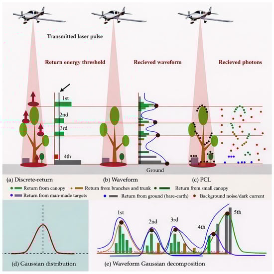
Figure 4. Illustration of LiDAR modalities. (a) Linear-mode discrete-return. (b) Linear-mode waveform. (c) Photon Counting LiDAR (PCL). (d) Gaussian function for the energy distribution of a laser spot. (e) Gaussian decomposition of LiDAR waveforms to resolve different reflecting surfaces within the footprint of backscatter laser echoes.

4.2.1. Discrete Return

The discrete-return systems record the backscatter laser echoes that meet the receiver’s energy sensitivity threshold [64]—see Figure 4a. Discrete returns are a gated system—only significant returns are allowed through the receiver optics. For example, the portion of energy reflected from the top of the canopy or bare ground is recorded as the first, second, and/or third return from the middle canopies, and fourth return from the understory—shrubs or the ground [61]. Most discrete-return systems provide three or more returns, presenting the simplest geometry of terrestrial objects. Discrete return produces a 3D cloud of point measurements referred to as a “point cloud” [175]. Over the past two decades, discrete return has been the most widely used linear-mode system, resulting in massive point clouds of forest ecosystems [18,65,150,162]. The initial development of discrete-return systems offered easier onboard data storage, processing, and analysis—addressing technological constraints at a time when massive data processing and storage were computationally challenging [61]. In addition, point densities, i.e., total number of returns from a unit area/m², were in the range of 1 to 1.5 points (pts)/m² [176]. In recent times, discrete-return systems have undergone significant development in terms of onboard data storage, near-real-time data processing, and receiver optics [61,177]. Hence, massive data collection is possible with significantly higher point densities. Modern, discrete-return systems can register more than 10 returns with point densities ranging from 5 to 360 pts/m², originating from terrestrial and aerial platforms [94,176,178].

4.2.2. Waveform LiDAR

Waveform systems known as full-waveform laser scanning [64] are capable of registering entire backscattered signals with a much higher sensitivity of receiver optics [179]—see Figure 4b. Consequently, waveform LiDAR presents richer information on vertical vegetation structural complexity than discrete-return systems [180,181].

To extract information from the waveform, Gaussian decomposition is performed to process the waveform into meaningful observations of terrestrial objects [182]—see Figure 4d,e. Waveform processing is a complex task that generally requires advanced signal processing pipelines to extract useful information about reflecting surfaces within the laser footprint, such as Gaussian decomposition [183]. The prerequisite of Gaussian decomposition is to define the number of fitting curves as a function of waveform data processing, i.e., to determine the total number of reflecting surfaces to be resolved (Figure 4e). Over the simplified surfaces, e.g., flat ground, a single surface can be resolved by fitting a single Gaussian curve, yet over complex surfaces, e.g., forest ecosystems, resolving all the reflecting surfaces within the laser footprint becomes challenging when several reflecting surfaces are unknown, or reflectance from different surfaces is diffused [64]—see Figure 4e. Recent advances in LiDAR waveform decomposition include Linearly Approximated Iterative Gaussian Decomposition (LAIGD) [183], which iteratively detects weak laser echoes in complex waveforms; Bayesian decomposition [184], where waveform parameters are estimated within probabilistic frameworks; B-spline and particle swarm optimization [185]. Furthermore, the Fuzzy Mean-Shift approach [186], Gaussian mixture model [187] and DL approaches can resolve individual and defused reflecting surfaces from single-wavelength or MLS/HSL data [188,189,190]. In recent times, with computationally efficient systems, e.g., cloud computing, waveform LiDAR and advanced waveform decomposition methods have become increasingly popular in forest ecosystem studies [97,181,191,192,193,194].

4.2.3. Photon Counting LiDAR

The PCL is an advanced LiDAR modality [195]. Unlike linear mode systems—such as discrete-return and waveform—the PCL technology is sensitive at the photon level, i.e., each photon reflected within the FOV of the sensor is recorded by the single photon detectors (SPDs) and counted as a valid observation, thereby making it capable of recording 1000 s of returns to construct very high-density point clouds [153,196]—see Figure 4c. Photon-level sensitivity enables PCL systems to operate with reduced power at higher altitudes than linear mode systems, e.g., ICESat-2 [193]. Conversely, at photon-level sensitivity, background noise photons are introduced, originating from sunlight of the same spectral wavelength or sensor thermal radiation—specifically dark current—as illustrated by red dots in Figure 4c. Figure 4c indicates that the signal photons are more clustered, and noise photons are randomly distributed, making noise-photon seclusion conceivable. Thanks to advanced noise filtering algorithms, a large share of the noise photons is removed algorithmically from final deliverables [196,197]. Currently, PCL systems are operational at 1550 nm and 532 nm, given that PCL technology is mature at these wavelengths; an example is ICESat-2 [198]. The PCL with much higher point densities can capture forest structural complexities in more detail than its counterpart’s linear mode LiDAR systems [174,175]. PCL systems are viewed as the next-generation LiDAR for high-resolution forest ecosystem studies [195,199].

4.3. Carrier Platforms

The choice of a LiDAR sensor modality (see Section 4.2) and carrier platform is influenced by several critical factors, including the characteristics of the operational environment, the scale and extent of the area to be mapped, logistics feasibility, and the integration with sister technologies—specifically IMUs and GNSS [200]. These diverse requirements have driven substantial advances in both LiDAR sensors (Section 4.2) and their carrier platforms over the past two decades [61,177]. This section provides a detailed overview of LiDAR sensors based on key aspects: (a) carrier platforms, (b) their payload capacities, (c) data quality and integrity, (d) spatiotemporal resolution, and (e) challenges in geometrical representation (Figure 5).

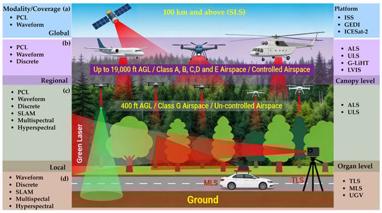
Figure 5. Stratification of LiDAR sensor platforms by spatial coverage, acquisition mode, and operating altitude. (a) Spaceborne LiDAR systems (SLS), operating at orbital altitudes (≥~100 km above mean sea level), employ PCL or full-waveform techniques with meter-scale laser footprints to provide global observations (e.g., GEDI, ICESat-2). (b) Airborne LiDAR systems (ALS) deployed from crewed aircraft operate from approximately 120 m to 5800 m above ground level (AGL) within controlled airspace, supporting discrete-return, full-waveform, and photon-counting modalities with footprints ranging from centimeters (cm) to several meters (m), e.g., NASA’s Goddard LiDAR, Hyperspectral and Thermal Imager (G-LiHT), and the Land Vegetation and Ice Sensor (LVIS). (c) Low-altitude airborne and uncrewed systems, including commercial ALS and UAS LiDAR systems (ULS), operate below~120 m AGL (often in uncontrolled airspace), enabling high-resolution canopy-level measurements with high pulse repetition frequencies. (d) TLS and MLS, mounted on ground-based, e.g., Uncrewed Ground Vehicles (UGV) or crewed vehicle platforms, acquire ultra-dense point clouds at the organ and surface-fuel scale, supporting detailed characterization of stems, branches, and understory vegetation.

4.3.1. Terrestrial Laser Scanning

The term TLS is used when a LiDAR is operated in static mode, i.e., LiDAR unit(s) mounted over a fixed platform, e.g., crane, tower, gantry, and/or tripod. Currently, TLS is operational in linear modes, specifically discrete-return and waveform [64,97,167,201]. TLS systems are primarily mounted on tripods with 360-degree scanning configurations in circular patterns [202]. Unlike ALS (Figure 6c–f) and ULS (Figure 6b–e) scanning vegetated landscapes from nadir and off-nadir positions, the occlusions caused by branches, stems, and leaves are less pronounced in TLS point clouds [58,68]—see Figure 6a. However, the occlusion effect prevails with increasing distances from the scanner location; object(s) near the scan station occlude the far objects [126,203]. To cover a larger geographic extent and mitigate the occlusion effect, several TLS stations are analytically distributed throughout the study area, and point clouds originating from TLS stations are registered [58,204]. Point cloud registration is analogous to the georeferencing of satellite imagery to a single geographic coordinate system. In natural landscapes (see Figure 6), finding the conjugate points, i.e., common reference points in point clouds originating from two different TLS stations, is a challenging task. Alternatively, co-registration is achieved using 12–18 retroreflective targets as control points and marker-free registration approaches [204]. TLSs integrated with GNSS can help to align TLS stations automatically. In a multiplatform conundrum (Figure 6), point clouds originating from aerial platforms—such as ALS and ULS—are required to be registered with concurrent TLS point clouds to obtain a detailed geometric representation of forest landscapes [203,205,206]. Under dense canopies, TLS captures the understory in more detail than its counterparts, ALS or ULS, and vice versa [68,202,207]. However, the placement of TLS stations (Figure 6) requires theoretical and practical considerations—such as sensor type, range, scanning configurations—for TLS surveys in diverse forest environments to obtain canopy structural details [208].

TLS—such as the Leica ScanStation—can capture up to 50,000 pts/s, with a maximum range of 134 m at~18% surface reflectance, and a narrow beam divergence of 0.14 mrad, operating at the visible portion of the electromagnetic spectrum (532 nm). The term 18% reflectance means that only 18% of the incident laser beam energy is reflected from the target object(s); the remaining 82% is either transmitted, reflected away from the sensor FOV, or absorbed by the target object(s) [209]. Figure 6a demonstrates TLS-based extensive geometric representation of shrubs and trees’ woody parts, stems, branches, and non-woody leaves, which are essential for extracting forest structural attributes, e.g., DBH, tree height, stem density, PAI, LAI, and LAD [210]. TLS provides a time-series 3D representation of the forest’s vertical strata at a given locale, offering critical insights into the forest ecosystem’s function and its response to physical changes driven by climate change [13,146,211]. To scale up 3D vertical stratification from a locale to landscape level, TLS has extensively been used in conjunction with other carrier platforms—such as ULS and ALS (Figure 6)—and backpack laser scanners (BLS). A LiDAR unit in backpack configuration, carried by a human through forests, is generally useful to compensate for the occlusion effects of TLS [100,212]. Some recent reviews addressing the TLS applications in forestry, e.g., segregating tree wood–leaf components [213], an international TLS network for advancing 3D ecological insights into global tree systems [202], and expanding the horizon of TLS in forest ecology, are the most significant contributions extending the knowledge on TLS applications [100,146].

Figure 6. Comparison of different LiDAR platforms for concurrent single surveys. (a–c) Side-view cross-sections (40 m transect, blue line in (d)) illustrating vertical canopy stratification, with point colors representing elevation above ground. (a) TLS captures detailed lower-canopy, stem, and understory structure but is affected by occlusion in the upper canopy. (b) ULS provides improved sampling of mid- and upper-canopy layers while partially resolving understory structure. (c) ALS primarily samples the upper canopy and ground surface, with limited representation of understory elements. (d–f) Plan-view representations of point-cloud density and sampling geometry for (d) TLS, (e) ULS, and (f) ALS, highlighting platform-dependent area-coverage in a single survey (black arrows). The concurrent open-source TLS, ULS, and ALS datasets were provided by Weiser et al. (2022) [214].

Figure 6. Comparison of different LiDAR platforms for concurrent single surveys. (a–c) Side-view cross-sections (40 m transect, blue line in (d)) illustrating vertical canopy stratification, with point colors representing elevation above ground. (a) TLS captures detailed lower-canopy, stem, and understory structure but is affected by occlusion in the upper canopy. (b) ULS provides improved sampling of mid- and upper-canopy layers while partially resolving understory structure. (c) ALS primarily samples the upper canopy and ground surface, with limited representation of understory elements. (d–f) Plan-view representations of point-cloud density and sampling geometry for (d) TLS, (e) ULS, and (f) ALS, highlighting platform-dependent area-coverage in a single survey (black arrows). The concurrent open-source TLS, ULS, and ALS datasets were provided by Weiser et al. (2022) [214].

4.3.2. Mobile Laser Scanning

When a LiDAR is mounted on a moving platform—e.g., crewed or uncrewed UGV, a boat, or a robot—it is referred to as an MLS system. Moreover, hand-held MLS (HMLS) and BLS are also considered as MLS [151]. MLS systems integrate several sub-systems: laser unit(s), IMU(s), GNSS, and a control unit/onboard computer that operates all subsystems, synchronizes/integrates their measurements (Figure 3), data storage, near-real-time onboard data processing, and visualization [60,215].

Compared with their counterpart TLS (Figure 6a–d), MLS provides continuous coverage along the carrier platform’s trajectory [215,216]. The geometric complexity and positional accuracies of TLS and MLS are within millimeters (mm), given that LiDAR sensors are integrated with high-precision IMUs and GNSS. MLS is at the forefront of urban forestry—an emerging topic in modern cities and zero-emission ecosystems—combating climate change [217]. However, under the dense forest canopy, GNSS positioning could be challenging due to signal obstruction, compromising the positional accuracy of MLS [166]. Classical MLS, e.g., mounted on vehicles, is challenging to deploy in complex forest ecosystems; however, collecting time-series LiDAR data along roads venturing through the forest landscape provides an opportunistic window that has been successfully used for MLS applications [216]. Given the surveying challenges of complex forest landscapes, MLS is more favorable in urban forestry [217,218], while MLS systems in conjunction with TLS are more feasible in complex forested landscapes [100,119]. SLAM is also classified as an MLS system [217]. Given that the SLAM system is based on LiDAR sensors, the counterpart photogrammetry-based SLAM systems are also available, which can effectively overcome the issues of GNSS-based position errors [56,166]. “Multiplatform MLS: Usability and Performance” is an interesting read on different MLS carrier platforms and their applications in natural and urban environments [60].

4.3.3. UAS Laser Scanning

Unoccupied Aerial Vehicle (UAV) or UAS or Remote Piloted Aerial System (RPAS) are the acronyms used for any aerial platform controlled by a remote pilot in command (PIC), including tether systems, i.e., a permanent physical link through wire/cable to UAS flying above the ground, offering an unobstructed aerial view of large forested landscapes [122,212,219]—see Figure 6b–e. Moreover, in the context of acronyms used to describe LiDAR sensors onboard remotely controlled aerial platforms, acronyms such as UAS-LiDAR [220] and drone LiDAR systems (DLS) are also used [221]. In this article, we use the acronym “ULS,” which is more consistent with other laser scanning acronyms used, e.g., MLS, and ALS [61,215].

In recent times, UAS technology has significantly matured with more endurance, longer duration, autonomous flights, maneuverability, obstacle avoidance, and terrain following, with increased maximum take-off weight (MTOW), and vertical take-off and landing (VTOL) capabilities [222]. High level of miniaturization of onboard computers, GNSS, INS, receivers, and antennas, i.e., integration of subsystems to a hybrid measurement unit (HMU), enables ULS operations in real time with cm-level positional accuracies [223,224]. Therefore, ULS are more versatile and easier to use for Photogrammetry and Remote Sensing (PaRS) applications over desired areas with multiple payload capabilities—including multispectral, hyperspectral, and thermal sensors [219,223,225]. ULS offers the added advantage of reduced operational costs, fuel, total crew members, and controlled-space clearance—a requirement for ALS [143,226]. Moreover, ULS allows faster data collection and pre-/post-processing than ALS [227]. On the contrary, UAS are allowed in uncontrolled space (G, see Figure 5c) with a maximum altitude of 450 ft AGL and MTOW of 25 kg in the U.S., with a valid UAS pilot license [143]. Similar restrictions are applicable in many other countries. Such restrictions limit the ULS data collection over wide areas compared with ALS [228,229].

TLS and MLS—operational from the ground—pose navigational and logistical challenges in complex forest ecosystems [122]. Given the added advantage of aerial platforms, ULS has recently become more popular for LiDAR data collection over larger areas than their counterpart, TLS and MLS, capturing similar geometric complexities of forest ecosystems (Figure 6). With off-nadir pointing and different flight directions, occlusion effects were found to be lessened under dense forest canopies [59,226,230].

4.3.4. Airborne Laser Scanning

${ALS}_{FW}$, and ${ALS}_D$ systems have been operational since 1999 and are the leading technique for LiDAR data collection over a larger extent, in a wall-to-wall mapping configuration [65]—see Figure 6c–f. ALS have been deployed using various LiDAR modalities, including discrete, waveform, PCL, MSL, and HSL [61,174,177]. ALS, onboard crewed aircraft with MTOW several fold higher than ULS, is capable of covering much larger areas in a single flight [231]. The widespread adoption of ALS can be attributed to its operational maturity and development spanning over two decades (Figure 6c–f). ALS are employed at state or national scales, delivering high-resolution topographic data, e.g., the 3DEP program [18,65]. The extensive use of ALS is evidenced by numerous LiDAR-related publications, highlighting its success and reliability [18,150,174,232].

ALS are flown by commercial operators with funding from research institutions or the government to acquire LiDAR datasets over wide areas, generally covering hundreds of km² [65]. In developed countries, e.g., the United States, national-level ALS data are currently available for research and natural resource management [233]. Though multitemporal or bi-temporal (a site surveyed twice) are only available over certain ecological regions in the U.S. and other developed countries, e.g., Europe and Oceania [96,234]. ALS surveys covering an entire country are costly, time-intensive, and may take years to complete. For example, USGS-3DEP production began in 2016, and at the end of 2023, approximately 94% of the area was covered [235]. Such surveys require airspace clearance, meticulous planning, and favorable weather, making multitemporal ALS data collection at national or continental scales challenging [236].

Instead, a transect-based approach is often adopted, where each ALS transect covers a minimum survey area, e.g., 10 km by 10 km, and can be repeatedly surveyed to obtain multitemporal data. For example, the National Ecological Observatory Network (NEON) has developed the Airborne Observation Platform (AOP) from an ecological perspective to understand socioecological systems and coupled human–natural systems in CONUS [66]. The AOP is objectively designed to collect VHR spectroscopy (426 spectral wavelengths; 380–2510 nm) and LiDAR concurrently over 81 sites—a minimum sampling size of 100 km². The AOP ensures higher spatial, temporal, spectral, and structural representation of unique terrestrial and aquatic ecosystems to understand their composition, structure, productivity, and disturbance status governed by natural and anthropogenic activities for the next 30 years [66]. ALS generate detailed vertical metrics for both area-based approaches and at a single-tree level. Similarly, ALS 901-transects were randomly distributed across the Brazilian Amazon and were surveyed in two consecutive campaigns (2016/2017 and 2017/2018) [237]. This approach enables efficient LiDAR data collection across distinct forest biomes within the available budget and timeframe. Nevertheless, MSL, HSL, and multitemporal ALS data over an entire country, state, or continent are challenging to acquire due to financial constraints [8].

4.3.5. Space-Borne LiDAR Systems (SLS)

With global coverage, SLS provides higher temporal resolution, on average, a monthly revisit time [105]. Onboard ICESat-1, GLAS was the first space altimeter that provided forest structural measurements using waveform LiDAR, following the ICESat-1, GEDI, and ICESat-2, which have been operational since 2018 [155,238]. Research sensors such as LVIS are also used to support space-borne LiDAR efforts, including GEDI calibration and validation [183]. Currently, SLS is operational in two modalities: full waveform and PCL [155].

GEDI was designed to quantify forest ecosystem dynamics in 3D space and time [31], providing structural attributes such as canopy height, LAI, sub-canopy structure, and AGB through ~25 m footprint waveforms [155]. Onboard the International Space Station (ISS), GEDI aims to characterize forests and topography between 51.6°N and S latitudes with eight lasers producing eight laser tracks with a separation distance of 600 m between two consecutive beams, covering an area of ~4.2 km in a single pass, whereas along-track separation distance between two laser shots on the ground is 60 m [73]. Compared to the waveform ICESat-1 with a single track on the ground with a footprint diameter of 60 m, GEDI provides very high-resolution topographic mapping [73,102]. Conversely, ICESat-2 has global coverage with a footprint diameter of ~14 m, a footprint separation distance of 0.74 m along the track, and a total of six laser tracks on the ground with a separation distance of 90 m across two consecutive laser tracks [73]. Unlike ICESat-1 and GEDI, ICESat-2, equipped with a PCL sensor, provides dense point cloud transects over terrestrial surfaces [239]. GEDI is objectively designed to study tropical forest ecosystems within 51.6°N and S latitudes—a limitation stemming from ISS orbital trajectory. Consequently, boreal forest ecosystems are not covered by GEDI footprints; however, ICESat-2 provides excellent spatiotemporal coverage with geocentric polar low Earth orbit (LEO) at an approximate 480 km above the ground [240]. Though the ICESat-2 science mission is polar icecaps, global coverage further extends ICESat-2 data applications in forest ecosystem investigations, similarly to GEDI, e.g., forest canopy height [116].

GEDI, ICESat-1, and ICESat-2 are profiling LiDAR systems unable to cover the entire Earth’s surface, i.e., wall-to-wall mapping. GEDI is estimated to sample about 4% of Earth’s land surface due to the sampling geometry of space-borne LiDAR. SLS, particularly footprint size, shot spacing, and across-track configuration, directly control the degree to which canopy heterogeneity is captured [62]. Moreover, cloud cover degrades the received laser echoes—most parts reflected from the cloud—further reducing the quality of data [241]. GEDI waveforms can also exhibit saturation behavior in very tall (>60 m) or structurally complex tropical canopies, where the returned energy may not fully represent the lower strata, introducing uncertainty in AGB retrieval, which can be compensated for by using GEDI power beam and nighttime datasets [242]. On the contrary, ICESat-2 ∼14 m PCL sensor footprints and sub-meter along-track spacing provide dense sampling transects but exhibit photon noise, background solar contamination, and the need for temporal and spatial filtering to recover ground and canopy features reliably—particularly in dense forests or high solar angles [241].

Recent studies have shown that these mission characteristics can be mitigated by fusion frameworks that integrate SLS with multispectral imagery, Sentinel-1/2, Landsat, ICESat-2 ATL08 canopy metrics, and high-resolution ALS/ULS datasets [62]. Such hybrid approaches—ranging from statistical upscaling to advanced ML/DL models—greatly improve wall-to-wall AGB estimates, canopy height maps, and disturbance monitoring by transferring detailed structural information from ALS/ULS data to regions sampled sparsely by GEDI or ICESat-2 [40,232]. A growing body of literature demonstrates that incorporating contextual information (spectral, textural, topographic, and phenological predictors) reduces uncertainties in AGB, canopy cover, and height estimates, while also enabling cross-sensor harmonization [15,62,241]. Collectively, this integration framework has transformed SLS missions from stand-alone sampling systems into core components of multi-sensor global AGB and forest-structure mapping [63,239].

SLS has larger footprints with a diameter ≥ 5 m. Consequently, individual stand-level structural attributes, e.g., DBH and individual tree height, are difficult to map. However, PAI, CBD, CBH, FHD, mean canopy height (MCH), and LAI demonstrated successful applications using area-based approaches at a 25 m resolution [20,31,192,243,244]. Currently, GEDI repeat footprints have been successfully used to measure forest disturbances, forest recovery, canopy cover (CC), impact of fire severity on forest structure, vegetation coverage, Clamping Index (CI)—a measure of foliage grouping within the canopy causing non-random leaf spatial distribution, forest canopy height, and AGB at regional, national, and global scales [63,105,155,232,243,245]. Moreover, the GEDI core science mission team has been processing GEDI data at the global level, resulting in global products: Level L1B (geolocated waveform); Level L2B (CCF, LAI, and LAI profile); Level L3 (waveform structural metrics); Level L4A (footprint level, ~25 m AGB); and Level L4B (AGB at 1 km resolution). GEDI data products have been extensively used to study forest ecosystem dynamics at scales and resolutions unprecedented in SLS history [102,155]. Countries with little or no coverage of aerial LiDAR coverage ALS, and SLS data are an exceptional alternative for forest ecosystems investigations and forest management practices, supporting biodiversity conservation of national interests [213], carbon emissions, and forest fires [11,73,246].

The success of GEDI and ICESat-2 compared with predecessor ICESat-1 is self-evident, having significantly improved over the past decade [73]. The future missions, e.g., Multifootprint Observation LiDAR and Imager (MOLI), are a candidate successor of GEDI that will be onboard ISS with laser beams of varying footprints (currently, GEDI is sampling at a fixed footprint ~25 m) [24]. With varying footprint sizes, MOLI is expected to estimate the slope effect on LiDAR waveforms using different laser beam footprints, and MS imager will provide the concurrent vegetation index to precisely determine the LiDAR footprints’ geolocation, thereby reducing the overall footprint geolocation error (GEDI has a nominal footprint error of ~10 m or more) [247]. Furthermore, the Earth Dynamics Geodetic Explorer (EDGE) is the first global swath-imaging lidar satellite, featuring a U.S.-developed 40-beam system that will deliver unprecedented global coverage and rapid targeting of land, ice, and coastal regions; it is projected to launch in 2030 or 2032. EDGE will provide high-value, scientifically verified data for resource management, risk assessment, and strategic planning, while maintaining U.S. leadership in topographic lidar technology. Its laser altimetry will offer unmatched vertical accuracy and canopy penetration for monitoring three-dimensional changes in terrestrial and ice systems, but as of now, EDGE is still in development and not yet contributing data [248].

4.4. LiDAR Specifications

Quality Control (QC) is a first step toward LiDAR data processing; it is generally carried out by commercial operators responsible for LiDAR surveys [249]. QC establishes a standard protocol, such as horizontal and vertical accuracies of point clouds, coordinate systems, point density, and, in some cases, classification of point clouds into several classes, such as ground points (bare earth), trees, buildings, etc. [250]. Small-footprint LiDAR systems—ALS, MLS, and TLS—waveform datasets are decomposed to point clouds using waveform decomposition methods to obtain high-density point clouds [250]. LiDAR performance is assessed by the LiDAR specifications applicable to most of the sensors and available in the user manual or provided by LiDAR operators [224,251]. LiDAR specifications are important to understand the sensor limitations as well as the quality of the data acquired. Furthermore, for LiDAR multisensor data acquisition, the LiDAR specification provides the sensor’s operational parameters for data harmonization and calibration [162].

4.4.1. LiDAR Equation

A thorough understanding of the LiDAR equation (Equation (2)) is crucial, as it forms the basis for comprehending how most LiDAR system specifications are derived [252,253].

$$E_R =E_T·{ (\rho }_{SR}/\pi )· (A_R/R^2)·T_A^2·{\eta }_R$$

(2)

Equation (2) is a simplified form of the LiDAR equation, where $E_R$ is the energy received at the detector with an effective aperture area $A_R$, $E_T$ is the total transmitted pulse energy, $R$ is the target range, $T_A^2$ represents the two-way atmospheric transmission, ${\eta }_R$ is the receiver optical efficiency, and ${\rho }_{SR}$ is the target reflectance. Here, ${\rho }_{SR}$ represents an effective reflectance under the Lambertian approximation; for anisotropic targets, bidirectional reflectance distribution function (BRDF) effects modify the returned energy. The received energy is proportional to the receiver aperture area $A_R$; a larger $A_R$ detects more reflected energy than a smaller receiver, thereby increasing the maximum detectable range. For example, the GEDI Receiver Telescope Assemblies (RTA) have a diameter of 0.8 m [247]. Moreover, higher target reflectance (${\rho }_{SR}$) results in increased backscattered energy, and ${\rho }_{SR}$ depends on the sensor’s wavelength [254]. Currently, LiDAR systems commonly operate in the green and near-infrared (NIR) regions of the electromagnetic spectrum, where vegetation reflectance is relatively high and research maturity is well established (Section 4.1). Accordingly, topographic LiDAR systems deployed as ULS, ALS, MLS, and TLS platforms predominantly operate in the NIR region [136,254]. The received energy $E_R$ decreases approximately as $1/R^2$ due to geometric spreading and is further attenuated by the two-way atmospheric transmission $T_A^2$, which depends on atmospheric conditions and path length; under haze, aerosols, or high water-vapor content, $T_A^2$ decreases, resulting in reduced received energy [136].

4.4.2. Range Precision, Range Resolution, Scanning Patterns

Range precision determines the vertical measurement uncertainty (z) of terrestrial objects. For example, a range precision of ±2 cm indicates that repeated LiDAR measurements of the same target exhibit a random uncertainty on the order of 2 cm, typically quantified using the root mean square error (RMSE) relative to high-precision GNSS observations or in situ physical measurements [249]. Range precision is therefore a measure of repeatability rather than systematic bias and is commonly assessed by acquiring multiple measurements over identical targets across successive frames.

A related but distinct concept is range resolution, which refers to the minimum separable distance between two reflecting targets along the laser propagation direction [97]. LiDAR sensors are characterized by a predefined range resolution, determined by system parameters such as pulse duration and receiver bandwidth. When the range resolution is smaller than or equal to the vertical separation between two reflecting surfaces, the targets can be resolved as distinct returns (e.g., T1 and T2 in Figure 7a,b). Conversely, when the range resolution exceeds the separation between reflecting surfaces, the corresponding echoes overlap and cannot be resolved individually, resulting in broadened waveforms (Figure 7c) [181]. However, the resulting waveform broadens due to diffused reflection. Similar waveform broadening effects are observed over sloping terrain (Figure 7d), low vegetation such as shrubs (Figure 7e), and under off-nadir scanning geometries (Figure 7f). For example, the RIEGL miniVUX-1UAV sensor (RIEGL Laser Measurement Systems GmbH, Horn, Austria) has a nominal range resolution of approximately 0.90 m; consequently, vegetation layers with heights below~0.90 m AGL cannot be reliably separated, whereas the RIEGL VUX-1UAV, with a finer range resolution of~0.45 m, can resolve such low-stature vegetation [59,228]. Full-waveform decomposition techniques are particularly effective for separating overlapping echoes from closely spaced targets [181,185,189,191,196], as explained in Section 4.2.2. As a result, low vegetation is often difficult to identify and remove in DEMs derived from discrete-return LiDAR, whereas waveform decomposition has been shown to improve low-vegetation discrimination in DEM generation [191].

Pulse width (or pulse duration) is a key parameter influencing range resolution and is typically measured in nanoseconds (ns) [177]. For instance, the GEDI sensor operates with a pulse width of approximately 15 ns, quantified using the full width at half maximum (FWHM), defined as the temporal interval between the half-power points on the rising and falling edges of the pulse [255]. Using the FWHM, theoretical range resolution can be estimated using Equation (3):

$$R_r= {\displaystyle \frac{Speed of light \times pulse duration}{2}}$$

(3)

where $R_r$ is range resolution in Equation (3), and for the GEDI sensor with 15 ns (FWHM), the vertical distance of 2.25 m between two target objects within the footprint of 25 m can be resolved by LiDAR sensor, which is lower range resolution compared with ALS, and ULS systems operational at FWHM of ranges between (3–6) ns provide much higher range resolutions than counterpart space-borne LiDAR sensors. The SLS are designed to provide vertical stratification using area-based approaches—very high range resolutions are not as important a factor as counterparts, terrestrials, and aerial LiDAR systems—TLS, ULS, and ALS, which provide the vertical stratification at the individual tree/plant level [59,143,228] (see Figure 6).

Figure 7. LiDAR range resolution and scanning patterns. (a–c) Effects of range resolution relative to target separation, illustrating elliptical, parallel, and triangular scan patterns. (d–f) Range resolution over sloped terrain, low vegetation–ground interactions, and off-nadir viewing geometry. (g) ALS point cloud overlaid on Google Satellite imagery [256]. (h,i) Zoomed views showing parallel scanning under different flight directions, yielding high-density point clouds; blue points indicate low elevation (ground/shrubs) and red points indicate high elevation (mangrove canopy) in the Zambezi Delta, Botswana [257].

Figure 7. LiDAR range resolution and scanning patterns. (a–c) Effects of range resolution relative to target separation, illustrating elliptical, parallel, and triangular scan patterns. (d–f) Range resolution over sloped terrain, low vegetation–ground interactions, and off-nadir viewing geometry. (g) ALS point cloud overlaid on Google Satellite imagery [256]. (h,i) Zoomed views showing parallel scanning under different flight directions, yielding high-density point clouds; blue points indicate low elevation (ground/shrubs) and red points indicate high elevation (mangrove canopy) in the Zambezi Delta, Botswana [257].

The transmitted laser pulses are characterized by their footprint size as a function of flight altitude, peak transmitted power, their shape, beam divergence, and irradiance distribution of target objects. Thus, the received waveform is influenced by target characteristics such as size, orientation, 3D arrangement of target constituents, and bidirectional reflectance distribution function (BRDF) characteristics [181]. Nevertheless, implicit characteristics of emitted pulses, such as peak power, shape, beam divergence, and waveform duration or length, and explicit characteristics of backscatters, surface structural complexity or simplicity, collectively influence the range resolution [138,169]. Among implicit waveform characteristics, separability strongly depends on the pulse duration or length to resolve most of the target objects, e.g., different layers of forest canopy, which is termed “scatterer depth” [228,258]. In general, longer duration laser pulses can penetrate to the forest floor of taller forest canopies than shorter duration laser pulses. This is due to the reason that a shorter length (ns) emitted laser pulse decays quickly, traveling through the scatterer depth, such that the entire waveform is consumed before reaching the forest floor, or reflected pulses from surface layers are too weak to reach the noise exceeding amplitude sequences (NEASs) [259]. NEASs defines a threshold above which the amplitudes of reflected pulses are considered valid target reflections. Typically, to obtain higher confidence in target resolution, NEASs need to be five times higher than the noise threshold, leading to exclusion of weak backscattering by limiting the LiDAR resolution, i.e., the backscatter length is larger than the LiDAR system’s maximum recording length [181,247].

To combat the limiting factors—namely, waveform energy and duration—a more powerful transmitted laser pulse of longer duration is capable of sampling the entire forest vertical 3D strata, thereby increasing the LiDAR resolution [181]. This is generally a two-facet solution: increased pulse energy is useful to resolve the weak target(s) backscattering by surpassing the NEASs, and longer duration ensures covering the entire backscatter(s) length by receiving valid echoes from the forest canopy and ground simultaneously, yielding multiple returns (Equation (3)). On the other hand, sensitive receiver optics help to register even weaker backscatters, thereby increasing the LiDAR resolution. In the context of increased pulse energy, the characteristic behavior of backscatter length is subject to the LiDAR wavelength utilized. For that reason, the counterpart bathymetric LiDAR is operational at visible wavelength (532 nm) to ensure higher reflectance through the water column and seafloor, which is challenging at NIR Nd:YAG type laser operating with a near-infrared wavelength (e.g., 1064 nm) [181,259]. An in-depth LiDAR wavelengths impact on deciphering the terrestrial surfaces is discussed in Section 4.4.4.

The characteristic understanding of transmitted pulse length or duration is an important factor in choosing the right LiDAR sensor for forest LiDAR surveys, given that the pulse duration is generally a built-in LiDAR sensor parameter that cannot be programmed, unlike other LiDAR operational parameters, e.g., PRR, pulse energy, flight altitudes, and flight speed. For that reason, PRR, flight altitudes, waveform energy, and flight speed are generally evaluated to assess the performance of LiDAR sensors [260].

Apart from range resolution, the scanning patterns also affect the structural composition and target response. Along the flight path, the laser signals are oscillated within the given FOV (swath) to cover the larger area in a single flight (Figure 7). Machinal oscillators rotate laser echoes in the sensor FOV using elliptical rings (Figure 7a), parallel lines (Figure 7b), or triangular (Figure 7c) and sinusoidal (Figure 7d) patterns. Unlike optical satellite imagery [133], densely sampled LiDAR point clouds (Figure 7g) are randomly distributed with uneven point distribution per unit area (Figure 7h,i). The uneven distribution is caused by an occlusion effect: laser echoes cannot penetrate through tree stems and branches [184]. To deal with occlusion effects that are caused by directional blocking, several flights over a given area with off-nadir-pointing can help to resolve the directional blocking. Figure 7i shows the point clouds acquired with two different flight directions with a parallel laser scanning pattern [261].

4.4.3. Pulse Repetition Rate/Frequency

The pulse repetition rate (PRR) or pulse repetition frequency (PRF) of LiDAR refers to the total number of emitted laser pulses. It is typically measured in hertz (Hz), where 1 Hz equals 1 pulse, and modern LiDAR sensors have a few hundred Hz to several hundred kHz (1000 Hz is equal to 1 kHz) [262]. The PRF depends on the efficiency of lasing materials: an efficient lasing material sensor generates more laser pulse/s. A laser scanner with a fixed PRF cannot resolve the forest vertical strata fully when the forest survey area transitions from savannas to dry land ecosystems or from boreal forests to tropical dense rainforests. Moreover, at a given PRR, forest vertical stratification is subject to pulse energy and flight speed (m/s) [263].

A general rule of thumb is that higher PRF results in higher backscattered laser echoes, thereby yielding higher point densities [264]. For sensors with lower PRF, by reducing the carrier platform’s speed, the desired point densities are achievable, but it could be more challenging for fixed-wing aircraft than for helicopters [176]. ALS systems allow different PRFs to be programmed for data collection, e.g., ALTM3100 is operational at 50 kHz and 100 kHz. ULSs provide comparable PRF to ALS at much reduced pulse energy and altitudes [259]. For that reason, ULS provides much higher point densities than its counterpart, ALS (Figure 6). Increased PRR consumes power from onboard carrier platforms: ULS are operated at much reduced power, while counterpart ALS can afford the power consumption by harnessing power from manned aircraft to ensure prolonged flight time and significantly large area coverage. The modern LiDAR sensors come up with higher PRF, e.g., Reigl VQ-1560 versus Optech ALTM 3100 (Teledyne Optech Inc., Vaughan, ON, Canada), see Table 3. A higher PRF sensor yields higher point density and productivity; therefore, PRF remains a key selling point of LiDAR sensors [94,200].

Table 3. A list of frequently used LiDAR sensors with their characteristics, platforms, flight altitudes, and pulse repetition rate (PRR) for terrestrial ecosystems 3D mapping.

LiDAR Sensor	Platform	Flight Altitude	(PRR/PRF)	Pulse Energy (µJ)	Footprint
GEDI [253]	ISS	~480 km	242 Hz	10 × 1012	25 m
LVIS [253]	ALS	6000 m	400/500 Hz	5 × 1012	10–25 m
Optech Inc. ALTM 3100 [265]	ALS	1000 m	50/100 kHz	66–121	0.14 m
Riegl VQ-1560 1 [94]	ALS	2500 m	1000 kHz	10.35	0.50 m
Leica SPL100 2 [266]	ALS	4000 m	6 MHz	n/a	0.30 m
Riegl VUX-1 1 [158,263]	ULS/BLS	$400 \mathrm{m}, { \rho }_{SR}$≥ 20%	100 kHz	5.38	0.50 m
Riegl mimiVUX-1 1 [158,263]	ULS/BLS	$170 \mathrm{m}, { \rho }_{SR}$≥ 20%	100 kHz	0.11	0.50 m
Velodyne VLP-16 3 [158]	Multiplatform	Up to 100 m	300 kHz	n/a	0.17 m
Leica ScanStation C10 2 [267]	TLS	$134 \mathrm{m}, { \rho }_{SR}$≥ 18%	50 kHz	n/a	0.14 m

Note: The table does not describe all the commercially available LiDAR sensors. Herein listed sensors are frequently used for forest ecosystem investigations and are an exemplification of sensors and their critical operational parameters for comparison only. n/a: not applicable when information is missing from published sources. Flight altitudes are the actual carrier platform height (m, AGL) used in past studies; sensor maximum altitudes should be consulted from the sensor’s user manual. ¹: http://www.riegl.com/products/ (accessed on 2 November 2022). ²: https://leica-geosystems.com/products?id=products-pod (accessed on 2 November 2022). ³: https://digiflec.com/lidar/velodyne-lidar/, (accessed on 2 November 2022).

In the context of forest vertical stratification, ${ALS}_D$ height-related metrics derived at higher flight altitudes with a constant PRF (such as 50 kHz) are found to be slightly elevated; however, the influence of altitude on these metrics is generally minor when using a single sensor platform, compared to the variation introduced by switching between different sensors at different altitudes [265,268]. Increasing PRF reduces the number of multiple returns—such as first, second, third, and fourth—from the canopy, leading to more single returns from the canopy top, interior layers, and ground, reflecting greater pulse crowding that limits penetration and stratified detection [269]. Conversely, lower PRF tends to increase multiple returns, particularly from the upper or dominant canopy layer, due to decreased pulse density in time and space, allowing more discrete sampling of canopy strata (see Figure 1). For ULS, operating at a PRF of 100 kHz and slow flight speeds (e.g., 1 m/s) has proven highly effective for surveying dense forest canopies, where high PRF and dense acquisition rates enable resolution of lower canopy structures hidden beneath dominant layers below 5 m in height, thereby overcoming some of the occlusion limitations typical in ${ALS}_D$ [270]. Among the explicit factors, e.g., seasonality and phenological stages of deciduous forest ecosystems, leaf-on and leaf-off significantly impact the penetration capabilities of laser pulses at a given PRF [94]. On the contrary, ${ALS}_{FW}$ provides more accurate estimates of understory vegetation compared to ${ALS}_D$, as it captures the entire vertical distribution of reflected laser energy and is less affected by signal obstruction beneath dense canopies. Therefore, when ${ALS}_{FW}$ data are available, they should be prioritized over ${ALS}_D$ sets for analyzing structurally complex forest understories [64]. Technical distinctions between ${ALS}_D$ and ${ALS}_{FW}$ are highlighted in Section 4.2.1 and Section 4.2.2, and illustrated in Figure 4.

Space-borne LiDAR sensors, e.g., GEDI and LVIS, have pulse energy several-fold higher than ALS sensors operational at AGL ≤ 4000 m (Table 3). According to Equation (2), at higher altitudes, due to beam divergence and atmospheric attenuation, the laser beam loses energy [271]. The use of lower PRF for space-borne LiDAR sensors ensures less power consumption and increases the lifespan of onboard lasers [271]. Space-borne LiDAR sensors operate at fixed PRF while different pulse energy is used to deal with low and high-reflecting surfaces, e.g., vegetation and snow, respectively. Space-borne LiDAR casts a very large footprint, e.g., GEDI at 25 m; higher PRF is not required, i.e., the area illuminated by a single pulse or several pulses, yet increased pulse energy ensures that sufficient pulse energy is backscattered from the illuminated area [253]. Counterpart, ALS cast very small footprints, e.g., 30 cm; higher PRF ensures transmitted laser pulses illuminate most of the area within the sensor FOV.

4.4.4. Off-Nadir Pointing and Laser Return Intensity

Scan angle exerts a significant influence on LiDAR-derived representations of forest structural complexity by controlling how laser pulses interact with canopy elements along their path [129,154]. Wider off-nadir scan angles increase the obliqueness of pulse paths, leading to greater interception by upper foliage and fewer ground or understory returns, which can bias estimates of canopy height and vertical heterogeneity [272]. Empirical assessments demonstrate that off-nadir scanning systematically underestimates Pgap and vertical Pgap profiles, particularly at large scan angles (>23°), with the magnitude of error differing among forest types depending on leaf angle distribution and canopy continuity. These effects are most pronounced in structurally discontinuous forests—such as coniferous stands or mixed deciduous plots with between-crown gaps—where Pgap values decline sharply with increasing scan angle [272]. Off-nadir scanning is intentionally employed in ALS and ULS acquisitions because it broadens swath coverage, enhances lateral sampling of tree crowns, and captures canopy elements that nadir beams may miss, thereby improving representation of crown geometry and reducing occlusion between flight lines [154,273]. For most scanning or profiling ALS, off-nadir pointing introduces systematic biases in the backscattered laser echoes commonly referred to as “intensity” or more specifically, laser return intensity (LRI) [274,275]. For example, see Figure 8a–c, which shows the variations in LRI of ALS, ULS, and TLS even sensors when operated concurrently. Figure 8a,b shows that the ALS and ULS overall LRI distribution trends are more similar than TLS (Figure 8c). For that reason, LRI can be used more effectively when geometric calibration (GC) and radiometric corrections (RC) are applied [274,276]. For example, the Phong model is used to overcome the radiometric system bias, reflectance noise, and variations between adjacent flight paths (strips) [277].

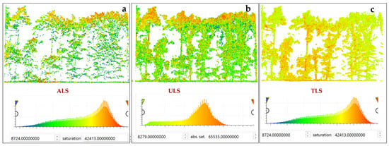
Figure 8. Comparison of LRI distributions across sensing platforms. Panels (a–c) show vertical cross-sections of forest point clouds colored by LRI of ALS, ULS, and TLS, respectively. Corresponding histograms illustrate the LRI distributions for each platform. Differences in intensity magnitude and distribution reflect variations in sensor configuration, range, scan geometry, incidence angle, and platform–target distance, as well as platform-specific radiometric scaling and saturation limits. TLS measurements exhibit higher and broader intensity ranges due to short-range and off-nadir viewing geometry, whereas ALS and ULS LRIs are influenced by flight altitudes (AGL), footprint size, and atmospheric and angular effects. The concurrent open-source TLS, ULS, and ALS datasets were provided by Weiser et al. (2022) [214].

When intensity corrections are applied, LRI serves as the fourth dimension in point clouds and has useful applications in point clouds classification and segmentation [70,174,251]. Currently, most of the commercially available LiDAR sensors are operational in visible, NIR, and shortwave infrared (SWIR) regions of the electromagnetic spectrum (Figure 8). ${ALS}_D$ and ${ALS}_{FW}$ systems onboard aerial platforms, e.g., ALS and ULS, generally operate at 905 nm, 940 nm, and 1064 nm due to the higher reflectance of terrestrial surfaces in NIR, e.g., vegetation (Figure 8a,b and Figure 9). On the other hand, water has high absorption in the NIR region; consequently, a green laser (532 nm) is used for bathymetric applications—specifically, for mapping the floor of shallow coastal waters and lakes [199]. The PCL systems are also operational at 532 nm and 1550 nm [174]. Commercially available LiDAR sensor wavelengths, their career platform, applications, advantages, and limitations are provided in Table 4.

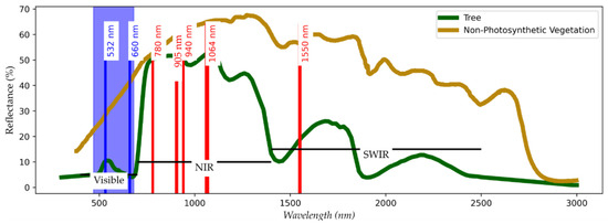
Figure 9. The Advanced Spaceborne Thermal Emission Reflection Radiometer (ASTER) spectral library version 2.0 [278] based on the spectral response of green vegetation (tree) and non-photosynthetic vegetation (NPV). Vertical lines, blue and red, depict the wavelengths at which LiDAR sensors are operational. The blue region marks the wavelength region that has better water penetration for bathymetric LiDAR applications [227].

Table 4. LiDAR sensors operational at different wavelengths onboard carrier platforms with applications, advantages, and limitations in the study of terrestrial ecosystems. Most of the sensor’s specifications are listed in Table 3.

Wavelength (nm)	Platform	Applications	Advantages	Limitations
532	ALS, MLS	Bathymetric mapping, shallow water surveys, coastal zone mapping	It can penetrate water up to several meters (2–30 m).	Less effective in dense vegetation [254,255].
780	ULS, MLS, SLAM	Object recognition, remote sensing, and autonomous systems	High sensitivity in NIR is used in lower-cost systems.	Limited range and accuracy compared to 905 nm and 1064 nm [166].
905	ULS, MLS, TLS, SLAM	General 3D mapping, object detection	Widely used in compact, lower-cost sensors. Good balance between range and accuracy.	Shorter range compared to 1064 nm and 1550 nm [255].
940	ULS, MLS, TLS, SLAM	Object detection, robotics, autonomous vehicles	Good for low-light and nighttime conditions.	Lower range and resolution for large-scale applications [162].
1064	ULS, TLS, ALS, MLS, SLAM	Topography mapping, forest structure analysis, and high-resolution urban scanning	Excellent vegetation and ground penetration. Suitable for longer-range applications.	Cannot penetrate water [279].
1550	ULS, TLS, ALS, MLS, SLAM	Environmental monitoring, vegetation mapping, and urban modeling	High reflectivity from vegetation and terrain.	Reduced water penetration [255].

4.4.5. Laser Health Hazards and Safety Protocols

LiDAR systems primarily operate in the NIR and SWIR regions of the electromagnetic spectrum (Table 4), which are invisible to the human eye, making accidental exposure possible without appropriate safety procedures [182]. Lasers operating at wavelengths ≥ 1500 nm are generally considered eye-safe, whereas many LiDAR systems operate at 1064 nm (Table 4), for which direct eye exposure is hazardous [177]. Single-photon LiDAR (SPL) systems are comparatively less hazardous due to their substantially lower pulse energy and operation at eye-safe wavelengths (e.g., 1550 nm and 532 nm) [280,281]. In contrast, TLS, MLS, SLAM, BLS, and ULS systems operating at lower altitudes require strict eye-safety measures, as they pose greater risks to humans, animals, and birds than ALS and space-borne LiDAR platforms [280,282].

To this end, the above description is an overall understanding of laser systems from their wavelength potential hazard perspective. To the other end, the laser systems are classified (Class 1, 1C, 1M, 2, 2M, 3R, 3B, and 4), and LiDAR products are class-labeled based on their hazard level [283]. Class 1 lasers are considered non-hazardous and pose no known health risks [182]. Class 2 lasers are generally low-risk, with potential harm occurring only if an individual deliberately stares into the beam for extended periods. Lasers classified as Class 1C, 1M, 2M, and 3R may present hazards if not operated correctly; however, the likelihood of injury remains relatively low under normal use. In contrast, Class 3B and Class 4 lasers are highly hazardous, presenting significant health risks, including permanent eye damage or skin burns, if used improperly or without the necessary personal protective equipment and adequate understanding of the associated risks [284]. To use laser sensors, crew members are advised to look for one of the above classification labels printed on the device (see Figure 10).

Figure 10. Laser hazard class labeling on LiDAR sensors allows operators to assess potential hazards and follow class-specific safety protocols before operation. Most LiDAR sensors are equipped with Class 1 lasers to ensure human and environmental safety.

5. Multispectral, Hyperspectral, and Multitemporal LRS

Spectral resolutions of optical satellites are much higher than those of LiDAR sensors. Landsat and Sentinel 1 and 2 satellites are simultaneously operating in RGB, NIR, SWIR, and thermal regions or electromagnetic spectrum, while LiDAR sensors, e.g., ALS, GEDI, and ICESat-2, are operational at a single wavelength [15,16]. Moreover, medium-resolution optical datasets are collected at global scales with a temporal resolution of a few days, e.g., Landsat, Sentinel, and many other commercial satellites [15,134]. VHR optical imagery from satellites, aerial, and ULS are effective in presenting the forest’s physiological response, while the forest’s structural attributes are derived from LiDAR datasets [17,30,226]. LiDAR lacks higher spectral and temporal resolution compared with optical sensors, but is more effective in segmentation and classification when MSL or HSL data is made available [97,142,255,285].

Multi-Temporal, Multispectral, and Hyperspectral Laser Scanning

Repetitive LiDAR surveys over a given area are challenging [211] compared with optical remotely sensed datasets that are geometrically and radiometrically calibrated and harmonized with a fixed-pixel-based analysis [162,251,286]. Ideally, for multitemporal LiDAR data collection, a standard protocol is as follows: LiDAR surveys should be conducted with the same LiDAR sensor with comparable flight and sensor operational parameters, such as scan angles, flight direction, and PRR [94,162,206]. Moreover, surveys should be performed during favorable weather conditions: cloudy and rainy seasons are not ideal due to LiDAR signal degradation, and lower reflectance from wet surfaces [177,286]. In the context of forest ecosystems, forest type (e.g., needle leaf or broad leaf), seasonality (leaf-on or leaf-off), and phenological stages affect the LiDAR backscatter; for instance, laser pulses penetrate through the canopies during the leaf-off season [18,70,94,162]. To offset the seasonality effect on the multitemporal LiDAR data, surveys are performed during the same season of the year. Multitemporal LiDAR data collected following the above state protocol are less complicated for vertical change detection (CD), e.g., Differencing of DEMs (DoD) and Iterative Closest Point (ICP) methods [50,96,233].

However, in practice, available multitemporal LiDAR datasets originate from sensors operating at different wavelengths, with varying operational parameters, and onboard different carrier platforms, e.g., ALS, ULS, and TLS, thus making it challenging to quantify model transferability to other sites [65,119,287]. Even LiDAR sensors with identical flight and sensor parameters, yet different wavelengths, may interact with vegetation differently due to variations in beam divergence (mrad), transmittance, and absorption by terrestrial objects [254]. Thus, a height difference (ICP) between two concurrent points from the same treetop at different wavelengths may be a false positive, as one wavelength could better reflect from leaves (λ = 905 nm) while the other (λ = 1550 nm) is transmitted through leaves and reflected from underlying branches or the tree trunk [255,288]. On the contrary, concurrently operating LiDAR units at different wavelengths capture different geometric structures of plants and trees; therefore, cumulative MSL datasets offer much richer/complete geometric and spectral representation than single-wavelength LiDAR units [173,190]. Currently, dual-wavelength LiDAR sensors are operational at commercial scales and have proven to be more robust than single-wavelength LiDAR systems. Dual-wavelength LiDAR systems offer much deeper insight into the physiological characteristics of vegetation [46,129]. Generally, dual-wavelength systems onboard two laser scanners operating at two different wavelengths: most such configurations have laser scanners operating at 532 nm and 1064 nm concurrently [289]. This is an intelligent approach to collecting MSL datasets using single-wavelength LiDAR units [254,255]. With the development of Hybrid Measurement Unit (HMU), Hybrid Orientation Systems (HOS), and Hybrid Navigation Systems (HNS), compact LiDAR sensors are gaining much attention for commercial applications at unprecedented resolutions, and concurrent use has become more practical [290]. A single LiDAR unit operational at several wavelengths, analogous to an MS camera, has been a technological constraint [285]. Given that the early development in lasing material, e.g., NAGYaG, lacks simultaneous population inversion at different wavelengths (Figure 4). In recent years, MSL and multitemporal LiDAR systems—such as ULS, SLAM, MLS, and TLS—have become increasingly operational, enabling the generation of spectrally enriched and structurally comprehensive datasets that help to address the challenges of fusing LiDAR data with optical imagery [50,166,174].

Recently, significant advances have led to the conception and development of airborne Hyperspectral Imaging LiDAR (HSI-LiDAR) systems [172,252,291]. Supercontinuum laser sources capable of emitting broadband pulses spanning 450–2400 nm have been demonstrated for vegetation and material characterization [252,292]. Several laser technologies have contributed to these developments, including Q-switched fiber lasers [252,293], diode lasers [294], mid-IR fiber lasers [158,295], and newly developed yellow lasers operating between 560 and 600 nm [296], unlike single-wavelength LiDAR systems ${ALS}_D$, ${ALS}_{FW}$, PCL, ICESat-2, and GEDI, which are widely used for large-area mapping. Aside from a few multispectral airborne systems, e.g., the Optech Titan operating at 1550 nm, 1064 nm, and 532 nm [49], HSL operational use is still limited to laboratory measurements, e.g., the spectral response of plants and tree species [297,298]. Furthermore, it is applied in the creation of synthetic datasets through 3D radiative transfer modeling, utilizing the LESS and PROSPECT-4 models [142,148,299], and in basic physical system conceptualization [172]. For the data processing end, new algorithms have been developed for multi-waveform classification of HSL data [51,285,297].

To address the limitations of wide-area MSL/HSL data, hyperspectral systems combine hyperspectral imagery with LiDAR to produce 3D hyperspectral datasets for forestry applications, e.g., to enhance tree species classification [47,55,300]. For data fusion approaches, metrics representative of vegetation composition, productivity, and disturbance are generally acquired from MS/HS imagery, while metrics representative of vertical structures are extracted from classified point clouds, e.g., DSM, CHM, VHM, or LiDAR metrics directly from raw point clouds [32,124]. The LiDAR data fusion approach is generally carried out at local, national, continental, or global scales [74,301]. At local scales, ULS equipped with MSL and HSL imaging sensors operating simultaneously with LiDAR sensor(s) collect concurrent high-resolution spectral and structural datasets [206,223]. The concurrency ensures that radiometric, geometric, and environmental conditions stay the same during surveys [81,302]. Crewed aircraft, e.g., NASA’s G-LiHT, which comprises LiDAR, HS, and thermal sensors operational concurrently, provide an example of collecting data at a larger geographic extent [94]. Secondly, forest ecosystem dynamics investigations are generally carried out at national, continental, and global scales; therefore, aerial platforms, e.g., ULS, provide a concurrent high-resolution ground truth to validate the global products [31,155].

6. Advances in LiDAR Data Processing

6.1. Point Clouds Processing

Data processing performed directly on point clouds (input) to produce a more advanced version of point clouds (output) through automated or semi-automated workflows is referred to as point cloud processing. For example, when point clouds are input into classification/segmentation algorithms, the output point clouds contain unique identity labels, e.g., terrain points (ground) or off-the-terrain (OT) points [303,304]. OT features—including trees, buildings, bridges, as well as electric poles and wires—are man-made or natural objects elevated above the ground, and are further classified/segmented into their respective classes based on their geometrical identity and reflectance properties inferred from Intensity information [18,251] (see Figure 8). The geometric richness of OT objects is subject to LiDAR sensor quality and carrier platforms, e.g., point clouds acquired with TLS and MLS provide geometric richness up to stems, leaves, and branches (Figure 6), while point clouds originating from ALS only present the ground and fuzzy/incomplete OT objects (Figure 6c). Ground and non-ground classification is the most important step towards LiDAR data processing [220]. Point cloud classification/segmentation is useful to develop derivative products, e.g., DEM/DTM, that can be fused and integrated with other remotely sensed datasets, e.g., MS/HS imagery [180,191]. Point cloud classification or segmentation is further classified into two broad categories: parametric algorithms-based approaches and non-parametric ML/DL approaches [305]. Herein, we present one example of each category.

Parametric algorithms are based on simple-to-complex mathematical formulations to capture the characteristics of mathematical representations available in 3D LiDAR datasets [220]. For example, the cloth simulation function (CSF) [306] is used to segregate ground points from OT points—a common ground classification algorithm. In CSF, point clouds (Figure 11a) are first inverted (upside down), and then a cloth is simulated over the inverted point clouds (Figure 11b). Following the cloth simulation, the cloth resolution is defined using cloth particles, e.g., red dots in Figure 11b. The cloth particles move under the influence of gravity. After several iterations, the simulated cloth no longer adjusted its shape under the influence of gravity. Finally, points from the original point cloud that stick with the simulated cloth are classified as ground points [220]. The ground point classification is unsupervised, i.e., no prior information on ground and non-ground point classification or respective labels is required. However, being a parametric method, cloth resolution, terrain slope effect, and cloth rigidity, i.e., how much cloth must bend under the influence of gravity, are the user-defined parameters that need to be adjusted to obtain optimum classification results. Just like CSF, many other ground classification algorithms have been developed in the past, e.g., progressive morphological filter (PMF), and Multiclass Curvature Classification (MCC) are widely used parametric ground classification algorithms [220,306,307]. To extract the meaningful information from point clouds, i.e., features with some geometric fidelity (e.g., stems, branches, and foliage), the unsupervised clustering algorithms have been developed and extensively used. These include Density-Based Spatial Clustering of Applications with Noise (DBSCAN) and its density-robust variant HDBSCAN. Additionally, region-growing algorithms—such as Euclidean, normal-based, and curvature-based methods—and geometric primitive fitting are employed to fit parametric shapes to point subsets. Specific techniques include RANSAC-based cylinder fitting for stems and branches, Hough Transform, and least-squares cylinder or cone fitting. Furthermore, graph-based and connectivity methods, such as minimum spanning tree (MST), spectral clustering, and adjacency-based connected component labeling, are applied in tasks like DBH estimation, stem taper modeling, and branch architecture reconstruction (e.g., Quantitative Structure Modeling (QSM) of trees) [213].

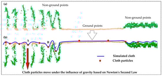
Figure 11. Illustration of the CSF for ground classification. (a) Original LiDAR point cloud showing ground (orange) and non-ground (green) points. (b) Inverted point cloud with a simulated cloth surface (blue line) and discrete cloth particles (red dots) settling under gravity with RI values 3 at A, 2 at B, and 1 at C, respectively, where the cloth conforms to the terrain and separates ground from non-ground points based on local surface geometry. Further reading is available at [220].

The pitfall of parametric algorithms is their user-defined sensitive parameters; these must be tuned for different topographic conditions and/or point clouds’ geometric richness to obtain the desirable segmentation results [220].

Alternatively, ML/DL are non-parametric, yet extensive labeled point clouds that are necessary to train models that can capture the data complexities and topographic representativeness at large expenses [213]. Furthermore, through training and validation, the DL framework needs to be adjusted to train a robust model generalized to unseen data. Among deep learning frameworks, Convolution Neural Networks (CNNs) are widely used for point cloud classification and segmentation [308]. Among CNNs, the architecture is further classified into two groups: CNNs directly operational on point clouds (PointNet, PointNet++, DGCNN, KEConv, PointCNN, Point Transformer, Point-MAE, Point-BERT, and PointNext, etc.) and CNNs that transform 3D point clouds into 2D raster images before classification or segmentation (e.g., RangeNet++, and SalsaNext frameworks) [215,309,310,311]. For raster-based CNN approaches, some information during data transformation from point clouds to raster images is lost [312,313].

The rasterization of 3D point geometries is important given that point clouds are unordered 3D point representations, and therefore, it poses two challenges in the ML/DL data processing context; convolutional operations (CNNs) on unordered point clouds are extremely challenging unless data is subject to some transformation [213]. Secondly, the 3D point observations in time and space produce massive point clouds, making the data processing computationally extensive [220]. Following to pixelation, the point clouds have extensively been transformed into voxelization—a 3D cubical representation of point geometries. This process helps to reduce the structural complexities and massive data size, making them more adoptable for ML/DL applications. These applications include frameworks like VoxelNet, SECOND, PointPillars, MinkowskiNet/Minkowski Engine Family, and sparse convolutional UNets for large-scale 3D segmentation [94,119,310].

6.2. Derivative Products and LiDAR-Based Metrics

DEM, DTM, and CHM, or Vegetation Height Model (VHM), are the most widely used derivative products that originate from classified point cloud data [191,308,314]. DEMs are developed from bare earth points, while DSM, CHM, and VHM are developed from points classified as trees/vegetation [308,314]. The derivative products are gridded surfaces with a fixed pixel size, therefore useful to extract structural metrics, e.g., slope, aspect, soil wetness index (SWI), mean canopy height (MCH), individual tree height, and individual tree crown detection that supports the forest structural and functional attributes (Table 1 and Table 2) [307,315].

The other derivative products are extracted from unclassified/segmented point clouds representative of forest structural complexities, e.g., extracting planar surfaces from point clouds in an unsupervised manner [166]. Feature extraction helps to understand the forest complexities or geometric richness of acquired data. Planar surfaces may indicate manmade structures in urban forests, while cylindrical and elliptical features can represent stems, branches, and leaves [53]. Unlike supervised and unsupervised point cloud classification/segmentation, and raster-based derivative products, e.g., CHM, DEM, and DSM, LiDAR metrics statistically represent the vertical structure of vegetation, providing insights into forest ecosystem complexity and function [76,152]. For example, within a given area of interest (AOI), canopy maximum height, mean height, height standard deviation, percentile of vegetation height, e.g., 25th, 50th, 75th, and 95th, coefficient of variation in vegetation height, Shannon index, Kurtosis of vegetation height, Skewness of vegetation height, variance of vegetation height, etc., are useful LiDAR metrics that can be obtained directly from unclassified/segmented LiDAR datasets originating from ${ALS}_D$, ${ALS}_{FW}$, GEDI, and ICESat-2 [43,129,155,244].

6.3. Open-Source Data Access

We compiled a curated set of freely available open-source LiDAR datasets to support experimental and educational applications, enabling testing, validation, and analysis of point-cloud and waveform data [162,183]. These datasets facilitate the development and benchmarking of new data-processing workflows [315], comparative evaluation of sensor modalities and forest structural metrics [13], and the design of ML/DL pipelines when LiDAR data availability or collection is limited [316].

7. Discussion

7.1. LRS as a Unifying Framework for Vegetation Ecosystems

LRS has evolved from a traditional topographic mapping technique into modern state-of-the-art technology to deeply investigate the vegetation ecosystem’s complexities and spatiotemporal dynamics in 3D space [114]. The present review demonstrated how LRS captures vegetation complexity across domains and scales—from individual plant architecture to landscape-level AGB and fuel structure [9,155,208]—through the integration of geometric, radiometric, and temporal dimensions [94,96,274,317]. The structural, compositional, and functional attributes discussed earlier (Section 2) form the basis for quantifying complex forest ecosystems, cropland, and grassland heterogeneity [31,61,240], while the review of LiDAR sensor modalities $({ALS}_D$, ${ALS}_{FW}$, and PCL), along with carrier platforms (Section 4), illustrates how recent developments have enabled the acquisition of five-dimensional (5D) ecosystem information in space and time. This 5D data integrates geometry (x, y, z), LRI (Figure 8), and multitemporality [61,215,228]. These advances highlight LRS’s key role in producing precise and scalable vegetation ecosystem models [143,318]. MSL and HSL operational modalities, utilizing ${ALS}_D$, ${ALS}_{FW}$, and PCL systems, are emerging by combining spectral and temporal data in one framework, which allows cross-domain analysis, linking forest structural, compositional, productivity, and wildfire dynamics under one methodological umbrella [58,144,173,174,316].

Notwithstanding these advancements, certain technical and conceptual issues persist, which have been thoroughly explained in LiDAR specifications (Section 4.4). These include cross-sensor calibration, waveform decomposition within complex canopies, and the harmonization of LiDAR data with optical and radar observations to achieve comprehensive multi-source integration [182,251,291]. Some key findings are further discussed in the following sub-sections.

7.2. Platform-Dependent Capabilities for Forest Structural Metrics

To understand the platform-dependent capabilities for forest structural metrics detailed in Table 1 and Table 2, we synthesized the relative capability of major LiDAR carrier platforms to retrieve key forest structural and compositional metrics over two decades (Figure 12). The capability matrix highlights that no single platform optimally supports all metrics yet, and that performance is strongly governed by acquisition geometry, spectral wavelengths, lidar modalities, point density, and footprint characteristics. These capabilities may change rapidly in the foreseeable future as MSL and HSL are emerging technological advances in LRS, particularly of aerial and terrestrial platforms, e.g., onboard UAS multispectral and hyperspectral sensors (Figure 12) [49,50,126,174,316].

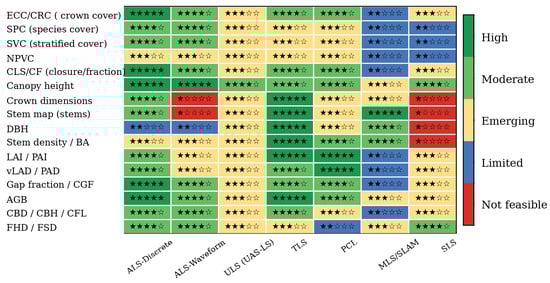
Figure 12. The matrices (Table 1 and Table 2) summarize the relative capability of major LiDAR platforms—ALS, ULS, TLS, PCL, MLS/SLAM, and SLS—to derive key forest structural, canopy, and fuel-related metrics. Star symbols (★–★★★★★) indicate qualitative capability levels, ranging from very limited existing feasibility (★) to high capability, and methodological maturity (★★★★★) as reported in the literature (1999–2025). Background color-coding classifies each platform–metric combination as High (dark green), Moderate (green), Emerging (yellow), Limited (blue), or Not feasible (red). The assessment reflects consensus from peer-reviewed studies and emphasizes complementary strengths and limitations across platforms rather than absolute performance ranking. Derivatives or closely related metrics (Table 1 and Table 2) are not shown explicitly, as they are largely computed from the primary metrics listed above.

Among the existing platforms, ${ALS}_D$ and ${ALS}_{FW}$ consistently play a decisive role in forest ecosystem studies at both regional and national scales, demonstrating strong performance across most metrics listed in Table 1 and Table 2. Figure 12 indicates that these metrics benefit from mature processing pipelines and extensive validation across forest biomes spanning over two decades of ALS surveys [49,61,177]. ${ALS}_D$ have been operational at moderate-to-higher pulse densities, which are insensitive to forest metrics, e.g., tree height, shrub height, and BA [262]. In contrast, stem-level attributes such as DBH, stem density, and crown dimensions exhibit limited feasibility when derived solely from ALS, reflecting well-known occlusion effects under dense canopy conditions (Figure 6c) [94,173].${ ALS}_{FW}$ capture the full backscattered signal and thus richer forest geometry, but their practical use has been constrained in the past due to the complexities of waveform data processing, although more advanced algorithms and DL frameworks are now emerging [51,189,190,194].

Counterpart, TLS demonstrates the strongest capability for fine-scale structural attributes, including DBH [146], stem density [58], CBD [122], ECC [212], CBH [122], fuel strata gap (FSG) [113], assessment of foliage distribution and dynamics owing to its near-isotropic sampling geometry and much higher spatial, spectral and temporal trajectories [97,146,319]—see Figure 6a. In contrast, stem-level metrics exhibit a pronounced temporal transition. Early ALS-based attempts to retrieve DBH or stem density show limited adoption through allometric relationships and imputation modeling, whereas TLS-based approaches display a sharp increase after approximately 2010, coinciding with advances in point-cloud segmentation, QSM, and automated and standardized processing workflows. However, its limited spatial extent constrains direct upscaling (Figure 6d), reinforcing its role as a calibration and validation reference rather than a stand-alone landscape mapping solution [58,319]. In recent times, integration with MLS/SLAM and a global network of TLS plots could extend its application over larger aerial extents of complex forest ecosystems [68,100,202].

To bridge the gap between ALS and TLS, ULS occupies an intermediate position, showing growing capability for both canopy-scale and selected stem-related metrics, particularly in open or moderately dense vegetation (Figure 6b–e); therefore, it is an emerging LiDAR modality (Figure 12) with multiple payload capabilities [206,228,320]. More recently, ULS platforms show accelerating adoption for both canopy- and stem-related metrics, reflecting rapid sensor miniaturization and improved positioning accuracy. MLS/SLAM systems exhibit the most recent adoption peaks, with high saturation limited primarily to stem mapping and plot-scale inventories. MLS/SLAM systems exhibit high capability for stem mapping and corridor-scale inventories but remain limited for canopy-integrated metrics that require full vertical coverage. One particular reason is that the payload size/weight and navigational challenges in complex forest landscapes limit their operational capacity [122,156].

SLS, including GEDI and ICESat-2, provide unparalleled spatiotemporal coverage and demonstrate high capability for vertically integrated area-based metrics (≈25 m) such as canopy height and AGB, while remaining limited as stand-alone technology, yet with the possibility of data fusion and imputation modeling to upscale the mapping resolution to access the temporal trajectories, e.g., forest disturbance and forest age [11,25,31,105,195]. SLS adoption shows punctuated increases associated with mission deployments, emphasizing its role in global monitoring rather than detailed structural reconstruction.

7.3. Across-Platform Differences

The complementary insights provided by Figure 12 underscore the growing importance of multiplatform concurrent LiDAR datasets acquisition (Figure 5). ALS and SLS systems provide spatial continuity and long-term monitoring capability, while TLS and ULS supply structural details necessary for model calibration, AGB modeling, and fuel characterization [58,146]. This hierarchical integration is increasingly critical for ecosystem modeling, particularly where plot-scale measurements must be extrapolated across heterogeneous landscapes [11,214]. Figure 6 further illustrates these geometric differences by contrasting nadir-view ALS and ULS point clouds with side-view TLS observations, highlighting how acquisition perspective fundamentally shapes metric observability [214]. Such differences reinforce the need for scale-aware processing strategies and caution against indiscriminate metric transfer across platforms [45,59,126].

The data-processing and fusion methodologies summarized in Section 6 exemplify how classical geometric algorithms are increasingly augmented by AI and DL frameworks to automate canopy segmentation, feature extraction, and ecosystem classification [215,316,321,322]. These developments mark a shift from descriptive 3D mapping to predictive modeling of ecological processes. However, the performance of AI-driven methods remains constrained by limited reference data, inconsistent acquisition parameters, and a lack of open, standardized benchmarks across biomes, though this trend is shifting under more and more open-source data distribution polices (Table 5) [13]. Future research should therefore focus on unifying calibration protocols, developing transferable models, and fostering open-access LiDAR repositories that facilitate algorithm reproducibility and interoperability among sensor modalities [323].

Table 5. Open-access LiDAR data sources spanning multiple platforms and data products for forest structure analysis and algorithm development.

Organization/Source	Platform	Format	Region
OpenTopography 1 [324]	Multiplatform	Point clouds and derivative products, e.g., DEM, CHM, and DSM	Global
Global TLS 2 [202]	TLS	Point clouds	Global
National Science Foundation (NSF) NeonScience 3 [127]	Multiplatform	Point clouds, waveform, multitemporal, and derivative products, e.g., DEM, CHM, and DSM	Selected eco-regions in the United States
PANGAEA 4 [325]	Multiplatform	Point clouds, waveform, multitemporal, multispectral, and derivative products, e.g., DEM, CHM, and DSM	Global

¹: https://opentopography.org/ (accessed on 18 December 2025); ²: https://www.global-tls.net/ (accessed on 18 December 2025); ³: https://www.neonscience.org/data-collection/lidar (accessed on 18 December 2025); ⁴: https://www.pangaea.de/ (accessed on 18 December 2025). Note: This table is not intended to provide an extensive list of all open-access LiDAR datasets. Instead, it highlights representative and widely used data sources that illustrate the diversity of sensors, platforms, and data types currently available. Access to some datasets may require institutional credentials, user registration, or a direct request to data authors. However, the above-mentioned sources ensure the waveform, point clouds, MSL datasets originating from TLS, MLS, ULS, SLAM, and photogrammetry.

Table 5. Open-access LiDAR data sources spanning multiple platforms and data products for forest structure analysis and algorithm development.

Organization/Source	Platform	Format	Region
OpenTopography 1 [324]	Multiplatform	Point clouds and derivative products, e.g., DEM, CHM, and DSM	Global
Global TLS 2 [202]	TLS	Point clouds	Global
National Science Foundation (NSF) NeonScience 3 [127]	Multiplatform	Point clouds, waveform, multitemporal, and derivative products, e.g., DEM, CHM, and DSM	Selected eco-regions in the United States
PANGAEA 4 [325]	Multiplatform	Point clouds, waveform, multitemporal, multispectral, and derivative products, e.g., DEM, CHM, and DSM	Global

¹: https://opentopography.org/ (accessed on 18 December 2025); ²: https://www.global-tls.net/ (accessed on 18 December 2025); ³: https://www.neonscience.org/data-collection/lidar (accessed on 18 December 2025); ⁴: https://www.pangaea.de/ (accessed on 18 December 2025). Note: This table is not intended to provide an extensive list of all open-access LiDAR datasets. Instead, it highlights representative and widely used data sources that illustrate the diversity of sensors, platforms, and data types currently available. Access to some datasets may require institutional credentials, user registration, or a direct request to data authors. However, the above-mentioned sources ensure the waveform, point clouds, MSL datasets originating from TLS, MLS, ULS, SLAM, and photogrammetry.

To consolidate the present review and extend the baseline of knowledge on LRS, Table 6 compiles a carefully selected list of recent reviews and research papers that collectively deepen one or more aspects discussed above. These references span topics such as LiDAR radiometric calibration [219], MSL and HSL applications [119], waveform decomposition [169], single-photon technology [288], and AI-based point-cloud classification [287]. Others address the integration of LiDAR with complementary sensors, high-throughput data processing (Laserfarm [290]), and software frameworks like lidR [291] that have become indispensable in forestry analytics. Together, these works bridge theoretical understanding and practical implementation, linking sensor physics, computational techniques, and ecological interpretation [97,252,326]. We also listed some open-source data sources for users with limited availability of multi-sensor LiDAR point clouds to gain hands-on experience in data processing and analysis using open-source software applications for research and educational purposes (Table 5).

By unifying insights across these dimensions, the present discussion underscores that future progress in vegetation-focused LiDAR research will depend on three intertwined pathways: (1) the physical enhancement of sensors toward MSL, HSL, and photon-sensitive modalities [65,78]; (2) the algorithmic evolution toward AI- and physics-based modeling for feature extraction [276,327]; and (3) the establishment of global, standardized LiDAR data infrastructures for consistent, long-term monitoring of terrestrial ecosystems [9,31,68]. In essence, LiDAR is no longer limited to representing topography and forest heights; it has become a quantitative language for describing ecosystem composition, function, ecology, and disturbance status [73,97,152].

Table 6. Selected review and research articles further the in-depth information on forest structural complexity from the LRS of a vegetation perspective.

Title	Supporting Information	Year	Type
A Review of LIDAR Radiometric Processing: From Ad Hoc Intensity Correction to Rigorous Radiometric Calibration [251].	LRI is important information along with the 3D structural complexity of forest ecosystems. However, LRI radiometric and intensity correction methods are important to understand.	2015	Review
Advancements in high-resolution land surface satellite products: A comprehensive review of inversion algorithms, products, and challenges [328].	Understanding satellite data products helps in data fusion with different LiDAR datasets for forest ecosystem mapping and modeling.	2024	Review
Beyond 3D: The new spectrum of lidar applications for the earth and ecological sciences [275].	A very important contribution that helps to understand the LiDAR intensity (LRI) application in terrestrial ecosystem investigations.	2016	Review
Deep Learning for LiDAR Point Cloud Classification in Remote Sensing [329].	Understanding DL approaches for point cloud classification and segmentation.	2022	Review
Decomposition of full-waveform LiDAR data utilizing an adaptive B-spline-based model and particle swarm optimization [185].	A sound mathematical background on different LiDAR waveform decomposition methods was experimented with GEDI waveform data.	2024	Research
Evaluating the capacity of single photon lidar for terrain characterization under a range of forest conditions [330].	Understanding the capabilities of SPL technology is an important milestone toward next-generation LiDAR applications in forest ecosystem studies.	2021	Research
Forest and woodland stand structural complexity: Its definition and measurement [39].	Understanding attributes defining forest structural complexity is important from the LRS and forest management perspective.	2005	Review
Integrated trajectory estimation for 3D kinematic mapping with GNSS, INS, and imaging sensors: A framework and review [331].	Integrating laser scanners with pivotal sister technologies, e.g., GNSS and INS/IMU, is an important technological frontier that needs a mathematical background. This review provides an in-depth insight into this subject.	2023	Review
Laserfarm: A high-throughput workflow for generating geospatial data products of ecosystem structure from airborne laser scanning point clouds [332].	Python-based package for extracting forest ecosystem-related LiDAR metrics from point clouds. Also, provide the download links of European open-access LiDAR data.	2022	Research
Lidar sampling for large-area forest characterization: A review [26].	Sampling forest characterization in wide-area capacity	2012	Review
lidR: An R package for analysis of Airborne Laser Scanning (ALS) data [333].	Several ground point classifications, e.g., CSF, MCC, PMF, and derivative products, e.g., CHMs, DEM, Tree detection, crown segmentation, and many more algorithms have been implemented in the R programming environment.	2020	Research
Peering through the thicket: Effects of UAV LiDAR scanner settings and flight planning on canopy volume discovery [263].	ULS survey planning and sensor parameters optimization over dense forest landscapes. Explains different types of occlusions in relation to different flying altitudes, scanning angles, and PRF.	2020	Research
Review of ground and aerial methods for vegetation cover fraction (fCover) and related quantities estimation: definitions, advances, challenges, and future perspectives [143].	Different vegetation cover fractions for cropland, grassland, and forests are exemplified in the context of different remote sensing carrier platforms and sensors (see Table 1).	2023	Review
Towards a comprehensive and consistent global aquatic land cover characterization framework addressing multiple user needs [334].	Global Aquatic Land Cover datasets (33 data products) are useful for integrating with LiDAR datasets for forest ecosystem dynamics investigations.	2020	Review
Wildfire response of forest species from multispectral LiDAR data. A deep learning approach with synthetic data [316].	A useful contribution to understanding the forest response to multispectral LiDAR datasets in the wildfire context.	2024	Research
Multispectral Light Detection and Ranging Technology and Applications: A Review [50].	A concise review of multispectral LiDAR in ecology and forestry, highlighting current uses and future directions for acquiring multispectral and multitemporal LiDAR data.	2024	Review

Table 6. Selected review and research articles further the in-depth information on forest structural complexity from the LRS of a vegetation perspective.

Title	Supporting Information	Year	Type
A Review of LIDAR Radiometric Processing: From Ad Hoc Intensity Correction to Rigorous Radiometric Calibration [251].	LRI is important information along with the 3D structural complexity of forest ecosystems. However, LRI radiometric and intensity correction methods are important to understand.	2015	Review
Advancements in high-resolution land surface satellite products: A comprehensive review of inversion algorithms, products, and challenges [328].	Understanding satellite data products helps in data fusion with different LiDAR datasets for forest ecosystem mapping and modeling.	2024	Review
Beyond 3D: The new spectrum of lidar applications for the earth and ecological sciences [275].	A very important contribution that helps to understand the LiDAR intensity (LRI) application in terrestrial ecosystem investigations.	2016	Review
Deep Learning for LiDAR Point Cloud Classification in Remote Sensing [329].	Understanding DL approaches for point cloud classification and segmentation.	2022	Review
Decomposition of full-waveform LiDAR data utilizing an adaptive B-spline-based model and particle swarm optimization [185].	A sound mathematical background on different LiDAR waveform decomposition methods was experimented with GEDI waveform data.	2024	Research
Evaluating the capacity of single photon lidar for terrain characterization under a range of forest conditions [330].	Understanding the capabilities of SPL technology is an important milestone toward next-generation LiDAR applications in forest ecosystem studies.	2021	Research
Forest and woodland stand structural complexity: Its definition and measurement [39].	Understanding attributes defining forest structural complexity is important from the LRS and forest management perspective.	2005	Review
Integrated trajectory estimation for 3D kinematic mapping with GNSS, INS, and imaging sensors: A framework and review [331].	Integrating laser scanners with pivotal sister technologies, e.g., GNSS and INS/IMU, is an important technological frontier that needs a mathematical background. This review provides an in-depth insight into this subject.	2023	Review
Laserfarm: A high-throughput workflow for generating geospatial data products of ecosystem structure from airborne laser scanning point clouds [332].	Python-based package for extracting forest ecosystem-related LiDAR metrics from point clouds. Also, provide the download links of European open-access LiDAR data.	2022	Research
Lidar sampling for large-area forest characterization: A review [26].	Sampling forest characterization in wide-area capacity	2012	Review
lidR: An R package for analysis of Airborne Laser Scanning (ALS) data [333].	Several ground point classifications, e.g., CSF, MCC, PMF, and derivative products, e.g., CHMs, DEM, Tree detection, crown segmentation, and many more algorithms have been implemented in the R programming environment.	2020	Research
Peering through the thicket: Effects of UAV LiDAR scanner settings and flight planning on canopy volume discovery [263].	ULS survey planning and sensor parameters optimization over dense forest landscapes. Explains different types of occlusions in relation to different flying altitudes, scanning angles, and PRF.	2020	Research
Review of ground and aerial methods for vegetation cover fraction (fCover) and related quantities estimation: definitions, advances, challenges, and future perspectives [143].	Different vegetation cover fractions for cropland, grassland, and forests are exemplified in the context of different remote sensing carrier platforms and sensors (see Table 1).	2023	Review
Towards a comprehensive and consistent global aquatic land cover characterization framework addressing multiple user needs [334].	Global Aquatic Land Cover datasets (33 data products) are useful for integrating with LiDAR datasets for forest ecosystem dynamics investigations.	2020	Review
Wildfire response of forest species from multispectral LiDAR data. A deep learning approach with synthetic data [316].	A useful contribution to understanding the forest response to multispectral LiDAR datasets in the wildfire context.	2024	Research
Multispectral Light Detection and Ranging Technology and Applications: A Review [50].	A concise review of multispectral LiDAR in ecology and forestry, highlighting current uses and future directions for acquiring multispectral and multitemporal LiDAR data.	2024	Review

8. Conclusions

Laser remote sensing in precision forestry has advanced to a level of development at which its value extends beyond 3D mapping toward integrated ecological measurement and prediction. What began as a topographic ranging technology has progressively evolved into a multi-modal observational framework capable of capturing vegetation structure, composition, and dynamics across spatial and temporal scales. The synthesis presented in this review illustrates how linear-mode, waveform, and photon-counting LiDAR systems—deployed from terrestrial, airborne, and space-borne platforms—now jointly support vegetation monitoring across forests, croplands, and grasslands. At present, the combined use of structural metrics, radiometric information, and multitemporal observations enables unprecedented insight into ecosystem complexity in 3D space, while also exposing persistent limitations related to cross-sensor calibration, data harmonization, and large-scale interoperability.

Within this landscape, the present comprehensive review article plays a critical role by integrating dispersed findings, evaluating methodological frameworks, and identifying the potential applications of forest metrics in interdisciplinary studies. By systematically organizing evidence across platforms, ecosystems, and application domains, such syntheses provide a common reference frame that guides sensor development, sensor selection based on their strengths and weaknesses, field protocol design, model selection, and data-fusion strategies, thereby amplifying the impact of individual case studies. Looking ahead, the most significant advances in vegetation laser remote sensing are expected to arise from the integration of multispectral and hyperspectral LiDAR, dense time-series acquisitions, and artificial-intelligence-driven analytics within standardized and open frameworks. These developments—underpinned by ongoing critical reviews—will strengthen structural–spectral coupling, reduce uncertainties in AGB, fuel, and disturbance estimates, and support scalable, near-real-time ecosystem monitoring. In this context, LiDAR is positioned not only as a core observational technology but as an enabling infrastructure for long-term vegetation assessment, ecosystem management, and climate-relevant decision-making.

References

- Feng, K.; Ma, S.; Xi, H.; Liang, L.; Liu, W.; Tsunekawa, A. Small-sample-data augmentation and transfer strategies for forest cover change monitoring. Ecol. Indic. 2025, 178, 113870. [Google Scholar] [CrossRef]
- Afuye, G.A.; Nduku, L.; Kalumba, A.M.; Santos, C.A.G.; Orimoloye, I.R.; Ojeh, V.N.; Thamaga, K.H.; Sibandze, P. Global trend assessment of land use and land cover changes: A systematic approach to future research development and planning. J. King Saud Univ. Sci. 2024, 36, 103262. [Google Scholar] [CrossRef]
- Peters, F.; Lippe, M.; Eguiguren, P.; Günter, S. Forest ecosystem services at landscape level—Why forest transition matters? For. Ecol. Manag. 2023, 534, 120782. [Google Scholar] [CrossRef]
- Piao, S.; Zhang, X.; Chen, A.; Liu, Q.; Lian, X.; Wang, X.; Peng, S.; Wu, X. The impacts of climate extremes on the terrestrial carbon cycle: A review. Sci. China Earth Sci. 2019, 62, 1551–1563. [Google Scholar] [CrossRef]
- Smith-Ramírez, C.; Grez, A.; Galleguillos, M.; Cerda, C.; Ocampo-Melgar, A.; Miranda, M.D.; Muñoz, A.A.; Rendón-Funes, A.; Díaz, I.; Cifuentes, C.; et al. Ecosystem services of Chilean sclerophyllous forests and shrublands on the verge of collapse: A review. J. Arid Environ. 2023, 211, 104927. [Google Scholar] [CrossRef]
- Gholizadeh, H.; Friedman, M.S.; McMillan, N.A.; Hammond, W.M.; Hassani, K.; Sams, A.V.; Charles, M.D.; Garrett, D.R.; Joshi, O.; Hamilton, R.G.; et al. Mapping invasive alien species in grassland ecosystems using airborne imaging spectroscopy and remotely observable vegetation functional traits. Remote Sens. Environ. 2022, 271, 112887. [Google Scholar] [CrossRef]
- Hisano, M.; Searle, E.B.; Chen, H.Y.H. Biodiversity as a solution to mitigate climate change impacts on the functioning of forest ecosystems: Biodiversity to mitigate climate change impacts. Biol. Rev. 2018, 93, 439–456. [Google Scholar] [CrossRef]
- White, J.C.; Hermosilla, T.; Wulder, M.A.; Coops, N.C. Mapping, validating, and interpreting spatio-temporal trends in post-disturbance forest recovery. Remote Sens. Environ. 2022, 271, 112904. [Google Scholar] [CrossRef]
- Shaw, D.C.; Beedlow, P.A.; Henry Lee, E.; Woodruff, D.R.; Meigs, G.W.; Calkins, S.J.; Reilly, M.J.; Merschel, A.G.; Cline, S.P.; Comeleo, R.L. The complexity of biological disturbance agents, fuels heterogeneity, and fire in coniferous forests of the western United States. For. Ecol. Manag. 2022, 525, 120572. [Google Scholar] [CrossRef]
- Zhang, J.; Wang, J.; Liu, G. Vertical Structure Classification of a Forest Sample Plot Based on Point Cloud Data. J. Indian Soc. Remote Sens. 2020, 48, 1215–1222. [Google Scholar] [CrossRef]
- Guerra-Hernández, J.; Pereira, J.M.C.; Stovall, A.; Pascual, A. Impact of fire severity on forest structure and biomass stocks using NASA GEDI data. Insights from the 2020 and 2021 wildfire season in Spain and Portugal. Sci. Remote Sens. 2024, 9, 100134. [Google Scholar] [CrossRef]
- Zheng, Z.; Zeng, Y.; Schneider, F.D.; Zhao, Y.; Zhao, D.; Schmid, B.; Schaepman, M.E.; Morsdorf, F. Mapping functional diversity using individual tree-based morphological and physiological traits in a subtropical forest. Remote Sens. Environ. 2021, 252, 112170. [Google Scholar] [CrossRef]
- Ehbrecht, M.; Seidel, D.; Annighöfer, P.; Kreft, H.; Köhler, M.; Zemp, D.C.; Puettmann, K.; Nilus, R.; Babweteera, F.; Willim, K.; et al. Global patterns and climatic controls of forest structural complexity. Nat. Commun. 2021, 12, 519. [Google Scholar] [CrossRef] [PubMed]
- Heilmeier, H. Functional traits explaining plant responses to past and future climate changes. Flora 2019, 254, 1–11. [Google Scholar] [CrossRef]
- Travers-Smith, H.; Coops, N.C.; Mulverhill, C.; Wulder, M.A.; Ignace, D.; Lantz, T.C. Mapping vegetation height and identifying the northern forest limit across Canada using ICESat-2, Landsat time series and topographic data. Remote Sens. Environ. 2024, 305, 114097. [Google Scholar] [CrossRef]
- Claverie, M.; Ju, J.; Masek, J.G.; Dungan, J.L.; Vermote, E.F.; Roger, J.-C.; Skakun, S.V.; Justice, C. The Harmonized Landsat and Sentinel-2 surface reflectance data set. Remote Sens. Environ. 2018, 219, 145–161. [Google Scholar] [CrossRef]
- Lechner, A.M.; Foody, G.M.; Boyd, D.S. Applications in Remote Sensing to Forest Ecology and Management. One Earth 2020, 2, 405–412. [Google Scholar] [CrossRef]
- Alexander, C.; Bøcher, P.K.; Arge, L.; Svenning, J.-C. Regional-scale mapping of tree cover, height and main phenological tree types using airborne laser scanning data. Remote Sens. Environ. 2014, 147, 156–172. [Google Scholar] [CrossRef]
- DiMiceli, C.; Townshend, J.; Carroll, M.; Sohlberg, R. Evolution of the representation of global vegetation by vegetation continuous fields. Remote Sens. Environ. 2021, 254, 112271. [Google Scholar] [CrossRef]
- Potapov, P.; Li, X.; Hernandez-Serna, A.; Tyukavina, A.; Hansen, M.C.; Kommareddy, A.; Pickens, A.; Turubanova, S.; Tang, H.; Silva, C.E.; et al. Mapping global forest canopy height through integration of GEDI and Landsat data. Remote Sens. Environ. 2021, 253, 112165. [Google Scholar] [CrossRef]
- Shendryk, Y. Fusing GEDI with earth observation data for large area aboveground biomass mapping. Int. J. Appl. Earth Obs. Geoinf. 2022, 115, 103108. [Google Scholar] [CrossRef]
- Montesano, P.M.; Neigh, C.; Sun, G.; Duncanson, L.; Hoek, J.V.D.; Jon Ranson, K. The use of sun elevation angle for stereogrammetric boreal forest height in open canopies. Remote Sens. Environ. 2017, 196, 76–88. [Google Scholar] [CrossRef] [PubMed]
- Tuominen, S.; Balazs, A.; Saari, H.; Pölönen, I.; Sarkeala, J.; Viitala, R. Unmanned aerial system imagery and photogrammetric canopy height data in area-based estimation of forest variables. Silva Fenn. 2015, 49, 1348. [Google Scholar] [CrossRef]
- Kimura, T.; Imai, T.; Sakaizawa, D.; Murooka, J.; Mitsuhashi, R. The overview and status of vegetation Lidar mission, MOLI. In Proceedings of the 2017 IEEE International Geoscience and Remote Sensing Symposium (IGARSS), Fort Worth, TX, USA, 23–28 July 2017; pp. 4228–4230. [Google Scholar]
- Luo, H.; Ou, G.; Yue, C.; Zhu, B.; Wu, Y.; Zhang, X.; Lu, C.; Tang, J. A framework for montane forest canopy height estimation via integrating deep learning and multi-source remote sensing data. Int. J. Appl. Earth Obs. Geoinf. 2025, 138, 104474. [Google Scholar] [CrossRef]
- Wulder, M.A.; White, J.C.; Nelson, R.F.; Næsset, E.; Ørka, H.O.; Coops, N.C.; Hilker, T.; Bater, C.W.; Gobakken, T. Lidar sampling for large-area forest characterization: A review. Remote Sens. Environ. 2012, 121, 196–209. [Google Scholar] [CrossRef]
- Jin, P.; Xu, M.; Yang, Q.; Zhang, J. The influence of stand composition and season on canopy structure and understory light environment in different subtropical montane Pinus massoniana forests. PeerJ 2024, 12, e17067. [Google Scholar] [CrossRef]
- Horning, N. Remote Sensing. In Encyclopedia of Ecology, 2nd ed.; Fath, B., Ed.; Elsevier: Oxford, UK, 2019; pp. 404–413. [Google Scholar]
- Le Louëdec, J.; Cielniak, G. 3D shape sensing and deep learning-based segmentation of strawberries. Comput. Electron. Agric. 2021, 190, 106374. [Google Scholar] [CrossRef]
- Vyvlečka, P.; Pechanec, V. Optical Remote Sensing in Provisioning of Ecosystem-Functions Analysis-Review. Sensors 2023, 23, 4937. [Google Scholar] [CrossRef]
- de Conto, T.; Armston, J.; Dubayah, R. Characterizing the structural complexity of the Earth’s forests with spaceborne lidar. Nat. Commun. 2024, 15, 8116. [Google Scholar] [CrossRef]
- Crookston, N.L.; Dixon, G.E. The forest vegetation simulator: A review of its structure, content, and applications. Comput. Electron. Agric. 2005, 49, 60–80. [Google Scholar] [CrossRef]
- Swann, D.E.B.; Fried, J.S.; Gray, A.N. Evaluating Forest Vegetation Simulator (FVS) calibration options for predicting biomass accumulation across diverse Oregon landscapes. For. Ecol. Manag. 2025, 594, 122937. [Google Scholar] [CrossRef]
- Bagdon, B.A.; Nguyen, T.H.; Vorster, A.; Paustian, K.; Field, J.L. A model evaluation framework applied to the Forest Vegetation Simulator (FVS) in Colorado and Wyoming lodgepole pine forests. For. Ecol. Manag. 2021, 480, 118619. [Google Scholar] [CrossRef]
- Woods, M.; Pitt, D.; Penner, M.; Lim, K.; Nesbitt, D.; Etheridge, D.; Treitz, P. Operational implementation of a LiDAR inventory in Boreal Ontario. For. Chron. 2011, 87, 512–528. [Google Scholar] [CrossRef]
- Wulder, M.A.; Bater, C.W.; Coops, N.C.; Hilker, T.; White, J.C. The role of LiDAR in sustainable forest management. For. Chron. 2008, 84, 807–826. [Google Scholar] [CrossRef]
- Barrett, F.; McRoberts, R.E.; Tomppo, E.; Cienciala, E.; Waser, L.T. A questionnaire-based review of the operational use of remotely sensed data by national forest inventories. Remote Sens. Environ. 2016, 174, 279–289. [Google Scholar] [CrossRef]
- Legg, C.J.; Nagy, L. Why most conservation monitoring is, but need not be, a waste of time. J. Environ. Manag. 2006, 78, 194–199. [Google Scholar] [CrossRef]
- McElhinny, C.; Gibbons, P.; Brack, C.; Bauhus, J. Forest and woodland stand structural complexity: Its definition and measurement. For. Ecol. Manag. 2005, 218, 1–24. [Google Scholar] [CrossRef]
- Aragoneses, E.; García, M.; Tang, H.; Chuvieco, E. A multi-sensor approach allows confident mapping of forest canopy fuel load and canopy bulk density to assess wildfire risk at the European scale. Remote Sens. Environ. 2025, 318, 114578. [Google Scholar] [CrossRef]
- Masek, J.G.; Hayes, D.J.; Joseph Hughes, M.; Healey, S.P.; Turner, D.P. The role of remote sensing in process-scaling studies of managed forest ecosystems. Carbon Water Nutr. Cycl. Manag. For. 2015, 355, 109–123. [Google Scholar] [CrossRef]
- Kelly, M.; Tommaso, S.D. Mapping forests with Lidar provides flexible, accurate data with many uses. Calif. Agric. 2015, 69, 14–20. [Google Scholar] [CrossRef]
- Chan, E.P.Y.; Fung, T.; Wong, F.K.K. Estimating above-ground biomass of subtropical forest using airborne LiDAR in Hong Kong. Sci. Rep. 2021, 11, 1751. [Google Scholar] [CrossRef] [PubMed]
- Hudak, A.T.; Evans, J.S.; Stuart Smith, A.M. LiDAR Utility for Natural Resource Managers. Remote Sens. 2009, 1, 934–951. [Google Scholar] [CrossRef]
- Beland, M.; Parker, G.; Sparrow, B.; Harding, D.; Chasmer, L.; Phinn, S.; Antonarakis, A.; Strahler, A. On promoting the use of lidar systems in forest ecosystem research. For. Ecol. Manag. 2019, 450, 117484. [Google Scholar] [CrossRef]
- Wang, C.-K.; Tseng, Y.-H.; Chu, H.-J. Airborne Dual-Wavelength LiDAR Data for Classifying Land Cover. Remote Sens. 2014, 6, 700–715. [Google Scholar] [CrossRef]
- Alonzo, M.; Bookhagen, B.; Roberts, D.A. Urban tree species mapping using hyperspectral and lidar data fusion. Remote Sens. Environ. 2014, 148, 70–83. [Google Scholar] [CrossRef]
- Lefsky, M.A.; Cohen, W.B.; Acker, S.A.; Parker, G.G.; Spies, T.A.; Harding, D. Lidar Remote Sensing of the Canopy Structure and Biophysical Properties of Douglas-Fir Western Hemlock Forests. Remote Sens. Environ. 1999, 70, 339–361. [Google Scholar] [CrossRef]
- Lindberg, E.; Holmgren, J.; Olsson, H. Classification of tree species classes in a hemi-boreal forest from multispectral airborne laser scanning data using a mini raster cell method. Int. J. Appl. Earth Obs. Geoinf. 2021, 100, 102334. [Google Scholar] [CrossRef]
- Takhtkeshha, N.; Mandlburger, G.; Remondino, F.; Hyyppä, J. Multispectral Light Detection and Ranging Technology and Applications: A Review. Sensors 2024, 24, 1669. [Google Scholar] [CrossRef]
- Li, X.; Shao, H.; Lu, Y.; Chen, Y.; Sun, L.; Dai, H.; Hong, T.; Zhang, X.; Zhang, H. An enhance ranging algorithm based on multi-waveform classification with hyperspectral LiDAR. Measurement 2025, 253, 117489. [Google Scholar] [CrossRef]
- Tang, H.; Song, X.-P.; Zhao, F.A.; Strahler, A.H.; Schaaf, C.L.; Goetz, S.; Huang, C.; Hansen, M.C.; Dubayah, R. Definition and measurement of tree cover: A comparative analysis of field-, lidar- and landsat-based tree cover estimations in the Sierra national forests, USA. Agric. For. Meteorol. 2019, 268, 258–268. [Google Scholar] [CrossRef]
- César de Lima Araújo, H.; Silva Martins, F.; Tucunduva Philippi Cortese, T.; Locosselli, G.M. Artificial intelligence in urban forestry—A systematic review. Urban For. Urban Green. 2021, 66, 127410. [Google Scholar] [CrossRef]
- Abdollahi, A.; Yebra, M. Forest fuel type classification: Review of remote sensing techniques, constraints and future trends. J. Environ. Manag. 2023, 342, 118315. [Google Scholar] [CrossRef] [PubMed]
- Kazanskiy, N.L.; Doskolovich, L.L.; Golovastikov, N.V.; Khonina, S.N. The power of fusion: LiDAR meets hyperspectral imaging in a new era of exploration. Opt. Laser Technol. 2025, 192, 114080. [Google Scholar] [CrossRef]
- Proudman, A.; Ramezani, M.; Digumarti, S.T.; Chebrolu, N.; Fallon, M. Towards real-time forest inventory using handheld LiDAR. Robot. Auton. Syst. 2022, 157, 104240. [Google Scholar] [CrossRef]
- Tatsumi, S.; Yamaguchi, K.; Furuya, N. ForestScanner: A mobile application for measuring and mapping trees with LiDAR-equipped iPhone and iPad. Methods Ecol. Evol. 2023, 14, 1603–1609. [Google Scholar] [CrossRef]
- Liang, X.; Kankare, V.; Hyyppä, J.; Wang, Y.; Kukko, A.; Haggrén, H.; Yu, X.; Kaartinen, H.; Jaakkola, A.; Guan, F.; et al. Terrestrial laser scanning in forest inventories. ISPRS J. Photogramm. Remote Sens. 2016, 115, 63–77. [Google Scholar] [CrossRef]
- Bruggisser, M.; Hollaus, M.; Otepka, J.; Pfeifer, N. Influence of ULS acquisition characteristics on tree stem parameter estimation. ISPRS J. Photogramm. Remote Sens. 2020, 168, 28–40. [Google Scholar] [CrossRef]
- Kukko, A.; Kaartinen, H.; Hyyppä, J.; Chen, Y. Multiplatform Mobile Laser Scanning: Usability and Performance. Sensors 2012, 12, 11712–11733. [Google Scholar] [CrossRef]
- Ackermann, F. Airborne laser scanning—Present status and future expectations. ISPRS J. Photogramm. Remote Sens. 1999, 54, 64–67. [Google Scholar] [CrossRef]
- Silva, C.A.; Duncanson, L.; Hancock, S.; Neuenschwander, A.; Thomas, N.; Hofton, M.; Fatoyinbo, L.; Simard, M.; Marshak, C.Z.; Armston, J.; et al. Fusing simulated GEDI, ICESat-2 and NISAR data for regional aboveground biomass mapping. Remote Sens. Environ. 2021, 253, 112234. [Google Scholar] [CrossRef]
- Milenković, M.; Reiche, J.; Armston, J.; Neuenschwander, A.; De Keersmaecker, W.; Herold, M.; Verbesselt, J. Assessing Amazon rainforest regrowth with GEDI and ICESat-2 data. Sci. Remote Sens. 2022, 5, 100051. [Google Scholar] [CrossRef]
- Crespo-Peremarch, P.; Fournier, R.A.; Nguyen, V.-T.; van Lier, O.R.; Ruiz, L.Á. A comparative assessment of the vertical distribution of forest components using full-waveform airborne, discrete airborne and discrete terrestrial laser scanning data. For. Ecol. Manag. 2020, 473, 118268. [Google Scholar] [CrossRef]
- Soininen, V.; Yu, X.; Hyyppä, M.; Hyyppä, J. Transferability of country-wide airborne laser scanning-based models for individual-tree attributes. Sci. Remote Sens. 2025, 12, 100310. [Google Scholar] [CrossRef]
- Ordway, E.M.; Elmore, A.J.; Kolstoe, S.; Quinn, J.E.; Swanwick, R.; Cattau, M.; Taillie, D.; Guinn, S.M.; Chadwick, K.D.; Atkins, J.W.; et al. Leveraging the NEON Airborne Observation Platform for socio-environmental systems research. Ecosphere 2021, 12, e03640. [Google Scholar] [CrossRef]
- Chlus, A.; Kruger, E.L.; Townsend, P.A. Mapping three-dimensional variation in leaf mass per area with imaging spectroscopy and lidar in a temperate broadleaf forest. Remote Sens. Environ. 2020, 250, 112043. [Google Scholar] [CrossRef]
- Maeda, E.E.; Brede, B.; Calders, K.; Disney, M.; Herold, M.; Lines, E.R.; Nunes, M.H.; Raumonen, P.; Rautiainen, M.; Saarinen, N.; et al. Expanding forest research with terrestrial LiDAR technology. Nat. Commun. 2025, 16, 8853. [Google Scholar] [CrossRef]
- Martin-Ducup, O.; Dupuy, J.-L.; Soma, M.; Guerra-Hernandez, J.; Marino, E.; Fernandes, P.M.; Just, A.; Corbera, J.; Toutchkov, M.; Sorribas, C.; et al. Unlocking the potential of Airborne LiDAR for direct assessment of fuel bulk density and load distributions for wildfire hazard mapping. Agric. For. Meteorol. 2025, 362, 110341. [Google Scholar] [CrossRef]
- Kim, S.; McGaughey, R.J.; Andersen, H.-E.; Schreuder, G. Tree species differentiation using intensity data derived from leaf-on and leaf-off airborne laser scanner data. Remote Sens. Environ. 2009, 113, 1575–1586. [Google Scholar] [CrossRef]
- Almeida, D.R.A.; Stark, S.C.; Chazdon, R.; Nelson, B.W.; Cesar, R.G.; Meli, P.; Gorgens, E.B.; Duarte, M.M.; Valbuena, R.; Moreno, V.S.; et al. The effectiveness of lidar remote sensing for monitoring forest cover attributes and landscape restoration. For. Ecol. Manag. 2019, 438, 34–43. [Google Scholar] [CrossRef]
- Lai, G.-Y.; Liu, H.-C.; Chung, C.-H.; Wang, C.-K.; Huang, C.-y. Lidar-derived environmental drivers of epiphytic bryophyte biomass in tropical montane cloud forests. Remote Sens. Environ. 2021, 253, 112166. [Google Scholar] [CrossRef]
- Aguilar, F.J.; Rodríguez, F.A.; Aguilar, M.A.; Nemmaoui, A.; Álvarez-Taboada, F. Forestry Applications of Space-Borne LiDAR Sensors: A Worldwide Bibliometric Analysis. Sensors 2024, 24, 1106. [Google Scholar] [CrossRef] [PubMed]
- Balestra, M.; Marselis, S.; Sankey, T.T.; Cabo, C.; Liang, X.; Mokroš, M.; Peng, X.; Singh, A.; Stereńczak, K.; Vega, C.; et al. LiDAR Data Fusion to Improve Forest Attribute Estimates: A Review. Curr. For. Rep. 2024, 10, 281–297. [Google Scholar] [CrossRef]
- Michałowska, M.; Rapiński, J. A Review of Tree Species Classification Based on Airborne LiDAR Data and Applied Classifiers. Remote Sens. 2021, 13, 353. [Google Scholar] [CrossRef]
- Lin, D.; Giannico, V.; Lafortezza, R.; Sanesi, G.; Elia, M. Use of airborne LiDAR to predict fine dead fuel load in Mediterranean forest stands of Southern Europe. Fire Ecol. 2024, 20, 58. [Google Scholar] [CrossRef]
- Abdollahi, A.; Yebra, M. Challenges and Opportunities in Remote Sensing-Based Fuel Load Estimation for Wildfire Behavior and Management: A Comprehensive Review. Remote Sens. 2025, 17, 415. [Google Scholar] [CrossRef]
- Lin, Y. Tracking Darwin’s footprints but with LiDAR for booting up the 3D and even beyond-3D understanding of plant intelligence. Remote Sens. Environ. 2024, 311, 114246. [Google Scholar] [CrossRef]
- Dutta Roy, A.; Pitumpe Arachchige, P.S.; Watt, M.S.; Kale, A.; Davies, M.; Heng, J.E.; Daneil, R.; Galgamuwa, G.A.P.; Moussa, L.G.; Timsina, K.; et al. Remote sensing-based mangrove blue carbon assessment in the Asia-Pacific: A systematic review. Sci Total Environ. 2024, 938, 173270. [Google Scholar] [CrossRef]
- Zoffoli, M.L.; Gernez, P.; Oiry, S.; Godet, L.; Dalloyau, S.; Davies, B.F.R.; Barillé, L. Remote sensing in seagrass ecology: Coupled dynamics between migratory herbivorous birds and intertidal meadows observed by satellite during four decades. Remote Sens. Ecol. Conserv. 2023, 9, 420–433. [Google Scholar] [CrossRef]
- Bai, M.; Yin, X.; Li, M.; Zhang, X. Advances and challenges in remote sensing for grass species classification in coastal wetlands. Ecol. Indic. 2025, 178, 113912. [Google Scholar] [CrossRef]
- Maestre, F.T.; Eldridge, D.J.; Soliveres, S.; Kéfi, S.; Delgado-Baquerizo, M.; Bowker, M.A.; García-Palacios, P.; Gaitán, J.; Gallardo, A.; Lázaro, R. Structure and functioning of dryland ecosystems in a changing world. Annu. Rev. Ecol. Evol. Syst. 2016, 47, 215–237. [Google Scholar] [CrossRef]
- Finch, D.M. Assessment of Grassland Ecosystem Conditions in the Southwestern United States; U.S. Department of Agriculture, Forest Service, Rocky Mountain Research Station: Fort Collins, CO, USA, 2004; Volume 1.
- Harrison, R.D. Figs and the diversity of tropical rainforests. Bioscience 2005, 55, 1053–1064. [Google Scholar] [CrossRef]
- Loidi, J.; Marcenò, C. The Temperate Deciduous Forests of the Northern Hemisphere. A review. Mediterr. Bot. 2022, 43, e75527. [Google Scholar] [CrossRef]
- Kushla, J.D.; Ripple, W.J. The role of terrain in a fire mosaic of a temperate coniferous forest. For. Ecol. Manag. 1997, 95, 97–107. [Google Scholar] [CrossRef]
- Esseen, P.-A.; Ehnström, B.; Ericson, L.; Sjöberg, K. Boreal forests. In Boreal Ecosystems and Landscapes: Structures, Processes and Conservation of Biodiversity; Ecological Bulletins: Lud, Sweden, 1997; pp. 16–47. [Google Scholar]
- Stephens, S.S.; Wagner, M.R. Forest plantations and biodiversity: A fresh perspective. J. For. 2007, 105, 307–313. [Google Scholar] [CrossRef]
- Roeland, S.; Moretti, M.; Amorim, J.H.; Branquinho, C.; Fares, S.; Morelli, F.; Niinemets, Ü.; Paoletti, E.; Pinho, P.; Sgrigna, G.; et al. Towards an integrative approach to evaluate the environmental ecosystem services provided by urban forest. J. For. Res. 2019, 30, 1981–1996. [Google Scholar] [CrossRef]
- Oliveras, I.; Malhi, Y. Many shades of green: The dynamic tropical forest–savannah transition zones. Philos. Trans. R. Soc. B: Biol. Sci. 2016, 371, 20150308. [Google Scholar] [CrossRef]
- Bergen, K.; Goetz, S.; Dubayah, R.; Henebry, G.; Hunsaker, C.; Imhoff, M.; Nelson, R.; Parker, G.; Radeloff, V. Remote sensing of vegetation 3-D structure for biodiversity and habitat: Review and implications for lidar and radar spaceborne missions. J. Geophys. Res. Biogeosci. 2009, 114. [Google Scholar] [CrossRef]
- Van der Zande, D.; Mereu, S.; Nadezhdina, N.; Cermak, J.; Muys, B.; Coppin, P.; Manes, F. 3D upscaling of transpiration from leaf to tree using ground-based LiDAR: Application on a Mediterranean Holm oak (Quercus ilex L.) tree. Agric. For. Meteorol. 2009, 149, 1573–1583. [Google Scholar] [CrossRef]
- Lee, R.H.; Kwong, I.H.; Tsang, T.P.; Wong, M.K.; Guénard, B. Remotely sensed environmental data as ecological proxies for ground-dwelling ant diversity along a subtropical forest succession gradient. J. Ecol. 2023, 111, 1428–1442. [Google Scholar] [CrossRef]
- Yin, T.; Cook, B.D.; Morton, D.C. Three-dimensional estimation of deciduous forest canopy structure and leaf area using multi-directional, leaf-on and leaf-off airborne lidar data. Agric. For. Meteorol. 2022, 314, 108781. [Google Scholar] [CrossRef]
- Plekhanova, E.; Niklaus, P.A.; Gastellu-Etchegorry, J.-P.; Schaepman-Strub, G. How does leaf functional diversity affect the light environment in forest canopies? An in-silico biodiversity experiment. Ecol. Model. 2021, 440, 109394. [Google Scholar] [CrossRef]
- Shao, G.; Stark, S.C.; de Almeida, D.R.A.; Smith, M.N. Towards high throughput assessment of canopy dynamics: The estimation of leaf area structure in Amazonian forests with multitemporal multi-sensor airborne lidar. Remote Sens. Environ. 2019, 221, 1–13. [Google Scholar] [CrossRef]
- Mark Danson, F.; Sasse, F.; Schofield, L.A. Spectral and spatial information from a novel dual-wavelength full-waveform terrestrial laser scanner for forest ecology. Interface Focus 2018, 8, 20170049. [Google Scholar] [CrossRef] [PubMed]
- Rahlf, J.; Hauglin, M.; Astrup, R.; Breidenbach, J. Timber volume estimation based on airborne laser scanning—Comparing the use of national forest inventory and forest management inventory data. Ann. For. Sci. 2021, 78, 49. [Google Scholar] [CrossRef]
- Tomppo, E.; Olsson, H.; Ståhl, G.; Nilsson, M.; Hagner, O.; Katila, M. Combining national forest inventory field plots and remote sensing data for forest databases. Remote Sens. Environ. 2008, 112, 1982–1999. [Google Scholar] [CrossRef]
- Holvoet, J.; Eichhorn, M.P.; Giannetti, F.; Kükenbrink, D.; Liang, X.; Mokroš, M.; Novotný, J.; Pitkänen, T.P.; Puliti, S.; Skudnik, M.; et al. Terrestrial and mobile laser scanning for national forest inventories: From theory to implementation. Remote Sens. Environ. 2025, 329, 114947. [Google Scholar] [CrossRef]
- Puliti, S.; Hauglin, M.; Breidenbach, J.; Montesano, P.; Neigh, C.S.R.; Rahlf, J.; Solberg, S.; Klingenberg, T.F.; Astrup, R. Modelling above-ground biomass stock over Norway using national forest inventory data with ArcticDEM and Sentinel-2 data. Remote Sens. Environ. 2020, 236, 111501. [Google Scholar] [CrossRef]
- Lin, X.; Shang, R.; Chen, J.M.; Zhao, G.; Zhang, X.; Huang, Y.; Yu, G.; He, N.; Xu, L.; Jiao, W. High-resolution forest age mapping based on forest height maps derived from GEDI and ICESat-2 space-borne lidar data. Agric. For. Meteorol. 2023, 339, 109592. [Google Scholar] [CrossRef]
- Strunk, J.L.; McGaughey, R.J. Stand validation of lidar forest inventory modeling for a managed southern pine forest. Can. J. For. Res. 2023, 53, 71–89. [Google Scholar] [CrossRef]
- Valbuena, R.; O’Connor, B.; Zellweger, F.; Simonson, W.; Vihervaara, P.; Maltamo, M.; Silva, C.A.; Almeida, D.R.A.; Danks, F.; Morsdorf, F.; et al. Standardizing Ecosystem Morphological Traits from 3D Information Sources. Trends Ecol. Evol. 2020, 35, 656–667. [Google Scholar] [CrossRef]
- Holcomb, A.; Burns, P.; Keshav, S.; Coomes, D.A. Repeat GEDI footprints measure the effects of tropical forest disturbances. Remote Sens. Environ. 2024, 308, 114174. [Google Scholar] [CrossRef]
- Mueller, E.V.; Skowronski, N.S.; Clark, K.L.; Gallagher, M.R.; Mell, W.E.; Simeoni, A.; Hadden, R.M. Detailed physical modeling of wildland fire dynamics at field scale—An experimentally informed evaluation. Fire Saf. J. 2021, 120, 103051. [Google Scholar] [CrossRef]
- Andrews, P.L. How to Generate and Interpret Fire Characteristics Charts for Surface and Crown Fire Behavior; US Department of Agriculture, Forest Service, Rocky Mountain Research Station: Fort Collins, CO, USA, 2011.
- Li, Y.; Zhang, Y.; Quan, X.; He, B.; Veraverbeke, S.; Liao, Z.; Janssen, T.A.J. Estimating forest litter fuel load by integrating remotely sensed foliage phenology and modeled litter decomposition. Remote Sens. Environ. 2025, 317, 114526. [Google Scholar] [CrossRef]
- Pokswinski, S.; Gallagher, M.R.; Skowronski, N.S.; Loudermilk, E.L.; Hawley, C.; Wallace, D.; Everland, A.; Wallace, J.; Hiers, J.K. A simplified and affordable approach to forest monitoring using single terrestrial laser scans and transect sampling. MethodsX 2021, 8, 101484. [Google Scholar] [CrossRef] [PubMed]
- Weise, D.R.; Cobian-Iñiguez, J.; Princevac, M. Surface to crown transition. In Encyclopedia of Wildfires and Wildland-Urban Interface (WUI) Fires; Springer: Berlin/Heidelberg, Germany, 2020; pp. 988–992. [Google Scholar]
- Hakkenberg, C.R.; Clark, M.L.; Bailey, T.; Burns, P.; Goetz, S.J. Ladder fuels rather than canopy volumes consistently predict wildfire severity even in extreme topographic-weather conditions. Commun Earth Environ. 2024, 5, 721. [Google Scholar] [CrossRef]
- Guo, H.; Kong, L.; Gao, Y.; Xiang, D.; Li, Z.; Gong, L.; Zhang, Y. Transition from Surface Fire to Crown Fire and Effects of Crown Height, Moisture Content and Tree Flower. Fire Technol. 2024, 60, 1403–1419. [Google Scholar] [CrossRef]
- Viedma, O.; Silva, C.A.; Moreno, J.M.; Hudak, A.T. LadderFuelsR: A new automated tool for vertical fuel continuity analysis and crown base height detection using light detection and ranging. Methods Ecol. Evol. 2024, 15, 1958–1967. [Google Scholar] [CrossRef]
- Marchi, N.; Pirotti, F.; Lingua, E. Airborne and Terrestrial Laser Scanning Data for the Assessment of Standing and Lying Deadwood: Current Situation and New Perspectives. Remote Sens. 2018, 10, 1356. [Google Scholar] [CrossRef]
- Scott, J.H. Assessing Crown Fire Potential by Linking Models of Surface and Crown Fire Behavior; US Department of Agriculture, Forest Service, Rocky Mountain Research Station: Fort Collins, CO, USA, 2001.
- Varvia, P.; Saarela, S.; Maltamo, M.; Packalen, P.; Gobakken, T.; Næsset, E.; Ståhl, G.; Korhonen, L. Estimation of boreal forest biomass from ICESat-2 data using hierarchical hybrid inference. Remote Sens. Environ. 2024, 311, 114249. [Google Scholar] [CrossRef]
- González-Ferreiro, E.; Arellano-Pérez, S.; Castedo-Dorado, F.; Hevia, A.; Vega, J.A.; Vega-Nieva, D.; Álvarez-González, J.G.; Ruiz-González, A.D. Modelling the vertical distribution of canopy fuel load using national forest inventory and low-density airbone laser scanning data. PLoS ONE 2017, 12, e0176114. [Google Scholar] [CrossRef]
- Rowell, E.; Loudermilk, E.L.; Hawley, C.; Pokswinski, S.; Seielstad, C.; Queen, L.; O’Brien, J.J.; Hudak, A.T.; Goodrick, S.; Hiers, J.K. Coupling terrestrial laser scanning with 3D fuel biomass sampling for advancing wildland fuels characterization. For. Ecol. Manag. 2020, 462, 117945. [Google Scholar] [CrossRef]
- Post, A.J.; Forbes, B.; Cooper, Z.; Faro, K.; Seel, C.; Clark, M.; Disney, M.; Bentley, L.P. Using handheld mobile laser scanning to quantify fine-scale surface fuels and detect changes post-disturbance in northern California forests. Ecol. Indic. 2025, 172, 113276. [Google Scholar] [CrossRef]
- Tenny, J.T.; Sankey, T.T.; Munson, S.M.; Sánchez Meador, A.J.; Goetz, S.J. Canopy and surface fuels measurement using terrestrial lidar single-scan approach in the Mogollon Highlands of Arizona. Int. J. Wildland Fire 2025, 34, WF24221. [Google Scholar] [CrossRef]
- Saltiel, T.M.; Larson, K.B.; Rahman, A.; Coleman, A. Airborne LiDAR to Improve Canopy Fuels Mapping for Wildfire Modeling; Pacific Northwest National Laboratory (PNNL): Richland, WA, USA, 2024. [Google Scholar]
- Arkin, J.; Coops, N.C.; Daniels, L.D.; Plowright, A. Canopy and surface fuel estimations using RPAS and ground-based point clouds. For. Int. J. For. Res. 2023, 98, 15–28. [Google Scholar] [CrossRef]
- Andersen, H.-E.; McGaughey, R.J.; Reutebuch, S.E. Estimating forest canopy fuel parameters using LIDAR data. Remote Sens. Environ. 2005, 94, 441–449. [Google Scholar] [CrossRef]
- Erdody, T.L.; Moskal, L.M. Fusion of LiDAR and imagery for estimating forest canopy fuels. Remote Sens. Environ. 2010, 114, 725–737. [Google Scholar] [CrossRef]
- Nelson, K.J.; Connot, J.; Peterson, B.; Martin, C. The landfire refresh strategy: Updating the national dataset. Fire Ecol. 2013, 9, 80–101. [Google Scholar] [CrossRef]
- Liu, X.; Ma, Q.; Wu, X.; Hu, T.; Liu, Z.; Liu, L.; Guo, Q.; Su, Y. A novel entropy-based method to quantify forest canopy structural complexity from multiplatform lidar point clouds. Remote Sens. Environ. 2022, 282, 113280. [Google Scholar] [CrossRef]
- Weinstein, B.G.; Graves, S.J.; Marconi, S.; Singh, A.; Zare, A.; Stewart, D.; Bohlman, S.A.; White, E.P. A benchmark dataset for canopy crown detection and delineation in co-registered airborne RGB, LiDAR and hyperspectral imagery from the National Ecological Observation Network. PLoS Comput. Biol. 2021, 17, e1009180. [Google Scholar] [CrossRef]
- Hui, G.; Zhang, G.; Zhao, Z.; Yang, A. Methods of Forest Structure Research: A Review. Curr. For. Rep. 2019, 5, 142–154. [Google Scholar] [CrossRef]
- Coops, N.C.; Tompalski, P.; Goodbody, T.R.H.; Queinnec, M.; Luther, J.E.; Bolton, D.K.; White, J.C.; Wulder, M.A.; van Lier, O.R.; Hermosilla, T. Modelling lidar-derived estimates of forest attributes over space and time: A review of approaches and future trends. Remote Sens. Environ. 2021, 260, 112477. [Google Scholar] [CrossRef]
- Hansen, M.; DiMiceli, C.; Sohlberg, R. User Guide for the MEaSURES Vegetation Continuous Fields Product, Version 1; University of Maryland: College Park, MD, USA, 2017. [Google Scholar]
- Filipponi, F.; Valentini, E.; Nguyen Xuan, A.; Guerra, C.A.; Wolf, F.; Andrzejak, M.; Taramelli, A. Global MODIS Fraction of Green Vegetation Cover for Monitoring Abrupt and Gradual Vegetation Changes. Remote Sens. 2018, 10, 653. [Google Scholar] [CrossRef]
- Ji, C.; Li, X.; Wei, H.; Li, S. Comparison of Different Multispectral Sensors for Photosynthetic and Non-Photosynthetic Vegetation-Fraction Retrieval. Remote Sens. 2020, 12, 115. [Google Scholar] [CrossRef]
- Li, Z.; Guo, X. Remote sensing of terrestrial non-photosynthetic vegetation using hyperspectral, multispectral, SAR, and LiDAR data. Prog. Phys. Geogr. Earth Environ. 2016, 40, 276–304. [Google Scholar] [CrossRef]
- Storey, E.A.; Stow, D.A.; O’Leary, J.F. Assessing postfire recovery of chamise chaparral using multi-temporal spectral vegetation index trajectories derived from Landsat imagery. Remote Sens. Environ. 2016, 183, 53–64. [Google Scholar] [CrossRef]
- Protocol, V.R.A. California Native Plant Society–Vegetation Rapid Assessment Protocol Cnps Vegetation Committee. In Vegetation Alliances of the San Dieguito River Park Region, San Diego County, California; California Native Plant Society: Sacramento, CA, USA, 2005; p. 228. [Google Scholar]
- Lefsky, M.A.; Cohen, W.B.; Parker, G.G.; Harding, D.J. Lidar Remote Sensing for Ecosystem Studies: Lidar, an emerging remote sensing technology that directly measures the three-dimensional distribution of plant canopies, can accurately estimate vegetation structural attributes and should be of particular interest to forest, landscape, and global ecologists. BioScience 2002, 52, 19–30. [Google Scholar] [CrossRef]
- Verrelst, J.; Halabuk, A.; Atzberger, C.; Hank, T.; Steinhauser, S.; Berger, K. A comprehensive survey on quantifying non-photosynthetic vegetation cover and biomass from imaging spectroscopy. Ecol. Indic. 2023, 155, 110911. [Google Scholar] [CrossRef]
- Jennings, S.; Brown, N.; Sheil, D. Assessing forest canopies and understorey illumination: Canopy closure, canopy cover and other measures. Forestry 1999, 72, 59–74. [Google Scholar] [CrossRef]
- Berry, A.; Vivier, M.A.; Poblete-Echeverría, C. Evaluation of canopy fraction-based vegetation indices, derived from multispectral UAV imagery, to map water status variability in a commercial vineyard. Irrig. Sci. 2025, 43, 135–153. [Google Scholar] [CrossRef]
- Gao, L.; Wang, X.; Johnson, B.A.; Tian, Q.; Wang, Y.; Verrelst, J.; Mu, X.; Gu, X. Remote sensing algorithms for estimation of fractional vegetation cover using pure vegetation index values: A review. ISPRS J. Photogramm. Remote Sens. 2020, 159, 364–377. [Google Scholar] [CrossRef]
- Nowak, M.M.; Pędziwiatr, K.; Bogawski, P. Hidden gaps under the canopy: LiDAR-based detection and quantification of porosity in tree belts. Ecol. Indic. 2022, 142, 109243. [Google Scholar] [CrossRef]
- Zhao, X.; Qi, J.; Xu, H.; Yu, Z.; Yuan, L.; Chen, Y.; Huang, H. Evaluating the potential of airborne hyperspectral LiDAR for assessing forest insects and diseases with 3D Radiative Transfer Modeling. Remote Sens. Environ. 2023, 297, 113759. [Google Scholar] [CrossRef]
- Li, L.; Mu, X.; Jiang, H.; Chianucci, F.; Hu, R.; Song, W.; Qi, J.; Liu, S.; Zhou, J.; Chen, L.; et al. Review of ground and aerial methods for vegetation cover fraction (fCover) and related quantities estimation: Definitions, advances, challenges, and future perspectives. ISPRS J. Photogramm. Remote Sens. 2023, 199, 133–156. [Google Scholar] [CrossRef]
- Pricope, N.G.; Minei, A.; Halls, J.N.; Chen, C.; Wang, Y. UAS Hyperspatial LiDAR Data Performance in Delineation and Classification across a Gradient of Wetland Types. Drones 2022, 6, 268. [Google Scholar] [CrossRef]
- Muumbe, T.P.; Baade, J.; Singh, J.; Schmullius, C.; Thau, C. Terrestrial Laser Scanning for Vegetation Analyses with a Special Focus on Savannas. Remote Sens. 2021, 13, 507. [Google Scholar] [CrossRef]
- Disney, M. Terrestrial LiDAR: A three-dimensional revolution in how we look at trees. New Phytol. 2019, 222, 1736–1741. [Google Scholar] [CrossRef] [PubMed]
- Jaakkola, A.; Hyyppä, J.; Kukko, A.; Yu, X.; Kaartinen, H.; Lehtomäki, M.; Lin, Y. A low-cost multi-sensoral mobile mapping system and its feasibility for tree measurements. ISPRS J. Photogramm. Remote Sens. 2010, 65, 514–522. [Google Scholar] [CrossRef]
- Sun, J.; Shi, S.; Yang, J.; Chen, B.; Gong, W.; Du, L.; Mao, F.; Song, S. Estimating leaf chlorophyll status using hyperspectral lidar measurements by PROSPECT model inversion. Remote Sens. Environ. 2018, 212, 1–7. [Google Scholar] [CrossRef]
- Li, W.; Guo, W.; Qin, Y.; Wang, L.; Niu, Z.; Svenning, J.-C. Mapping spatio-temporal patterns in global tree cover heterogeneity: Links with forest degradation and recovery. Int. J. Appl. Earth Obs. Geoinf. 2021, 104, 102583. [Google Scholar] [CrossRef]
- Toivonen, J.; Kangas, A.; Maltamo, M.; Kukkonen, M.; Packalen, P. Assessing biodiversity using forest structure indicators based on airborne laser scanning data. For. Ecol. Manag. 2023, 546, 121376. [Google Scholar] [CrossRef]
- Vatandaşlar, C.; Zeybek, M. Extraction of forest inventory parameters using handheld mobile laser scanning: A case study from Trabzon, Turkey. Measurement 2021, 177, 109328. [Google Scholar] [CrossRef]
- St. Peter, J.; Drake, J.; Medley, P.; Ibeanusi, V. Forest Structural Estimates Derived Using a Practical, Open-Source Lidar-Processing Workflow. Remote Sens. 2021, 13, 4763. [Google Scholar] [CrossRef]
- Imangholiloo, M.; Yrttimaa, T.; Mattsson, T.; Junttila, S.; Holopainen, M.; Saarinen, N.; Savolainen, P.; Hyyppä, J.; Vastaranta, M. Adding single tree features and correcting edge tree effects enhance the characterization of seedling stands with single-photon airborne laser scanning. ISPRS J. Photogramm. Remote Sens. 2022, 191, 129–142. [Google Scholar] [CrossRef]
- Dayal, K.R.; Durrieu, S.; Lahssini, K.; Alleaume, S.; Bouvier, M.; Monnet, J.-M.; Renaud, J.-P.; Revers, F. An investigation into lidar scan angle impacts on stand attribute predictions in different forest environments. ISPRS J. Photogramm. Remote Sens. 2022, 193, 314–338. [Google Scholar] [CrossRef]
- Duncanson, L.; Kellner, J.R.; Armston, J.; Dubayah, R.; Minor, D.M.; Hancock, S.; Healey, S.P.; Patterson, P.L.; Saarela, S.; Marselis, S.; et al. Aboveground biomass density models for NASA’s Global Ecosystem Dynamics Investigation (GEDI) lidar mission. Remote Sens. Environ. 2022, 270, 112845. [Google Scholar] [CrossRef]
- Fareed, N.; Numata, I. Evaluating the impact of field-measured tree height errors correction on aboveground biomass modeling using airborne laser scanning and GEDI datasets in Brazilian Amazonia. Trees For. People 2025, 19, 100751. [Google Scholar] [CrossRef]
- Ma, T.; Zhang, C.; Ji, L.; Zuo, Z.; Beckline, M.; Hu, Y.; Li, X.; Xiao, X. Development of forest aboveground biomass estimation, its problems and future solutions: A review. Ecol. Indic. 2024, 159, 111653. [Google Scholar] [CrossRef]
- Hu, T.; Sun, X.; Su, Y.; Guan, H.; Sun, Q.; Kelly, M.; Guo, Q. Development and Performance Evaluation of a Very Low-Cost UAV-Lidar System for Forestry Applications. Remote Sens. 2020, 13, 77. [Google Scholar] [CrossRef]
- Hosoi, F.; Omasa, K. Estimating vertical plant area density profile and growth parameters of a wheat canopy at different growth stages using three-dimensional portable lidar imaging. ISPRS J. Photogramm. Remote Sens. 2009, 64, 151–158. [Google Scholar] [CrossRef]
- Su, Y.; Ma, Q.; Guo, Q. Fine-resolution forest tree height estimation across the Sierra Nevada through the integration of spaceborne LiDAR, airborne LiDAR, and optical imagery. Int. J. Digit. Earth 2017, 10, 307–323. [Google Scholar] [CrossRef]
- Atkins, J.W.; Costanza, J.; Dahlin, K.M.; Dannenberg, M.P.; Elmore, A.J.; Fitzpatrick, M.C.; Hakkenberg, C.R.; Hardiman, B.S.; Kamoske, A.; LaRue, E.A.; et al. Scale dependency of lidar-derived forest structural diversity. Methods Ecol. Evol. 2023, 14, 708–723. [Google Scholar] [CrossRef]
- Vincent, G.; Verley, P.; Brede, B.; Delaitre, G.; Maurent, E.; Ball, J.; Clocher, I.; Barbier, N. Multi-sensor airborne lidar requires intercalibration for consistent estimation of light attenuation and plant area density. Remote Sens. Environ. 2023, 286, 113442. [Google Scholar] [CrossRef]
- USDA Forest Service. Forest Inventory and Analysis National Core Field Guide Volume I: Field Data Collection Procedures for Phase 2 Plots, Version 7.0; USDA Forest Service: Arlington, VA, USA, 2011.
- Oliver, C.; Larson, B.; Ball, J. Forest Stand Dynamics. Update Edition. J. Nat. Resour. Life Sci. Educ. 1997, 26, 81. [Google Scholar]
- Chang, L.; Niu, X.; Liu, T. GNSS/IMU/ODO/LiDAR-SLAM integrated navigation system using IMU/ODO pre-integration. Sensors 2020, 20, 4702. [Google Scholar] [CrossRef] [PubMed]
- Muhojoki, J.; Hakala, T.; Kukko, A.; Kaartinen, H.; Hyyppä, J. Comparing positioning accuracy of mobile laser scanning systems under a forest canopy. Sci. Remote Sens. 2024, 9, 100121. [Google Scholar] [CrossRef]
- Pueschel, P. The influence of scanner parameters on the extraction of tree metrics from FARO Photon 120 terrestrial laser scans. ISPRS J. Photogramm. Remote Sens. 2013, 78, 58–68. [Google Scholar] [CrossRef]
- Christian, J.A.; Cryan, S. A survey of LIDAR technology and its use in spacecraft relative navigation. In Proceedings of the AIAA Guidance, Navigation, and Control (GNC) Conference, Boston, MA, USA, 19–22 August 2013; p. 4641. [Google Scholar]
- Kim, D.L.; Park, H.W.; Yeon, Y.M. Analysis of optimal detection range performance of LiDAR systems applying coaxial optics. Heliyon 2022, 8, e12493. [Google Scholar] [CrossRef]
- Mandlburger, G.; Lehner, H.; Pfeifer, N. A comparison of single photon and full waveform lidar. ISPRS Ann. Photogramm. Remote Sens. Spat. Inf. Sci. 2019, 4, 397–404. [Google Scholar] [CrossRef]
- Korpela, I.; Polvivaara, A.; Papunen, S.; Jaakkola, L.; Tienaho, N.; Uotila, J.; Puputti, T.; Flyktman, A. Airborne dual-wavelength waveform LiDAR improves species classification accuracy of boreal broadleaved and coniferous trees. Silva Fenn. 2023, 56, 22007. [Google Scholar] [CrossRef]
- Bai, J.; Niu, Z.; Wang, L. A theoretical demonstration on the independence of distance and incidence angle effects for small-footprint hyperspectral LiDAR: Basic physical concepts. Remote Sens. Environ. 2024, 315, 114452. [Google Scholar] [CrossRef]
- Morsdorf, F.; Nichol, C.; Malthus, T.; Woodhouse, I.H. Assessing forest structural and physiological information content of multi-spectral LiDAR waveforms by radiative transfer modelling. Remote Sens. Environ. 2009, 113, 2152–2163. [Google Scholar] [CrossRef]
- Prieur, J.F.; St-Onge, B.; Fournier, R.A.; Woods, M.E.; Rana, P.; Kneeshaw, D. A Comparison of Three Airborne Laser Scanner Types for Species Identification of Individual Trees. Sensors 2021, 22, 35. [Google Scholar] [CrossRef] [PubMed]
- Räty, J.; Varvia, P.; Korhonen, L.; Savolainen, P.; Maltamo, M.; Packalen, P. A Comparison of Linear-Mode and Single-Photon Airborne LiDAR in Species-Specific Forest Inventories. IEEE Trans. Geosci. Remote Sens. 2022, 60, 1–14. [Google Scholar] [CrossRef]
- Petras, V.; Petrasova, A.; McCarter, J.B.; Mitasova, H.; Meentemeyer, R.K. Point Density Variations in Airborne Lidar Point Clouds. Sensors 2023, 23, 1593. [Google Scholar] [CrossRef]
- Wehr, A.; Lohr, U. Airborne laser scanning—An introduction and overview. ISPRS J. Photogramm. Remote Sens. 1999, 54, 68–82. [Google Scholar] [CrossRef]
- Evans, J.S.; Hudak, A.T.; Faux, R.; Smith, A.M.S. Discrete Return Lidar in Natural Resources: Recommendations for Project Planning, Data Processing, and Deliverables. Remote Sens. 2009, 1, 776–794. [Google Scholar] [CrossRef]
- Mallet, C.; Bretar, F. Full-waveform topographic lidar: State-of-the-art. ISPRS J. Photogramm. Remote Sens. 2009, 64, 1–16. [Google Scholar] [CrossRef]
- Alexander, C.; Deák, B.; Kania, A.; Mücke, W.; Heilmeier, H. Classification of vegetation in an open landscape using full-waveform airborne laser scanner data. Int. J. Appl. Earth Obs. Geoinf. 2015, 41, 76–87. [Google Scholar] [CrossRef]
- Hancock, S.; Armston, J.; Li, Z.; Gaulton, R.; Lewis, P.; Disney, M.; Mark Danson, F.; Strahler, A.; Schaaf, C.; Anderson, K.; et al. Waveform lidar over vegetation: An evaluation of inversion methods for estimating return energy. Remote Sens. Environ. 2015, 164, 208–224. [Google Scholar] [CrossRef]
- Wagner, W.; Ullrich, A.; Ducic, V.; Melzer, T.; Studnicka, N. Gaussian decomposition and calibration of a novel small-footprint full-waveform digitising airborne laser scanner. ISPRS J. Photogramm. Remote Sens. 2006, 60, 100–112. [Google Scholar] [CrossRef]
- Mountrakis, G.; Li, Y. A linearly approximated iterative Gaussian decomposition method for waveform LiDAR processing. ISPRS J. Photogramm. Remote Sens. 2017, 129, 200–211. [Google Scholar] [CrossRef]
- Zhou, T.; Popescu, S.C. Bayesian decomposition of full waveform LiDAR data with uncertainty analysis. Remote Sens. Environ. 2017, 200, 43–62. [Google Scholar] [CrossRef]
- Fang, J.; Wang, Y. Decomposition of full-waveform LiDAR data utilizing an adaptive B-spline-based model and particle swarm optimization. Measurement 2024, 235, 115002. [Google Scholar] [CrossRef]
- Li, Q.; Ural, S.; Anderson, J.; Shan, J. A Fuzzy Mean-Shift Approach to Lidar Waveform Decomposition. IEEE Trans. Geosci. Remote Sens. 2016, 54, 7112–7121. [Google Scholar] [CrossRef]
- Zhiyong, G.; Jiancheng, L.; Chunyong, W.; Wei, Y.; Yunjing, J.; Zhenhua, L. Decomposition of LiDAR waveforms with negative tails by Gaussian mixture model. Opt. Eng. 2021, 60, 054102. [Google Scholar] [CrossRef]
- Shinohara, T.; Xiu, H.; Matsuoka, M. FWNet: Semantic Segmentation for Full-Waveform LiDAR Data Using Deep Learning. Sensors 2020, 20, 3568. [Google Scholar] [CrossRef]
- Xu, X.; Wang, J.; Wu, J.; Qu, Q.; Ran, Y.; Tan, Z.; Luo, M. Full-waveform LiDAR echo decomposition method based on deep learning and sparrow search algorithm. Infrared Phys. Technol. 2023, 130, 104613. [Google Scholar] [CrossRef]
- Song, S.; Wang, B.; Gong, W.; Chen, Z.; Lin, X.; Sun, J.; Shi, S. A new waveform decomposition method for multispectral LiDAR. ISPRS J. Photogramm. Remote Sens. 2019, 149, 40–49. [Google Scholar] [CrossRef]
- Ma, H.; Zhou, W.; Zhang, L. DEM refinement by low vegetation removal based on the combination of full waveform data and progressive TIN densification. ISPRS J. Photogramm. Remote Sens. 2018, 146, 260–271. [Google Scholar] [CrossRef]
- Dubayah, R.; Blair, J.B.; Goetz, S.; Fatoyinbo, L.; Hansen, M.; Healey, S.; Hofton, M.; Hurtt, G.; Kellner, J.; Luthcke, S.; et al. The Global Ecosystem Dynamics Investigation: High-resolution laser ranging of the Earth’s forests and topography. Sci. Remote Sens. 2020, 1, 100002. [Google Scholar] [CrossRef]
- Khalsa, S.J.S.; Borsa, A.; Nandigam, V.; Phan, M.; Lin, K.; Crosby, C.; Fricker, H.; Baru, C.; Lopez, L. OpenAltimetry—Rapid analysis and visualization of Spaceborne altimeter data. Earth Sci. Inform. 2022, 15, 1471–1480. [Google Scholar] [CrossRef] [PubMed]
- Richter, K.; Maas, H.-G. Radiometric enhancement of full-waveform airborne laser scanner data for volumetric representation in environmental applications. ISPRS J. Photogramm. Remote Sens. 2022, 183, 510–524. [Google Scholar] [CrossRef]
- Yao, S.; Tan, K.; Wang, Y.; Zhang, W.; Liu, S.; Yang, J. Estimating terrain elevations at 10 m resolution by Integrating random forest machine learning model and ICESat-2, Sentinel-1, and Sentinel-2 satellite remotely sensed data. Int. J. Appl. Earth Obs. Geoinf. 2024, 132, 104010. [Google Scholar] [CrossRef]
- Zhu, X.; Nie, S.; Wang, C.; Xi, X.; Hu, Z. A Ground Elevation and Vegetation Height Retrieval Algorithm Using Micro-Pulse Photon-Counting Lidar Data. Remote Sens. 2018, 10, 1962. [Google Scholar] [CrossRef]
- Malambo, L.; Popescu, S. PhotonLabeler: An Inter-Disciplinary Platform for Visual Interpretation and Labeling of ICESat-2 Geolocated Photon Data. Remote Sens. 2020, 12, 3168. [Google Scholar] [CrossRef]
- Wästlund, A.; Holmgren, J.; Lindberg, E.; Olsson, H. Forest Variable Estimation Using a High Altitude Single Photon Lidar System. Remote Sens. 2018, 10, 1422. [Google Scholar] [CrossRef]
- Parrish, C.E.; Magruder, L.A.; Neuenschwander, A.L.; Forfinski-Sarkozi, N.; Alonzo, M.; Jasinski, M. Validation of ICESat-2 ATLAS Bathymetry and Analysis of ATLAS’s Bathymetric Mapping Performance. Remote Sens. 2019, 11, 1634. [Google Scholar] [CrossRef]
- Shan, J.; Toth, C.K. Topographic Laser Ranging and Scanning: Principles and Processing; CRC Press: Boca Raton, FL, USA, 2018. [Google Scholar]
- Elsherif, A.; Gaulton, R.; Mills, J. Estimation of vegetation water content at leaf and canopy level using dual-wavelength commercial terrestrial laser scanners. Interface Focus 2018, 8, 20170041. [Google Scholar] [CrossRef]
- Lin, Y.; Filin, S.; Billen, R.; Mizoue, N. Co-developing an international TLS network for the 3D ecological understanding of global trees: System architecture, remote sensing models, and functional prospects. Environ. Sci. Ecotechnol. 2023, 16, 100257. [Google Scholar] [CrossRef]
- Schneider, F.D.; Kükenbrink, D.; Schaepman, M.E.; Schimel, D.S.; Morsdorf, F. Quantifying 3D structure and occlusion in dense tropical and temperate forests using close-range LiDAR. Agric. For. Meteorol. 2019, 268, 249–257. [Google Scholar] [CrossRef]
- Tremblay, J.-F.; Béland, M. Towards operational marker-free registration of terrestrial lidar data in forests. ISPRS J. Photogramm. Remote Sens. 2018, 146, 430–435. [Google Scholar] [CrossRef]
- Guan, H.; Su, Y.; Sun, X.; Xu, G.; Li, W.; Ma, Q.; Wu, X.; Wu, J.; Liu, L.; Guo, Q. A marker-free method for registering multi-scan terrestrial laser scanning data in forest environments. ISPRS J. Photogramm. Remote Sens. 2020, 166, 82–94. [Google Scholar] [CrossRef]
- Terryn, L.; Calders, K.; Bartholomeus, H.; Bartolo, R.E.; Brede, B.; D’Hont, B.; Disney, M.; Herold, M.; Lau, A.; Shenkin, A.; et al. Quantifying tropical forest structure through terrestrial and UAV laser scanning fusion in Australian rainforests. Remote Sens. Environ. 2022, 271, 112912. [Google Scholar] [CrossRef]
- Ma, L.; Zheng, G.; Wang, X.; Li, S.; Lin, Y.; Ju, W. Retrieving forest canopy clumping index using terrestrial laser scanning data. Remote Sens. Environ. 2018, 210, 452–472. [Google Scholar] [CrossRef]
- Wilkes, P.; Lau, A.; Disney, M.; Calders, K.; Burt, A.; Gonzalez de Tanago, J.; Bartholomeus, H.; Brede, B.; Herold, M. Data acquisition considerations for Terrestrial Laser Scanning of forest plots. Remote Sens. Environ. 2017, 196, 140–153. [Google Scholar] [CrossRef]
- Hannam, M.; Moskal, L.M. Terrestrial Laser Scanning Reveals Seagrass Microhabitat Structure on a Tideflat. Remote Sens. 2015, 7, 3037–3055. [Google Scholar] [CrossRef]
- Maguire, A.J.; Eitel, J.U.H.; Vierling, L.A.; Johnson, D.M.; Griffin, K.L.; Boelman, N.T.; Jensen, J.E.; Greaves, H.E.; Meddens, A.J.H. Terrestrial lidar scanning reveals fine-scale linkages between microstructure and photosynthetic functioning of small-stature spruce trees at the forest-tundra ecotone. Agric. For. Meteorol. 2019, 269–270, 157–168. [Google Scholar] [CrossRef]
- Shcherbacheva, A.; Campos, M.B.; Wang, Y.; Liang, X.; Kukko, A.; Hyyppä, J.; Junttila, S.; Lintunen, A.; Korpela, I.; Puttonen, E. A study of annual tree-wise LiDAR intensity patterns of boreal species observed using a hyper-temporal laser scanning time series. Remote Sens. Environ. 2024, 305, 114083. [Google Scholar] [CrossRef]
- Zhao, X.; Su, Y.; Hu, T.; Cao, M.; Liu, X.; Yang, Q.; Guan, H.; Liu, L.; Guo, Q. Analysis of UAV lidar information loss and its influence on the estimation accuracy of structural and functional traits in a meadow steppe. Ecol. Indic. 2022, 135, 108515. [Google Scholar] [CrossRef]
- Shen, X.; Huang, Q.; Wang, X.; Li, J.; Xi, B. A Deep Learning-Based Method for Extracting Standing Wood Feature Parameters from Terrestrial Laser Scanning Point Clouds of Artificially Planted Forest. Remote Sens. 2022, 14, 3842. [Google Scholar] [CrossRef]
- Weiser, H.; Schäfer, J.; Winiwarter, L.; Krašovec, N.; Fassnacht, F.E.; Höfle, B. Individual tree point clouds and tree measurements from multi-platform laser scanning in German forests. Earth Syst. Sci. Data 2022, 14, 2989–3012. [Google Scholar] [CrossRef]
- Shao, J.; Lin, Y.-C.; Wingren, C.; Shin, S.-Y.; Fei, W.; Carpenter, J.; Habib, A.; Fei, S. Large-scale Inventory in Natural Forests with Mobile LiDAR Point Clouds. Sci. Remote Sens. 2024, 10, 100168. [Google Scholar] [CrossRef]
- de Simone, L.; Fanfarillo, E.; Maccherini, S.; Fiaschi, T.; Alfonso, G.; Angelini, F.; Garabini, M.; Angiolini, C. One small step for a robot, one giant leap for habitat monitoring: A structural survey of EU forest habitats with Robotically-mounted Mobile Laser Scanning (RMLS). Ecol. Indic. 2024, 160, 111882. [Google Scholar] [CrossRef]
- Wang, C.; Wen, C.; Dai, Y.; Yu, S.; Liu, M. Urban 3D modeling using mobile laser scanning: A review. 3D Vis. Process. Reconstr. Spec. Issue 2020, 2, 175–212. [Google Scholar] [CrossRef]
- Liu, X.; Li, Q.; Xu, Y.; Khan, S.; Zhu, F. Point cloud recognition of street tree canopies in urban Internet of Things based on laser reflection intensity. Sustain. Comput. Inform. Syst. 2025, 47, 101169. [Google Scholar] [CrossRef]
- Rogers, S.R.; Manning, I.; Livingstone, W. Comparing the Spatial Accuracy of Digital Surface Models from Four Unoccupied Aerial Systems: Photogrammetry Versus LiDAR. Remote Sens. 2020, 12, 2806. [Google Scholar] [CrossRef]
- Fareed, N.; Flores, J.P.; Das, A.K. Analysis of UAS-LiDAR Ground Points Classification in Agricultural Fields Using Traditional Algorithms and PointCNN. Remote Sens. 2023, 15, 483. [Google Scholar] [CrossRef]
- Petschko, H.; Zehner, M.; Fischer, P.; Goetz, J. Terrestrial and Airborne Structure from Motion Photogrammetry Applied for Change Detection within a Sinkhole in Thuringia, Germany. Remote Sens. 2022, 14, 3508. [Google Scholar] [CrossRef]
- Hu, L.; Yan, X.; Yuan, Y. Development and challenges of autonomous electric vertical take-off and landing aircraft. Heliyon 2025, 11, e41055. [Google Scholar] [CrossRef]
- Diara, F.; Roggero, M. Quality Assessment of DJI Zenmuse L1 and P1 LiDAR and Photogrammetric Systems: Metric and Statistics Analysis with the Integration of Trimble SX10 Data. Geomatics 2022, 2, 254–281. [Google Scholar] [CrossRef]
- Dreier, A.; Janßen, J.; Kuhlmann, H.; Klingbeil, L. Quality Analysis of Direct Georeferencing in Aspects of Absolute Accuracy and Precision for a UAV-Based Laser Scanning System. Remote Sens. 2021, 13, 3564. [Google Scholar] [CrossRef]
- Nex, F.; Armenakis, C.; Cramer, M.; Cucci, D.A.; Gerke, M.; Honkavaara, E.; Kukko, A.; Persello, C.; Skaloud, J. UAV in the advent of the twenties: Where we stand and what is next. ISPRS J. Photogramm. Remote Sens. 2022, 184, 215–242. [Google Scholar] [CrossRef]
- Wallace, L.; Lucieer, A.; Watson, C.; Turner, D. Development of a UAV-LiDAR System with Application to Forest Inventory. Remote Sens. 2012, 4, 1519–1543. [Google Scholar] [CrossRef]
- Mandlburger, G.; Pfennigbauer, M.; Schwarz, R.; Flöry, S.; Nussbaumer, L. Concept and Performance Evaluation of a Novel UAV-Borne Topo-Bathymetric LiDAR Sensor. Remote Sens. 2020, 12, 986. [Google Scholar] [CrossRef]
- Bohn Reckziegel, R.; Lowe, T.; Devereux, T.; Johnson, S.M.; Rochelmeyer, E.; Hutley, L.B.; Doody, T.; Levick, S.R. Assessing the reliability of woody vegetation structural characterisation from UAV-LS in a tropical savanna. Sci. Remote Sens. 2025, 11, 100178. [Google Scholar] [CrossRef]
- Rauhala, A.; Tuomela, A.; Leviäkangas, P. Chapter 12—An overview of unmanned aircraft systems (UAS) governance and regulatory frameworks in the European Union (EU). In Unmanned Aerial Systems in Agriculture; Bochtis, D., Tagarakis, A.C., Kateris, D., Eds.; Academic Press: Cambridge, MA, USA, 2023; pp. 269–285. [Google Scholar]
- Dong, T.; Zhang, X.; Ding, Z.; Fan, J. Multi-layered tree crown extraction from LiDAR data using graph-based segmentation. Comput. Electron. Agric. 2020, 170, 105213. [Google Scholar] [CrossRef]
- de Lera Garrido, A.; Gobakken, T.; Hauglin, M.; Næsset, E.; Bollandsås, O.M. Accuracy assessment of the nationwide forest attribute map of Norway constructed by using airborne laser scanning data and field data from the national forest inventory. Scand. J. For. Res. 2023, 38, 9–22. [Google Scholar] [CrossRef]
- Li, Y.; Fang, H.; Wang, Y.; Li, S.; Ma, T.; Wu, Y.; Tang, H. Validation of the vertical canopy cover profile products derived from GEDI over selected forest sites. Sci. Remote Sens. 2024, 10, 100158. [Google Scholar] [CrossRef]
- Scott, C.P.; Beckley, M.; Phan, M.; Zawacki, E.; Crosby, C.; Nandigam, V.; Arrowsmith, R. Statewide USGS 3DEP Lidar Topographic Differencing Applied to Indiana, USA. Remote Sens. 2022, 14, 847. [Google Scholar] [CrossRef]
- Meng, R.; Dennison, P.E.; Zhao, F.; Shendryk, I.; Rickert, A.; Hanavan, R.P.; Cook, B.D.; Serbin, S.P. Mapping canopy defoliation by herbivorous insects at the individual tree level using bi-temporal airborne imaging spectroscopy and LiDAR measurements. Remote Sens. Environ. 2018, 215, 170–183. [Google Scholar] [CrossRef]
- Wagner, F.H.; Roberts, S.; Ritz, A.L.; Carter, G.; Dalagnol, R.; Favrichon, S.; Hirye, M.C.; Brandt, M.; Ciais, P.; Saatchi, S. Sub-meter tree height mapping of California using aerial images and LiDAR-informed U-Net model. Remote Sens. Environ. 2024, 305, 114099. [Google Scholar] [CrossRef]
- Shen, Y.; Huang, J.; Wang, J.; Jiang, J.; Li, J.; Ferreira, V. A review and future directions of techniques for extracting powerlines and pylons from LiDAR point clouds. Int. J. Appl. Earth Obs. Geoinf. 2024, 132, 104056. [Google Scholar] [CrossRef]
- Ometto, J.P.; Gorgens, E.B.; de Souza Pereira, F.R.; Sato, L.; de Assis, M.L.R.; Cantinho, R.; Longo, M.; Jacon, A.D.; Keller, M. A biomass map of the Brazilian Amazon from multisource remote sensing. Sci. Data 2023, 10, 668. [Google Scholar] [CrossRef] [PubMed]
- Rehman, K.; Fareed, N.; Chu, H.-J. NASA ICESat-2: Space-Borne LiDAR for Geological Education and Field Mapping of Aeolian Sand Dune Environments. Remote Sens. 2023, 15, 2882. [Google Scholar] [CrossRef]
- Malambo, L.; Popescu, S.C. Assessing the agreement of ICESat-2 terrain and canopy height with airborne lidar over US ecozones. Remote Sens. Environ. 2021, 266, 112711. [Google Scholar] [CrossRef]
- Mulverhill, C.; Coops, N.C.; Hermosilla, T.; White, J.C.; Wulder, M.A. Evaluating ICESat-2 for monitoring, modeling, and update of large area forest canopy height products. Remote Sens. Environ. 2022, 271, 112919. [Google Scholar] [CrossRef]
- Brown, M.E.; Arias, S.D.; Chesnes, M. Review of ICESat and ICESat-2 literature to enhance applications discovery. Remote Sens. Appl. Soc. Environ. 2023, 29, 100874. [Google Scholar] [CrossRef]
- Kellner, J.R.; Armston, J.; Duncanson, L. Algorithm Theoretical Basis Document for GEDI Footprint Aboveground Biomass Density. Earth Space Sci. 2023, 10, e2022EA002516. [Google Scholar] [CrossRef]
- Wang, Z.; Cai, H.; Yang, X. A new method for mapping vegetation structure parameters in forested areas using GEDI data. Ecol. Indic. 2024, 164, 112157. [Google Scholar] [CrossRef]
- Li, X.; Wessels, K.; Armston, J.; Hancock, S.; Mathieu, R.; Main, R.; Naidoo, L.; Erasmus, B.; Scholes, R. First validation of GEDI canopy heights in African savannas. Remote Sens. Environ. 2023, 285, 113402. [Google Scholar] [CrossRef]
- Holcomb, A.; Mathis, S.V.; Coomes, D.A.; Keshav, S. Computational tools for assessing forest recovery with GEDI shots and forest change maps. Sci. Remote Sens. 2023, 8, 100106. [Google Scholar] [CrossRef]
- Kashongwe, H.B.; Roy, D.P.; Skole, D.L. Examination of the amount of GEDI data required to characterize central Africa tropical forest aboveground biomass at REDD+ project scale in Mai Ndombe province. Sci. Remote Sens. 2023, 7, 100091. [Google Scholar] [CrossRef]
- Oliveira, V.C.P.; Zhang, X.; Peterson, B.; Ometto, J.P. Using simulated GEDI waveforms to evaluate the effects of beam sensitivity and terrain slope on GEDI L2A relative height metrics over the Brazilian Amazon Forest. Sci. Remote Sens. 2023, 7, 100083. [Google Scholar] [CrossRef]
- Diego, U.o.C.S.; Technologies, M.; NASA. Earth Dynamics Geodetic Explorer (EDGE) Mission Overview; NASA Climate Mission Proposal; NASA: Washington, DC, USA, 2024.
- Elaksher, A.; Ali, T.; Alharthy, A. A Quantitative Assessment of LIDAR Data Accuracy. Remote Sens. 2023, 15, 442. [Google Scholar] [CrossRef]
- Pereira, L.G.; Fernandez, P.; Mourato, S.; Matos, J.; Mayer, C.; Marques, F. Quality Control of Outsourced LiDAR Data Acquired with a UAV: A Case Study. Remote Sens. 2021, 13, 419. [Google Scholar] [CrossRef]
- Kashani, A.G.; Olsen, M.J.; Parrish, C.E.; Wilson, N. A Review of LIDAR Radiometric Processing: From Ad Hoc Intensity Correction to Rigorous Radiometric Calibration. Sensors 2015, 15, 28099–28128. [Google Scholar] [CrossRef]
- Qian, L.; Wu, D.; Liu, D.; Song, S.; Shi, S.; Gong, W.; Wang, L. Parameter Simulation and Design of an Airborne Hyperspectral Imaging LiDAR System. Remote Sens. 2021, 13, 5123. [Google Scholar] [CrossRef]
- Bolcek, J.; Gibril, M.B.A.; Veverka, J.; Sloboda, Š.; Maršálek, R.; Götthans, T. Spaceborne LiDAR Systems: Evolution, Capabilities, and Challenges. Sensors 2025, 25, 3696. [Google Scholar] [CrossRef]
- Tan, S.; Narayanan, R.M.; Shetty, S.K. Polarized Lidar Reflectance Measurements of Vegetation at Near-Infrared and Green Wavelengths. Int. J. Infrared Millim. Waves 2005, 26, 1175–1194. [Google Scholar] [CrossRef]
- Hakula, A.; Ruoppa, L.; Lehtomäki, M.; Yu, X.; Kukko, A.; Kaartinen, H.; Taher, J.; Matikainen, L.; Hyyppä, E.; Luoma, V.; et al. Individual tree segmentation and species classification using high-density close-range multispectral laser scanning data. ISPRS Open J. Photogramm. Remote Sens. 2023, 9, 100039. [Google Scholar] [CrossRef]
- Wang, C.-K.; Fareed, N. Mapping Drainage Structures Using Airborne Laser Scanning by Incorporating Road Centerline Information. Remote Sens. 2021, 13, 463. [Google Scholar] [CrossRef]
- Salum, R.B.; Souza-Filho, P.W.M.; Simard, M.; Silva, C.A.; Fernandes, M.E.B.; Cougo, M.F.; do Nascimento, W.; Rogers, K. Improving mangrove above-ground biomass estimates using LiDAR. Estuar. Coast. Shelf Sci. 2020, 236, 106585. [Google Scholar] [CrossRef]
- Haala, N.; Kölle, M.; Cramer, M.; Laupheimer, D.; Zimmermann, F. Hybrid georeferencing of images and LiDAR data for UAV-based point cloud collection at millimetre accuracy. ISPRS Open J. Photogramm. Remote Sens. 2022, 4, 100014. [Google Scholar] [CrossRef]
- Wieser, M.; Hollaus, M.; Mandlburger, G.; Glira, P.; Pfeifer, N. ULS LiDAR supported analyses of laser beam penetration from different ALS systems into vegetation. ISPRS Ann. Photogramm. Remote Sens. Spat. Inf. Sci. 2016, 3, 233–239. [Google Scholar]
- Aguilar, F.J.; Mills, J.P.; Delgado, J.; Aguilar, M.A.; Negreiros, J.G.; Pérez, J.L. Modelling vertical error in LiDAR-derived digital elevation models. ISPRS J. Photogramm. Remote Sens. 2010, 65, 103–110. [Google Scholar] [CrossRef]
- Gatziolis, D.; Andersen, H.-E. A Guide to LIDAR Data Acquisition and Processing for the Forests of the Pacific Northwest; U.S. Department of Agriculture, Forest Service, Pacific Northwest Research Station: Fort Collins, CO, USA, 2008.
- Jakubowski, M.K.; Guo, Q.; Kelly, M. Tradeoffs between lidar pulse density and forest measurement accuracy. Remote Sens. Environ. 2013, 130, 245–253. [Google Scholar] [CrossRef]
- Brede, B.; Bartholomeus, H.M.; Barbier, N.; Pimont, F.; Vincent, G.; Herold, M. Peering through the thicket: Effects of UAV LiDAR scanner settings and flight planning on canopy volume discovery. Int. J. Appl. Earth Obs. Geoinf. 2022, 114, 103056. [Google Scholar] [CrossRef]
- Roussel, J.-R.; Caspersen, J.; Béland, M.; Thomas, S.; Achim, A. Removing bias from LiDAR-based estimates of canopy height: Accounting for the effects of pulse density and footprint size. Remote Sens. Environ. 2017, 198, 1–16. [Google Scholar] [CrossRef]
- Næsset, E. Effects of different sensors, flying altitudes, and pulse repetition frequencies on forest canopy metrics and biophysical stand properties derived from small-footprint airborne laser data. Remote Sens. Environ. 2009, 113, 148–159. [Google Scholar] [CrossRef]
- Brown, R.; Hartzell, P.; Glennie, C. Evaluation of SPL100 Single Photon Lidar Data. Remote Sens. 2020, 12, 722. [Google Scholar] [CrossRef]
- Taheriazad, L.; Moghadas, H.; Sanchez Azofeifa, A. Automatic Separation of Photosynthetic Components in a LiDAR Point Cloud Data Collected from a Canadian Boreal Forest. Forests 2024, 15, 70. [Google Scholar] [CrossRef]
- Lee, C.-C.; Wang, C.-K. Effect of flying altitude and pulse repetition frequency on laser scanner penetration rate for digital elevation model generation in a tropical forest. GIScience Remote Sens. 2018, 55, 817–838. [Google Scholar] [CrossRef]
- Dalponte, M.; Coops, N.C.; Bruzzone, L.; Gianelle, D. Analysis on the Use of Multiple Returns LiDAR Data for the Estimation of Tree Stems Volume. IEEE J. Sel. Top. Appl. Earth Obs. Remote Sens. 2009, 2, 310–318. [Google Scholar] [CrossRef]
- Bruggisser, M.; Hollaus, M.; Kükenbrink, D.; Pfeifer, N. Comparison of forest structure metrics derived from UAV lidar and ALS data. ISPRS Ann. Photogramm. Remote Sens. Spat. Inf. Sci. 2019, 4, 325–332. [Google Scholar] [CrossRef]
- Hancock, S.; McGrath, C.; Lowe, C.; Davenport, I.; Woodhouse, I. Requirements for a global lidar system: Spaceborne lidar with wall-to-wall coverage. R. Soc. Open Sci. 2021, 8, 211166. [Google Scholar] [CrossRef]
- Liu, J.; Skidmore, A.K.; Jones, S.; Wang, T.; Heurich, M.; Zhu, X.; Shi, Y. Large off-nadir scan angle of airborne LiDAR can severely affect the estimates of forest structure metrics. ISPRS J. Photogramm. Remote Sens. 2018, 136, 13–25. [Google Scholar] [CrossRef]
- Qin, H.; Wang, C.; Xi, X.; Tian, J.; Zhou, G. Simulating the Effects of the Airborne Lidar Scanning Angle, Flying Altitude, and Pulse Density for Forest Foliage Profile Retrieval. Appl. Sci. 2017, 7, 712. [Google Scholar] [CrossRef]
- Yan, W.Y.; Shaker, A.; Habib, A.; Kersting, A.P. Improving classification accuracy of airborne LiDAR intensity data by geometric calibration and radiometric correction. ISPRS J. Photogramm. Remote Sens. 2012, 67, 35–44. [Google Scholar] [CrossRef]
- Eitel, J.U.H.; Höfle, B.; Vierling, L.A.; Abellán, A.; Asner, G.P.; Deems, J.S.; Glennie, C.L.; Joerg, P.C.; LeWinter, A.L.; Magney, T.S.; et al. Beyond 3-D: The new spectrum of lidar applications for earth and ecological sciences. Remote Sens. Environ. 2016, 186, 372–392. [Google Scholar] [CrossRef]
- Wu, Q.; Zhong, R.; Dong, P.; Mo, Y.; Jin, Y. Airborne LiDAR Intensity Correction Based on a New Method for Incidence Angle Correction for Improving Land-Cover Classification. Remote Sens. 2021, 13, 511. [Google Scholar] [CrossRef]
- Ding, Q.; Chen, W.; King, B.; Liu, Y.; Liu, G. Combination of overlap-driven adjustment and Phong model for LiDAR intensity correction. ISPRS J. Photogramm. Remote Sens. 2013, 75, 40–47. [Google Scholar] [CrossRef]
- Baldridge, A.M.; Hook, S.J.; Grove, C.I.; Rivera, G. The ASTER spectral library version 2.0. Remote Sens. Environ. 2009, 113, 711–715. [Google Scholar] [CrossRef]
- Wang, D.; Xing, S.; He, Y.; Yu, J.; Xu, Q.; Li, P. Evaluation of a New Lightweight UAV-Borne Topo-Bathymetric LiDAR for Shallow Water Bathymetry and Object Detection. Sensors 2022, 22, 1379. [Google Scholar] [CrossRef] [PubMed]
- Li, N.; Ho, C.P.; Xue, J.; Lim, L.W.; Chen, G.; Fu, Y.H.; Lee, L.Y.T. A Progress Review on Solid-State LiDAR and Nanophotonics-Based LiDAR Sensors. Laser Photonics Rev. 2022, 16, 2100511. [Google Scholar] [CrossRef]
- Takahasi, K.; Mineuchi, K.; Nakamura, T.; Sakurai, N.; Komatsu, A.; Koizumi, M.; Kano, H. Laser induced fluorescence of tree leaves: Spectral changes with plant species and seasons. In Proceedings of the IGARSS 93—IEEE International Geoscience and Remote Sensing Symposium, Tokyo, Japan, 18–21 August 1993; Volume 1984, pp. 1985–1987. [Google Scholar]
- Bilik, I. Comparative Analysis of Radar and Lidar Technologies for Automotive Applications. IEEE Intell. Transp. Syst. Mag. 2023, 15, 244–269. [Google Scholar] [CrossRef]
- Smalley, P.J. Laser safety: Risks, hazards, and control measures. Laser Ther. 2011, 20, 95–106. [Google Scholar] [CrossRef]
- Dai, Z.; Wolf, A.; Ley, P.-P.; Glück, T.; Sundermeier, M.C.; Lachmayer, R. Requirements for Automotive LiDAR Systems. Sensors 2022, 22, 7532. [Google Scholar] [CrossRef]
- Shi, S.; Chen, B.; Bi, S.; Li, J.; Gong, W.; Sun, J.; Chen, B.; Du, L.; Yang, J.; Xu, Q.; et al. A spatial–spectral classification framework for multispectral LiDAR. Geo-Spat. Inf. Sci. 2024, 27, 1460–1474. [Google Scholar] [CrossRef]
- Shaker, A.; Yan, W.Y.; El-Ashmawy, N. The Effects of Laser Reflection Angle on Radiometric Correction of the Airborne Lidar Intensity Data. Int. Arch. Photogramm. Remote Sens. Spat. Inf. Sci. 2012, XXXVIII-5/W12, 213–217. [Google Scholar] [CrossRef]
- Campbell, L.; Coops, N.C.; Saunders, S.C. LiDAR as an Advanced Remote Sensing Technology to Augment Ecosystem Classification and Mapping. J. Ecosyst. Manag. 2017, 17. [Google Scholar] [CrossRef]
- Wallace, A.M.; McCarthy, A.; Nichol, C.J.; Ren, X.; Morak, S.; Martinez-Ramirez, D.; Woodhouse, I.H.; Buller, G.S. Design and Evaluation of Multispectral LiDAR for the Recovery of Arboreal Parameters. IEEE Trans. Geosci. Remote Sens. 2014, 52, 4942–4954. [Google Scholar] [CrossRef]
- Li, Z.; Jupp, D.L.B.; Strahler, A.H.; Schaaf, C.B.; Howe, G.; Hewawasam, K.; Douglas, E.S.; Chakrabarti, S.; Cook, T.A.; Paynter, I.; et al. Radiometric Calibration of a Dual-Wavelength, Full-Waveform Terrestrial Lidar. Sensors 2016, 16, 313. [Google Scholar] [CrossRef] [PubMed]
- Zhang, H.; Qian, C.; Li, W.; Li, B.; Liu, H. Tightly coupled integration of vector HD map, LiDAR, GNSS, and INS for precise vehicle navigation in GNSS-challenging environment. Geo-Spat. Inf. Sci. 2025, 28, 1341–1358. [Google Scholar] [CrossRef]
- Hu, P.; Huang, H.; Chen, Y.; Qi, J.; Li, W.; Jiang, C.; Wu, H.; Tian, W.; Hyyppä, J. Analyzing the Angle Effect of Leaf Reflectance Measured by Indoor Hyperspectral Light Detection and Ranging (LiDAR). Remote Sens. 2020, 12, 919. [Google Scholar] [CrossRef]
- Kaasalainen, S.; Lindroos, T.; Hyyppa, J. Toward Hyperspectral Lidar: Measurement of Spectral Backscatter Intensity With a Supercontinuum Laser Source. IEEE Geosci. Remote Sens. Lett. 2007, 4, 211–215. [Google Scholar] [CrossRef]
- Tang, Y.; Xu, J. A random Q-switched fiber laser. Sci. Rep. 2015, 5, 9338. [Google Scholar] [CrossRef]
- Pershin, S.; Hao, W.M.; Susott, R.A.; Babbitt, R.E.; Riebau, A. Estimation of emission from Idaho biomass fires using compact eye-safe diode lidar. Proc. Soc. Photo-Opt. 1999, 3757, 60–66. [Google Scholar] [CrossRef]
- Li, X.; Huang, X.; Hu, X.; Guo, X.; Han, Y. Recent progress on mid-infrared pulsed fiber lasers and the applications. Opt. Laser Technol. 2023, 158, 108898. [Google Scholar] [CrossRef]
- Cai, Y.; Ding, J.; Bai, Z.; Qi, Y.; Wang, Y.; Lu, Z. Recent progress in yellow laser: Principles, status and perspectives. Opt. Laser Technol. 2022, 152, 108113. [Google Scholar] [CrossRef]
- Vauhkonen, J.; Hakala, T.; Suomalainen, J.; Kaasalainen, S.; Nevalainen, O.; Vastaranta, M.; Holopainen, M.; Hyyppä, J. Classification of Spruce and Pine Trees Using Active Hyperspectral LiDAR. IEEE Geosci. Remote Sens. Lett. 2013, 10, 1138–1141. [Google Scholar] [CrossRef]
- Jia, J.; Jiang, C.; Li, W.; Wu, H.; Chen, Y.; Hu, P.; Shao, H.; Wang, S.; Yang, F.; Puttonen, E.; et al. Hyperspectral LiDAR-Based Plant Spectral Profiles Acquisition: Performance Assessment and Results Analysis. Remote Sens. 2021, 13, 2521. [Google Scholar] [CrossRef]
- Xu, L.; Shi, S.; Gong, W.; Chen, B.; Sun, J.; Xu, Q.; Bi, S. Mapping 3D plant chlorophyll distribution from hyperspectral LiDAR by a leaf-canopyradiative transfer model. Int. J. Appl. Earth Obs. Geoinf. 2024, 127, 103649. [Google Scholar] [CrossRef]
- Puttonen, E.; Suomalainen, J.; Hakala, T.; Räikkönen, E.; Kaartinen, H.; Kaasalainen, S.; Litkey, P. Tree species classification from fused active hyperspectral reflectance and LIDAR measurements. For. Ecol. Manag. 2010, 260, 1843–1852. [Google Scholar] [CrossRef]
- Jurado, J.M.; López, A.; Pádua, L.; Sousa, J.J. Remote sensing image fusion on 3D scenarios: A review of applications for agriculture and forestry. Int. J. Appl. Earth Obs. Geoinf. 2022, 112, 102856. [Google Scholar] [CrossRef]
- Li, J.; Yang, B.; Chen, C.; Habib, A. NRLI-UAV: Non-rigid registration of sequential raw laser scans and images for low-cost UAV LiDAR point cloud quality improvement. ISPRS J. Photogramm. Remote Sens. 2019, 158, 123–145. [Google Scholar] [CrossRef]
- Roberts, K.C.; Lindsay, J.B.; Berg, A.A. An Analysis of Ground-Point Classifiers for Terrestrial LiDAR. Remote Sens. 2019, 11, 1915. [Google Scholar] [CrossRef]
- Hu, J.; Luo, M.; Bai, L.; Duan, J.; Yu, B. An Integrated Algorithm for Extracting Terrain Feature-Point Clusters Based on DEM Data. Remote Sens. 2022, 14, 2776. [Google Scholar] [CrossRef]
- Gevaert, C.M.; Persello, C.; Nex, F.; Vosselman, G. A deep learning approach to DTM extraction from imagery using rule-based training labels. ISPRS J. Photogramm. Remote Sens. 2018, 142, 106–123. [Google Scholar] [CrossRef]
- Cai, S.; Zhang, W.; Liang, X.; Wan, P.; Qi, J.; Yu, S.; Yan, G.; Shao, J. Filtering Airborne LiDAR Data Through Complementary Cloth Simulation and Progressive TIN Densification Filters. Remote Sens. 2019, 11, 1037. [Google Scholar] [CrossRef]
- Yilmaz, V. Automated ground filtering of LiDAR and UAS point clouds with metaheuristics. Opt. Laser Technol. 2021, 138, 106890. [Google Scholar] [CrossRef]
- Amini Amirkolaee, H.; Arefi, H.; Ahmadlou, M.; Raikwar, V. DTM extraction from DSM using a multi-scale DTM fusion strategy based on deep learning. Remote Sens. Environ. 2022, 274, 113014. [Google Scholar] [CrossRef]
- Qin, N.; Tan, W.; Ma, L.; Zhang, D.; Li, J. OpenGF: An Ultra-Large-Scale Ground Filtering Dataset Built Upon Open ALS Point Clouds Around the World. In Proceedings of the 2021 IEEE/CVF Conference on Computer Vision and Pattern Recognition Workshops (CVPRW), Nashville, TN, USA, 19–25 June 2021; pp. 1082–1091. [Google Scholar]
- Bello, S.A.; Yu, S.; Wang, C.; Adam, J.M.; Li, J. Review: Deep Learning on 3D Point Clouds. Remote Sens. 2020, 12, 1729. [Google Scholar] [CrossRef]
- Gao, W.; Li, G. Point Cloud Pre-trained Models and Large Models. In Deep Learning for 3D Point Clouds; Springer: Berlin/Heidelberg, Germany, 2024; pp. 195–225. [Google Scholar]
- Guenther, E.; Magruder, L.; Neuenschwander, A.; Maze-England, D.; Dietrich, J. Examining CNN terrain model for TanDEM-X DEMs using ICESat-2 data in Southeastern United States. Remote Sens. Environ. 2024, 311, 114293. [Google Scholar] [CrossRef]
- Guo, Y.; Wang, H.; Hu, Q.; Liu, H.; Liu, L.; Bennamoun, M. Deep learning for 3d point clouds: A survey. IEEE Trans. Pattern Anal. Mach. Intell. 2020, 43, 4338–4364. [Google Scholar] [CrossRef]
- Rodríguez-Puerta, F.; Gómez-García, E.; Martín-García, S.; Pérez-Rodríguez, F.; Prada, E. UAV-Based LiDAR Scanning for Individual Tree Detection and Height Measurement in Young Forest Permanent Trials. Remote Sens. 2021, 14, 170. [Google Scholar] [CrossRef]
- Weinmann, M.; Weinmann, M.; Mallet, C.; Brédif, M. A Classification-Segmentation Framework for the Detection of Individual Trees in Dense MMS Point Cloud Data Acquired in Urban Areas. Remote Sens. 2017, 9, 277. [Google Scholar] [CrossRef]
- Comesaña-Cebral, L.; Martínez-Sánchez, J.; Suárez-Fernández, G.; Arias, P. Wildfire response of forest species from multispectral LiDAR data. A deep learning approach with synthetic data. Ecol. Inform. 2024, 81, 102612. [Google Scholar] [CrossRef]
- Korpela, I. Acquisition and evaluation of radiometrically comparable multi-footprint airborne LiDAR data for forest remote sensing. Remote Sens. Environ. 2017, 194, 414–423. [Google Scholar] [CrossRef]
- Li, H.; Wang, Y.; Fan, K.; Mao, Y.; Shen, Y.; Ding, Z. Evaluation of important phenotypic parameters of tea plantations using multi-source remote sensing data. Front. Plant Sci. 2022, 13, 898962. [Google Scholar] [CrossRef]
- García, M.; Danson, F.M.; Riaño, D.; Chuvieco, E.; Ramirez, F.A.; Bandugula, V. Terrestrial laser scanning to estimate plot-level forest canopy fuel properties. Int. J. Appl. Earth Obs. Geoinf. 2011, 13, 636–645. [Google Scholar] [CrossRef]
- Xie, C.; Yang, C. A review on plant high-throughput phenotyping traits using UAV-based sensors. Comput. Electron. Agric. 2020, 178, 105731. [Google Scholar] [CrossRef]
- Chen, G.; Shang, Y. Transformer for Tree Counting in Aerial Images. Remote Sens. 2022, 14, 476. [Google Scholar] [CrossRef]
- Malinverni, E.S.; Pierdicca, R.; Paolanti, M.; Martini, M.; Morbidoni, C.; Matrone, F.; Lingua, A. Deep Learning for Semantic Segmentation of 3D Point Cloud. Int. Arch. Photogramm. Remote Sens. Spat. Inf. Sci. 2019, XLII-2/W15, 735–742. [Google Scholar] [CrossRef]
- Rodrigues, W.G.; Vieira, G.S.; Cabacinha, C.D.; Bulcão-Neto, R.F.; Soares, F. Applications of artificial intelligence and LiDAR in forest inventories: A Systematic Literature Review. Comput. Electr. Eng. 2024, 120, 109793. [Google Scholar] [CrossRef]
- Krishnan, S.; Crosby, C.; Nandigam, V.; Phan, M.; Cowart, C.; Baru, C.; Arrowsmith, R. OpenTopography: A services oriented architecture for community access to LIDAR topography. In Proceedings of the 2nd International Conference on Computing for Geospatial Research & Applications, Washington, DC, USA, 23–25 May 2011; pp. 1–8. [Google Scholar]
- Felden, J.; Möller, L.; Schindler, U.; Huber, R.; Schumacher, S.; Koppe, R.; Diepenbroek, M.; Glöckner, F.O. PANGAEA-data publisher for earth & environmental science. Sci. Data 2023, 10, 347. [Google Scholar]
- Gwenzi, D.; Lefsky, M.A.; Suchdeo, V.P.; Harding, D.J. Prospects of the ICESat-2 laser altimetry mission for savanna ecosystem structural studies based on airborne simulation data. ISPRS J. Photogramm. Remote Sens. 2016, 118, 68–82. [Google Scholar] [CrossRef]
- Gruszczyński, W.; Puniach, E.; Ćwiąkała, P.; Matwij, W. Application of convolutional neural networks for low vegetation filtering from data acquired by UAVs. ISPRS J. Photogramm. Remote Sens. 2019, 158, 1–10. [Google Scholar] [CrossRef]
- Liang, S.; He, T.; Huang, J.; Jia, A.; Zhang, Y.; Cao, Y.; Chen, X.; Chen, X.; Cheng, J.; Jiang, B.; et al. Advancements in high-resolution land surface satellite products: A comprehensive review of inversion algorithms, products and challenges. Sci. Remote Sens. 2024, 10, 100152. [Google Scholar] [CrossRef]
- Diab, A.; Kashef, R.; Shaker, A. Deep Learning for LiDAR Point Cloud Classification in Remote Sensing. Sensors 2022, 22, 7868. [Google Scholar] [CrossRef]
- White, J.C.; Woods, M.; Krahn, T.; Papasodoro, C.; Bélanger, D.; Onafrychuk, C.; Sinclair, I. Evaluating the capacity of single photon lidar for terrain characterization under a range of forest conditions. Remote Sens. Environ. 2021, 252, 112169. [Google Scholar] [CrossRef]
- Pöppl, F.; Neuner, H.; Mandlburger, G.; Pfeifer, N. Integrated trajectory estimation for 3D kinematic mapping with GNSS, INS and imaging sensors: A framework and review. ISPRS J. Photogramm. Remote Sens. 2023, 196, 287–305. [Google Scholar] [CrossRef]
- Kissling, W.D.; Shi, Y.; Koma, Z.; Meijer, C.; Ku, O.; Nattino, F.; Seijmonsbergen, A.C.; Grootes, M.W. Laserfarm—A high-throughput workflow for generating geospatial data products of ecosystem structure from airborne laser scanning point clouds. Ecol. Inform. 2022, 72, 101836. [Google Scholar] [CrossRef]
- Roussel, J.-R.; Auty, D.; Coops, N.C.; Tompalski, P.; Goodbody, T.R.H.; Meador, A.S.; Bourdon, J.-F.; De Boissieu, F.; Achim, A. lidR: An R package for analysis of Airborne Laser Scanning (ALS) data. Remote Sens. Environ. 2020, 251, 112061. [Google Scholar] [CrossRef]
- Xu, P.; Herold, M.; Tsendbazar, N.-E.; Clevers, J.G.P.W. Towards a comprehensive and consistent global aquatic land cover characterization framework addressing multiple user needs. Remote Sens. Environ. 2020, 250, 112034. [Google Scholar] [CrossRef]
Disclaimer/Publisher’s Note: The statements, opinions and data contained in all publications are solely those of the individual author(s) and contributor(s) and not of MDPI and/or the editor(s). MDPI and/or the editor(s) disclaim responsibility for any injury to people or property resulting from any ideas, methods, instructions or products referred to in the content. |
© 2026 by the authors. Licensee MDPI, Basel, Switzerland. This article is an open access article distributed under the terms and conditions of the Creative Commons Attribution (CC BY) license.