


Highlights
What are the main findings?
- Multi-temporal PlanetScope time series detect coppice harvesting, and functional temporal representations give the best classification accuracy.
- Our proposed framework accurately detected retained seed trees within harvested coppice stands, achieving an overall F1-score of 95.32%, with 92.34% precision and 98.49% recall within the sampled validation tiles.
What are the implications of the main findings?
- Integrating large-scale satellite monitoring with site-level tree detection enables a hierarchical approach for identifying disturbed forest areas and subsequently monitoring post-harvest conditions.
- The workflow provides the spatially explicit harvest and retained-tree information needed by traceability-oriented monitoring systems.
Abstract
In the context of sustainable forest management, there is a growing need for scalable monitoring systems capable of detecting forest interventions, verifying post-harvest compliance, and supporting traceability throughout forest-wood supply chains. To address these needs, this study proposes Satellite-based Traceability and Environmental Monitoring (STEM), a remote sensing framework that integrates multi-temporal PlanetScope imagery, change detection, functional time-series representation learning, machine learning classification, and high-resolution imagery for compliance assessment within a unified workflow. The STEM framework follows a sequential workflow encompassing intervention detection, classification, and post-harvest verification. First, forest interventions are detected from vegetation-index time series by learning normal vegetation dynamics (i.e., NDVI/GNDVI) in reference areas using the deep learning-based forecasting model NeuralProphet. Persistent deviations between predicted and observed trajectories are then identified as indicators of forest disturbance. To classify the detected interventions under coppice forest conditions, STEM evaluates multiple temporal representations, including local descriptors, seasonal summaries, Functional Principal Component Analysis (FPCA), and Multivariate Functional Principal Component Analysis (MFPCA). Finally, the detected disturbed areas are further analyzed using the Retained-Tree Detection (RTD) module, which automatically identifies and characterizes retained seed trees from high-resolution satellite imagery and terrain data, supporting post-harvest compliance verification. Experimental evaluation across five coppice forest sites in Basilicata, Southern Italy, shows that interventions involving extensive biomass removal generate clear and distinguishable temporal signatures, whereas weaker and spatially heterogeneous disturbances remain more challenging to detect. The RTD module achieved an overall F1-score of 95.32%, with a precision of 92.34% and a recall of 98.49% within the sampled validation tiles, demonstrating accurate detection of retained seed trees within harvested stands. By integrating large-scale disturbance detection with site-level compliance verification, STEM provides a scalable and operational framework for supporting sustainable forest management, forest traceability, and regulatory compliance.
1. Introduction
Forests play a fundamental role in maintaining global ecological balance, as they regulate biogeochemical cycles, sustain biodiversity, and provide a wide range of ecosystem services and socio-economic benefits. In addition, forests constitute a major terrestrial reservoir of biogenic carbon and therefore contribute to climate-change mitigation [1]. This highlights the importance of Sustainable Forest Management (SFM), which requires reliable quantitative data for planning, monitoring, decision-making, and, more broadly, for the development of effective policies and strategies [2]. Since the mid-twentieth century, it has been recognized that the advancement of forest economics depends on a solid understanding of forest resources and their dynamics [3], a principle that remains central to sustainable management. In this context, forest planning based on quantitative inventory data (e.g., growing stock and increment) is central to the rational management of forest resources [4].
Despite decades of development, forest planning remains a critical challenge for the Italian forest sector. According to SINFor [5], which is the National Forest Information System in Italy, seventy years after the 1954 National Congress of Silviculture, forest planning in the state was still incomplete: several Regions and Autonomous Provinces lacked Regional Forest Programmes and territorial planning instruments, while only a limited share of forest area was covered by management plans. This delay is particularly relevant in light of recent national policy frameworks [6,7], which explicitly aim to strengthen sectoral planning. Traditional forest surveys provide high accuracy at the local scale, but they are constrained by limited spatial coverage, high costs, and low update frequency, making systematic monitoring over large areas difficult [8]. Conversely, satellite observations deliver synoptic and repeatable measurements that support large-scale, multi-temporal analyses of vegetation dynamics while reducing time and costs without necessarily compromising the accuracy of forest estimates [9,10].
In recent years, the integration of satellite data with advanced analytical methods, particularly machine-learning algorithms, has opened new opportunities for monitoring forest dynamics and silvicultural interventions. These approaches enable the automated detection of changes associated with forest operations and can support the discrimination of different harvesting types by exploiting spectral and temporal patterns associated with timber harvesting and extraction activities [11,12]. Such capabilities are especially relevant for the Italian context, where forest area exceeds 11 million ha (36.7% of the national territory) and is predominantly managed as coppice (42.3%) and high forest (41.9%) [13]. Despite this extensive forest resource, the Italian forest sector still exhibits structural constraints that limit its full economic and functional valorisation [14]. Since the second half of the twentieth century, the productive role of forests has progressively declined, partly due to rural and mountain depopulation and the consequent abandonment of traditional silvicultural practices [15]. Recent evidence from the Central Apennines confirms that the abandonment or conversion of traditional coppice systems substantially alters stand structure and understory plant diversity, underlining the need for monitoring tools capable of tracking silvicultural transitions over time and supporting management choices that reconcile productive and conservation objectives [16].
In particular, forest harvesting represents one of the most vulnerable stages of the forest–wood supply chain, largely reflecting the still limited utilization of forest resources. Annual roundwood removals are estimated at just over 9 million m3, corresponding to 18–37% of the annual increment (depending on the source), which is markedly lower than the continental European average of about 54% [17,18]. The limited availability of high-value timber assortments makes internal supply insufficient and drives a strong dependence on imports to meet industrial demand, especially in the furniture and wood-based manufacturing sector. However, the substantial share of coppice forests can ensure a broad supply of feedstock for the wood-bioenergy value chain [2,7], which represents the main renewable source in the Italian thermal sector. According to the AIEL Statistical Report (2024), national consumption of solid biofuels for domestic heating is approximately 13.3 million tonnes per year, dominated by firewood (~72%), followed by pellets (~21%) and wood chips (~7%). In addition, Italy hosts more than 200 civil and industrial district-heating plants, most of which have a thermal capacity below 1 MWth and are fuelled by solid forest biomass; these are complemented by roughly 30 large-scale CHP heat plants whose biomass consumption exceeds 4.5 million tonnes [19]. At the European level, the energy use of forest biomass is recognized as a strategic component of decarbonisation pathways, provided that it complies with sustainability requirements [6].
In this context, the adoption of SFM practices is crucial to ensure ecosystem conservation and a balanced use of resources, while traceability becomes indispensable to demonstrate sustainability and compliance along the supply chain. This is explicitly reflected in Directive (EU) 2018/2001 (RED II), which links the eligibility of biomass for energy purposes to the fulfilment of sustainability criteria [20]. Similarly, in industrial wood supply chains, certification schemes such as FSC and PEFC, as well as the implementation of Regulation (EU) 2023/1115 (EUDR), place raw-material traceability at the core of due diligence and conformity assessment [6,7]. However, when traceability still relies predominantly on non-digitized administrative procedures lacking an explicit geographical (georeferenced) component, information remains poorly integrated and difficult to use for continuous monitoring and operational verification along the value chain [20]. For these reasons, this study proposes Satellite-based Traceability and Environmental Monitoring (STEM), an integrated framework that combines multi-temporal satellite observations, change detection based on NeuralProphet, machine learning classification, and a Retained-Tree Detection module (RTD) for high-resolution post-harvest verification. The framework assesses whether time-series analysis and machine learning can detect and classify silvicultural interventions and subsequently verify post-harvest conditions through automated identification and characterization of retained seed trees, thereby strengthening monitoring and traceability across the forest-wood supply chain. The STEM framework provides both a methodological contribution to remote sensing-based forest monitoring and an operational approach for supporting sustainable forest management and compliance with European regulatory requirements [21].
2. Related Works
2.1. Remote Sensing for Forest Monitoring
Remote sensing has become a cornerstone technology for monitoring forest disturbance, land use change, and ecosystem dynamics across a wide range of spatial and temporal scales. Optical satellite imagery, particularly from platforms such as Landsat and Sentinel-2, has proven effective in detecting forest disturbances of varying intensity: while clear-cutting can be reliably identified using conventional visible and near-infrared bands, more subtle forms of disturbance such as selective logging remain challenging to detect without the addition of red-edge and short-wave infrared spectral bands, which have been shown to improve classification precision and recall [22]. In particular, Sentinel-2-based classifiers have repeatedly outperformed Landsat-based approaches for low-intensity selective logging, especially when red-edge and SWIR bands are included [23]. Time-series approaches also show that disturbance detection depends on forest type and seasonal structure, with Breaks For Additive Season and Trend Monitor (BFAST) based models performing differently in tropical and temperate forests [24]. Beyond anthropogenic logging, remote sensing has also been applied to assess forest damage caused by extreme meteorological events. Machine learning models, specifically Random Forest classifiers applied to Landsat 8 OLI imagery, have demonstrated higher accuracy than traditional univariate image differencing methods in mapping both the extent and severity of typhoon-induced forest damage, achieving overall nearly perfect accuracy and enabling the identification of spatial patterns that can inform species selection and stand management strategies to reduce future vulnerability [25]. At a broader ecological scale, time-series analysis of MODIS-derived indices such as fPAR and SIWSI over multi-year periods (2003–2018) has enabled the mapping of forest ecosystem stability, offering a machine-learning-independent framework for distinguishing long-undisturbed and primary forests from more recently altered ones across contrasting biomes, from Siberian boreal taiga to Amazonian tropical rainforests [26]. Moreover, advances in multispectral data combined with airborne LiDAR have made it possible to detect and track biotic disturbances, such as European spruce bark beetle outbreaks, at the individual tree crown level, with bi-weekly temporal resolution and a high overall mapping accuracy, opening new possibilities for near-real-time forest health monitoring [27]. Finally, recent work also shows that Sentinel-1 RADAR can complement optical imagery by detecting subtle degradation and fine-scale canopy gaps under cloudy conditions, especially in tropical forests where optical methods are limited [24,28,29]. Collectively, these studies highlight a clear trajectory in the field: the integration of multi-spectral, multi-temporal, and multi-sensor data with machine learning algorithms is progressively expanding the capacity of remote sensing to capture the full complexity of forest land use change and disturbance dynamics.
2.2. Machine Learning and Time Series-Based Methods
Several studies have shown that vegetation dynamics extracted from optical time series can effectively characterize different disturbance regimes. Dalponte et al. (2025) used Sentinel-2 NDVI trajectories to analyze canopy responses of Alpine forests to frost and drought events, demonstrating that spectral trajectories preserve species-specific and disturbance-specific temporal behaviours [30]. Similarly, trajectory-based approaches have shown strong performance in identifying abrupt forest changes through temporal segmentation of spectral signals [11]. For instance, He et al. (2024) proposed a custom algorithm to identify disturbance types, which they called ‘LandTrendr’, that features a constrained Savitzky–Golay filter to preserve spectral signals within the temporal trajectory, substantially improving the detection accuracy of complex disturbance types such as fires and degradation events [31]. Many other developments increasingly combine both temporal and spatial information to improve disturbance characterization. Yu et al. (2025) proposed a spatiotemporal framework integrating spectral trajectories and neighbourhood context for identifying afforestation scenarios from Landsat time series [32]. Their results showed that temporal trajectories alone may be insufficient in heterogeneous landscapes, and that spatial structure contributes substantially to change interpretation.
Along the same line, Cao et al. (2025) improved and coupled LandTrendr-derived trajectory segmentation with a Random Forest classifier to attribute forest disturbances to specific drivers across a subtropical province, showing that combining trajectory information with spectral-morphological features markedly improves the discrimination of disturbance agents [33]. Machine learning and trajectory-based approaches have also been compared for forest monitoring applications. Ferraz and Vicens (2025) reported that trajectory-based methods derived from Landsat temporal signals slightly outperformed conventional machine learning classifiers in identifying eucalyptus plantations and plantation age, emphasizing the importance of preserving temporal continuity in vegetation dynamics [34]. By contrast, Schiller et al. (2024) showed that Transformer-based deep learning models applied to dense Sentinel-2 time series can outperform conventional trajectory-segmentation methods in detecting both stand-replacing and partial forest disturbances, suggesting that learned spatio-temporal representations may capture disturbance patterns that trajectory-based approaches overlook [35]. A distinct line of work predicts the expected vegetation trajectory and evaluates the observed values against it, rather than segmenting the signal or classifying it directly. Residual analysis of expected versus observed vegetation dynamics is established in vegetation monitoring, and forecasting-based detection of vegetation change from PlanetScope imagery has already been demonstrated [36], building on Prophet-family models applied to high-resolution environmental monitoring series [37]. This residual-based view is suited to short, dense, and irregularly sampled optical records. Trajectory-segmentation methods such as LandTrendr were developed for yearly composited, multi-decadal archives, and seasonal breakpoint and continuous disturbance frameworks such as BFAST and CCDC assume long, stable historical baselines, whereas the present record spans roughly four years of near-weekly but uneven PlanetScope observations, within which the harvesting events occur. Therefore, a forecasting model with explicit seasonal and trend components, and an autoregressive term, handles irregular acquisition and missing observations natively, which allows each observation to be assessed against its expected value. NeuralProphet, which extends the Prophet framework [37] with autoregressive neural components, is therefore a favorable choice as a gradual improvement on forecasting-based predecessors such as VegRecoverAI [36].
2.3. High Resolution and Multisource Data
Multi-temporal optical remote sensing has become a central tool for forest monitoring because it enables continuous and spatially explicit observation of vegetation dynamics over large areas. Time-series approaches are increasingly preferred over single-date analyses since forest disturbances often manifest as temporal spectral trajectories rather than isolated spectral anomalies [11]. The availability of dense satellite archives from missions such as PlanetScope and Sentinel-2 has improved the capability to characterize forest change processes, including harvesting, vegetation decline, and post-disturbance recovery. Recent studies demonstrated the importance of integrating multi-source remote sensing systems to support near real-time forest inventory and monitoring frameworks. Coops et al. (2023) proposed a “living inventory” approach combining satellite trajectories, airborne data, and high-resolution observations to continuously update forest conditions and detect both stand-replacing and non-stand-replacing disturbances [38]. Their framework highlighted that disturbance intensity strongly influences spectral detectability, with partial canopy disturbances generating weaker and more uncertain signals than clear-cut events. High-resolution and multi-source satellite systems are increasingly adopted to improve disturbance characterization at local scales.
VegRecoverAI [36] demonstrated that integrating Landsat, Sentinel-2, and PlanetScope imagery enables automated detection of both subtle and strong vegetation changes through NDVI temporal analysis and forecasting models. The study highlighted the value of combining medium- and high-resolution observations to improve sensitivity to localized vegetation dynamics. However, the combination of multiple satellite products is useful for more prolonged site changes that are usually a signature of construction-related changes, as observed in the use of VegRecoverAI. Therefore, in the case of prolonged use, relying on multiple satellite products is useful. Practically, in most of the existing studies, the focus is on disturbances that generate strong and spatially homogeneous responses, where few notable examples are clear-cutting (such as during construction activities), fire, or large-scale vegetation decline. Though being a common application case, comparatively fewer studies, as seen in Table 1, investigate low-intensity silvicultural interventions characterized by partial canopy removal, fragmented spatial patterns, and weak temporal signals. This task is underexplored, and it requires high-resolution satellite products to understand the change and then further secondary analysis to better monitor the impact. In these conditions, spectral trajectories frequently remain masked by phenological variability and residual noise, limiting the effectiveness of conventional change detection approaches. This gap motivates the present study, which explores whether advanced temporal representations and machine learning techniques can improve the detection and characterization and finally monitoring of heterogeneous forest interventions from multi-source satellite time series.
Table 1.
Comparison of related approaches with the limitations this study targets and the corresponding STEM design choices.
3. Materials and Methods
3.1. Study Site
The study sites are in Basilicata (Southern Italy), within the Province of Potenza, in the municipalities of Trivigno, Sasso di Castalda, Tito, Laurenzana and Corleto Perticara (Figure 1 and Figure 2). The five sites were selected based on the authors’ prior knowledge of the presence of active forest harvesting operations, which provided the opportunity to test the proposed framework under operational conditions. The chosen five sites cover a total area of 50.8 ha and are situated within the Lucanian Apennines, a mountain sector of the Southern Apennines. Topographic variables were derived from a 5 m resolution Digital Terrain Model (DTM) obtained from the Regional Geoportal, provided by the Basilicata Region. Elevation values were extracted for each sampling location and processed in a GIS environment. The general elevation ranged from 650 to 1100 m above sea level, reflecting the heterogeneous terrain conditions typical of the Lucanian Apennines. Geomorphological information was obtained from datasets provided by ISPRA and the Basilicata Geoportal [39,40]. The study area is characterized by a Mediterranean climate with sub-montane influences typical of inland sectors of Basilicata, where elevation and topographic complexity contribute to marked local environmental variability. According to the CORINE Land Cover 2018 classification (Copernicus Land Monitoring Services), all sites belong to the Broad–leaved forest category (CLC class 311), corresponding to deciduous broad-leaved forests. The investigated stands are managed as coppice forests and are mainly composed of Turkey oak (Quercus cerris L.) and downy oak (Quercus pubescens Willd.), two dominant deciduous oak species widely distributed in inland Basilicata forests.
Figure 1.
Study sites are in the Basilicata region of Southern Italy.
Figure 2.
Study sites located within their respective municipalities in the Province of Potenza.
The forest interventions analysed have been grouped according to the three main categories that are distinguished by method of execution, intensity of sampling, and, consequently, by the signal expected in the satellite time series. The main category of interest is coppice, and this category groups sites that are subjected to clear-cutting according to coppicing practices. The impact on vegetation cover is drastic and homogeneous, generating a very strong and easily identifiable signal of change.
3.2. Remote Sensing Data
The dataset used in this study consists of multi-temporal PlanetScope imagery acquired over the investigated forest interventions. PlanetScope was selected because its high ground sampling distance (3 m) and near-daily revisit frequency enable detailed monitoring of vegetation dynamics and support pixel-level analyses. The resulting dataset included 780 site-level dated observations, corresponding to 584 site-specific acquisition dates, with temporal coverage from 29 November 2021 to 31 August 2025. The sampling interval was generally close to weekly, with irregularity depending on image availability, cloud conditions, and scene selection. Each observation included the acquisition date, and site identifier. The study used the 8-band SuperDove Ortho Tile Analytic UDM2 product, provided as surface reflectance data and including an associated quality mask. The sensor acquires data across visible, red-edge, and near-infrared wavelengths, providing suitable spectral information for vegetation monitoring. Time series were generated using the georeferenced intervention polygons available for each study site. The resulting observations formed the basis for the temporal analysis, change detection, and classification experiments presented in this study. There is total 5 sites, and the study evaluated different strategies for representing temporal information extracted from the satellite time series. Four experimental configurations, as Tasks A–D, were designed to investigate how the temporal structure of the signal influences classification performance and disturbance detectability. The objective was not limited to comparing machine learning models, but rather to analyse the contribution of different temporal representations under heterogeneous forest conditions. The main tasks are described as follows:
- (i)
- Task A: relied on local temporal descriptors derived from the median NDVI and GNDVI composites computed from the scenes acquired within the 30 days preceding and the 30 days following the documented intervention date, with a 3 × 3 local mean applied to the composites, yielding four features per pixel. This representation emphasized short-term spectral variations and local differences between pre- and post-intervention conditions. The aim was to evaluate whether localized temporal information alone was sufficient to characterize the effects of forest disturbances.
- (ii)
- Task B: used seasonal representations of NDVI and GNDVI, aggregated over the July preceding the start of the intervention and the July following its end, drawing on acquisitions from adjacent months when no July scenes were available, again with a 3 × 3 local mean and four features per pixel. This scheme captured broader phenological dynamics, reducing the influence of short-term fluctuations while preserving the seasonal trends associated with vegetation behaviour.
- (iii)
- Task C: applied Functional Principal Component Analysis (FPCA) to the complete smoothed NDVI and GNDVI trajectories, sampled on a monthly grid covering the acquisition period of each site. FPCA was performed separately on each index by eigendecomposition of the mean-centred sample covariance on the discretized monthly grid, without an explicit basis expansion. The number of retained components was determined from the explained variance, with three components for the NDVI trajectories and two for the GNDVI trajectories, yielding five scores per pixel. This representation preserved the global temporal structure of the signal while reducing its dimensionality.
- (iv)
- Task D: applied Multivariate Functional Principal Component Analysis (MFPCA) jointly to the NDVI and GNDVI trajectories, which requires at least two functional variables, incorporating the covariance structure between the two indices. Five joint components were retained, yielding five scores per pixel. This multivariate representation provided the most complete description of temporal dynamics among the tested approaches.
Lastly, a high-resolution panchromatic imagery used for the RTD module consisted of an archived WorldView-2 Bundle Panchromatic product, provided at the Ortho Ready Standard (ORS) processing level. The imagery was delivered in GeoTIFF format at a spatial resolution of 0.50 m and was resampled using Cubic Convolution. The image was acquired on 26 June 2025 under cloud-free conditions (0% cloud cover) and covered an area of approximately 25 km2 in Basilicata, Italy.
3.3. The STEM Framework
The proposed STEM framework consists of four hierarchical modules: (i) data preparation, (ii) change detection, (iii) post-intervention classification, and (iv) RTD. The framework integrates large-scale satellite time-series analysis with site-level compliance verification to support sustainable forest management and regulatory monitoring. A schematic overview of the STEM framework is presented in Figure 3. The analysis began with the extraction of NDVI/GNDVI temporal trajectories from PlanetScope imagery. After preprocessing, including outlier removal and temporal smoothing, the resulting time series were used to characterize vegetation dynamics at both pixel and site level.
Figure 3.
Methodology for the framework for forest intervention detection, classification, and post-harvest monitoring.
The second module focused on change detection. NeuralProphet (v0.9.0) model was used to learn the expected temporal behaviour of undisturbed vegetation and identify deviations associated with forest interventions. Prediction residuals were analysed through statistical anomaly detection procedures to generate probability-of-change maps and quantify the spatial extent and intensity of disturbance events. The third module focused on post-intervention classification. Multiple temporal feature representations were extracted from the satellite time series, including local temporal descriptors, seasonal summaries, FPCA, and MFPCA. These features were subsequently used to train and evaluate machine learning classifiers aimed at characterizing post-harvest land-cover conditions. The fourth module consisted of the RTD, which was applied to the disturbed areas identified by the previous analyses. The module combines high-resolution imagery and terrain information to detect and map retained seed trees within harvested stands, providing a detailed characterization of post-intervention forest structure.
3.3.1. Change Detection Module
The change detection module was designed to identify forest interventions by comparing the observed temporal evolution of vegetation with its expected behaviour under undisturbed conditions. Rather than relying on direct differences between satellite observations acquired before and after logging, the proposed approach models the normal seasonal dynamics of vegetation and interprets persistent deviations from this expected behaviour as potential disturbance events. This forecasting-based strategy reduces the influence of phenological variability, irregular image acquisition, and short-term environmental fluctuations that may otherwise produce false change detections. The analysis was performed at the pixel level by distinguishing between control pixels and test pixels. Control pixels were extracted from an undisturbed coppice stand that remained stable throughout the observation period and therefore represented the normal temporal behaviour of vegetation. These pixels were used exclusively to learn the expected NDVI dynamics under natural conditions. In contrast, test pixels were located within forest compartments where silvicultural interventions had occurred or where disturbance detection was required. Once the expected vegetation behaviour had been learned from the control area, the forecasting model was applied to the test pixels, allowing deviations from the predicted trajectory to be interpreted as indicators of potential forest interventions. To ensure that the forecasting model accurately represented vegetation dynamics, the satellite time series first underwent a series of preprocessing operations designed to reduce noise, remove anomalous observations, and generate temporally consistent vegetation trajectories suitable for forecasting and subsequent change detection.
PlanetScope observations extracted from the study sites required several preprocessing operations before being used for change detection, classification, and monitoring analyses. The original time series were characterized by irregular acquisition intervals, residual atmospheric contamination, and occasional anomalous observations capable of affecting the interpretation of vegetation dynamics. The preprocessing workflow therefore aimed to generate coherent and temporally consistent spectral trajectories suitable for subsequent modelling. Cloud-contaminated and low-quality observations were removed using the PlanetScope quality masks. The resulting time series were subsequently cleaned through a combination of robust global and local outlier detection procedures. Global filtering was performed using Median Absolute Deviation (MAD) and Interquartile Range (IQR) statistics, while local anomalies were identified through a Hampel filter applied on a moving temporal window. The global bounds were set at the median ± 3 × 1.4826 × MAD and at Q1 − 1.5 × IQR to Q3 + 1.5 × IQR; the Hampel filter used a rolling window of seven observations with a threshold of 2.5 scaled MADs; and cloud-contaminated observations were removed using the PlanetScope quality mask as provided, without additional thresholds. Missing observations generated during the filtering process were filled through linear interpolation to preserve temporal continuity. The analysis focused on the temporal evolution of NDVI, selected for its ability to characterize vegetation vigour, canopy condition, and chlorophyll-related dynamics. The indices were derived from PlanetScope multispectral imagery using the formulations reported in Appendix A. Temporal trajectories were analysed both at site level through aggregated statistics and at pixel level through pixel-wise observations, allowing the investigation of large-scale intervention effects together with localized spectral variability. To obtain a clearer representation of vegetation dynamics, the time series were smoothed using Generalized Additive Models (GAMs). GAMs describe the response variable as the sum of nonlinear functions of the predictors and are particularly suitable for modelling vegetation trajectories characterized by seasonal fluctuations and irregular sampling. In this study, each Vegetation Index (VI) was modelled as:
where t represents time and s(t) is a penalized spline function. The smoothing parameter controls the trade-off between adherence to the observations and curve smoothness. The number of spline basis functions and the penalty coefficient (λ) were optimized through grid search combined with rolling-origin cross-validation, considering spline bases from 6 up to 40 terms and 37 log-spaced values of λ between 10−6 and 106. Following the approach proposed by Galdelli et al. [36], a LinearGAM v0.10.1 model was fitted to each time series using the pyGAM library. The optimal configuration was selected by balancing prediction accuracy (RMSE) and curve smoothness [41]. The resulting GAM trajectories preserved the seasonal phenological signal while reducing short-term noise, facilitating the identification of structural changes associated with forest interventions. Figure 4 compares the raw NDVI observations and the GAM-smoothed trajectory for the site over the full observation period and highlights two features that frame the interpretation of the change detection. In the two summers preceding the harvesting operations, the NDVI approached saturation. The canopy was closed and dense, and the red reflectance was already near its absorptive floor while the near-infrared reflectance no longer increased substantially with additional biomass. The two bands exhibited an apparent tendency to align, resulting in the ratio stabilising in proximity to its upper limit. This phenomenon led to the index developing a degree of insensitivity to subsequent increases in green biomass. As a result, the successive readings form a narrow plateau rather than a clear seasonal rise. This plateau is the origin of the second feature evident in the Figure 4. The control pixels employed for the learning of the expected behaviour are sourced from a stand of the same closed-canopy condition, thereby ensuring the reproduction of the plateau as the expected NDVI by the reference model. The change detection process involves a comparison of the observed trajectory with the expected one, with emphasis placed on the sustained decline below the predicted value rather than on the absolute level of the index. The saturation therefore does not impede detection; the harvest is what pulls the canopy down away from the plateau and becomes the detectable signal. At the beginning of the record, the fitted curve is only loosely constrained, since the first acquisitions date from late November 2021 and the winter observations are sparse. This concerns the early, undisturbed portion of the series and does not affect the period around the intervention. Because the raw observations and the smoothed trajectory are plotted over the same period, the harvest-related decline in Figure 4 is read as a departure from the expected seasonal pattern rather than as an artefact of the smoothing.
VI (t) = s(t) + ε
Figure 4.
Raw NDVI observations (red) and GAM-smoothed trajectory (dark orange) for a coppice site over the full observation period. The vertical dashed lines mark the documented start and end of the harvesting operations; the shaded bands indicate the growing seasons. The flat, close-to-saturated plateau in the first two summers reflects the closed canopy before the intervention, and the decline in the smoothed trajectory between the dashed lines corresponds to the harvest.
A NeuralProphet model was adopted to represent the expected temporal evolution of vegetation. NeuralProphet extends the Prophet framework [37,41], by incorporating autoregressive neural network components (AR-Net) [42,43], allowing the model to better capture trend, seasonality, and temporal dependencies within the NDVI signal. The model is designed to decompose the observed value of the target time series signal into a trend component, a seasonal component, event effects, future regressor effects, autoregressive effects, and lagged regressor effects, according to the following relation:
where T(t) represents the trend component, S(t) the seasonal component, E(t) the event component, F(t) the future regressor component, A(t) the autoregressive component, and L(t) the lagged regressor component that are independently modelled by NeuralProphet. For our change detections, we make use of the deviations between observed and predicted NDVI values that are then used as anomaly indicators. These potential changes were interpreted as more reliable when anomalous deviations appeared in test pixels but were absent or weaker in the corresponding control pixels, reducing the likelihood of confusing normal seasonal variability with true forest disturbance. Any persistent divergences between the predicted and observed trajectories highlighted periods associated with anomalous spectral behaviour and potential intervention events. The reference area was selected within an undisturbed coppice stand adjacent to the intervention compartments, sharing the same species composition, management history and topographic exposure. Its undisturbed condition was verified by inspecting the full NDVI trajectory for the absence of abrupt or persistent deviations and by consulting the regional harvesting records, which report no authorised intervention in that area during the observation period. Because anomaly detection operates on pixel-specific standardised residuals, each test pixel is compared against its own natural variability rather than against a single reference curve; the control models provide the expected seasonal dynamics, while the local residual distribution governs the detection sensitivity. Accordingly, the proposed change detection procedure comprised the following steps:
- Reference vegetation modelling. An undisturbed coppice site was selected as a reference area, and all available pixels were extracted.
- Control pixel aggregation. Pixels were divided into ten representative subgroups. For each subgroup, the mean NDVI trajectory was calculated, generating ten aggregate time series describing normal vegetation dynamics.
- Forecast model training. An independent NeuralProphet model was trained for each subgroup to learn the expected temporal behaviour of undisturbed vegetation.
- Residual calculation. For each pixel in the disturbed sites, prediction residuals were computed as:where is the observed NDVI value and is the corresponding NeuralProphet prediction. Residuals close to zero indicate that the observed vegetation follows its expected seasonal behaviour, whereas large positive or negative residuals indicate departures from the predicted trajectory that may correspond to forest disturbance.
- Residual standardization and anomaly detection. A z-score was used to calculate:where and are the mean and standard deviation of residuals for pixel i. A time step was classified as anomalous when > 2.0. Standardising the residuals allows deviations to be expressed relative to the natural variability of each pixel, making anomaly detection comparable across locations exhibiting different levels of seasonal variability.
- Temporal persistence filtering. To reduce false detections caused by short-term fluctuations, a change was confirmed only when anomalous conditions persisted for at least one consecutive observation period. Isolated anomalous observations were considered insufficient to indicate forest intervention because they may originate from cloud contamination, residual atmospheric effects, or short-term environmental variability.
- Spatial metrics extraction. For each pixel, the number of detected anomalies (), the maximum absolute z-score (), and a binary change flag () were calculated. The spatial extent of disturbance was quantified as:where N is the total number of pixels. The pixel-level anomalies were subsequently aggregated to quantify both the spatial extent and intensity of the detected disturbance. The proposed methodology is independent of the selected vegetation index, as any suitable VI can be used. We adopted the following in this study. Three complementary indicators were then derived:
- : difference between observed and predicted median NDVI values;
- : difference between observed and predicted NDVI standard deviations;
- : difference between observed and predicted spatially smoothed NDVI values using a 7 × 7 moving windows.
- Score aggregation. The pixel-level anomaly metrics were combined to support the visual interpretation of disturbance intensity and spatial extent of potential forest disturbances. Pixels showing persistent anomalous residuals were mapped as potential disturbance areas, while the magnitude and frequency of their standardized residuals were used to characterize the strength of the detected change. This procedure integrates temporal persistence and spatial coherence without relying on a single residual observation. To better characterize the detected changes, three complementary indicators were derived by comparing the observed NDVI signal with the corresponding NeuralProphet predictions. The weights were selected empirically with a value of 0.6 to the direct temporal discrepancy between observed and predicted NDVI, which represents the primary indicator of disturbance. The remaining weights (0.2 each) were assigned to variability and local spatial-context indicators, which were included as complementary to reduce the influence of isolated and possible inconsistent anomalies. This follows the practice in time series disturbance detection of requiring agreement across complementary indicators rather than a single observation [44,45,46]. Together, these indicators capture differences in temporal behaviour, signal variability, and local spatial context:
The resulting change score was subsequently used to generate pixel-wise change maps highlighting areas exhibiting persistent deviations from expected vegetation dynamics. The weighting scheme assigns greater importance to temporal deviations while retaining information on signal variability and local spatial context. The use of N independent NeuralProphet models represents a compromise between a single global model and a fully pixel-wise approach. This configuration captures local variability in vegetation dynamics while maintaining computational efficiency and robustness to natural fluctuations.
3.3.2. Post-Intervention Classification Module
Following the change detection, a classification module was developed to distinguish disturbed coppice areas from non-disturbed forest areas using the temporal features extracted from Tasks A–D. The classification task consisted of assigning each pixel to one of two classes: Coppice and Other (Trees). The Coppice class represents areas affected by harvesting activities, whereas the other class corresponds to undisturbed forest vegetation that did not experience canopy removal. The classification module was evaluated using different temporal feature representations derived from the PlanetScope time series. For the pre/post-intervention representation, median NDVI composites were generated from images acquired within a 30-day window before and after the intervention date. Across the 5 classified sites, 74 PlanetScope scenes were used for this module, including 31 pre-intervention and 43 post-intervention scenes, corresponding to 52 site-specific acquisition dates. These composites were used to extract pixel-level spectral features for model training and inference. The module evaluated multiple machine learning classifiers in combination with different temporal representations of the satellite time series. Logistic Regression, Random Forest, Gradient Boosting, Support Vector Machine, Extra Trees, and k-Nearest Neighbours models were tested to assess how classification performance varied according to both model architecture and feature representation. The objective was to evaluate the contribution of different temporal representations while maintaining comparable classification settings across experiments. Cross-validation procedures (Figure 5) were designed to preserve spatial independence between training and validation samples. Leave-One-Group-Out cross-validation was adopted, in which each study site forms one fold. Each site is held out once as the validation set while the model is trained on the remaining four sites, so pixels belonging to the same site never appear in both the training and the validation folds. This strategy reduced spatial leakage effects and provided a more realistic evaluation of model generalization capability across different forest sites. Model performance was evaluated using balanced accuracy, precision, recall, and F1-score metrics. Balanced accuracy was considered particularly important because of the unequal distribution of samples between the Coppice and Other classes. The evaluation therefore assessed not only overall predictive performance but also the ability of the models to correctly identify disturbed forest areas while maintaining robustness across different sites.
Figure 5.
Workflow of the post-intervention classification module, including temporal feature extraction (Tasks A–D), machine-learning classification, and cross-validation.
The Reference labels for the supervised classification were generated through manual photointerpretation of PlanetScope imagery. As no land-cover maps with adequate spatial resolution and temporal correspondence were available for the study areas, an ad hoc labelling procedure was performed using QGIS v3.40 LT. For each coppice site, a post-harvest PlanetScope image acquired during the 2025 growing season was selected as reference. Images were displayed in natural colour (RGB), and homogeneous areas were manually delineated by a forestry expert experienced in remote sensing interpretation. Each polygon was assigned to one of two land-cover classes: Coppice, representing harvested coppice areas, or Other, representing non-coppice forest and remaining land-cover elements within the interpreted area. Additional information sources were also considered to support and refine the labelling process. Official documentation provided by the regional authorities, reporting the start and end dates of the harvesting activities, was used to confirm the occurrence and timing of the harvesting operations. Given the relatively high harvesting intensity, the areas affected by the intervention were clearly distinguishable in the PlanetScope imagery, allowing the harvested areas to be identified and delineated through visual interpretation. The resulting vector polygons were rasterized to the 3 m spatial resolution of the PlanetScope imagery, allowing a unique class label to be assigned to each pixel and used for model training and validation.
Using these labelled pixels, the optimal configuration of each model-task pair was identified through a grid search coupled with cross validation was adopted. The process, managed through the GridSearchCV class of the scikit-learn Python library (version 1.7.2) that consists of a search on a multidimensional space of hyperparameters. For each algorithm, a grid containing a range of plausible values for its most influential hyperparameters has been defined (Table 2). GridSearchCV then trained and evaluated a model for each individual combination in the grid. The evaluation of each combination was carried out through Leave-One-Group-Out cross-validation, in which each study site constitutes one fold and is held out once while the model is trained on the remaining four sites. Because each fold corresponds to a whole site, the class proportions are not forced to be equal across folds, and fold sizes differ depending on the number of labelled pixels available for each site. Balanced accuracy was used as the reference metric precisely because the class distribution varies from fold to fold.
Table 2.
Hyperparameters optimized using Grid Search for each model, with the search range and the value selected for each task.
3.3.3. Retained-Tree Detection Module
This module aims to support the monitoring of proper forest management and compliance with general guidelines regarding the number and spacing of seed trees. The module automatically detects and segments individual seed trees left post-harvest within managed coppices using high-resolution satellite imagery combined with terrain data and allows the estimation of crown extents and the calculation of inter-individual distances based on their three-dimensional coordinates (X, Y, and terrain elevation Z). In this manuscript, only the tree detection component is quantitatively evaluated (Section 4.3); crown extent and inter-individual distance estimation are implemented and described for completeness, but their accuracy assessment falls outside the present scope (see Section 5). The complete RTD workflow in pseudocode is presented in Appendix B.
The panchromatic Planet orthoimage covering three forest management sites was paired with a co-registered DTM (1 m spacing). Both rasters were loaded in Python (version 3.12) via rasterio (version 1.4.4) [47], converted to 32-bit floating-point arrays and supplemented with spatial metadata including the affine transformation, coordinate reference system (CRS), and pixel resolution, which is read dynamically from the affine transform rather than assumed as a fixed value. Given that the DTM and the orthoimage had different CRS, the DTM was reprojected onto the image reference system using bilinear interpolation. The spatial extent of the reprojected DTM was verified to fully cover the orthoimage by asserting that the DTM bounds encompassed the image bounds on all four sides, ensuring that every image pixel could be associated with a valid terrain elevation value. During subsequent analysis, pixel coordinates were projected onto the DTM grid using the inverse affine transform. Elevation values were retrieved via bilinear interpolation, with nearest-neighbour extrapolation applied at grid boundaries to prevent missing values at image edges.
The panchromatic orthoimage was first converted to 32-bit floating-point format. It then underwent a two-step smoothing pipeline to reduce noise while preserving crown boundaries: a median filter with a 5 × 5 kernel was applied to remove salt-and-pepper noise and isolated outliers, followed by Gaussian smoothing with σ = 1.5. Local contrast was subsequently evaluated within a 5 × 5 moving window. Pixels exhibiting a local standard deviation below 1.5 intensity units were masked out, thereby excluding homogeneous areas such as flat terrain, bare soil, or uniform shadows from the tree detection process and reducing false positives. Tree candidates were identified through a multi-scale adaptive thresholding approach applied to the smoothed image. A pixel was classified as belonging to a potential tree crown if its intensity value was at least K_SMALL = 17.5 units below the local mean computed in a 5 × 5 window, or at least K_LARGE = 10 units below the local mean computed in a larger 10 × 10 window. Only pixels that also passed the local contrast filter were retained. The resulting binary mask was cleaned with morphological opening using a 3 × 3 kernel, and all connected components smaller than 3 pixels (approximately 0.75 m2) were discarded.
Individual tree instances were then separated using a marker-controlled watershed segmentation performed on the Euclidean distance transform of the cleaned binary mask. Local maxima of the distance transform were identified using an absolute threshold of 0.9 on the distance transform values, with a minimum spacing of 6 pixels (approximately 3 m) between peaks. The parameter exclude_border = False was set to ensure that trees located at the edges of the processing region were not discarded. A compactness parameter of 0.001 was applied in the watershed step to improve the separation of contiguous or slightly overlapping crowns. For each detected object, the centroid and bounding box were calculated.
For each detected tree, crown pixels were delineated adaptively within its bounding box. The histogram of pixel intensities inside the bounding box (64 bins) was smoothed with a Gaussian filter (σ = 1.5). The crown threshold was defined as the first local valley (minimum) occurring after the dominant peak in this smoothed histogram, where the dominant peak was identified as the global maximum of the smoothed distribution, and valleys were detected as sign changes from negative to non-negative in the first derivative. This data-driven method automatically adapts to the specific radiometric characteristics of each individual crown. In cases where no valley was found after the dominant peak, or where the bounding box contained fewer than 10 valid pixels, the median intensity of the patch was used as a fallback threshold. All pixels within the bounding box with intensity values less than or equal to this threshold were classified as crown pixels, excluding nodata and NaN values. Crown area was then computed by multiplying the number of crown pixels by the pixel area derived from the image transform. In addition, the bounding box area, the difference between bounding box and crown area, and the adaptive threshold value were recorded for each tree.
The accuracy of the RTD algorithm was evaluated through a reproducible random sampling procedure. More specifically, as the RTD is a deterministic image-processing pipeline rather than a trained model, no training/testing data split was required; instead, accuracy was assessed through visual comparison between algorithm outputs and manual photo-interpretation of the reference imagery, as described below. The study area was partitioned into a regular grid of square tiles, each with a nominal area of 5000 m2. Only tiles containing at least one detected tree were considered eligible for inclusion in the validation sample, thereby excluding background and no-data regions from the assessment. A random subset corresponding to 20% of the eligible tiles was selected without replacement using the pseudorandom number generator (default_rng) provided by NumPy (version 2.4), with a fixed seed of 41, consistent with the sampling strategy implemented in the interactive interface. This deterministic approach guarantees full reproducibility of the validation sample across operators and execution sessions. For each selected tile, the automatically detected objects, represented by their bounding boxes and centroids, were visually compared against a manual interpretation of the original high-resolution Planet orthoimage. Detections were annotated as true positives (TPs), false positives (commission errors, FPs), or false negatives (omission errors, FNs). The following evaluation metrics were computed both at the individual tile level and aggregated across the full validation sample. This validation strategy provided a robust and reproducible estimate of the overall detection and segmentation performance of the RTD module. No independent field surveys were conducted for this validation, due to the logistical constraints of accessing harvested coppice stands across the sites within the study timeframe. While manual photo-interpretation provides a reproducible and scalable reference for detection accuracy, it cannot fully substitute ground-truth field data, particularly for assessing fine-scale attributes such as crown dimensions and inter-tree spacing, which are addressed as a direction for future work. All algorithm hyperparameters are fixed globally and listed in Table 3 for reproducibility. Parameters were set empirically on a representative subset of the study area and held constant across all three sites.
Table 3.
Algorithm hyperparameters used throughout the Retained-Tree Detection.
4. Results
This section presents the results obtained from the use of our STEM framework. First, the change detection module is presented through probability-of-change maps and residual-based anomaly detection. Subsequently, the results of the classification experiments are presented to assess the ability of different temporal feature representations to discriminate post-intervention land-cover conditions. Finally, the performance of the RTD module is evaluated through site-level and overall tree detection metrics.
4.1. Results of Change Detection Module
The change detection framework that is based on NeuralProphet was tested on PlanetScope NDVI time series with the objective of identifying forest disturbances through deviations between observed and predicted vegetation dynamics. The model was trained on historical observations and used to estimate the expected temporal evolution of NDVI under normal conditions, including both seasonal and long-term trends. The resulting dataset included 780 site-level dated observations, corresponding to 584 site-specific acquisition dates, with temporal coverage from 29 November 2021 to 31 August 2025. Change events were subsequently identified through the analysis of persistent residual anomalies between observations and forecasts. Figure 5 compares the NDVI time series of the identified harvested area, which serves as the test (ROI 1), with those of a nearby undisturbed control area (ROI 0). The two regions exhibit similar seasonal behaviour throughout the observation period, reflecting the common phenological cycle of the forest. Following the harvesting period, however, the NDVI of the test area decreases (see Figure 6) relative to the control, resulting in a sustained negative difference between the two trajectories. The lower panel reports this difference over time, allowing periods of divergence between the two areas to be identified. The model estimates the expected NDVI behaviour for each pixel under undisturbed conditions, after which the residual between the predicted and observed NDVI values is computed at every acquisition date. In its current form, the change detection module demonstrates on a fully documented intervention paired with a locally matched control area. Extending the evaluation to a larger set of interventions will require additional tests and is beyond the scope of testing of the current framework since it requires locally matched control areas for every site for a generalised modelling strategy that explicitly represents site-level phenological variation.
Figure 6.
Comparison of NDVI time series between the undisturbed control area (ROI 0) and the harvested test area (ROI 1). (Top): NDVI trajectories of the control and harvested areas. (Bottom): NDVI difference between control and test area over time. The dotted line indicates the zero-difference reference.
The temporal heatmap presented in Figure 7 provides a spatial representation of the detected anomalies. Before the intervention period, most pixels remained in a stable condition, indicating a low incidence of false detections and confirming the robustness of the forecasting model. After the harvesting event, a progressive increase in the number of disturbed pixels was observed, generating a coherent spatial pattern consistent with the geometry of the harvested compartment. Using a z-score threshold of 2, a total of 3119 of the 8115 evaluated pixels (38.4%) were classified as disturbed.
Figure 7.
Residual and z-score distributions together with the temporal heatmap of detected changes, illustrating the statistical basis and spatial–temporal evolution of disturbance detection that is assessed based on modelling using NeuralProphet. Blue bars show model residuals (red dashed line at zero); orange bars show standardized z-scores with the detection threshold (red dashed lines); in the heatmap, red marks detected change and green represent no change.
The residual distribution exhibited a mean of −0.38 and a standard deviation of 4.23, indicating that the largest deviations were concentrated during the post-harvest period. Before harvesting, only a small fraction of pixels exceeded the anomaly threshold, whereas after the intervention, contiguous groups of disturbed pixels emerged and remained stable throughout the monitoring period. The concentration of detections within contiguous groups of neighbouring pixels suggests that the algorithm primarily responded to real forest disturbances rather than random noise or atmospheric artefacts. A qualitative comparison with the control site further supports the reliability of the approach. In the absence of documented disturbance, the NeuralProphet forecast throughout the analysis period. Consequently, only a limited number of isolated anomalies were detected, as the observed NDVI series remained largely consistent within no persistent clusters of change emerged either temporally or spatially. This behaviour indicates that the methodology can maintain stable predictions under undisturbed conditions while remaining sensitive to abrupt reductions in vegetation cover.
4.2. Results of Post-Intervention Classification Module
The post-intervention classification module was developed to distinguish “Coppice” from “Other” forest areas at pixel level. Coppice represents pixels affected by harvesting activities, whereas Other includes forest pixels without canopy removal or interpreted as non-coppice vegetation. The module evaluated four temporal feature representations derived from the PlanetScope time series. For the pre/post-intervention representation, median NDVI composites were generated from images acquired within a 30-day window before and after the intervention date. Across the five classified sites, 74 PlanetScope scenes were used, including 31 pre-intervention and 43 post-intervention scenes, corresponding to 52 site-specific acquisition dates. These composites were used to extract pixel-level spectral features for model training and inference. Model performance was first compared across all classifiers–task combinations using cross-validation (Table 4). Balanced accuracy was used as the principal comparison metric because it accounts for the unequal distribution of Coppice and Other samples. Overall, Tasks C and D, which used functional representations of the complete temporal trajectories, outperformed the local and seasonal representations of Tasks A and B. Task D achieved the highest balanced accuracy for most classifiers, reaching 0.597 with SVM, 0.565 with Extra Trees, 0.561 with Random Forest, and 0.555 with k-NN. Gradient Boosting performed best for Task C (0.558), while Logistic Regression achieved its best result for Task B (0.519). The classifier operates as a screening stage within the STEM framework. After the change-detection module flags the disturbed areas, the classification separates harvested from intact forest within them, and the RTD module then verifies the condition at the level of individual trees. Seen in this light, we are therefore able to tests whether the temporal representation matters more than the choice of classifier, and the results indicate that it does, with the functional representations of Tasks C and D performing best.
Table 4.
Average balanced accuracy scores obtained in cross-validation at 5 folds per site.
To complement this overall model comparison, Table 5 reports class-specific precision, recall, and F1-score for the best-performing classifier selected for each task. Task C achieved the highest performance for the Coppice class, with a precision of 0.94, recall of 0.97, and F1-score of 0.95, whereas Task D achieved the highest Coppice precision (0.96) and an F1-score of 0.92. The Other class was more difficult to classify across all tasks; however, its F1-score improved from 0.25 in Task A and 0.34 in Task B to 0.74 and 0.75 in Tasks C and D, respectively. This indicates that trajectory-based representations substantially improved discrimination of heterogeneous non-coppice vegetation.
Table 5.
Comparative classification performance of Gradient Boosting (GB), Logistic Regression (LR), and Support Vector Machine (SVM) models across Tasks A, B, C, and D using accuracy, recall, F1-score, and support metrics for each land-cover class.
Qualitative results for the Laurenzana site (Figure 8) further showed that classification performance depended more strongly on the temporal structure of the extracted features than on the specific classifier. Representations based on complete temporal trajectories produced more coherent outputs than approaches based on local or seasonal descriptors.
Figure 8.
Classification outputs produced by Tasks A–D for the study site in Laurenzana. The maps illustrate the spatial distribution of the predicted land-cover classes and the differences in spatial coherence across the tested temporal representations. Grey pixels in the original image indicate bare soil and forest road respectively.
The overall confusion matrices (Figure 9) confirm the trends observed in the quantitative accuracy scores for all tasks. While the Coppice class was classified with high accuracy, the other class remained more challenging due to greater spectral heterogeneity. Tasks C and D showed the lowest levels of inter-class confusion and the most balanced classification performance. Task A produced strong quantitative results in several cases, particularly for the dominant post-intervention classes. The models correctly identified large portions of bare ground and sparse vegetation, especially in homogeneous coppice sites characterized by extensive canopy removal. However, the spatial outputs often showed signs of overfitting, with predictions closely reproducing local characteristics of the training areas while exhibiting reduced generalization capability across different sites. Task B generated the least stable results among the tested representations. Seasonal descriptors partially captured vegetation dynamics but frequently produced fragmented classification maps and inconsistent class assignments. Task C demonstrated an improvement compared to the previous configurations.
Figure 9.
Confusion matrices obtained for the supervised classification experiments under Tasks A, B, C, and D.
The FPCA representation preserved the global temporal structure of the NDVI trajectories and reduced the influence of local fluctuations. The resulting models produced coherent spatial predictions and improved discrimination between vegetation-related classes. The dimensionality reduction provided by the functional representation also improved the stability of the classification outputs across different sites. Task D achieved the best overall performance among the evaluated approaches. The multivariate functional representation jointly modelled the temporal evolution of NDVI allowing the extraction of more informative descriptors of vegetation dynamics. The Support Vector Machine classifier combined with the MFPCA features produced a balanced accuracy of the experiments and showed the consistent behaviour across the different classes.
4.3. Results of the Retained-Tree Detection Module
Figure 10 illustrates the processing workflow and the resulting tree identification within a single tile (5000 m2), allowing for a clearer visualization and assessment of the obtained results. Across all validation tiles, the algorithm achieved a global F1-score of 95.32%, with a precision of 92.34% and a recall of 98.49%. Of the 992 reference trees, 977 were correctly detected, while 81 commission errors and 15 omission errors were recorded. These results demonstrate a strong overall detection capability, particularly in minimizing missed trees, with a false negative rate of only 1.51% relative to the total reference count (FNR = FN/(TP + FN) = 15/992). The moderate number of false positives was predominantly concentrated in structurally complex or peripheral areas. It should be noted that these accuracy metrics reflect agreement with manual photo-interpretation of the high-resolution reference imagery rather than independent field measurements. As such, the reported performance is subject to the inherent uncertainty of visually identifying seed trees from imagery and does not capture the full potential errors in the estimation of crown dimensions and inter-tree spacing, which require dedicated field validation.
Figure 10.
RTD module applied in a tile of the Site 1. The pipeline starts from top-left and ends to the bottom right: (1) original image; (2) smoothed image); (3) local standard deviation visualization; (4) segmented image; (5) segmented image after morphological opening; (6,7) watershed computation and visualization, where pseudo-random colors are assigned to individual pixel blobs to illustrate whether adjacent or touching clusters are separated into distinct canopies or merged; (8) final image with detected trees.
Considering the site-specific performance (Table 6), Site 2 achieved the highest performance among the three sites, with an F1-score of 97.51% driven by a precision of 96.71% and only 14 commission errors across seven validation tiles. Detection quality was particularly consistent, with several individual tiles reaching 100% precision. Site 1 yielded a solid F1-score of 93.76%, though with greater inter-tile variability in precision. Performance degradation was localised in perimeter tiles, where commission error rates were substantially higher (72.41% and 42.86% precision in Tiles 5 and 10, respectively), likely attributable to edge effects, road infrastructure, or residual non-tree vegetation at stand boundaries. Site 5 obtained an F1-score of 93.80%, with near-perfect recall (98.86%) but the lowest precision across the three sites (89.23%). The elevated false positive count was primarily concentrated in two tiles, suggesting localised radiometric conditions unfavourable to the detection thresholds.
Table 6.
Detection and segmentation performance metrics aggregated by site and overall.
The module exhibited a systematic tendency towards high recall, reflecting the design of the multi-scale adaptive thresholding approach, which prioritises the minimisation of omission errors. False negatives were rare and predominantly occurred in tiles characterised by dense or overlapping crowns, where the watershed segmentation may fail to separate spatially coincident individuals. Commission errors were more frequent and could be attributed to three main sources: bright soil patches or logging residues exhibiting local contrast profiles like tree crowns; perimeter areas with mixed or transitional land cover; and small non-tree objects whose radiometric signature satisfied the detection criteria. These findings suggest that future refinements to the algorithm could target improved discrimination at stand boundaries and under conditions of high soil reflectance. The adaptive crown delineation procedure based on per-object histogram valley detection proved effective in accommodating heterogeneous radiometric conditions, enabling individualised segmentation across structurally diverse stands.
5. Discussion
The results demonstrate that multi-temporal PlanetScope imagery combined with our STEM framework can effectively detect and characterize coppice harvesting interventions through the analysis of vegetation index trajectories. The change detection framework based on NeuralProphet successfully modelled the expected seasonal evolution of NDVI and identified persistent deviations associated with harvesting events. The approach successfully identified the timing and spatial extent of known harvesting events while preserving robustness against normal seasonal fluctuations. The residual-based anomaly detection approach proved effective in identifying harvesting-induced disturbances. Prior to intervention, observed and predicted NDVI values remained closely aligned, with most residuals falling within the expected variability range. Following harvesting operations, persistent divergences between observations and forecasts produced coherent clusters of anomalous pixels, corresponding spatially to the harvested compartments. These findings suggest that combining forecasting models with statistical anomaly detection can provide a robust framework for monitoring abrupt forest disturbances from dense optical satellite time series.
The classification module-related experiments highlighted the importance of temporal representation in the characterization of post-harvest conditions. Models relying on local temporal descriptors were able to capture abrupt spectral variations associated with vegetation removal but were generally more sensitive to local variability and noise. In contrast, functional representations based on FPCA and MFPCA produced more stable and spatially coherent outputs by preserving the temporal continuity of vegetation dynamics. The superior performance achieved by functional approaches indicates that the complete temporal evolution of vegetation indices contains valuable information that cannot be fully represented through isolated observations or short temporal windows. The multivariate functional representation further improved classification performance by jointly modelling NDVI trajectories. The integration of complementary vegetation indices enabled a more comprehensive description of post-harvest vegetation conditions and improved the discrimination of land-cover classes. These results suggest that the quality and structure of temporal features may have a greater influence on classification performance than the specific machine learning algorithm employed. Moreover, qualitative inspection of the classification maps revealed that spatial coherence is an important aspect of model evaluation, as some configurations produced acceptable quantitative metrics while generating fragmented and less interpretable spatial outputs.
The RTD module achieved an overall F1-score of 95.32% (precision 92.34%, recall 98.49%) across 23 validation tiles spanning three structurally distinct coppice stands, demonstrating that a multi-scale adaptive thresholding approach combined with marker-controlled watershed segmentation can reliably detect individual seed trees in high-resolution panchromatic imagery without requiring any training data or prior annotations. The false negative rate of 1.51% (FNR = 15/992) confirms that the algorithm achieves near-complete recall at the cost of a moderate FP rate of approximately 7.7% of total detections. Inter-site variability reveals the inherent limits of globally fixed detection thresholds applied across heterogeneous stand conditions.
Site 2, characterised by structurally uniform stands, achieved the highest F1-score (97.51%) with only 14 false positives, confirming that the algorithm performs optimally in homogeneous radiometric environments. Sites 1 and 5 showed systematically lower precision (89.47% and 89.23%, respectively), with commission errors concentrated in perimeter tiles exposed to road infrastructure, logging residues, and transitional land cover—conditions under which the local contrast profiles of non-tree objects mimic the radiometric signature of seed tree crowns. This observation suggests that spatially adaptive or site-specific calibration of the threshold parameters could substantially reduce false positive rates at stand boundaries without compromising recall. The per-object valley-detection crown delineation proved effective in accommodating the heterogeneous radiometric conditions encountered across the three sites, enabling individualised segmentation thresholds without manual intervention. However, the approach remains sensitive to bounding-box size and to the radiometric similarity of background soil and crown pixels in low-contrast scenes. Future work should prioritise field-based validation of the inter-tree distance estimates and crown area measurements, which represent the most operationally relevant outputs of STEM but were outside the scope of the present evaluation, as their assessment requires dedicated field surveys with GPS-surveyed reference positions. Additionally, extending the validation to a broader range of forest types, acquisition dates, and atmospheric conditions will be necessary to establish the generalisability of the reported performance metrics. Furthermore, since the present stage of the work focused on implementing the workflow and presenting the results for each module, the quantitative identification and validation of the best-performing model–task combination for a specific application, together with benchmarking against established methods and a comprehensive assessment of uncertainty, remain important areas for future development.
6. Conclusions
This study investigated the capability of multi-temporal optical satellite data to characterize and detect different types of forest interventions through time-series analysis and machine learning approaches. The results showed that forest-disturbance detectability is governed by both intervention intensity and the temporal characteristics of the resulting spectral response. Coppice harvesting produced clear and consistent reductions in NDVI associated with extensive biomass removal, enabling reliable identification of disturbed areas through temporal analysis and change detection. In contrast, low-intensity interventions under a residual canopy produced weak and spatially heterogeneous signals that were difficult to separate from natural vegetation variability. Within the environmental and geographic conditions represented in the study area, these results suggest that optical data alone may have limitations in detecting subtle forest disturbances.
The comparison of temporal feature representations showed that preserving the continuity of satellite trajectories appears to be important for post-intervention classification under the conditions investigated. Local and seasonal descriptors captured abrupt changes but were more sensitive to noise and spatial heterogeneity. FPCA and MFPCA generated more stable and spatially coherent classification outputs by summarizing the complete temporal behaviour of the vegetation indices. The MFPCA representation of NDVI achieved the best overall cross-validated performance, confirming the value of jointly modelling complementary vegetation-index trajectories. However, the moderate balanced-accuracy scores indicate limited generalization across sites, reflecting the small and imbalanced dataset, uncertainty in intervention dates, and limited representation of undisturbed forest conditions in the labelled classification data. Therefore, the proposed framework demonstrates the value of PlanetScope time series for scalable monitoring of intensive coppice harvesting and for supporting the spatial characterization of post-intervention conditions. Its operational application to weaker or more heterogeneous disturbances will require larger and more balanced reference datasets, more accurate intervention-date information, and validation across a broader range of forest types and management conditions. Integrating complementary observations, particularly Sentinel-1 SAR and LiDAR, could improve sensitivity to structural changes beneath residual canopy cover. Future work should also assess explainable modelling approaches to strengthen the interpretability and operational reliability of forest-disturbance monitoring.
Author Contributions
Conceptualization, T.G., A.G., A.M.R., G.T. and A.M.; methodology, T.G., A.G. and A.M.; software, T.G., G.N., A.M.R. and A.G.; validation, T.G., G.N., A.M.R., A.G., G.T. and A.M.; formal analysis, T.G., G.N., A.G. and A.M.R.; investigation, T.G., G.N., A.M.R. and G.T.; resources, G.T. and A.M.; data curation, T.G., A.M.R. and A.G.; writing—original draft preparation, T.G., G.N. and A.M.R.; writing—review and editing, T.G., G.N., A.M.R., A.G., G.T. and A.M.; visualization, T.G., G.N. and A.M.R.; supervision, A.G., G.T. and A.M.; project administration, G.T. and A.M.; funding acquisition, G.T. and A.M. All authors have read and agreed to the published version of the manuscript.
Funding
This research received no external funding, and the APC was funded by Università Politecnica delle Marche, Italy.
Data Availability Statement
The data presented in this study are available from the corresponding author upon reasonable request.
Acknowledgments
The authors gratefully acknowledge the support of the Ufficio Foreste e Tutela del Territorio—Potenza Office (Basilicata, Italy) for providing the data used in this study. We are further thankful for the efforts of master’s students Nicolò Bartolini and Alessio Brugiavini for their support during the development of this work.
Conflicts of Interest
The authors declare no conflicts of interest.
Appendix A
The Normalized Difference Vegetation Index (NDVI) = (NIR − Red)/(NIR + Red) and Green Normalized Difference Vegetation Index (GNDVI) = (NIR − Green)/(NIR + Green). The spectral characteristics of the 8-band PlanetScope product.
| Band | Wavelength (nm) |
| Coastal Blue | 443 |
| Blue | 490 |
| Green I | 531 |
| Green | 565 |
| Yellow | 610 |
| Red | 665 |
| Red Edge | 705 |
| NIR | 865 |
Appendix B
The pseudocode for the Retained-Tree Detection module.
| START |
| // LOAD DATA img ← SITES.tif dtm ← DTM.tif IF dtm.crs ≠ img.crs → dtm ← reproject(dtm, bilinear) pixel_area_m2 ← width × height |
| // TREE DETECTION smooth ← gaussian(σ = 1.5, median_filter(5 × 5, img)) local_mean ← uniform_filter(smooth, 5 × 5) local_std ← sqrt(uniform_filter(smooth2, 5 × 5) − local_mean2) high_contrast ← local_std > 1.5 |
| mask ← (smooth < local_mean − 17.5 OR smooth < uniform_filter(smooth, 10) − 10) AND high_contrast AND NOT nodata |
| mask ← binary_opening(3 × 3) → remove blobs < 3px dist ← distance_transform_edt(mask) peaks ← peak_local_max(dist, min_distance = 6, threshold_abs = 0.9) objects ← watershed(−dist, peaks, mask) → for each: {centroid, bbox} |
| // CROWN SEGMENTATION FOR EACH object: hist ← histogram(img[bbox], bins = 64) hist_smooth ← gaussian(hist, σ = 1.5) valleys_after_peak ← local_minima(hist_smooth) after argmax(hist_smooth) threshold ← mids[valleys_after_peak [0]] IF no valleys → threshold ← median(img[bbox]) crown_mask ← img[bbox] ≤ threshold AND valid pixels crown_area_m2 ← count(crown_mask) × pixel_area_m2 |
| // ROI GRID roi_list ← grid(img, cells_5000 m2) N ← total number of tiles |
| // VALIDATION SAMPLING VALIDATION_PCT ← 0.20 n_val ← max(2, round(N × VALIDATION_PCT)) rng ← default_rng() // Fisher-Yates, numpy validation_sample ← rng.choice(N, size = n_val, replace = False) |
| // INTERACTIVE UI display: original_img | annotated_img + scatter + bbox + roi_grid X → ROI selection D → delete object Shift + click → multi-ROI P → toggle validation overlay (green patches, hidden at startup) ENTER → commit(selected ROIs) → DistanceWindow |
| // DISTANCE WINDOW [Qt Dialog] coord_3D ← [(easting, northing, dtm_z(centroid)) for each object] dists ← pairwise_euclidean_3D(coord_3D) |
| display: distance_matrix(dists) table(bbox_m2, crown_m2, diff_m2, threshold) orange crown overlay on matplotlib |
| END |
References
- Intergovernmental Panel on Climate Change (IPCC). Climate Change 2022—Impacts, Adaptation and Vulnerability: Working Group II Contribution to the Sixth Assessment Report of the Intergovernmental Panel on Climate Change; Cambridge University Press: Cambridge, UK, 2023. [Google Scholar]
- FAO. Global Forest Resources Assessment 2020. Main Report, 1st ed.; FAO: Rome, Italy, 2020; ISBN 978-92-5-132974-0. [Google Scholar]
- Patrone, G. Discorso di apertura al Congresso Nazionale di Selvicoltura. Firenze, 1954. Ital. For. Mont. 2017, 72, 253–272. [Google Scholar] [CrossRef] [Scilit]
- Trasobares, A.; Palahí, M.; Marey-Pérez, M.; Díaz-Balteiro, L. Computer-Based Tools for Supporting Forest Management in Spain. In Computer-Based Tools for Supporting Forest Management: The Experience and the Expertise World-Wide; Borges, J.G., Nordström, E.-M., Garcia-Gonzalo, J., Hujala, T., Trasobares, A., Eds.; Department of Forest Resource Management, Swedish University of Agricultural Sciences: Umeå, Sweden, 2014; pp. 383–402. ISBN 978-91-576-9236-8. [Google Scholar]
- Foreste. Masaf, al Via Nuovo Sistema Informativo Forestale Nazionale (SINFor). Available online: https://www.masaf.gov.it/foreste_sinfor (accessed on 29 May 2026).
- Directive (EU) 2018/2001 of the European Parliament and of the Council of 11 December 2018 on the Promotion of the Use of Energy from Renewable Sources (Recast) (Text with EEA Relevance.). Off. J. Eur. Union 2018, 328, 82–209.
- D. Interm. N. 677064 del 24/12/2021—Strategia Forestale Nazionale, Ai Sensi Dell’articolo 6, Comma 1 Del Decreto Legislativo 3 Aprile 2018, n. 34 “Testo Unico in Materia DI Foreste e Filiere Forestali”. Available online: https://www.masaf.gov.it/flex/cm/pages/ServeBLOB.php/L/IT/IDPagina/18749 (accessed on 29 May 2026).
- Latterini, F.; Camarretta, N.; Watt, M.S. Remote Sensing for Planning Harvesting Operations and Monitoring Their Effects on the Forest Ecosystem: State of the Art and Future Perspectives. For. Ecol. Manag. 2025, 597, 123175. [Google Scholar] [CrossRef] [Scilit]
- Fassnacht, F.E.; White, J.C.; Wulder, M.A.; Næsset, E. Remote Sensing in Forestry: Current Challenges, Considerations and Directions. For. Int. J. For. Res. 2024, 97, 11–37. [Google Scholar] [CrossRef] [Scilit]
- Finger, A.P.; Ferreira, R.L.C.; Lana, M.D.; da Silva, J.A.A.; Silva, E.A.; Breunig, F.M.; Bispo, P.d.C.; Liesenberg, V.; Nogueira, S.S. Comparison Between Traditional Forest Inventory and Remote Sensing with Random Forest for Estimating the Periodic Annual Increment in a Dry Tropical Forest. Forests 2025, 16, 998. [Google Scholar] [CrossRef] [Scilit]
- Zhu, Z. Change Detection Using Landsat Time Series: A Review of Frequencies, Preprocessing, Algorithms, and Applications. ISPRS J. Photogramm. Remote Sens. 2017, 130, 370–384. [Google Scholar] [CrossRef] [Scilit]
- Belgiu, M.; Drăguţ, L. Random Forest in Remote Sensing: A Review of Applications and Future Directions. ISPRS J. Photogramm. Remote Sens. 2016, 114, 24–31. [Google Scholar] [CrossRef] [Scilit]
- De Laurentis, D.; Papitto, G.; Gasparini, P.; Di Cosmo, L.; Floris, A. Le Foreste Italiane: Sintesi dei Risultati del Terzo Inventario Forestale Nazionale INFC2015; Arma dei Carabinieri—Comando Unità Forestali, Ambientali e Agroalimentari: Rome, Italy; CREA—Centro di Ricerca Foreste e Legno: Trento, Italy, 2021; ISBN 978-88-338-5140-2. Available online: https://www.inventarioforestale.org/wp-content/uploads/2022/10/Sintesi_INFC2015.pdf (accessed on 13 July 2026).
- Secco, L.; Paletto, A.; Romano, R.; Masiero, M.; Pettenella, D.; Carbone, F.; Meo, I.D. Orchestrating Forest Policy in Italy: Mission Impossible? Forests 2018, 9, 468. [Google Scholar] [CrossRef] [Scilit]
- MacDonald, D.; Crabtree, J.R.; Wiesinger, G.; Dax, T.; Stamou, N.; Fleury, P.; Gutierrez Lazpita, J.; Gibon, A. Agricultural Abandonment in Mountain Areas of Europe: Environmental Consequences and Policy Response. J. Environ. Manag. 2000, 59, 47–69. [Google Scholar] [CrossRef] [Scilit]
- Vitali, A.; Tesei, G.; Allegrezza, M.; Garbarino, M.; Iorio, G.; Urbinati, C. Influence of Previous Coppice Management on Stand Structure and Vegetation Diversity of 9210* Habitat Beech Forests in the Central Apennines (Italy). Appl. Veg. Sci. 2025, 28, e70008. [Google Scholar] [CrossRef] [Scilit]
- Nazionale, R.R. Rapporto Sullo Stato Delle Foreste e Del Settore Forestale in Italia—RaF. Available online: https://www.reterurale.it/flex/cm/pages/ServeBLOB.php/L/IT/IDPagina/19231 (accessed on 29 May 2026).
- FOREST EUROPE. State of Europe’s Forests 2025; Ministerial Conference on the Protection of Forests in Europe (FOREST EUROPE); Liaison Unit Sweden: Jönköping, Sweden, 2026; Available online: https://foresteurope.org/publications_type/soef-2025/ (accessed on 13 July 2026).
- Demichelis, F.; Lenzuni, M.; Converti, A.; Del Borghi, A.; Freyria, F.S.; Gagliano, E.; Mancini, M.; Toscano, G.; Mazzoni, E.; Reguzzi, M.C.; et al. Agro-Food Waste Conversion into Valuable Products in the Italian Scenario: Current Practices and Innovative Approaches. J. Environ. Chem. Eng. 2025, 13, 115458. [Google Scholar] [CrossRef] [Scilit]
- Regulation (EU) 2023/1115 of the European Parliament and of the Council of 31 May 2023 on the Making Available on the Union Market and the Export from the Union of Certain Commodities and Products Associated with Deforestation and Forest Degradation and Repealing Regulation (EU) No 995/2010 (Text with EEA Relevance). Off. J. Eur. Union 2023, 150, 206–247.
- Communication from the Commission to the European Parliament, the Council, the European Economic and Social Committee and the Committee of the Regions New EU Forest Strategy for 2030; European Commission: Brussels, Belgium, 2021.
- Bekkouche, S.; de-Magistris, T. Digitalization in the European Agri-Food Supply Chain: A Scoping Review of Traceability, Transparency, and Sustainability. Front. Blockchain 2025, 8, 1701872. [Google Scholar] [CrossRef] [Scilit]
- Hu, Y.; Wang, Z.; Zhang, Y.; Dian, Y. Logging Pattern Detection by Multispectral Remote Sensing Imagery in North Subtropical Plantation Forests. Remote Sens. 2022, 14, 4987. [Google Scholar] [CrossRef] [Scilit]
- Bousfield, C.G.; Edwards, D.P.; Hethcoat, M.G.; Zumaeta, L.E.C.; Mañuico, E.A.; Minhuey, A.; Bryant, R.G. Mapping Low-Intensity Selective Logging across the Peruvian Amazon. Environ. Res. Lett. 2026, 21, 034013. [Google Scholar] [CrossRef] [Scilit]
- Gao, Y.; Solórzano, J.V.; Quevedo, A.; Loya-Carrillo, J.O. How BFAST Trend and Seasonal Model Components Affect Disturbance Detection in Tropical Dry Forest and Temperate Forest. Remote Sens. 2021, 13, 2033. [Google Scholar] [CrossRef] [Scilit]
- Zhang, X.; Jiao, H.; Chen, G.; Shen, J.; Huang, Z.; Luo, H. Forest Damage by Super Typhoon Rammasun and Post-Disturbance Recovery Using Landsat Imagery and the Machine-Learning Method. Remote Sens. 2022, 14, 3826. [Google Scholar] [CrossRef] [Scilit]
- Shestakova, T.A.; Mackey, B.; Hugh, S.; Dean, J.; Kukavskaya, E.A.; Laflamme, J.; Shvetsov, E.G.; Rogers, B.M. Mapping Forest Stability within Major Biomes Using Canopy Indices Derived from MODIS Time Series. Remote Sens. 2022, 14, 3813. [Google Scholar] [CrossRef] [Scilit]
- Dalponte, M.; Solano-Correa, Y.T.; Frizzera, L.; Gianelle, D. Mapping a European Spruce Bark Beetle Outbreak Using Sentinel-2 Remote Sensing Data. Remote Sens. 2022, 14, 3135. [Google Scholar] [CrossRef] [Scilit]
- Hoekman, D.; Kooij, B.; Quiñones, M.; Vellekoop, S.; Carolita, I.; Budhiman, S.; Arief, R.; Roswintiarti, O. Wide-Area Near-Real-Time Monitoring of Tropical Forest Degradation and Deforestation Using Sentinel-1. Remote Sens. 2020, 12, 3263. [Google Scholar] [CrossRef] [Scilit]
- Dalponte, M.; Andreatta, D.; Coomes, D.A.; Belelli Marchesini, L.; Marinelli, D.; Vescovo, L.; Gianelle, D. Canopy Spectral Responses of Temperate Forests to Late Spring Frost and Hot Drought Events Assessed with Sentinel-2 NDVI Time Series. Remote Sens. Appl. Soc. Environ. 2025, 40, 101737. [Google Scholar] [CrossRef] [Scilit]
- He, L.; Hong, L.; Zhu, A.-X. An Improved LandTrendr Algorithm for Forest Disturbance Detection Using Optimized Temporal Trajectories of the Spectrum: A Case Study in Yunnan Province, China. Forests 2024, 15, 1539. [Google Scholar] [CrossRef] [Scilit]
- Yu, K.; Tian, L.; Sun, Z.; Huang, X. CFDC: A Spatiotemporal Change Detection Framework for Mapping Tree Planting Program Scenarios Using Landsat Time Series Images. Remote Sens. 2025, 17, 2864. [Google Scholar] [CrossRef] [Scilit]
- Cao, P.; Zang, Z.; Zhang, M.; Wang, X.; Tang, X.; Xiang, J.; Tang, S.; Wang, J.; Zhang, Y. Using LandTrendr to Analyze Forest Disturbance, Recovery, and Attribution in Hunan Province from 2001 to 2024. Ecol. Indic. 2025, 176, 113712. [Google Scholar] [CrossRef] [Scilit]
- da Paz Gomes Brandão Ferraz, D.; Vicens, R. Comparison between Machine Learning Classification and Trajectory-Based Change Detection for Identifying Eucalyptus Areas in Landsat Time Series. Remote Sens. Appl. Soc. Environ. 2025, 37, 101444. [Google Scholar] [CrossRef] [Scilit]
- Schiller, C.; Költzow, J.; Schwarz, S.; Schiefer, F.; Fassnacht, F.E. Forest Disturbance Detection in Central Europe Using Transformers and Sentinel-2 Time Series. Remote Sens. Environ. 2024, 315, 114475. [Google Scholar] [CrossRef] [Scilit]
- Galdelli, A.; Pesaresi, S.; Quattrini, G.; Pierdicca, R.; Benson, T.A.; Mancini, A. VegRecoverAI: A Deep Learning-Based System for Automated Vegetation Recovery Assessment and Prediction with Demonstration Case Study on Gas Pipeline Construction. Environ. Model. Softw. 2025, 193, 106601. [Google Scholar] [CrossRef] [Scilit]
- Galdelli, A.; Fronzi, D.; Narang, G.; Mancini, A.; Tazioli, A. Groundwater Level Forecasting Using Data-Driven Models and Vadose Zone: A Comparative Analysis of ARIMA, SARIMAX, Prophet, and NeuralProphet. Appl. Comput. Geosci. 2025, 28, 100304. [Google Scholar] [CrossRef] [Scilit]
- Coops, N.C.; Tompalski, P.; Goodbody, T.R.H.; Achim, A.; Mulverhill, C. Framework for near Real-Time Forest Inventory Using Multi Source Remote Sensing Data. For. Int. J. For. Res. 2023, 96, 1–19. [Google Scholar] [CrossRef] [Scilit]
- ISPRA. Biodiversità; Rifiuti; Aria Atlante dei Dati Ambientali. Edizione 2024. Available online: https://www.isprambiente.gov.it/it/pubblicazioni/pubblicazioni-di-pregio/atlante-dei-dati-ambientali-edizione-2024 (accessed on 11 June 2026).
- 2024—GeoPortale—RSDI Basilicata. Available online: https://rsdi.regione.basilicata.it/2024/ (accessed on 11 June 2026).
- Fronzi, D.; Narang, G.; Galdelli, A.; Pepi, A.; Mancini, A.; Tazioli, A. Towards Groundwater-Level Prediction Using Prophet Forecasting Method by Exploiting a High-Resolution Hydrogeological Monitoring System. Water 2023, 16, 152. [Google Scholar] [CrossRef] [Scilit]
- Prophet. Available online: http://facebook.github.io/prophet/ (accessed on 10 July 2026).
- Mancini, A.; Cosoli, G.; Mobili, A.; Violini, L.; Pandarese, G.; Galdelli, A.; Narang, G.; Blasi, E.; Tittarelli, F.; Revel, G.M. A Monitoring Platform Based on Electrical Impedance and AI Techniques to Enhance the Resilience of the Built Environment. Acta IMEKO 2024, 13, 1–12. [Google Scholar] [CrossRef] [Scilit]
- NeuralProphet. Available online: https://neuralprophet.com/ (accessed on 10 July 2026).
- DeVries, B.; Verbesselt, J.; Kooistra, L.; Herold, M. Robust Monitoring of Small-Scale Forest Disturbances in a Tropical Montane Forest Using Landsat Time Series. Remote Sens. Environ. 2015, 161, 107–121. [Google Scholar] [CrossRef] [Scilit]
- Hamunyela, E.; Verbesselt, J.; Herold, M. Using Spatial Context to Improve Early Detection of Deforestation from Landsat Time Series. Remote Sens. Environ. 2016, 172, 126–138. [Google Scholar] [CrossRef] [Scilit]
- Rasterio/Rasterio 2026. Available online: https://github.com/rasterio/rasterio (accessed on 1 August 2026).
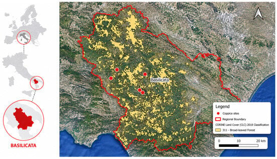
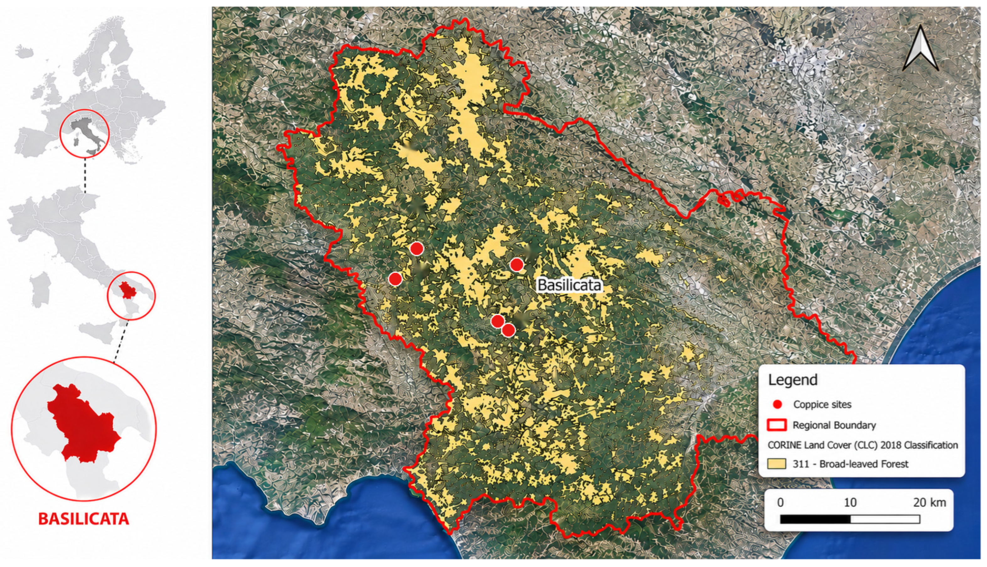
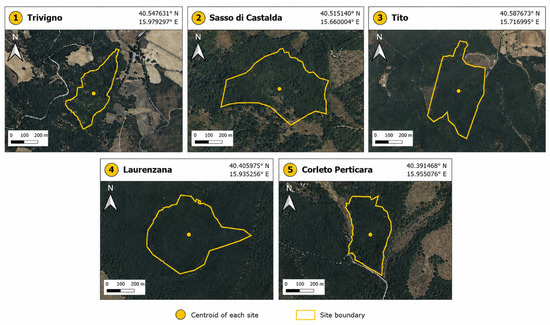
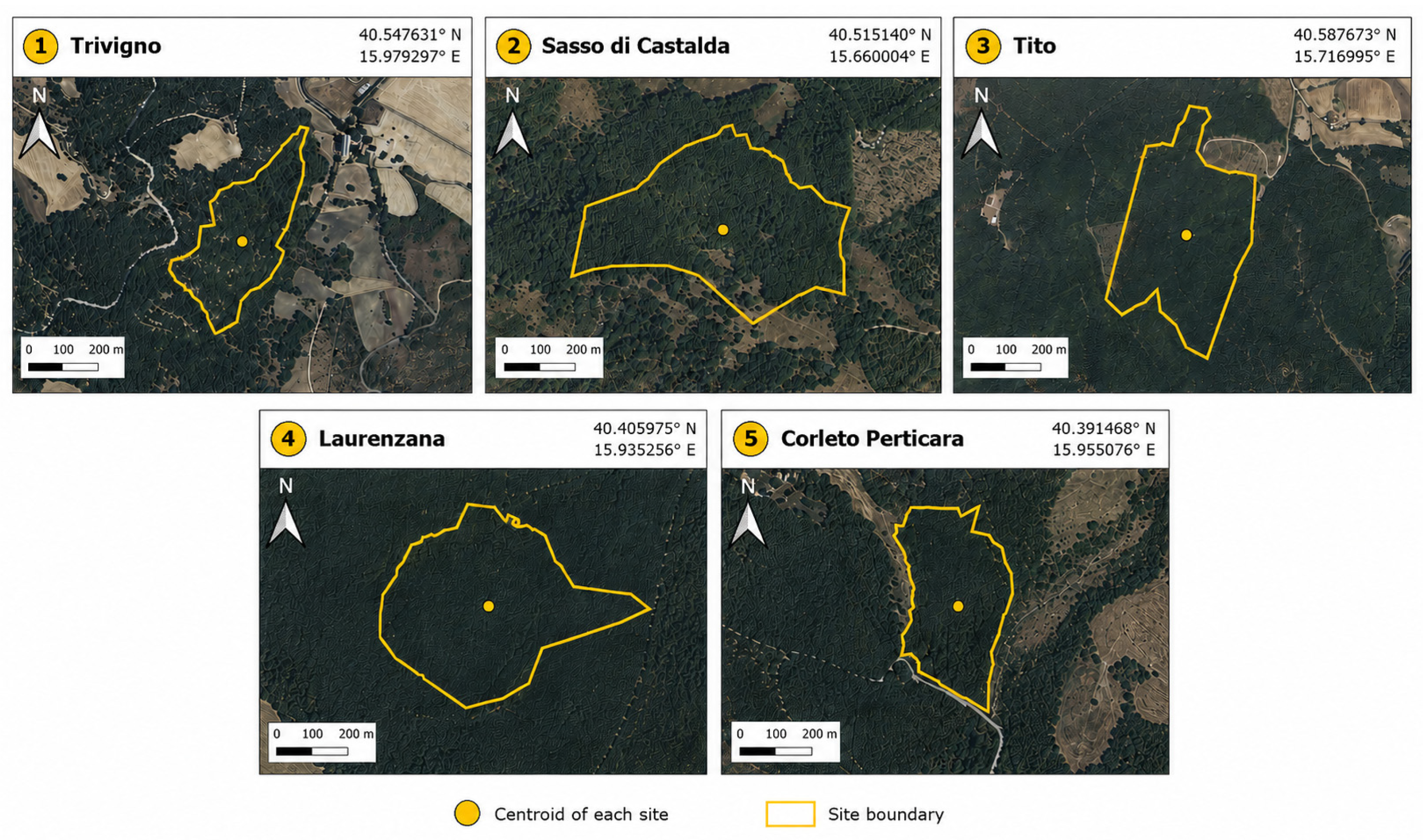
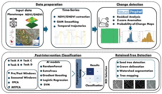
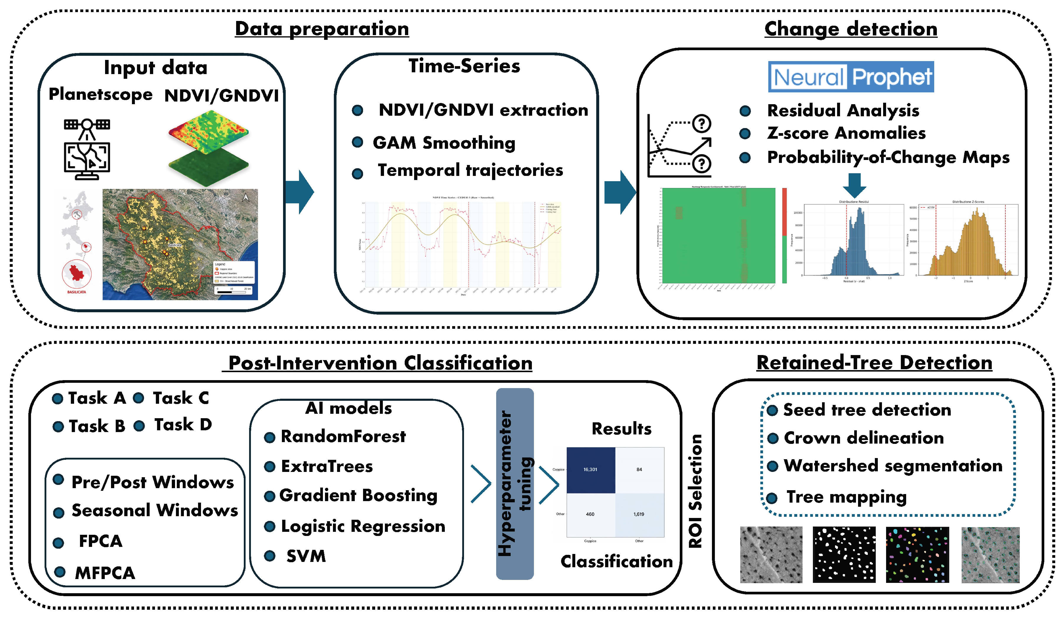
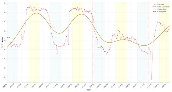
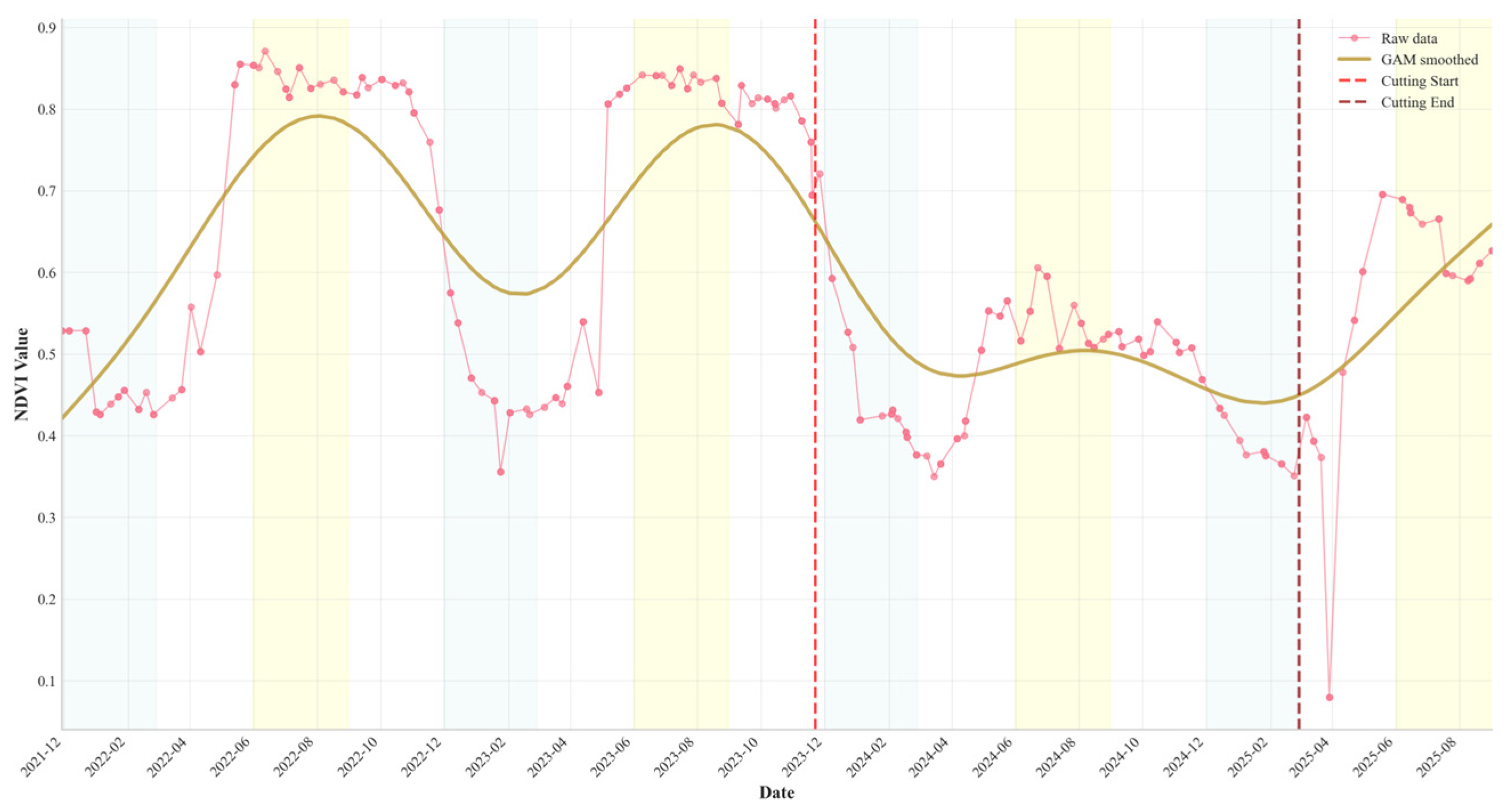
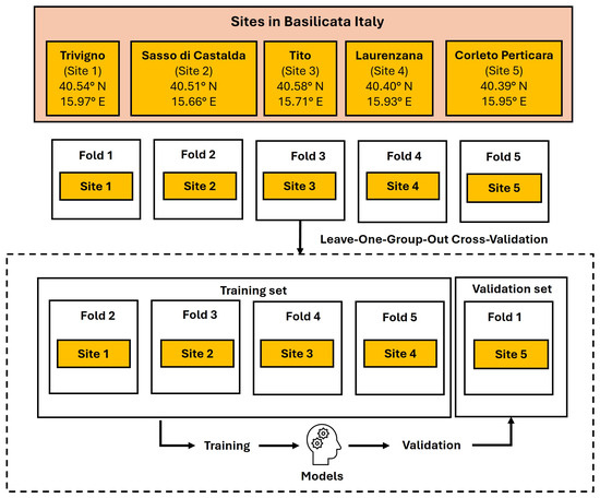
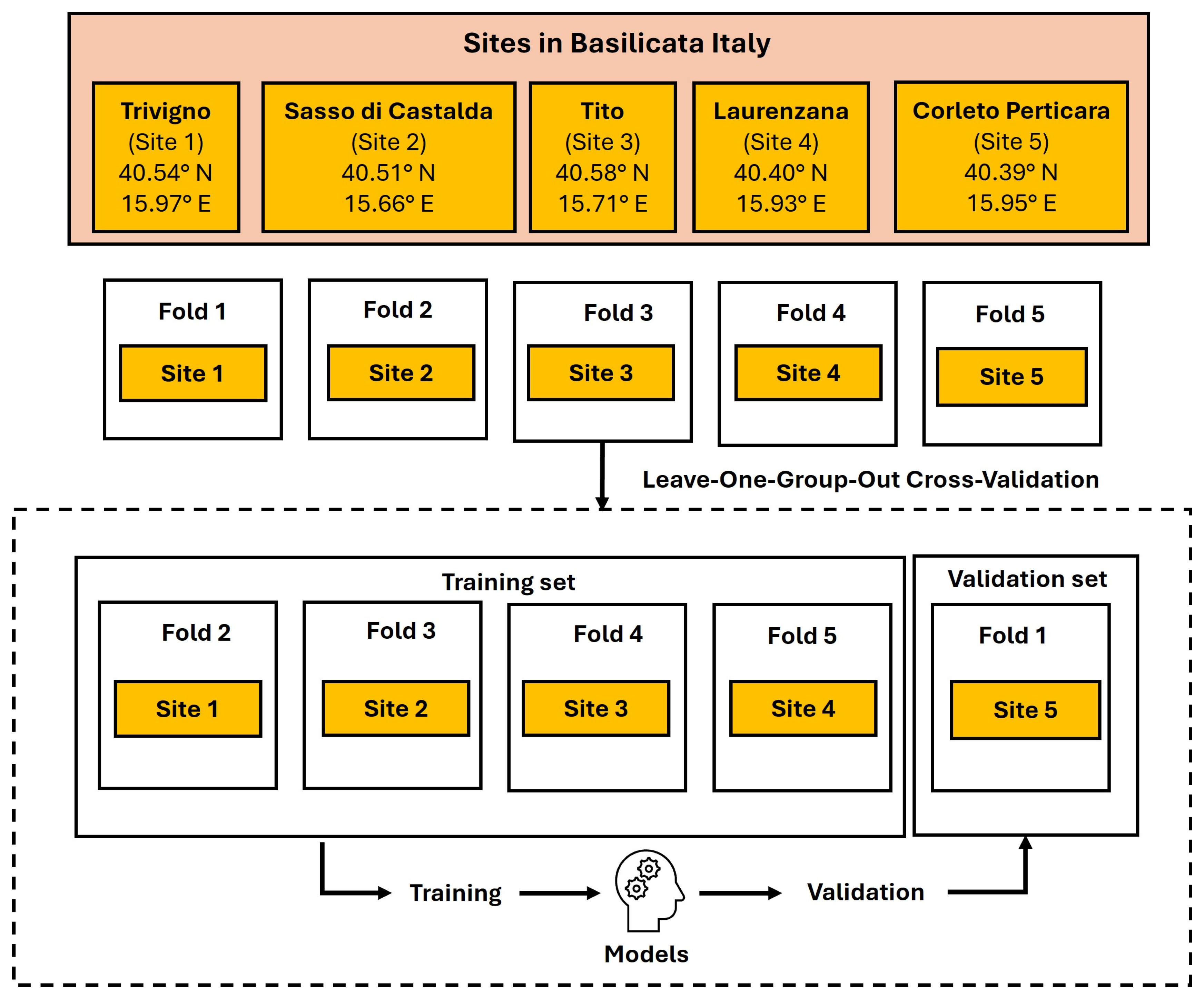
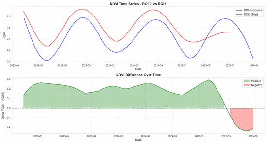
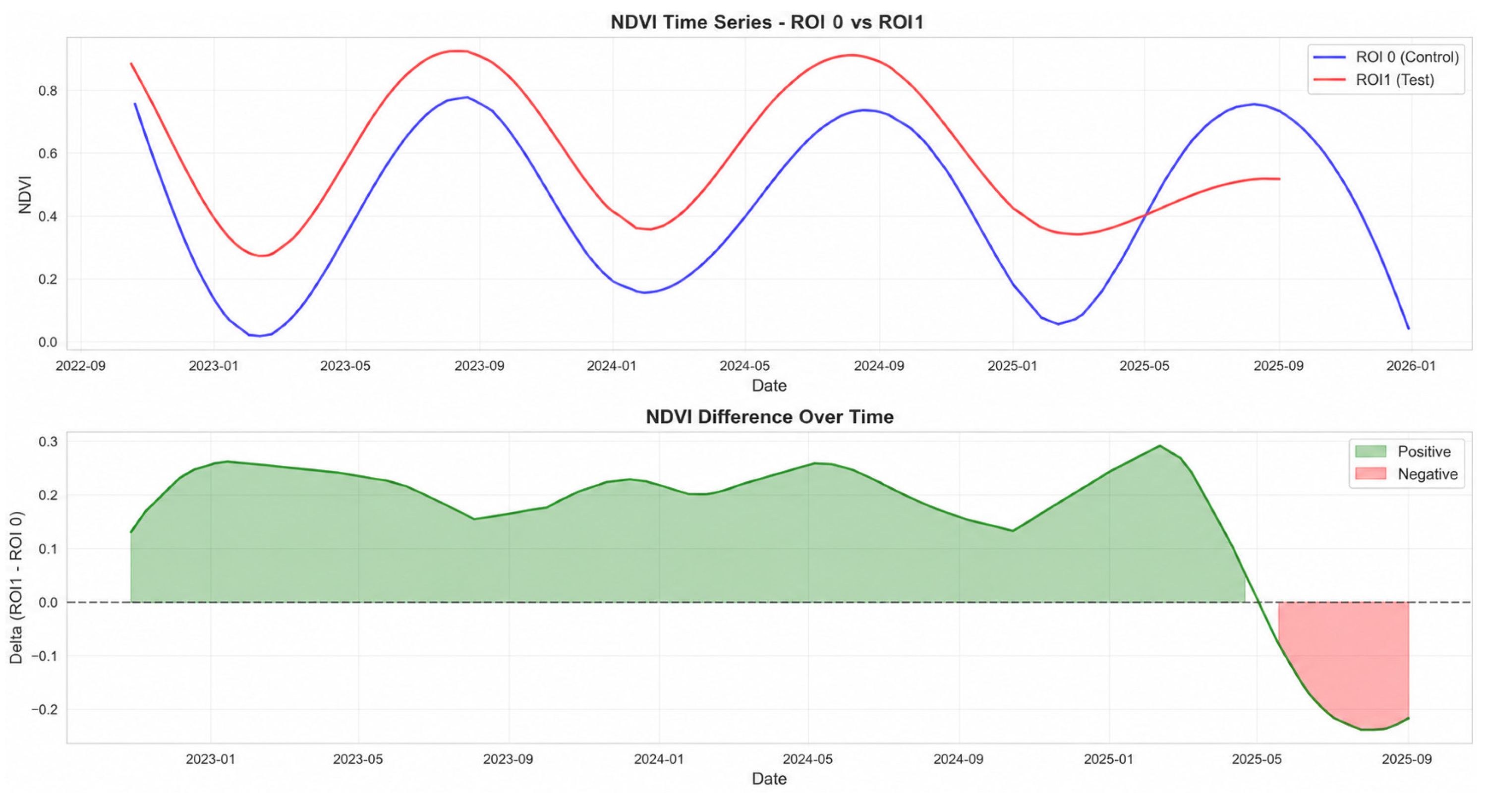
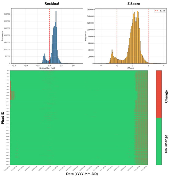
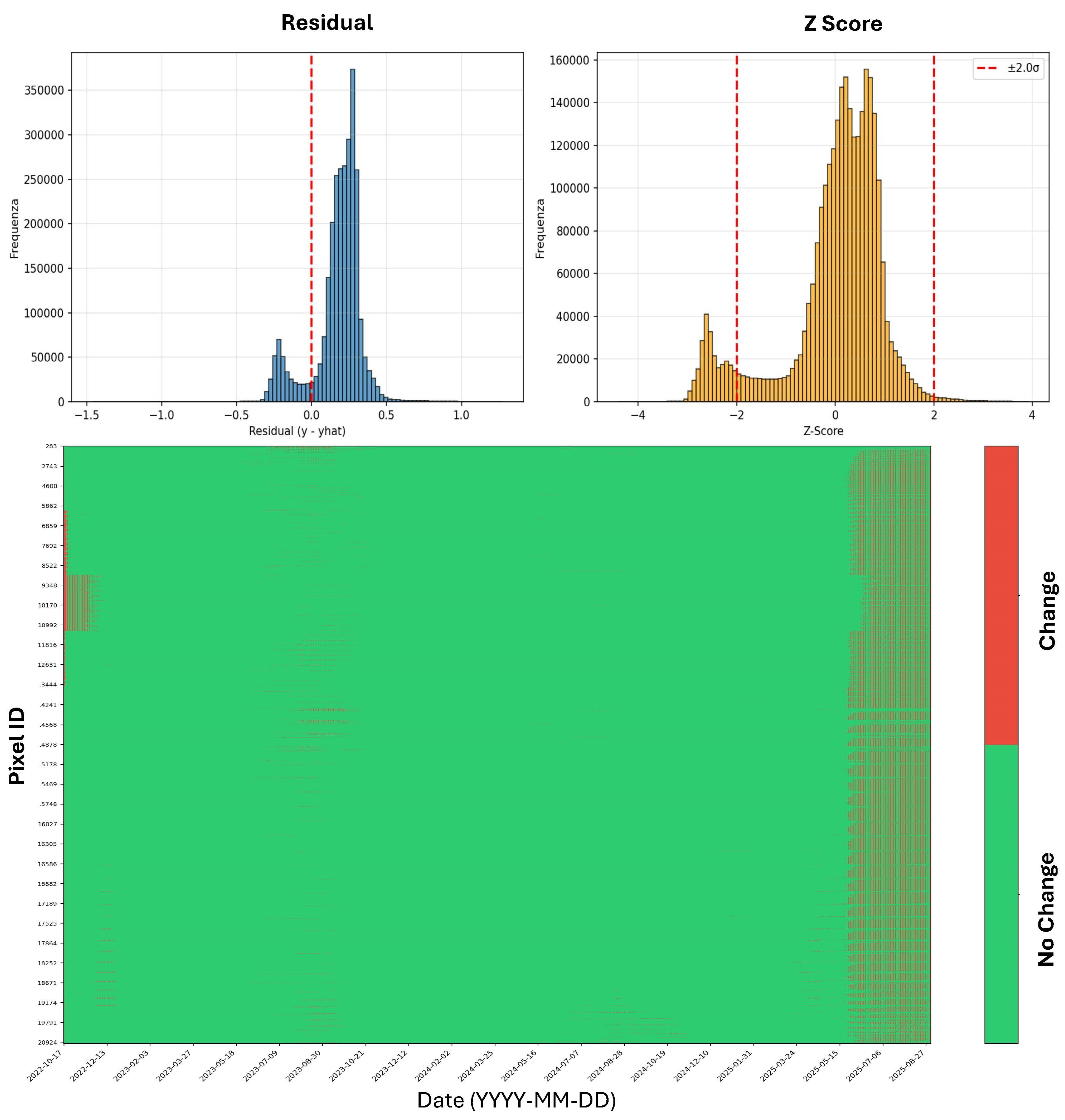
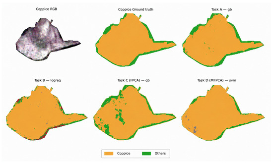
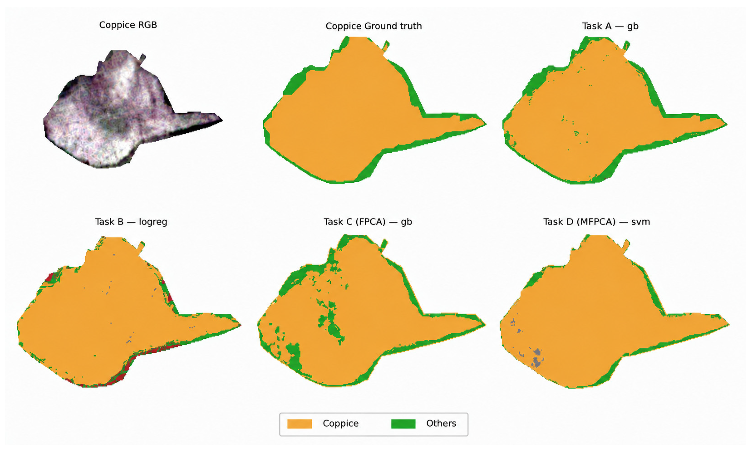
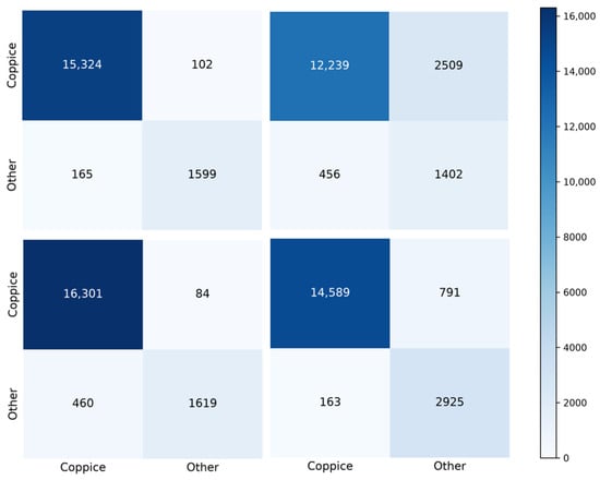
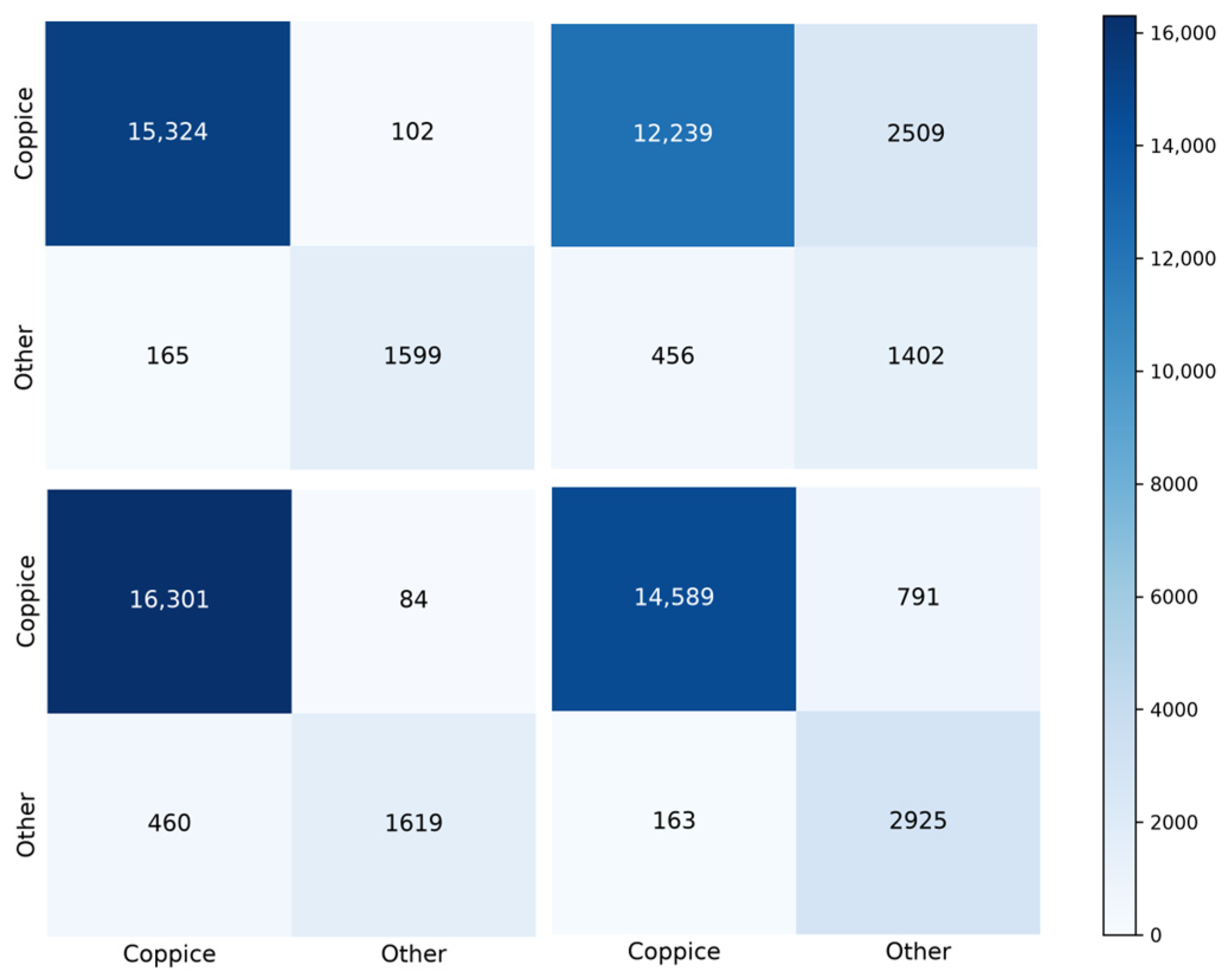
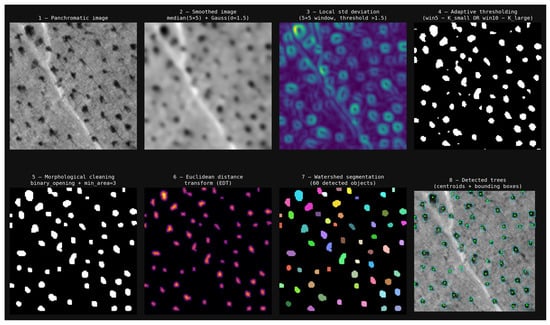
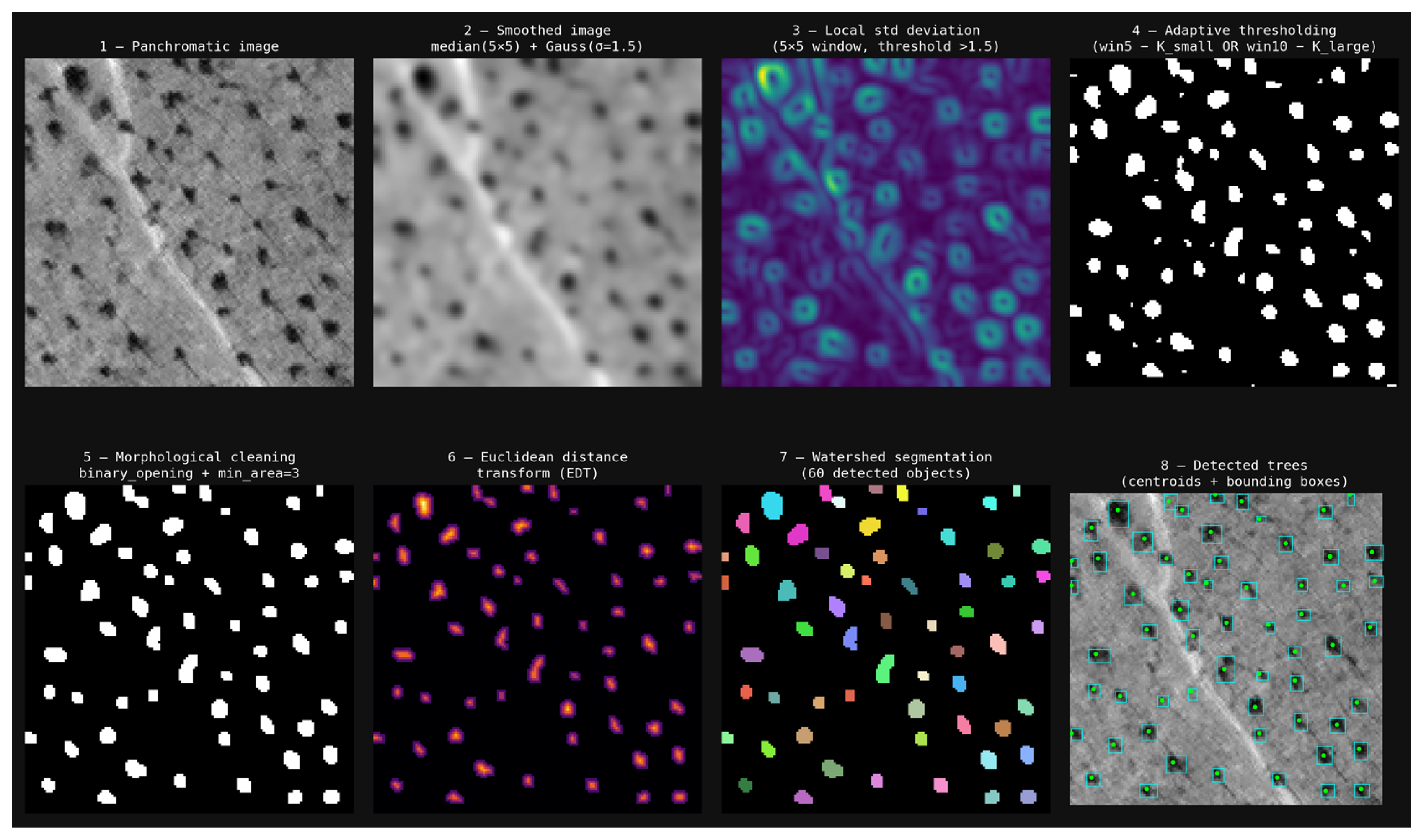

Disclaimer/Publisher’s Note: The statements, opinions and data contained in all publications are solely those of the individual author(s) and contributor(s) and not of MDPI and/or the editor(s). MDPI and/or the editor(s) disclaim responsibility for any injury to people or property resulting from any ideas, methods, instructions or products referred to in the content. |
© 2026 by the authors. Licensee MDPI, Basel, Switzerland. This article is an open access article distributed under the terms and conditions of the Creative Commons Attribution (CC BY) license.