


Highlights
What are the main findings?
- We propose a dual-domain representation learning method for few-shot HSIC. Its Euclidean encoder captures multi-scale long-range context through enlarged attention windows and cross-stage residual connections, while the spatial–spectral relation modeling module models spatial dependencies and spectral correlations in parallel to learn more discriminative representations.
- The method further incorporates geometric algebra representations, using an originalview branch to preserve information and a bidirectional guide-conditioned domain interaction module to facilitate dual-domain interaction. With only five labeled samples per class, it achieves overall accuracies of 77.15%, 84.63%, and 83.46% on the IP, PU, and Houston 2013 datasets respectively.
What are the implications of the main findings?
- Complementary learning between the Euclidean and geometric algebra domains provides an effective solution for HSIC with limited labeled samples.
- Our method demonstrates the potential of geometric algebra for few-shot HSIC.
Abstract
Few-shot hyperspectral image classification (FS-HSIC) remains highly challenging because the limited number of labeled samples not only makes traditional supervised learning models prone to overfitting but also restricts their ability to learn generalizable spatial–spectral representations. Moreover, existing methods are typically confined to a single Euclidean space and may therefore fail to capture complementary geometric structural information. Traditional contrastive learning based on two augmented views may also discard the information in the original samples that is essential for distinguishing different classes. To address these issues, we propose a dual-domain representation learning framework that jointly leverages complementary representations from the Euclidean and geometric algebra (GA) domains for FS-HSIC. In the Euclidean domain, we develop a multi-scale spatial–spectral residual Transformer (MSSRT) network that aggregates multi-scale long-range contextual information by progressively enlarging the attention windows and introducing cross-stage residual connections. A spatial–spectral relation modeling (SSRM) module further learns spatial dependencies and spectral channel correlations in parallel. In the GA domain, a spatial–spectral geometric algebra Transformer (SS-GATr) encodes hyperspectral features as multivectors and captures geometric information complementary to that represented in the Euclidean representations. During contrastive learning, an additional original-view branch is incorporated alongside two augmented-view branches, enabling the network to preserve fine-grained information while learning representations that are invariant to data augmentation. Furthermore, we propose a bidirectional guide-conditioned domain interaction (BGDI) module that selectively transfers information between the two domains based on inter-branch feature correlations, thereby facilitating the bidirectional exchange of complementary information while suppressing interference from irrelevant features. During few-shot finetuning and classification, the predictions of the two branches are weighted using a controllable fusion coefficient to balance the contributions of the two complementary representations when only limited labeled samples are available. Experiments are conducted on the Indian Pines, Pavia University, and Houston datasets using only five labeled samples per class. Compared with the state-of-the-art methods, the proposed method achieves overall accuracies (OAs) of 77.15%, 84.63%, and 83.46% on the three datasets, respectively, demonstrating the strong and competitive performance.
1. Introduction
Hyperspectral images (HSIs) capture the reflectance characteristics of ground objects across continuous and densely sampled spectral bands while preserving their spatial distribution, enabling accurate identification of different land-cover materials [1]. The rich information provided by hundreds of spectral bands has led to the widespread application of hyperspectral remote sensing in environmental monitoring, vegetation classification, geological and mineral identification, crop growth monitoring, and many other fields. However, acquiring high quality labeled samples requires expert-level knowledge and extensive field surveys, making it difficult to obtain sufficient training data. Therefore, effectively exploiting the information contained in limited labeled samples to achieve reliable few-shot hyperspectral image classification (FS-HSIC) remains an important challenge in the field of hyperspectral remote sensing.
In recent years, representative deep learning methods for hyperspectral image classification (HSIC) have included convolutional neural networks (CNNs) [2], Transformers [3], Mamba-based state space networks [4], hybrid neural network architectures [5], and hyperspectral foundation models [6]. However, traditional CNN methods rely on local convolutions. Although they can extract neighborhood textures and local spectral patterns, their ability to model dependencies between distant pixels is constrained by the limited kernel size [7]. Standard window-based Transformers introduce self-attention mechanisms, but their fixed windows still restrict the receptive field [8]. Moreover, most existing methods do not independently model spatial positional dependencies and spectral channel correlations in parallel, which may lead to mutual interference between spatial and spectral information. Consequently, the comprehensive extraction and complementary fusion of spatial structures and spectral information may be compromised. Recent Mamba-based architectures integrate pyramid spectral attention, adaptive expert depthwise convolution, and parallel spatial and spectral Mamba branches to capture multiscale spectral features, spatial structures, and long-range dependencies. However, HyPyraMamba [9] primarily focuses on efficient spatial–spectral sequence modeling in the Euclidean domain and does not exploit the complementary information available in the Euclidean and geometric algebra domains.
Existing FS-HSIC methods mainly include data augmentation [10], contrastive learning [11], transfer learning [12], and self-supervised learning [13]. Self-supervised and contrastive learning methods construct multiple augmented views from unlabeled samples. By bringing the representations of different views of the same sample closer together while separating those of different samples, these methods enable the model to learn transferable features before downstream classification [14]. Data augmentation methods promote feature invariance to transformations through operations such as spectral perturbation, spatial cropping, and noise injection. However, these operations may also weaken or even alter the original information relevant to class discrimination. Many two-view contrastive learning methods primarily focus on representation consistency between different augmented views, whereas the original samples are typically used only to generate these views and do not directly participate in representation learning through a separate, unaugmented branch. Consequently, the model may become biased toward adapting to variations introduced by augmentation and fail to fully preserve the spatial–spectral characteristics of the original samples. Therefore, it is necessary to preserve complete original information while achieving robustness to augmentation, thereby learning more stable and discriminative feature representations.
Currently, most HSIC methods generally extract spatial–spectral features within a single Euclidean space [15]. However, representations confined to a single Euclidean space may be insufficient to capture the complex geometric structures of hyperspectral data, particularly when labeled samples are scarce, thereby limiting the ability of the model to comprehensively represent discriminative features. Geometric algebra (GA) provides a unified framework for representing multidimensional geometric structures and is therefore particularly suitable for capturing the rich spectral–spatial relationships in HSI data [16]. Specifically, we represent hyperspectral features as GA multivectors. The geometric product jointly incorporates the inner product, which captures magnitude relationships, and the outer product, which characterizes oriented geometric structures, thereby establishing a unified algebraic framework for modeling high-dimensional spectral dependencies [17]. Interactive learning has shown its effectiveness in exploiting complementary information across different modalities or feature representations [18]. Nevertheless, effectively integrating information from the Euclidean and GA domains remains challenging because simple feature aggregation cannot adequately characterize the complementary relationships between the two representation spaces. When labeled samples are limited, indiscriminate information transfer may introduce unstable information from one branch into the other. Therefore, cross-domain fusion should not only enable feature exchange but also selectively enhance or suppress the features of the current branch according to the guidance provided by the other representation domain. Moreover, the two branches should complement each other bidirectionally from different representational perspectives.
To address the aforementioned issues, we propose a dual-domain representation learning framework for FS-HSIC. Our method consists of two stages: contrastive pretraining and few-shot classification. First, we design a Multiscale Spatial–Spectral Residual Transformer (MSSRT) network that employs multiscale residual Transformer (MRT) and a spatial–spectral relation modeling (SSRM) module to extract spatial–spectral features. Second, during contrastive pretraining, we introduce an additional branch for the original samples, allowing both the unaugmented original views and the augmented views to participate in representation learning. This design preserves the fine-grained information contained in the original hyperspectral data while learning representations invariant to data augmentation. We also apply GATr [19] to HSIC for the first time. It models hyperspectral features in the GA domain to capture structural information complementary to the features learned in the Euclidean domain. To effectively exploit information from the two representation domains, we further propose a Bidirectional Guide-Conditioned Domain Interaction (BGDI) module. Based on the feature correlations between the current branch and the guiding branch, BGDI selectively optimizes information transferred across the two domains and enables bidirectional interactions from the Euclidean domain to the GA domain and from the GA domain to the Euclidean domain. Finally, the two complementarily learned feature representations are fused during classification to obtain a richer and more comprehensive representation of HSIs. Experiments conducted on three representative datasets demonstrate the effectiveness and competitive performance of the proposed method when labeled samples are extremely limited. The main contributions of this paper are summarized as follows:
- We propose a dual-domain representation learning framework for FS-HSIC that jointly exploits complementary spatial–spectral representations in the Euclidean domain and multivector representations in the geometric algebra domain.
- We develop a triple-view contrastive learning strategy that combines one original view with two augmented views, preserving the fine-grained information of the original samples while learning invariance to data augmentation.
- We propose a bidirectional guide-conditioned domain interaction module that transfers and filters information according to feature correlations between the two representation domains, thereby enhancing the exchange of complementary information while suppressing interference from irrelevant features.
2. Related Work
2.1. Few-Shot HSI Classification
HSI classification typically relies on a large number of labeled samples. However, in real-world remote sensing scenarios, acquiring labeled data is costly, and only a limited number of training samples are available for each class. Therefore, few-shot learning (FSL) aims to train models with strong generalization capabilities to classify new samples using only a small number of labeled examples [20]. It should be noted that the FSL strategy adopted in this paper differs from traditional meta learning paradigms that use support and query sets [21]. Specifically, only a small number of labeled samples from each class are selected to train the model, while the trained model is used to classify the remaining samples not included in the training set. Existing methods for few-shot hyperspectral image classification (FS-HSIC) can be broadly divided into four categories: data augmentation, metric learning, transfer learning, and generative learning methods [22]. Furthermore, in recent years, foundation models pretrained on large remote sensing datasets have emerged as an important research direction in remote sensing representation learning. SpectralGPT [23] employs a three-dimensional generative pretraining mechanism to learn coupled spatial–spectral representations, whereas HyperSIGMA [24] is a foundation model with one billion parameters that jointly captures spatial and spectral features for diverse HSI understanding tasks. However, applying existing remote sensing foundation models to FS-HSIC still faces challenges, including the high cost of finetuning large models and the risk of overfitting when only a limited number of samples are available. Therefore, how to effectively leverage the general prior knowledge embedded in foundation models and achieve lightweight, task-adaptive transfer for FS-HSIC remains a promising research direction.
Data augmentation methods expand the training set by transforming a limited number of labeled samples or generating new samples, thereby improving the generalization ability of the model [10,25]. Yang et al. [26] proposed a deep transfer contrastive learning network (DTCLN) that generates augmented samples through random spectral shifts and Gaussian noise injection. This approach broadens the data distribution under few-shot conditions and increases sample diversity. Metric learning methods classify HSIs with limited labeled samples by learning similarity measures between samples. These methods bring similar samples closer together while pushing dissimilar samples farther apart [27]. Guo et al. [28] proposed a FS-HSIC method based on dynamic fusion and hierarchical enhancement. The method enhances the features of the support and query sets through intra-class self-attention and inter-class cross attention. It also optimizes the metric space by combining intra-class consistency loss with inter-class orthogonal loss, thereby promoting feature aggregation within classes and feature separation between classes. Xi et al. [29] proposed HyperTaFOR, a task-adaptive framework for few-shot open-set recognition that integrates a spatial–spectral selective Transformer with a negative prototype generation module. This method generates task-adaptive rejection scores to classify known categories and identify unknown samples. Transfer learning addresses the scarcity of labeled data by transferring knowledge learned from a source domain or a related task with abundant labeled samples to the target HSIC task [30]. Ma et al. [31] proposed an adaptive transfer framework called Interactive Spectral–Spatial Self-Supervised Learning (ISST-SSL). This framework pretrains spatial and spectral encoders separately and employs bidirectional interactive attention to dynamically align and integrate spatial and spectral knowledge across domains, thereby improving the model’s adaptability to the target domain and its classification robustness. Generative learning methods alleviate the shortage of labeled samples and improve classification performance by learning the distribution of hyperspectral data and generating realistic new samples [32]. Yang et al. [33] proposed a dual-branch mapping GAN with a Transformer, namely DMTF-GAN, which generates high-quality, diverse samples through noise grouping, label embedding, and dual-branch interaction with the Transformer. By utilizing a cross-layer adaptive fusion discriminator to preserve important feature information, it improves the classification performance of HSIs with a small number of training samples.
Unlike the FS-HSIC methods described above, our proposed method focuses more on enhancing the intrinsic feature representation capabilities of hyperspectral data. The designed MSSRT feature extraction network employs two parallel branches to model spatial dependencies and spectral correlations, respectively. Meanwhile, progressively enlarged attention windows capture both fine-grained local features and long-range contextual information, while multiscale residual connections help promote feature reuse, preserve shallow-layer information, and improve the stability of network training. The resulting spatial–spectral representations are then fed into a bidirectional cross-domain interaction module, where they interact bidirectionally with geometric multivector representations to obtain richer representations of hyperspectral data, thereby addressing HSI classification under limited labeled samples.
2.2. Feature Fusion Methods for HSI Classification
Feature fusion methods aim to integrate complementary information from different feature spaces, network branches, or representation scales to enhance the discriminative capability of HSI classification models [34]. Liu et al. [35] proposed a dynamic synchronous multiscale spectral–spatial graph convolutional network that highlights key spectral bands through a weighted spectral optimization module. By combining a CNN with adaptive dynamic graph convolution, the network extracts both local and long-range spectral–spatial features. Furthermore, it utilizes a bidirectional LSTM to fuse information across different scales, thereby improving the classification performance of HSIs with a small number of samples. Cao et al. [36] proposed a dual-branch manifold convolution-Mamba network (DBMCMamba), which uses an improved Mamba branch to adaptively fuse forward and backward information to model global dependencies. Through a manifold convolution branch, it jointly extracts local spectral–spatial features and second-order statistical features on the SPD manifold, and finally fuses global and local information to perform classification of HSIs with few samples. An et al. [37] proposed a Multiscale Interactive Attention Fusion Network (MIAF-Net), which uses CNNs and GCNs to extract local spatial features and global topological information, respectively. It employs a dual-branch interactive attention mechanism to facilitate the interaction of heterogeneous features and further utilizes a hierarchical attention mechanism to adaptively fuse information across different scales, thereby improving the performance of HSIC.
Although the aforementioned methods have improved HSI classification performance under limited sample conditions through graph learning or manifold representations, they still have certain limitations in the collaborative modeling of heterogeneous features. Our method learns spatial and spectral representations in the Euclidean domain and geometric multivector representations in the non-Euclidean domain, while establishing bidirectional interactions between the two domains. This enables Euclidean features and non-Euclidean geometric features to mutually guide and enhance each other, thereby facilitating a more comprehensive use of the complementary information contained in both representations. Consequently, more discriminative and robust hyperspectral features can be obtained when only a limited number of labeled samples are available.
2.3. Contrastive Learning for HSI Classification
Contrastive learning enhances feature discrimination by reducing the distance between semantically related samples and increasing that between unrelated samples in the embedding space [38]. Chen et al. [14] proposed supervised contrastive learning in prototypical networks, i.e., SCL-P-Net, which uses data augmentation to generate positive views of original samples and combines supervised contrastive loss with prototypical loss to constrain the clustering of similar samples and the separation of dissimilar samples, thereby enhancing the feature discriminative ability for classifying HSIs with a small sample size. Zhao et al. [15] proposed the Purified Contrastive Learning (PCL) framework, which downweights highly similar negative samples using superpixel-space priors to mitigate the interference of false negative samples on contrastive learning. Simultaneously, it combines CNNs and Transformers to extract local structures and global spectral–spatial information, thereby improving the performance of HSIC with limited labeled samples. Yang et al. [26] proposed the Deep Transfer Contrastive Learning Network (DTCLN), which utilizes an ImageNet pretrained model and a spectral residual network to extract and fuse spatial–spectral features. By combining spectral data augmentation, spatial attention, and supervised contrastive loss, the method enhances feature discriminative ability and classification performance when only limited labeled samples are available.
Although existing contrastive learning methods improve feature discrimination for FS-HSIC, they typically contrast only two augmented views without direct constraints from original samples, making them susceptible to spectral or spatial perturbations caused by data augmentation. Furthermore, diffusion-based contrastive learning methods, such as DiffCRN [39], learn spatial–spectral representations by combining iterative diffusion denoising with contrastive constraints and aggregating features across different diffusion timesteps. However, these methods are primarily confined to a single Euclidean representation space. In contrast, our framework incorporates one original view and two augmented views to construct triple-view contrastive constraints and jointly learns complementary representations in the Euclidean and geometric algebra domains. This design aims to preserve the fine-grained information of the original samples while exploiting augmentation invariance and cross-domain complementarity.
3. Materials and Methods
3.1. Framework Overview
The overall architecture of the proposed framework is illustrated in Figure 1, consisting of three stages of self-supervised pretraining, finetuning, and classification. The pretraining stage comprises a Euclidean spatial–spectral encoder, a geometric algebra (GA) representation encoder, and a bidirectional guide-conditioned domain interaction (BGDI) module. In the Euclidean spatial–spectral branch, a 3D convolution is first employed to compress the spectral dimension and extract local spatial–spectral features. Then the features are processed by a multiscale spatial–spectral residual Transformer (MSSRT), which jointly models spatial dependencies and inter-channel correlations within progressively enlarged windows. In parallel, the GA branch first employs a convolutional backbone to extract local features. The feature vector at each spatial location is then encoded as a multivector token and fed into a spatial–spectral geometric algebra Transformer (SS-GATr) to capture geometric relationships in the GA representation space. To facilitate complementary learning between the two representation spaces, BGDI is introduced prior to contrastive learning. Given a target representation to be updated and its complementary guidance representation, the module jointly exploits their normalized features, element-wise product, and absolute difference. These features are subsequently fed into a gating network composed of two fully connected layers to generate a weight for each embedding dimension. The resulting weight vector adaptively gates the value features in multi-head attention, followed by a residual connection to enhance the target representation. The two directional interactions are applied to the Euclidean spatial–spectral branch and the GA branch, respectively, thereby enabling bidirectional information transfer across the two representation spaces.
Figure 1.
Illustration of the proposed framework: (a) During self-supervised pretraining, the original HSI patch and two augmented views are encoded in the Euclidean and GA domains. BGDI enables cross-domain interaction, followed by pairwise SimCLR losses in each domain. (b) During finetuning, the pretrained encoders extract features from limited labeled samples. Two linear classifiers are trained with cross-entropy loss, and their outputs are weighted and fused for final prediction.
During pretraining, two randomly augmented views are generated for each input sample, while the original sample is retained as a third view. The three views are independently fed into the Euclidean spatial–spectral encoder and the GA representation encoder, yielding two sets of complementary feature representations. Within each representation space, contrastive learning is employed to constrain the relationships among the three views. Specifically, representations of different views derived from the same sample are pulled closer together to establish positive pairs, whereas representations from other samples in the same batch are treated as negative samples. This strategy simultaneously improves cross-view consistency and inter-sample discriminability. After pretraining, the backbone networks of the two encoders are transferred to their respective classification heads for finetuning. At this stage, the two branches are optimized independently using the cross-entropy loss. During the finetuning phase, the classification logits produced by the two branches are combined through weighted linear fusion to obtain the final prediction.
3.2. Data Preprocessing and Multi-View Generation
Let the original hyperspectral image (HSI) cube be denoted by , where H, W, and C denote the height, width, and number of spectral bands, respectively. For a central pixel , where and denote its row and column coordinates respectively, a local hyperspectral patch is extracted from . During the self-supervised pretraining stage, two independent random augmentations are applied to each HSI patch, while the original patch is retained as a third view. These three views are jointly used to construct the contrastive learning task:
where denotes the normalization operation, while and denote two independent data augmentation operations. We adopt the data augmentation module developed in [40]. Specifically, the original image patch is first randomly cropped to of its spatial dimensions and then resized to its original size using nearest-neighbor interpolation. Subsequently, the contrast and brightness are randomly adjusted within a limited range. Finally, the pixel values are normalized to the range . To ensure a consistent input range across the three views, the original view is normalized to match the augmented views. Among the three views, the two randomly augmented views are employed to enhance the robustness of the model to spatial variations and spectral perturbations, whereas the original view is retained to preserve the information of the original data.
3.3. Dual-Domain Spatial–Spectral Representation Learning Network
3.3.1. Multiscale Spatial–Spectral Residual Transformer (MSSRT)
As shown in Figure 2, the Multiscale Spatial–Spectral Residual Transformer (MSSRT) branch extracts hyperspectral features by modeling spatial–spectral relationships across multiple scales. Through progressively enlarged windows and residual connections, MSSRT overcomes the limited receptive field of conventional window-based Transformers and enables the comprehensive aggregation of long-range spatial–spectral information across multiple scales. Moreover, existing methods typically model spatial and spectral information using cascaded attention mechanisms, in which the modeling of one type of information depends on the output of the other [15]. This sequential design may limit the independent and comprehensive exploitation of the spatial structures and spectral characteristics inherent in hyperspectral data. To address this issue, we adopt a parallel attention architecture to model spatial dependencies and spectral correlations independently and simultaneously. As illustrated in Figure 2, MSSRT comprises a patch embedding module, a multiscale residual Transformer (MRT), and a spatial–spectral relationship modeling (SSRM) module.
Figure 2.
Detailed architecture of the proposed MSSRT. MSSRT consists of a patch embedding module, an MRT feature extraction network, and cascaded SSRM blocks.
The patch embedding module consists of a 3D convolutional unit and a 2D convolutional layer. The 3D convolutional unit employs convolutional kernels of different sizes to extract local spectral information, whereas the 2D convolutional layer captures local spatial structural information. Subsequently, a flattening operation transforms the feature map of size into a sequence of tokens. To encode the spatial position of each token, learnable positional embeddings are added to the token sequence.
To capture global dependencies within spatial and spectral features, we propose the MSSRT network, which comprises a multiscale residual Transformer (MRT) and spatial–spectral relationship modeling (SSRM) modules. Specifically, the MRT consists of four sequentially connected SSRM modules, whose attention windows progressively increase in size rather than remaining fixed. This design enables the network to capture fine-grained local details while gradually expanding its receptive field to aggregate richer spatial–spectral contextual information. In addition, residual connections are introduced across different modules to enlarge the effective receptive field. At each stage, the features produced by the SSRM modules are concatenated and projected through a convolution before being fed into the subsequent stage. The final residual connection further stabilizes the training process and preserves the original information, allowing each stage to integrate shallow and deep representations while preventing vanishing gradients. Formally, let the input feature map be denoted by , where d denotes the number of channels, and h and w denote the spatial height and width of the feature map respectively. The four SSRM modules are connected through progressive feature concatenation as follows:
where denotes the j-th SSRM module, denotes concatenation along the channel dimension, represents the projection operation consisting of a convolution followed by a activation, J denotes the total number of SSRM modules, denotes the input feature of the j-th SSRM module, and denotes the feature output by the j-th SSRM module. The output of the final stage is obtained through a residual connection with a fixed scaling factor as follows:
where is the fixed scaling factor. By preserving the initial representation, this architecture progressively aggregates spatial–spectral contextual information extracted using attention windows of different scales.
Each stage incorporates a SSRM module to separately capture feature dependencies along the spatial and channel dimensions. Given an input feature map , the feature extraction operation first splits along the channel dimension, after which two parallel branches are employed to generate coupled feature representations. Specifically, the upper branch captures spatial information through convolutional operations, whereas the lower branch captures spectral information through a convolutional block. These features are further decomposed into a query representation and a value representation . In the spatial relationship modeling branch, the value features are first spatially compressed, followed by the computation of spatial dependencies, thereby enabling spatial contextual relationships to be modeled within windows of different sizes:
where the query matrix and value matrix are obtained by fusing local spatial and spectral features, denotes the value matrix obtained by spatially compressing , d is the feature dimension of each attention head, and denotes the dynamic relative positional bias. denotes the spatial relation matrix, and denotes the features enhanced by spatial relations. In the channel relationship modeling branch, spectral dependencies are computed along the spectral dimension to explicitly model spectral correlation:
where denotes the number of spatial positions within the window, denotes the spectral-channel relation matrix, and denotes the spectrally enhanced representation obtained by aggregating the features weighted by the spectral-channel relation matrix.
The spatial and spectral relationship modeling branches aggregate spatial and spectral information, respectively, through matrix multiplication between the corresponding relation matrices and value features. The outputs of the two branches are subsequently concatenated and linearly projected. Each SSRM module performs a residual update based on correlation, followed by a feedforward residual update:
After the multiscale residual stage, layer normalization and global average pooling are applied to the output to obtain the spatial–spectral representation in the Euclidean domain.
Finally, is fed into the bidirectional cross-domain interaction module for further refinement under the guidance of the geometric multivector representation.
3.3.2. Spectral–Spatial Geometric Algebra Transformer (SS-GATr)
As shown in Figure 3, to complement the spatial–spectral feature representation in the Euclidean domain, we construct an SS-GATr network branch. This branch encodes the input into multivectors and employs GATr [19] modules to capture complex compositional relationships among them, thereby producing more discriminative features. Specifically, the input hyperspectral patch is first processed by convolutional and max-pooling layers to reduce the computational cost of multivector attention. Subsequently, a convolution is employed to map the resulting features at each spatial location to latent channels, which are further reorganized into 64 multivectors, each containing 16 geometric algebra components. The resulting multivector representation is expressed as
where each spatial location is treated as a token, and denotes the total number of spatial tokens. For each token, 64 denotes the number of multivector channels, and each multivector contains 16 geometric algebra components.
In general, a multivector can be expressed as a sum of geometric elements of different grades, including a scalar (grade 0), vectors (grade 1), bivectors (grade 2), trivectors (grade 3), and a pseudoscalar of the highest grade (grade t). For the geometric algebra adopted in this work, which is generated by four basis vectors , , , and , each multivector comprises components, corresponding to all possible basis blades generated by these four basis vectors.
Figure 3.
Structure of the proposed SS-GATr.
It should be noted that the raw spectral bands are not directly partitioned into fixed groups of 16. Instead, all spectral bands of the input HSI patch are first processed by the convolutional feature extraction backbone. At each spatial location, a convolution maps the extracted features to 64 latent multivector channels, each containing 16 components. Here, the number 16 is determined by the basis blades generated by the four basis vectors of the four-dimensional projective geometric algebra adopted in this work. It represents the number of components in each multivector rather than the grouping size of the raw spectral bands. In this manner, datasets with different numbers of spectral bands can be accommodated without discarding any input bands. The resulting multivector representation is then fed into the GATr model to extract geometric features:
where the attention mechanism facilitates information interaction among spatial tokens within each hyperspectral patch, denotes the number of output channels, and 16 is the dimensionality of each multivector. Subsequently, the output multivector features are mapped through a projection layer to obtain a compact geometric representation for subsequent cross-domain interaction.
3.4. Bidirectional Guide-Conditioned Domain Interaction (BGDI)
The Euclidean spatial–spectral branch and the geometric algebra branch extract complementary information from the same hyperspectral patch. Let and denote the Euclidean spatial–spectral representation and the geometric algebra representation, respectively. To facilitate cross-domain information exchange while preserving the distinct characteristics of each domain, we design a bidirectional guide-conditioned domain interaction (BGDI) module. This module uses the representation from one domain to generate adaptive weights for individual feature dimensions in the other domain. It then enhances the representation within each domain through residual updates scaled by learnable gating coefficients.
Given the current domain representation and the guiding domain representation , layer normalization is first applied to each representation. The two normalized representations and , their element-wise product , and their absolute difference are then concatenated along the feature dimension to construct a cross-domain relation descriptor:
where the element-wise product captures feature consistency between the two domains, whereas the absolute difference characterizes their representational discrepancy. The cross-domain relation descriptor is mapped through an MLP, followed by a sigmoid function, to generate guidance-conditioned feature weights:
where denotes the gating vector generated by the guiding domain. These weights control the extent to which individual feature dimensions in the current domain are retained or suppressed under the guidance of the other domain.
In the attention computation, the query , key , and value are all derived from the normalized current-domain representation:
where denotes the weight matrix of a bias-free linear projection. The resulting query, key, and value tensors are then rearranged into the multihead form:
where the current implementation employs attention heads, and is the feature dimension of each head. To match the multi-head value representation, the guidance vector is reshaped into a head-wise gating matrix as
The resulting gating matrix is applied exclusively to the value tensor . The attention operation is then defined as
where denotes the intermediate feature obtained by performing attention-based aggregation on the current domain under the guidance of the guiding domain , ⊙ denotes element-wise multiplication. The query , key , and value are derived from the current domain, while the guiding domain reweights the current-domain value tensor through the gating vector . The attention output is subsequently used to update the current-domain representation through a residual path with a learnable scaling coefficient :
subsequently, a feedforward network is employed to further perform nonlinear feature transformation:
where and are learnable parameters whose contribution strengths to the cross-domain-guided attention output and nonlinear update are progressively determined during optimization. denotes a cross-domain interaction function conditioned on the guiding domain and used to update the current domain . The above operations are performed bidirectionally without parameter sharing:
Both directions perform parallel computations using the values of and before interaction as inputs. Consequently, the geometric algebra representation guides the feature update of the Euclidean spatial–spectral representation, while the latter provides complementary information for updating the geometric algebra representation in the reverse direction. Finally, the two interacted representations and are separately normalized using the norm to obtain and . They are subsequently used as input representations for dual-domain contrastive pretraining.
This bidirectional guidance-conditioned representation interaction establishes conditional dependencies in both directions while preserving the specific domain information of the two representation spaces, thereby providing a feature representation that guides each other and maintains branch differences for subsequent comparative learning.
3.5. Triple-View Dual-Domain Contrastive Learning
To enable the dual-domain spatial–spectral feature representation network to learn consistent and complementary representations from different views of the same hyperspectral image patch, we design a triple-view dual-domain contrastive pretraining strategy. For each HSI patch, this strategy constructs two independently augmented views and one original reference view and imposes view-consistency constraints within both the Euclidean and GA domains. As described in Section 3.2, given an HSI patch , its three views are denoted by , , and .
The three views are separately fed into a dual-domain encoder network whose parameters are shared across the views:
where and denote the representations of the i-th sample from view t in the Euclidean and GA domains, respectively. Within the network, the two encoder branches first extract their domain-specific representations, after which complementary cross-domain information is exchanged through the BGDI module described in Section 3.4.
For a unified formulation of the domain-specific contrastive objectives, let
where E and G denote the Euclidean and GA domains, respectively, and denotes the representation of the i-th sample from view t in domain D.
For any two distinct views with , the representations of the same sample from views a and b within the same domain constitute a positive pair. The representations of the other samples in the batch are treated as negative samples. For the i-th sample, the contrastive loss from view a to view b in domain D is defined as
Here, N denotes the batch size, is the temperature parameter, and denotes the cosine similarity function. The numerator measures the similarity between two views of the same sample within the same representation domain. The denominator contains the other representations from views a and b, excluding only the anchor representation . Unlike traditional contrastive learning methods that use only two augmented views, our method imposes consistency constraints on all pairwise combinations of the three views:
denotes the overall contrastive loss between views a and b. The pair enforces consistency between the two randomly augmented views, whereas and anchor the two augmented views to the original reference view, respectively. This design reduces the dependency of the learned representations to specific augmentation perturbations and their random combinations, enabling the model to maintain more stable feature representations under varying augmentation conditions.
The sums of the three pairwise losses in the Euclidean and GA domains are defined as follows:
During pretraining, the Euclidean spatial–spectral branch and the GA branch first share complementary information through BGDI. Subsequently, the contrastive losses are computed independently within the two branches to enforce consistency among different views of the same sample in their respective representation spaces. The overall pretraining objective is defined as a weighted combination of the losses from the two domains:
Here, controls the relative contributions of the contrastive losses in the Euclidean and GA domains. The two domains employ the same triple-view pairing strategy, contrastive loss formulation, and temperature parameter while providing complementary spatial–spectral and geometric structural information, respectively. Therefore, equal weighting provides a symmetric optimization scheme without introducing an a priori preference for either representation domain. It should be noted that equal loss weights do not necessarily result in identical gradient contributions because the actual gradients also depend on the loss magnitudes, feature distributions, and parameter states of the two branches. The effects of different values of are further investigated in the parameter sensitivity analysis.
3.6. Supervised Transfer and Classification
After completing the triple-view dual-domain contrastive pretraining, we transfer the pretrained dual-domain encoder parameters to the downstream supervised classification network to leverage the spatial–spectral relationships learned during pretraining. In the supervised stage, the Euclidean spatial–spectral encoder and the GA encoder are retained, with a separate classification head assigned to each branch. In the current implementation, the BGDI module used during pretraining is removed, and the two pretrained encoders independently extract their respective features. This design not only enables cross-domain interaction using unlabeled data but also avoids finetuning additional parameters with limited labeled samples, thereby reducing the risk of overfitting. During finetuning, the Euclidean and GA branches are supervised independently using the class-weighted cross-entropy loss. Let and denote the classification logits produced by the Euclidean and GA branches for the i-th sample, respectively. The finetuning objective is defined as
where denotes the class-weighted cross-entropy loss and is the ground-truth label of the i-th sample. The contrastive pretraining objective is not jointly optimized with the classification loss during finetuning. Instead, it affects downstream classification by providing pretrained parameter initialization for the two encoders.
After supervised training, the class logits produced by the two branches are fused at the decision level using fixed weights:
where denotes the fused logit vector for the i-th sample, and i is the sample index. The scalar is a fixed fusion weight that control the contributions of the two branches to the final classification decision. A fixed fusion coefficient is adopted primarily because only five labeled samples are available for each class. With such extremely limited labeled data, introducing an additional adaptive fusion module may make the fusion weights more sensitive to sample selection and increase the risk of overfitting. Therefore, the fixed coefficient provides a simple and stable strategy for decision level fusion. The final class label is determined by the maximum response in the fused logits:
where denotes the final predicted class of the i-th sample. Here, k denotes the class index, and K is the total number of classes in the dataset. denotes the score of the k-th class in the fused logit vector , representing the model response for assigning the i-th sample to class k.
4. Experimental Results and Discussion
4.1. Datasets and Evaluation Metrics
4.1.1. Hyperspectral Datasets
To evaluate the classification performance of the proposed method across diverse scenarios, three publicly available HSI datasets were employed: Indian Pines (IP), Pavia University (PU), and Houston 2013 (Houston). Table 1 provides detailed information on the land-cover classes, along with the numbers of training and testing samples for each dataset.
Table 1.
Number of labeled samples per class used for finetuning and final testing on the three datasets.
The IP dataset was acquired in 1992 over northwestern Indiana, USA, using the Airborne Visible/Infrared Imaging Spectrometer (AVIRIS). After removing bands severely affected by noise and water absorption, 200 valid spectral bands were retained, covering a wavelength range of approximately . The image comprises pixels and contains 10,249 labeled pixels belonging to 16 land-cover classes. This dataset includes several crop classes with highly similar spectral responses, while some classes contain only a limited number of labeled samples. It is therefore well suited for evaluating classification performance under class-imbalanced conditions and for assessing the ability to discriminate spectrally similar fine-grained categories.
The PU dataset was acquired over the campus of the University of Pavia, Italy, using the Reflective Optics System Imaging Spectrometer (ROSIS). The image has a spatial size of pixels and comprises 103 valid spectral bands spanning approximately . It contains 42,776 labeled pixels distributed across nine land-cover classes. Compared with the IP dataset, PU exhibits more spatially continuous regions and more prominent urban structures. Nevertheless, several classes associated with construction materials show considerable spectral similarity. The dataset can thus be used to examine the ability of a model to characterize regional structures and preserve spatial boundaries.
The Houston 2013 dataset was acquired using the ITRES CASI-1500 sensor and was released for the 2013 IEEE GRSS Data Fusion Contest. It covers the campus of the University of Houston and the surrounding urban areas in the United States. The image has a spatial size of pixels and consists of 144 spectral bands covering a wavelength range of approximately . The dataset contains 15,029 labeled pixels from 15 land-cover classes. Its land-cover distribution is highly spatially heterogeneous, and several man-made objects exhibit similar spectral characteristics. Therefore, this dataset provides a challenging benchmark for evaluating the spatial–spectral discrimination capability of the proposed method in complex urban environments.
4.1.2. Evaluation Metrics
To comprehensively evaluate the classification performance of the proposed model across different class distributions and land-cover scenarios, we employ three widely used evaluation metrics: overall accuracy (OA), average accuracy (AA), and the Kappa coefficient (). OA is defined as the proportion of correctly classified samples among all test samples and is used to measure the overall classification performance of the model. AA is the arithmetic mean of the class-wise accuracies and provides a more balanced assessment of the model’s recognition performance across different classes, particularly when the class distribution is imbalanced. The Kappa coefficient measures the agreement between the predicted and ground-truth labels while correcting for agreement that may occur by chance. To reduce the effects of training sample selection, parameter initialization, and randomness in model optimization, each experiment was repeated independently 10 times. The results are reported as the mean ± sample standard deviation. To determine whether the observed performance differences were caused by random variation, we compared our method with PCL [15] because it is the most closely related baseline based on contrastive learning, using a two tailed Welch t test for independent samples based on the results of the 10 runs. This test does not require the two methods to have equal variances. The null hypothesis assumes that the two methods have equal population means for the corresponding evaluation metric, whereas the alternative hypothesis assumes that their population means are different. The significance level was set to . A difference was considered statistically significant when the two tailed p value was less than . Otherwise, the difference was regarded as numerical rather than statistically significant.
4.2. Experimental Setup
4.2.1. Implementation Specifications
For the IP, PU, and Houston datasets, a spatial neighborhood centered on each target pixel was extracted as the model input. This input patch size was determined based on the sensitivity analysis presented in Figure 4. The experiments followed a transductive self-supervised learning protocol. Using 50% of the samples for unlabeled pretraining provides sufficient data for self-supervised representation learning while ensuring a fair comparison with other methods that rely on pretraining by adopting the same data proportion. For each sample, two randomly augmented views and one original view were generated. The self-supervised pretraining split was generated independently of the downstream split into finetuning and test sets. During the supervised transfer stage, five labeled samples were randomly selected from each class for finetuning, while all remaining labeled pixels were treated as test samples, and their labels were accessed only for final evaluation. Therefore, the reported results reflect performance under a transductive protocol. The model was pretrained for 400 epochs using the Adam optimizer, with a batch size of 256 and an initial learning rate of . The model parameters obtained at the end of the 400th pretraining epoch were then loaded for supervised finetuning. Finetuning was performed for 300 epochs with a batch size of 64. These parameters were empirically determined based on preliminary experimental results, with consideration given to convergence stability and available computational resources. To mitigate the adverse effects of class imbalance, a class-weighted cross-entropy loss was employed, and the learning rate of the classifier was set to . The same implementation settings for the above experimental parameters were used across the IP, PU, and Houston datasets. All experiments were conducted on an NVIDIA GeForce RTX 4090 GPU using PyTorch 1.10.0 and Python 3.8.
Figure 4.
The impact of varying input patch sizes on OA across the IP, PU, and Houston datasets.
4.2.2. Baseline Method
To comprehensively evaluate the generalization capability of the proposed network in a setting with extremely limited labeled data, where only five labeled samples are available per class, we conducted both qualitative and quantitative comparisons with ten representative baseline methods. The selected competitors represent advanced baselines proposed in recent years and can be broadly categorized into three groups: self-supervised and contrastive learning methods, including L2CSL [40], C-SS-MTr [41], and PCL [15]; supervised learning methods, including 2D CNN [42], ViT [43], SSFTT [44], AMGCFN [45], DM-MRN [46], and SSEFN [47]; and a method based on a state space model, namely AdaMixCon [48]. To ensure a fair comparison, all baseline methods were configured using the parameter settings recommended in their original publications and evaluated using the same performance metrics. For methods involving a self-supervised or contrastive pretraining stage, including L2CSL, C-SS-MTr, PCL, and the proposed method, the same amount of unlabeled data was used for pretraining. Specifically, each method randomly selected 50% of the pixels from the same hyperspectral scenes as unlabeled pretraining samples. During the downstream supervised stage, all methods used five labeled samples per class for finetuning, while the remaining labeled samples were reserved for final testing. Each model was pretrained once, after which the resulting pretrained model was independently finetuned and tested over ten runs. Each finetuning run used a different random seed to independently control the random selection of labeled training samples and the initialization of model parameters. In contrast, the remaining supervised methods were trained from scratch using the same number of five labeled samples per class and independently trained and evaluated over ten runs.
4.3. Parameter Sensitivity Analysis
In the experiments, most parameters were set to fixed default empirical values. However, several important parameters were experimentally evaluated to determine their optimal values. During the finetuning stage, labeled samples were randomly selected from each class as training data. To evaluate the sensitivity of BGDI to the number of attention heads, we varied the number of attention heads on the IP dataset while keeping all other experimental settings unchanged. Specifically, the number of attention heads was set to 2, 4, 8, and 16. The experimental results in Table 2 show that the model achieved the highest OA with eight attention heads. The BGDI module is designed to capture complementary relationships between the two feature branches across multiple representation subspaces. These results indicate that too few attention heads limit the ability of BGDI to model cross-branch complementarity, whereas too many heads reduce the feature dimensionality assigned to each head and may introduce redundant attention information, particularly when only five labeled samples per class are available. For the image patch size, we tested , , , , and . The experimental results in Figure 4 demonstrate that a patch size of achieved the highest OA on the IP, PU, and Houston datasets. For the fusion coefficient , we tested values of , , , and . The experimental results in Table 3 show that the model achieved the highest OA when was set to . This indicates that the Euclidean domain representation provides the primary discriminative information, while the GA domain representation supplements it with geometric information. To investigate the effect of balancing the Euclidean-domain and GA-domain contrastive losses, we varied the pretraining loss weight over while keeping all other experimental settings unchanged. As reported in Table 4, achieves the best overall performance. This result supports the use of equal weighting for the two domain-specific contrastive losses and indicates that excessive emphasis on either representation domain may weaken the complementary learning between the Euclidean and GA branches.
Table 2.
Classification performance of BGDI with different numbers of attention heads on the IP dataset.
Table 3.
Classification performance of our method with different fusion coefficients on the IP dataset.
Table 4.
Classification performance of the proposed method with different pretraining loss weights on the IP dataset.
4.4. Experimental Results Analysis
4.4.1. Quantitative Analysis
Table 5, Table 6 and Table 7 summarize the classification results of different methods on the IP, PU, and Houston datasets, respectively. All results are reported as the mean ± sample standard deviation over 10 independent runs, and the best result in each row is highlighted in bold. Under the experimental setting with only five labeled samples per class, L2CSL, C-SS-MTr, PCL, and the proposed method, which employ pretraining or contrastive learning strategies, demonstrate strong overall competitiveness. Overall, the proposed method achieves the competitive performance on the three datasets. These results indicate that the proposed framework performs consistently well across both agricultural and urban hyperspectral scenes, although it does not achieve the best result for each metric on each dataset.
Table 5.
Classification Results of Different Methods on the IP Dataset.
Table 6.
Classification Results of Different Methods on the PU Dataset.
Table 7.
Classification Results of Different Methods on the Houston Dataset.
As shown in Table 5 and Table 8, on the IP dataset, the proposed method achieves an OA of , an AA of , and a value of , ranking first among all compared methods for all three overall evaluation metrics. Compared with PCL, the proposed method improves OA, AA, and by , , and percentage points, respectively. Statistical analysis further indicates that the improvements in OA and over PCL are statistically significant, with two-sided p-values of and , respectively. In contrast, the difference in AA is not statistically significant, with a two-sided p-value of . At the class level, the proposed method achieves classification accuracies of , , , and for Hay-windrowed, Wheat, Grass-trees, and Woods, respectively. These results demonstrate that the proposed method can effectively distinguish crop and vegetation classes with similar spectral characteristics. In addition, the hierarchical local windows, cross-stage residual connections, lightweight convolutions, and projections employed in MSSRT avoid the direct computation of attention among all tokens, thereby reducing computational overhead while retaining the ability to model multiscale contextual information.
Table 8.
Results of the one-sided and two-sided Welch’s independent-samples t-tests between the proposed method and PCL.
As shown in Table 6 and Table 8, on the PU dataset, the proposed method achieves an OA of , an AA of , and a value of . Its OA is percentage points lower than that of L2CSL, while its is percentage points lower. Nevertheless, compared with PCL, the proposed method improves OA and by and percentage points, respectively. These improvements are statistically significant, with two-sided p-values of for OA and for . The AA of the proposed method is percentage points lower than that of PCL, and the corresponding difference is not statistically significant, with a two-sided p-value of . For the individual classes, the proposed method achieves classification accuracies of , , , , and for Asphalt, Meadows, Gravel, Painted metal sheets, and Bare Soil, respectively. Although the proposed method does not achieve the best result for every class, its relatively high OA indicates favorable overall performance across repeated experiments.
As shown in Table 7 and Table 8, on the Houston dataset, the proposed method achieves an OA of , an AA of , and a value of . Among all the compared methods, the proposed method achieves the highest OA and , while its AA is only percentage points lower than the best result obtained by AdaMixCon. Compared with AdaMixCon, the proposed method improves OA and by and percentage points, respectively. Compared with PCL, it improves OA, AA, and by , , and percentage points, respectively. However, the results of the two-sided Welch’s t-test indicate that the differences between the proposed method and PCL in OA, AA, and are not statistically significant, with corresponding p-values of , , and , respectively. Therefore, these improvements should be interpreted as numerical improvements rather than statistically significant differences. At the class level, the proposed method achieves the highest classification accuracies of and for Residential and Road, respectively. Residential areas generally contain various land-cover components, such as buildings, roads, vegetation, and shadows, resulting in complex internal spatial structures. Meanwhile, Road can be easily confused with artificial surface classes such as Highway, Parking Lot 1, and Parking Lot 2. The favorable performance of the proposed method on these classes indicates that it can effectively exploit spatial contextual information to distinguish urban land-cover classes with similar spectral characteristics. In addition, the proposed method achieves classification accuracies of , , , and for Synthetic grass, Soil, Tennis Court, and Running Track, respectively.
Overall, the results presented in Table 5, Table 6 and Table 7 show that the proposed method achieves the best comprehensive performance on the IP dataset, competitive performance on the PU dataset, and the highest OA and on the Houston dataset. On the IP and PU datasets, the improvements in OA and over PCL are statistically significant, indicating that the observed performance gains are not entirely attributable to random experimental fluctuations. On the Houston dataset, although the proposed method obtains higher mean OA, AA, and values than PCL, the differences do not reach statistical significance. The IP dataset contains several crop classes with highly similar spectral responses, whereas the Houston dataset contains complex and spatially heterogeneous urban land-cover classes. The competitive performance achieved on these datasets indicates that the proposed dual-domain representation learning framework can adapt effectively to different hyperspectral classification scenarios.
Nevertheless, the classification results for some individual classes still exhibit relatively large standard deviations. This variability is mainly attributable to the use of only five labeled samples per class, which makes the classification results sensitive to training-sample selection, parameter initialization, and stochastic optimization. Furthermore, the Euclidean and GA branches exhibit different feature distributions and discriminative capabilities, and different land-cover classes may depend on the two branches to varying degrees. Since the fixed fusion coefficient cannot adaptively adjust the contribution of each representation domain for individual classes, the decision boundaries obtained across repeated runs may vary. Despite these limitations, the dual-domain complementary representations and the BGDI module generally enhance the discriminative capability of the model and alleviate the limitations associated with learning in a single representation space.
4.4.2. Visualization of Classification Results
To qualitatively evaluate the classification performance of different methods, Figure 5, Figure 6 and Figure 7 present the classification maps obtained by different methods on the IP, PU, and Houston datasets, respectively, together with the corresponding ground-truth maps and the overall accuracy of each method. The visual results are generally consistent with the quantitative results reported in Table 5, Table 6 and Table 7. Compared with the other methods, the classification maps generated by the proposed method generally exhibit better regional continuity, less intra-region noise, and higher consistency with the spatial distributions of the ground-truth labels. This may be attributed to the multiscale spatial–spectral contextual modeling of MSSRT, the extraction of geometric structural information in the GA domain by SS-GATr, and the selective interaction of complementary dual-domain information through BGDI. In addition, triple-view contrastive learning jointly utilizes the original view and two augmented views, thereby preserving fine-grained discriminative information from the original samples while enhancing representation robustness. Nevertheless, some misclassifications remain among classes with highly similar spectral characteristics, reflecting the difficulty of the classification task when only five labeled samples are available per class.
Figure 5.
Classification results obtained with different methods on the IP dataset (5 labeled samples for each class).
Figure 6.
Classification results obtained with different methods on the PU dataset (5 labeled samples for each class).
Figure 7.
Classification results obtained with different methods on the Houston dataset (5 labeled samples for each class).
As shown in Figure 5, the IP dataset contains several crop classes with similar spectral characteristics, including Corn-notill, Corn-mintill, Soybean-notill, Soybean-mintill, and Soybean-clean. Consequently, relatively evident class confusion and scattered noise can be observed in the classification maps generated by 2D CNN, ViT, and SSFTT. Although AMGCFN, DM-MRN, SSEFN, and AdaMixCon can identify the major agricultural regions, fragmented predictions remain in some corn and soybean fields. L2CSL and C-SS-MTr also exhibit evident confusion among crop classes with similar spectral responses. PCL produces relatively continuous results in some large agricultural fields, but local misclassifications remain in Corn-notill, Corn-mintill, and several soybean regions. In contrast, the proposed method better preserves the spatial distributions of the major agricultural fields and reduces scattered errors within crop regions, particularly exhibiting favorable spatial consistency in the Grass-trees, Hay-windrowed, Wheat, and Woods regions. These observations indicate that the complementary dual-domain representations facilitate the integration of local details, long-range contextual information, and geometric structural information, thereby improving the discrimination of spectrally similar crop classes. Some classification errors remain for classes with limited labeled samples, such as Alfalfa, Grass-pasture-mowed, Oats, and Stone-Steel-Towers, which is consistent with the relatively large performance variations observed for these classes.
Figure 6 presents the classification maps obtained by different methods on the PU dataset. This dataset contains large and spatially continuous urban regions, while classes such as Asphalt, Gravel, Bitumen, and Self-Blocking Bricks exhibit similar spectral characteristics. The classification maps generated by 2D CNN, ViT, and SSFTT contain relatively evident noise and boundary errors. Although AMGCFN, DM-MRN, L2CSL, C-SS-MTr, SSEFN, and AdaMixCon can recover the major spatial structures of the scene, local confusion remains among materials with similar spectral characteristics. PCL produces relatively coherent predictions in the Meadows, Painted metal sheets, and Bare Soil regions, but fragmented predictions remain in the Gravel, Trees, Self-Blocking Bricks, and Shadows regions. The proposed method effectively preserves the overall spatial layout of the scene and generates continuous predictions in the large Meadows and Bare Soil regions. It also exhibits favorable recognition performance for Painted metal sheets and other artificial surface classes. These observations indicate that the progressively enlarged attention windows expand the effective receptive field while preserving local boundary information, whereas BGDI selectively transfers complementary dual-domain information and suppresses interference from irrelevant features.
As shown in Figure 7, the Houston dataset contains urban land-cover classes with uneven spatial distributions and complex boundaries. The classification maps generated by 2D CNN, ViT, and SSFTT contain considerable scattered noise, particularly in regions containing roads, residential areas, commercial areas, and parking lots. AMGCFN and DM-MRN can recover some large and spatially continuous land-cover regions, but evident class confusion remains. L2CSL and C-SS-MTr improve the recognition of urban land-cover classes, although fragmented predictions are still observed near class boundaries. The classification maps produced by PCL and AdaMixCon are relatively coherent, but misclassifications remain among Road, Highway, Railway, Parking Lot 1, and Parking Lot 2. In contrast, the proposed method more accurately preserves the major spatial structures of Healthy grass, Stressed grass, Soil, Residential, and Road. In particular, the Residential and Road regions exhibit high consistency with the ground-truth labels. Residential areas generally comprise multiple land-cover components, such as buildings, vegetation, roads, and shadows, whereas Road can easily be confused with Highway and parking lots. By integrating multiscale spatial contextual information with geometric relationship information, the proposed method improves the representation of complex regional structures, class boundaries, and urban land-cover classes with intricate and interwoven spatial compositions.
Overall, the classification maps on the three datasets demonstrate that the proposed dual-domain framework can effectively integrate spatial–spectral features and geometric structural information. MSSRT captures local details and long-range contextual information, SS-GATr supplements the Euclidean-domain representations with geometric structural information, and BGDI facilitates selective bidirectional interaction between the two representation domains. Meanwhile, triple-view contrastive learning balances invariance to data augmentation with the preservation of original information, enabling the model to learn relatively stable and discriminative features even when labeled samples are extremely limited. Consequently, the proposed method exhibits favorable regional continuity and less intra-region noise in both agricultural and urban scenes. The remaining misclassifications are mainly concentrated in classes with highly similar spectral responses, complex boundaries, or limited labeled samples. These qualitative observations are generally consistent with the quantitative experimental results, further validating the effectiveness and scene adaptability of the proposed method for FS-HSIC.
4.4.3. Computational Complexity Analysis
To evaluate the computational efficiency of the proposed method, Table 9 reports the number of FLOPs and parameters of different methods on the Houston and IP datasets. On the Houston dataset, the proposed method achieves notable reductions in both FLOPs and parameter count compared with PCL [15]. Similarly, it requires fewer FLOPs and parameters on the IP dataset. This efficiency can be attributed to the hierarchical windows and parallel spatial–spectral relationship modeling employed by MSSRT, which avoid computationally expensive global self-attention. Moreover, lightweight convolutions and projections are used to control the feature dimensionality. Since the original and augmented views share the same feature encoder, the original-view branch introduces no additional model parameters. Overall, the proposed method effectively exploits the complementary information from the Euclidean and geometric algebra domains while maintaining moderate computational complexity and model size, thereby achieving a favorable balance between performance and efficiency.
Table 9.
Computational complexity of different methods on the Houston and IP datasets.
4.5. Ablation Study
4.5.1. Effect of Euclidean and Geometric Representations
The Euclidean and GA representation encoder jointly integrate spatial–spectral features in Euclidean space and structural features in the geometric algebra (GA) space. To evaluate the effectiveness of this dual-domain encoder for HSI classification with cross-domain interaction through the BGDI module, we conducted ablation experiments by removing the SS-GATr and MSSRT subnetworks on the IP and Houston datasets, denoted as w/o SS-GATr and w/o MSSRT, respectively. As reported in Table 10 and Table 11, the complete dual-domain encoder consistently achieves the best performance on both datasets. Specifically, on the IP dataset, the complete model improves OA by 4.25% and 4.68% compared with w/o SS-GATr and w/o MSSRT, respectively. On the Houston dataset, the corresponding OA improvements are 2.10% and 1.56%. Similar improvements can also be observed in terms of AA and . These results demonstrate that the Euclidean and GA domain representations provide complementary information. The MSSRT branch captures discriminative spatial–spectral features in Euclidean space, whereas the SS-GATr branch models additional structural relationships that cannot be sufficiently characterized using Euclidean features alone. Their interaction through BGDI therefore produces a more comprehensive and discriminative representation for HSI classification.
Table 10.
Ablation study of different components in the proposed method on the IP dataset.
Table 11.
Ablation study of different components in the proposed method on the Houston dataset.
4.5.2. Effect of Original View in Contrastive Learning
To investigate the role of the original-view branch in contrastive learning, we removed the third branch containing the original view while retaining the two augmented-view branches, denoted as w/o OSB. As reported in Table 10 and Table 11, removing the original-view branch consistently degrades classification performance on IP and Houston datasets. Specifically, compared with w/o OSB, the complete model improves OA, AA, and by 2.04%, 1.56%, and 2.22% on the IP dataset, respectively. On the Houston dataset, the corresponding improvements are 2.40%, 2.81%, and 2.58%. These results demonstrate that the original view provides a stable and reliable reference during contrastive learning, thereby facilitating the preservation of discriminative spatial–spectral information. Although the augmented views improve the robustness of feature representations to data perturbations, relying solely on them may cause the model to overemphasize representation consistency and consequently weaken the fine-grained information required to distinguish classes with similar spectral characteristics. Therefore, incorporating the original-view branch enables the model to better balance representation robustness and discriminative information preservation, leading to improved HSI classification performance when only limited labeled samples are available.
4.5.3. Effect of Bidirectional Guide-Conditioned Interaction
To validate the effectiveness of the proposed BGDI module, we compared three strategies: w/o Interaction, in which no interaction between the two representation domains was employed during contrastive pretraining and no interaction module was used during finetuning; w/ Cross-Attention, in which BGDI was replaced by standard cross-attention during contrastive pretraining, while the interaction module was removed during finetuning; and Ours, in which the proposed BGDI module was used during contrastive pretraining and removed during finetuning. As reported in Table 10 and Table 11, the absence of cross-domain interaction results in the lowest classification performance on both datasets, indicating that information exchange between the Euclidean and GA domain representations is beneficial for HSI classification. On the IP dataset, introducing standard cross-attention improves OA, AA, and by 0.69%, 0.74%, and 0.78%, respectively, compared with w/o Interaction. On the Houston dataset, the corresponding improvements are 1.84%, 1.12%, and 1.99%. Nevertheless, standard cross-attention remains inferior to BGDI. Compared with w/ Cross-Attention, BGDI further improves OA, AA, and by 3.46%, 0.91%, and 3.68% on the IP dataset and by 1.01%, 1.33%, and 1.09% on the Houston dataset, respectively. These results demonstrate that the bidirectional guidance and selective feature enhancement mechanisms of BGDI are more effective than standard cross-attention. Specifically, the guidance-conditioning mechanism enables each branch to selectively enhance informative features from the other representation domain while suppressing interference caused by inconsistent information. Overall, the experimental results demonstrate the effectiveness of BGDI in establishing mutually guided information interaction between the Euclidean and GA representation domains.
4.5.4. Effect of Retaining BGDI in the Finetuning Stage
To determine whether BGDI should also be retained during supervised finetuning, we compared two stage-wise configurations: Ours, in which BGDI was used only during contrastive pretraining and removed during finetuning, and BGDI+FT, in which BGDI was retained during both pretraining and finetuning. For BGDI+FT, the pretrained BGDI module was retained to generate the interacted representations in the Euclidean and GA domains. The two interacted representations were then fed into their respective classification heads, and the final logits were obtained using the same decision-level fusion strategy as in the proposed configuration. All other experimental settings were kept unchanged. As shown in Table 10 and Table 11, retaining BGDI during supervised finetuning leads to degraded classification performance on both datasets. On the IP dataset, Ours outperforms BGDI+FT by 3.29%, 2.63%, and 3.52% in terms of OA, AA, and , respectively. This performance gap is more pronounced on the Houston dataset, where Ours improves OA, AA, and by 5.12%, 4.77%, and 5.52%, respectively, compared with BGDI+FT. These results indicate that BGDI is more suitable for facilitating complementary cross-domain representation learning during contrastive pretraining than for direct application to few-shot supervised finetuning. During pretraining, abundant unlabeled samples provide relatively stable feature information for learning bidirectional interactions between the Euclidean and GA domains. In contrast, when only five labeled samples per class are available, retaining BGDI introduces additional trainable interaction parameters and tightly couples the two representation branches, making the model more sensitive to the selection of training samples and parameter initialization while increasing the risk of overfitting. Removing BGDI during finetuning allows the two pretrained encoders to adapt independently to the downstream classification task. Meanwhile, decision-level fusion preserves the complementary contributions of the two representation domains without introducing additional feature-level interactions. Therefore, applying BGDI only during contrastive pretraining provides a more effective and stable stage-wise strategy for FS-HSIC.
4.6. Effects of Labeled Training Sample Numbers
To investigate the classification performance of the proposed model with different numbers of training samples, we randomly selected 5, 10, 15, and 20 labeled samples from each class of the IP, PU, and Houston datasets for training. As illustrated in Figure 8, the OA values of all methods generally increase as more labeled samples become available, confirming the importance of labeled data for training deep learning classification models. Nevertheless, the proposed method achieves competitive OA with different numbers of labeled samples. It obtains the highest OA on the IP and Houston datasets under the evaluated settings and remains competitive on the PU dataset. Compared with SSEFN and AdaMixCon, which are designed for limited labeled samples, the proposed method also demonstrates favorable classification performance when the same number of labeled samples is used. These results demonstrate that the proposed method can effectively learn discriminative representations from limited labeled data and maintains relatively stable classification performance with different numbers of training samples.
Figure 8.
The impact of varying numbers of training samples on OA across the three datasets. (a) IP, (b) PU, and (c) Houston dataset.
5. Conclusions
This paper proposes a dual-domain representation learning method that integrates the Euclidean and GA domains based on triple-view contrastive learning. The method employs a multi-scale spatial–spectral residual Transformer (MSSRT) network to learn the spatial–spectral features of HSIs in Euclidean space and introduces geometric algebra representations into FS-HSIC to acquire complementary information from different representation domains. During contrastive learning, the branch processing the original view participates in representation learning together with two branches processing augmented views. This strategy helps preserve the original semantic information of the samples and encourages the same sample to have similar feature representations across the original and augmented views. Furthermore, the proposed bidirectional guide-conditioned domain interaction (BGDI) module selectively transfers information between the two domains according to the feature correlations between their branches, thereby enabling complementary bidirectional interaction while reducing interference from irrelevant information. During finetuning and classification, the classification outputs of the Euclidean and GA branches are fused in a weighted manner to integrate complementary discriminative information provided by the two types of representations. Extensive experiments on three benchmark datasets demonstrate that the proposed method achieves strong and competitive classification performance when labeled samples are extremely limited.
The proposed method achieves promising performance in FS-HSIC tasks, but it still has several limitations. First, the current experiments follow a transductive self-supervised learning setting, in which the data splits for self-supervised pretraining and those for downstream finetuning and testing are generated independently. Consequently, some downstream test pixels may have been used as unlabeled inputs during pretraining, although their class labels are used exclusively for final performance evaluation. Second, the proposed method requires relatively long training and inference times. Moreover, when the data are affected by different types of noise or exhibit substantial distributional differences, whether existing data augmentation strategies can consistently generate effective views suitable for contrastive learning remains to be further investigated. Finally, compared with remote sensing foundation models pretrained on massive datasets collected from multiple regions, the proposed model remains limited in terms of the scale of its pretraining data and its ability to generalize across datasets. Future work will further explore how to integrate hyperspectral self-supervised learning with remote sensing foundation models. For example, foundation models could provide general parameter initialization, while the proposed dual-domain contrastive learning mechanism could further enhance the model’s representations of spectral, spatial, and geometric structural features. Meanwhile, the model’s generalization performance will be further evaluated on more datasets, with different proportions of labeled samples, and across different scenes.
Author Contributions
Conceptualization, R.Z.; methodology, R.Z.; software, R.Z.; investigation, R.Z.; funding acquisition, W.C.; data curation, R.Z.; writing—original draft preparation, R.Z.; writing—review and editing, W.C., Q.L. All authors have read and agreed to the published version of the manuscript.
Funding
This research was funded by the Fundamental Research Foundation of Shenzhen, grant number JCYJ20230808105705012, and the China Postdoctoral Science Foundation, grant number GZC20240652.
Data Availability Statement
The data used in this study were obtained from publicly accessible data sources. The processed data and other materials supporting the findings of this study are available from the corresponding author upon reasonable request. The Indian Pines, Pavia University, and Houston 2013 datasets are available at https://doi.org/10.4231/R7RX991C, https://huggingface.co/datasets/Tanishq165/HSI_Datasets/tree/main/Pavia%20University, and https://machinelearning.ee.uh.edu/2013-ieee-grss-data-fusion-contest/, respectively. All datasets were accessed on 27 September 2026.
Acknowledgments
During the preparation of this manuscript, the authors used GPT-5.6-Sol for English language editing, including grammar checking, improving sentence clarity, and generating LaTeX code for table formatting. The authors carefully reviewed, verified, and revised the output generated by the tool and take full responsibility for the content of this publication.
Conflicts of Interest
The authors declare no conflicts of interest.
References
- Wu, G.; Al-Qaness, M.A.; Al-Alimi, D.; Dahou, A.; Abd Elaziz, M.; Ewees, A.A. Hyperspectral image classification using graph convolutional network: A comprehensive review. Expert Syst. Appl. 2024, 257, 125106. [Google Scholar] [CrossRef] [Scilit]
- Gong, Z.; Zhong, P.; Yu, Y.; Hu, W.; Li, S. A CNN with multiscale convolution and diversified metric for hyperspectral image classification. IEEE Trans. Geosci. Remote Sens. 2019, 57, 3599–3618. [Google Scholar] [CrossRef] [Scilit]
- Fu, C.; Zhou, T.; Guo, T.; Zhu, Q.; Luo, F.; Du, B. CNN-Transformer and Channel-Spatial Attention based network for hyperspectral image classification with few samples. Neural Netw. 2025, 186, 107283. [Google Scholar] [CrossRef] [Scilit] [PubMed]
- Zhang, H.; Liu, H.; Shi, Z.; Mao, S.; Chen, N. ConvMamba: Combining Mamba with CNN for hyperspectral image classification. Neurocomputing 2025, 652, 131016. [Google Scholar] [CrossRef] [Scilit]
- Ali, M.S.M.; Islam, M.S.B.; Majid, M.E.; Kashem, S.B.A.; Khandakar, A.; Chowdhury, M.E. A hybrid 3D CNN-LSTM model with soft spatial attention mechanism for accurate hyperspectral image classification. Remote Sens. Appl. Soc. Environ. 2025, 40, 101779. [Google Scholar] [CrossRef] [Scilit]
- Braham, N.A.A.; Albrecht, C.M.; Mairal, J.; Chanussot, J.; Wang, Y.; Zhu, X.X. Spectralearth: Training hyperspectral foundation models at scale. IEEE J. Sel. Top. Appl. Earth Obs. Remote Sens. 2025, 18, 16780–16797. [Google Scholar] [CrossRef] [Scilit]
- Hasan, M.A.; Bhargav, T.; Sandeep, V.; Reddy, V.S.; Ajay, R. Image classification using convolutional neural networks. Int. J. Mech. Eng. Res. Technol. 2024, 16, 173–181. [Google Scholar]
- Wang, Y.; Deng, Y.; Zheng, Y.; Chattopadhyay, P.; Wang, L. Vision transformers for image classification: A comparative survey. Technologies 2025, 13, 32. [Google Scholar] [CrossRef] [Scilit]
- Li, D.; Bhatti, U.A.; Huang, M.; Bruzzone, L.; Li, J. HyPyraMamba: A pyramid spectral attention and mamba-based architecture for robust hyperspectral image classification. IEEE Trans. Geosci. Remote Sens. 2026, 64, 5501016. [Google Scholar] [CrossRef] [Scilit]
- Wei, W.; Tong, L.; Guo, B.; Zhou, J.; Xiao, C. Few-shot hyperspectral image classification using relational generative adversarial network. IEEE Trans. Geosci. Remote Sens. 2024, 62, 5539016. [Google Scholar] [CrossRef] [Scilit]
- Xie, H.; Zhao, X.; Yin, J.; Peng, J.; Wang, Q.; Vivone, G. Cross-Architecture Contrastive Learning for Few-Shot Hyperspectral Image Classification. IEEE Trans. Geosci. Remote Sens. 2026, 64, 5504615. [Google Scholar] [CrossRef] [Scilit]
- Zhou, H.; Wang, X.; Xia, K.; Ma, Y.; Yuan, G. Transfer learning-based hyperspectral image classification using residual dense connection networks. Sensors 2024, 24, 2664. [Google Scholar] [CrossRef] [Scilit] [PubMed]
- Ma, S.; Tong, L.; Zhou, J.; Yu, J.; Xiao, C. Self-supervised spectral–spatial graph prototypical network for few-shot hyperspectral image classification. IEEE Trans. Geosci. Remote Sens. 2023, 61, 5518915. [Google Scholar] [CrossRef] [Scilit]
- Chen, L.; Wu, J.; Xie, Y.; Chen, E.; Zhang, X. Discriminative feature constraints via supervised contrastive learning for few-shot forest tree species classification using airborne hyperspectral images. Remote Sens. Environ. 2023, 295, 113710. [Google Scholar] [CrossRef] [Scilit]
- Zhao, L.; Li, J.; Luo, W.; Ouyang, E.; Wu, J.; Zhang, G.; Li, W. Purified contrastive learning with global and local representation for hyperspectral image classification. IEEE Trans. Geosci. Remote Sens. 2024, 62, 5520414. [Google Scholar] [CrossRef] [Scilit]
- Wang, R.; Ye, X.; Huang, Y.; Ju, M.; Xiang, W. GASSF-Net: Geometric algebra based spectral-spatial hierarchical fusion network for hyperspectral and LiDAR image classification. Remote Sens. 2024, 16, 3825. [Google Scholar] [CrossRef] [Scilit]
- Liu, Y.; Luo, Y.; Wang, R.; Huang, Y.; Ju, M.; Xiang, W. A geometric algebra-based model for enhanced hyperspectral anomaly detection. IEEE Trans. Geosci. Remote Sens. 2025, 63, 5517817. [Google Scholar] [CrossRef] [Scilit]
- Li, J.; Zheng, K.; Li, Z.; Gao, L.; Jia, X. X-shaped interactive autoencoders with cross-modality mutual learning for unsupervised hyperspectral image super-resolution. IEEE Trans. Geosci. Remote Sens. 2023, 61, 5518317. [Google Scholar] [CrossRef] [Scilit]
- Brehmer, J.; De Haan, P.; Behrends, S.; Cohen, T.S. Geometric algebra transformer. Adv. Neural Inf. Process. Syst. 2023, 36, 35472–35496. [Google Scholar] [CrossRef] [Scilit]
- Zhang, R.; Cao, W.; Liu, Q. Geometric algebra enhanced twin-branch contrastive network design for few-shot hyperspectral image classification. Pattern Recognit. 2026, 179, 113549. [Google Scholar] [CrossRef] [Scilit]
- Tian, J.; Wan, R.; Li, Z.; Wang, Y.; Fang, Z.; Guo, J.; Qi, M. A Multi-modal Prototype Correction and Multi-dimensional Knowledge Distillation Framework for Cross-domain Few-shot Hyperspectral Image Classification. IEEE Trans. Geosci. Remote Sens. 2025, 63, 5522718. [Google Scholar] [CrossRef] [Scilit]
- Wambugu, N.; Chen, Y.; Xiao, Z.; Tan, K.; Wei, M.; Liu, X.; Li, J. Hyperspectral image classification on insufficient-sample and feature learning using deep neural networks: A review. Int. J. Appl. Earth Obs. Geoinf. 2021, 105, 102603. [Google Scholar] [CrossRef] [Scilit]
- Hong, D.; Zhang, B.; Li, X.; Li, Y.; Li, C.; Yao, J.; Yokoya, N.; Li, H.; Ghamisi, P.; Jia, X.; et al. SpectralGPT: Spectral remote sensing foundation model. IEEE Trans. Pattern Anal. Mach. Intell. 2024, 46, 5227–5244. [Google Scholar] [CrossRef] [Scilit] [PubMed]
- Wang, D.; Hu, M.; Jin, Y.; Miao, Y.; Yang, J.; Xu, Y.; Qin, X.; Ma, J.; Sun, L.; Li, C.; et al. HyperSIGMA: Hyperspectral intelligence comprehension foundation model. IEEE Trans. Pattern Anal. Mach. Intell. 2025, 47, 6427–6444. [Google Scholar] [CrossRef] [Scilit] [PubMed]
- Wang, X.; Liu, J.; Chi, W.; Wang, W.; Ni, Y. Advances in hyperspectral image classification methods with small samples: A review. Remote Sens. 2023, 15, 3795. [Google Scholar] [CrossRef] [Scilit]
- Yang, G.; Wang, Z. A deep transfer contrastive learning network for few-shot hyperspectral image classification. Remote Sens. 2025, 17, 2800. [Google Scholar] [CrossRef] [Scilit]
- Jia, S.; Jiang, S.; Lin, Z.; Li, N.; Xu, M.; Yu, S. A survey: Deep learning for hyperspectral image classification with few labeled samples. Neurocomputing 2021, 448, 179–204. [Google Scholar] [CrossRef] [Scilit]
- Guo, Y.; Fan, B.; Dai, Y.; Feng, Y.; He, M. Boosting few-shot hyperspectral image classification through dynamic fusion and hierarchical enhancement. IEEE Trans. Neural Netw. Learn. Syst. 2025, 37, 1390–1404. [Google Scholar] [CrossRef] [Scilit] [PubMed]
- Xi, B.; Zhang, W.; Li, J.; Song, R.; Li, Y. Hypertafor: Task-adaptive few-shot open-set recognition with spatial-spectral selective transformer for hyperspectral imagery. IEEE Trans. Image Process. 2025, 34, 4148–4160. [Google Scholar] [CrossRef] [Scilit] [PubMed]
- Feng, S.; Zhang, J.; Fan, Y.; Liu, X.; Zhao, C.; Li, W.; Tao, R. Cross-domain few-shot learning method based on fractional domain information for hyperspectral image multi-class change detection. IEEE Trans. Circuits Syst. Video Technol. 2025, 35, 12680–12691. [Google Scholar] [CrossRef] [Scilit]
- Ma, M.; Gong, H. Adaptive Spectral-Spatial Knowledge Transfer for Few-shot Hyperspectral Image Classification. In Proceedings of the 2026 Asia Conference on Computer Vision, Image Processing and Pattern Recognition (CVIPPR); IEEE: Piscataway, NJ, USA, 2026; pp. 1–6. [Google Scholar]
- Bai, J.; Lu, J.; Xiao, Z.; Chen, Z.; Jiao, L. Generative adversarial networks based on transformer encoder and convolution block for hyperspectral image classification. Remote Sens. 2022, 14, 3426. [Google Scholar] [CrossRef] [Scilit]
- Yang, J.; Yang, Z.; Wang, N.; Wang, Y.; Wang, L. DMTF-GAN: A dual-branch mapping GAN with Transformer for few-shot hyperspectral image classification. IEEE J. Sel. Top. Appl. Earth Obs. Remote Sens. 2025, 18, 25654–25671. [Google Scholar] [CrossRef] [Scilit]
- Imani, M.; Ghassemian, H. An overview on spectral and spatial information fusion for hyperspectral image classification: Current trends and challenges. Inf. Fusion 2020, 59, 59–83. [Google Scholar] [CrossRef] [Scilit]
- Liu, S.; Li, H.; Jiang, C.; Feng, J. Spectral–spatial graph convolutional network with dynamic-synchronized multiscale features for few-shot hyperspectral image classification. Remote Sens. 2024, 16, 895. [Google Scholar] [CrossRef] [Scilit]
- Cao, H.; Guo, Y.; Chu, Y.; Wang, Y.; Duan, J.; Li, P. Few-Shot hyperspectral image classification with mamba and manifold convolution fusion network. Knowl.-Based Syst. 2025, 330, 114531. [Google Scholar] [CrossRef] [Scilit]
- An, J.; Dai, L.; Zhang, W.; Zhang, X. MIAF-Net: Multiscale interactive attention fusion network for hyperspectral image classification. Expert Syst. Appl. 2025, 290, 128386. [Google Scholar] [CrossRef] [Scilit]
- Wang, J.; Niu, Z.; Wang, Z.; Tang, L.; Yan, B.; Wang, R.; Nie, F. Selective-relaxed contrastive learning for hyperspectral image classification with noisy labels. Pattern Recognit. 2025, 171, 112298. [Google Scholar] [CrossRef] [Scilit]
- Zhu, Y.; Xu, L. Spatial–spectral diffusion contrastive representation network for hyperspectral image classification. IEEE Trans. Geosci. Remote Sens. 2025, 63, 1–20. [Google Scholar] [CrossRef] [Scilit]
- Zhao, L.; Luo, W.; Liao, Q.; Chen, S.; Wu, J. Hyperspectral image classification with contrastive self-supervised learning under limited labeled samples. IEEE Geosci. Remote Sens. Lett. 2022, 19, 6008205. [Google Scholar] [CrossRef] [Scilit]
- Huang, L.; Chen, Y.; He, X. Spectral–spatial masked transformer with supervised and contrastive learning for hyperspectral image classification. IEEE Trans. Geosci. Remote Sens. 2023, 61, 5508718. [Google Scholar] [CrossRef] [Scilit]
- Zhao, L.; Yi, J.; Li, X.; Hu, W.; Wu, J.; Zhang, G. Compact band weighting module based on attention-driven for hyperspectral image classification. IEEE Trans. Geosci. Remote Sens. 2021, 59, 9540–9552. [Google Scholar] [CrossRef] [Scilit]
- Dosovitskiy, A.; Beyer, L.; Kolesnikov, A.; Weissenborn, D.; Zhai, X.; Unterthiner, T.; Dehghani, M.; Minderer, M.; Heigold, G.; Gelly, S.; et al. An image is worth 16x16 words: Transformers for image recognition at scale. arXiv 2020, arXiv:2010.11929. [Google Scholar]
- Sun, L.; Zhao, G.; Zheng, Y.; Wu, Z. Spectral–spatial feature tokenization transformer for hyperspectral image classification. IEEE Trans. Geosci. Remote Sens. 2022, 60, 5522214. [Google Scholar] [CrossRef] [Scilit]
- Zhou, H.; Luo, F.; Zhuang, H.; Weng, Z.; Gong, X.; Lin, Z. Attention multihop graph and multiscale convolutional fusion network for hyperspectral image classification. IEEE Trans. Geosci. Remote Sens. 2023, 61, 5508614. [Google Scholar] [CrossRef] [Scilit]
- Zeng, J.; Xue, Z.; Zhang, L.; Lan, Q.; Zhang, M. Multistage relation network with dual-metric for few-shot hyperspectral image classification. IEEE Trans. Geosci. Remote Sens. 2023, 61, 5510017. [Google Scholar] [CrossRef] [Scilit]
- Liu, S.; Fu, C.; Duan, Y.; Wang, X.; Luo, F. Spatial–spectral enhancement and fusion network for hyperspectral image classification with few labeled samples. IEEE Trans. Geosci. Remote Sens. 2024, 63, 5502414. [Google Scholar] [CrossRef] [Scilit]
- Wang, C.; Sheng, J.; Zhou, J.; Song, Z.; Fan, J.; Lin, Z. AdaMixCon: Difficulty-Aware Feature Enhancement for Few-Shot Hyperspectral Image Classification. IEEE Trans. Geosci. Remote Sens. 2026, 64, 5504215. [Google Scholar] [CrossRef] [Scilit]
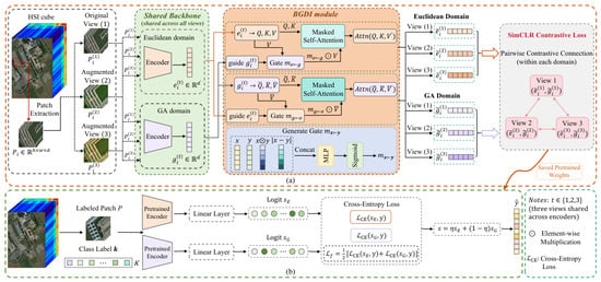
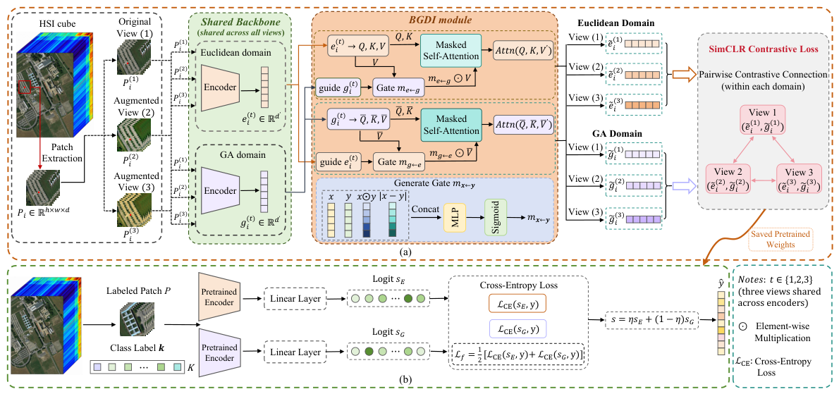
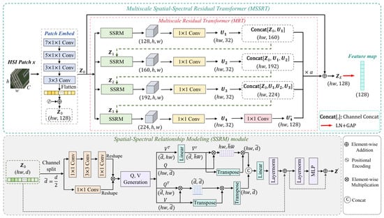
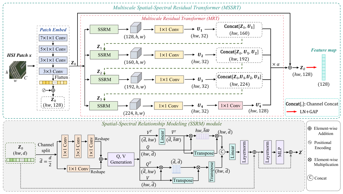


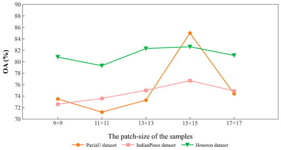
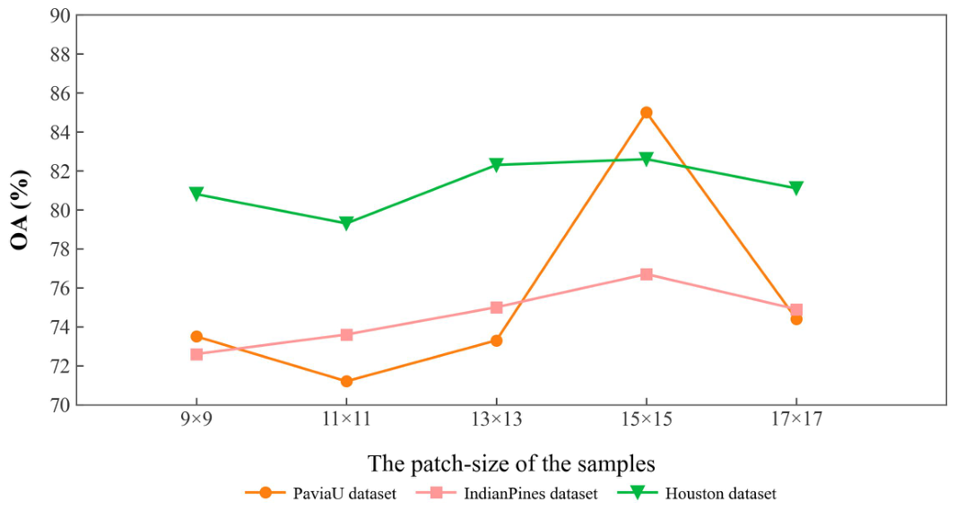
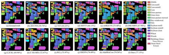
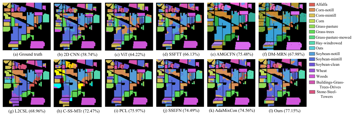
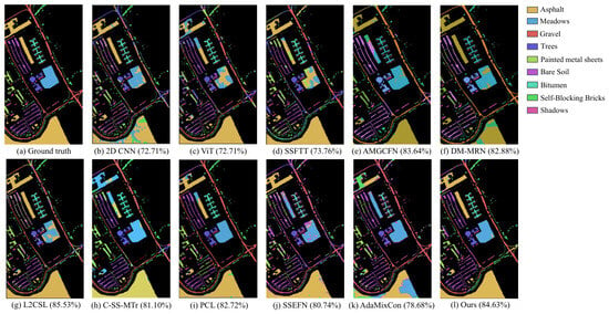
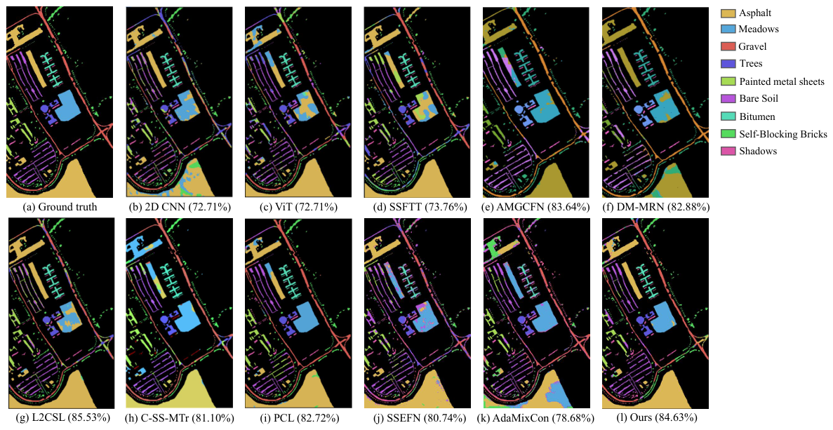
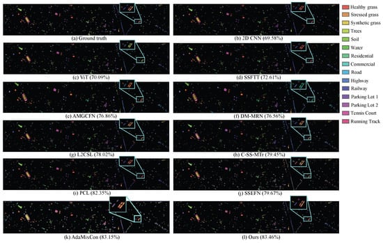
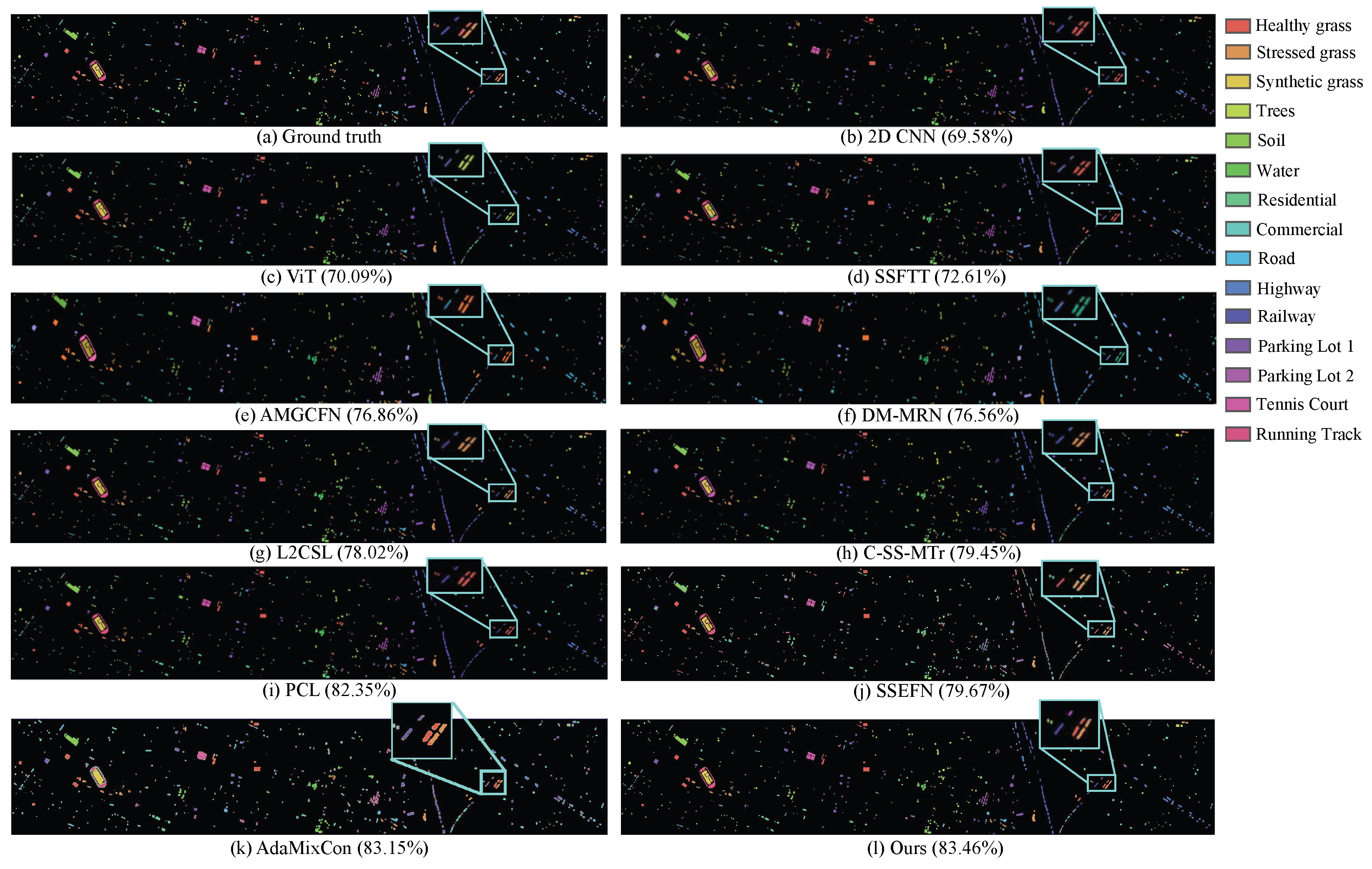
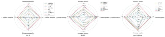
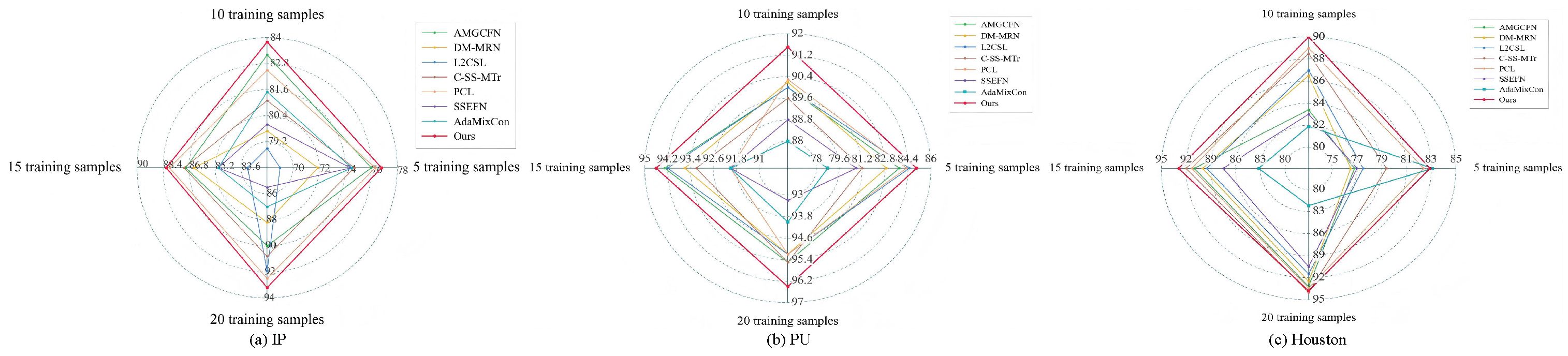

Disclaimer/Publisher’s Note: The statements, opinions and data contained in all publications are solely those of the individual author(s) and contributor(s) and not of MDPI and/or the editor(s). MDPI and/or the editor(s) disclaim responsibility for any injury to people or property resulting from any ideas, methods, instructions or products referred to in the content. |
© 2026 by the authors. Licensee MDPI, Basel, Switzerland. This article is an open access article distributed under the terms and conditions of the Creative Commons Attribution (CC BY) license.