Applicability Evaluation of BRDF Inversion Models at High-Resolution Scale Based on UAV Multiangle Multispectral Images

Highlights

What are the main findings?

• For the ten types of natural and artificial ground targets collected in this study, all five BRDF models are applicable at UAV high-resolution scales when using all observation data.
• Model performance depends on observation planes: RTLSR_C excels with cross principal plane data, ERPV with principal plane data, and HSH with full-plane data, but the performance of the HSH is limited by the number of observations.

What are the implications of the main findings?

• Provides a quantitative basis for selecting appropriate BRDF models for high-resolution multiangle UAV applications under different data availability.
• Reveals that the green camouflage net exhibits multispectral–angular characteristics similar to natural grassland, supporting camouflage target detection and classification.

Abstract

With the development of uncrewed aerial vehicle (UAV) multiangle and multispectral observation, whether bi-directional reflectance distribution function (BRDF) models are applicable to high spatial resolution has become the focus of researchers. However, previous studies usually focus on soil-vegetation BRDF models, limited to certain natural types. In this study, UAV multispectral and multiangle observations were conducted over both natural and artificial targets, to investigate the heterogeneity and similarity among different targets. Five representative BRDF models were selected for inversion, including the Walthall model, the seven-parameter model with double-peak, the RossThick-LiSparseReciprocal-Chen (RTLSR_C) kernel-driven model, the Enhanced Rahman–Pinty–Verstraete (ERPV) model, and the Hemisphere Harmonics (HSH) basis model. To compare the ability of these models in capturing the optical scattering characteristics, observation data from different observation planes were used for fitting. The results show that: (1) The five selected BRDF models generally remain applicable at the UAV scale based on the fitting RMSEs. (2) When only the cross principal plane (CPP) data are used, the RTLSR_C model achieves the best inversion performance. When only the principal plane (PP) data are used, the ERPV model performs best. (3) The multispectral characteristics of the green camouflage net are most similar to that of the grassland.

1. Introduction

The natural surface types of the earth exhibit obvious reflectance anisotropy. Under the same solar zenith angle (SZA) and solar azimuth angle (SAA), the observed reflectance of surface targets varies with the viewing direction [1]. The directional reflectance characteristic of the surface target is described by the bi-directional reflectance distribution function (BRDF) [2]. After extensive research, BRDF models are mainly divided into physical models, empirical models, and semi-empirical models.

Physical models primarily include geometric-optical models, radiative transfer models [3], hybrid models, and computer-simulation models [4]. Empirical models fit sufficient bi-directional reflectance observation data using empirical formulas, providing statistical descriptions or correlations of the measured data. Representative models include the Minnaert model [5] and subsequent developments based on it, such as the Hapke, Veverka, and Wasserman models [6,7,8], as well as the Walthall model [9]. Semi-empirical models are physically informed empirical models that retain key physical principles while maintaining the simplicity of statistical formulations, enabling rapid inversion of spatial BRDF characteristics. Representative models include the seven-parameter model [10], kernel-driven models [11], and the Rahman-Pinty-Verstraete (RPV) model [12]. Considering that some targets exhibit bi-modal reflectance characteristics, the double-peak seven-parameter model was proposed [13]. The Enhanced Rahman-Pinty-Verstraete (ERPV) model introduces a hotspot-related exponential function into the RPV model to account for the hotspot effect with more detail [14]. Building on existing hotspot functions used in the kernel-driven model, Jiao et al. proposed a hotspot-corrected RossThick-Chen (RTC, KRTC) volumetric scattering kernel [15]. Similar to volumetric hotspot corrections, Dong et al. proposed a corrected geometric-optical kernel, KLSRC [16]. The combination of KRTC and KLSRC is referred to as the RossThickLiSparseReciprocal-Chen (RTLSR_C) kernel-driven model. In addition, Qin et al. proposed a general approach based on Hemisphere Harmonics (HSH) basis functions, using mathematical approximation to fit spatial BRDF [17]. Validation on satellite datasets covering 16 land-cover types and uncrewed aerial vehicle (UAV) datasets covering six types demonstrated that this method achieves high accuracy and generality.

BRDF inversion requires multiangle observation data, which are typically obtained from satellite, airborne, or ground-based measurements. In the past decade, UAVs have been able to carry various sensors, either remote control or along preplanned flight paths, to acquire BRDF information of the same surface target from multiple viewing directions in three-dimensional space. UAV offers advantages such as low cost, high spatial resolution, high efficiency, and operational repeatability [18,19]. Many BRDF models derived from satellite images demonstrate high accuracy in fitting quality, BRDF shape, and reflectance errors at the UAV scale [18]. By using four Lambertian reference panels with different reflectance as targets, combined with UAV multispectral multiangle hemispherical observations and spectroradiometer measurements, the potential of UAV multispectral data for BRDF calibration had been confirmed [20]. Moreover, researchers had applied two semi-empirical BRDF models (i.e., RPV and RTLSR) to determine the optimal minimum pixel scale at the UAV scale [21]. Cao et al. employed the Walthall, RPV, and RTLSR models to construct spatial BRDF at UAV scale for four types of ground targets (i.e., Lambertian reference panels, tree canopies, soil, and grass) [22]. Building on this, for grass, bare soil, and wheat, six resampled high-resolution (0.25–8 m) multiangle datasets were used to compare the scale-awareness of various kernel combinations in kernel-driven models and RPV models [23]. Beyond evaluating the applicability of BRDF models under high-resolution conditions, BRDF information contained in UAV multiangle images has shown potential applications in several fields. Combining UAV multiangle hyperspectral observations and BRDF parameters with digital orthophoto maps can significantly improve fine-scale vegetation classification accuracy [24]. Liu et al. explored the integration of multiangle data, deep learning, and scene analysis, incorporating BRDF parameters for target image analysis [25,26]. In addition, the BRDF characteristics of artificial surfaces were investigated, such as asphalt pavements [27], urban scenes [28], and camouflage fabrics and nets [29].

Although previous studies have utilized UAV multispectral multiangle data to explore the applicability of different BRDF models at high spatial resolution, the ground target types considered are limited. Notably, most studies have focused primarily on certain natural surface types, lacking an analysis of spectral-angular reflectance characteristics for a wide range of target types. In addition, a representative set of BRDF models has not been systematically compared in terms of their inversion and reconstruction capabilities. Moreover, the performance of different BRDF models in reconstructing spatial reflectance under incomplete plane datasets remains insufficiently explored.

Based on the previous study [30], this study compares the fitting accuracy of five representative BRDF models at high spatial resolution scales, focusing on evaluating their ability to infer global angle spatial reflectance under limited observation data conditions. Section 2 introduces the multispectral multiangle data of ten types of ground targets, as well as the five representative BRDF models. Section 3 presents the inversion results of different BRDF models, including the comparison of the accuracy in reconstructing BRDF based on different observation plane datasets. Section 4 and Section 5 provide a discussion and conclusion of the research findings.

2. Materials and Methods

2.1. Data and Areas

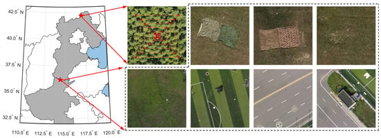
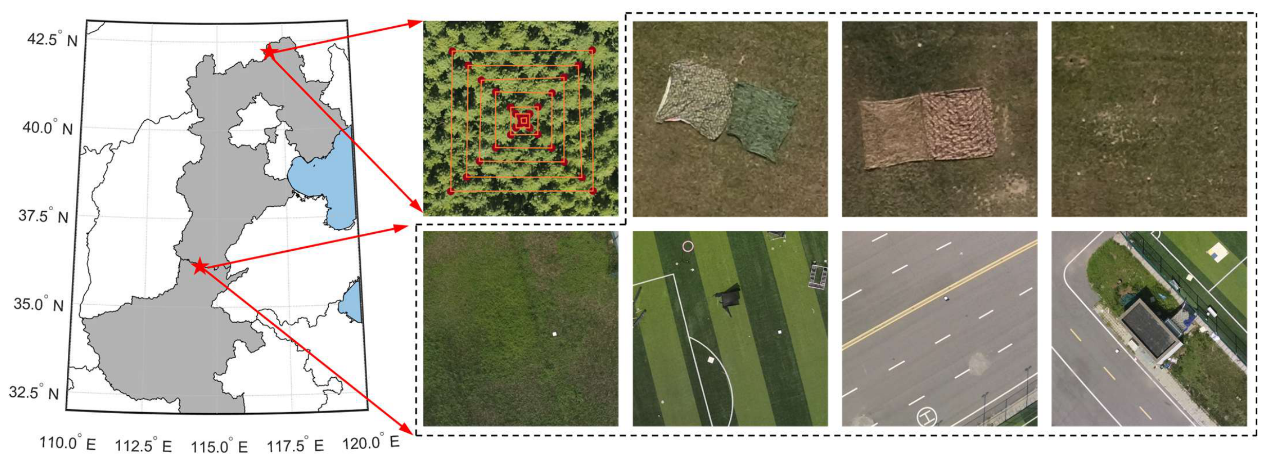
The data used in this study were partly acquired from the larch forest in the Saihanba National Forest Park, located in Chengde City, Hebei Province, within Saihanba National Nature Reserve (42°19′N–42°32′N, 116°53′E–117°32′E). Elevations range from 1010 to 1940 m. The high spatial resolution data were collected on 29 July 2022 at a flight altitude of 200 m. The remaining data were collected at the UAV Flight Center in Beiguan District, Anyang City, Henan Province (36°08′55.61″N, 114°23′20.15″E). The acquisition dates were 13–14 August 2023 at a flight altitude of 50 m and 2–3 December 2024 at a flight altitude of 100 m. The UAV high spatial resolution dataset includes larch forest, natural turf from different periods, artificial turf, asphalt road, cement hut, and four types of camouflage fabrics and nets with different colors and materials. These ground targets exhibit a range of three-dimensional geometric structures from homogeneous to complex, covering both natural and artificial categories. The size of the cement hut is 6.2 m × 3.3 m × 4.5 m, while the camouflage fabrics and nets measure 6 m × 6 m. Figure 1 shows the study area, with the left side illustrating the geographic extent and the right side presenting various ground target types. All target high-resolution images were captured with a view zenith angle (VZA) of 0°.

Figure 1. Sites and schematic illustrations of ground target types in the study area. The red stars indicate the two data observation sites, located in Hebei Province and Henan Province, respectively. The ground target types from the top left to the bottom right are larch forest, green camouflage fabric and net, yellow camouflage fabric and net, grassland, natural turf, artificial turf, asphalt road and cement hut, respectively.

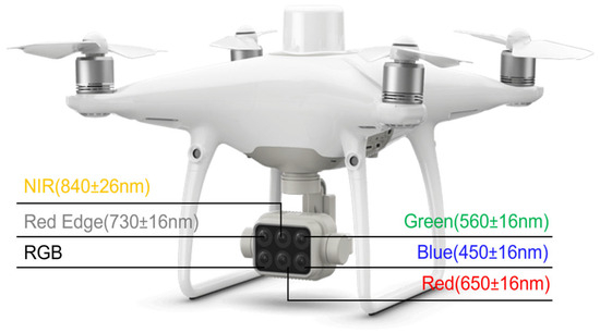
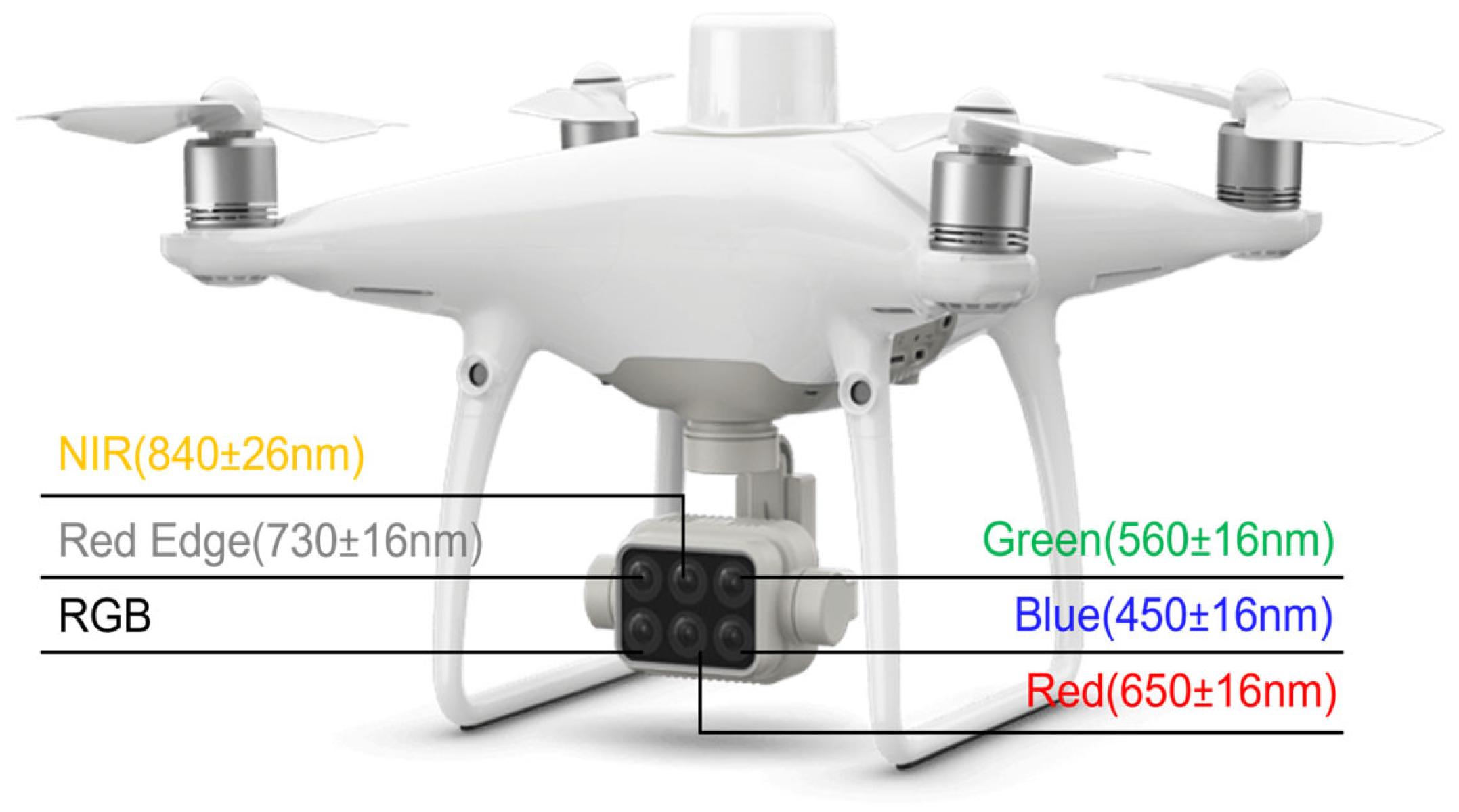
Multispectral multiangle data were acquired by the DJI P4 Multispectral (P4M) measurement system. The DJI P4M integrates an aircraft, gimbal, RTK module, and multispectral camera. It employs an onboard D-RTK system and Ocusync high-definition image transmission. This system is equipped with a two-megapixel visible-light camera and a multispectral camera with five bands (i.e., blue, green, red, red edge, and near-infrared). The corresponding band parameters are shown in Figure 2. The ground sampling distance (GSD) of the DJI P4M is calculated as the flight altitude (H) divided by 18.9 cm per pixel, i.e., GSD = H/18.9 cm/pixel.

Figure 2. DJI P4M UAV remote sensing measurement system.

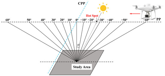
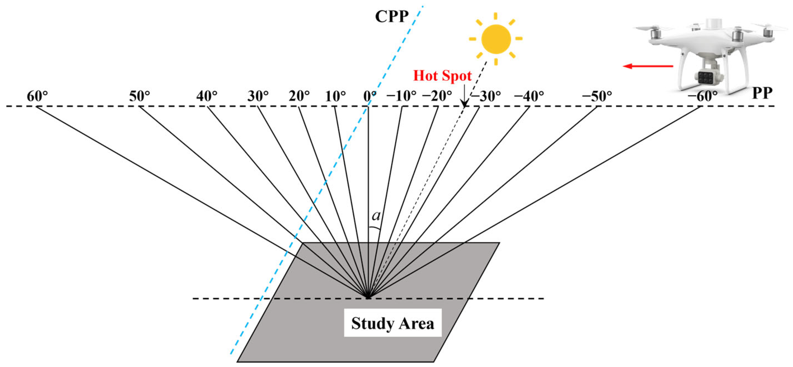
The UAV high-resolution multispectral data were acquired using a linear multiangle observation mode. In this mode, the UAV is oriented toward the center of the study area at different waypoints and flies along a horizontal flight path at a specified altitude. Observations were conducted on the principal plane (PP) and cross principal plane (CPP). The VZA ranged from −60° (backward) to +60° (forward) at 10° intervals. Additionally, based on the local SZA at the time of observation, extra measurements were taken to capture hotspot effects (see Figure 3). Details of the observation data for the ten ground target types are listed in Table 1, in which the other three angles are given, including SZA, SAA, and view azimuth angle (VAA) in the PP and CPP.

Figure 3. The UAV multiangle observation mode varying with VZA (i.e., a).

Table 1. Information of the UAV flight experiments.

Ground Target	Date	Flight Time	GSD (cm/Pixel)	VAA in the PP/CPP (deg)	SAA (deg)	SZA (deg)
Green Camouflage Fabric and Net	3 December 2024	11:00–11:05	5.29	160/250	160	61
		11:10–11:15
Yellow Camouflage Fabric and Net	4 December 2024	12:30–12:35	5.29	176/266	184	58
		12:40–12:45
Grassland	3 December 2024	12:00–12:05	5.29	184/274	176	58
		12:10–12:15
Larch Forest	29 July 2022	15:08–15:15	10.58	248/338	248	42
		15:17–15:23
Natural Turf	13 August 2023	9:31–9:35	2.65	106/196	106	45
		9:50–9:53
Artificial Turf	14 August 2023	9:34–9:37	2.65	106/196	106	45
		9:50–9:53
Asphalt Road	13 August 2023	10:32–10:35	2.65	121/211	121	34
		10:49–10:52
Cement Hut	14 August 2023	10:59–11:03	2.65	132/212	132	29
		11:19–11:22

2.2. Multispectral High-Resolution Image Preprocessing for BRF Extraction

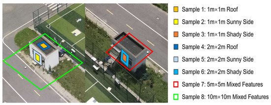
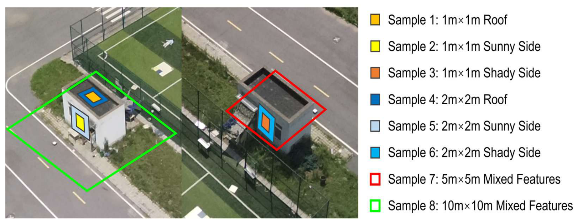
The three-dimensional reconstruction of different ground target scenes was constructed through Agisoft Metashape PhotoScan Pro v1.8.5. According to the characteristics and dimensions of the ground targets, appropriate plot scales were designed. In the orthographic view of the reconstructed scenes, square plots of different scales were manually marked in the central study area. For the larch forest, square plots with scales of 2 m, 5 m, 10 m, 20 m, 30 m, 40 m, 50 m, and 100 m were selected (see Figure 1). For natural turf, artificial turf, and asphalt roads, square plots with scales of 1 m, 2 m, 5 m, 10 m, and 20 m were used. For the cement hut, square plots with scales of 1 m, 2 m, 5 m, and 10 m were chosen. Since the cement hut is a fine-scale three-dimensional structure, for the scales of 1 m and 2 m, separate plots were marked for the roof, sunny sides, and shady sides. When the scale was expanded to 5 m, it included surrounding background areas, forming mixed target types. The marking procedure is shown in Figure 4. For grassland and camouflage fabrics and nets of different colors and materials, square plots with scales of 1 m, 2 m, and 5 m were selected.

Figure 4. Distribution of cement hut marking areas.

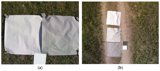
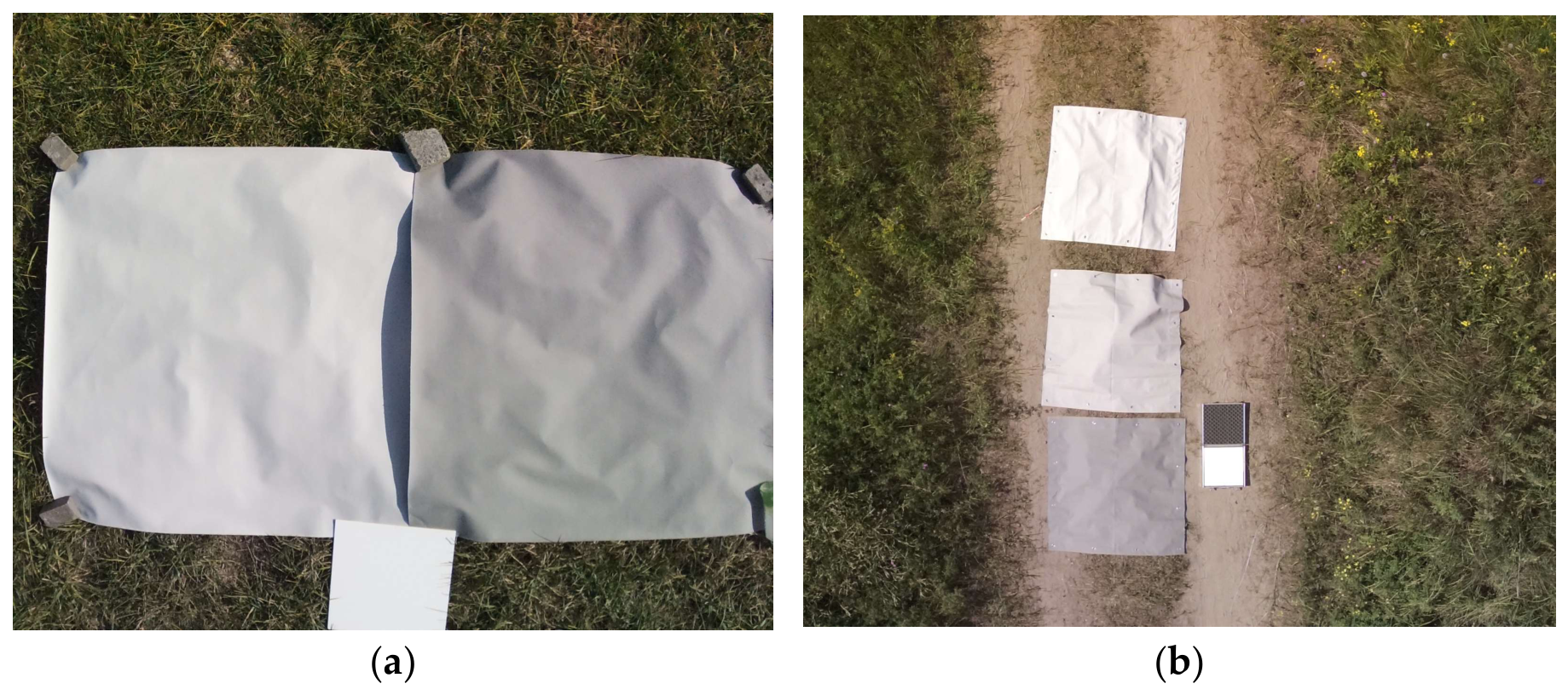
The raw UAV multispectral multiangle data are gray value matrices without physical meaning. The raw UAV multispectral multiangle data were preprocessed. Exposure, vignetting, and illumination corrections were completed by retrieving the parameter information from the P4M multispectral system. Radiometric calibration was performed using Lambertian reflectance panels, converting gray value matrices into the bi-directional reflectance factor (BRF). The coefficients a and b of a linear regression function were derived from the mean digital number (DN) values of one or multiple Lambertian reflectance panels and their corresponding reflectance. The least squares method was selected for parameter fitting. After radiometric calibration performed via (1), the BRF of each pixel in the UAV high-resolution multispectral images can be obtained [31]. During the 2022 observation in the larch forest of Saihanba, four Lambertian reflectance panels with BRFs of 20%, 40%, 60%, and 95% were placed near the study area. In the 2023 observation at the UAV Flight Center in Anyang, one Lambertian reflectance panel with 95% BRF was placed near the study area (b was set to 0 for fitting). For the 2024 observation, three Lambertian reflectance panels with BRFs of 20%, 60%, and 95% were positioned near the study area. The placements of the Lambertian reflectance panels are shown in Figure 5.

$$\mathrm{BRF}=a\cdot \mathrm{DN}+b$$

(1)

Figure 5. Schematic illustration of Lambertian reference panels. (a) shows those used in the 2024 observation. (b) shows those used in the 2022 observation.

2.3. BRDF Reconstruction Based on Five Representative BRDF Models

2.3.1. Walthall Model

The Walthall model is an empirical model that describes the functional relationship between reflectance and the VZA, VAA, and SAA [9]. By integrating over the hemisphere, the functional relationship between hemispherical reflectance and the coefficients of a simple equation is obtained.

$$R({\theta }_v,{\phi }_v)=a{\theta }_v^2+b{\theta }_v\cos ({\phi }_v-{\phi }_s)+c$$

(2)

where R is the reflectance, θ_v is the VZA, φ_v is the VAA, and φ_s is the SAA. The coefficients a, b, and c are obtained through linear least-squares fitting.

2.3.2. Seven-Parameter with Double-Peak Model

Considering the diversity of ground target types, the seven-parameter model capable of fitting both unimodal and bimodal characteristics was selected [13]. The model consists of specular and diffuse reflection components. The specular component incorporates two exponential terms, enabling a more accurate description of target reflectance under multiple illumination angles.

$$R({\theta }_s,{\theta }_v,{\phi }_v)=k_a\exp \left[k_1{\left(1-\cos {\gamma }_1\right)}^a\right]+k_b\exp \left[k_2{\left(1-\cos {\gamma }_2\right)}^b\right]+{\displaystyle \frac{k_c}{\cos {\theta }_s}}$$

(3)

where

$$\begin{array}{l}\cos {\gamma }_1={\displaystyle \frac{\cos {\theta }_s\cos {\theta }_v-\sin {\theta }_s\sin {\theta }_v\cos ({\phi }_v-{\phi }_s)+1}{2}}\\ \cos {\gamma }_2={\displaystyle \frac{\cos {\theta }_s\cos {\theta }_v+\sin {\theta }_s\sin {\theta }_v\cos ({\phi }_v-{\phi }_s)+1}{2}}\end{array}$$

(4)

In Equation (3), k_a and k_b are the specular reflection coefficients, and k_c is the diffuse reflection coefficient. The parameters k₁, k₂, a and b control the shape of the reflectance peaks. The intermediate variables γ₁ and γ₂ describe the angular relationships between the incident and reflected directions, corresponding to the two reflection peaks, respectively. In Equation (4), θ_s is the SZA, and φ_s is the SAA. θ_v and φ_v represent the VZA and VAA.

2.3.3. RossThickLiSparseReciprocal-Chen (RTLSR_C) Kernel-Driven Model

The RTLSR_C model represents bi-directional reflectance as a linear combination of three scattering components: isotropic scattering, volumetric scattering, and geometric optical scattering, and each scattering is associated with its corresponding kernel. The model formulation is given in Equation (5).

$$R\left({\theta }_s,{\theta }_v,\phi ,\lambda \right)=f_{iso}\left(\lambda \right)+f_{vol}\left(\lambda \right)K_{vol}\left({\theta }_s,{\theta }_v,\phi \right)+f_{geo}\left(\lambda \right)K_{geo}\left({\theta }_s,{\theta }_v,\phi \right)$$

(5)

where R(θ_s, θ_v, φ, λ) refers to the BRDF in the band λ, and K_vol(θ_s, θ_v, φ) and K_geo(θ_s, θ_v, φ) are the volume scattering kernel and geometric-optical scattering kernel, respectively. Both of them are functions of the incident SZA θ_s, the VZA θ_v, and the relative azimuth angle (RAA) φ.

The RTLSR_C model was selected in this study, which incorporates the hotspot-corrected volume scattering kernel Rossthick-Chen (RTC) K_RTC and geometric-optical scattering kernel LiSparseReciprocal-Chen (LSRC) K_LSRC [15,16].

$$K_{\mathrm{RTC}}={\displaystyle \frac{\left(\pi /2-\xi \right)\cos \xi +\sin \xi }{\cos {\theta }_v+\cos {\theta }_s}}\times \left(1+C_1{e}^{-\xi /C_2}\right)-{\displaystyle \frac{\pi }{2}}$$

(6)

$$K_{\mathrm{LSRC}}=O\left({\theta }_s^{\prime },{\theta }_v^{\prime },t\right)\left(1+C_1{e}^{-\xi /C_2}\right)-\sec {\theta }_s^{\prime }-\sec {\theta }_v^{\prime }+{\displaystyle \frac{1}{2}}\left(1+\cos {\xi }^{\prime }\right)\sec {\theta }_v^{\prime }\sec {\theta }_s^{\prime }$$

(7)

where ξ is the phase angle between the directions of incidence and observation. The expression 1 + C₁e^−ξ/C2 is the hotspot function, which encompasses two undetermined parameters of C₁ and C₂ indicating the height and width of the hotspot reflectance, respectively [16]. The RTLSR_C model was originally developed primarily for continental vegetation canopies and soils. However, based on our previous analysis of the 3D structural characteristics of artificial targets, the volumetric scattering kernel of the model remains applicable to solid materials and those with purely specular/diffuse reflectance [30].

2.3.4. Enhanced Rahman-Pinty-Verstraete (ERPV) Model

The RPV model is an early semi-empirical bi-directional reflectance model that approximates the BRF of any surface based on the geometry of illumination and observation. The ERPV model extends the RPV model by introducing the exponential hotspot function into the hotspot term [14], leading to a more accurate depiction of the height and width of the hotspot.

$$R({\theta }_s,{\theta }_v,{\phi }_s,{\phi }_v)={\rho }_0\times M({\theta }_s,{\theta }_v,k)\times F(g)\times \left[1+{\displaystyle \frac{1-{\rho }_0}{1+G}}\times \left(1+C_1\exp \left(-{\displaystyle \frac{\xi }{C_2}}\right)\right)\right]$$

(8)

$$M({\theta }_s,{\theta }_v,k)={(\cos {\theta }_s\cos {\theta }_v)}^{k-1}{(\cos {\theta }_s+\cos {\theta }_v)}^{k-1}$$

(9)

$$F(g)={\displaystyle \frac{1-{\Theta }^2}{{[1+{\Theta }^2+2\Theta \cos g]}^{1.5}}}\hspace{1em}$$

(10)

$$\cos g=\cos {\theta }_s\cos {\theta }_v+\sin {\theta }_s\sin {\theta }_v\cos ({\phi }_s-{\phi }_v)$$

(11)

$$[1+R(G)]=1+{\displaystyle \frac{1-{\rho }_c}{1+G}}$$

(12)

$$G=\sqrt{{\tan }^2{\theta }_s+{\tan }^2{\theta }_v-2\tan {\theta }_s\tan {\theta }_v\cos ({\phi }_s-{\phi }_v)}$$

(13)

$$\xi ={\cos }^{-1}[\cos {\theta }_s\cos {\theta }_v+\sin {\theta }_s\sin {\theta }_v\cos ({\phi }_s-{\phi }_v)]$$

(14)

where M(θ_s, θ_v, k) is the modified Minnaert function. F(g) is the Henyey-Greenstein phase function, and [1 + R(G)] is the original hotspot term. ξ is the phase angle between the directions of incidence and observation. There are two undetermined parameters of C₁ and C₂ indicating the height and width of the hotspot reflectance, respectively [14]. θ_s and φ_s represent the SZA and SAA. θ_v and φ_v represent the VZA and VAA.

2.3.5. Hemisphere Harmonics (HSH) Basis Model

Existing empirical or semi-empirical BRDF models are often limited to specific land cover types because they rely on assumptions about the distribution of surface depressions. To overcome the restriction of these models to particular surface types, high-precision BRDF representation can be achieved by deriving HSH basis functions that match the BRDF domain, expressed as an infinite series. The HSH basis functions are complete and orthogonal, enabling the approximation of any BRDF dataset [17].

$$R(\theta ,\phi )\approx {\displaystyle \sum _{l=0}^n{\displaystyle \sum _{m=-l}^l{c}_l^m}}{H}_l^m(\theta ,\phi )$$

(15)

$$c_l^m={\displaystyle {\int }_0^{2\pi }{\displaystyle {\int }_0^{\pi /2}R}}(\theta ,\phi )H_l^m(\theta ,\phi )\sin \theta d\theta d\phi$$

(16)

$$H_l^m(\theta ,\phi )={\tilde{N}}_l^m{\tilde{P}}_l^m(\cos \theta )e^{im\phi }$$

(17)

$${\tilde{N}}_l^m=\sqrt{{\displaystyle \frac{2l+1}{2\pi }}\cdot {\displaystyle \frac{(l-|m|)!}{(l+|m|)!}}}$$

(18)

$${\tilde{P}}_l^m(\cos \theta )=P_l^m(2\cos \theta -1),\hspace{1em}\theta \in [0,\pi /2]$$

(19)

where θ is the VZA, and φ is the relative azimuth angle. The coefficient c_l^m is calculated via inner products. H_l^m(θ, φ) represents the HSH basis functions. Ñ_l^m is the normalization factor. ${\tilde{P}}_l^m(\cos \theta )$ denotes the shifted associated Legendre polynomials. When discrete observation data are used, the linear system is solved by the least squares method. To uniquely solve the system of linear equations, the number of observations M must be no less than the square of the order n + 1.

2.4. Evaluation Metrics

2.4.1. Quantitative Evaluation Metrics for BRDF Models

To quantitatively evaluate the performance of different BRDF models, the degrees-of-freedom-adjusted root mean square error (RMSE) and Pearson correlation coefficient (PCC) were used. The RMSE was adjusted for degrees of freedom to prevent overestimation of fitting accuracy due to differences in the number of model parameters. The degrees-of-freedom-adjusted RMSE is calculated as follows:

$$RMSE=\sqrt{{\displaystyle \frac{{\displaystyle {\sum }_{i=1}^n{(\rho -{\rho }^{\prime })}^2}}{n-p}}}$$

(20)

where ρ represents the UAV-observed BRF, ρ′ represents the model inversion BRF, n is the number of observation data points, and p is the number of model parameters. The Walthall model has three parameters, the seven-parameter with double-peak model has seven parameters, the RTLSR_C model has three parameters, the ERPV model has five parameters, and the HSH model has a parameter count corresponding to its order. Based on statistics calculated from vegetation and bare soil reported in [32], the expected RMSEs for different spectral bands are summarized in Table 2. The range is used as the benchmark for assessing the inversion performance of the five representative BRDF models.

Table 2. Requirement of RMSE values across different bands.

Band	RMSE
Blue	≤0.01
Green	≤0.04
Red	≤0.02
Red Edge	≤0.05
Near-Infrared	≤0.05

In addition to the RMSE, the PCC was introduced to quantitatively evaluate the consistency between the observed and model-reconstructed angular BRF patterns. The PCC ranges from −1 to 1, with values closer to 1 indicating greater consistency in the angular variation pattern. RMSE therefore characterizes the magnitude of reconstruction errors, whereas PCC provides a complementary measure of angular-pattern similarity.

$$\mathrm{PCC}={\displaystyle \frac{{\displaystyle \sum _{i=1}^n\left({\rho }_i-\overline{\rho }\right)}\left({\rho }_{i^{\prime }}-{\overline{\rho }}^{\prime }\right)}{\sqrt{{\displaystyle \sum _{i=1}^n{\left({\rho }_i-\overline{\rho }\right)}^2}}\sqrt{{\displaystyle \sum _{i=1}^n{\left({\rho }_{i^{\prime }}-{\overline{\rho }}^{\prime }\right)}^2}}}}$$

(21)

where ρ_i represents the UAV-observed BRF at the i viewing direction, and ρ_i′ represents the BRF reconstructed by the BRDF model at the corresponding viewing direction. $\overline{\rho }$ and ${\overline{\rho }}^{\prime }$ denote the mean observed and model-reconstructed BRFs over all viewing directions, respectively. n is the number of observations.

2.4.2. Spectral Similarity Metrics Based on the Grassland Background

To quantitatively evaluate the spectral similarity between the camouflage fabric and net of different colors and the grassland background, the Spectral Angle Mapper (SAM) and the corresponding root mean square error (RMSE_SAM) were employed. The spectral similarity between the camouflage target and the grassland background was evaluated in terms of both spectral shape and reflectance value. SAM measures the similarity in spectral shape by calculating the angle between two spectral vectors in a multidimensional spectral space. A smaller SAM value indicates a higher similarity in spectral shape between the camouflage target and the grassland background. For the j observation direction, SAM is defined as

$${\theta }_{\mathrm{SAM},j}=\arccos \left({\displaystyle \frac{{\displaystyle \sum _{i=1}^n{R}_{t,j,i}}{R}_{b,j,i}}{\sqrt{{\displaystyle \sum _{i=1}^n{R}_{t,j,i}^2}}\sqrt{{\displaystyle \sum _{i=1}^n{R}_{b,j,i}^2}}}}\right)$$

(22)

where R_t,j,i and R_b,j,i represent the reflectance of a given type of camouflage fabric or camouflage net and the grassland background, respectively, in the i spectral band under the j observation direction.

RMSE_SAM characterizes the average deviation in reflectance between the target and background across the spectral bands. A smaller RMSE_SAM indicates a smaller difference in absolute reflectance and a higher similarity in spectral value between the target and background. The RMSE_SAM corresponding to the SAM calculation for the j observation direction is calculated as follows, where i denotes the five spectral bands. A smaller RMSE_SAM indicates that the reflectance values of the camouflage fabric and net are more similar to those of the grassland background.

$${\mathrm{RMSE}}_{\mathrm{SAM},j}=\sqrt{{\displaystyle \frac{1}{n}}{\displaystyle \sum _{i=1}^n{\left(R_{t,j,i}-R_{b,j,i}\right)}^2}}$$

(23)

3. Results

3.1. Comparison of BRDF Model Inversion Based on Various Ground Targets

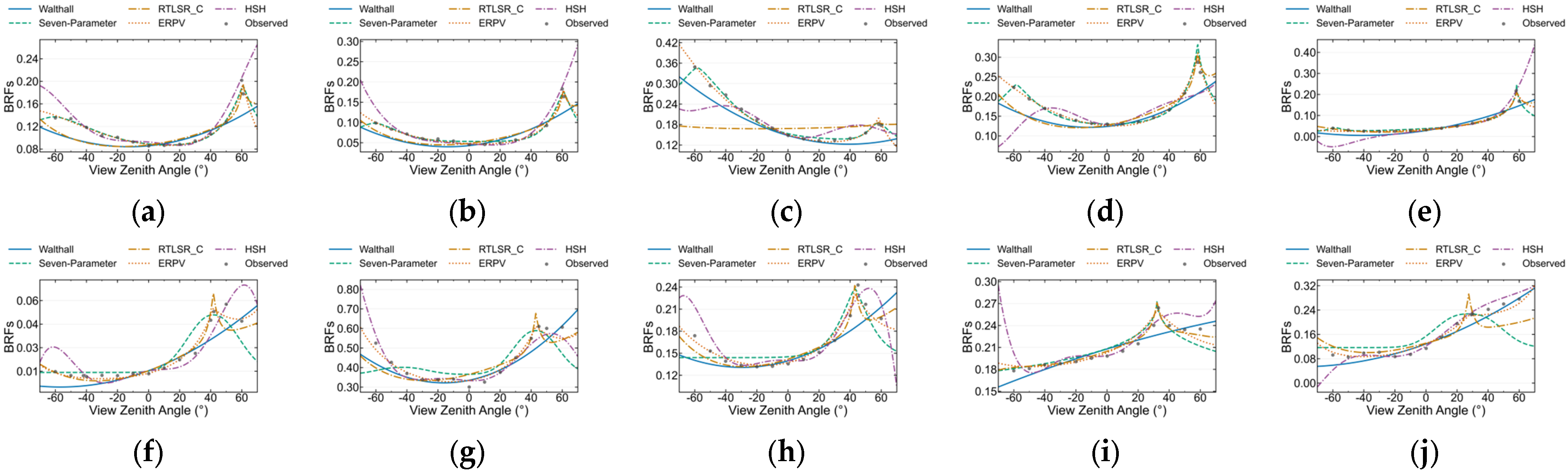
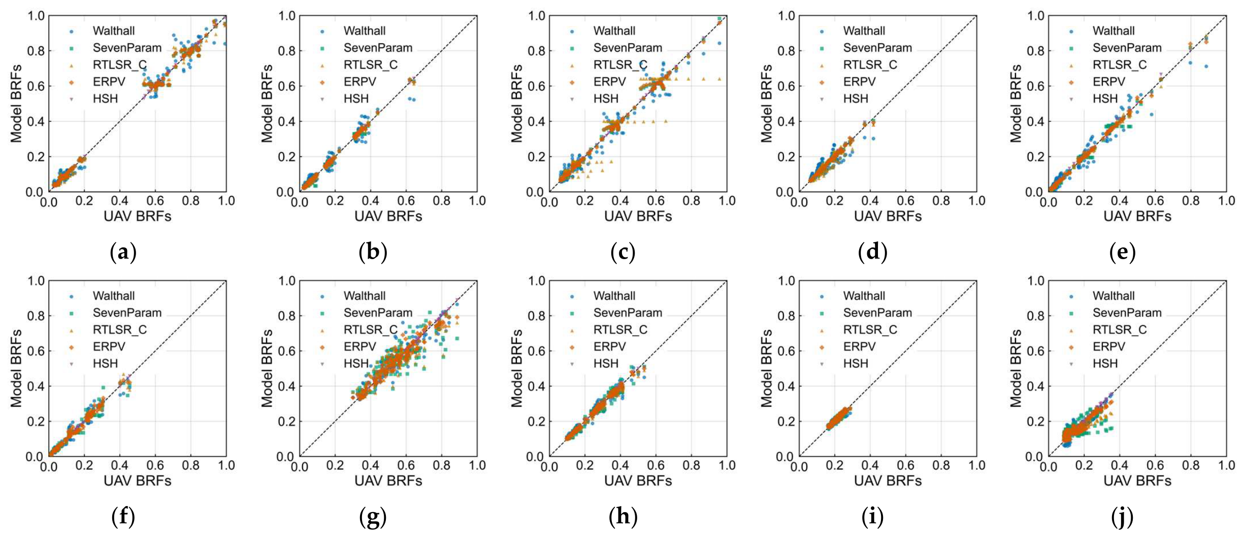
Based on the model formulations, all observation data for each ground target type were input into the five BRDF model expressions to estimate parameters and reconstruct BRDF. In the representative red band, the inversion performance of the five BRDF models was compared under the 5 m scale. Figure 6 presents the BRDF inversion results in the PP. To further quantify the inversion capability of the five BRDF models, the scatter plots in Figure 7 present comparisons between UAV-observed BRFs and model-inverted BRFs across all spectral bands (i.e., blue, green, red, red edge and near-infrared). For the spectral band, the mean RMSE across all bands was calculated. Table 3 summarizes the RMSEs for the ten target types under the 5 m scale, including results for individual bands and their averages. As the results at other plot scales exhibit similar patterns, only the results at the 5 m scale are presented in this part.

Figure 6. Comparison of BRDF model inversions in the PP for ten ground target types at the 5 m scale in the red band. (a–j) represent green camouflage fabric, green camouflage net, yellow camouflage fabric, yellow camouflage net, grassland, larch forest, natural turf, artificial turf, asphalt road, and cement hut, respectively.

Figure 7. Scatter plot comparison of UAV-observed BRFs and model-inverted BRFs for ten ground target types at the 5 m scale across all spectral bands. (a–j) represent green camouflage fabric, green camouflage net, yellow camouflage fabric, yellow camouflage net, grassland, larch forest, natural turf, artificial turf, asphalt road, and cement hut, respectively.

Table 3. RMSEs of five BRDF models for ten target types in different spectral bands at 5 m scale. The model corresponding to the bold value has the best inversion performance.

Ground Target Types	Model	Blue	Green	Red	Red Edge	NIR	Mean
Green Camouflage Fabric	Walthall	0.0148	0.0246	0.0266	0.0645	0.0809	0.0472
	SevenParam	0.0069	0.0116	0.0120	0.0384	0.0415	0.0236
	RTLSR_C	0.0113	0.0172	0.0181	0.0381	0.0611	0.0329
	ERPV	0.0014	0.0027	0.0041	0.0095	0.0114	0.0239
	HSH	0.0063	0.0107	0.0116	0.0374	0.0409	0.0049
Green Camouflage Net	Walthall	0.0114	0.0198	0.0227	0.0337	0.0471	0.0283
	SevenParam	0.0193	0.0075	0.0083	0.0115	0.0182	0.0123
	RTLSR_C	0.0062	0.0081	0.0109	0.0114	0.0118	0.0095
	ERPV	0.0025	0.0043	0.0054	0.0064	0.0087	0.0054
	HSH	0.0019	0.0033	0.0031	0.0053	0.0074	0.0032
Yellow Camouflage Fabric	Walthall	0.0239	0.0329	0.0349	0.0566	0.0894	0.0507
	SevenParam	0.0058	0.0082	0.0135	0.0218	0.0353	0.0178
	RTLSR_C	0.0348	0.0494	0.0546	0.0802	0.1303	0.0740
	ERPV	0.0042	0.0066	0.0116	0.0205	0.0338	0.0173
	HSH	0.0017	0.0023	0.0023	0.0041	0.0059	0.0025
Yellow Camouflage Net	Walthall	0.0193	0.0290	0.0354	0.0278	0.0451	0.0310
	SevenParam	0.0043	0.0053	0.0046	0.0052	0.0080	0.0050
	RTLSR_C	0.0149	0.0190	0.0223	0.0166	0.0255	0.0191
	ERPV	0.0022	0.0041	0.0038	0.0052	0.0087	0.0049
	HSH	0.0043	0.0077	0.0080	0.0091	0.0147	0.0065
Grassland	Walthall	0.0127	0.0252	0.0234	0.0450	0.0576	0.0349
	SevenParam	0.0047	0.0093	0.0068	0.0250	0.0440	0.0207
	RTLSR_C	0.0032	0.0049	0.0054	0.0085	0.0146	0.0080
	ERPV	0.0040	0.0073	0.0067	0.0113	0.0135	0.0085
	HSH	0.0043	0.0083	0.0075	0.0135	0.0166	0.0076
Larch Forest	Walthall	0.0066	0.0124	0.0074	0.0322	0.0346	0.0214
	SevenParam	0.0047	0.0079	0.0056	0.0293	0.0361	0.0191
	RTLSR_C	0.0026	0.0064	0.0039	0.0197	0.0245	0.0139
	ERPV	0.0024	0.0057	0.0025	0.0188	0.0177	0.0111
	HSH	0.0012	0.0020	0.0015	0.0045	0.0071	0.0029
Natural Turf	Walthall	0.0635	0.0719	0.0524	0.0453	0.0349	0.0526
	SevenParam	0.0883	0.1019	0.0580	0.0675	0.0657	0.0689
	RTLSR_C	0.0620	0.0776	0.0429	0.0475	0.0482	0.0544
	ERPV	0.0363	0.0468	0.0261	0.0356	0.0332	0.0333
	HSH	0.0141	0.0176	0.0145	0.0219	0.0241	0.0128
Artificial Turf	Walthall	0.0131	0.0250	0.0177	0.0270	0.0269	0.0216
	SevenParam	0.0112	0.0226	0.0137	0.0248	0.0300	0.0192
	RTLSR_C	0.0070	0.0145	0.0093	0.0151	0.0179	0.0128
	ERPV	0.0057	0.0123	0.0070	0.0124	0.0125	0.0096
	HSH	0.0061	0.0109	0.0086	0.0136	0.0156	0.0080
Asphalt Road	Walthall	0.0088	0.0111	0.0115	0.0119	0.0125	0.0107
	SevenParam	0.0094	0.0104	0.0108	0.0118	0.0139	0.0100
	RTLSR_C	0.0055	0.0072	0.0076	0.0083	0.0090	0.0073
	ERPV	0.0073	0.0087	0.0089	0.0096	0.0102	0.0083
	HSH	0.0052	0.0068	0.0082	0.0086	0.0100	0.0054
Cement Hut	Walthall	0.0339	0.0317	0.0253	0.0368	0.0383	0.0320
	SevenParam	0.0623	0.0575	0.0484	0.0648	0.0691	0.0541
	RTLSR_C	0.0392	0.0386	0.0319	0.0404	0.0472	0.0380
	ERPV	0.0305	0.0255	0.0198	0.0311	0.0348	0.0266
	HSH	0.0054	0.0054	0.0068	0.0063	0.0059	0.0042

Figure 6 presents a comparison of the five BRDF models for the principal plane (PP) of ten ground target types. The Walthall model produces curves without hotspot effects, showing a simple monotonically increasing or decreasing trend. The seven-parameter with double-peak model, RTLSR_C model, and ERPV model all account for hotspot effects, capturing peak reflectance near the hotspot angle. Moreover, when the hotspot angle is large (around the SZA of 60°), these three models still effectively fit the abrupt reflectance changes in the hotspot region. The HSH basis produces oscillatory curves, reflecting its approach to fitting spatial reflectance.

The scatter distributions in Figure 7 vary across different ground target types, indicating that each type exhibits distinct BRFs and possesses unique optical scattering characteristics. In Figure 7c, it is evident that for the yellow camouflage fabric, the yellow scatter points fitted by the RTLSR_C model show relatively poor agreement, with correspondingly higher RMSE. Figure 7e,g both depict grassland types, but the specific areas and multiangle observation times differ. The scatter distributions reveal differences in their BRF distributions. Figure 7i shows the BRF scatter distribution for the asphalt road, corresponding to the three-dimensional structural characteristics of roads analyzed in [30]. Due to the flatness, simple three-dimensional structure, and uniform color composition of the road, the BRFs are distributed more closely.

Referring to the content of Figure 7 and Table 3, and considering the RMSE ranges presented in Table 2, when both the cross principal plane (CPP) and PP datasets are used, the five BRDF models generally demonstrate applicability for reconstructing BRDFs of multiple ground target types in high spatial resolution images at the 5 m scale. Only a few RMSEs are relatively large, exceeding the ranges shown in Table 2. In this section, the model inversion performance was evaluated using all observations from both the PP and CPP. With sufficient observation data, the model inversion performance decreased in the following order: the HSH model, the ERPV model, the RTLSR_C model, the seven-parameter with double-peak model, and the Walthall model. The HSH model approximates the spatial BRDF using a mathematical fitting approach that depends on the amount of data. The more data available, the higher the fitting order that can be chosen, resulting in smaller RMSEs. Existing experiments indicate that the accuracy of a third-order HSH approximation can reach around 99% [17]. Nevertheless, as the HSH method is purely mathematical, its capability to reconstruct the spatial BRDF of ground targets still requires further investigation.

3.2. Comparison of BRDF Model Inversion Based on Different Plane Datasets

To more comprehensively investigate the applicability of BRDF models at high spatial resolution, BRDF model inversion was performed using observation data from the CPP, the PP, and both planes combined (CPP + PP). Polar-coordinate reflectance images were used to qualitatively compare the fitting performance of different models. Model parameters were inverted using observation data from different planes. After reconstructing the BRDF characteristics of the ground targets, we calculated the RMSEs and PCCs. Specifically, the UAV observation data from both planes (CPP + PP) and the corresponding viewing angles were input into the models. Then, the model-fitted BRF ρ′ were obtained, together with the observed BRF ρ from both planes, and substituted into Equation (20) to calculate the RMSEs. Meanwhile, the BRFs required for calculating the PCCs in Equation (21) can be obtained. It allows for a quantitative comparison of how effectively each BRDF model utilizes observation data from different planes.

Given the large number of observed ground target types, this part presents representative targets. For natural targets, larch forest was selected, and for artificial targets, the asphalt road was chosen. Figure 8 and Figure 9 show the inversion results using different plane datasets, corresponding to spatial reflectance at the 5 m scale in the red band. Correspondingly, Table 4 summarizes the RMSEs for the five BRDF models in these two representative ground target types. Table 5 concisely presents the scale-averaged PCCs for two representative ground targets. The combined use of RMSE and PCC enables a more comprehensive comparison of the fitting performance of the five models using different plane datasets.

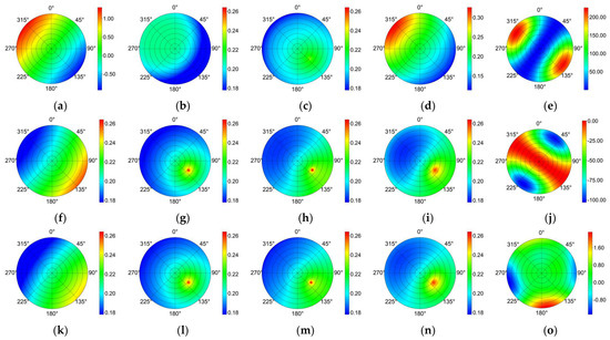
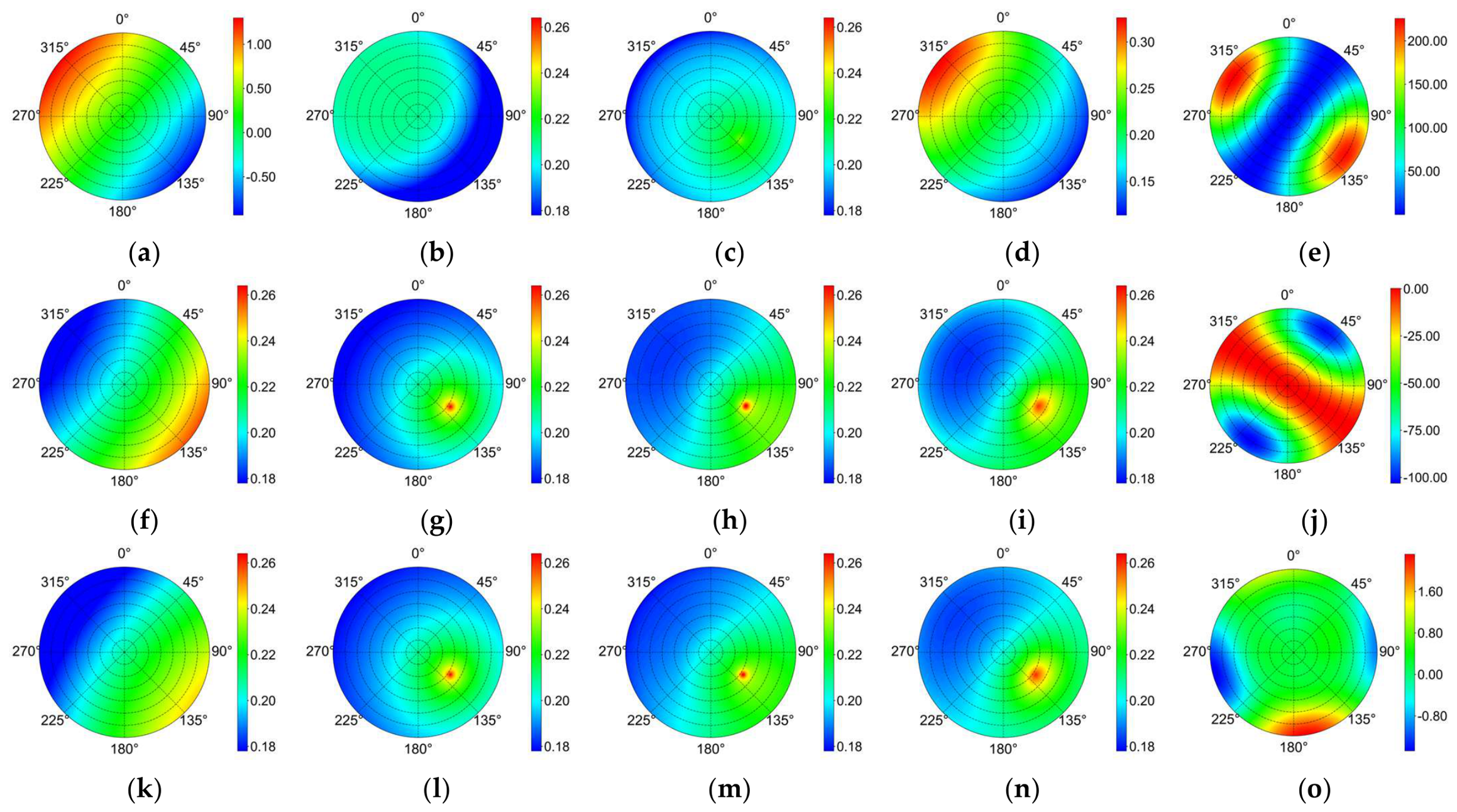
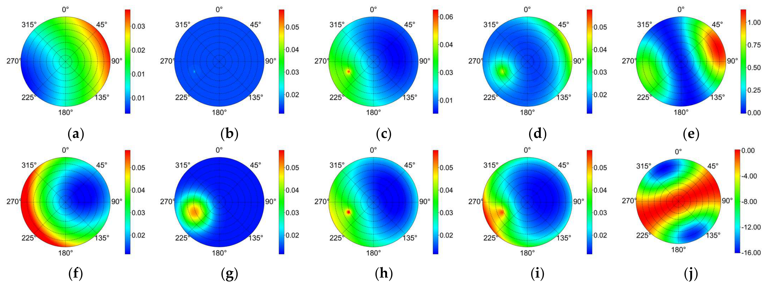
Figure 8. The inversion BRDFs of the five models for larch forest in the red band at the 5 m scale are based on three plane datasets. (a–e) are based on the cross principal plane (CPP) dataset, (f–j) are based on the principal plane (PP) dataset, and (k–o) are based on the CPP + PP dataset. The models in the first to fifth columns are the Walthall model, the seven-parameter with double-peak model, the RTLSR_C model, the ERPV model, and the HSH model.

Figure 9. The inversion BRDFs of the five models for asphalt roads in the red band at the 5 m scale are based on three plane datasets. (a–e) are based on the cross principal plane (CPP) dataset, (f–j) are based on the principal plane (PP) dataset, and (k–o) are based on the CPP + PP dataset. The models in the first to fifth columns are the Walthall model, the seven-parameter with double-peak model, the RTLSR_C model, the ERPV model, and the HSH model.

Table 4. RMSEs of five BRDF model inversions for two representative ground target types at different scales in the red band based on different plane datasets. The model corresponding to the bold value has the best inversion performance.

Ground Target Types	Scale	Plane Dataset	Walthall	SevenParam	RTLSR_C	ERPV	HSH
Larch Forest	2 m	CPP	0.0382	0.0152	0.0136	0.0178	0.2261
		PP	0.0095	0.0086	0.0068	0.0065	3.9850
		CPP + PP	0.0080	0.0082	0.0068	0.0062	0.0022
	5 m	CPP	0.0176	0.0155	0.0041	0.0092	0.5059
		PP	0.0095	0.0060	0.0041	0.0028	8.7381
		CPP + PP	0.0074	0.0056	0.0039	0.0025	0.0015
	10 m	CPP	0.0125	0.0145	0.0059	0.0030	0.0455
		PP	0.0086	0.0046	0.0026	0.0015	9.8019
		CPP + PP	0.0068	0.0042	0.0025	0.0014	0.0012
	20 m	CPP	0.0181	3.1302	0.0037	0.0076	0.0649
		PP	0.0085	0.0034	0.0024	0.0012	9.0430
		CPP + PP	0.0067	0.0031	0.0021	0.0011	0.0011
	30 m	CPP	0.0142	0.0134	0.0054	0.0057	0.0197
		PP	0.0081	0.0035	0.0020	0.0009	9.6753
		CPP + PP	0.0065	0.0032	0.0018	0.0009	0.0011
	40 m	CPP	0.0148	0.1353	0.0034	0.0071	0.0094
		PP	0.0082	0.0033	0.0022	0.0010	9.5297
		CPP + PP	0.0065	0.0030	0.0019	0.0009	0.0011
	50 m	CPP	0.0154	0.0132	0.0021	0.0071	0.1431
		PP	0.0079	0.0035	0.0022	0.0010	8.6685
		CPP + PP	0.0063	0.0032	0.0020	0.0009	0.0010
	100 m	CPP	0.0142	3.0647	0.0020	0.0069	0.0881
		PP	0.0071	0.0122	0.0021	0.0010	6.1526
		CPP + PP	0.0055	0.0030	0.0019	0.0009	0.0007
	Mean	CPP	0.0188	1.3770	0.0059	0.0083	0.1764
		PP	0.0081	0.0057	0.0033	0.0025	7.1828
		CPP + PP	0.0064	0.0040	0.0031	0.0023	0.0009
Asphalt Road	1 m	CPP	4.6933	0.0926	0.0786	0.1312	35.2821
		PP	0.0499	0.0715	0.0472	0.0458	105.2359
		CPP + PP	0.0508	0.0619	0.0479	0.0475	0.0216
	2 m	CPP	2.3030	0.0801	0.0286	0.0922	84.2046
		PP	0.0234	0.0264	0.0227	0.0216	21.7371
		CPP + PP	0.0242	0.0258	0.0230	0.0228	0.0117
	5 m	CPP	0.4678	0.0350	0.0143	0.0631	124.4588
		PP	0.0123	0.0110	0.0071	0.0093	55.4132
		CPP + PP	0.0115	0.0108	0.0076	0.0089	0.0082
	10 m	CPP	0.4595	0.0261	0.0129	0.0574	70.7033
		PP	0.0107	0.0113	0.0062	0.0086	48.2675
		CPP + PP	0.0098	0.0096	0.0065	0.0079	0.0062
	20 m	CPP	0.6570	0.0370	0.0134	0.0682	65.3529
		PP	0.0127	0.0135	0.0078	0.0100	46.2261
		CPP + PP	0.0118	0.0106	0.0081	0.0095	0.0054
	Mean	CPP	2.2641	0.0534	0.0371	0.0798	68.7596
		PP	0.0251	0.0312	0.0229	0.0219	52.2143
		CPP + PP	0.0253	0.0274	0.0233	0.0226	0.0083

Table 5. Scale-averaged PCCs of five BRDF model inversions for two representative ground target types in the red band based on different plane datasets. The model corresponding to the bold value has the best inversion performance.

Ground Target Type	Plane Dataset	Walthall	SevenParam	RTLSR_C	ERPV	HSH
Larch Forest	CPP	−0.4633	0.1486	0.8818	0.6996	0.1342
	PP	0.8102	0.8779	0.9621	0.9775	0.2620
	CPP + PP	0.8304	0.9385	0.9626	0.9798	0.9969
Asphalt Road	CPP	−0.6815	0.1519	0.6862	−0.3096	0.0265
	PP	0.8681	0.8030	0.8890	0.9010	0.2009
	CPP + PP	0.8579	0.8369	0.8850	0.8918	0.9873

The analysis of the spatial inversion capability of the five BRDF models should be considered in conjunction with Figure 8 and Figure 9 and Table 4 and Table 5. Overall, inversion results obtained using only the PP dataset are better than those using only the CPP dataset. It can be explained that BRFs vary most significantly with view zenith angle in the PP, containing the richest reflectance information [33]. Therefore, parameters inverted from the PP dataset are more accurate than those derived from the CPP dataset. For all five BRDF models, the best performance is achieved when the CPP + PP dataset is used for inversion. It can be attributed to the larger dataset, which allows for better constraint and convergence during the parameter inversion process.

The Walthall model has a simple formulation, resulting in a correspondingly simple spatial BRDF shape for ground targets. Consistent with the PP trends shown in Figure 6, the spatial BRDF exhibits a monotonic increase along the PP toward the hotspot direction as the VZA approaches the hotspot angle. However, the reconstructed BRDF based on the Walthall model lacks explicit hotspot features. The seven-parameter with double-peak model and the ERPV model show limited capability in reconstructing BRDF characteristics when only the CPP dataset is used, while higher-accuracy BRDF features can be obtained when using the PP dataset. By comparing Figure 8g,i,l,n and Figure 9g,i,l,n, the spatial BRDFs fitted using the PP dataset and those using the CPP + PP dataset for these two models are presented to be similar. When only the PP dataset is used, the ERPV model demonstrates the strongest inversion performance.

The RTLSR_C model performs best when using the CPP dataset, with RMSEs generally the lowest and PCC the closest to 1 among the five BRDF models. This indicates its strong capability in capturing multiangle reflectance characteristics of ground targets, even though the CPP data contain less reflectance information than PP. Unlike the purely empirical Walthall model, the semi-empirical models, the seven-parameter with double-peak model, the RTLSR_C model, and the ERPV model, which account for hotspot effects, can effectively reproduce reflectance features in the hotspot region [see the regions highlighted in red in Figure 8 and Figure 9]. For the Walthall, seven-parameter, RTLSR_C, and ERPV models, it can be concluded that the fitting results obtained using the PP dataset and the CPP + PP dataset are similar [see Figure 8f–i,k–n and Figure 9f–i,k–n and corresponding RMSEs in Table 4]. The BRDF patterns reconstructed for the targets are comparable, and the differences in RMSEs are minimal.

The capability of the HSH model to reconstruct target BRDFs was analyzed separately. When only the CPP or PP dataset is used, the limited number and distribution of the UAV-observed BRFs restrict the HSH model to a second-order representation (n = 2). Under these conditions, the HSH coefficients are insufficiently constrained, resulting in an ill-posed inversion that is sensitive to the limited angular samples. Consequently, the reconstructed BRDF may exhibit unstable coefficients, unrealistic BRF values, and oscillatory angular patterns, as shown in Figure 8e,j and Figure 9e,j. When only CPP or PP datasets are used for inversion and the combined CPP + PP observations are subsequently used to compute the RMSEs, the resulting RMSEs can be extremely large. In contrast, combining the CPP and PP observations provides broader and denser angular sampling, permits a third-order HSH representation (n = 3), and imposes stronger constraints on the model coefficients. When the CPP + PP dataset is used, the RMSEs shown in Table 4 are generally the smallest among the five models, while the PCCs shown in Table 5 are closest to 1. That partially confirms the inversion capability of the HSH model. The phenomenon indicates that the inversion performance of the HSH model strongly depends on the amount of data. These results demonstrate that the inversion performance of the HSH model depends strongly on the amount and angular distribution of the available observations. Additionally, as illustrated in Figure 8o and Figure 9o, the BRDF characteristics reconstructed by the HSH model differ from those of the other four models, and no clear reflectance peak is observed in the hotspot region.

3.3. Similarity of Ground Target Types Based on Multispectral Characteristics

In the previous study, the multispectral similarity between natural turf and artificial turf was preliminarily analyzed [30]. For the newly observed camouflage fabrics and nets of different colors and materials, as well as the grassland background, their multispectral similarity was examined. Figure 10 presents the PP reflectance curves in five spectral bands at the 5 m scale for green camouflage fabric, green camouflage net, yellow camouflage fabric, yellow camouflage net, and grassland, respectively.

Figure 10. Line plot of multispectral characteristics in PP for four camouflage targets and grassland background at the 5 m scale. (a–e) represent green camouflage fabric, green camouflage net, yellow camouflage fabric, yellow camouflage net, and grassland, respectively.

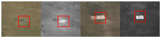
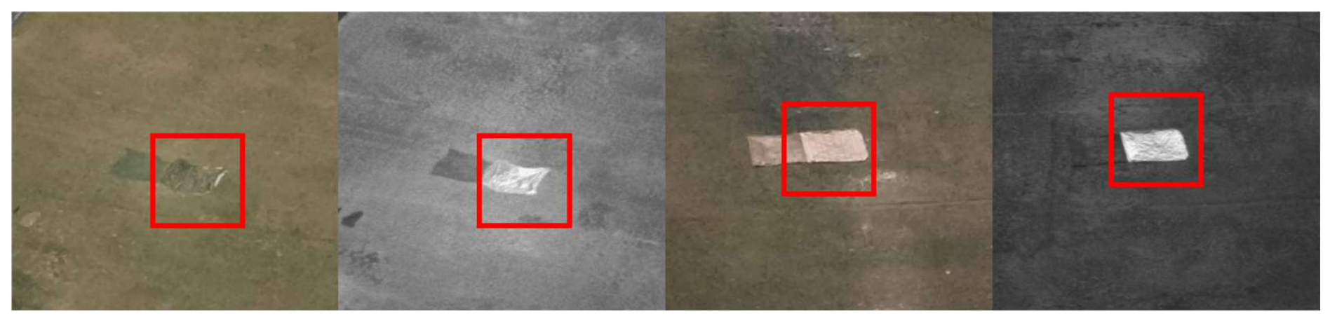
It can be observed that the BRF distributions of these five ground targets are similar in the blue, green, and red bands but show larger differences in the red edge and near-infrared bands [see Figure 10]. In addition, the green camouflage net in Figure 10b exhibits the most similar reflectance pattern to that of natural grassland in Figure 10e. The BRFs based on UAV observation of all five targets vary with view zenith angle and exhibit pronounced hotspot effects. An exception is the yellow camouflage fabric, which shows relatively high BRF at a large view zenith angle, likely due to the material of the fabric and its surface camouflage pattern. Cases where BRF exceeds 1 are also caused by the material properties of the camouflage fabrics. For example, Figure 11 shows bright regions in both the green and yellow camouflage fabrics in the near-infrared band that are visibly noticeable. Although both the camouflage fabrics and nets are made of polyester, differences in manufacturing methods and color patterns result in distinct multispectral characteristics. The surface of the camouflage fabric appears smooth and flat, providing stronger reflectivity. In contrast, the camouflage net has a more complex structure, with a rippled cutting process, inhomogeneous surfaces, and even gaps. Its rough texture produces optical scattering characteristics more similar to the complex three-dimensional structure of grassland.

Figure 11. RGB images and near-infrared band images of the camouflage fabrics. In the left group, the red box highlights the green camouflage fabric. In the right group, the red box highlights the yellow camouflage fabric.

The quantitative analysis was further conducted using the spectral similarity metrics introduced in Section 2.4.2. Taking the multispectral observations of grassland as the background reference, the SAM and RMSESAM values between each type of camouflage fabric/net and the grassland background were calculated for each observation direction using all multiangle observations, and the corresponding mean values are presented in Table 6.

Table 6. Spectral similarity metrics between camouflage fabric/net of different colors and the grassland background. The ground target type corresponding to the bold value is the most similar to grass background.

Ground Target Type	Mean θSAM (°)	Mean RMSESAM
Green Camouflage Fabric	9.645	0.2645
Green Camouflage Net	5.325	0.0440
Yellow Camouflage Fabric	8.271	0.1570
Yellow Camouflage Net	30.129	0.1221

According to the SAM, the spectral-shape similarity with the grass background decreased in the following order: green camouflage net, yellow camouflage fabric, green camouflage fabric, and yellow camouflage net. The green camouflage net exhibited not only the highest similarity in spectral shape to the grassland background but also relatively similar reflectance values. The yellow camouflage fabric showed a certain degree of spectral-shape similarity with the background, although a relatively pronounced difference in reflectance value remained. The green camouflage fabric also exhibited a relatively similar spectral shape to the background, but its reflectance value showed a clear mismatch. Among the four camouflage targets, the yellow camouflage net exhibited the largest spectral difference from the background.

4. Discussion

At present, compared with traditional satellite remote sensing, UAV multiangle observation techniques are being increasingly widely applied. Building on the applicability of BRDF models to high-resolution images, this study investigates the inversion performance of five BRDF models across ten types of ground targets. Overall, the representative results demonstrate that all five BRDF models are capable of representing the optical scattering characteristics of both natural and artificial targets. The influence of the macro-roughness of artificial targets on their BRDF characteristics at extreme VZA should also be considered based on it. Future studies should incorporate high-resolution images and detailed models of the local structural characteristics of artificial targets to perform BRDF inversion. When the CPP + PP dataset is used for inversion, the RMSEs generally fall within acceptable limits. The fitting performance using only the PP dataset is superior to that using only the CPP dataset but slightly inferior to that obtained using the full observation datasets. Owing to differences in model formulation, the inversion performance under different datasets exhibits distinct strengths and limitations across models.

The Walthall model has a relatively simple formulation. Although it accounts for the effect of the azimuth angle, it does not explicitly incorporate the solar zenith angle as a factor influencing bi-directional reflectance. As a result, the model can only describe directional reflectance characteristics under a fixed sun geometry, leading to generally limited capability in reconstructing target BRDF, particularly with deficiencies in hotspot region inversion. The seven-parameter with double-peak model exhibits a distinctive bimodal behavior in the inversion of certain targets, as shown in Figure 6c,d,g. Based on the RMSE and PCC statistics, the RTLSR_C model achieves the best performance when only the CPP dataset is used, despite having the same minimal number of parameters as the Walthall model. Even when faced with the CPP dataset, which contains limited scattering information, the semi-empirical RTLSR_C kernel-driven model maintains high efficiency in utilizing sparse observations. When only the PP dataset is used, the ERPV model performs best, followed by the RTLSR_C model. When only a single-plane dataset is used, the limited number and angular distribution of the observations restrict the HSH model to a second-order representation. The available samples therefore provide insufficient constraints for estimating the HSH coefficients, resulting in an ill-posed inversion and unstable extrapolation over the complete angular domain. In contrast, the combined CPP + PP dataset permits a third-order representation and provides stronger angular constraints; consequently, the HSH model achieves the best performance under the full observation condition, followed by the ERPV model.

Compared with previous studies, this study incorporates a more diverse set of natural and artificial targets, and introduces the camouflage targets as a representative group to investigate multispectral similarity. The dataset we used includes observations in July 2022 at Saihanba, August 2023 in Anyang, and December 2024 in Anyang, with flight altitudes of 200 m, 50 m, and 100 m, respectively. These differences may introduce variations in illumination conditions, vegetation phenology, soil moisture, background composition, and surface structure. Future experiments should use synchronized acquisition campaigns and repeated observations of the same targets under controlled illumination and environmental conditions to provide stronger validation. In addition, the occurrence of BRF greater than 1 for camouflage fabrics should be further investigated in future experiments, as this phenomenon cannot be attributed solely to the intrinsic properties of the materials. Uncertainties associated with the radiometric calibration process may also contribute to BRF values exceeding 1. Future experiments should therefore incorporate more synchronized irradiance measurements and more rigorous radiometric calibration procedures to better quantify and distinguish these potential effects.

The BRDF reconstruction results demonstrate that, even when transitioning from satellite to UAV scale, the five representative BRDF models remain applicable to high spatial resolution images. From the sample-scale variation, it can be observed that the overall trend for the other four models is that RMSE decreases as the sample scale increases, except for the HSH model. At smaller sampling scales, local spatial structures tend to exhibit more complex BRDF characteristics, resulting in relatively higher RMSEs. As the sampling area increases, the spatial heterogeneity associated with local structures is progressively averaged out. And the overall structural characteristics of the targets become smoother. Consequently, the observed BRDF characteristics become more representative of macroscopic reflectance patterns, leading to a decrease in RMSE [19,30]. No clear patterns are observed in reflectance distribution or RMSE across different spectral bands. Analysis of the spectral characteristics of camouflage targets and grassland reveals pronounced differences in reflectance distribution in the non-visible spectral bands. Given the relatively high cost of multispectral observations, the development of low-cost approaches for transforming RGB images into multispectral images holds application potential [34].

5. Conclusions

This study focuses on comparing the inversion capabilities of five representative BRDF models for high-resolution multispectral multiangle images across diverse ground targets. In addition, it extends previous work by incorporating new target types with similar spectral characteristics. The degrees-of-freedom-adjusted RMSE and PCC were used as complementary metrics to evaluate the BRDF reconstruction performance of the five models.

The results indicate that (1) when only the CPP dataset is used, the RTLSR_C model achieves the best inversion performance, whereas the ERPV model performs best when only the PP dataset is used. When the complete CPP + PP dataset is used, the performance of the five models decreases in the following order: HSH, ERPV, RTLSR_C, seven-parameter with double-peak, and Walthall. (2) Although the HSH model performs best when fitted using the complete CPP + PP observations, its performance deteriorates substantially when only single-plane data are available. The limited angular sampling of the CPP-only or PP-only dataset restricts the model to a second-order representation and provides insufficient constraints on the HSH coefficients, resulting in an ill-posed inversion, unstable angular reconstruction, and potentially unrealistic BRF values. (3) The BRDF characteristic of the green camouflage net is most similar to that of grassland. The similarity arises not only from color resemblance, but also from the cutting pattern and loose three-dimensional structure of the net, which produces optical scattering characteristics comparable to those of grassland.

The comparative analysis of model performance provides a basis for selecting appropriate BRDF models in subsequent inversion and fitting research. It offers insights for improving or developing BRDF models tailored to artificial targets with complex three-dimensional structures at a fine scale. Furthermore, incorporating spectral-angle features into camouflage target segmentation models is identified as an important direction for future research.

References

- Strahler, A.H. Vegetation canopy reflectance modeling-recent developments and remote sensing perspectives. Remote Sens. Rev. 1997, 15, 179–194. [Google Scholar] [CrossRef] [Scilit]
- Nicodemus, F.E. Reflectance nomenclature and directional reflectance and emissivity. Appl. Opt. 1970, 9, 1474–1475. [Google Scholar] [CrossRef] [Scilit]
- Qi, J.; Xie, D.; Jiang, J.; Huang, H. 3D radiative transfer modeling of structurally complex forest canopies through a lightweight boundary-based description of leaf clusters. Remote Sens. Environ. 2022, 283, 113301. [Google Scholar] [CrossRef] [Scilit]
- Liu, J.; Fan, W. Review on BRDF model and the inversion strategy. Remote Sens. Technol. Appl. 2008, 23, 104–110. [Google Scholar]
- Minnaert, M.G. The reciprocity principle in lunar photometry. Astrophys. J. 1941, 93, 403–410. [Google Scholar] [CrossRef] [Scilit]
- Hapke, B.W. A theoretical photometric function for the lunar surface. J. Geophys. Res. 1963, 68, 279–280. [Google Scholar] [CrossRef] [Scilit]
- Veverka, J.F.; Wasserman, L.H. Effects of surface roughness on the photometric properties of mars. Icarus 1972, 16, 281–290. [Google Scholar] [CrossRef] [Scilit]
- Pinty, B.; Ramond, D. A simple bidirectional reflectance model for terrestrial surfaces. J. Geophys. Res.-Atmos. 1986, 91, 7803–7808. [Google Scholar] [CrossRef] [Scilit]
- Walthall, C.L.; Norman, J.M.; Welles, J.M.; Campbell, G.; Blad, B.L. Simple equation to approximate the bidirectional reflectance from vegetative canopies and bare soil surfaces. Appl. Opt. 1985, 24, 383–387. [Google Scholar] [CrossRef] [Scilit]
- Bai, L.; Wu, Z.; Zou, X.; Cao, Y. Seven-parameter statistical model for BRDF in the UV band. Opt. Express 2012, 20, 12085. [Google Scholar] [CrossRef] [Scilit]
- Roujean, J.L.; Leroy, M.; Deschanps, P.Y. A bidirectional reflectance model of the Earth’s surface for the correction of remote sensing data. J. Geophys. Res.-Atmos. 1992, 97, 20455–20468. [Google Scholar] [CrossRef] [Scilit]
- Rahman, H.; Pinty, B.; Verstraete, M.M. Coupled surface-atmosphere reflectance (CSAR) model. 2. Semiempirical surface model useable with NOAA advanced very high resolution radiometer data. J. Geophys. Res. 1993, 98, 20791–20801. [Google Scholar] [CrossRef] [Scilit]
- Yang, Y.; Li, W.; Zhang, H. A seven-parameter BRDF model with double-peak characteristic suitable for sandy soil. Math. Probl. Eng. 2018, 2018, 1–8. [Google Scholar] [CrossRef] [Scilit]
- Yang, W.; Qiao, Z.; Li, W.; Ma, X.; Ichii, K. An enhanced RPV model to better capture hotspot signatures in vegetation canopy reflectance observed by the geostationary meteorological satellite Himawari-8. Sci. Remote Sens. 2025, 11, 100222. [Google Scholar] [CrossRef] [Scilit]
- Jiao, Z.; Schaaf, C.B.; Dong, Y.; Román, M.; Hill, M.J.; Chen, J.M.; Wang, Z.; Zhang, H.; Saenz, E.; Poudyal, R. A method for improving hotspot directional signatures in BRDF models used for MODIS. Remote Sens. Environ. 2016, 186, 135–151. [Google Scholar] [CrossRef] [Scilit]
- Dong, Y.; Jiao, Z.; Cui, L.; Zhang, H.; Zhang, X.; Yin, S.; Ding, A.; Chang, Y.; Xie, R.; Guo, J. Assessment of the hotspot effect for the PROSAIL model with POLDER hotspot observations based on the hotspot-enhanced kernel-driven BRDF model. IEEE Trans. Geosci. Remote Sens. 2019, 57, 8048–8064. [Google Scholar] [CrossRef]
- Qin, Z.; Li, X.; Gu, Y. Hemisphere harmonics basis: A universal approach to remote sensing BRDF approximation. IEEE Trans. Geosci. Remote Sens. 2024, 62, 1–12. [Google Scholar] [CrossRef] [Scilit]
- Li, L. Estimation of Vegetation Structural and Optical Variables Using UAV-Based Centimetric Resolution Imagery. Ph.D. Thesis, Beijing Normal University, Beijing, China, 2020. [Google Scholar]
- Zhang, X.; Wang, Y.; Ye, F.; Peng, Z.; Fu, T.; Wang, Z.; Wu, Y.; Wang, Y.; Jiao, Z.; Zhang, H. Accuracy evaluation of fine-scale BRDF archetype inversion considering vegetation structure clustering based on the LESS 3-D simulations at forest scenes. IEEE Trans. Geosci. Remote Sens. 2025, 63, 4415215. [Google Scholar] [CrossRef] [Scilit]
- Kim, M.; Jin, C.; Lee, S.; Kim, K.M.; Lim, J.; Choi, C. Calibration of BRDF based on the field goniometer system using a UAV multispectral camera. Sensors 2022, 22, 7476. [Google Scholar] [CrossRef] [Scilit]
- Cheng, J.; Wen, J.; Xiao, Q.; Hao, D.; Lin, X.; Liu, Q. Exploring the applicability of the semi-empirical BRDF models at different scales using airborne multi-angular observations. IEEE Geosci. Remote Sens. Lett. 2022, 19, 2502905. [Google Scholar] [CrossRef] [Scilit]
- Cao, H.; You, D.; Ji, D.; Gu, X.; Wen, J.; Wu, J.; Li, Y.; Cao, Y.; Cui, T.; Zhang, H. The method of multi-angle remote sensing observation based on unmanned aerial vehicles and the validation of BRDF. Remote Sens. 2023, 15, 5000. [Google Scholar] [CrossRef] [Scilit]
- Xie, J.; Zhang, H.; Pu, J.; Yan, Z.; Cai, Y.; Cui, L.; Cao, H. Multiscale BRDF modeling and scale effect analysis using UAV multiangle remote sensing. IEEE J. Sel. Top. Appl. Earth Obs. Remote Sens. 2025, 18, 23090–23106. [Google Scholar] [CrossRef] [Scilit]
- Yan, Y.; Deng, L.; Liu, X.; Zhu, L. Application of UAV-based multi-angle hyperspectral remote sensing in fine vegetation classification. Remote Sens. 2019, 11, 2753. [Google Scholar] [CrossRef] [Scilit]
- Liu, T.; Abd-Elrahman, A.H. Deep convolutional neural network training enrichment using multi-view object-based analysis of Unmanned Aerial systems imagery for wetlands classification. ISPRS J. Photogramm. Remote Sens. 2018, 139, 154–170. [Google Scholar] [CrossRef] [Scilit]
- Liu, T.; Abd-Elrahman, A.; Dewitt, B.; Smith, S.; Morton, J.; Wilhelm, V.L. Evaluating the potential of multi-view data extraction from small Unmanned Aerial Systems (UASs) for object-based classification for Wetland land covers. GISci. Remote Sens. 2019, 56, 130–159. [Google Scholar] [CrossRef] [Scilit]
- Petracca, I.; Latini, D.; Bonafoni, S.; Frate, F.D.; Giacomo, M.D.; Niro, F. Use of unmanned aerial system for the characterization of the surface reflectance distribution function. In Proceedings of the IEEE International Geoscience and Remote Sensing Symposium (IGARSS), Pasadena, CA, USA, 16–21 July 2023; pp. 4796–4799. [Google Scholar]
- Ye, T.; He, T.; Xu, H.; Ma, Y. Developing an analytical model for neighborhood-scale urban surface bidirectional reflectance incorporating three-dimensional structure. IEEE Trans. Geosci. Remote Sens. 2025, 63, 4505721. [Google Scholar] [CrossRef] [Scilit]
- Ouyang, Y.; Peng, R.; Sha, J.; Zhang, L.; Zhang, K. Hyperspectral camouflage effect evaluation based on spectral indices. J. Appl. Opt. 2023, 44, 523–532. [Google Scholar] [CrossRef] [Scilit]
- Ye, F.; Zhang, X.; Wang, Z.; Wang, Y.; Peng, Z.; Fu, T.; Jiao, Z.; Wu, Y.; Wang, Y.; Dong, Y.; et al. Variation of bi-directional reflectance at multiple spatial resolutions over different land cover types using UAV-based multiangle images. IEEE J. Sel. Top. Appl. Earth Obs. Remote Sens. 2025, 18, 11128–11141. [Google Scholar] [CrossRef] [Scilit]
- Poncet, A.M.; Knappenberger, T.; Brodbeck, C.; Fogle, M.; Shaw, J.N.; Ortiz, B.V. Multispectral UAS data accuracy for different radiometric calibration methods. Remote Sens. 2019, 11, 1917. [Google Scholar] [CrossRef] [Scilit]
- Roman, M.O.; Gatebe, C.K.; Schaaf, C.; Poudyal, R.; Wang, Z.; King, M.D. Variability in surface BRDF at different spatial scales (30 m–500 m) over a mixed agricultural landscape as retrieved from airborne and satellite spectral measurements. Remote Sens. Environ. 2011, 115, 2184–2203. [Google Scholar] [CrossRef] [Scilit]
- Sandmeier, S.R.; Deering, D.W. Structure analysis and classification of boreal forests using airborne hyperspectral BRDF data from ASAS. Remote Sens. Environ. 1999, 69, 281–295. [Google Scholar] [CrossRef] [Scilit]
- Zhang, X.; Peng, Z.; Wang, Y.; Ye, F.; Fu, T.; Zhang, H. A robust multispectral reconstruction network from RGB images trained by diverse satellite data and application in classification and detection tasks. Remote Sens. 2025, 17, 1901. [Google Scholar] [CrossRef] [Scilit]
Disclaimer/Publisher’s Note: The statements, opinions and data contained in all publications are solely those of the individual author(s) and contributor(s) and not of MDPI and/or the editor(s). MDPI and/or the editor(s) disclaim responsibility for any injury to people or property resulting from any ideas, methods, instructions or products referred to in the content. |
© 2026 by the authors. Licensee MDPI, Basel, Switzerland. This article is an open access article distributed under the terms and conditions of the Creative Commons Attribution (CC BY) license.