Sensitivity and Information-Content Assessment of a Candidate Channel Configuration for the Terahertz Ice Cloud Imager Proposed for Next-Generation Fengyun Meteorological Satellites

Highlights

What are the main findings?

• Under both channel-specific and uniform 1 K noise, TICI21 provides more temperature and water-vapor information than ICI11 while retaining comparable frozen-hydrometeor information.
• The small positive ensemble-mean frozen-hydrometeor DFS difference is concentrated mainly in mean-particle-mass states rather than in frozen mass-density states.

What are the implications of the main findings?

• Equal-dimensional 11-observation tests show that the thermodynamic-information gain is not solely attributable to TICI having more observations.
• The six TICI spectral bands provide complementary thermodynamic and frozen-hydrometeor constraints, while forward-model error and footprint co-registration remain to be assessed.

Abstract

Terahertz observations are sensitive to ice-cloud scattering but require thermodynamic context and balanced spectral sampling. This study evaluates a candidate six-band Terahertz Ice Cloud Imager (TICI) configuration for next-generation Fengyun polar-orbiting meteorological satellites. Atmospheric absorption, ice-cloud scattering, and polarization sensitivity below 1 THz are simulated with the Atmospheric Radiative Transfer Simulator. Information content is assessed using 12 Weather Research and Forecasting (WRF)-derived representative composites and 200 individual midlatitude-ocean profiles. The configuration combines water-vapor observations near 183 and 380 GHz, temperature-sensitive observations near the 424 GHz oxygen band, and window observations near 243, 664, and 874 GHz. Compared with the 11-observation Ice Cloud Imager (ICI) reference, the 21-scalar-observation TICI vector provides more temperature and water-vapor degrees of freedom for signal (DFS) under both channel-specific and uniform 1 K noise. Under uniform 1 K noise, the twelve-scene mean frozen-hydrometeor DFS is 4.117 for TICI and 4.034 for ICI; the small increase is concentrated mainly in mean-particle-mass states. Band-removal and equal-dimensional tests show complementary roles for 380, 424, and 874 GHz and indicate that the thermodynamic gain is not solely due to observation count. The conceptual antenna architecture achieves simulated main-beam efficiencies above 95%, while forward-model error, receiver implementation, and footprint co-registration remain to be assessed.

1. Introduction

Clouds can be liquid, ice, or mixed-phase [1]. Ice clouds occur mainly in the upper troposphere and lower stratosphere, typically between 6 and 15 km, and cover 20–50% of the globe [2]. The three-dimensional structure of ice clouds complicates radiative-transfer calculations [3]. Ice-cloud particles are generally nonspherical and span micrometers to millimeters, with their size distributions governed by dynamical and microphysical processes [4]. Because ice clouds affect the Earth’s radiation budget, climate, and severe weather [5], global measurements of their microphysical properties are needed to improve weather and climate models.

Active sensors provide vertically resolved cloud measurements. The 94 GHz CloudSat Cloud Profiling Radar resolves cloud structure at approximately 500 m, while CALIPSO lidar is sensitive to optically thin clouds and cloud tops [6,7]. Their combined observations constrain ice water content and vertical structure, and EarthCARE extends this multisensor approach [8,9]. However, active sensors have limited swath widths and cannot simultaneously provide fine vertical resolution and wide-area imaging.

Passive sensors provide wide-swath coverage. Optical and infrared observations are most sensitive to small particles and optically thin cloud tops, whereas microwave radiometers penetrate deeper into clouds and respond to larger ice particles [5]. Spaceborne microwave imagers and sounders, including GMI, ATMS, and FY-3/MWHS, include channels extending to approximately 183–190 GHz. Polarimetric observations from GMI, MADRAS, and FY-3B/MWHS have shown that scattering by frozen particles and their preferred orientation can produce measurable polarization signatures [10,11,12]. The submillimeter band extends this sensitivity over broader particle-size and altitude ranges. Supplementary Figure S1 illustrates the complementary sensitivity of different spectral regions, and Section 2.2 provides a quantitative comparison under common atmospheric and cloud conditions [13].

Evans et al. [14] proposed spaceborne THz radiometry for ice-cloud sounding, followed by airborne and spaceborne developments from NASA and ESA [15,16,17,18]. IceCube demonstrated observations near 883 GHz, and the Arctic Weather Satellite (AWS) includes channels near 325 GHz [19,20,21]. The nominal AWS 165.5 and 325.15 GHz channels are included in Section 2.2 for a controlled simulation comparison. MetOp-SG(B)/ICI will provide the first operational millimeter/submillimeter radiometer dedicated to ice-cloud observations [22]. Table 1 summarizes the main ICI and IceCube specifications.

Table 1. Main specifications of ICI and IceCube.

Satellite/ Sensor	Central Frequency (GHz)	Polarization	Bandwidth (MHz)	NEDT (K)	Feature
MetOp-SG/ICI	183.31 ± 2.0, 3.4, 7.0	V	1500, 1500, 2000	0.8 K	water vapor lines
	243.2 ± 2.5	H, V	3000	0.7 K	windows
	325.15 ± 1.5, 3.5, 9.5	V	1600, 2400, 3000	1.5, 1.3, 1.2 K	water vapor lines
	448.0 ± 1.4, 3.0, 7.2	V	1200, 2000, 3000	2.0, 1.6, 1.4 K	water vapor lines
	664.0 ± 4.2	H, V	5000	1.6 K	windows
IceCube	883 ± 9	V	6000	0.3 K	windows

Note: For ICI channels specified with ± frequency offsets, the listed bandwidth applies to each of the two symmetric sidebands. The ICI NEDTs are specified at an integration time of 0.6 ms, whereas the IceCube NEDT is specified at an integration time of 1 s. Where multiple bandwidth or NEDT values are given, they correspond to the listed frequency offsets in the same order.

China is conducting feasibility studies for the next-generation Fengyun-5 (FY-5) polar-orbiting satellite series. Its planned morning-orbit mission includes cloud-microphysics observations, providing the mission context for evaluating the Terahertz Ice Cloud Imager (TICI) as a candidate ice-cloud imaging payload [23,24]. For ice-cloud retrieval, the proposed channel configuration combines ice-scattering observations with measurements that constrain the atmospheric temperature and humidity background. The 183 and 380 GHz bands provide humidity sensitivity, while the 424.763 GHz oxygen band provides temperature sensitivity and retains auxiliary ice-cloud sensitivity in its outer wings. The selected bands near 380 and 424.763 GHz also share several frequency offsets with the proposed FY-4 geostationary microwave sounder, which could support future inter-satellite radiance comparisons [25]. This study evaluates a candidate TICI channel configuration through radiative-transfer sensitivity experiments, WRF-based information-content analysis, and conceptual antenna assessment. Section 2, Section 3 and Section 4 present these analyses, and Section 5 summarizes the findings and limitations.

2. Simulating Ice-Cloud Scattering and Atmospheric Gas Absorption in the THz Band

2.1. Model and Data

2.1.1. Atmospheric Radiative Transfer Model

The Atmospheric Radiative Transfer Simulator (ARTS, version 2.6.18) [26] is used to perform radiative transfer simulations of atmospheric ice clouds. Previous studies have evaluated ARTS simulations against airborne observations for cloudy-sky radiative transfer [27] and clear-sky atmospheric absorption [28]. Water vapor, nitrogen, oxygen, and ozone are considered in the gas-absorption calculations. The gaseous absorption by water vapor and oxygen is represented using the ARTS predefined H2O-PWR2022 and O2-PWR2022 models [26,29]. Nitrogen absorption is represented using the N2 self-continuum standard model, and ozone line absorption is calculated using the Perrin spectroscopic line catalog distributed with the ARTS XML data package [30]. The single-scattering properties of ice-cloud particles are obtained from the ARTS single-scattering database [31]. Here, particle habit refers to the particle geometry used to define the single-scattering properties.

For the idealized single-variable sensitivity experiments, a monodisperse size distribution is used to isolate frequency and particle-size effects from variability associated with an assumed particle-size distribution. The scalar ice-cloud experiments in Section 3 and the corresponding supplementary analysis use DISORT [32] with the model-specific IconCloudIce habit (ARTS habit ID 27), represented by oblate-spheroidal particles following the ICON cloud-ice mass–size relationship and assuming totally random orientation [31]. The extended-IWP frequency comparison in Figure 1 uses monodisperse, totally randomly oriented Large Plate Aggregate particles (ARTS habit ID 20). The polarized experiment in Figure 2 uses RT4 with azimuthally random, tilt-resolved single-scattering properties for the same Large Plate Aggregate habit. This habit represents snow in the orientation experiment, whereas cloud ice in the information-content calculations is represented separately using spherical-ice scattering properties. RT4 supplies the vertically and horizontally polarized Planck-equivalent brightness temperatures used to calculate PD in post-processing. Idealized symmetric double-sideband channel responses are used for channels specified by a center frequency and sideband offset; the AWS 165.5 GHz comparison channel is represented by its 2.8 GHz wide single-sideband response.

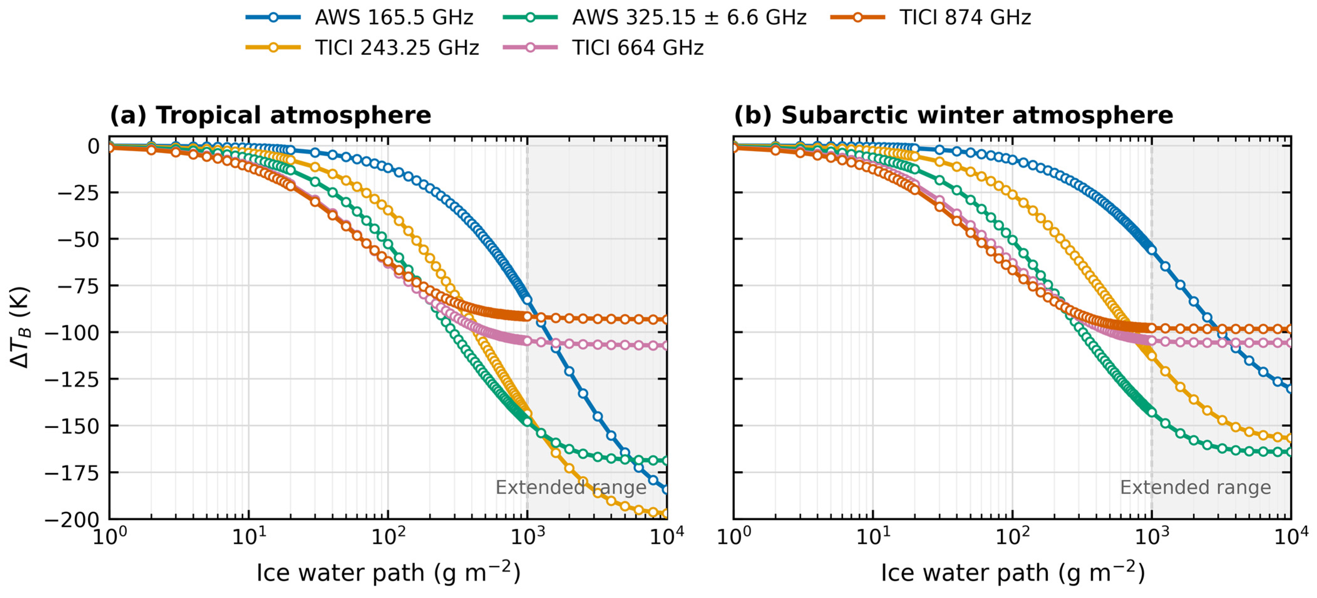
Figure 1. Simulated signed cloud-induced brightness-temperature responses over the extended IWP range for (a) the tropical atmosphere and (b) the subarctic-winter atmosphere. The cloud layer extends from 10 to 11 km and contains monodisperse Large Plate Aggregate particles with $D_{veq}$ = 425.203 μm. The AWS observations are 165.5 GHz and 325.15 ± 6.6 GHz; the TICI observations are 243.25 ± 2.5, 664 ± 4.2, and 874 ± 4.2 GHz. The curves are model-to-model cloudy-sky-minus-clear-sky comparisons, not validation against observations.

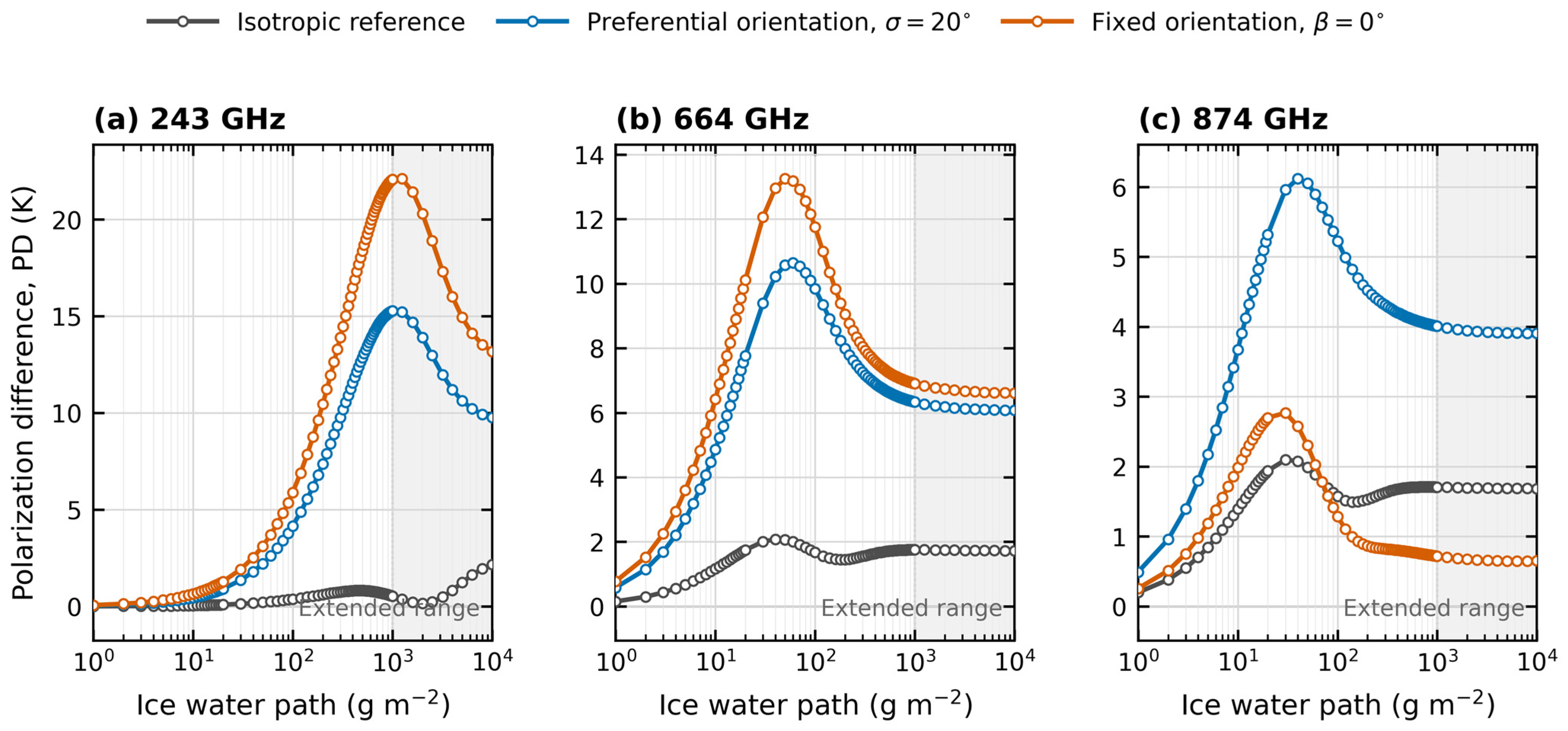
Figure 2. RT4-simulated polarization differences at 243, 664, and 874 GHz for the isotropic reference, the preferential-orientation case ($\sigma ={20}^{\circ }$), and the fixed-orientation case ($\beta =0^{\circ }$) over the extended IWP range. The FASCOD Tropical background and a 10–11 km cloud layer containing monodisperse Large Plate Aggregate particles with $D_{veq}$ = 269.961 μm are used.

For the idealized sensitivity experiments in Section 2 and Section 3, an equal-polarization surface emissivity of 0.6 is adopted as a controlled boundary condition. A fixed surface emissivity of 0.6 has also been adopted in previous millimeter/submillimeter ice-cloud simulations, including the CloudIce study of Buehler et al. [33]. In the WRF-based information-content analysis, a different simplified surface treatment is used, with fixed emissivities of 0.9 over land and 0.6 over ocean, consistent with the ARTS-based millimeter/submillimeter information-content study of Birman et al. [34]. These prescribed values provide consistent boundary conditions for the controlled simulations. More realistic ICI-oriented studies have shown that surface effects and associated emissivity uncertainties can be important for channels with appreciable surface sensitivity [22].

2.1.2. Weather Research and Forecasting (WRF) Model

The WRF model is a mesoscale numerical weather prediction system jointly developed by research centers such as the National Center for Atmospheric Research (NCAR) and the National Centers for Environmental Prediction (NCEP) [35]. In this study, WRF version 4.0 model is used to generate atmospheric profiles for the information-content analysis.

2.1.3. Atmospheric Profile Data

Three atmospheric data sources are used for different purposes in this study. The Fast Atmospheric Signature CODE (FASCOD) provides standardized atmospheric backgrounds for the idealized sensitivity experiments in Section 2 and Section 3; ERA5, the fifth-generation reanalysis produced by the European Centre for Medium-Range Weather Forecasts (ECMWF), provides the initial and boundary conditions for the WRF simulations; and WRF generates physically covarying temperature, humidity, and hydrometeor profiles for the a priori covariance, Jacobian, and information-content calculations.

The idealized simulations use the five standard atmospheres provided by FASCOD [36]: tropical, mid-latitude winter, mid-latitude summer, sub-arctic winter, and sub-arctic summer. Based on these atmospheric backgrounds, prescribed ice-cloud profiles with varying ice water paths (IWP), volume-equivalent particle diameters ($D_{veq}$), and cloud heights are constructed. In Section 2 and Section 3, IWP denotes the prescribed column-integrated ice mass of the idealized single-species cloud layer; it is distinct from the combined WRF frozen-hydrometeor categories used in Section 4. For the standard sensitivity experiments, IWP is sampled at intervals of 1 g m⁻² from 1 to 20 g m⁻², 10 g m⁻² from 30 to 100 g m⁻², and 20 g m⁻² from 120 to 1000 g m⁻², resulting in 73 IWP values. For the extended high-IWP experiment in Section 2.2, this standard grid is supplemented with ten additional values of 1250, 1600, 2000, 2500, 3200, 4000, 5000, 6300, 8000, and 10,000 g m⁻², giving 83 IWP values in total. The $D_{veq}$ values range from 10 to 2929 μm (45 cases), and cloud heights range from 7 to 15 km at 1 km intervals (9 cases). Throughout this sensitivity analysis, cloud height denotes the prescribed cloud-base height of a 1 km thick idealized cloud layer. Thus, the nominal 13 km case extends from 13 to 14 km. Throughout the particle-size sensitivity figures, the axis label “Effective Diameter” refers to the volume-equivalent diameter used in this study.

For the information-content analysis, ERA5 data are used to drive the WRF model. ERA5 provides hourly estimates of atmospheric, oceanic, and land variables at a horizontal resolution of 0.25° × 0.25°, with 37 pressure levels extending to 1 hPa [37]. The resulting WRF simulations provide the atmospheric profiles used to calculate the a priori covariance and Jacobian matrices.

2.2. Ice-Cloud Scattering and Polarization Simulations

Ice-cloud scattering depends on hydrometeor type, particle habit, size, orientation, and wavelength. Preferred orientation of nonspherical particles produces polarization-dependent scattering and can therefore provide information on particle properties [38]. Polarized ice-cloud signals have been observed at microwave frequencies by GMI, MADRAS, and FY-3B/MWHS [10,11,12], and ICI will include dual-polarization observations at 243 and 664 GHz [39].

Radiative-transfer models often assume randomly oriented particles and a macroscopically isotropic ensemble [15,38]. Natural ice particles are commonly nonspherical, however, and sufficiently large particles can develop preferred alignment under gravity, aerodynamic forces, or electrification [38,40,41]. The orientation experiment below therefore compares an isotropic reference with two idealized preferred-orientation cases.

For the RT4 calculations, the particle tilt angle $\beta$ is defined as the angle between the particle symmetry axis and the local vertical. Three orientation states are considered: a randomly oriented isotropic reference, a preferential orientation case with a finite angular spread characterized by $\sigma ={20}^{\circ }$, and an idealized fixed orientation case with $\beta =0^{\circ }$. These orientation states are implemented following the oriented-particle scattering framework described by Brath et al. [38]. Preferred alignment of nonspherical particles modifies the polarization-dependent scattering response, thereby producing differences between the vertically and horizontally polarized brightness temperatures. RT4 provides the vertically and horizontally polarized brightness temperatures, $T_{B,V}$ and $T_{B,H}$, from which the polarization difference (PD) is calculated as

$$PD=T_{B,V}-T_{B,H}.$$

(1)

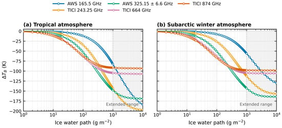
The nonlinear brightness-temperature response at high IWP is examined using the extended 83-point grid defined in Section 2.1.3. Figure 1 uses the FASCOD tropical and sub-arctic winter backgrounds, a monodisperse Large Plate Aggregate particle with $D_{veq}$ = 425.203 μm, a cloud layer extending from 10 to 11 km, a surface emissivity of 0.6, an 820 km sensor altitude, and a 53° incidence angle. The simulated channels are AWS 165.5 GHz and 325.15 ± 6.6 GHz; the TICI window channels are 243.25 ± 2.5, 664 ± 4.2, and 874 ± 4.2 GHz; the bandwidths of the three TICI window observations are 3, 4, and 4 GHz, respectively. Within each atmospheric background, the cloudy and clear calculations otherwise use identical settings. The signed cloud-induced response is defined as

$$\Delta T_B=T_{B,cloud}-T_{B,clear}.$$

(2)

Figure 1 shows the signed $\Delta T_B$ as a function of IWP for the tropical and subarctic-winter atmospheric backgrounds; negative values denote cloud-induced cooling. The curves compare cloudy-sky and clear-sky simulations under otherwise identical model settings. Their magnitude and ordering vary with IWP, frequency, and atmospheric background, so no single saturation threshold or fixed frequency ranking applies across all tested conditions.

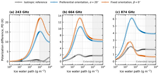
Particle-orientation effects are examined with RT4 at 243, 664, and 874 GHz using the FASCOD tropical background, the extended 83-point IWP grid, a 10–11 km cloud layer, a monodisperse Large Plate Aggregate particle with $D_{veq}$ = 269.961 μm, a surface emissivity of 0.6, an 820 km sensor altitude, and a 53° incidence angle (Figure 2). At 243 GHz, PD reaches 15.3 K for the preferential-orientation case and 22.1 K for the fixed-orientation case, with maximum increments of 14.9 and 21.7 K relative to the isotropic reference. At 664 GHz, both oriented cases produce larger PD than the isotropic reference, with maximum increments of 8.6 and 11.2 K, respectively. At 874 GHz, the preferential-orientation case has a maximum increment of 4.1 K, whereas the difference between the fixed-orientation case and the isotropic reference changes from positive at lower IWP to negative at higher IWP. Particle orientation therefore changes both the magnitude and IWP dependence of the polarization response across frequencies.

2.3. Water Vapor Absorption Bands

Supplementary Figure S2 shows the simulated clear-sky brightness temperatures for four water vapor channels under different atmospheric profiles and frequency offsets. It can be seen that the TB spectra at 183 GHz and 325 GHz exhibit similar shapes, while those at 380 GHz and 448 GHz also show similar spectral characteristics. Previous studies have demonstrated the capability of the 183 GHz channel for ice cloud measurements [42,43,44]. In this paper, we adopt the same five 183 GHz frequency offsets as those used by MWHS-II. Four of the six 380.1974 GHz offsets coincide with the candidate FY-4M geostationary microwave channel set [25], while the full TICI set extends from the line core to the wings to sample humidity-background and ice-cloud responses.

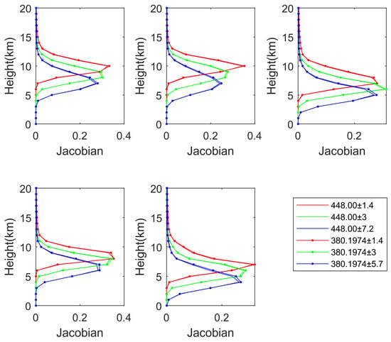
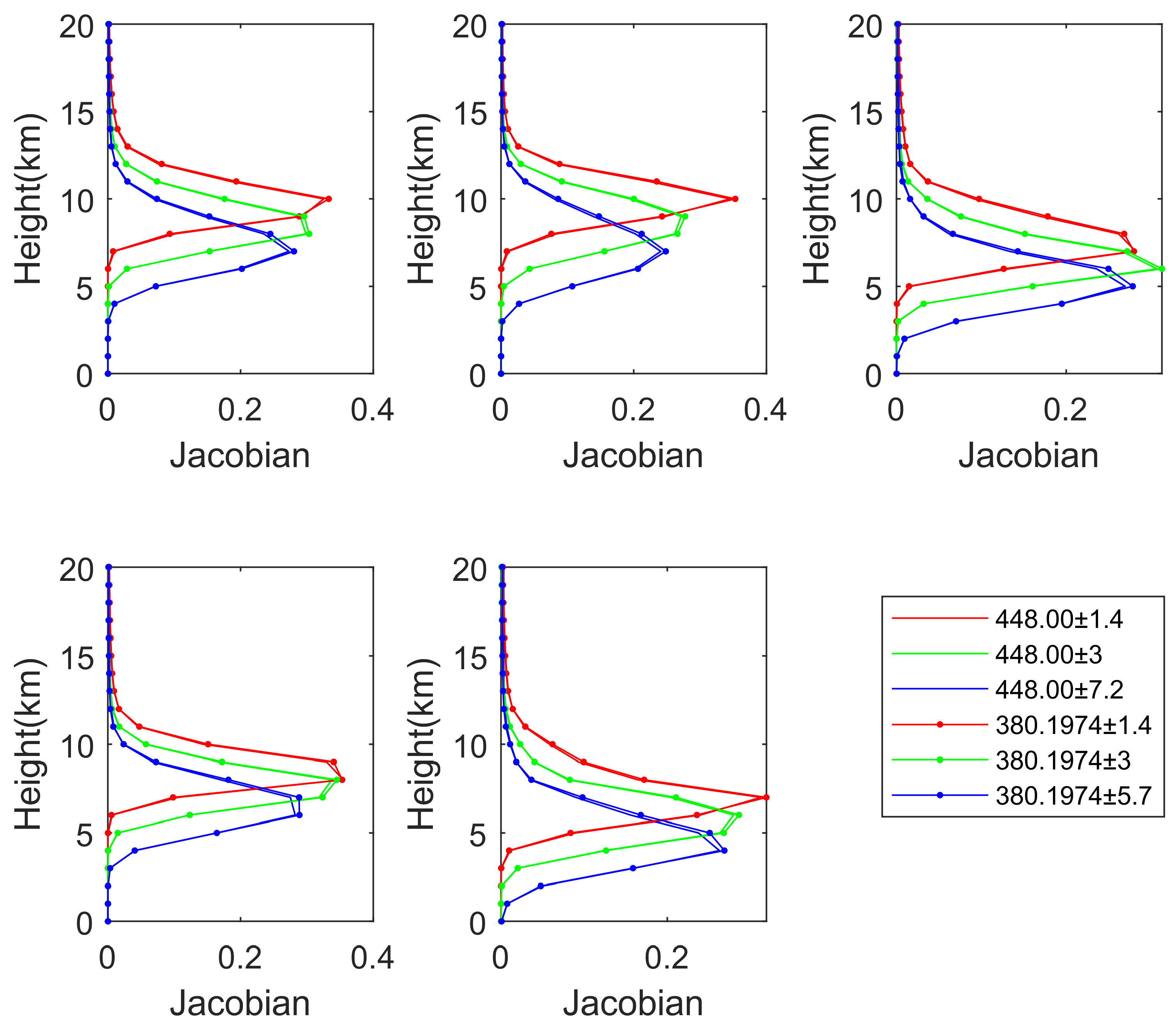
Table 2 compares matched 380 and 448 GHz observations, with the 380 GHz offsets selected to minimize the absolute difference between their mean clear-sky TBs across the five FASCOD standard atmospheres. These matched offsets are used only for the spectral comparison. The signed paired difference is defined as TB380 GHz−TB448 GHz. The differences are small near the line center and increase toward the wings, while the corresponding temperature Jacobians in Figure 3 show broadly similar vertical sensitivity. These results support 380 GHz as a candidate TICI band. Mean and STD denote the mean and standard deviation of the signed differences across the five profiles.

Table 2. Matching results for the 380 GHz channel and the 448 GHz channel.

Channel (GHz)	Bandwidth (MHz)	Channel (GHz)	Bandwidth (MHz)	Mean (K)	STD (K)
448.00 ± 1.4	1200	380.1974 ± 1.4	600	0.20	0.04
448.00 ± 3	2000	380.1974 ± 3	800	0.19	0.09
448.00 ± 7.2	3000	380.1974 ± 5.7	4000	0.429	0.12

Figure 3. Temperature Jacobians (∂TB/∂T, K K⁻¹) for each matched channel at 380 GHz and 448 GHz. Red, green, and blue denote the three matched channel pairs listed in Table 2. Curves with and without circular markers represent the 380.1974 and 448 GHz observations, respectively.

2.4. Oxygen Absorption Bands

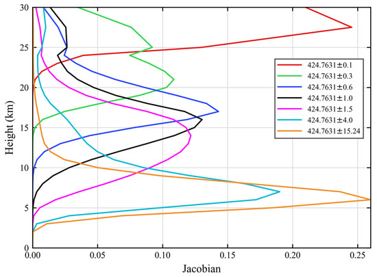
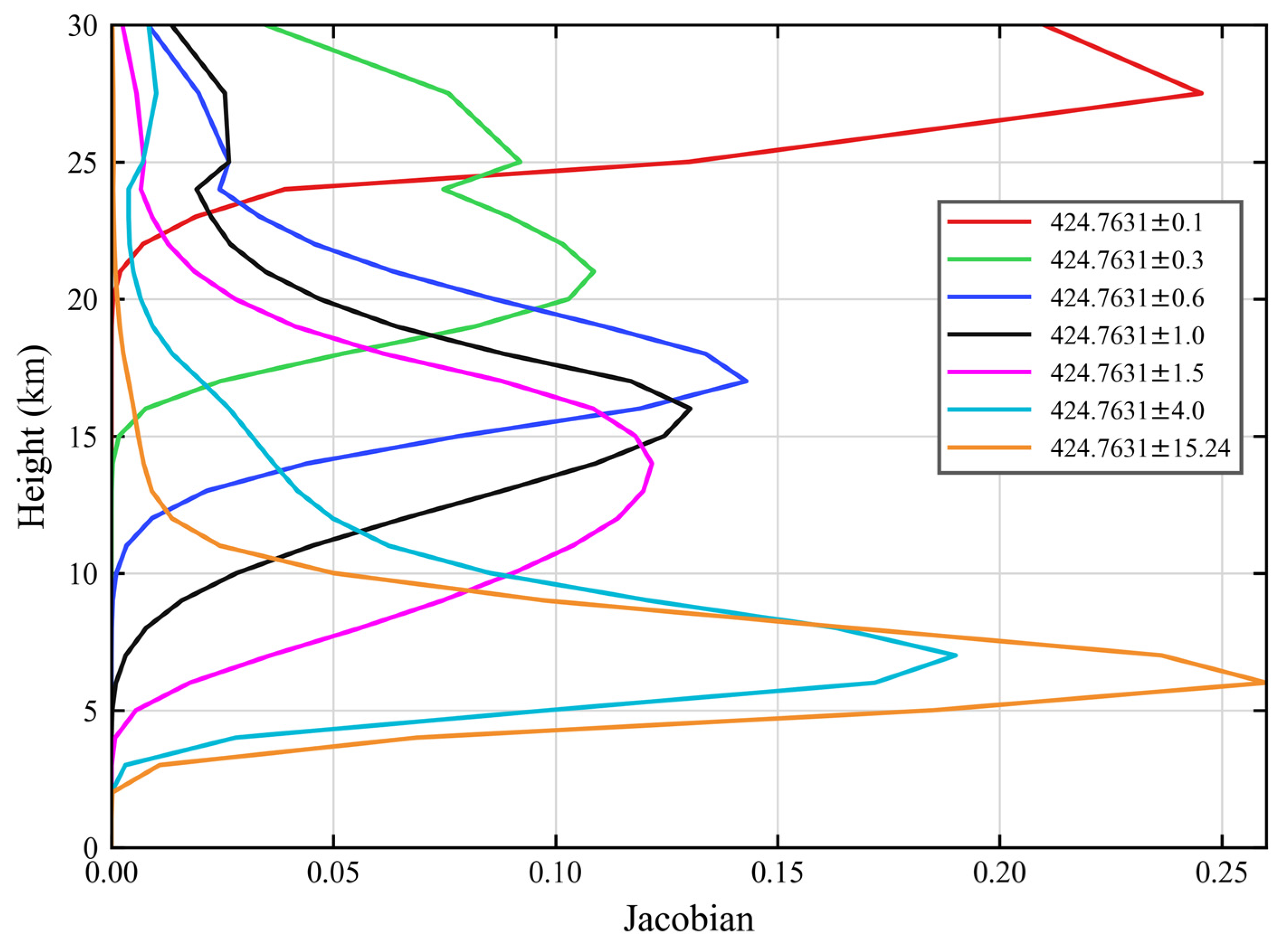
Supplementary Figure S3 compares clear-sky TBs near the 118.75 and 424.7631 GHz oxygen bands across atmospheric profiles and frequency offsets. At 424.7631 GHz, the ±0.3, ±0.6, ±1.0, ±1.5, and ±4.0 GHz offsets coincide with the candidate FY-4M channel set [25], while TICI additionally includes observations at ±0.1 and ±15.24 GHz. The inner offsets provide sensitivity to the temperature background, whereas the outer offsets retain sensitivity to ice-cloud scattering. Figure 4 shows the corresponding temperature Jacobians. Accordingly, Section 4 includes temperature in the atmospheric-background state used for the information-content analysis.

Figure 4. Temperature Jacobian (∂TB/∂T, K K⁻¹) for different channels at 424 GHz in the tropical atmosphere.

3. TICI Channels and Sensitivity Analysis

3.1. TICI Channels

The candidate TICI configuration follows three principles [5,45]: absorption channels should limit surface influence and avoid strong interfering lines; widely separated frequencies should sample different ice-particle sizes; and offsets within absorption bands should provide complementary vertical and thermodynamic sensitivity. Clear- and cloudy-sky TBs, atmospheric transmittance, and weighting functions are used to select the center frequencies, offsets, and bandwidths.

Based on the simulation analyses presented, the 243, 664, and 874 GHz window bands provide complementary ice-cloud sensitivity under different IWP conditions, together with polarization sensitivity to particle orientation. The 183 and 380 GHz water-vapor bands provide humidity-background sensitivity, whereas the 424 GHz oxygen band provides temperature-background sensitivity. In the candidate configuration, channels at different frequency offsets within the absorption bands are retained to examine ice-cloud sensitivity from near-line to quasi-window conditions. The resulting candidate channel configuration is summarized in Table 3.

Table 3. Candidate TICI channel configuration. H and V denote horizontal and vertical polarization, respectively.

Channel	Frequency (GHz)	Bandwidth (MHz)	NEDT (K)	Polarization
1	183.31 ± 1	500	0.9	H
2	183.31 ± 1.8	1000	0.7	H
3	183.31 ± 3	1000	0.7	H
4	183.31 ± 4.5	1500	0.6	H
5	183.31 ± 7	2000	0.6	H
6	243.25 ± 2.5	3000	0.8	V
7	243.25 ± 2.5	3000	0.8	H
8	380.1974 ± 0.045	30	6.1	H
9	380.1974 ± 0.4	200	2.5	H
10	380.1974 ± 1.5	500	1.6	H
11	380.1974 ± 4.0	900	1.4	H
12	380.1974 ± 9.0	2000	1.2	H
13	380.1974 ± 18.0	2000	1.2	H
14	424.7631 ± 0.1	100	5.3	H
15	424.7631 ± 0.3	100	5.3	H
16	424.7631 ± 0.6	200	3.7	H
17	424.7631 ± 1.0	400	2.6	H
18	424.7631 ± 1.5	600	2.1	H
19	424.7631 ± 4.0	2000	1.6	H
20	424.7631 ± 15.24	3000	1.3	H
21	664.0 ± 4.2	4000	1.5	V
22	664.0 ± 4.2	4000	1.5	H
23	874.0 ± 4.2	4000	1.9	V
24	874.0 ± 4.2	4000	1.9	H

Table 3 lists 24 channel-polarization entries representing 21 distinct spectral settings because the 243, 664, and 874 GHz settings each include a co-frequency V/H pair. For the scalar information-content analysis, each V/H pair is represented by one Planck-equivalent Stokes-I observation, yielding the TICI21 observation vector. Polarization differences are evaluated separately and are not included in the present DFS calculation. Applying the same representation to the 243 and 664 GHz pairs reduces the 13-entry ICI reference to ICI11. The tabulated NEDT is assigned directly to each scalar observation without a square-root-of-two reduction.

3.2. Sensitivity Analysis of TB to Ice Cloud Parameters

3.2.1. Sensitivity of TB to Cloud Height

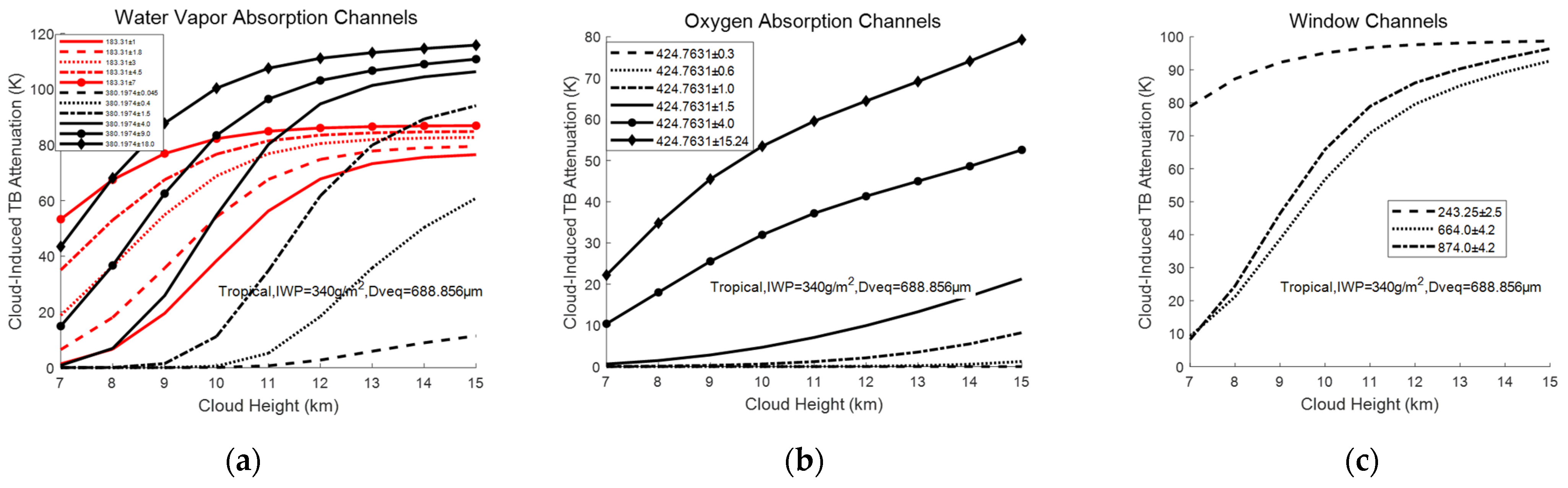
Figure 5, Figure 6 and Figure 7 and Supplementary Figures S4–S6 use positive cloud-induced TB attenuation, defined as the clear-sky minus cloudy-sky TB and therefore opposite in sign to Equation (2). In Figure 5a, attenuation increases toward the outer water-vapor-band offsets for the prescribed tropical cloud, and the 380 GHz observations retain height sensitivity after the 183 GHz responses begin to flatten. The 380.1974 ± 18 GHz observation has the strongest height response within these bands.

Figure 5. Positive cloud-induced brightness-temperature attenuation as a function of prescribed cloud-base height for (a) water-vapor absorption channels, (b) oxygen-absorption channels, and (c) window channels. Attenuation is defined as the clear-sky minus cloudy-sky brightness temperature and is opposite in sign to the signed response in Equation (2).

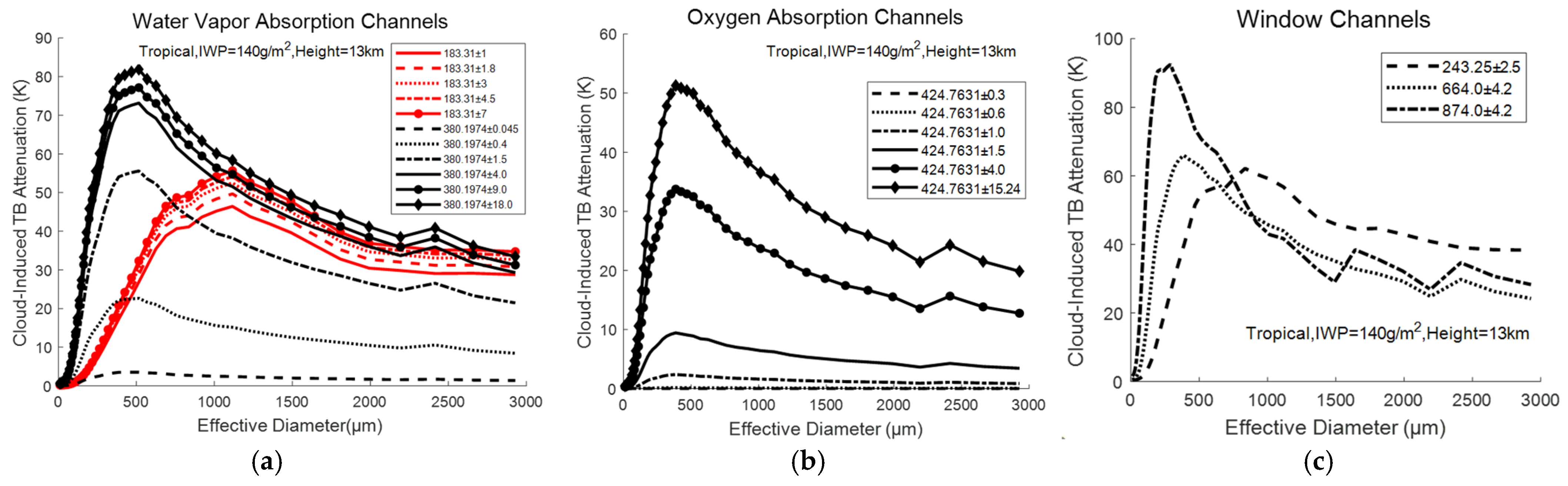
Figure 6. Positive cloud-induced brightness-temperature attenuation as a function of volume-equivalent particle diameter for (a) water-vapor absorption channels, (b) oxygen-absorption channels, and (c) window channels.

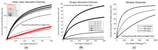
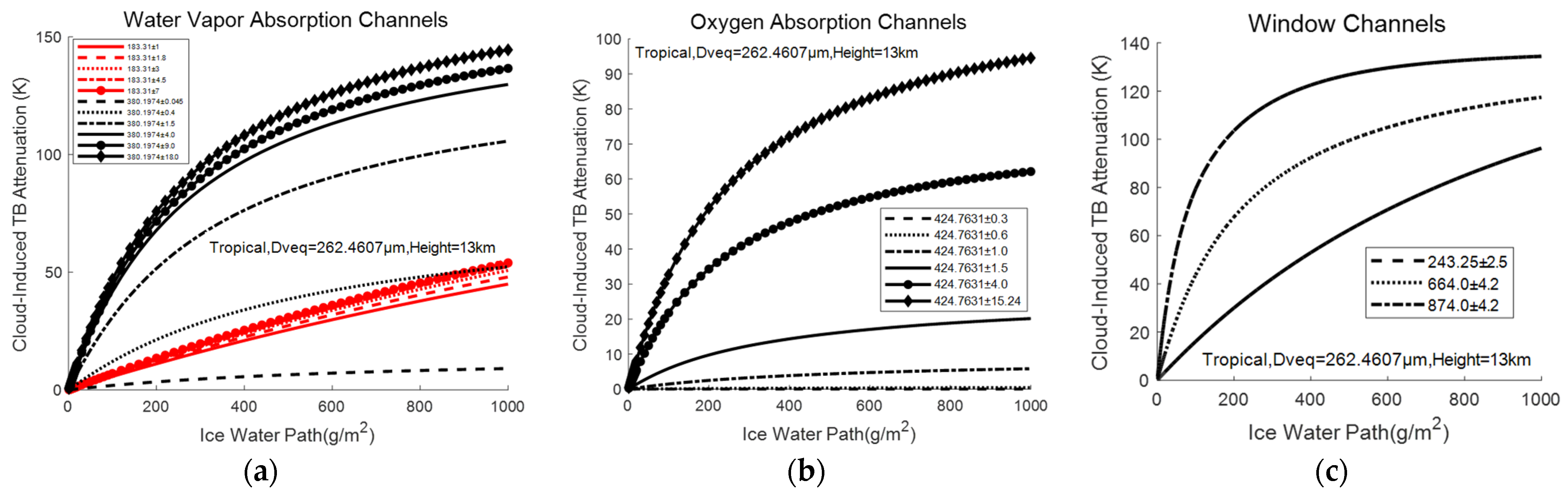
Figure 7. Positive cloud-induced brightness-temperature attenuation as a function of IWP for a fixed tropical cloud case with a cloud-base height of 13 km and a volume-equivalent particle diameter of 262.4607 μm: (a) water-vapor absorption channels, (b) oxygen-absorption channels, and (c) window channels.

For the 424 GHz band, attenuation also increases toward the outer offsets (Figure 5b). The ±15.24 GHz observation has a pronounced height response, whereas the inner observations remain dominated by temperature sensitivity. For the window observations (Figure 5c), the 243 GHz response changes little above about 10 km, while the 664 and 874 GHz responses continue to vary. The outer 380 and 424 GHz observations also retain strong height sensitivity, demonstrating complementary responses across the candidate bands.

Overall, the relative channel responses vary across the prescribed 7–15 km range, so the multi-band configuration provides complementary rather than uniformly ordered sensitivity to cloud height. The cloud-height experiments are limited to 7–15 km and therefore characterize tropospheric and upper-tropospheric ice clouds; higher-altitude polar stratospheric clouds are outside the range considered here.

3.2.2. Sensitivity of TB to Volume-Equivalent Particle Diameter

Figure 6 compares positive cloud-induced brightness-temperature attenuation as a function of volume-equivalent particle diameter under a tropical atmosphere, with IWP fixed at 140 g m⁻² and the cloud-base height fixed at 13 km. For the absorption bands, attenuation generally increases toward the outer frequency offsets. As frequency increases, the response peaks generally shift toward smaller $D_{veq}$. Beyond the peak, attenuation usually decreases with increasing particle size, although appreciable responses can persist at larger diameters and the post-peak behavior remains channel-dependent. The peak locations and subsequent changes are specific to the prescribed atmospheric and cloud conditions and are not interpreted as threshold-defined sensitivity limits.

3.2.3. Sensitivity of TB to IWP

Figure 7 shows positive attenuation as a function of IWP for a fixed tropical cloud with a 13 km cloud base and $D_{veq}$ = 262.4607 μm. The three panels group the water-vapor, oxygen, and window observations. Attenuation generally increases with IWP, but the response is nonlinear and channel-dependent.

Supplementary Figures S4–S6 show the joint dependence on IWP and $D_{veq}$ at a 13 km cloud base. Sensitivity increases toward the outer offsets of the 380 GHz band. At 424 GHz, the ±4 and ±15.24 GHz observations retain ice-scattering sensitivity, whereas the inner observations remain dominated by the temperature background. The cloud-height, particle-size, and IWP experiments were repeated with the FASCOD subarctic-winter atmosphere using the same cloud and radiative-transfer settings; the results are provided in Supplementary Figures S7–S9. The tropical and supplementary subarctic-winter results show that atmospheric background changes both response magnitude and channel ordering; Figure 5, Figure 6 and Figure 7 and Supplementary Figures S4–S6 therefore describe the prescribed tropical atmosphere rather than globally invariant ranges.

4. Information Content Analysis of TICI

4.1. Calculation Method

Information content measures the reduction in state uncertainty provided by an observation vector. This study uses degrees of freedom for signal (DFS), rather than entropy reduction, to quantify the information supplied by TICI [46].

Assuming the state vector contains n atmospheric state parameters, the total DFS is defined as the expected normalized reduction from the a priori state to the posterior state:

$$DFS=E\left[{\left({\mathit{x}}_p-{\mathit{x}}_a\right)}^T{\mathit{S}}_a^{-1}\left({\mathit{x}}_p-{\mathit{x}}_a\right)\right]=trace\left(\mathit{I}-{\mathit{S}}_p{\mathit{S}}_a^{-1}\right),$$

(3)

where ${\mathit{x}}_a$ and ${\mathit{x}}_p$ denote the a priori and posterior state estimates, respectively; $\mathit{I}$ denotes the identity matrix, ${\mathit{S}}_a$ represents the a priori error covariance matrix, and ${\mathit{S}}_p$ is the posterior error covariance matrix. According to optimal estimation theory, the posterior error covariance matrix is given by

$${\mathit{S}}_p={\left({\mathit{S}}_a^{-1}+{\mathit{J}}^T{\mathit{S}}_{\epsilon }^{-1}\mathit{J}\right)}^{-1},$$

(4)

where ${\mathit{S}}_{\epsilon }$ represents the adopted observation-error covariance matrix. $\mathit{J}$ denotes the Jacobian matrix, reflecting the sensitivity of channels to retrieval parameters. The averaging-kernel matrix is defined as $\mathit{A}=\mathit{I}-{\mathit{S}}_p{\mathit{S}}_a^{-1}$. For a specified group of state variables, its DFS is obtained by summing the corresponding diagonal elements of the averaging-kernel matrix.

DFS depends on the a priori covariance ${\mathit{S}}_a$, the observation-error covariance ${\mathit{S}}_{\epsilon }$, and the Jacobian $\mathit{J}$. Here, ${\mathit{S}}_a$ is estimated from ERA5-driven WRF profiles, $\mathit{J}$ is calculated with ARTS, and ${\mathit{S}}_{\epsilon }$ is specified from the adopted channel-noise assumptions.

4.2. Information Content Analysis Setup

4.2.1. Simulation Construction

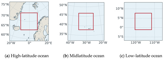
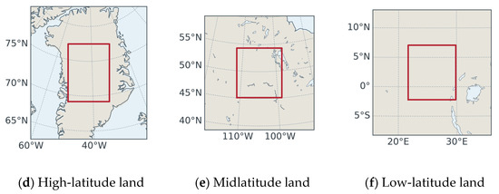
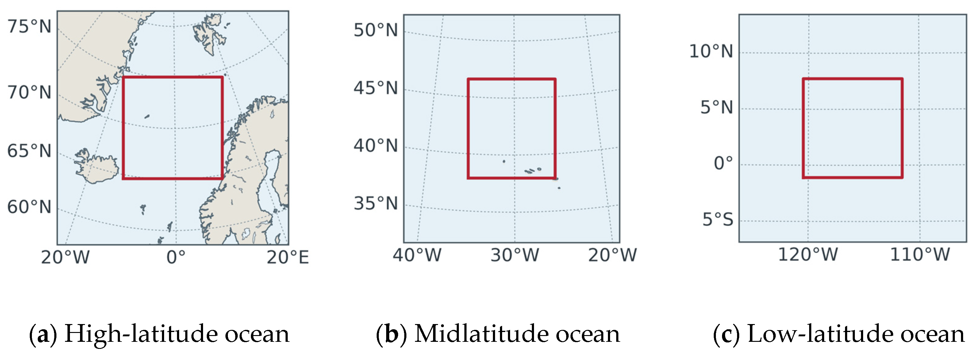
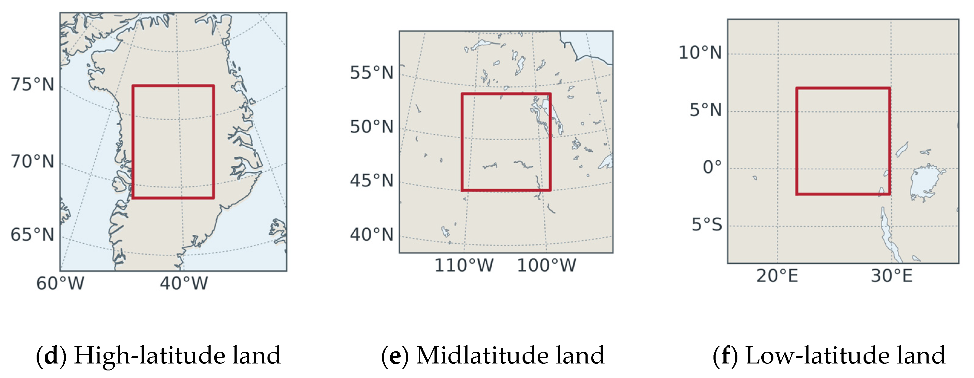
ERA5-driven WRF simulations for January and July 2014 are sampled over high-, mid-, and low-latitude ocean and land regions, defining 12 atmospheric scene classes. Table 4 lists the domain centers and grid dimensions, and Figure 8 shows their locations. WRF uses 10 km horizontal resolution, 29 vertical levels, a 50 hPa model top, and a 60 s time step; the profiles are mapped to a 55-level computational grid for radiative-transfer and information-content calculations. RRTMG radiation [47], the YSU boundary-layer scheme [48], Milbrandt two-moment microphysics [49,50], and Kain–Fritsch convection [51] are used. WRF supplies mass and number mixing ratios for cloud liquid water, rain, cloud ice, snow, graupel, and hail.

Table 4. The study regions.

Surface Type	Latitude	No.	Region Center (Latitude, Longitude; °)	Grids
Ocean	High	1	[70.269, −0.64]	109 × 112
	Mid	2	[42.538, −30.326]	86 × 98
	Low	3	[3.342, −116.006]	100 × 100
Land	High	4	[73.557, −41.792]	67 × 93
	Mid	5	[50.004, −104.896]	94 × 103
	Low	6	[2.453, 25.757]	92 × 105

Figure 8. Geographical locations of the six WRF study regions. Panels (a–f) correspond to regions 1–6 listed in Table 4, respectively. Red outlines indicate the WRF domains; beige and blue denote land and water, respectively.

For each hydrometeor species, mean particle mass is the ratio of WRF mass to number mixing ratio where mass exceeds 10⁻¹⁶ kg kg⁻¹ and number is positive. Profiles with inconsistent mass and number mixing ratios are excluded. Numerical floors of 10⁻¹² kg m⁻³ and 10⁻¹⁸ kg are applied to hydrometeor mass density and mean particle mass, respectively, before the ${\mathrm{l}\mathrm{o}\mathrm{g}}_{10}$ transformation.

One WRF-statistical representative composite was constructed for each of the 12 scene classes. Two additional 100-profile ensembles from the January and July midlatitude-ocean scenes were selected deterministically to evaluate profile-level variability and seasonal consistency, as described in Section 4.2.5. Each representative composite uses profiles with total frozen-hydrometeor path ≥0.1 kg m⁻² after removal of the upper 0.5% tail. Temperature and water vapor are taken from a multivariate WRF medoid. The median frozen path is partitioned by mean species mass fraction, while cloud-liquid-water and rain paths use occurrence-conditioned 75^th percentiles from the broader population with frozen path ≥0.01 kg m⁻². Hydrometeor vertical structures are robust averages of path-normalized profiles, and mean-particle-mass profiles are density-weighted geometric means within the scattering-property support ranges.

4.2.2. A Priori Error Covariance Matrix

The a priori error covariance matrix ${\mathit{S}}_a$ contains the variances and cross-covariances of the state variables. For $n$ state variables $x_1$,$x_2$,…,$x_n$, it is expressed as

$${\mathit{S}}_a=\left[\begin{array}{ccc}cov\left(x_1,x_1\right)& cov\left(x_1,x_2\right)& \begin{array}{cc}\dots & cov\left(x_1,x_n\right)\end{array}\\ cov\left(x_2,x_1\right)& cov\left(x_2,x_2\right)& \begin{array}{cc}\dots & cov\left(x_2,x_n\right)\end{array}\\ \begin{array}{c}\dots \\ cov\left(x_n,x_1\right)\end{array}& \begin{array}{c}\dots \\ cov\left(x_n,x_2\right)\end{array}& \begin{array}{c}\begin{array}{cc}\dots & \dots \end{array}\\ \begin{array}{cc}\dots & cov\left(x_n,x_n\right)\end{array}\end{array}\end{array}\right],$$

(5)

For a dataset containing $m$ samples, the unregularized sample covariance is defined as

$$cov\left(x_i,x_j\right)={\displaystyle \frac{1}{m-1}}{\displaystyle {\sum }_{k=1}^m}\left(x_i^k-\overline{x_i}\right)\left(x_j^k-\overline{x_j}\right),$$

(6)

where $\overline{x_i}$ and $\overline{x_j}$ are the sample means of $x_i$ and $x_j$, respectively. Retaining interlevel and intervariable correlations is important because neglecting them may alter the estimated posterior uncertainty and DFS [52,53].

The state vector contains 14 variable blocks on the 55-level grid, giving 770 elements: temperature, water vapor, six hydrometeor mass densities, and six corresponding mean particle masses. Temperature is represented in linear space; all other variables are represented in log10 space. A separate ${\mathit{S}}_a$ is estimated for each scene class from WRF profiles with total frozen-hydrometeor path ≥0.01 kg m⁻². The high-dimensional sample covariance is regularized using Oracle Approximating Shrinkage [54], and Sa and J use the same state-variable and vertical-level ordering.

The corresponding correlation matrix is defined as

$$C\left(i,j\right)={\displaystyle \frac{{\mathit{S}}_a\left(i,j\right)}{\sqrt{{\mathit{S}}_a\left(i,i\right){\mathit{S}}_a\left(j,j\right)}}}.$$

(7)

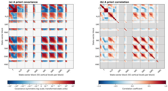
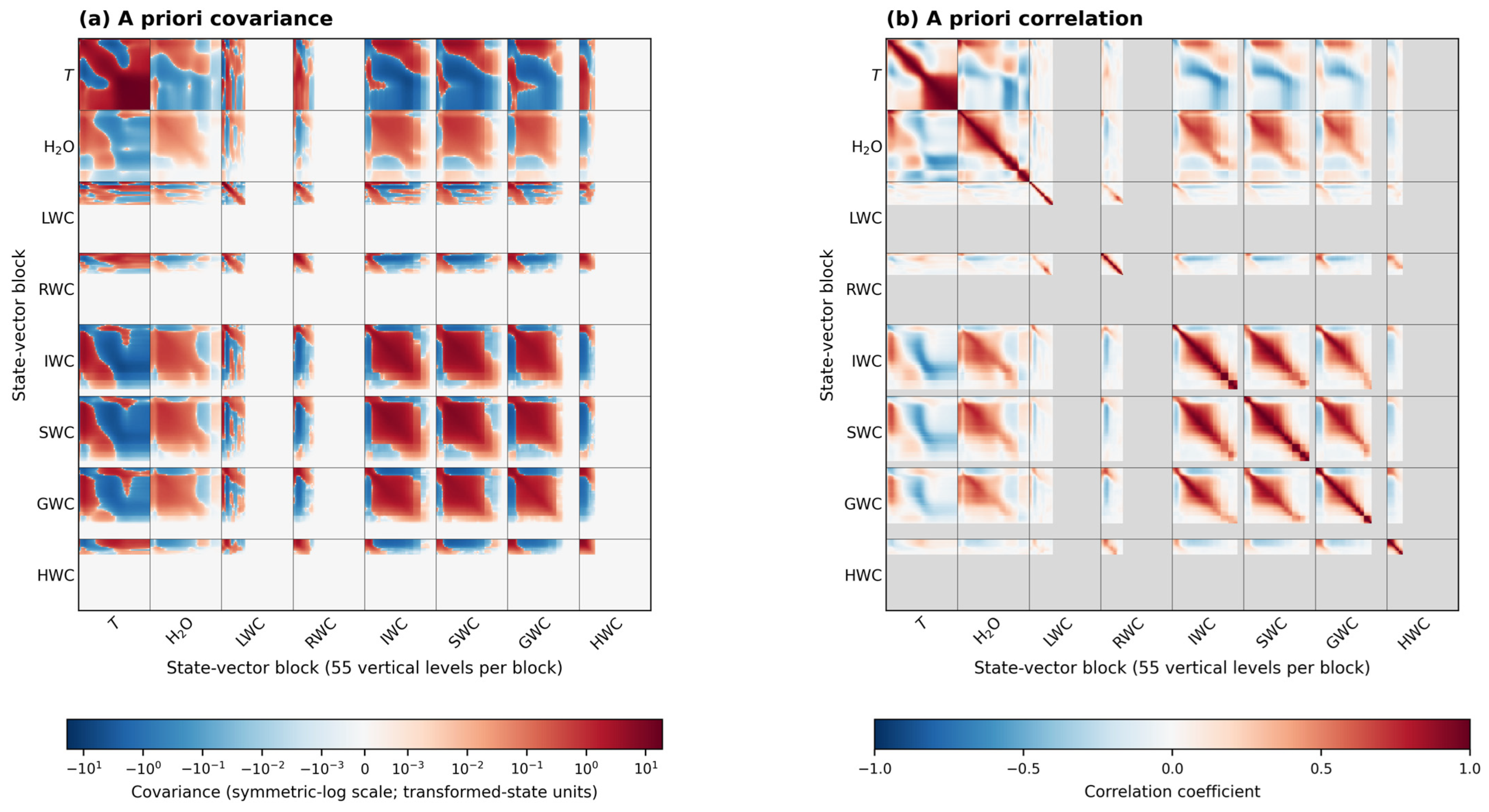
Figure 9 shows the January high-latitude-ocean covariance and correlation structures. Temperature, water vapor, and frozen hydrometeors exhibit vertical and cross-variable correlations, while sparse liquid-water, rain, and hail regions reflect limited occurrence. Mean-particle-mass blocks are omitted from the figure but retained in the 770-element calculation. These covariances represent the January and July 2014 WRF populations rather than climatology; finite samples, limited temporal coverage, and WRF dependence may affect absolute DFS.

Figure 9. A priori (a) covariance and (b) correlation matrices for the January high-latitude-ocean scene. The six mean-particle-mass blocks are omitted from the visualization for clarity but remain included in the complete state vector and DFS calculations.

4.2.3. Observation-Error Covariance Matrix

The observation-error covariance matrix ${\mathit{S}}_{\epsilon }$ can represent both instrumental noise and forward-model error. In this study, it includes only channel noise represented by the noise-equivalent delta temperature (NEDT). Forward-model uncertainties associated with gas absorption, surface emissivity, particle scattering properties, particle-size distributions, and cloud structure are not explicitly included. In particular, uncertainty associated with the prescribed surface-emissivity assumptions described in Section 2.1.1 is not represented in ${\mathit{S}}_{\epsilon }$.

Channel-noise errors are assumed to be independent among scalar observations. Accordingly, ${\mathit{S}}_{\epsilon }$ is represented as a diagonal matrix:

$${\mathit{S}}_{\epsilon ,ij}=\left\{\begin{array}{cc}{\sigma }_i^2,& i=j,\\ 0,& i\ne j,\end{array}\right.$$

(8)

where ${\sigma }_i$ is the NEDT of scalar observation $i$. The diagonal elements of ${\mathit{S}}_{\epsilon }$ are therefore noise variances expressed in K². The nominal radiometric sensitivity is given by

$$NEDT={\displaystyle \frac{T_{sys}}{\sqrt{B\tau }}},$$

(9)

where $T_{\mathrm{s}\mathrm{y}\mathrm{s}}$ is the system noise temperature, $B$ is the observation bandwidth, and $\tau$ is the integration time. The nominal channel-specific NEDTs adopted as design assumptions for the complete-configuration analysis are listed in Table 1 and Table 3; they are not presented as measured receiver performance.

Complete TICI21 and ICI11 are compared using their respective channel-specific NEDTs: the ICI11 values are taken from Table 1 and the TICI21 values from Table 3. They are also compared under uniform independent 1 K noise, which equalizes per-observation noise but not vector dimension. Band-removal, channel-removal, and equal-dimensional replacement experiments use uniform 1 K noise.

4.2.4. Jacobian Matrix $\mathit{J}$

The Jacobian matrix $\mathit{J}=\partial \mathit{y}/\partial \mathit{x}$ describes the local sensitivity of the scalar brightness-temperature observation vector $\mathit{y}$ to the atmospheric state vector $\mathit{x}$. The Jacobians were evaluated at the twelve representative composites and at each individual profile used in the two profile-level ensembles.

The calculations assume an 820 km orbit, a 53° incidence angle, and the channel specifications in Table 3. Scalar information-content simulations use ARTS 2.6.18 with DISORT and randomly oriented particles. Liquid water and rain are spherical; cloud ice uses spherical-ice properties; snow uses the Large Plate Aggregate habit; and graupel and hail use the ICON graupel and ICON hail scattering datasets, respectively. Hydrometeor mass density and mean particle mass determine the modified-gamma-distribution normalization and scale, with fixed shape parameters $\mu$ and $\gamma$ from Table 5 [55]. TICI and ICI use identical profiles, surfaces, hydrometeor states, absorption models, and radiative-transfer settings.

Table 5. Parameters for the size distribution function.

Hydrometeor	$\mathit{\mu }$	$\mathit{\gamma }$
cloud liquid water	1	1
rain	0	1/3
cloud ice	0	1/3
snow	0	1/2
graupel	1	1/3
hail	1	1/3

The Jacobian matrix is evaluated using one-sided finite differences by perturbing one state element while holding all other elements fixed. For observation $m$ and state element $x_j$,

$$J_{m,j}\approx {\displaystyle \frac{F_m\mathrm{ }\left(\mathit{x}+\Delta x_j{\mathit{e}}_j\right)-F_m\left(\mathit{x}\right)}{\Delta x_j}},$$

(10)

where $F_m$ is the simulated brightness temperature of observation $m$, $\Delta x_j$ is the perturbation applied to state element ${\mathit{x}}_j$, and ${\mathit{e}}_j$ is the corresponding unit vector.

For temperature, an absolute perturbation of $\Delta T=1$ K is applied. Water vapor, hydrometeor mass density, and mean particle mass are perturbed multiplicatively by 1%. Because these variables span several orders of magnitude, their Jacobians are evaluated consistently in logarithmic space. Let ${\mathit{x}}^{\left(j,+\right)}$ denote the perturbed state vector, which is identical to $\mathit{x}$ except that $x_j^{\left(j,+\right)}=x_j\left(1+\delta \right)$. For a relative perturbation $\delta =0.01$,

$$J_{m,j}^{\left(\ln x\right)}={\displaystyle \frac{F_m\mathrm{ }\left({\mathit{x}}^{\left(j,+\right)}\right)-F_m\left(\mathit{x}\right)}{\ln \left(1+\delta \right)}},\mathrm{ }\mathrm{ }\delta =0.01.$$

(11)

Because the corresponding a priori covariance blocks are represented in ${\mathrm{l}\mathrm{o}\mathrm{g}}_{10}$ space, the Jacobians are converted according to

$$J_{m,j}^{\left({\log }_{10}x\right)}=\ln \left(10\right)\hspace{0.17em}{J}_{m,j}^{\left(\ln x\right)}.$$

(12)

The Jacobian follows the same 770-element variable and vertical-level ordering as ${\mathit{S}}_a$ before the DFS calculation.

4.2.5. DFS Partitioning and Contribution Analysis

For every paired scene or profile comparison, the TICI and ICI calculations use the same atmospheric state, surface boundary, a priori covariance matrix, forward model, and observation-error formulation. The paired DFS difference for state group $g$ is defined as

$$\Delta d_g=d_g\left({\mathcal{O}}_{\mathrm{T}21}\right)-d_g\left({\mathcal{O}}_{\mathrm{I}11}\right),$$

(13)

where ${\mathcal{O}}_{\mathrm{T}21}$ and ${\mathcal{O}}_{\mathrm{I}11}$ denote the complete scalar TICI21 and ICI11 observation sets, respectively, and $d_g\left(\mathcal{O}\right)$ denotes the DFS of state group $g$ calculated using observation set $\mathcal{O}$. Here, $g$ may denote the total state, temperature, water vapor, a hydrometeor phase group, an individual hydrometeor species, or a specific state block.

Groupwise DFS is calculated by summing the corresponding diagonal elements of the averaging-kernel matrix $\mathit{A}$, defined in Section 4.1. For a general state group $g$,

$$d_g=\sum _{j\in I_g}{A}_{jj},$$

(14)

where $I_g$ denotes the state-element index set associated with group $g$. For a hydrometeor species $h$, $I_h$ contains both its mass-density and mean-particle-mass blocks; therefore, $d_h=d_{{\rho }_h}+d_{m_h}$, where ${\rho }_h$ and $m_h$ denote the corresponding mass-density and mean-particle-mass blocks, respectively.

Hydrometeor DFS is resolved for six species. Cloud liquid water and rain form the liquid group; cloud ice, snow, graupel, and hail form the frozen group. Because ${\mathit{S}}_a$ includes vertical and cross-variable correlations, blockwise DFS does not represent independent single-species retrieval capability.

The contribution of each complete TICI spectral band is evaluated under uniform independent 1 K observation noise by removing that band from TICI21 while retaining the remaining observations:

$$R_{b,g}=d_g\left({\mathcal{O}}_{\mathrm{T}21}\right)-d_g\left({\mathcal{O}}_{\mathrm{T}21,-b}\right),$$

(15)

where ${\mathcal{O}}_{\mathrm{T}21,-b}$ denotes the TICI21 observation set after all observations in band $b$ have been removed. Here, $b$ denotes one of the six TICI spectral bands centered near 183, 243, 380, 424, 664, or 874 GHz. The resulting DFS loss represents the conditional contribution of that band in the presence of the other TICI observations. These values are not additive across bands. Because the bands contain different numbers of scalar observations, the band-removal values are not measures of per-observation information efficiency.

The conditional contribution of each individual TICI observation is evaluated using an analogous leave-one-out calculation:

$$L_{c,g}=d_g\left({\mathcal{O}}_{\mathrm{T}21}\right)-d_g\left({\mathcal{O}}_{\mathrm{T}21,-c}\right),$$

(16)

where ${\mathcal{O}}_{\mathrm{T}21,-c}$ denotes the TICI21 observation set after scalar observation $c$ has been removed. A positive value is the groupwise DFS lost when that observation is removed while all other TICI observations remain. These individual-observation leave-one-out values are conditional on the retained observations and the full a priori covariance matrix, including its off-diagonal correlations, and therefore are not additive across observations. A negative value for an individual state block can arise from redistribution of the averaging-kernel trace among correlated state variables and does not imply an increase in total DFS after observation removal.

Four equal-dimensional experiments isolate frequency substitution at fixed observation count and 1 K noise. Three spectrally representative tests use near-line, intermediate, and outer-wing offsets (±0.045, ±1.5, and ±18 GHz at 380.1974 GHz; ±0.1, ±1.5, and ±15.24 GHz at 424.7631 GHz) to replace the three ICI observations at 325 GHz, the three at 448 GHz, or both groups jointly.

A fourth, contribution-informed joint test uses ±0.4, ±1.5, and ±4 GHz at 380.1974 GHz and ±0.6, ±4, and ±15.24 GHz at 424.7631 GHz. The 380 GHz subset was selected based on the largest conditional total-DFS losses in the channel-removal analysis, while the 424 GHz subset combines temperature and frozen-hydrometeor sensitivity. Because the selection used the representative-composite results, this experiment is treated as a sensitivity test rather than an independently optimized configuration.

All ICI observations outside the replaced band or bands are retained, so each replacement experiment uses an 11-element scalar observation vector. The resulting observation vectors are used only for controlled frequency-substitution comparisons and do not represent complete TICI configurations. Band-removal, channel-removal, and the four replacement experiments are conducted using the 12 composite profiles. The January and July midlatitude-ocean ensembles each contain 100 profiles selected deterministically to span weak-to-strong total frozen-hydrometeor-path conditions within scattering-property support. These ensembles assess profile variability rather than reproducing WRF occurrence frequencies and provide an independent profile-level test of the contribution-informed joint replacement.

4.3. Results of the Information-Content Analysis

4.3.1. WRF-Based Evaluation Scenes and Local Jacobian Characteristics

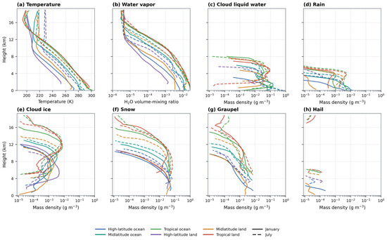
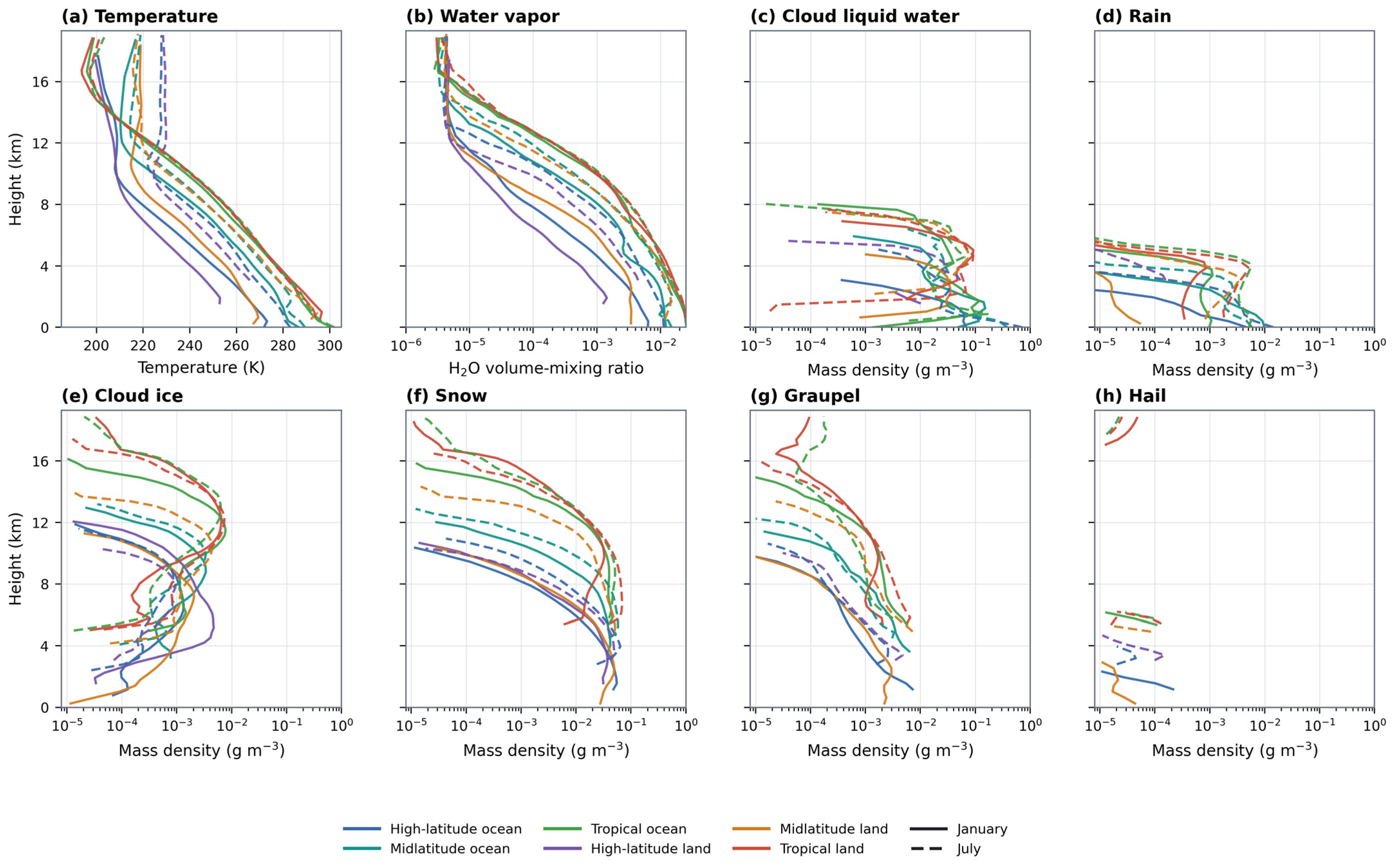
Figure 10 summarizes the 12 representative composites, whose total frozen-hydrometeor paths range from 0.157 to 0.430 kg m⁻². Snow is the largest frozen-path component in every composite, while cloud ice, graupel, and hail vary across latitude, surface type, and month. The 12 composites provide the cross-scene evaluation, while the two 100-profile ensembles test profile-level and seasonal consistency.

Figure 10. WRF-statistical representative composite profiles for the twelve evaluation scenes. The panels show temperature, water vapor, and the mass densities of cloud liquid water, rain, cloud ice, snow, graupel, and hail. Color identifies the six latitude–surface classes, and line style distinguishes the January and July scenes. Temperature and water vapor are taken from scene-specific WRF medoid profiles, while hydrometeor amounts and normalized vertical structures are derived from robust statistics of the corresponding cloudy populations.

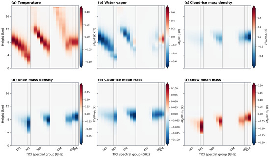
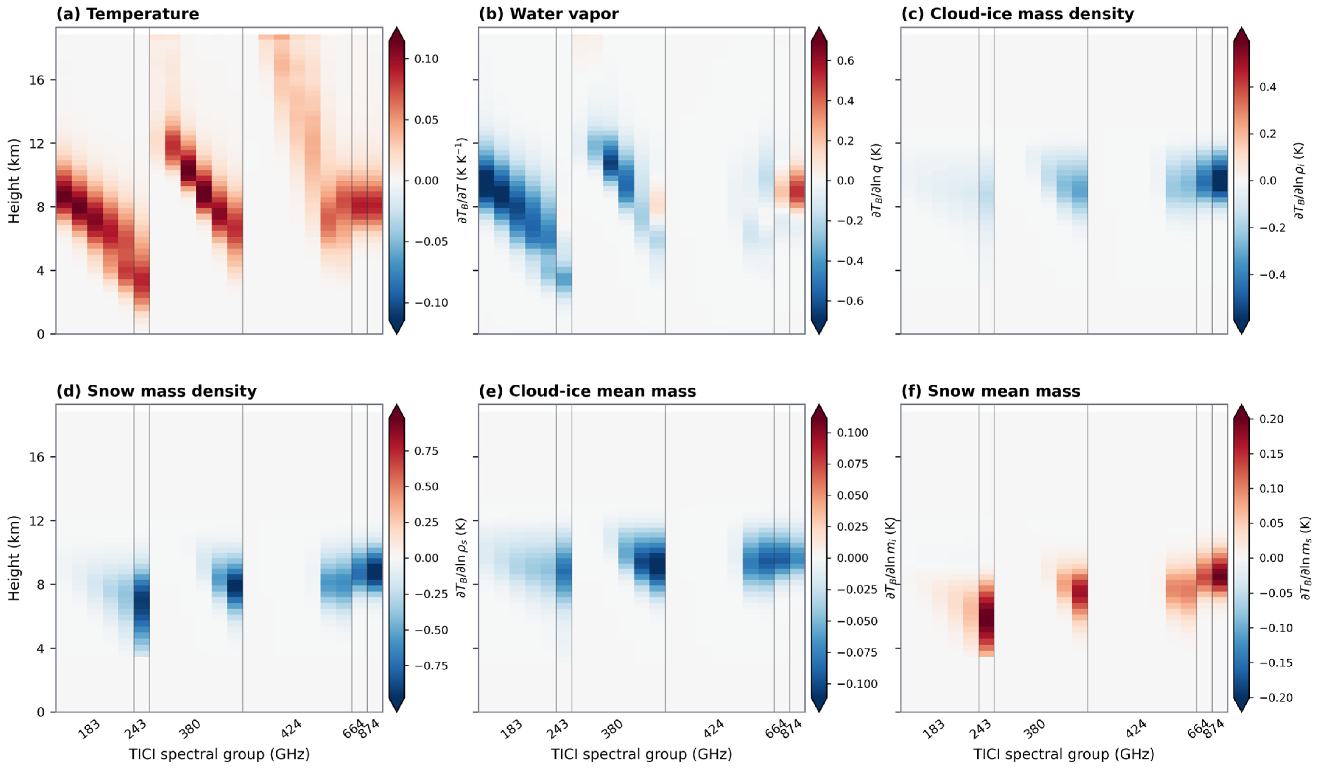
Figure 11 shows local Jacobians for the January midlatitude-ocean composite. Their magnitude and sign vary because perturbations alter emission, attenuation, and scattering. Negative water-vapor Jacobians at some 380 GHz observations reflect greater opacity shifting sensitivity toward higher, colder layers. These derivatives apply to the adopted linearization state rather than implying globally monotonic responses.

Figure 11. Local finite-difference Jacobians for the January midlatitude-ocean scene. The panels show temperature, water vapor, cloud-ice and snow mass densities, and the corresponding mean-particle-mass variables for the 21 scalar TICI observations.

4.3.2. Overall Information Content of the Complete Scalar TICI Observation Vector

The principal comparison evaluates TICI21 against ICI11 using paired simulations with identical states, surfaces, priors, forward models, and numerical settings. Differences are TICI21 minus ICI11. Because the vectors contain 21 and 11 scalar observations, the complete-system comparison does not measure information efficiency per observation.

Under channel-specific NEDTs (Table 6), TICI21 increases the 12-scene mean total DFS from 5.676 to 6.587. Temperature and water-vapor gains are 0.424 and 0.408, giving +0.831 for their combined group; frozen-hydrometeor DFS increases by 0.104. These differences are nonnegative in all 12 scenes, whereas liquid-hydrometeor DFS decreases by 0.025 on average.

Table 6. Mean DFS for the complete ICI11 and TICI21 configurations under channel-specific and uniform 1 K noise.

Evaluation Set and Noise Setting	State Group	ICI11 DFS	TICI21 DFS	$\mathsf{\Delta }$DFS
12 representative composites, channel-specific NEDT	Total	5.6761	6.5871	+0.9109
	Temperature	0.4348	0.8583	+0.4235
	Water vapor	0.9464	1.3541	+0.4077
	Temperature + water vapor	1.3812	2.2125	+0.8312
	Liquid hydrometeors	0.5310	0.5064	−0.0246
	Frozen hydrometeors	3.7639	3.8681	+0.1043
12 representative composites, uniform 1 K	Total	5.9744	7.2389	+1.2645
	Temperature	0.5348	1.3122	+0.7773
	Water vapor	0.8870	1.3617	+0.4747
	Temperature + water vapor	1.4218	2.6739	+1.2520
	Liquid hydrometeors	0.5185	0.4478	−0.0708
	Frozen hydrometeors	4.0341	4.1173	+0.0832
January + July midlatitude ocean, 200 WRF-derived profiles, uniform 1 K	Total	5.0596	6.3209	+1.2613
	Temperature	0.7302	1.7862	+1.0559
	Water vapor	1.6729	1.8098	+0.1369
	Temperature + water vapor	2.4031	3.5959	+1.1928
	Liquid hydrometeors	0.2144	0.2063	−0.0081
	Frozen hydrometeors	2.4421	2.5187	+0.0766

Note: Differences were calculated from unrounded values; independently rounded entries may therefore differ slightly from the displayed difference.

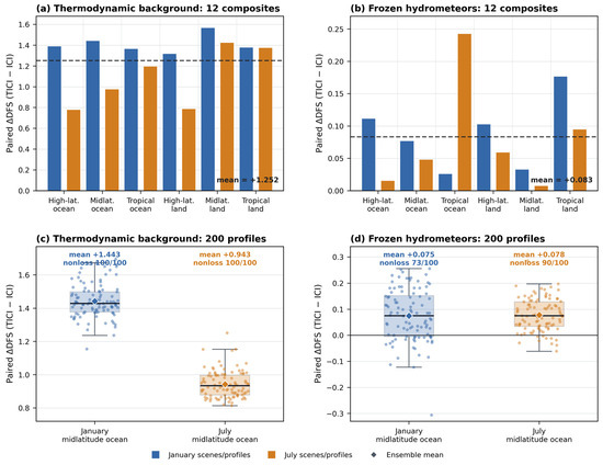
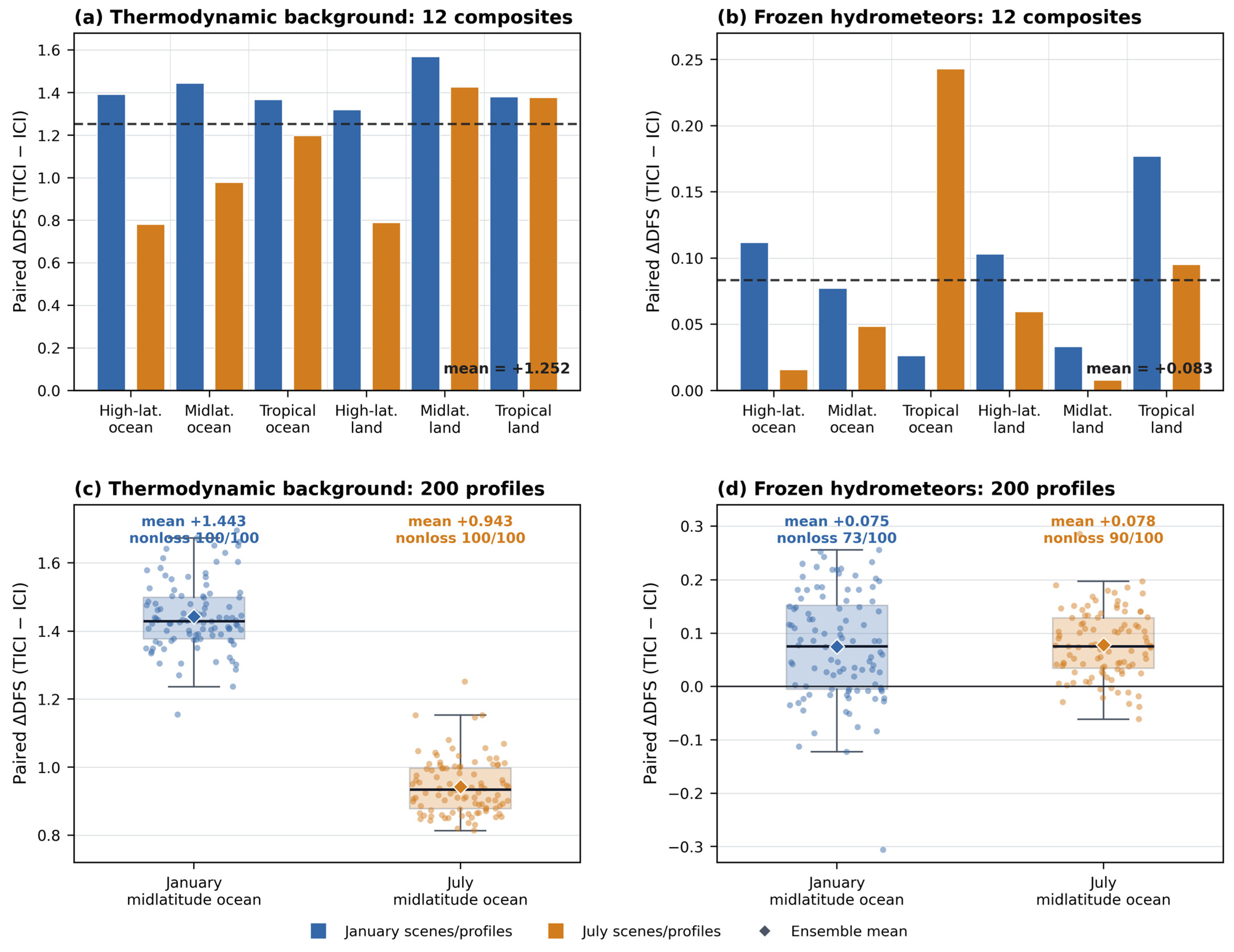
Under uniform 1 K noise, TICI21 increases the 12-scene mean total, temperature-plus-water-vapor, and frozen-hydrometeor DFS by 1.264, 1.252, and 0.083, respectively. These differences are nonnegative in every scene; the liquid-hydrometeor difference remains negative.

The 200-profile evaluation shows the same mean behavior (Figure 12): total, temperature-plus-water-vapor, and frozen-hydrometeor differences are +1.261, +1.193, and +0.077. Total and combined thermodynamic differences are nonnegative for all profiles, while frozen-hydrometeor differences are nonnegative for 163 profiles (81.5%) and remain positive in both monthly means.

Figure 12. Paired TICI21-minus-ICI11 DFS differences under uniform independent 1 K noise. Panels (a,b) show the temperature-plus-water-vapor and frozen-hydrometeor differences for the twelve WRF-statistical representative composites, grouped by latitude–surface class and month. Panels (c,d) show the corresponding distributions across the 100 January and 100 July midlatitude-ocean WRF-derived profiles. Diamonds identify ensemble means, and the annotations report the mean difference and number of profiles with nonnegative differences. The dashed horizontal lines in panels (a,b) indicate the corresponding mean values across the twelve composites.

4.3.3. Hydrometeor-Resolved Information Content

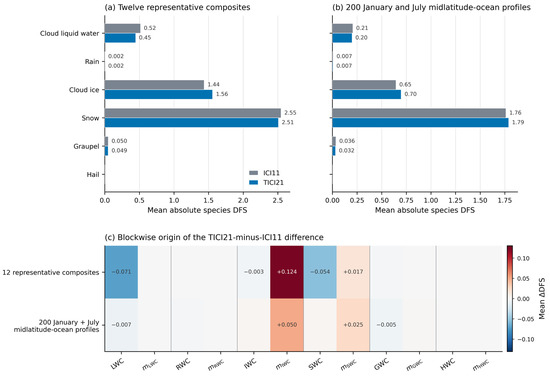
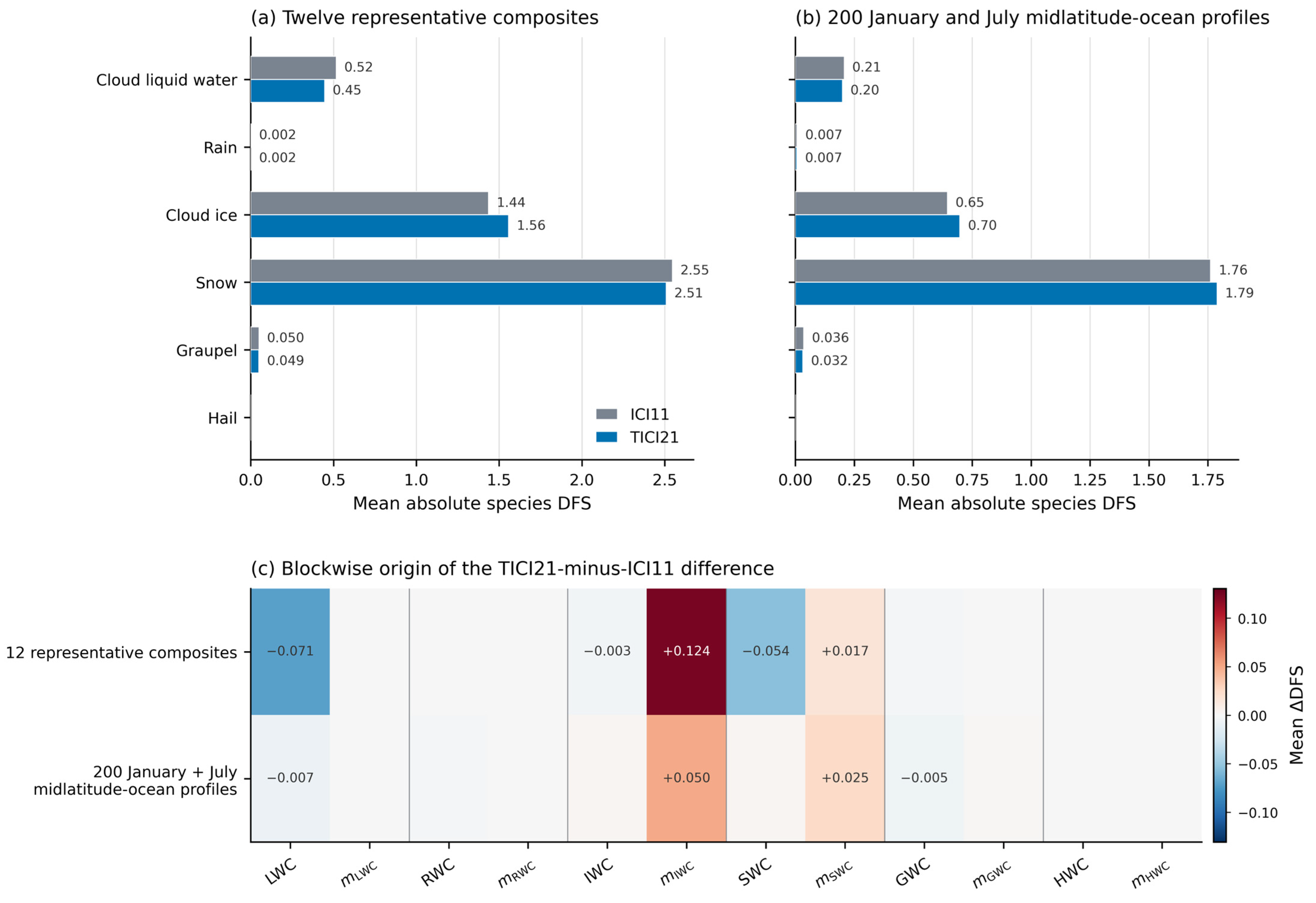
Table 7 and Figure 13 partition hydrometeor DFS by species and by mass-density and mean-particle-mass blocks. Across the 12 composites, cloud-ice DFS is 1.437 for ICI11 and 1.558 for TICI21, while snow DFS is 2.547 and 2.510, respectively.

Table 7. Species-resolved hydrometeor DFS for ICI11 and TICI21 under uniform independent 1 K noise.

Hydrometeor Species or Phase	12-Scene Mean: ICI11	12-Scene Mean: TICI21	$\mathsf{\Delta }$	200-Profile Mean: ICI11	200-Profile Mean: TICI21	$\mathsf{\Delta }$
Cloud liquid water	0.5167	0.4463	−0.0704	0.2070	0.1995	−0.0075
Rain	0.0018	0.0015	$\approx 0$	0.0073	0.0068	$\approx 0$
Liquid subtotal	0.5185	0.4478	−0.0708	0.2144	0.2063	−0.0081
Cloud ice	1.4370	1.5580	+0.1210	0.6452	0.6975	+0.0523
Snow	2.5470	2.5097	−0.0372	1.7614	1.7893	+0.0278
Graupel	0.0500	0.0495	$\approx 0$	0.0355	0.0320	−0.0036
Hail	$\approx 0$	$\approx 0$	$\approx 0$	$\approx 0$	$\approx 0$	$\approx 0$
Frozen subtotal	4.0341	4.1173	+0.0832	2.4421	2.5187	+0.0766

Figure 13. Hydrometeor-resolved DFS under uniform independent 1 K noise. Panels (a,b) compare the absolute ICI11 and TICI21 DFS of the six hydrometeor species for the twelve WRF-statistical representative composites and the 200 January and July midlatitude-ocean WRF-derived profiles, respectively. Panel (c) shows the corresponding TICI21-minus-ICI11 differences for all six mass-density and six mean-particle-mass state blocks. Positive values indicate larger DFS for TICI21. Numerical labels are omitted below 0.001 DFS in panels (a,b) and below 0.003 DFS in panel (c).

For the 12 composites, the +0.0832 frozen-hydrometeor difference arises mainly from mean-particle-mass states. Frozen mass-density blocks sum to −0.0593 DFS, whereas mean-particle-mass blocks sum to +0.1425; the largest term is the cloud-ice mean-particle-mass gain (+0.1244). Thus, the aggregate gain does not indicate improvement in every frozen state variable.

The 200 profiles show the same partition: frozen mass-density DFS is nearly unchanged (−0.0005), while mean-particle-mass DFS increases by +0.0771, reproducing the +0.0766 frozen-hydrometeor difference. Cloud-ice and snow mean-particle-mass differences are positive in both monthly ensembles, whereas their mass-density differences vary by month.

4.3.4. Band-Level and Channel-Level Contributions

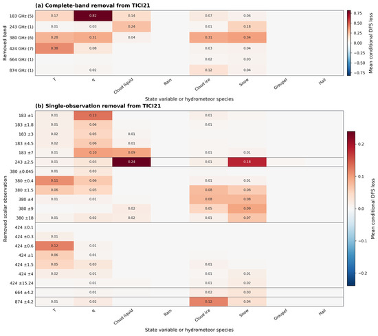
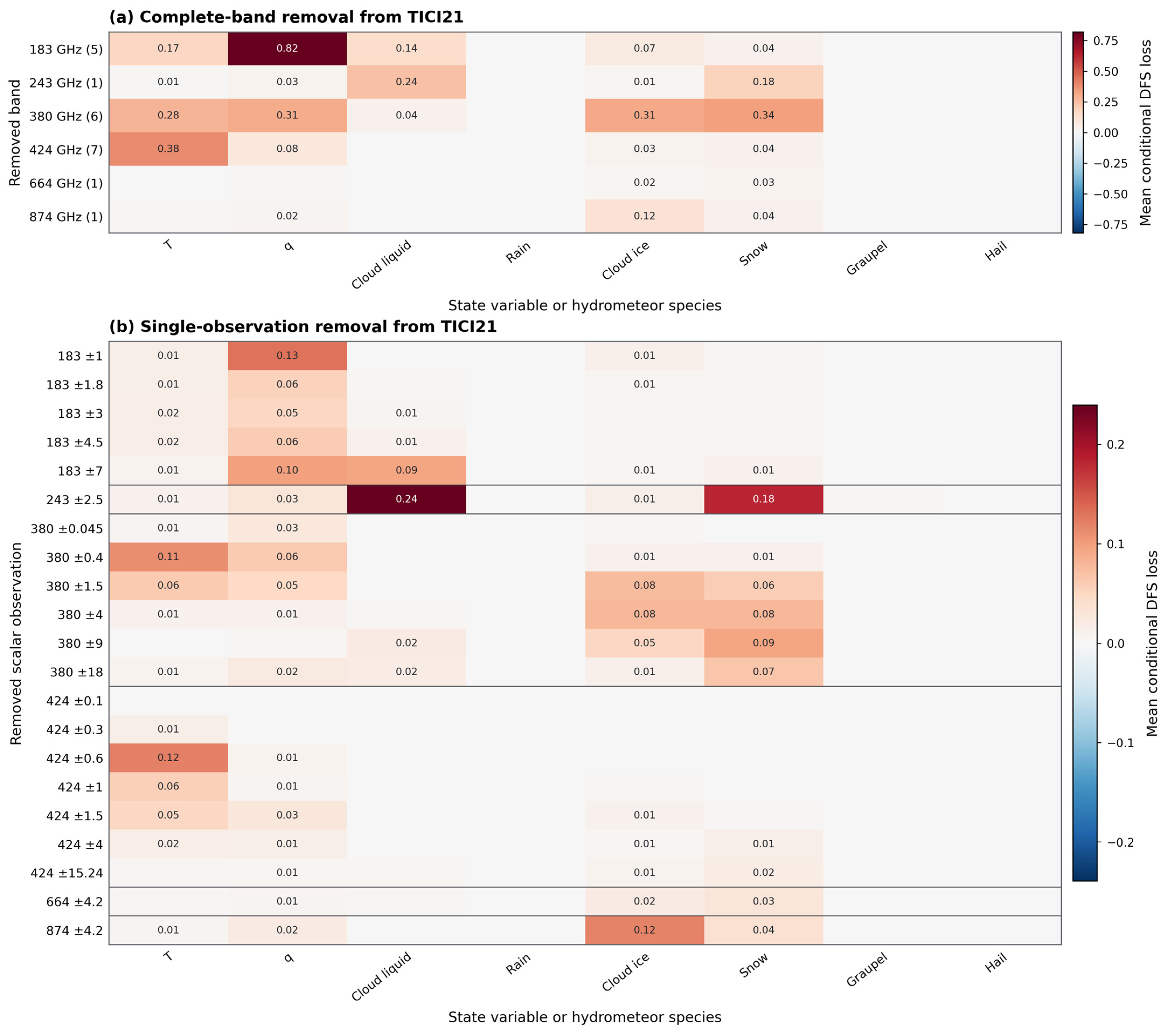
Band removal shows overlapping spectral roles (Figure 14a). Removing 183 GHz causes the largest water-vapor loss (0.819 DFS), removing 424 GHz causes the largest temperature loss (0.385), and removing 380 GHz causes losses in temperature (0.281), water vapor (0.307), and frozen hydrometeors (0.652). Frozen-hydrometeor losses are also 0.200 at 243 GHz and 0.157 at 874 GHz, the latter mainly from mean-particle-mass states. The 424 GHz frozen loss is smaller but nonzero (0.065). Removing 183 and 243 GHz also reduces cloud-liquid-water DFS, while rain DFS remains negligible.

Figure 14. Conditional DFS losses caused by removing observations from TICI21, averaged over the twelve WRF-statistical representative composites under uniform independent 1 K noise. Panel (a) removes each complete TICI spectral band, and panel (b) removes each of the 21 scalar observations individually. Columns show temperature, water vapor, and the combined mass-density-plus-mean-particle-mass DFS of each hydrometeor species. Positive values indicate information lost after removal. The values are conditional on the retained observations and the full scene-specific prior and are not additive across bands or channels. Numerical labels are omitted for values with absolute magnitude below 0.01 DFS in panel (a) and 0.005 DFS in panel (b).

The 424 GHz band is not exclusively a temperature band. Removing the ±0.6 GHz observation reduces temperature DFS by 0.121 but frozen-hydrometeor DFS by less than 0.001; removing ±4 and ±15.24 GHz reduces frozen-hydrometeor DFS by 0.019 and 0.026, mainly through cloud-ice and snow blocks (Figure 14b).

The largest single-observation frozen-hydrometeor losses occur at 243.25 ± 2.5 GHz (0.200), 380.1974 ± 4 GHz (0.161), 874 ± 4.2 GHz (0.157), and the ±9 and ±1.5 GHz observations near 380 GHz (0.146 and 0.136). Thus, middle-to-outer 380 GHz observations and 874 GHz provide the strongest TICI-specific frozen-hydrometeor increments.

The spectrally representative 325-to-380, 448-to-424, and joint replacements increase 12-scene mean temperature-plus-water-vapor DFS by 0.290, 0.070, and 0.444, respectively (Table 8). The contribution-informed joint subset increases the 12-scene mean temperature-plus-water-vapor and total DFS by 0.733 and 0.241, while frozen-hydrometeor DFS decreases by 0.371. Across the 200 profiles, the corresponding temperature-plus-water-vapor and total differences are +0.747 and +0.507 and are nonnegative for every profile; the mean frozen-hydrometeor difference remains negative at −0.221. The controlled tests show that frequency placement contributes to the thermodynamic gain, but the selected 380 and 424 GHz substitutions do not reproduce all ICI11 frozen-hydrometeor information. The complete TICI21 vector additionally includes the full multi-band sampling and 874 GHz.

Table 8. Twelve-scene mean DFS differences for controlled 11-observation replacements under uniform independent 1 K noise.

Controlled Replacement	$\mathsf{\Delta }\mathit{T}$ DFS	$\mathsf{\Delta }\mathit{q}$ DFS	$\mathsf{\Delta }\left(\mathit{T}+\mathit{q}\right)$ DFS	$\mathsf{\Delta }$frozen DFS	$\mathsf{\Delta }$total DFS
325 → 380 GHz	+0.1620	+0.1285	+0.2905	−0.1543	+0.0379
448 → 424 GHz	+0.1517	−0.0819	+0.0699	−0.4288	−0.3699
325 + 448 → 380 + 424 GHz	+0.3218	+0.1222	+0.4440	−0.5634	−0.2324
325 + 448 → 380 + 424 GHz, contribution-informed subset	+0.5791	+0.1540	+0.7331	−0.3712	+0.2412

Note: Differences were calculated from unrounded values; independently rounded entries may therefore differ slightly from the displayed difference. → means frequency-band replacement.

Overall, TICI21 provides more thermodynamic information while retaining a small positive mean frozen-hydrometeor difference that is concentrated in mean-particle-mass states. These estimates are conditional on the January and July 2014 WRF populations, scene-specific OAS priors, state transformations, and local linearization states. Cloud ice is represented as spherical, and no cloud-ice-habit sensitivity test is included. This approximation may affect the absolute and species-resolved DFS estimates. Surface emissivity is fixed by surface type, while frequency-, polarization-, and scene-dependent variability is omitted. Because ${\mathit{S}}_{\epsilon }$ includes channel noise but not forward-model error and the analysis uses scalar Stokes-I observations, the absolute DFS may be optimistic and should not be interpreted as retrieval accuracy.

4.4. Conceptual TICI Payload Architecture and Engineering Considerations

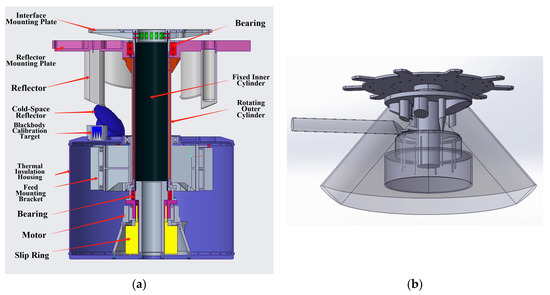
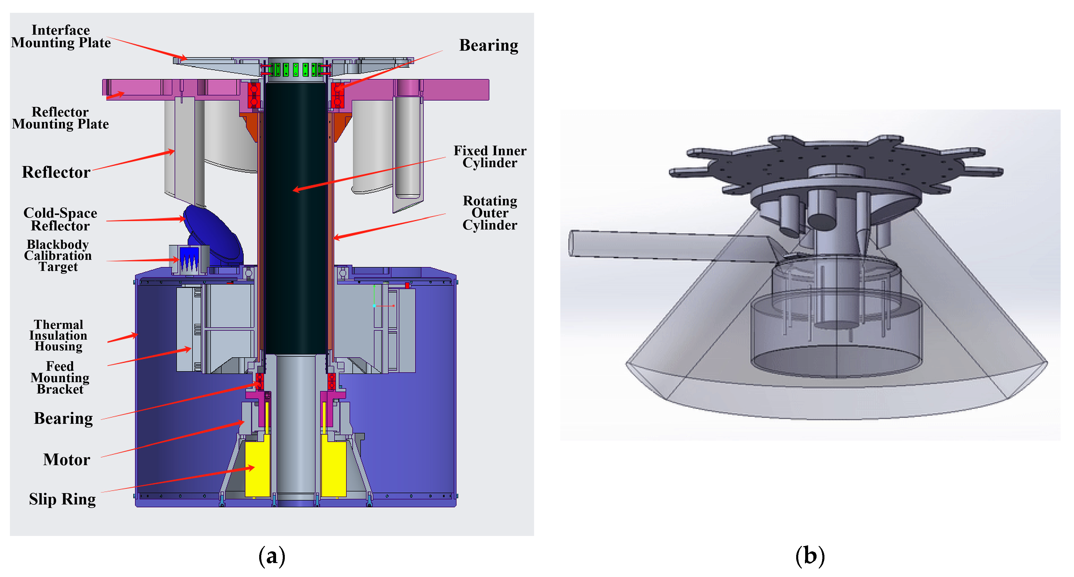
The conceptual TICI payload uses independent reflector/feed systems for six bands, totaling eight feeds and eight reflectors (Figure 15 and Table 9). The eight reflectors are uniformly distributed on a circular support disk. The 243 GHz feed uses an orthomode transducer for V/H separation; separate V- and H-polarized reflector/feed sets are used at 664 and 874 GHz. Receiver electronics are housed centrally, with cold-space and blackbody targets providing two-point calibration. The reflector and receiver/feed assemblies rotate together at a constant speed around a fixed central axis. The scanning period is 2 s, during which the satellite travels approximately 15 km along its orbit. This scanning configuration provides contiguous ground coverage.

Figure 15. Conceptual configuration of TICI: (a) arrangement of the reflector/feed, calibration, and rotating assemblies; and (b) conceptual mechanical arrangement of the reflector/feed assemblies and their schematic viewing cones. In panel (a), red arrows connect the labels to the corresponding components; colors are used to distinguish the structural components.

Table 9. Antenna polarization and implementation for TICI.

Assembly Group	Frequency (GHz)	Polarization	Reflector/Feed Assemblies
1	183	H	1
2	243	V + H	1 (OMT)
3	380	H	1
4	424	H	1
5	664	V + H	2
6	874	V + H	2

In subsequent data processing, observations from all channels can be geolocated and resampled to a common ground grid or common geographic coordinates.

Antenna simulations for all six bands yield approximately symmetric patterns and similar beam widths (Table 10), with main-beam efficiencies above 95%, sidelobes at or below −30 dB, and cross-polarization at or below −26 dB.

Table 10. Simulated TICI antenna performance.

Frequency (GHz)	Beam Width (°)	Main-Beam Efficiency	Cross-Polarization (dB)	Sidelobe (dB)
183	0.56	>97%	−26	−30
243	0.53	>96%	−27	−32
380	0.58	>96%	−29	−30
424	0.58	>97%	−29	−30
664	0.54	>95%	−32	−31
874	0.56	>95%	−33	−35

Table 11 reports single-beam nominal ground-projected dimensions derived from the simulated beamwidths under the assumed orbit and viewing geometry. The information-content analysis assumes collocated observations across the TICI channels, and detailed spatial and temporal co-registration requires further engineering design. The design assumes an approximately 820 km sun-synchronous orbit, 30 rpm conical scanning, a 53° incidence angle, and a ±60° scan range, producing a swath wider than 1700 km. The apertures in Table 11 target an approximately 16 km band-level spatial resolution. This design target is distinct from the reported major and minor dimensions of each elliptical ground-projected single-beam footprint, although the quantities are related through the simulated beamwidth and assumed viewing geometry.

Table 11. Antenna apertures, spatial resolutions, and pixel sizes for the six TICI frequency bands.

Frequency (GHz)	Antenna Aperture (cm)	Spatial Resolution (km)	Pixel Size (km)
183	23	16	12.4 × 21.7
243	17	16	12.7 × 21.1
380	11	16	12.5 × 20.8
424	10	16	12.5 × 20.7
664	6.3	16	12.5 × 20.8
874	4.8	16	12.5 × 20.7

The conceptual architecture does not prescribe a receiver implementation. Previous work by members of our group developed the TALIS receiver using four room-temperature superheterodyne radiometers centered at 118, 190, 240, and 640 GHz, together with four fast Fourier transform spectrometers, and reported preliminary hot- and cold-target tests [56]. This work provides a relevant hardware research basis for TICI. Receiver readiness, 1/f noise, and calibration stability, especially at the highest frequencies, require further assessment; the adopted NEDTs remain design assumptions.

Quantitative payload mass, power consumption, and volume have not yet been determined in the present conceptual study. The angular momentum associated with the synchronous rotation of the eight reflector/feed assemblies, the required compensation scheme, and the resulting effects on platform attitude stability and pointing accuracy also require further engineering analysis.

Future mission studies should assess the incremental value of the 380 and 424 GHz bands alongside dedicated temperature and humidity sounders on other payloads.

5. Conclusions

This study evaluates a candidate six-band TICI configuration for next-generation Fengyun polar-orbiting satellites. The 183 and 380 GHz bands constrain water vapor; 424 GHz primarily constrains temperature while its outer wings retain cloud-ice and snow sensitivity; and the 243, 664, and 874 GHz windows provide complementary ice-scattering sensitivity. The configuration is therefore a candidate multi-band design, not an optimized or universally superior channel set.

The information-content results are conditional on the 2014 WRF populations, scene-specific OAS priors, adopted state transformations, fixed surface emissivities, diagonal channel noise, and scalar Stokes-I observations. Spherical cloud ice was applied consistently to TICI21 and ICI11 but was not tested against nonspherical habits. Because surface variability and other forward-model errors are absent from ${\mathit{S}}_{\epsilon }$, absolute and species-resolved DFS may be optimistic.

Under uniform 1 K noise, TICI21 retains a small positive mean frozen-hydrometeor difference, driven by mean-particle-mass rather than frozen mass-density states. The 380 GHz band contributes to thermodynamic and frozen information, the 424 GHz outer wings retain cloud-ice and snow information, and 874 GHz adds a high-frequency frozen-hydrometeor constraint. Equal-dimensional tests confirm that frequency placement contributes to the thermodynamic gain, but the selected 380 and 424 GHz substitutions do not fully reproduce ICI11 frozen-hydrometeor information.

The conceptual payload comprises eight reflector/feed assemblies uniformly distributed on a circular support disk and rotating synchronously about a fixed central axis with a 2 s scan period. During one rotation, the satellite travels approximately 15 km, providing contiguous ground coverage. Observations from all channels can subsequently be geolocated and resampled to a common ground grid or geographic coordinates. Antenna simulations yield main-beam efficiencies above 95%, with sidelobes at or below −30 dB, cross-polarization at or below −26 dB, and an approximately 16 km spatial-resolution target across the six bands. Quantitative payload mass, power consumption, and volume, as well as scan-induced angular momentum, compensation requirements, platform pointing stability, channel co-registration, receiver implementation, calibration, and end-to-end retrieval performance, require further engineering assessment.

References

- Costa, A.; Meyer, J.; Afchine, A.; Luebke, A.; Günther, G.; Dorsey, J.R.; Gallagher, M.W.; Ehrlich, A.; Wendisch, M.; Baumgardner, D.; et al. Classification of Arctic, Midlatitude and Tropical Clouds in the Mixed-Phase Temperature Regime. Atmos. Chem. Phys. 2017, 17, 12219–12238. [Google Scholar] [CrossRef] [Scilit]
- Wylie, D.P.; Menzel, W.P.; Woolf, H.M.; Strabala, K.I. Four Years of Global Cirrus Cloud Statistics Using HIRS. J. Clim. 1994, 7, 1972–1986. [Google Scholar] [CrossRef] [Scilit]
- Chen, Y.; Liou, K.N.; Gu, Y. An Efficient Diffusion Approximation for 3D Radiative Transfer Parameterization: Application to Cloudy Atmospheres. J. Quant. Spectrosc. Radiat. Transf. 2005, 92, 189–200. [Google Scholar] [CrossRef] [Scilit]
- Houze, R.A., Jr. Cloud Dynamics, 2nd ed.; Academic Press: Oxford, UK, 2014; Volume 104. [Google Scholar]
- Buehler, S.A.; Jiménez, C.; Evans, K.F.; Eriksson, P.; Rydberg, B.; Heymsfield, A.J.; Stubenrauch, C.J.; Lohmann, U.; Emde, C.; John, V.O.; et al. A Concept for a Satellite Mission to Measure Cloud Ice Water Path, Ice Particle Size, and Cloud Altitude. Q. J. R. Meteorol. Soc. 2007, 133, 109–128. [Google Scholar] [CrossRef] [Scilit]
- Stephens, G.L.; Vane, D.G.; Tanelli, S.; Im, E.; Durden, S.; Rokey, M.; Reinke, D.; Partain, P.; Mace, G.G.; Austin, R.; et al. CloudSat Mission: Performance and Early Science after the First Year of Operation. J. Geophys. Res. Atmos. 2008, 113, D00A18. [Google Scholar] [CrossRef] [Scilit]
- Winker, D.M.; Vaughan, M.A.; Omar, A.; Hu, Y.; Powell, K.A.; Liu, Z.; Hunt, W.H.; Young, S.A. Overview of the CALIPSO Mission and CALIOP Data Processing Algorithms. J. Atmos. Ocean. Technol. 2009, 26, 2310–2323. [Google Scholar] [CrossRef] [Scilit]
- Deng, M.; Mace, G.G.; Wang, Z.; Berry, E. CloudSat 2C-ICE Product Update with a New Ze Parameterization in Lidar-only Region. J. Geophys. Res. Atmos. 2015, 120, 12198–12208. [Google Scholar] [CrossRef] [Scilit] [PubMed]
- Wehr, T.; Kubota, T.; Tzeremes, G.; Wallace, K.; Nakatsuka, H.; Ohno, Y.; Koopman, R.; Rusli, S.; Kikuchi, M.; Eisinger, M.; et al. The EarthCARE Mission–Science and System Overview. Atmos. Meas. Tech. 2023, 16, 3581–3608. [Google Scholar] [CrossRef] [Scilit]
- Gong, J.; Wu, D.L. Microphysical Properties of Frozen Particles Inferred from Global Precipitation Measurement (GPM) Microwave Imager (GMI) Polarimetric Measurements. Atmos. Chem. Phys. 2017, 17, 2741–2757. [Google Scholar] [CrossRef] [Scilit] [PubMed]
- Defer, E.; Galligani, V.S.; Prigent, C.; Jiménez, C. First Observations of Polarized Scattering over Ice Clouds at Close-to-Millimeter Wavelengths (157 GHz) with MADRAS on Board the Megha-Tropiques Mission. J. Geophys. Res. Atmos. 2014, 119, 12301–12316. [Google Scholar] [CrossRef] [Scilit]
- Zou, X.; Chen, X.; Weng, F. Polarization Signature from the FengYun-3 Microwave Humidity Sounder. Front. Earth Sci. 2014, 8, 625–633. [Google Scholar] [CrossRef] [Scilit]
- Wu, D.L.; Gong, J.; Deal, W.R.; Gaines, W.; Cooke, C.M.; De Amici, G.; Pantina, P.; Liu, Y.; Yang, P.; Eriksson, P.; et al. Remote Sensing of Ice Cloud Properties with Millimeter and Submillimeter-Wave Polarimetry. IEEE J. Microw. 2024, 4, 847–857. [Google Scholar] [CrossRef] [Scilit]
- Evans, K.F.; Stephens, G.L. Microwave Radiative Transfer through Clouds Composed of Realistically Shaped Ice Crystals. Part II. Remote Sensing of Ice Clouds. J. Atmos. Sci. 1995, 52, 2058–2072. [Google Scholar] [CrossRef] [Scilit]
- Evans, K.F.; Wang, J.R.; O’C Starr, D.; Heymsfield, G.; Li, L.; Tian, L.; Lawson, R.P.; Heymsfield, A.J.; Bansemer, A. Ice Hydrometeor Profile Retrieval Algorithm for High-Frequency Microwave Radiometers: Application to the CoSSIR Instrument during TC4. Atmos. Meas. Tech. 2012, 5, 2277–2306. [Google Scholar] [CrossRef] [Scilit]
- Fox, S.; Lee, C.; Moyna, B.; Philipp, M.; Rule, I.; Rogers, S.; King, R.; Oldfield, M.; Rea, S.; Henry, M.; et al. ISMAR: An Airborne Submillimetre Radiometer. Atmos. Meas. Tech. 2017, 10, 477–490. [Google Scholar] [CrossRef] [Scilit]
- Evans, K.F.; Wang, J.R.; Racette, P.E.; Heymsfield, G.; Li, L. Ice Cloud Retrievals and Analysis with the Compact Scanning Submillimeter Imaging Radiometer and the Cloud Radar System during CRYSTAL FACE. J. Appl. Meteorol. 2005, 44, 839–859. [Google Scholar] [CrossRef] [Scilit][Green Version]
- Brath, M.; Fox, S.; Eriksson, P.; Harlow, R.C.; Burgdorf, M.; Buehler, S.A. Retrieval of an Ice Water Path over the Ocean from ISMAR and MARSS Millimeter and Submillimeter Brightness Temperatures. Atmos. Meas. Tech. 2018, 11, 611–632. [Google Scholar] [CrossRef] [Scilit]
- Wu, D.L.; Piepmeier, J.R.; Esper, J.; Ehsan, N.; Racette, P.E.; Johnson, T.E.; Abresch, B.S.; Bryerton, E. IceCube: Submm-Wave Technology Development for Future Science on a CubeSat. In The Nanosatellite Revolution: 25 Years and Counting; SPIE: Bellingham, WA, USA, 2019. [Google Scholar]
- Gong, J.; Wu, D.L.; Eriksson, P. The First Global 883 GHz Cloud Ice Survey: IceCube Level 1 Data Calibration, Processing and Analysis. Earth Syst. Sci. Data 2021, 13, 5369–5387. [Google Scholar] [CrossRef] [Scilit]
- Eriksson, P.; Emrich, A.; Kempe, K.; Riesbeck, J.; Aljarosha, A.; Auriacombe, O.; Kugelberg, J.; Hekma, E.; Albers, R.; Murk, A.; et al. The Arctic Weather Satellite Radiometer. Atmos. Meas. Tech. 2025, 18, 4709–4729. [Google Scholar] [CrossRef] [Scilit]
- Eriksson, P.; Rydberg, B.; Mattioli, V.; Thoss, A.; Accadia, C.; Klein, U.; Buehler, S.A. Towards an Operational Ice Cloud Imager (ICI) Retrieval Product. Atmos. Meas. Tech. 2020, 13, 53–71. [Google Scholar] [CrossRef] [Scilit]
- Guan, M.; Wang, J.; Zhao, X.; Qin, D.; Fan, C.; Xian, D.; Liu, C. Progress and Achievements of Fengyun Meteorological Satellite Program since 2022. Chin. J. Space Sci. 2024, 44, 712–721. [Google Scholar] [CrossRef] [Scilit]
- China Meteorological Administration. CMA Updates Since CGMS-53 and Report on the Medium to Long-Term Future Plans on Earth Observation; Working Paper CGMS-54-CMA-WP-16-p; Coordination Group for Meteorological Satellites: Darmstadt, Germany, 2 June 2026; Available online: https://www.cgms-info.org/Agendas/GetWpFile.ashx?aid=d79a544f-c6be-4c1c-bac4-e3790000f568&wid=eb439a26-890b-455f-90f9-bf539c3da224 (accessed on 12 September 2026).
- Chen, K.; Chen, Y.; Suo, Z.; Han, W. Hybrid Observing System Simulation Experiment for the FY-4 Geostationary Orbit Microwave Satellite Based on CMA-GFS. IEEE Trans. Geosci. Remote Sens. 2026, 64, 4100721. [Google Scholar] [CrossRef] [Scilit]
- Buehler, S.A.; Larsson, R.; Lemke, O.; Pfreundschuh, S.; Brath, M.; Adams, I.; Fox, S.; Roemer, F.E.; Czarnecki, P.; Eriksson, P. The Atmospheric Radiative Transfer Simulator ARTS, Version 2.6—Deep Python Integration. J. Quant. Spectrosc. Radiat. Transf. 2025, 341, 109443. [Google Scholar] [CrossRef] [Scilit]
- Fox, S. An Evaluation of Radiative Transfer Simulations of Cloudy Scenes from a Numerical Weather Prediction Model at Sub-Millimetre Frequencies Using Airborne Observations. Remote Sens. 2020, 12, 2758. [Google Scholar] [CrossRef] [Scilit]
- Fox, S.; Mattioli, V.; Turner, E.; Vance, A.; Cimini, D.; Gallucci, D. An Evaluation of Atmospheric Absorption Models at Millimetre and Sub-Millimetre Wavelengths Using Airborne Observations. Atmos. Meas. Tech. 2024, 17, 4957–4978. [Google Scholar] [CrossRef] [Scilit]
- Larosa, S.; Cimini, D.; Gallucci, D.; Nilo, S.T.; Romano, F. PyRTlib: An Educational Python-Based Library for Non-Scattering Atmospheric Microwave Radiative Transfer Computations. Geosci. Model Dev. 2024, 17, 2053–2076. [Google Scholar] [CrossRef] [Scilit]
- Perrin, A.; Puzzarini, C.; Colmont, J.-M.; Verdes, C.; Wlodarczak, G.; Cazzoli, G.; Buehler, S.; Flaud, J.-M.; Demaison, J. Molecular Line Parameters for the MASTER (Millimeter Wave Acquisitions for Stratosphere/Troposphere Exchange Research) Database. J. Atmos. Chem. 2005, 51, 161–205. [Google Scholar] [CrossRef] [Scilit][Green Version]
- Eriksson, P.; Ekelund, R.; Mendrok, J.; Brath, M.; Lemke, O.; Buehler, S.A. A General Database of Hydrometeor Single Scattering Properties at Microwave and Sub-Millimetre Wavelengths. Earth Syst. Sci. Data 2018, 10, 1301–1326. [Google Scholar] [CrossRef] [Scilit]
- Buras, R.; Dowling, T.; Emde, C. New Secondary-Scattering Correction in DISORT with Increased Efficiency for Forward Scattering. J. Quant. Spectrosc. Radiat. Transf. 2011, 112, 2028–2034. [Google Scholar] [CrossRef] [Scilit]
- Buehler, S.A.; Defer, E.; Evans, F.; Eliasson, S.; Mendrok, J.; Eriksson, P.; Lee, C.; Jiménez, C.; Prigent, C.; Crewell, S.; et al. Observing Ice Clouds in the Submillimeter Spectral Range: The CloudIce Mission Proposal for ESA’s Earth Explorer 8. Atmos. Meas. Tech. 2012, 5, 1529–1549. [Google Scholar] [CrossRef] [Scilit]
- Birman, C.; Mahfouf, J.-F.; Milz, M.; Mendrok, J.; Buehler, S.A.; Brath, M. Information Content on Hydrometeors from Millimeter and Sub-Millimeter Wavelengths. Tellus A Dyn. Meteorol. Oceanogr. 2017, 69, 1271562. [Google Scholar] [CrossRef] [Scilit]
- Skamarock, W.C.; Klemp, J.B.; Dudhia, J.; Gill, D.O.; Liu, Z.; Berner, J.; Wang, W.; Powers, J.G.; Duda, M.G.; Barker, D.M.; et al. A Description of the Advanced Research WRF Model Version 4; NCAR Technical Note NCAR/TN-556+STR; National Center for Atmospheric Research: Boulder, CO, USA, 2019; p. 145. [Google Scholar] [CrossRef]
- Anderson, G.P.; Clough, S.A.; Kneizys, F.X.; Chetwynd, J.H.; Shettle, E.P. AFGL Atmospheric Constituent Profiles (0–120 km); Technical Report AFGL-TR-86-0110; Air Force Geophysics Laboratory: Hanscom AFB, MA, USA, 1986. [Google Scholar]
- Hersbach, H.; Bell, B.; Berrisford, P.; Hirahara, S.; Horányi, A.; Muñoz-Sabater, J.; Nicolas, J.; Peubey, C.; Radu, R.; Schepers, D.; et al. The ERA5 Global Reanalysis. Q. J. R. Meteorol. Soc. 2020, 146, 1999–2049. [Google Scholar] [CrossRef] [Scilit]
- Brath, M.; Ekelund, R.; Eriksson, P.; Lemke, O.; Buehler, S.A. Microwave and Submillimeter Wave Scattering of Oriented Ice Particles. Atmos. Meas. Tech. 2020, 13, 2309–2333. [Google Scholar] [CrossRef] [Scilit]
- Bergada, M.; Labriola, M.; Gonzalez, R.; Palacios, M.A.; Marote, D.; Andres, A.; Garcia, J.L.; Sanchez-Pascuala, D.; Ordonez, L.; Rodriguez, M.; et al. The Ice Cloud Imager (ICI) Preliminary Design and Performance. In Proceedings of the 2016 14th Specialist Meeting on Microwave Radiometry and Remote Sensing of the Environment (MicroRad), Espoo, Finland, 11–14 April 2016; pp. 27–31. [Google Scholar] [CrossRef] [Scilit]
- Spencer, R.W.; Goodman, H.M.; Hood, R.E. Precipitation Retrieval over Land and Ocean with the SSM/I: Identification and Characteristics of the Scattering Signal. J. Atmos. Ocean. Technol. 1989, 6, 254–273. [Google Scholar] [CrossRef] [Scilit]
- Prigent, C.; Defer, E.; Pardo, J.R.; Pearl, C.; Rossow, W.B.; Pinty, J.-P. Relations of Polarized Scattering Signatures Observed by the TRMM Microwave Instrument with Electrical Processes in Cloud Systems. Geophys. Res. Lett. 2005, 32, L04810. [Google Scholar] [CrossRef] [Scilit]
- Zhao, L.; Weng, F. Retrieval of Ice Cloud Parameters Using the Advanced Microwave Sounding Unit. J. Appl. Meteorol. 2002, 41, 384–395. [Google Scholar] [CrossRef] [Scilit] [PubMed]
- Wang, Y.; Fu, Y.; Fang, X.; Zhang, Y. Estimating Ice Water Path in Tropical Cyclones with Multispectral Microwave Data From the FY-3B Satellite. IEEE Trans. Geosci. Remote Sens. 2014, 52, 5548–5557. [Google Scholar] [CrossRef] [Scilit]
- Wang, W.; Xu, J.; Letu, H.; Zhang, L.; Wang, Z.; Shi, J. A New Deep-Learning-Based Framework for Ice Water Path Retrieval From Microwave Humidity Sounder-II Aboard FengYun-3D Satellite. IEEE Trans. Geosci. Remote Sens. 2024, 62, 4101714. [Google Scholar] [CrossRef] [Scilit]
- Evans, K.F.; Walter, S.J.; Heymsfield, A.J.; McFarquhar, G.M. Submillimeter-Wave Cloud Ice Radiometer: Simulations of Retrieval Algorithm Performance. J. Geophys. Res. Atmos. 2002, 107, AAC 2-1–AAC 2-21. [Google Scholar] [CrossRef] [Scilit]
- Rodgers, C.D. Inverse Methods for Atmospheric Sounding: Theory and Practice; World Scientific: Singapore, 2000; Volume 2, ISBN 981-02-2740-X. [Google Scholar] [CrossRef]
- Iacono, M.J.; Delamere, J.S.; Mlawer, E.J.; Shephard, M.W.; Clough, S.A.; Collins, W.D. Radiative Forcing by Long-lived Greenhouse Gases: Calculations with the AER Radiative Transfer Models. J. Geophys. Res. Atmos. 2008, 113, D13103. [Google Scholar] [CrossRef] [Scilit]
- Hong, S.-Y.; Noh, Y.; Dudhia, J. A New Vertical Diffusion Package with an Explicit Treatment of Entrainment Processes. Mon. Weather Rev. 2006, 134, 2318–2341. [Google Scholar] [CrossRef] [Scilit]
- Milbrandt, J.A.; Yau, M.K. A Multimoment Bulk Microphysics Parameterization. Part I: Analysis of the Role of the Spectral Shape Parameter. J. Atmos. Sci. 2005, 62, 3051–3064. [Google Scholar] [CrossRef] [Scilit]
- Milbrandt, J.A.; Yau, M.K. A Multimoment Bulk Microphysics Parameterization. Part II: A Proposed Three-Moment Closure and Scheme Description. J. Atmos. Sci. 2005, 62, 3065–3081. [Google Scholar] [CrossRef] [Scilit]
- Kain, J.S.; Fritsch, J.M. Convective Parameterization for Mesoscale Models: The Kain-Fritsch Scheme. In The Representation of Cumulus Convection in Numerical Models; Emanuel, K.A., Raymond, D.J., Eds.; American Meteorological Society: Boston, MA, USA, 1993; pp. 165–170. ISBN 978-1-935704-13-3. [Google Scholar] [CrossRef] [Scilit]
- Eriksson, P. Analysis and Comparison of Two Linear Regularization Methods for Passive Atmospheric Observations. J. Geophys. Res. Atmos. 2000, 105, 18157–18167. [Google Scholar] [CrossRef] [Scilit]
- Eriksson, P.; Jiménez, C.; Buehler, S.A. Qpack, a General Tool for Instrument Simulation and Retrieval Work. J. Quant. Spectrosc. Radiat. Transf. 2005, 91, 47–64. [Google Scholar] [CrossRef] [Scilit]
- Chen, Y.; Wiesel, A.; Eldar, Y.C.; Hero, A.O. Shrinkage Algorithms for MMSE Covariance Estimation. IEEE Trans. Signal Process. 2010, 58, 5016–5029. [Google Scholar] [CrossRef] [Scilit]
- Grützun, V.; Buehler, S.A.; Kluft, L.; Mendrok, J.; Brath, M.; Eriksson, P. All-Sky Information Content Analysis for Novel Passive Microwave Instruments in the Range from 23.8 to 874.4 GHz. Atmos. Meas. Tech. 2018, 11, 4217–4237. [Google Scholar] [CrossRef] [Scilit]
- Xu, H.; Lu, H.; Wang, Z.; Liu, J.; Wang, W. The System Design and Preliminary Tests of the THz Atmospheric Limb Sounder (TALIS). IEEE Trans. Instrum. Meas. 2022, 71, 1–12. [Google Scholar] [CrossRef] [Scilit]
Disclaimer/Publisher’s Note: The statements, opinions and data contained in all publications are solely those of the individual author(s) and contributor(s) and not of MDPI and/or the editor(s). MDPI and/or the editor(s) disclaim responsibility for any injury to people or property resulting from any ideas, methods, instructions or products referred to in the content. |
© 2026 by the authors. Licensee MDPI, Basel, Switzerland. This article is an open access article distributed under the terms and conditions of the Creative Commons Attribution (CC BY) license.