Adaptive Segmented Doppler Compensation for Forward-Looking Radar Imaging

Highlights

What are the main findings?

• An adaptive sub-aperture segmentation criterion based on the Rayleigh phase error constraint is proposed for long-aperture forward-looking radar, dynamically adjusting sub-aperture lengths in response to time-varying motion nonlinearity.
• In point-target simulation scenarios, the energy concentration is improved by 20% compared with the global compensation method and by approximately 29% compared with the best-performing fixed-length segmentation baseline (300 pulses per segment), with simultaneous optimization of azimuth resolution and sidelobe performance.

What are the implications of the main findings?

• The adaptive segmentation overcomes the inherent trade-off between local model accuracy and coherent accumulation gain, providing an effective solution for high-resolution forward-looking radar imaging.
• The method is robust to reference point selection and validated with measured data, suggesting applicability to other radar imaging systems where spatially variant motion errors limit conventional approaches.

Abstract

In long-aperture forward-looking radar, nonlinear Doppler mismatch caused by target relative motion can lead to positioning deviation and image defocusing. To address this issue, an adaptive segmented Doppler compensation method based on phase error constraints is proposed. As synthetic aperture time increases, high-order terms in the slant range history broaden the Doppler spectrum and enhance spatially variant phase errors. Conventional global compensation cannot achieve stable focusing, and fixed-length segmentation fails to adapt to varying motion nonlinearity. Accordingly, the high-order nonlinear characteristics of the slant range are first analyzed, and an adaptive sub-aperture partitioning criterion constrained by second-order phase error is derived, ensuring each sub-aperture satisfies the local quasi-linear hypothesis. A cross-segment mapping relationship between different sub-apertures is then established, and the compensation process is formulated as a two-dimensional separable operator. To manage the high computational complexity of solving spatially variant mapping under long apertures, the Alternating Direction Method of Multipliers (ADMM) is introduced to iteratively optimize the operator, achieving phase alignment and coherent reconstruction among sub-apertures. Simulation and experimental results show that the proposed method effectively suppresses nonlinear defocusing under long-aperture conditions. Compared with conventional global methods, it achieves superior energy concentration and focusing resolution in extended target scenarios.

1. Introduction

High-resolution radar imaging technology plays a critical role in both Earth remote sensing observation and platform-based autonomous perception [1,2,3]. In side-looking synthetic aperture radar (SAR) systems, the use of platform motion to synthesize an equivalent long virtual aperture enables the azimuth resolution to overcome the limitation of the physical antenna aperture, and it has become a core technique in spaceborne and airborne microwave remote sensing [4,5,6,7,8,9]. Meanwhile, forward-looking radar imaging employs forward-directed beams to acquire the scattering distribution ahead of the platform, demonstrating significant application value in tasks such as autonomous navigation, obstacle avoidance, and environmental perception for unmanned platforms [10]. Although forward-looking and side-looking geometries differ in configuration, they share a highly consistent core signal processing problem: how to achieve high-resolution imaging by exploiting the long coherent accumulation time formed by platform motion, and how to compensate for the echo phase distortion induced by relative motion during the accumulation process [11].

Under long-aperture forward-looking observation conditions, the geometric relationship between the target and the radar platform varies drastically with slow time, and the target slant range history no longer satisfies the conventional linear approximation. The echo Doppler history exhibits pronounced nonlinear characteristics, leading to spectrum broadening, enhanced spatially variant phase errors, and image defocusing [12,13,14]. This nonlinear effect accumulates rapidly with an increase in integration time and is particularly prominent in close-range, high-maneuver scenarios, causing the echo phase to deviate severely from the ideal linear frequency modulation model. Conventional imaging algorithms based on global linear assumptions cannot achieve stable focusing under such long-aperture scenarios, ultimately resulting in image defocusing and target positioning deviation [15,16].

To address the nonlinear motion compensation problem under long-aperture conditions, existing methods can be broadly divided into two categories: global compensation and sub-aperture segmentation compensation. Global compensation methods construct a unified phase correction function to achieve full-aperture focusing. In the frequency domain, the nonlinear Chirp Scaling (NCS) algorithm compensates for high-order motion errors by adjusting the frequency-domain scaling function [17,18]; in the image domain, the Phase Gradient Autofocus (PGA) algorithm estimates global residual phase errors using strong scatterer information in the image domain [19,20,21], while image sharpness optimization methods directly optimize phase parameters by maximizing a focusing metric [22]. Integrated motion parameter estimation and autofocus approaches have also provided effective compensation for certain scenarios [23]. However, the core assumption of global compensation is that the phase error remains spatially consistent across the entire aperture and scene. Under long-aperture conditions, the slant range rate and Doppler modulation rate differ significantly for targets at different spatial positions, and the phase error exhibits pronounced spatial variability, making it difficult for a unified correction to maintain focusing performance across the entire image.

To mitigate the accumulation of high-order nonlinear errors over the full aperture, sub-aperture segmentation methods decompose the long accumulation process into multiple short-duration sub-apertures, within which low-order models are employed for local compensation [24,25,26]. By shortening the single-segment accumulation time, these methods limit error growth and have been widely applied in long-aperture SAR imaging. However, existing sub-aperture methods mostly adopt a fixed-length partitioning strategy, implicitly assuming that the degree of nonlinearity remains consistent across different motion stages [27,28]. In high-maneuver scenarios, the target motion state changes continuously, and the nonlinearity varies significantly across time intervals: if the fixed segmentation is too long, the linearity assumption breaks down; if it is too short, the resolution is degraded. Furthermore, after independent compensation of each sub-aperture, inconsistencies in the coordinate system lead to stitching errors, resulting in the problem of inter-segment phase mismatch.

In summary, existing approaches exhibit two complementary but individually incomplete solution paths: global compensation is limited by spatially variant errors, while fixed-length sub-aperture methods lack dynamic adjustment capability and struggle with inter-segment alignment. Currently, no method is capable of simultaneously addressing the nonlinear defocusing problem in long-aperture forward-looking imaging from both the dimensions of adaptive segmentation and inter-segment coherent reconstruction.

The main contributions of this paper are as follows:

1.

An adaptive sub-aperture partitioning method based on phase error constraints is proposed. By analyzing the Doppler nonlinear broadening caused by high-order slant range terms under long-aperture conditions, an explicit constraint relating sub-aperture length to local phase error is established, enabling dynamic adaptive adjustment of the segmentation.

2.

A cross-sub-aperture two-dimensional operator mapping model is established, transforming the spatially variant error alignment problem into a coupled optimization problem involving range resampling and azimuth phase correction.

3.

The Alternating Direction Method of Multipliers (ADMM) is employed to iteratively solve the cross-segment compensation operator, achieving coherent reconstruction among multiple sub-apertures.

The remainder of this paper is organized as follows. Section 2 establishes the imaging geometry and echo signal model for long-aperture forward-looking radar. Section 3 presents the adaptive segmentation criterion and the ADMM-based compensation operator solution method. Section 4 validates the algorithm performance through point-target, extended-target, and measured-data experiments. Section 5 concludes the paper.

2. Imaging Geometry and Signal Model

2.1. Imaging Geometry Model

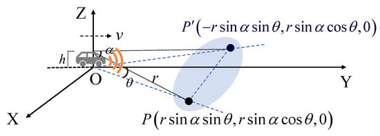
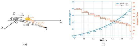
To analyze the nonlinear motion errors in long-aperture forward-looking imaging, a forward-looking radar imaging geometry model is established as shown in Figure 1. The radar platform is mounted on a moving platform at an altitude of h, flying at a constant velocity v along the Y-axis direction in a straight and level flight. The line connecting the target and the radar is defined as the radar line of sight (LOS). The beam pointing elevation angle $\alpha$ is defined as the angle between the radar LOS and the Z-axis, and the beam pointing azimuth angle $\theta$ is defined as the angle between the projection of the radar LOS onto the ground plane and the X-axis.

Figure 1. Geometric configuration of imaging scene.

Let the position of a target point in the scene be denoted by $P(rsin\alpha cos\theta ,rsin\alpha sin\theta ,0)$, with its corresponding symmetrical point relative to the Y-axis defined as $P^{\prime }$. As the radar platform traverses the flight path, its position becomes a function of slow time $t_m$. Specifically, the coordinates of the transmitting antenna and the i-th receiving antenna at $t_m$ are represented by $P_T(0,v{t}_m,h)$ and $P_{R_i}(x_i,v{t}_m,h)$, respectively. Consequently, the transmitting slant range $R_T$ to target P and the receiving slant range $R_R$ for the i-th channel can be formulated as follows:

$$R_T(t_m;r,\theta )={[{(rsin\alpha sin\theta )}^2+{(v{t}_m-rsin\alpha cos\theta )}^2+h^2]}^{1/2}$$

(1)

$$R_R(t_m,r,\theta ,x_i)={[{(x_i-rsin\alpha sin\theta )}^2+{(v{t}_m-rsin\alpha cos\theta )}^2+h^2]}^{1/2}$$

(2)

where $x_i$ represents the azimuth coordinate of the i-th receiving antenna element.

The dual-way slant range is defined as $R(t_m;r,\theta ,x_i)=R_T(t_m;r,\theta )+R_R(t_m;r,\theta ,x_i)$. Considering that electromagnetic waves propagate at the speed of light—significantly exceeding the platform’s velocity—the “stop-and-go” model is typically employed for echo data collection. At each azimuth sampling instant, the radar transmits a signal from its current position, and the platform remains stationary until the reception of the echo is completed. After the reception is finished, the platform moves to the next sampling position, and this process is repeated to complete the full-aperture acquisition. The premise for this assumption is that the platform displacement within a single pulse period is much smaller than the range resolution cell, which is sufficiently reasonable for conventional-velocity scenarios in the short-range imaging case of this paper. This condition can be satisfied pulse-by-pulse during long-aperture synthesis, and the applicability will not degrade with the increase in integration time.

2.2. Echo Signal Model

The signal transmitted by the radar central antenna is a linear frequency modulation (LFM) pulse signal, which can be expressed as follows:

$$s\left(\tau \right)=\mathrm{rect}\left[{\displaystyle \frac{\tau }{T}}\right]exp\left(j2\pi f_c\tau +j\pi K_r{\tau }^2\right)$$

(3)

where $\tau$ denotes the fast time, $\mathrm{rect}(·)$ is the rectangular window function, T represents the time-domain width of the rectangular window function, $f_c$ is the operating carrier frequency of the transmitted signal, and $K_r$ denotes the frequency modulation slope.

Assume that the back-scattering coefficient of the point target is $\sigma$ and the azimuth window function is $\omega (·)$; then, the point-target echo received by the i-th receiving array element at the corresponding time can be expressed as follows:

$$\begin{array}{cc}\hfill & s_i(\tau ,t_m;r,\theta ,x_i)=\sigma ·\omega \left(t_m\right)·\mathrm{rect}\left({\displaystyle \frac{\tau -R(t_m;r,\theta ,x_i)/c}{T}}\right)\hfill \\ \hfill & ·exp\left[j2\pi f_c\left(\tau -{\displaystyle \frac{R(t_m;r,\theta ,x_i)}{c}}\right)\right]\hfill \\ \hfill & ·exp\left[j\pi K_r{\left(\tau -{\displaystyle \frac{R(t_m;r,\theta ,x_i)}{c}}\right)}^2\right]\hfill \end{array}$$

(4)

After down-conversion and pulse compression of the echo simulation signal, the baseband received signal of each channel is

$$\begin{array}{c}\hfill s_i\left(\tau ,t_m;r,\theta ,x_i\right)\approx \sigma ·w\left(t_m\right)·\mathrm{sinc}\left[B\left(\tau -{\displaystyle \frac{R(t_m;r,\theta ,x_i)}{c}}\right)\right]·exp\left[{\displaystyle \frac{-j2\pi R(t_m;r,\theta ,x_i)}{\lambda }}\right]\end{array}$$

(5)

where $\sigma$ denotes the back-scattering coefficient of the point target, $\omega \left(t_m\right)$ is the azimuth-direction sampling window function, B represents the effective bandwidth of the transmitted signal, c is the propagation velocity of electromagnetic waves in free space, and $\lambda$ stands for the operating carrier wavelength of the radar system; $\tau$ is the range-direction fast time, and $t_m$ denotes the azimuth-direction slow time.

After imaging processing of the echo $s(\tau ,t_m;r,\theta )$, the resulting image vector $\mathbf{S}$ is obtained. At this stage, the forward-looking imaging result suffers from left–right Doppler ambiguity. This issue can be resolved by employing beamforming techniques that leverage matrix $\mathbf{P}$, which is constructed from multi-channel steering vectors [29]. At least two receiving channels are required to realize left--right Doppler ambiguity resolution. The steering vector can be constructed from the echo phase differences among different channels to distinguish symmetric targets. The multi-channel array adopted in this paper can further improve the stability of ambiguity resolution as well as the sidelobe suppression performance.

However, the above model does not account for the nonlinear variation characteristics of the target slant range history under long-term coherent integration conditions. Under short-aperture conditions, the relative motion of the target can usually be approximated by a linear model, and the echo phase maintains good coherence throughout the aperture. However, as the synthetic aperture time increases, the higher-order terms in the target slant range history gradually become more significant, causing the echo phase to deviate from the ideal linear model. This leads to a nonlinear variation in the Doppler history, which further induces spectrum broadening and image defocusing. Therefore, it is necessary to conduct a quantitative analysis of the high-order nonlinear errors in the slant range history under long-aperture conditions.

According to Equation (5), by neglecting $x_i$, the Taylor expansion of the phase term $\varphi \left(t_m\right)$ at $t_m=0$ is derived as follows:

$$\begin{array}{cc}\hfill & \varphi \left(t_m\right)=-{\displaystyle \frac{2\pi }{\lambda }}R(t_m;r,\theta )\hfill \\ \hfill & \approx -{\displaystyle \frac{4\pi }{\lambda }}\left\{r-vsin\alpha cos\theta ·t_m+{\displaystyle \frac{v^2\left[{(rsin\alpha sin\theta )}^2+h^2\right]}{2r^3}}·t_m^2\right\}\hfill \end{array}$$

(6)

Based on the geometric relationship, the linear component of $t_m$ is compensated. The compensated slant range $R^{\prime }(t_m;r,\theta )$ as a function of time $t_m$ (or pulse index n) is given by the following:

$$\begin{array}{c}\hfill R^{\prime }(n)\approx 2·\left\{r-v(sin\alpha cos\theta -1)nT+{\displaystyle \frac{v^2\left[{(rsin\alpha sin\theta )}^2+h^2\right]}{2r^3}}{\left(nT\right)}^2\right\}\end{array}$$

(7)

The variation of the phase term $\varphi \left(n\right)$ with respect to the pulse index n is expressed as

$$\varphi \left(n\right)=-{\displaystyle \frac{2\pi }{\lambda }}{R}^{\prime }(n)$$

(8)

According to the relationship between the instantaneous Doppler frequency and the phase derivative, the instantaneous Doppler frequency of the target is obtained as follows:

$$\begin{array}{c}\hfill f_d\left(n\right)={\displaystyle \frac{1}{2\pi T}}{\displaystyle \frac{d\varphi \left(n\right)}{dn}}\approx {\displaystyle \frac{2vsin\alpha cos\theta }{\lambda }}-{\displaystyle \frac{2v^{2}T\left[{(rsin\alpha sin\theta )}^2+h^2\right]}{\lambda r^3}}n\end{array}$$

(9)

As the synthetic aperture time increases, the higher-order nonlinear terms in the target slant range history accumulate continuously, resulting in significant variations of the instantaneous Doppler centroid and Doppler frequency modulation rate with spatial position. The target energy spreads in the Doppler domain, leading to degradation of azimuth resolution and image defocusing. Under such circumstances, conventional motion compensation methods based on the global linear assumption are no longer applicable to long-aperture near-field forward-looking imaging scenarios.

3. Adaptive Segmentation-Based Coherent Reconstruction Algorithm

3.1. Sub-Aperture Signal Modeling and Mapping in Polar Coordinates

To suppress the high-order phase distortion caused by the long aperture, this paper divides the full-aperture nonlinear observation process into K non-overlapping sub-apertures, such that the observation process within each sub-aperture can be approximated as a locally quasi-stationary process. Let the full-aperture duration be $T_{all}$ and the duration of the k-th sub-aperture be $T_{sub,k}$, satisfying $T_{all}={\sum }_{k=1}^K{T}_{sub,k}$. Since this paper focuses on azimuth motion compensation, the influence of receiving array element spacing can be temporarily neglected. By setting $x_i=0$, the instantaneous dual-way slant range of the radar platform relative to the target within the k-th sub-aperture can be expressed as follows:

$$R_k(t_m;r_k,{\theta }_k)=2·{\left[{(r_{k}sin{\alpha }_{k}sin{\theta }_k)}^2+h^2+{(v{t}_m-r_{k}sin{\alpha }_{k}cos{\theta }_k)}^2\right]}^{1/2}$$

(10)

where $(r_k,{\theta }_k)$ represents the relative position of the target in the k-th segment.

To establish the signal mapping relationship between the k-th sub-aperture and the first sub-aperture, the temporal correlation between the two slant range histories needs to be clarified. Since the starting time of the k-th sub-aperture corresponds to the position on the observation time axis of the first sub-aperture shifted by the cumulative duration of the preceding $k-1$ sub-apertures, the slant range functions of the two sub-apertures satisfy the following:

$$\begin{array}{cc}\hfill & r_k={\displaystyle \frac{R_k(0;r_1,{\theta }_1)}{2}}=[{\left(r_{1}sin{\alpha }_{1}sin{\theta }_1\right)}^2+\hfill \\ \hfill & {\left(v·{\displaystyle \sum _{sub=1}^{k-1}}{T}_{sub}-r_{1}sin{\alpha }_{1}cos{\theta }_1\right)}^2+h^2{]}^{1/2}\hfill \end{array}$$

(11)

Furthermore, the relationship between $R_1(t_m;r_1,{\theta }_1)$ and $R_k(t_m;r_k,{\theta }_k)$ is established as follows:

$$R_k(t_m;r_k,{\theta }_k)=R_1\left(t_m+{\displaystyle \sum _{sub=1}^{k-1}}{T}_{sub};r_1,{\theta }_1\right)$$

(12)

By performing Taylor expansion on $R_1(t_m;r_1,{\theta }_1)$ and $R_1\left(t_m+{\sum }_{sub=1}^{k-1}{T}_{sub};r_1,{\theta }_1\right)$ at $t_m=0$, we can obtain

$$\left\{\begin{array}{c}{R}_1(t_m;r_1,{\theta }_1)\approx 2·r_1+2·\left(-sin{\alpha }_{1}cos{\theta }_1\right)v·t_m\hfill \\ R_1\left(t_m+{\displaystyle \sum _{sub=1}^{k-1}}{T}_{sub};r_1,{\theta }_1\right)\approx 2·r_k\hfill \\ +2·{\displaystyle \frac{\left(v·{\sum }_{sub=1}^{k-1}{T}_{sub}-r_{1}sin{\alpha }_{1}cos{\theta }_1\right)v}{r_k}}·t_m\hfill \\ +{\displaystyle \frac{v^2\left[{\left(r_{1}sin{\alpha }_{1}sin{\theta }_1\right)}^2+h^2\right]}{r_k^3}}·t_m^2\hfill \end{array}\right.$$

(13)

Ignoring the higher-order terms and retaining only the first-order terms, we obtain

$$R_k(t_m;r_k,{\theta }_k)\approx R_1(t_m;r_1,{\theta }_1)+2·\mathsf{\Delta }{r}_k+{\displaystyle \frac{2v^2·{\displaystyle \sum _{sub=1}^{k-1}}{T}_{sub}}{r_k}}·t_m$$

(14)

which reflects the distortions in the slant range and azimuth angle, respectively. Here, $\mathsf{\Delta }{r}_k=r_k-r_1$.

Substituting Equation (14) into the echo Equation (5), the approximate relationship between the echo of the k-th sub-aperture and that of the first sub-aperture for the i-th receiving array element can be obtained as follows:

$$\begin{array}{cc}\hfill & {\mathbf{S}}_{ik}\left(t_r,t_m,r_k,{\theta }_k;x_i\right)\approx {\mathbf{S}}_{i1}\left(t_r,t_m,r_1,{\theta }_1;x_i\right)\hfill \\ \hfill & ·exp\left(\mathrm{j}{\displaystyle \frac{4\pi }{\lambda }}\left(\mathsf{\Delta }{r}_k+{\displaystyle \frac{v^2·{\sum }_{sub=1}^{k-1}{T}_{sub}}{r_k}}·t_m\right)\right)\hfill \end{array}$$

(15)

Based on the echo mapping relationship in Equation (15), the geometric mapping relationship between the imaging coordinate systems of the two sub-apertures can be further derived as follows:

$$\left\{\begin{array}{c}{r}_k=r_1+\mathsf{\Delta }{r}_k\hfill \\ {\theta }_k=arccos\left({\displaystyle \frac{vsin\alpha cos{\theta }_1+\frac{v^2{\sum }_{sub=1}^{k-1}{T}_{sub}}{r_k}}{r_k}}\right)\hfill \end{array}\right.$$

(16)

Let $X_k$ and $X_1$ denote the imaging results of the k-th and first sub-apertures, respectively. Combined with the coordinate mapping in Equation (16), the correspondence between the two imaging results at the pixel level is given by the following:

$$X_k(r_k,{\theta }_k)=X_1(r_1,{\theta }_1)·exp\left(j{\displaystyle \frac{2\pi }{\lambda }}(r_k-r_1)\right)$$

(17)

By unifying the reference coordinate system to the first sub-aperture perspective and defining the target position $(r_1,{\theta }_1)$ in the first sub-aperture view as the reference target position $(r,\theta )$, Equation (16) can be rewritten as follows:

$$X_k\left(r+\mathsf{\Delta }{r}_k,arccos\left({\displaystyle \frac{vsin\alpha cos\theta +\frac{v^2{\sum }_{sub=1}^{k-1}{T}_{sub}}{r_k}}{r_k}}\right)\right)=X_1(r,\theta )·exp\left(j{\displaystyle \frac{2\pi }{\lambda }}(r_k-r)\right)$$

(18)

Equation (18) indicates that the mapping relationship between the two imaging results depends not only on the sub-aperture index k but also on the spatial coordinates $(r,\theta )$ of the target. Therefore, under full-scene conditions, a direct pixel-by-pixel correspondence between the two-dimensional matrices $X_k$ and $X_1$ cannot be established. To address this, we rearrange $X_k$ and $X_1$ into column vectors $\mathrm{vec}\left(X_k\right)$ and $\mathrm{vec}\left(X_1\right)$. The mapping between the two sub-apertures can then be expressed as follows:

$$\mathrm{vec}\left(X_1\right)=\mathbf{D}·\mathbf{W}·\mathrm{vec}\left(X_k\right)+n_k$$

(19)

where $\mathbf{W}$ is the resampling matrix, and $\mathbf{D}$ is the diagonal phase compensation matrix. The corresponding calculation formulas are provided in Appendix A.

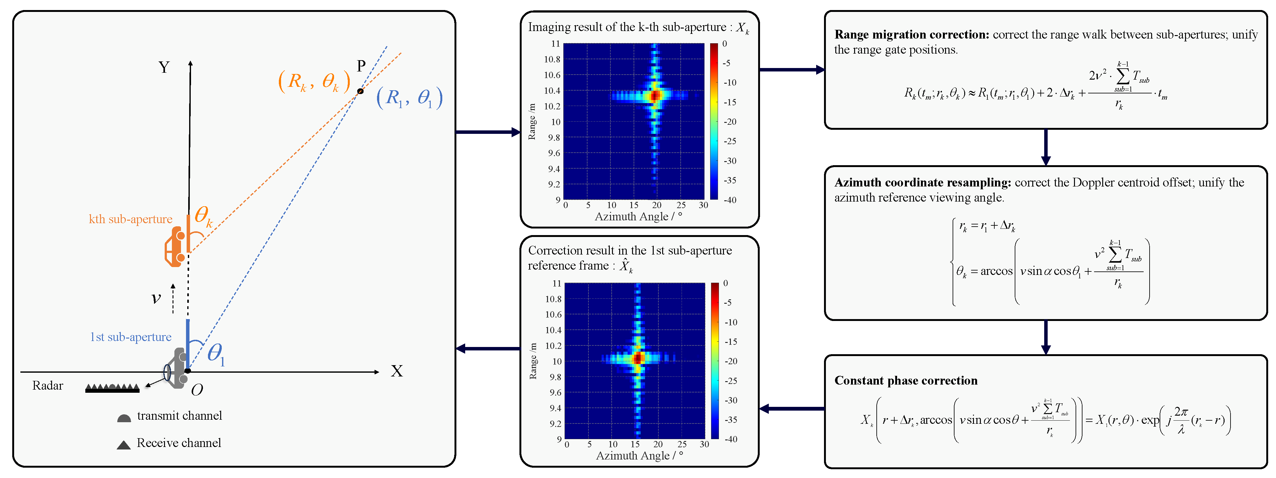
To intuitively demonstrate the coordinate mapping and signal correction process between adjacent sub-apertures, Figure 2 provides a schematic flowchart of cross-sub-aperture coordinate transformation. The overall transformation consists of three core procedures in sequence: range-domain slant-range correction, azimuth-domain angular resampling, and cross-segment phase compensation. Through these three operations, the imaging result of the k-th sub-aperture can be uniformly mapped onto the reference coordinate system of the first sub-aperture.

Figure 2. Schematic of cross-sub-aperture coordinate mapping transformation.

3.2. Adaptive Partitioning Criterion Constrained by Phase Errors

In sub-aperture imaging processing, the selection of coherent integration time directly determines the performance boundary between azimuth resolution and focusing fidelity. Its impact on imaging quality is primarily manifested in two dimensions: the azimuth Doppler characteristics and the range migration in the range direction. From the perspective of spatial scales, the range-domain constraint is typically governed by the range resolution cell ${\rho }_r$, while the azimuth phase exhibits wavelength-level $\lambda$ sensitivity to the slant range history variations caused by target motion. Since the nonlinear drift of the phase history occurs far earlier than the cross-cell migration of the geometric envelope, the coherence maintenance in the azimuth direction imposes a much stricter limitation on the integration time than the range migration constraint. Therefore, this section focuses on the analysis of the Doppler phase constraint in the azimuth direction.

The essence of azimuth resolution lies in the Doppler frequency difference arising from the relative motion between the radar and the target. An excessively short integration time results in insufficient Doppler observation duration, which broadens the azimuth resolution cell, renders adjacent scattering points indistinguishable, and directly causes azimuth image blurring. Conversely, an excessively long integration time introduces nonlinear Doppler variations driven by the non-uniform slant range history between the radar and the target, dispersing target energy in the Doppler domain and further inducing image defocusing. This section establishes the physical relationship between the time-varying Doppler chirp rate and the sub-aperture duration, and it derives an explicit segmentation constraint formula.

Section 3.1 established the first-order mapping relationship between the k-th sub-aperture and the first sub-aperture, which primarily corresponds to the range walk and Doppler shift. However, the more critical factor affecting focusing performance is the Doppler spectrum broadening caused by the second-order term. In the k-th sub-aperture, the echo phase is given by the following:

$${\mathrm{\Phi }}_k\left(t_m\right)={\displaystyle \frac{2\pi }{\lambda }}\left(R_k\left(t_m;r_k,{\theta }_k\right)+2v·{\displaystyle \sum _{sub=1}^{k-1}}{T}_{sub}\right)$$

(20)

Substituting into Equation (13), the formula for the spectrum broadening can be derived as follows:

$$\mathsf{\Delta }F=max\left({\displaystyle \frac{1}{2\pi }}{\displaystyle \frac{d{\mathrm{\Phi }}_k\left(t_m\right)}{d{t}_m}}\right)-min\left({\displaystyle \frac{1}{2\pi }}{\displaystyle \frac{d{\mathrm{\Phi }}_k\left(t_m\right)}{d{t}_m}}\right)t\in [0,T_k]$$

(21)

The zeroth-order term (fixed slant range offset) and the first-order term (linear Doppler component) in the Taylor expansion of the slant range history have been compensated via conventional motion compensation in Section 2.2, and they do not induce spectrum broadening. For terms of third order and above, since the expansion order of the slant range history corresponds one-to-one to the temporal power of the phase error, the additional phase error introduced by higher-order terms decays rapidly with increasing order. Its magnitude is far below the phase focusing tolerance, and the corresponding variation of the high-order Doppler chirp rate is insufficient to cause observable spectrum broadening. Therefore, the signal within each sub-aperture still satisfies the physical hypothesis of quasi-linear frequency modulation.

Accordingly, retaining only the second-order phase term in the modeling can fully ensure the accuracy of local compensation without introducing more complex high-order models. The adaptive segmentation criterion proposed in this section essentially constrains the Doppler nonlinearity caused by the second-order term, so that the signal in each sub-aperture physically approximates the ideal linear frequency modulation (LFM) model. The following equation is derived based on the Rayleigh criterion, which requires that the maximum residual high-order phase error within each sub-aperture shall not exceed $\pi /4$ radians. The second-order residual phase error is constrained as follows:

$$2\pi ·{\displaystyle \frac{v^2{T}_k^2\left[{(r_{1}sin{\alpha }_{1}sin{\theta }_1)}^2+h^2\right]}{8\lambda r_k^3}}\le {\displaystyle \frac{\pi }{4}}$$

(22)

The Rayleigh criterion provides a general physical basis for setting the upper bound of residual phase error within each sub-aperture. This error threshold is not a fixed value and can be flexibly selected according to the quality requirements of specific imaging scenarios, azimuth resolution specifications, and computational resource constraints. Adopting a stricter upper bound of phase error can further suppress nonlinear phase components inside sub-apertures and improve focusing accuracy. Nevertheless, it shortens the coherent integration duration of each segment, leading to the loss of azimuth resolution. Meanwhile, the increased number of sub-apertures raises the computational complexity of subsequent compensation. By contrast, a looser upper bound of phase error helps maintain a longer coherent integration window and superior azimuth resolution, as well as reduces the computational load of the algorithm. However, the residual nonlinear error within sub-apertures will increase correspondingly. In this paper, $\pi /4$ radians is adopted as the upper bound for residual phase error constraint. It is a classical engineering value in the SAR imaging field, which can achieve a reasonable balance among imaging focusing quality, azimuth resolution performance, and algorithm computational efficiency.

By rearranging Equation (22) and solving for $T_k$, we obtain the following:

$$T_k\le \sqrt{{\displaystyle \frac{2\pi \lambda r_k^3}{v^2\left[{\left(r_{1}sin{\alpha }_{1}sin{\theta }_1\right)}^2+h^2\right]}}}$$

(23)

According to the classical azimuth resolution theory for coherent imaging systems, azimuth resolution is inversely proportional to the coherent integration time [30] To maximize the coherent accumulation gain while satisfying the phase error constraint and achieve the optimal trade-off between focusing quality and resolution performance, the equality condition is adopted, which corresponds to the maximum allowable sub-aperture duration. Substituting the expression of $r_k$ from Equation (11), the explicit adaptive segmentation criterion is derived as follows:

$$\begin{array}{cc}\hfill T_k& ={\left[{\displaystyle \frac{\lambda }{v^2\left({(r_{1}sin{\alpha }_{1}sin{\theta }_1)}^2+h^2\right)}}\right]}^{1/2}\hfill \\ \hfill & ·{\left[{(r_{1}sin{\alpha }_{1}sin{\theta }_1)}^2+h^2+{\left(v{\displaystyle \sum _{sub=1}^{k-1}}{T}_{sub}-r_{1}sin{\alpha }_{1}cos{\theta }_1\right)}^2\right]}^{3/4}\hfill \end{array}$$

(24)

In practical radar systems, the radar observation geometry varies over different time intervals. The adaptive sub-aperture duration $T_k$ derived from the aforementioned constraints can be automatically lengthened or shortened according to the degree of nonlinearity. Under high-maneuver platform conditions or short-range detection modes, the nonlinear phase error increases rapidly, and the algorithm shortens $T_k$ accordingly; otherwise, the sub-aperture length is extended. This dynamic mechanism strictly limits the maximum residual phase error within each sub-aperture to below $\pi /4$, thus guaranteeing data consistency.

Furthermore, considering the hardware limitations of practical measurement instruments and platform maneuver disturbances, we assume instantaneous velocity measurement noise $\mathsf{\Delta }v$ induced by tiny platform vibrations. When this disturbance is substituted into the high-order Taylor expansion of the slant range, the resulting additional phase perturbation remains far smaller than the $\pi /4$ threshold defined by the adaptive criterion. This demonstrates that the proposed adaptive segmentation criterion not only satisfies the local quasi-linearity assumption theoretically, but it also possesses favorable fault tolerance against sampling uncertainties of real-world instruments and platform motion disturbances. Consequently, it enables fully controllable errors under complex industrial and field measurement scenarios.

3.3. Optimization of Compensation Operators Based on Operator Decoupling

The mapping operator $\mathbf{D}·\mathbf{W}$ in Equation (19) has extremely high dimensionality and exhibits range-azimuth cross-coupling. Direct inversion involves substantial computational cost and suffers from numerical instability. Noting that range-dimensional sampling and azimuth-dimensional phase correction can usually be decoupled into two independent processes, this paper equivalently transforms the vector-form mapping operator into a matrix-product form:

$${\mathbf{X}}_k\approx \mathbf{M}·{\mathbf{X}}_k·\mathbf{N}$$

(25)

where $\mathbf{M}\in {\mathbb{R}}^{P\times P}$ is the range compensation operator, responsible for correcting the range walk; $\mathbf{N}\in {\mathbb{R}}^{R\times R}$ is the azimuth compensation operator, used to eliminate the azimuth distortion caused by nonlinear motion.

The mapping operator $\mathbf{D}·\mathbf{W}$ in Equation (19) has an extremely high dimension and exhibits range-azimuth cross-coupling. Direct computation brings heavy computational burden and suffers from numerical instability. We formulate the compensation problem using a two-dimensional separable operator. Let the two-dimensional image matrix of the sub-aperture be ${\mathbf{X}}_k\in {\mathbb{C}}^{P\times R}$, where P denotes the number of range samples and R denotes the number of azimuth samples. Each column of the matrix corresponds to the range-dimension echo at one azimuth instant, and each row corresponds to the azimuth-dimension signal of one range gate.

The range-domain compensation operator $\mathbf{M}\in {\mathbb{C}}^{P\times P}$ corrects the range walk and range phase errors. Applying identical range-domain operations to all azimuth columns is equivalent to left-matrix multiplication: ${\mathbf{X}}_{DC}=\mathbf{M}·{\mathbf{X}}_k$. The azimuth-domain compensation operator $\mathbf{N}\in {\mathbb{C}}^{R\times R}$ compensates for azimuth nonlinear phase errors and coordinate offsets. Applying identical azimuth-domain operations to all range rows corresponds to right-matrix multiplication: ${\widehat{\mathbf{X}}}_k={\mathbf{X}}_{DC}·\mathbf{N}$. When the spatial variation within the sub-aperture is low, i.e., the range-compensation operator is independent of azimuth coordinates and the azimuth-compensation operator is independent of range coordinates, the two-dimensional compensation can be fully decoupled into a cascade form of left multiplication in the range domain and right multiplication in the azimuth domain: ${\widehat{\mathbf{X}}}_k=\mathbf{M}·{\mathbf{X}}_k·\mathbf{N}$.

The prerequisite for this separability assumption is that the spatial variation of operators within each sub-aperture can be neglected, which is exactly the physical condition guaranteed by the adaptive segmentation criterion. This approximation provides sufficient accuracy under conventional forward-looking imaging scenarios. It reduces the computational complexity from $O\left(P^2{R}^2\right)$ to $O\left(P^2\right)+O\left(R^2\right)$. For extreme scenarios such as large-squint wide-beam and ultra-short-range high-maneuver conditions, high-order range—azimuth coupling becomes prominent. The fully-separable approximation will yield accuracy degradation and the assumption no longer holds. Further optimization schemes such as weak-coupling correction terms should be introduced.

First, the problem is formulated as a least-squares form with a Frobenius norm constraint:

$$\underset{\mathbf{M}\in {\mathbb{R}}^{P\times P},\mathbf{N}\in {\mathbb{R}}^{R\times R}}{min}{\parallel \mathbf{N}·{\mathbf{X}}_k·\mathbf{M}-{\mathbf{X}}_k\parallel }_F^2$$

(26)

where ${\parallel ·\parallel }_F^2$ denotes the Frobenius norm of the matrix. The dimension of ${\mathbf{X}}_k$ is $P\times R$.

To decouple the multiplicative coupling between $\mathbf{M}$ and $\mathbf{N}$, an auxiliary variable $\mathbf{Z}=\mathbf{N}·{\mathbf{X}}_k$ is introduced, transforming the original problem into an optimization form with equality constraints:

$$\left\{\begin{array}{c}{\min }_{\mathbf{M},\mathbf{Z}}{\parallel \mathbf{Z}·\mathbf{M}-{\mathbf{X}}_k\parallel }_F^2\hfill \\ \mathrm{s}.\mathrm{t}.\mathbf{Z}-\mathbf{N}·{\mathbf{X}}_k=0\hfill \end{array}\right.$$

(27)

The augmented Lagrangian function is constructed as follows:

$$L_{\rho }\left(\mathbf{M},\mathbf{N},\mathbf{Z},\mathbf{\Lambda }\right)={∥\mathbf{Z}·\mathbf{N}-{\mathbf{X}}_1∥}_F^2+⟨\mathbf{\Lambda },\mathbf{Z}-\mathbf{M}·{\mathbf{X}}_k⟩+{\displaystyle \frac{\rho }{2}}{∥\mathbf{Z}-{\mathbf{X}}_k·\mathbf{N}∥}_F^2$$

(28)

Update of $\mathbf{M}$ (M-update): At iteration $(l+1)$, fix $\mathbf{N}={\mathbf{N}}^l$, $\mathbf{Z}={\mathbf{Z}}^l$, and $\mathbf{\Lambda }={\mathbf{\Lambda }}^l$. Observe that among the three terms in Equation (28), only the fidelity term $\parallel \mathbf{Z}\mathbf{M}-{\mathbf{X}}_1{\parallel }_F^2$ contains the variable $\mathbf{M}$; the inner-product term and the quadratic penalty term are both independent of $\mathbf{M}$ and can be treated as constants. The M-subproblem reduces to

$${\mathbf{M}}^{l+1}=\arg \underset{\mathbf{M}}{\min }{∥{\mathbf{Z}}^l\mathbf{M}-{\mathbf{X}}_1∥}_F^2.$$

(29)

Define the cost function $J\left(\mathbf{M}\right)=\parallel {\mathbf{Z}}^l\mathbf{M}-{\mathbf{X}}_1{\parallel }_F^2$. Expand the Frobenius norm:

$$J\left(\mathbf{M}\right)=\mathrm{tr}\left[{\left({\mathbf{Z}}^l\mathbf{M}-{\mathbf{X}}_1\right)}^{\mathrm{T}}\left({\mathbf{Z}}^l\mathbf{M}-{\mathbf{X}}_1\right)\right].$$

(30)

Using the matrix derivative identity ${\displaystyle \frac{\partial }{\partial \mathbf{M}}}{\parallel \mathbf{Z}\mathbf{M}-\mathbf{X}\parallel }_F^2=2{\mathbf{Z}}^{\mathrm{T}}(\mathbf{Z}\mathbf{M}-\mathbf{X})$, the gradient with respect to $\mathbf{M}$ is

$${\nabla }_{\mathbf{M}}J\left(\mathbf{M}\right)=2{\left({\mathbf{Z}}^l\right)}^{\mathrm{T}}\left({\mathbf{Z}}^l\mathbf{M}-{\mathbf{X}}_1\right).$$

(31)

Setting the gradient to zero (first-order optimality condition),

$${\left({\mathbf{Z}}^l\right)}^{\mathrm{T}}{\mathbf{Z}}^l\mathbf{M}={\left({\mathbf{Z}}^l\right)}^{\mathrm{T}}{\mathbf{X}}_1.$$

(32)

Assuming ${\left({\mathbf{Z}}^l\right)}^{\mathrm{T}}{\mathbf{Z}}^l$ is invertible, the closed-form least-squares solution is as follows:

$${\mathbf{M}}^{l+1}={\left[{\left({\mathbf{Z}}^l\right)}^{\mathrm{T}}{\mathbf{Z}}^l\right]}^{-1}{\left({\mathbf{Z}}^l\right)}^{\mathrm{T}}{\mathbf{X}}_1$$

(33)

The derivations for N-update and Z-update follow exactly the same logic described above. After fixing the remaining variables, we compute the matrix partial derivatives with respect to $\mathbf{N}$ and $\mathbf{Z}$, respectively, and set the derivatives to zero, which yields the corresponding closed-form update formulas. The dual variable $\mathbf{\Lambda }$ is updated following the standard gradient-ascent rule of ADMM. At the $(l+1)$-th iteration, the variables are updated as Table 1.

Table 1. ADMM iterative update procedure.

Update Step	Formula
M-update	${\mathbf{M}}^{l+1}={\left[{\left({\mathbf{Z}}^l\right)}^{\mathrm{T}}{\mathbf{Z}}^l\right]}^{-1}{\left({\mathbf{Z}}^l\right)}^{\mathrm{T}}{\mathbf{X}}_1$
N-update	${\mathbf{N}}^{l+1}=\left({\mathbf{Z}}^l+{\displaystyle \frac{1}{\rho }}{\mathbf{\Lambda }}^l\right){\mathbf{X}}_k^{\mathrm{T}}{\left({\mathbf{X}}_k{\mathbf{X}}_k^{\mathrm{T}}\right)}^{-1}$
Z-update	${\mathbf{Z}}^{l+1}=\left[{\mathbf{\Lambda }}^l+\rho {\mathbf{N}}^{l+1}{\mathbf{X}}_k+2{\mathbf{X}}_1{\left({\mathbf{M}}^{l+1}\right)}^{\mathrm{T}}\right]·{\left[2{\mathbf{M}}^{l+1}{\left({\mathbf{M}}^{l+1}\right)}^{\mathrm{T}}+\rho \mathbf{I}\right]}^{-1}$
Dual variable update	${\mathbf{\Lambda }}^{l+1}={\mathbf{\Lambda }}^l+\rho \left({\mathbf{Z}}^{l+1}-{\mathbf{N}}^{l+1}{\mathbf{X}}_k\right)$
Convergence criterion	The iteration terminates when ${∥{\mathbf{Z}}^{l+1}-{\mathbf{N}}^{l+1}{\mathbf{X}}_k∥}_{\mathrm{F}}<\epsilon$, where $\epsilon$ is the preset convergence tolerance.

The penalty parameter $\rho$ is set to the classical domain-specific value $\rho =1.00$ to balance convergence speed and numerical stability. The primal residual is adopted as the convergence criterion. Iterations terminate when the residual is smaller than the convergence threshold $\epsilon =1\times {10}^{-4}$. This threshold is a commonly-used engineering value for iterative SAR imaging processing, which achieves a favorable trade-off between imaging accuracy and computational efficiency. After the iteration converges, the optimal operators $\widehat{\mathbf{M}}$ and $\widehat{\mathbf{N}}$ are substituted into Equation (25) to obtain the compensated and calibrated full-aperture imaging result.

From the perspective of regularization, the penalty parameter $\rho$ is inherently equivalent to Tikhonov numerical regularization. Taking the closed-form solution of the N-update sub-problem as an example, the term ${\displaystyle \frac{1}{\rho }}\mathbf{I}$ inside the matrix inversion is the standard Tikhonov regularization term. It prevents the covariance matrix ${\mathbf{X}}_k{\mathbf{X}}_k^{\mathrm{H}}$ from becoming ill-conditioned or singular, improves the numerical stability of iterative solving, suppresses high-frequency fluctuations of the compensation operator, and avoids over-fitting of the solution. Combined with the physical constraint brought by pre-adaptive segmentation, the rationality of the solution and algorithm robustness are guaranteed from both numerical and physical perspectives.

4. Experimental Results and Performance Analysis

To verify the effectiveness of the proposed adaptive-segmentation compensation algorithm for large-aperture forward-looking imaging, its performance is evaluated in this section from two perspectives: resolution preservation capability and energy focusing performance. First, quantitative analysis is carried out via point-target simulations. The azimuth resolution performance is quantified by the Full Width at Half Maximum (FWHM). Meanwhile, the focusing quality is comprehensively assessed using the Peak Sidelobe Ratio (PSLR), Integrated Sidelobe Ratio (ISLR), and Energy Concentration Ratio (ECR). Second, the reconstruction capability for complex scenes is validated. Extended-target simulation experiments are performed, and image entropy is adopted as the evaluation metric to verify the engineering practicability of the algorithm.

4.1. Point-Target Simulation

In this section, the ultimate focusing performance of the proposed method under ideal conditions is quantitatively evaluated through point-target simulations. All simulations in this paper are implemented using MATLAB R2020a (MathWorks, Natick, MA, USA). The simulation parameters are listed in Table 2.The point-target is located at $(10\mathrm{m},15°)$ in the radar platform relative coordinate system, and the total number of accumulated pulses over the full aperture is 3000. Combined with the pulse repetition frequency of 5 kHz given in Table 2, the corresponding synthetic-aperture time is 0.6 s.

Table 2. Simulation system parameters.

Parameter Category	Parameter Name	Value
Time Resource and Array Configuration	Total Pulse Repetition Frequency (PRF)	5 kHz
	Number of Transmit Antennas	1
	Number of Receive Antennas	8
	Pulse Repetition Time (PRT)	0.2 ms
Transmit Signal Waveform	Carrier Frequency	77 GHz
	Chirp Rate	$1.17\times {10}^{14}$ Hz/s
	Effective Signal Pulse Width	$12.8\mathsf{\mu }\mathrm{s}$
	Signal Bandwidth	1.5 GHz
Motion Parameters	Platform Velocity	10 m/s
Sampling and Processing	Dechirped Sampling Rate	20 MHz
	Fast Time Sampling Points	512

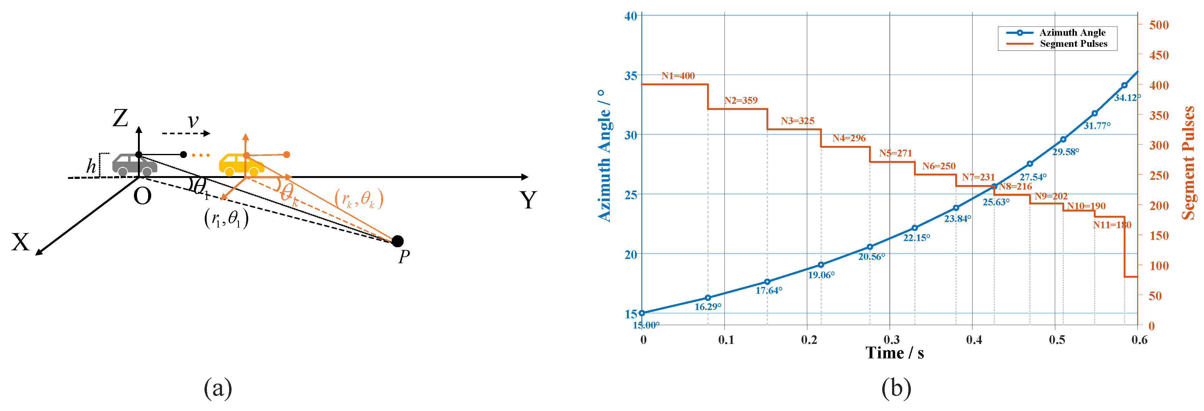
According to the adaptive segmentation criterion in Equation (24), the initial reference point is set at the slant-range of the geometric center of the imaging scene and half of the azimuth observation range. The adaptive segmentation scheme is illustrated in Figure 3. Figure 3a shows the geometric relationship of sub-aperture division, and Figure 3b presents the pulse-number sequence of each sub-aperture together with the corresponding instantaneous azimuth angles. After segment-by-segment partitioning according to the adaptive segmentation criterion, eleven valid sub-apertures are finally obtained, containing a total of 2920 pulses. Upon finishing the 11-th segment (180 pulses), the theoretically required number of pulses for the next segment calculated from the phase-nonlinearity constraint is 172. However, only 80 pulses remain in the full aperture, which cannot satisfy the minimum-length requirement for this segment. Considering that an insufficient pulse count will result in an inadequate effective synthetic-aperture length for the corresponding sub-aperture, which substantially degrades azimuth resolution, broadens the main lobe and raises sidelobe levels, and consequently impairs the overall imaging performance of cross-segment coherent reconstruction, the algorithm discards these trailing residual pulses as invalid aperture data and excludes them from subsequent imaging processing. It can be observed that the degree of phase nonlinearity gradually intensifies as the target azimuth angle increases. The number of pulses within each segment exhibits a decreasing trend, dropping progressively from 400 pulses in the first segment to 180 pulses in the 11-th segment. This validates the responsiveness of the proposed adaptive criterion to variations in the severity of phase nonlinearity.

Figure 3. Adaptive partitioning scheme. (a) Schematic of the aperture partitioning scenario. (b) Full-process monitoring diagram of the adaptive partitioning scheme.

From the perspective of physical mechanism, a larger target azimuth angle leads to higher second-order curvature of the slant-range history. The nonlinear component of the Doppler chirp rate accumulates more rapidly with coherent integration time. Constrained by the unified residual phase error tolerance, the effective coherent integration window satisfying the Rayleigh phase criterion becomes shorter, and consequently fewer pulses can be accommodated within a single sub-aperture. It can be observed that the degree of phase nonlinearity gradually intensifies as the target azimuth angle increases. The pulse number of each sub-aperture exhibits a decreasing trend, gradually dropping from 400 pulses in the first segment to 180 pulses in the last segment. This variation is in good agreement with the theoretical derivation, which verifies that the proposed adaptive segmentation criterion can accurately respond to the spatial variation of phase-nonlinearity severity.

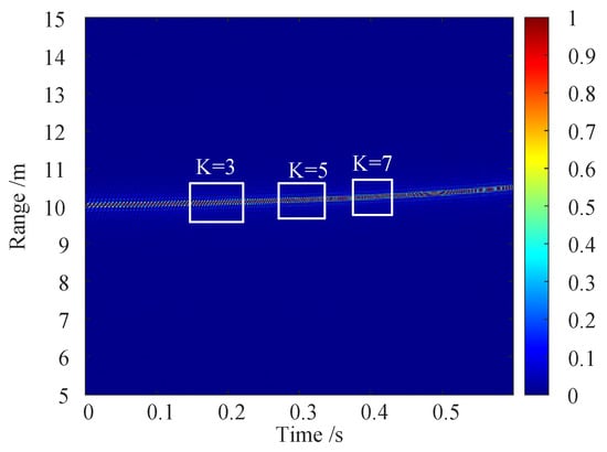
Figure 4 illustrates the variation of the target slant range over time under the long-aperture condition. The target position across different sub-apertures exhibits significant cross-range-cell migration along the slant range direction, and the migration amount increases with the extension of the aperture. To verify the correction effect of the proposed segmentation compensation method on this migration, Figure 5 compares the range-Doppler (R-D) maps of the 3rd, 5th, and 7th sub-apertures before and after compensation. Before compensation, the centroid position of the target in each sub-aperture shifts with the accumulation time, and the degree of azimuth broadening gradually increases. After compensation, the targets in each sub-aperture are precisely resampled to a unified reference position, the centroid offset is compensated, and the azimuth focusing patterns tend to be consistent.

Figure 4. Range–time image.

Figure 5. Intra-segment Range-Doppler (RD)maps before and after compensation. (a) RD map of the 3rd segment before compensation. (b) RD map of the 5th segment before compensation. (c) RD map of the 7th segment before compensation. (d) RD map of the 3rd segment after compensation. (e) RD map of the 5th segment after compensation. (f) RD map of the 7th segment after compensation.

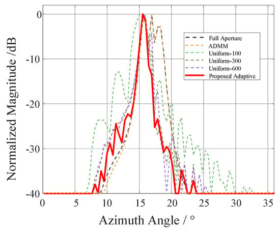
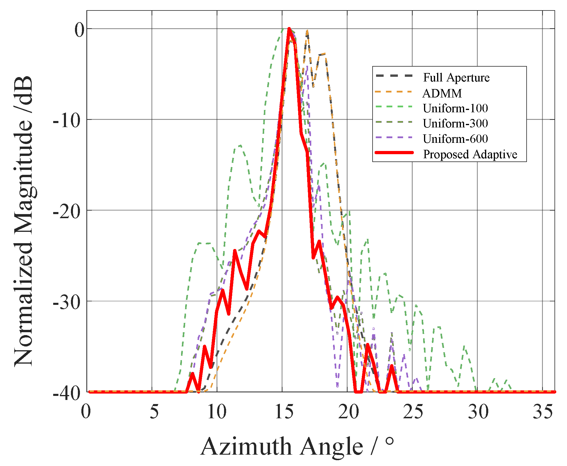
To verify the advantages of the adaptive segmentation strategy over fixed strategies, this paper compares five processing schemes: full-aperture direct imaging, global ADMM compensation, uniform segmentation (100/300/600 pulses per segment), and the proposed adaptive segmentation. Figure 6 presents the PSF of the azimuth profiles of the point target under each scheme, and the corresponding quantitative metrics are listed in Table 3.

Figure 6. Point-Spread Function (PSF) results of azimuth profiles of point targets under different imaging schemes.

Table 3. Imaging performance comparison of different processing methods.

Processing Method	PSLR (dB)	ISLR (dB)	FWHM	ECR	Elapsed Time/s
full-aperture	−6.61	5.58	3.50	0.15	2.08
Global Alternating Direction Method of Multipliers (ADMM) compensation (without segmentation)	−6.61	5.56	3.49	0.15	2.13
Uniform Segmentation: 100 Pulses/Segment	−3.55	7.13	4.50	0.12	23.825
Uniform Segmentation: 300 Pulses/Segment	−6.51	6.60	3.00	0.14	6.997
Uniform Segmentation: 600 Pulses/Segment	−6.61	5.57	3.50	0.15	3.345
First Segment of Adaptive Segmentation	−2.94	5.57	4.00	0.12	1.076
Proposed Adaptive Segmentation	−6.66	5.54	3.00	0.18	7.502

Notes: Peak Sidelobe Ratio (PSLR); Integrated Sidelobe Ratio (ISLR); Full Width at Half Maximum (FWHM); Energy Concentration Ratio (ECR). Bold values represent the optimal result for each evaluation metric.

Full-aperture direct imaging suffers from high-order nonlinear phase effects, with the main lobe broadening to 3.50, a PSLR of only −6.61 dB, and an energy concentration of only 0.15, indicating severe energy dispersion. Although the global ADMM compensation improves some sidelobes through iterative optimization, the full-aperture signal has already exceeded the applicable range of the linear operator, resulting in no significant improvement in main-lobe width or energy concentration. Among the fixed segmentation schemes, the 100 pulses/segment scheme ensures the local linear assumption, but the excessively short single-segment accumulation time broadens the FWHM to 4.50, leading to severe azimuth resolution degradation. The 300 pulses/segment scheme compresses the FWHM broadening to 3.00, but its ISLR reaches −6.60 dB and the energy concentration is only 0.14, indicating that inter-segment mismatches elevate the sidelobe energy. The 600 pulses/segment scheme approaches the full-aperture case, where nonlinear errors re-accumulate, and the performance is comparable to that of the full-aperture scheme. In contrast, the proposed adaptive segmentation achieves superior performance in all metrics compared with all the competing schemes, demonstrating that the adaptive criterion achieves the optimal balance between accumulation gain and phase fidelity.

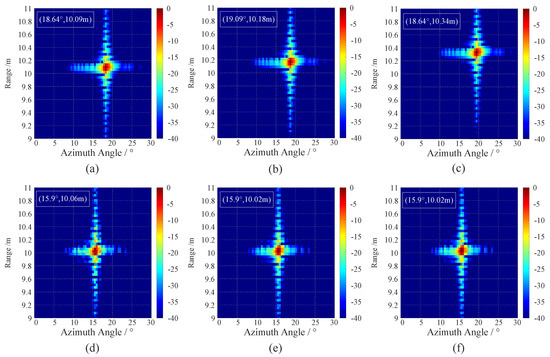
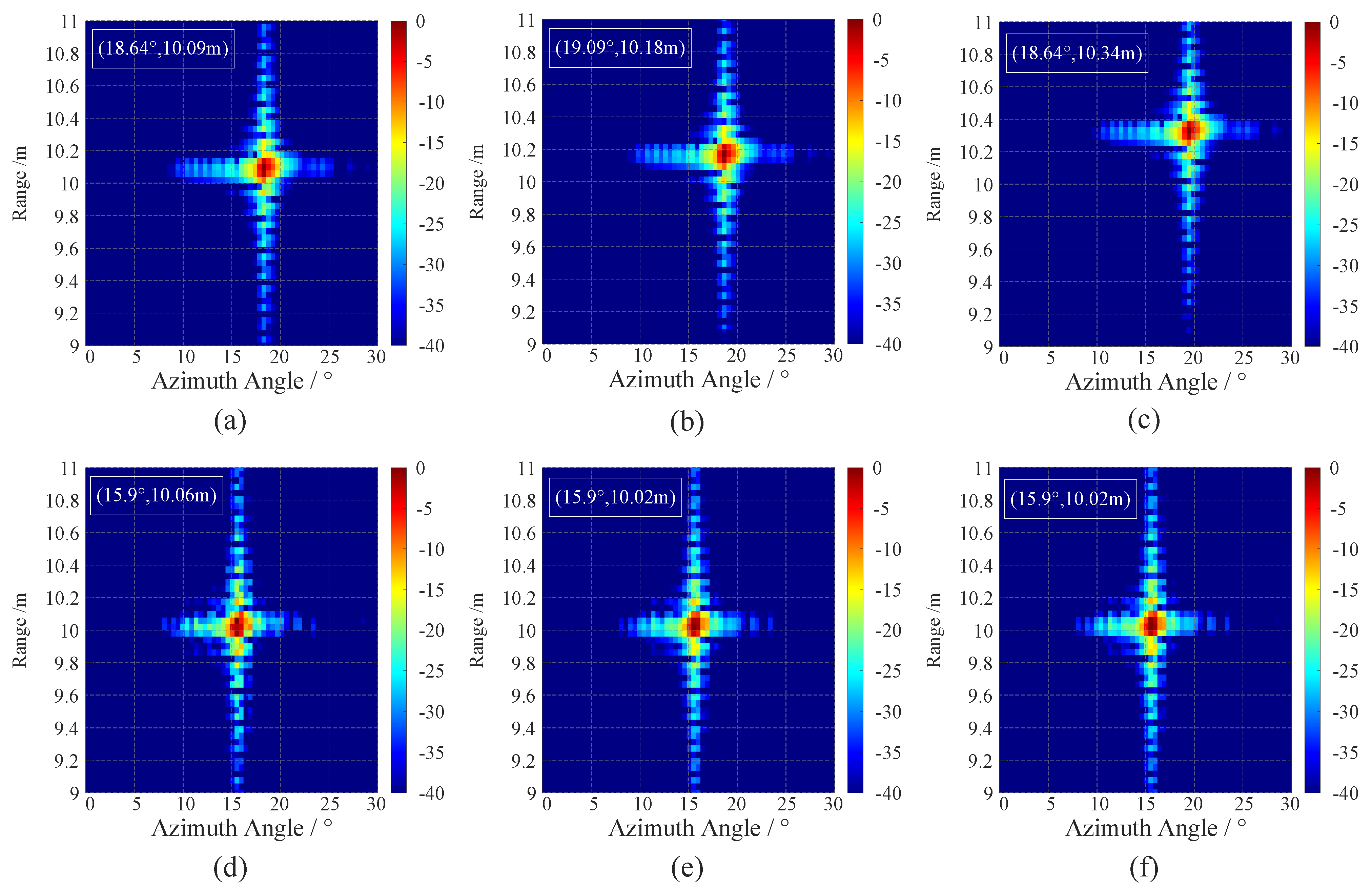
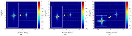
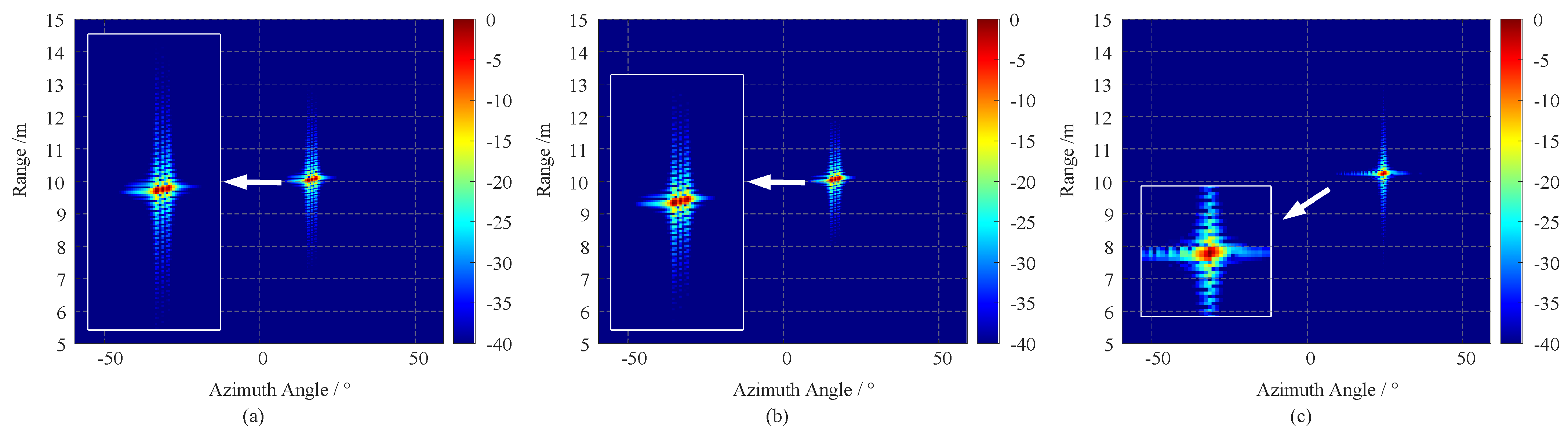
Figure 7 presents a two-dimensional imaging comparison of the three methods. In the full-aperture direct imaging result shown in Figure 7a, the target energy is severely diffused in the azimuth direction, making it impossible to distinguish valid peaks. In the global ADMM compensation result shown in Figure 7b, although the sidelobes are reduced, the main-lobe blurring is not eliminated. In contrast, the proposed method achieves clear focusing of the target in Figure 7c, with a narrow main lobe and low sidelobes, which is consistent with the quantitative conclusions presented in Table 3. The table supplements the single-frame processing time of each method under the identical hardware platform. It can be observed that full-aperture-type methods feature the lowest computational complexity yet deliver the poorest imaging performance. The time consumption of uniform-segmentation methods increases with the number of segments. The proposed method only incurs an extra ∼7.2% processing latency compared with the uniform-segmentation scheme of comparable segmentation granularity, while achieving cross-segment coherent reconstruction and remarkable improvement in focusing performance, which yields prominent overall cost-performance.

Figure 7. Simulation results of single point target. (a) Full-aperture imaging. (b) Direct compensation using alternating direction method of multiplier (ADMM). (c) Segmented compensation with the proposed method.

4.2. Extended-Target Simulation

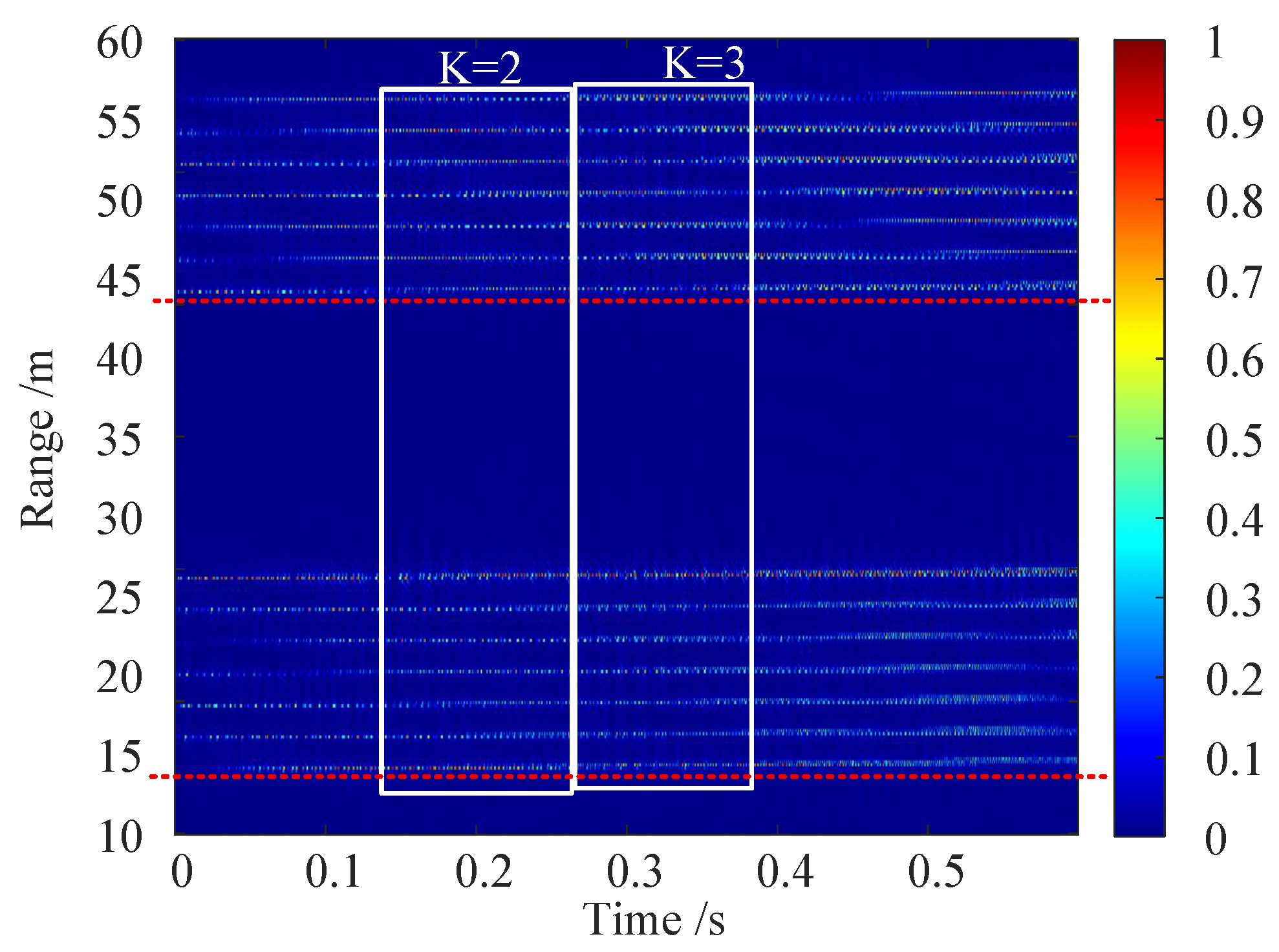
To further verify the overall focusing capability of the algorithm for spatially distributed targets, In the extended-target simulation of this section, 80 point scatterers with fixed radar cross-section (RCS) are used to construct an “NUDT”-shaped target for verifying the imaging reconstruction capability of the proposed algorithm for extended scenes. No thermal noise is added to the simulation background to exclude irrelevant impacts induced by amplitude-domain random disturbances and purely reveal the inherent phase-compensation performance and contour reconstruction capability of the algorithm. The scatterers are distributed over the slant range from 10 m to 30 m, covering the main illumination region of the radar beam. The simulation parameters are consistent with those in Section 4.1. The full aperture contains 3000 echoes, which are divided into five sub-apertures according to the adaptive criterion. The pulse counts for the sub-apertures are 692, 651, 614, 580, and 463, respectively, as shown in Figure 8.

Figure 8. Range–time image of extended target.

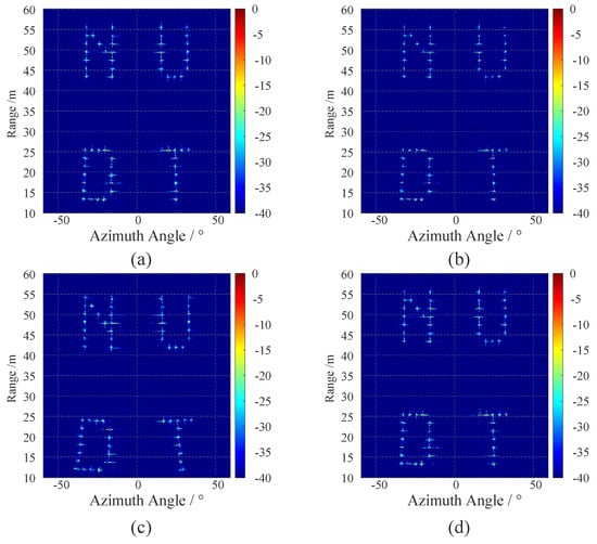
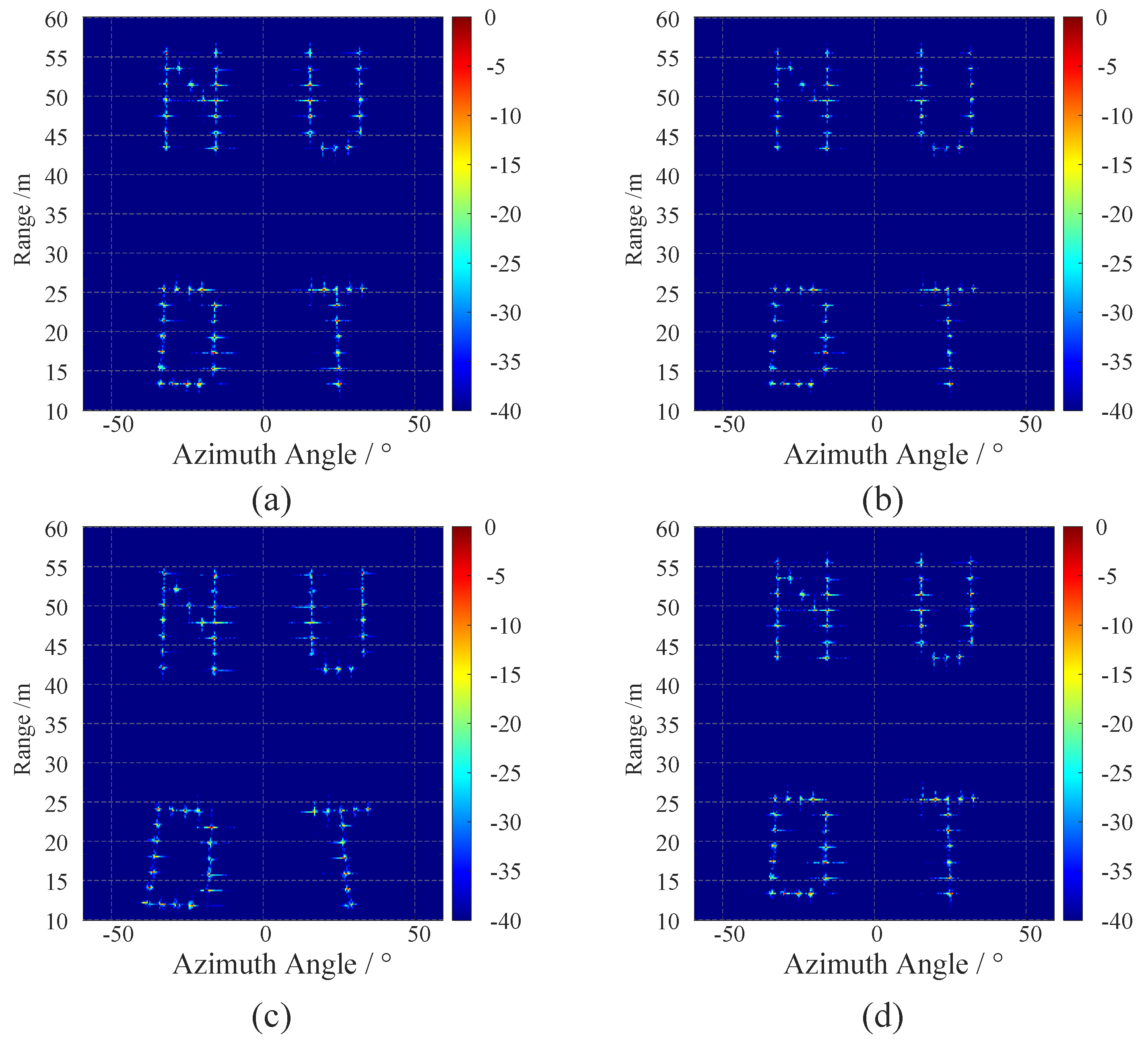
Figure 9 presents a comparison of the R-D maps of the 2nd and 3rd sub-apertures before and after compensation. Before compensation, due to the differences in the Doppler frequency modulation rates of targets at different spatial positions under the long-aperture condition, the letter array exhibits nonlinear spatial distortion. The nearby letter ‘T’ suffers more severe distortion than the distant letter ‘N’ which is consistent with the theoretical analysis that the spatially variant phase error increases with the slant range. After compensation, the targets in both sub-apertures are precisely resampled to a unified coordinate system, the geometric topological relationships of the letters are rigorously restored, and the inter-segment stitching is well achieved with no obvious misalignment.

Figure 9. Range-Doppler (RD) maps before and after intra-segment compensation. (a) RD map of the second segment before compensation. (b) RD map of the second segment after compensation. (c) RD map of the third segment before compensation. (d) RD map of the third segment after compensation.

For extended targets, point-based evaluation metrics are no longer applicable; instead, this paper adopts image entropy to measure the focusing performance. A lower image entropy value for the corresponding extended-target image indicates that the target energy is more concentrated and the defocusing suppression effect is better. To ensure a fair comparison, the image entropy E in this paper is computed after normalizing the matrix. For a discretized complex image matrix, the image entropy E is defined as follows:

$$E=-{\displaystyle \sum _{i=1}^{N_r}}{\displaystyle \sum _{j=1}^{N_m}}P(i,j)ln\left[P(i,j)\right]$$

(34)

where $N_r$ and $N_m$ denote the number of sampling points in the range dimension and azimuth dimension, respectively. $P(i,j)$ represents the normalized energy probability density at the $(i,j)$-th pixel of the image, and its calculation formula is as follows:

$$P(i,j)={\displaystyle \frac{{\left|\mathbf{X}(i,j)\right|}^2}{{\sum }_{i=1}^{N_r}{\sum }_{j=1}^{N_m}{\left|\mathbf{X}(i,j)\right|}^2}}$$

(35)

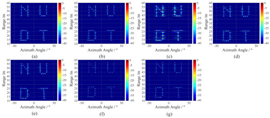
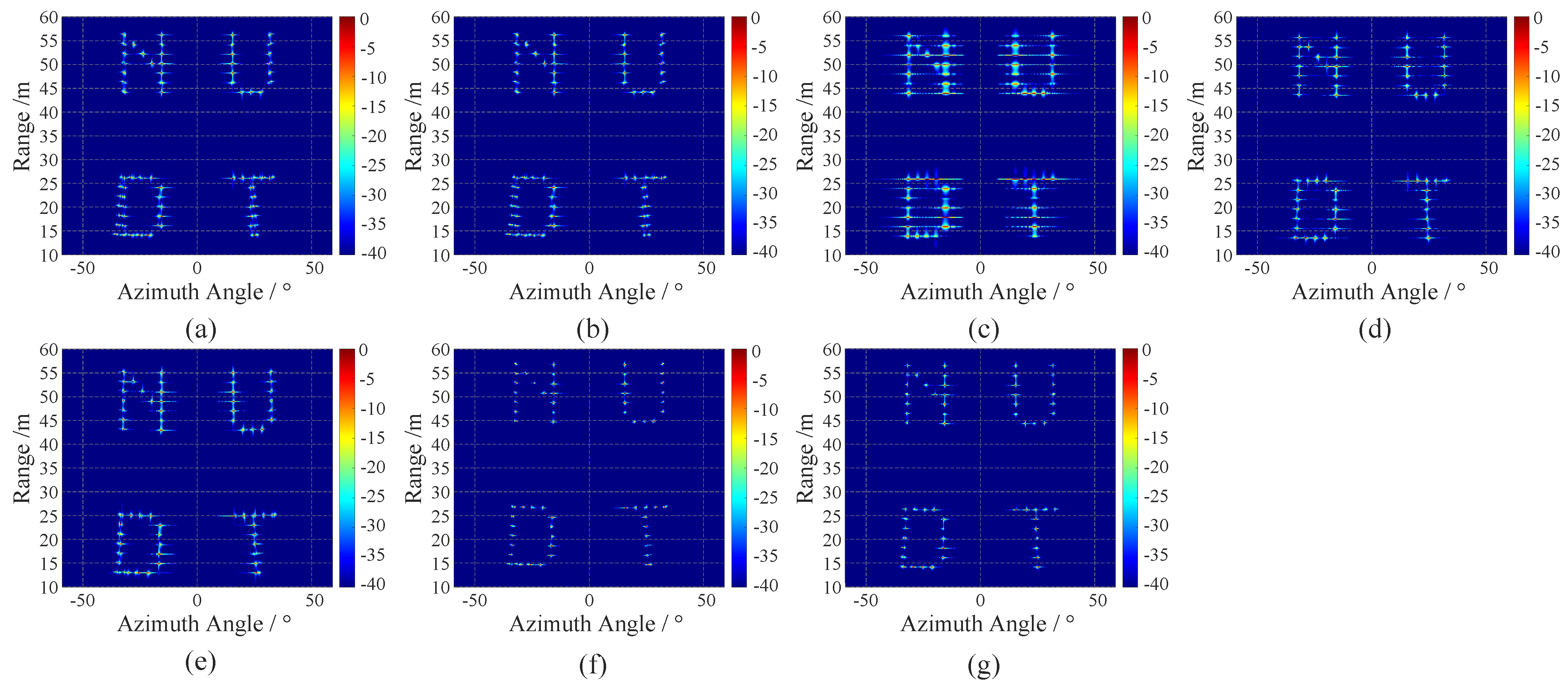
The processing results of the four schemes are shown in Figure 10, and the corresponding image entropy values are listed in Table 4.

Figure 10. Comparison of extended-target imaging results obtained by different imaging algorithms. (a) Full-aperture direct imaging; (b) global Alternating Direction Method of Multipliers (ADMM) compensation; (c) 100-pulse uniform segmentation;(d) 300-pulse uniform segmentation; (e) 600-pulse uniform segmentation; (f) Proposed adaptive segmentation method; (g) Reference-point optimized adaptive segmentation method.

Table 4. Image entropy of imaging results obtained by different processing methods.

Processing Method	Image Entropy
Full-aperture without segmentation	7.3493
Global Alternating Direction Method of Multipliers (ADMM) compensation (without segmentation)	6.7597
Uniform segmentation: 100 pulses/segment	7.5162
Uniform segmentation: 300 pulses/segment	6.3175
Uniform segmentation: 600 pulses/segment	6.5249
Adaptive segmentation (single-side center)	6.1493
Adaptive segmentation (near-field center)	6.0877

Table 4 lists the image entropy values of different imaging algorithms. Compared with the full-aperture non-segmented scheme (7.3493), the global ADMM compensation reduces the image entropy by 8.0%, verifying that iterative optimization can partially suppress phase nonlinear defocusing. Among the fixed-length segmentation baselines, the 100-pulse segmentation yields higher entropy (7.5162) than the full-aperture case, since excessive segmentation degrades the coherent accumulation gain. By contrast, the 300-pulse and 600-pulse uniform segmentations achieve lower entropy values of 6.3175 and 6.5249, respectively, where the 300-pulse scheme presents the best focusing performance among all fixed-length baselines. Benefiting from the dynamically adjusted segment length, the proposed adaptive segmentation further minimizes the image entropy. The optimal result reaches 6.0877, which is 10.0% lower than global ADMM compensation and 3.6% lower than the best fixed-length baseline (300-pulse uniform segmentation). In addition, the entropy difference between the single-side-center and near-field-center adaptive schemes is less than 1.5%, demonstrating that the proposed algorithm is insensitive to the selection of the reference point and exhibits excellent spatial robustness and generalization capability.

4.3. Measured-Data Results

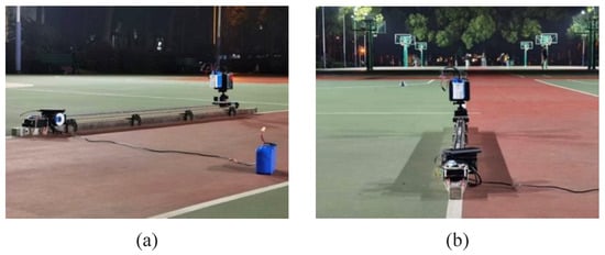
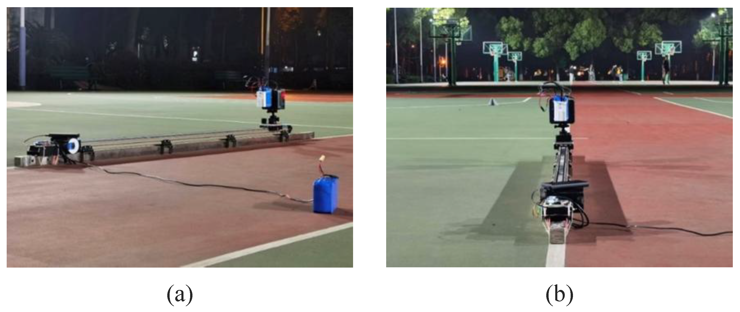
To verify the effectiveness of the algorithm under practical system conditions, a rail-based forward-looking radar experimental platform is constructed in this section, as shown in Figure 11. The radar array is mounted on a rail, and the motor drives the radar platform to move forward at a constant speed to detect targets in the forward-looking imaging region. The relevant parameters are listed in Table 5.

Figure 11. Experimental scenario and setup. (a) Experimental equipment. (b) Imaging scenario.

Table 5. Experimental parameter settings.

Parameter Category	Parameter Name	Value
Rail Information	Rail Length	1.9 m
	Speed Range	0–0.0556 m/s
Radar Array Information	Number of Transmit Antennas	2
	Number of Receive Antennas	4
Radar System Parameters	Pulse Repetition Frequency (PRF)	20 Hz
	System Center Frequency $f_0$	77 GHz
	System Chirp Rate $K_r$	30 MHz/$\mathsf{\mu }$s
	Sampling Frequency $f_s$	20 MHz

Taking the forward direction of the radar platform as the y-axis and the radar distribution direction as the x-axis, two corner reflectors are placed in the imaging scene as calibration targets, with the polar coordinates of the target positions at $(10\mathrm{m},15°)$ and $(15\mathrm{m},10°)$. The platform moves at approximately 0.0556 m/s. In field experiments, the guide-rail system is started first, and radar sampling is activated only after the platform motion becomes fully stable. Thus, the raw echo data can be regarded as being acquired entirely under uniform-motion conditions. Under such an extremely low-speed uniform-motion condition, the amplitudes of range-direction disturbances caused by guide-rail mechanical vibration and slow-time phase errors induced by motor speed ripple are very low. They are much smaller than the geometry-variation-dominated phase-nonlinear error in large-aperture forward-looking imaging, and their effects on the final focusing performance and the compensation accuracy of the ADMM algorithm are negligible. Therefore, no dedicated preprocessing step is configured for these weak mechanical disturbances in the algorithm processing pipeline.

It should be supplemented that the aforementioned point-target and extended-target simulations are performed at a platform velocity of $10 \mathrm{m}/\mathrm{s}$, covering the short-range high-maneuver imaging scenario and sufficiently validating the core performance of the proposed algorithm. The measurement experiment in this section emphasizes the verification of engineering applicability and robustness of the algorithm under a real-world radar system, which forms complementary validation with the simulation experiments. Restricted by the motion parameters of the laboratory rail platform, this experiment conducts proof-of-principle validation under the constant velocity of $0.0556 \mathrm{m}/\mathrm{s}$ so as to test the stable operation capability of the algorithm in the presence of practical sampling noise and tiny platform perturbations. A rail-borne forward-looking radar imaging platform is constructed, as shown in Figure 10. The radar array is mounted on the rail slider and driven by a motor to move forward at a constant speed to detect targets within the forward-looking region.

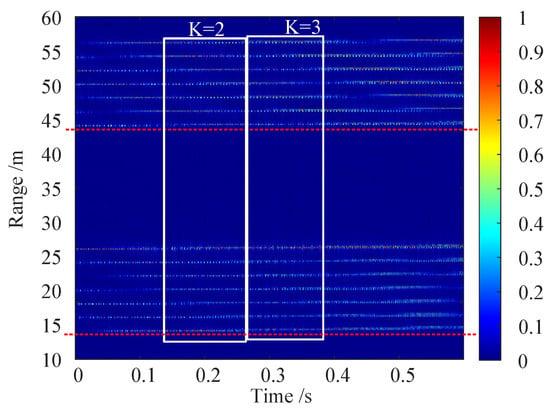
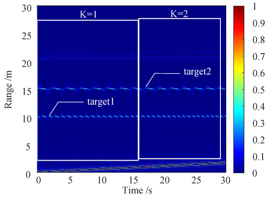
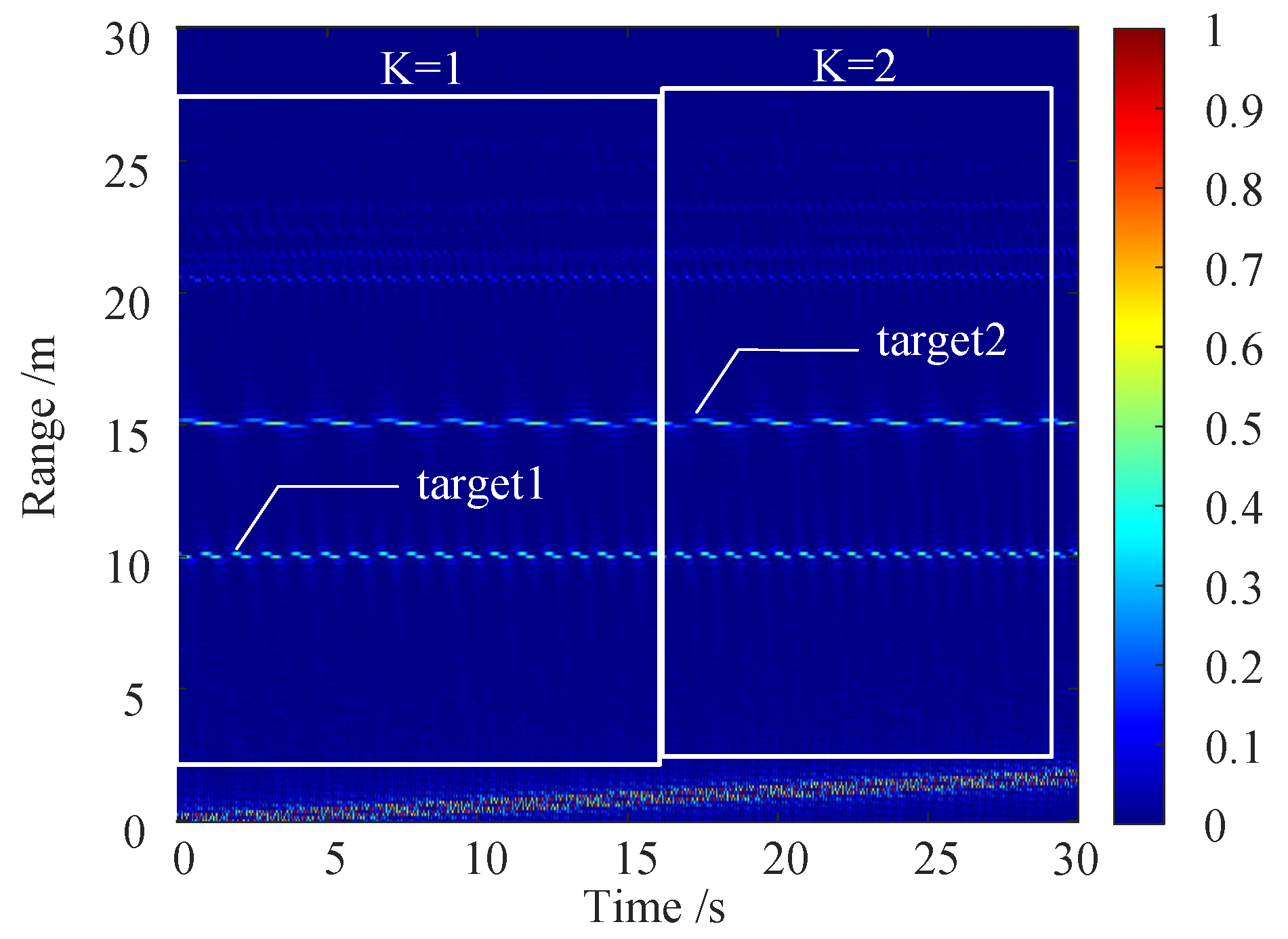
A total of 658 effective echo pulses are acquired in practice. According to the adaptive criterion, the full aperture is divided into two segments with the single-side center of the imaging scene as the reference point: the first segment contains 323 pulses, and the second segment contains 298 pulses, corresponding to accumulation times of 16.15 s and 14.90 s, respectively. The remaining 37 pulses are discarded, as shown in Figure 12.

Figure 12. Time–range image before segmentation.

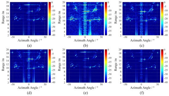
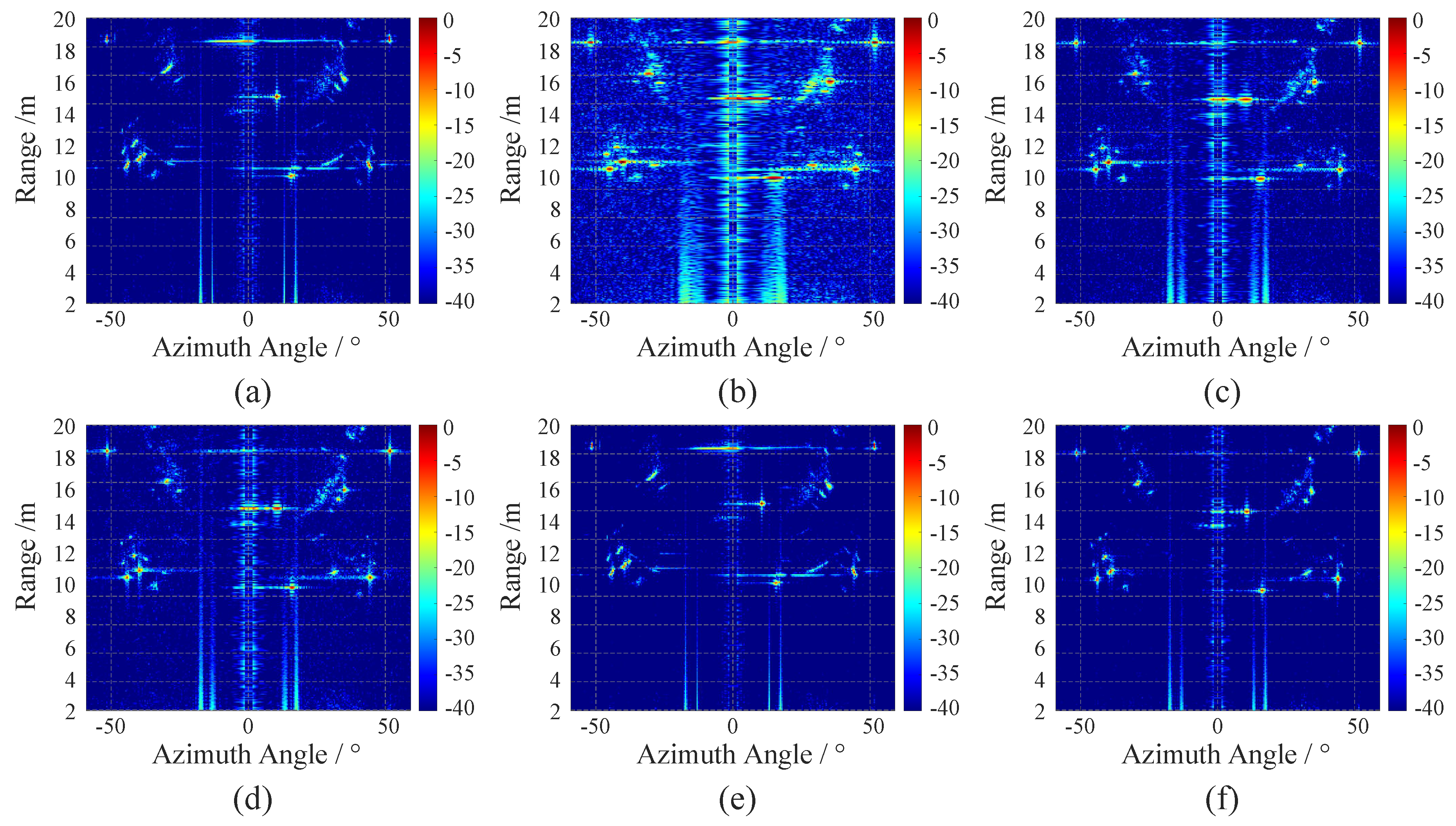
Figure 13 compares six processing schemes. In the full-aperture direct imaging result in Figure 13a, the target energy is severely defocused. The uniform segmentation scheme with 100 pulses/segment Figure 13b avoids nonlinear accumulation but suffers from insufficient single-segment resolution, resulting in severe target broadening. The schemes with 200 pulses/segment in Figure 13c and 300 pulses/segment in Figure 13d show gradually improved resolution, yet they still exhibit noticeable sidelobe elevation. The global ADMM method in Figure 13e improves sidelobe suppression, but its defocusing mitigation is limited. In contrast, with the proposed method in Figure 13f, both corner reflectors are clearly focused, the target center positions are consistent with the preset values, and the background energy is the lowest.

Figure 13. Imaging results of different methods. (a) Full-aperture direct imaging. (b) Uniform-segment compensation: 100 echoes per segment. (c) Uniform-segment compensation: 200 echoes per segment. (d) Uniform-segment compensation: 300 echoes per segment. (e) Alternating Direction Method of Multipliers (ADMM)-based compensation. (f) The proposed adaptive-segment compensation method.

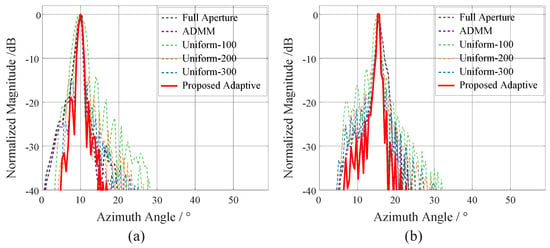
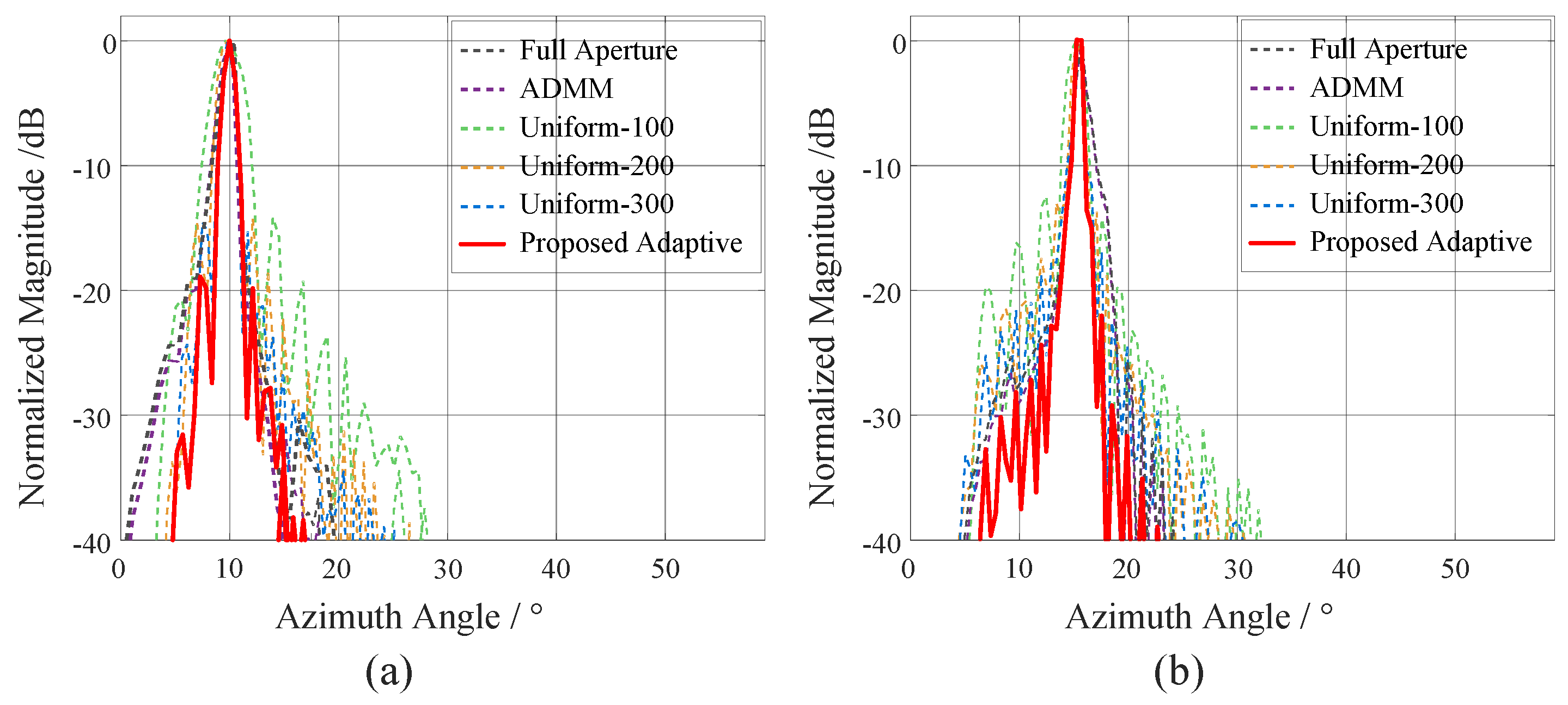
Figure 14 shows the azimuth-direction point-spread functions (PSF) of the two targets under five different processing schemes. Combining image entropy and PSF metrics, this paper comprehensively evaluates the measured imaging performance from two dimensions: the statistical characteristics of global energy distribution and the spatial-domain resolution details. Quantitative statistical results demonstrate that the image entropy values corresponding to full-aperture direct imaging, global ADMM compensation, and the proposed adaptive segmentation method are $4.8288$, $4.7075$, and $4.6970$, respectively. Compared with full-aperture imaging, global ADMM compensation reduces image entropy by approximately $2.5\%$, while the proposed method achieves a reduction of about $2.7\%$. The entropy improvement of both methods in the measured scenario is significantly lower than that in simulation scenarios. The primary reason lies in the limitation of the effective travel range of the rail platform: the measured aperture can only be divided into two sub-apertures, so the dynamic segment-length optimization advantage of the adaptive segmentation algorithm for long apertures with multiple segments cannot be fully exploited. In terms of the detailed performance of azimuth-direction PSF, the PSF obtained by the proposed method features a narrower mainlobe width and better sidelobe suppression. It outperforms the global ADMM scheme distinctly in target-edge sharpness and spatial resolution capability, and it can distinguish the boundaries of adjacent targets more clearly.

Figure 14. Point-Spread Functions (PSFs) of the measured point targets. (a) Target 1. (b) Target 2.

5. Discussion

This paper has proposed an adaptive segmentation and cross-segment coherent reconstruction algorithm based on phase error constraints for the nonlinear Doppler mismatch problem in long-aperture forward-looking radar imaging of high-maneuver platforms. The algorithm consists of two coupled stages. In the segmentation stage, a second-order residual phase error constraint is established based on the Rayleigh criterion, yielding an explicit adaptive criterion for sub-aperture duration that ensures the signal in each segment satisfies the local quasi-linear condition. In the reconstruction stage, the inter-segment compensation is modeled as a two-dimensional operator separable in the range and azimuth directions, and the ADMM is introduced for iterative solution, achieving phase alignment and coherent focusing across multiple sub-apertures.

Simulations and measured data validate the effectiveness of the proposed method. In point-target simulations, imaging metrics including peak sidelobe ratio, integrated sidelobe ratio, full-width-half-maximum and energy concentration are compared among different processing approaches. The results demonstrate that the proposed adaptive-segmentation combined with cross-sub-aperture coherent reconstruction achieves comprehensive advantages in azimuth resolution and energy-focusing performance. Compared with the global ADMM compensation without sub-aperture processing, our method increases the energy concentration from $0.15$ to $0.18$, corresponding to a $20\%$ improvement. The full-width-half-maximum decreases from $3.49$ to $3.00$, yielding approximately $14\%$ enhancement in azimuth resolution, while sidelobe metrics are also slightly optimized. It indicates that the two-stage framework of “adaptive sub-aperture partitioning + cross-sub-aperture coherent reconstruction” can effectively mitigate defocusing caused by phase nonlinearity over long apertures, and outperforms the single-stage global compensation in both resolution and energy focusing. Fixed-length segmentation schemes suffer from an inherent trade-off between azimuth resolution and energy concentration: shorter segments provide better resolution but suffer from energy dispersion and degraded sidelobes, whereas longer segments achieve higher energy concentration at the cost of reduced resolution. Our proposed method effectively breaks this trade-off. It achieves approximately $29\%$ improvement in energy concentration while maintaining the high resolution identical to the 300-pulse fixed-length scheme. Compared with the 600-pulse fixed-length scheme of similar energy level, our method exhibits remarkable resolution superiority. This benefit originates from the adaptive segmentation strategy, which dynamically adjusts segment length according to local phase nonlinearity and avoids over-segmentation in linear regions as well as insufficient segmentation in nonlinear regions. Furthermore, compared with the result of a single sub-aperture using adaptive segmentation, the cross-sub-aperture coherent reconstruction substantially improves sidelobe performance and energy concentration without resolution loss, which further verifies the effectiveness of the ADMM-based cross-segment phase-alignment strategy.

It should be acknowledged that there exist several limitations in the present work. First, the adaptive segmentation criterion is derived under the assumption of uniform linear motion. Its extension to scenarios with non-uniform velocity trajectories and curved flight paths deserves further investigation. Second, the ADMM-based optimization introduces additional computational overhead compared with the single-pass compensation approach, and the real-time implementation remains an unsolved issue. Future work will focus on extending the algorithm to more complex motion models, reducing computational cost via deep unfolding techniques, and validating the method on an airborne forward-looking SAR platform to improve its engineering practicality. Meanwhile, mature engineering measures including multi-core parallel computing, offline pre-computation of operators and embedded-hardware porting will be adopted to promote the real-time deployment and practical-scene application of the algorithm.

References

- Ding, T.; Song, Y.; Xu, Z.; Wang, Y.; Jin, T. A Chebyshev Inclusion Function-Based Pattern Evaluation Method for Phased Array under Multi-dimensional Elements Position Errors. IEEE Trans. Antennas Propag. 2026, 74, 1521–1534. [Google Scholar] [CrossRef] [Scilit]
- Shen, S.; Niu, X.; Guo, J.; Zhang, Z.; Han, S. High-Resolution Collaborative Forward-Looking Imaging Using Distributed MIMO Arrays. Remote Sens. 2024, 16, 3991. [Google Scholar] [CrossRef] [Scilit]
- Wei, D.; Chen, W.; Cheng, J. Terrain following based on forward-looking image sequences for unmanned air vehicles. Hongwai Yu Jiguang Gongcheng Infrared Laser Eng. 2017, 46, 428002. [Google Scholar] [CrossRef] [Scilit]
- Ouchi, K. Recent Trend and Advance of Synthetic Aperture Radar with Selected Topics. Remote Sens. 2013, 5, 716–807. [Google Scholar] [CrossRef] [Scilit]
- Zeng, T.; Wang, Z.; Wang, F.L.C. An Improved Frequency-Domain Image Formation Algorithm for Mini-UAV-Based Forward-Looking Spotlight BiSAR Systems. Remote Sens. 2020, 12, 2680. [Google Scholar] [CrossRef] [Scilit]
- Li, W.; Chen, R.; Yang, J.; Wu, J.; Huang, Y. Multichannel Radar Forward-Looking Imaging: Potential and Challenges. In Proceedings of the IGARSS 2023—2023 IEEE International Geoscience and Remote Sensing Symposium, Pasadena, CA, USA, 16–21 July 2023. [Google Scholar]
- Zheng, Z.; Tan, G.; Jiang, D. A Bidirectional Resampling Imaging Algorithm for High Maneuvering Bistatic Forward-Looking SAR Based on Chebyshev Orthogonal Decomposition. IEEE Trans. Geosci. Remote Sens. 2024, 62, 5211512. [Google Scholar] [CrossRef] [Scilit]
- Krieger, G.; Mittermayer, J.; Buckreuss, S.; Wendler, M.; Sutor, T.; Witte, F.; Moreira, A. Sector imaging radar for enhanced vision. Aerosp. Sci. Technol. 2003, 7, 147–158. [Google Scholar] [CrossRef] [Scilit]
- Cheng, C.; Gao, M.; Zhou, X. High-resolution forward-looking imaging algorithm for missile-borne detectors. J. Syst. Eng. Electron. 2019, 30, 456–466. [Google Scholar] [CrossRef] [Scilit]
- Chen, X.; Dong, Z.; Zhang, Z.; Tu, C.; Yi, T.; He, Z. Very High Resolution Synthetic Aperture Radar Systems and Imaging: A Review. IEEE J. Sel. Top. Appl. Earth Obs. Remote Sens. 2024, 17, 7104–7123. [Google Scholar] [CrossRef] [Scilit]
- Pu, W.; Wu, J.; Huang, Y.; Wang, X.; Yang, J.; Li, W.; Yang, H. Nonsystematic Range Cell Migration Analysis and Autofocus Correction for Bistatic Forward-looking SAR. IEEE Trans. Geosci. Remote Sens. 2018, 56, 6556–6570. [Google Scholar] [CrossRef] [Scilit]
- Ren, Y.; Tang, S.; Guo, P.; Zhang, L.; So, H.C. 2-D Spatially Variant Motion Error Compensation for High-Resolution Airborne SAR Based on Range-Doppler Expansion Approach. IEEE Trans. Geosci. Remote Sens. 2021, 60, 5201413. [Google Scholar] [CrossRef] [Scilit]
- José-Tomás, G.P.; Pablo, A.G.; Mateo, B.G.; Blas-Pablo, D.N. SAR System for UAV Operation with Motion Error Compensation beyond the Resolution Cell. Sensors 2008, 8, 3384–3405. [Google Scholar] [CrossRef] [Scilit] [PubMed]
- Hu, R.; Rao, B.S.M.R.; Murtada, A.; Alaee-Kerahroodi, M.; Ottersten, B. Automotive Squint-Forward-Looking SAR: High Resolution and Early Warning. IEEE J. Sel. Top. Signal Process. 2021, 15, 904–912. [Google Scholar] [CrossRef] [Scilit]
- Moreira, A. Real-time synthetic aperture radar (SAR) processing with a new subaperture approach. IEEE Trans. Geosci. Remote Sens. 1992, 30, 714–722. [Google Scholar] [CrossRef] [Scilit]
- Luo, J.; Huang, Y.; Mao, D.; Zhang, Y.; Zhang, Y.; Yang, J. Azimuth–Elevation Forward-Looking Super-Resolution Imaging Based on Sparse Doppler Phase Convolution Model for High-Speed Platform. IEEE Trans. Geosci. Remote Sens. 2024, 62, 5110118. [Google Scholar] [CrossRef] [Scilit]
- Wahl, D.E.; Eichel, P.H.; Ghiglia, D.C.; Jakowatz, C.V. Phase gradient autofocus—A robust tool for high resolution SAR phase correction. IEEE Trans. Aerosp. Electron. Syst. 1994, 30, 827–835. [Google Scholar] [CrossRef] [Scilit]
- Xing, M.; Lin, H.; Chen, J.; Sun, G.; Yan, B. A Review of Imaging Algorithms in Multi-platform-borne Synthetic Aperture Radar. J. Radars 2019, 8, 732–757. [Google Scholar]
- Morrison, R.L.; Do, M.N.; Munson, D.C. SAR image autofocus by sharpness optimization: A theoretical study. IEEE Trans. Image Process. 2007, 16, 2309–2321. [Google Scholar] [CrossRef] [Scilit] [PubMed]
- Seo, K.; Kwon, Y.; Kim, C.K. An Enhanced Phase Gradient Autofocus Algorithm for SAR: A Fractional Fourier Transform Approach. Remote Sens. 2025, 17, 1216. [Google Scholar] [CrossRef] [Scilit]
- Luo, C.; Liang, Y.; Gao, J.; Lei, G.; Han, C. A Scene-Adaptive Phase Gradient Autofocus Algorithm. Remote Sens. 2025, 17, 260. [Google Scholar] [CrossRef] [Scilit]
- Zhang, L.; Qiao, Z.; Xing, M.D.; Yang, L.; Bao, Z. A Robust Motion Compensation Approach for UAV SAR Imagery. IEEE Trans. Geosci. Remote Sens. 2012, 50, 3202–3218. [Google Scholar] [CrossRef] [Scilit]
- Zhu, D.; Jiang, R.; Mao, X.; Zhu, Z. Multi-Subaperture PGA for SAR Autofocusing. IEEE Trans. Aerosp. Electron. Syst. 2013, 49, 468–488. [Google Scholar] [CrossRef] [Scilit]
- Zhang, Y.; Huang, L.; Xu, Z.; Wang, Z.; Chen, B. Combined Motion Compensation Method for Long Synthetic Aperture Radar Based on Subaperture Processing. J. Mar. Sci. Eng. 2025, 13, 355. [Google Scholar] [CrossRef] [Scilit]
- Fornaro, G. Trajectory deviations in airborne SAR: Analysis and compensation. IEEE Trans. Aerosp. Electron. Syst. 1999, 35, 997–1009. [Google Scholar] [CrossRef] [Scilit]
- Rufenach, C.; Alpers, W. Imaging ocean waves by synthetic aperture radars with long integration times. IEEE Trans. Antennas Propag. 1981, 29, 422–428. [Google Scholar] [CrossRef]
- Mao, D.; Tuo, X.; Luo, J.; Zhang, P.; Zhang, Y.; Zhang, Y.; Huang, Y.; Yang, J. Scanning Radar Forward-Looking Imaging Under High-Speed Platform by Accurate Profile-Phase Deconvolution Method. IEEE Trans. Geosci. Remote Sens. 2024, 62, 5107613. [Google Scholar] [CrossRef] [Scilit]
- Li, H.; Cao, R.; Yang, T.; Lu, P.; Nan, Y.; Wang, R. Fine-Resolution Spaceborne Radar Imaging of Space Targets with Parametric Second-Order Scaling and High-Order Spatial-Variant Phase Compensation. IEEE J. Sel. Top. Appl. Earth Obs. Remote Sens. 2025, 18, 17281–17296. [Google Scholar] [CrossRef] [Scilit]
- Wang, X.; Lu, J.; Meng, Z.; Zhang, L. Forward-looking multi-channel synthetic aperture radar imaging and array attitude error compensation. J. Radars 2023, 12, 1155–1165. [Google Scholar] [CrossRef]
- Mizuno, S. Synthetic Aperture Radar Signal Processing System; Wiley: New York, NY, USA, 1999. [Google Scholar]
Disclaimer/Publisher’s Note: The statements, opinions and data contained in all publications are solely those of the individual author(s) and contributor(s) and not of MDPI and/or the editor(s). MDPI and/or the editor(s) disclaim responsibility for any injury to people or property resulting from any ideas, methods, instructions or products referred to in the content. |
© 2026 by the authors. Licensee MDPI, Basel, Switzerland. This article is an open access article distributed under the terms and conditions of the Creative Commons Attribution (CC BY) license.