PFIRNet: UAV-to-Satellite Cross-View Self-Localization via Continuous Probability Field Inference

Highlights

What are the main findings?

• PFIRNet reformulates UAV-to-satellite self-localization from discrete satellite tile retrieval into continuous coordinate-space posterior inference.
• On DenseUAV, PFIRNet reduces the median localization error to 9.84 m and remains robust in sparse and non-aligned satellite galleries.

What are the implications of the main findings?

• Continuous probability field inference provides a more reliable localization readout than top-1 tile-center selection.
• The method improves deployment adaptability for GNSS-degraded UAV localization without relying on denser satellite galleries or costly post-retrieval matching.

Abstract

UAV (Unmanned Aerial Vehicle)-to-satellite self-localization is commonly treated as satellite tile retrieval. This makes large-area search tractable, but it also forces a continuous localization problem into a discrete ranking form. Once the task is defined this way, training naturally relies on hard positive–negative tile labels, and inference tends to read coordinates from the top-ranked tile center. The model, therefore, learns image identity more than geographic continuity, while the final estimate remains vulnerable to tile-center quantization and top-1 retrieval errors. We propose PFIRNet (Probability Field Inference Network), a continuous geographic posterior inference framework that reformulates retrieval outputs as evidence for coordinate estimation rather than discrete tile selection. It uses distance-aware geographic supervision to shape candidate responses according to metric proximity, lifts top-k candidates into a coordinate-space probability field, and applies risk-calibrated multi-peak verification to update the estimate only when an alternative posterior peak is sufficiently supported. On DenseUAV, PFIRNet reduces the median localization error to 9.84 m and outperforms both one-stage retrieval methods and two-stage matching baselines. It also remains more robust under sparse and non-aligned satellite galleries.

1. Introduction

UAV self-localization aims to recover the platform location in geographic space from onboard visual observations. It is a key capability for autonomous navigation, emergency inspection, low-altitude remote sensing, and spatial situational awareness in GNSS-denied or GNSS-degraded environments. Existing studies on UAV-to-satellite cross-view localization have mainly followed a retrieval-based framework. Given a UAV query image, the model retrieves the most visually similar reference tile from a geo-tagged satellite reference gallery and uses the tile coordinate as the localization result. Early work on wide-area image geo-localization showed that ground-view or low-altitude images can establish large-scale visual correspondences with aerial reference images [1]. Later, UAV multi-view benchmarks, local pattern modeling, and Transformer-based representations further advanced repeatable evaluation and structural matching among UAV, satellite, and ground-view images [2,3,4]. In settings closer to low-altitude urban remote sensing, datasets and methods such as DenseUAV also showed that a dense reference gallery can substantially improve candidate-region recall [5,6,7]. These studies provide an effective large-scale search basis for UAV remote-sensing self-localization. However, the final localization result still usually depends on the ranking and coordinate readout of discrete reference tiles.

This discretization assumption limits the expressive capacity of retrieval-based self-localization in real remote-sensing scenarios. The true UAV location lies in continuous geographic space, whereas the satellite reference gallery is only a finite sampling of the continuous remote-sensing base map. Even when the top-ranked tile comes from the correct region, its center coordinate may not match the true UAV location. This discrete-anchor error becomes larger when the gallery is sparse, when the query lies near a tile boundary, or when the reference gallery is not strictly aligned with the query trajectory. Increasing gallery density can alleviate this problem, but it also increases storage, retrieval, and update costs. Therefore, UAV self-localization requires more than merely accurate tile ranking. It also needs a mechanism that converts discrete remote-sensing candidate evidence into continuous coordinate inference.

Hard positive–negative assignment in training further aggravates this problem. Mainstream retrieval training usually treats the strictly corresponding satellite tile as the only positive sample and all other tiles as negative samples. This one-hot supervision facilitates retrieval representation learning, but it ignores the spatial coverage of remote-sensing images and the continuity of geographic space. Hard negative sampling has shown that candidate selection can strongly affect cross-view representation learning [8]. Non-one-to-one retrieval settings also suggest that a query image may not strictly coincide with the center of any reference image [9]. Under hard positive–negative assignment, geographically nearby candidates and distant candidates are both treated as negative samples. This weakens the model’s ability to learn the continuous correspondence between candidate similarity and true geographic proximity.

Another line of work introduces fine-grained localization or image registration after retrieval to overcome the precision limit of tile-center coordinates. Correlation-aware homography estimation, coarse-to-fine offset estimation, and region-to-point localization show that local geometric alignment can further refine coordinates when the candidate region covers the true location [10,11,12]. However, these methods usually depend on the candidate region provided by the retrieval stage. Once the top-ranked tile falls in an incorrect region, the subsequent registration step can only optimize within the wrong spatial support. Sequentially testing multiple candidates also introduces extra computation and increases the risk of erroneous switching. Thus, the key limitation of post-retrieval refinement is the lack of a structured representation of candidate uncertainty.

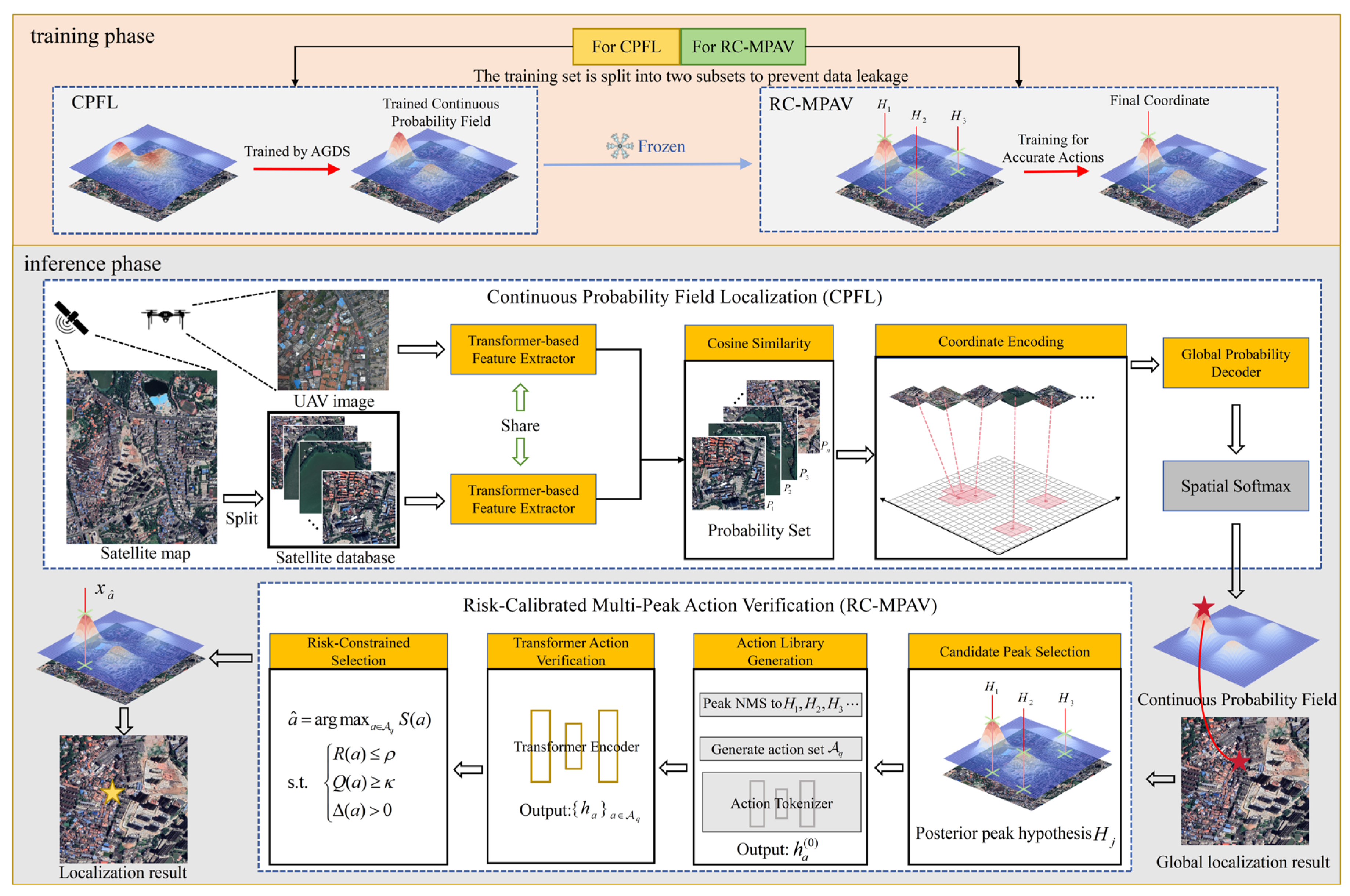
Based on these observations, we propose PFIRNet, which reorganizes UAV-to-satellite self-localization from discrete gallery retrieval into continuous geographic posterior inference driven by cross-source remote-sensing matching evidence. PFIRNet treats satellite tiles as discrete support points in continuous geographic space rather than final class labels. It also treats UAV-satellite similarity as observational evidence for the location posterior rather than only as a ranking score. Specifically, PFIRNet first uses Adaptive Geographic Distribution Supervision (AGDS) to convert the metric distance between each candidate and the true location into soft geographic supervision. This encourages cross-source representation learning to preserve geographic–topology consistency. PFIRNet then lifts candidate similarities and coordinates into a continuous probability field, so the localization estimate is no longer restricted to a single tile center. Finally, PFIRNet performs risk-calibrated action verification over multiple local posterior peaks. It makes a constrained localization decision among retaining the current estimate, local posterior readout, and alternative-peak switching.

The main contributions of this study are as follows:

• We propose PFIRNet, a continuous probability field inference framework for UAV remote-sensing self-localization. It lifts tile-level retrieval into coordinate-space posterior estimation for cross-source remote-sensing image matching.
• We propose Adaptive Geographic Distribution Supervision (AGDS). It replaces hard one-hot labels with a distance-aware soft geographic distribution, enabling the model to learn the continuous correspondence between candidate responses and true geographic proximity.
• We propose Continuous Probability Field Localization (CPFL). It lifts the similarities and coordinates of top-k remote-sensing candidates into a continuous geographic probability field, supporting sub-tile coordinate readout and multimodal uncertainty representation.
• We propose Risk-Calibrated Multi-Peak Action Verification (RC-MPAV). It addresses decision risk in multimodal posteriors by calibrating the selection among retaining the current estimate, local posterior readout, and alternative-peak switching, thereby improving the reliability of localization decisions.

2. Related Work

To clarify the conceptual position of PFIRNet, we organize related studies into three aspects, retrieval-based cross-view geo-localization, geography-aware supervision for spatially structured representation learning, and fine-grained localization with post-retrieval refinement. These approaches share the use of cross-source visual correspondence and candidate-region retrieval as the basis for localization, but they differ in how geographic relationships are supervised, how coordinates are read out, and how uncertainty is handled after retrieval. As summarized in

Table 1. Conceptual comparison between existing localization methods and PFIRNet.

Key Aspect	Existing Localization Methods	PFIRNet
Geographic supervision	Mostly uses hard positive–negative labels or identity-level objectives. Nearby candidates may still be treated as negative samples.	Uses Adaptive Geographic Distribution Supervision to represent metric proximity with a distance-aware soft geographic distribution
Coordinate readout	Usually returns the center or predefined coordinate of the top-ranked tile. Some methods average multiple candidates, but the output remains tied to discrete gallery anchors.	Uses Continuous Probability Field Localization to transform top-k candidate responses into a continuous coordinate-space posterior.
Post-retrieval correction	Applies local matching, registration, or offset estimation within selected candidate regions. The correction usually depends on the reliability of the retrieved region.	Uses Risk-Calibrated Multi-Peak Action Verification to compare the default readout with alternative posterior peaks before switching.

, PFIRNet retains the candidate recall role of retrieval-based localization while reformulating candidate responses as evidence for continuous coordinate inference.

2.1. Retrieval-Based Cross-View Geo-Localization

Cross-view geo-localization has long been formulated mainly as an image retrieval problem. Given a query image from a ground, UAV, or aerial platform, the model retrieves the most similar image from a geo-tagged satellite or aerial reference gallery and uses the reference coordinate as the localization output. Early work on wide-area image geo-localization demonstrated the feasibility of large-scale matching between ground-view images and aerial reference images [1]. CVM-Net then learned shared representations between ground-view and aerial images through a two-branch deep network [13]. SAFA further improved structural correspondence across views through spatial-aware feature aggregation [14]. These methods established the basic paradigm of cross-view visual geo-localization. They convert spatial localization into reference gallery ranking by learning view-invariant representations.

Within this paradigm, orientation and spatial structure have gradually become important cues. Lending Orientation to Neural Networks introduced orientation priors into cross-view matching and reduced the orientation gap between ground-view and overhead images [15]. For UAV platforms, University-1652 provided a multi-view benchmark covering UAV, satellite, and ground-view images, making UAV-to-satellite retrieval a standard task for repeatable evaluation [2]. LPN used local pattern modeling to highlight the importance of region-level details in UAV-satellite matching [3]. TransGeo used Transformers to model global dependencies and positional relationships [4]. These studies show that cross-view localization cannot rely only on whole-image appearance similarity. It also needs local structure, orientation relationships, and long-range spatial dependencies.

As the demand for UAV remote-sensing self-localization has increased, recent studies have further focused on low-altitude, multi-altitude, and large-scale urban environments. DenseUAV advanced the task toward low-altitude urban UAV self-localization by introducing denser satellite references and localization-oriented evaluation [5]. SUES-200 extended UAV-to-satellite benchmarks from the perspective of altitude and scene variation [16]. UAV-VisLoc provided large-scale UAV visual localization data for more realistic evaluation [17]. Meanwhile, MCCG used ConvNeXt and multiple classifiers to enhance discriminative features [18]. Multi-branch joint representation learning combined global and local cues through information fusion [19]. MEAN improved alignment through multi-level embedding and consistency constraints [20]. CV-Cities further extended cross-view localization to larger-scale city-level generalization scenarios [21]. More general place recognition and cross-view retrieval methods also improve robustness under changing environments, viewpoints, weather, or modalities [22,23,24,25,26]. These methods substantially improve the matching ability between UAV and satellite images, but their outputs are still usually reference tile rankings.

Overall, existing retrieval-based methods can provide effective candidate-region recall for UAV-to-satellite localization. However, the final position readout usually depends on discrete tile centers or predefined annotation coordinates. Because the reference gallery is only a finite sampling of continuous geographic space, recalling the correct region does not necessarily imply coordinate accuracy. If the UAV field of view is not strictly aligned with the satellite tile, or if the gallery sampling density is insufficient, the tile center itself can become an additional source of error. How to convert retrieval evidence from multiple candidates into a continuous coordinate estimate remains a key problem for retrieval-based frameworks.

2.2. Geography-Aware Supervision for Spatially Structured Representation Learning

Beyond network architecture, the supervision strategy determines whether cross-view representations can preserve geographic spatial structure. Traditional retrieval training usually relies on classification, contrastive learning, or triplet loss. These objectives pull cross-view images with the same location identity closer in the embedding space and push images with different identities apart. Sample4Geo strengthened the model’s ability to distinguish hard candidates through hard negative sampling, showing that the sampling strategy can strongly affect cross-view representation learning [8]. Such methods improve retrieval discriminability, but they usually treat geographically nearby candidates as harder negative samples rather than spatial support related to the true location.

Recent methods have increasingly introduced spatial, geometric, or scene consistency explicitly. ConGeo performs robust cross-view contrastive learning under ground-view variations, emphasizing the importance of representation stability under viewpoint perturbations [27]. GeoDTR and its follow-up work learn cross-view structural correspondence through geometric layout decoupling, so the model no longer depends only on appearance texture [28,29]. Domain alignment and scene consistency methods further address cross-domain appearance differences and scene-level consistency [30]. GeoSSK enhances cross-view correspondence from the perspectives of local semantic similarity and knowledge distillation [31]. Together, these studies show that cross-view geo-localization should exploit spatial structure rather than only optimizing global image similarity.

However, using spatial structure does not mean that the supervision target has become continuous. In many methods, geographic or semantic information is mainly used to build stronger representations, select harder samples, or enhance cross-domain consistency. The final training objective still serves discrete image-identity discrimination. VIGOR challenged the strict one-to-one retrieval assumption and showed that a query image does not necessarily correspond exactly to the center of a reference image [9]. UCVGL and unsupervised coarse-to-fine methods further indicate that precise cross-view pair annotations are costly in large-scale scenarios, making weakly supervised or unsupervised signals practically valuable [32,33]. GeoCLIP also represents geographic locations in a learnable coordinate-aware embedding space [34]. These studies move the task setting closer to real scenarios, but the metric distance between each candidate and the true location is usually not directly organized into a candidate-level supervision distribution.

For UAV self-localization, the key question is not only how to obtain stronger cross-view representations. It is also how to make model responses consistent with true geographic distance. Existing geographic-aware supervision usually uses spatial structure to enhance feature discriminability, but the metric distance between candidates is still rarely modeled directly as a supervision distribution. As a result, the model can learn to distinguish different image identities, but it may not learn how candidate similarity should vary continuously with spatial proximity. A candidate-level supervision mechanism is, therefore, still needed to explicitly connect metric distance, retrieval response, and subsequent coordinate inference.

2.3. Fine-Grained Localization and Post-Retrieval Refinement

Tile-level retrieval is insufficient for fine-grained self-localization. Many studies, therefore, introduce local refinement or image registration after initial retrieval. The correlation-aware homography estimator estimates local geometric transformations through correlation modeling for fine-grained cross-view localization [10]. OS-FPI adopts a coarse-to-fine one-stream framework for response or offset estimation in UAV geo-localization [11]. R2PLoc formulates UAV visual geo-localization as a region-to-point problem and combines coarse region retrieval with hierarchical semantic keypoint refinement [12]. Two-stage frameworks such as GRiM-Net also aim to connect region-level recall with point-level localization [35]. These studies show that returning a single satellite tile is not sufficient for accurate UAV self-localization. The localization system must further infer the position inside the candidate region.

More general image matching and remote-sensing image registration methods provide technical foundations for this direction. SuperGlue uses graph neural networks for local feature matching [36]. LoFTR establishes dense or semi-dense correspondences through detector-free Transformers [37]. ASpanFormer improves correspondence modeling in complex regions with adaptive span Transformers [38]. LightGlue emphasizes efficient local matching [39], and RoMa further advances robust dense matching [40]. In remote sensing, SwinMatcher models interactive feature correspondences for cross-modal remote-sensing image matching [41]. LiteSAM focuses on lightweight and robust matching between satellite and aerial images [42]. These methods can provide strong tools for local registration when candidate images cover the same physical region.

The problem is that post-retrieval refinement often assumes that the candidate region is already reliable. If the top-ranked tile from the retrieval stage comes from an incorrect region, local feature matching, homography estimation, or offset regression can only search for an optimum within the wrong spatial support. Recent studies have begun to address more complex non-aligned aerial satellite views and unified UAV cross-view localization. Beyond Matching to Tiles focuses on visual navigation under non-aligned aerial satellite views [43]. Three-dimensional (3D) geometric perception methods attempt to unify coarse retrieval and fine-grained pose estimation [44]. UAV pose estimation with satellite imagery also reflects an early shift from image retrieval toward pose inference [45]. These studies suggest that the field is moving from discrete matching toward structured spatial inference.

Nevertheless, existing retrieval-then-refinement pipelines still lack a sufficient representation of candidate uncertainty. Sequentially testing multiple top-k candidates can reduce the risk caused by a top-1 error, but it treats candidates as independent matching attempts and increases online computational costs. A local matcher itself also has limited ability to decide when to retain the current candidate, when to perform local posterior readout, and when to switch to another spatial hypothesis. Fine-grained UAV self-localization, therefore, needs a unified representation of multiple spatial hypotheses in addition to local registration capability.

3. Methodology

3.1. Overview of Our Method

Given a UAV query image $I_q$ and a geo-tagged satellite reference gallery $\mathcal{G}={\{(I_i^s,c_i)\}}_{i=1}^N$, $I_i^s$ and $c_i$ denote the $i$-th satellite tile and its center coordinate in a local metric coordinate system, respectively. Mainstream retrieval-based methods usually learn the similarity $s(I_q,I_i^s)$ between the query image and each reference tile. They then directly use the center of the highest-scoring tile as the localization result:

$$\widehat{i}=\arg {\max }_i s(I_q,I_i^s),\hspace{1em}\widehat{x}=c_{\widehat{i}}$$

(1)

This readout strategy is suitable for large-scale candidate recall. However, it simplifies continuous location estimation into the selection of a discrete tile center. It can, therefore, introduce anchor errors when the fields of view are not aligned or when the gallery sampling is insufficient.

Based on this observation, PFIRNet retains the candidate recall capability of the retrieval framework but redefines its coordinate readout. Satellite tiles are no longer treated as mutually exclusive location classes. Instead, they are treated as discrete evidence support points in continuous geographic space. Accordingly, UAV-satellite similarity is no longer used only as a ranking score. It is organized as evidence for the continuous location posterior $P(x\mid I_q,\mathcal{G})$. Under this framework, multiple candidates jointly support a coordinate-space probability field. The localization estimate can then be read out from the posterior distribution, rather than being restricted to the center of a single reference tile.

As shown in Figure 1, PFIRNet consists of two connected stages: Continuous Probability Field Localization (CPFL) and Risk-Calibrated Multi-Peak Action Verification (RC-MPAV). CPFL converts cross-view retrieval evidence into a coordinate-space posterior. Following the DenseUAV baseline, we use its released Transformer-based two-branch backbone. First, the UAV query image and candidate satellite tiles are encoded by a two-branch feature network. Their similarities are then used to form probabilistic candidate responses. Next, the candidate responses and their geographic coordinates are jointly mapped into the local metric space to generate a global continuous probability field and an initial localization estimate. Based on this field, RC-MPAV further performs risk-calibrated readout over the multimodal posterior structure. During training, CPFL is frozen as a converged stage-one module, and RC-MPAV learns to choose among retaining the dominant posterior peak, local posterior readout, and alternative-peak switching. During inference, the system updates the localization estimate only when an alternative action has sufficient posterior support and controlled expected risk. Through this design, PFIRNet converts the traditional retrieval pipeline into a continuous localization process: it first constructs a field from candidate evidence and then selects reliable coordinates from the posterior field.

3.2. Adaptive Geographic Distribution Supervision

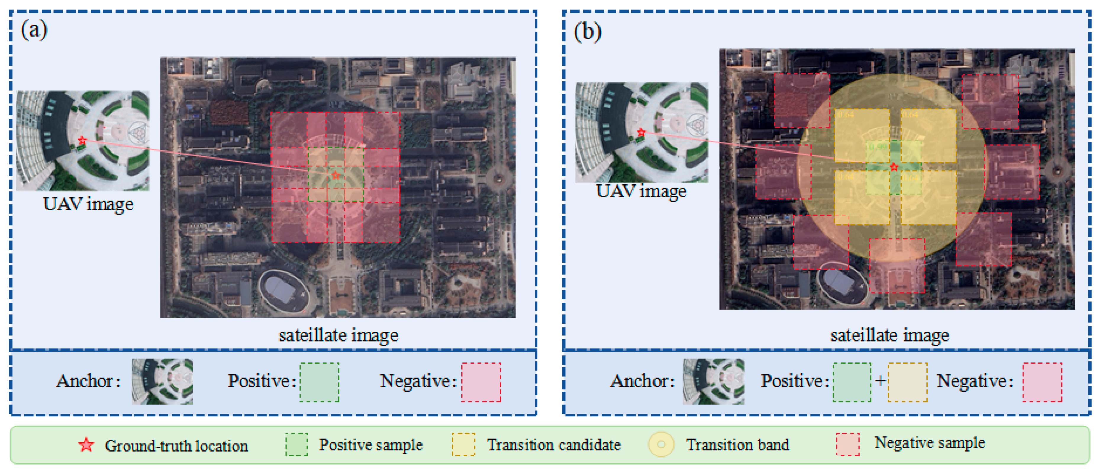
As shown in Figure 2a, traditional classification or triplet-based training usually treats the satellite tile nearest to the query location as the only positive sample. All remaining candidates are treated uniformly as negative samples. This hard assignment helps the model learn discrete identity discrimination, but it ignores the continuous geographic structure in UAV self-localization. Nearby tiles may still provide valid spatial support for the query location. Distant tiles should not receive the same supervision signal, even if they have similar visual appearance. To address this issue, Adaptive Geographic Distribution Supervision (AGDS) assigns geographic support weights according to the metric distance between each candidate center and the true location. It converts the original discrete positive–negative assignment into continuous candidate-level supervision.

As shown in Figure 2b, AGDS first adaptively partitions the candidate set according to the metric distance between the query ground-truth location and each candidate satellite center. Let the query ground-truth coordinate be $x_q$, and let the candidate center be $c_i$. Their distance is defined as $d_i=\Vert c_i-x_q{\Vert }_2$. Given an annealed geographic scale ${\sigma }_e$, which gradually decreases during training, the candidate set is divided into a core positive support, a transitional support, and a distant negative region:

$${\mathcal{P}}_q=\{i\mid d_i\le r_p{\sigma }_e\},\hspace{1em}{\mathcal{T}}_q=\{i\mid r_p{\sigma }_e<d_i<r_n{\sigma }_e\},\hspace{1em}{\mathcal{N}}_q=\{i\mid d_i\ge r_n{\sigma }_e\}$$

(2)

where ${\mathcal{P}}_q$ provides stable positive samples. ${\mathcal{T}}_q$ preserves the continuous support of geographically nearby candidates. ${\mathcal{N}}_q$ maintains the distant discriminative boundary. The parameters $r_p$ and $r_n$ control the radii of the positive support and the distant negative region, respectively. The scale ${\sigma }_e$ allows the model to learn cross-source spatial correspondence from a relatively wide neighborhood at the early training stage. As training proceeds, ${\sigma }_e$ gradually decreases, and the supervision range shrinks toward a finer localization neighborhood. This annealing process avoids prematurely treating nearby tiles as hard negative samples. It also reduces the risk of over-smoothing in the late stage of training.

The above partition defines the supervision role of each candidate in geographic space. However, the region partition alone cannot directly constrain the network output. To convert this spatial relationship into an optimizable objective, AGDS further represents the metric distance as a candidate-level soft geographic distribution:

$$y_i^{geo}={\displaystyle \frac{\exp (-d_i^2/(2{\sigma }_e^2))}{{\displaystyle \sum _j\exp }(-d_j^2/(2{\sigma }_e^2))+ϵ}}$$

(3)

where $y_i^{geo}$ denotes the geographic support weight of candidate $i$ for the query location, and $ϵ$ is used for numerical stability. Unlike standard label smoothing, this soft label does not assign a fixed probability to non-target classes. Instead, it is jointly determined by the true metric distance, the gallery sampling state, and the current training scale. In this way, AGDS can form a finer supervision distribution in dense galleries. It can also preserve necessary nearby support in sparse or non-aligned satellite galleries.

Let $w_i$ denote the normalized candidate weight output by the retrieval network. AGDS uses geographic soft classification loss to align model responses with the geographic support distribution:

$${\mathcal{L}}_{geo}=-{\displaystyle \sum _i{y}_i^{geo}}\log (w_i+ϵ)$$

(4)

where ${\mathcal{L}}_{geo}$ directly penalizes the model when it concentrates probability mass on locations far from the ground truth. At the same time, it allows nearby candidates to share the supervision. To preserve cross-region discriminability, AGDS also introduces a geographic soft triplet constraint. This constraint pulls the query feature closer to candidates in the core positive support and pushes it away from candidates in the distant negative region:

$${\mathcal{L}}_{tri}={\displaystyle \frac{1}{\left|{\mathcal{S}}_q\right|}}{\displaystyle \sum _{(i,j)\in {\mathcal{S}}_q}\log }\left(1+\exp \left(\alpha (D(q,i)-D(q,j))\right)\right)$$

(5)

where $D(q,i)$ denotes the distance between the UAV query feature and the feature of the $i$-th satellite candidate. The set ${\mathcal{S}}_q=\{(i,j)\mid i\in {\mathcal{P}}_q,j\in {\mathcal{N}}_q\}$ contains valid positive–negative candidate pairs, and $\alpha$ controls the strength of the ranking constraint.

3.3. Continuous Probability Field Localization

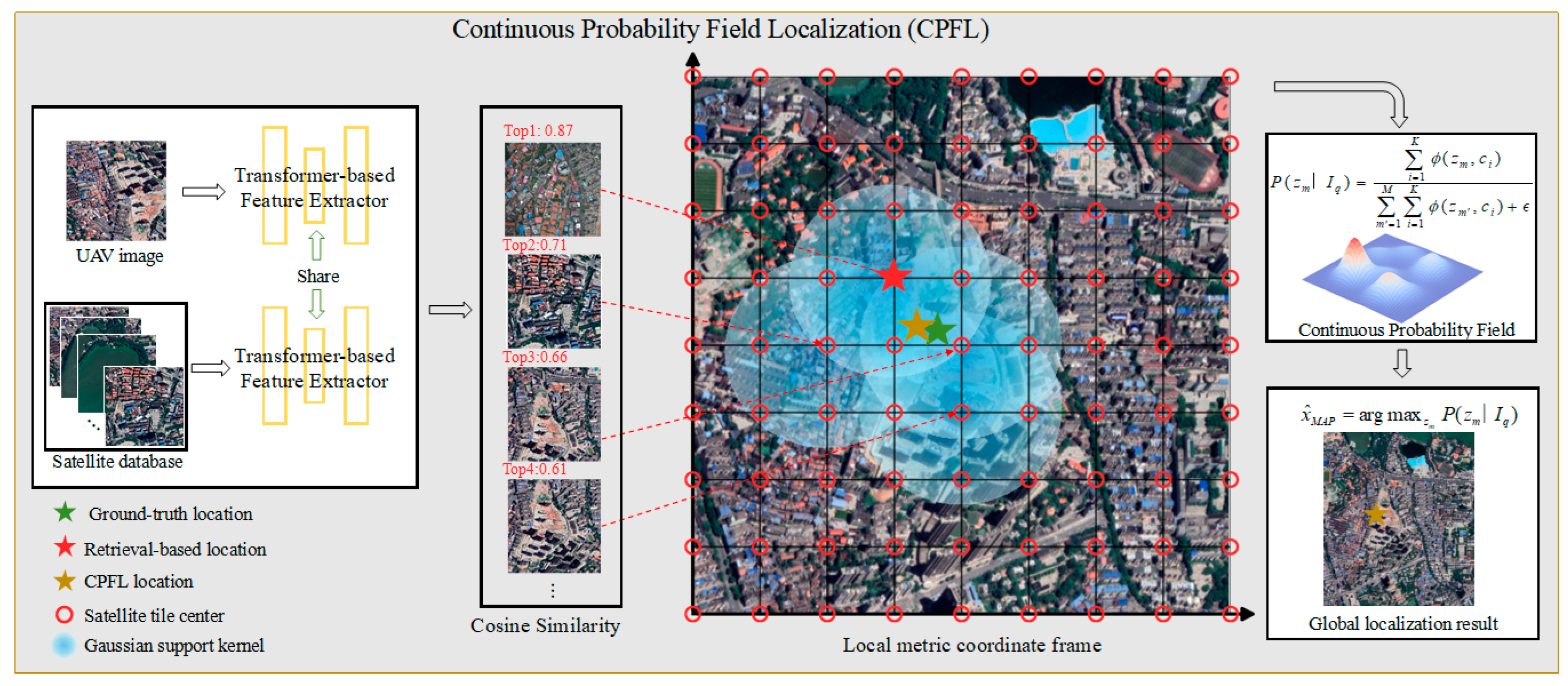
CPFL is the retrieval stage of PFIRNet. It converts discrete candidate evidence from retrieval into a coordinate-space posterior field. Unlike traditional methods that directly use the center of the top-1 satellite tile as the localization result, CPFL includes multiple high-response candidates in the localization readout. These candidates provide discrete spatial support points, while their retrieval responses provide candidate-level evidence. CPFL then lifts this candidate-level evidence into a local metric coordinate space by placing a Gaussian support kernel at each retrieved candidate center and superposing the weighted kernels. In this way, the retrieval stage can output a coordinate estimate that is not restricted to a single satellite tile center. It also generates a probability field that describes spatial support and multimodal uncertainty, which provides input for the risk-calibrated readout in RC-MPAV.

As shown in Figure 3, given a UAV query image $I_q$ and a candidate satellite image $I_i^s$, a two-branch backbone extracts the query feature and the satellite feature, respectively:

$$\left\{\begin{array}{l}{f}_q=F_u(I_q)\\ f_i=F_s(I_i^s)\end{array}\right.$$

(6)

where $F_u$ and $F_s$ denote the UAV branch and the satellite branch, respectively. They can share or partially share the backbone structure. $f_q$ and $f_i$ are normalized cross-view representations. The candidate similarity is computed by the feature inner product and is converted into a candidate-level probability mass through temperature softmax:

$${\pi }_i={\displaystyle \frac{\exp (f_q^{\top }{f}_i/\tau )}{{\displaystyle \sum _{j=1}^K\exp }(f_q^{\top }{f}_j/\tau )}},\hspace{1em}i=1,\dots ,K.$$

(7)

where, $\tau$ is the temperature parameter, ${\pi }_i\ge 0$, and ${\displaystyle \sum _{i=1}^K{\pi }_i}=1$. The values ${\left\{{\pi }_i\right\}}_{i=1}^K$ define a probability mass function over the retrieved top-$K$ candidate satellite tiles. They should, therefore, be interpreted as candidate-level support values rather than as probability densities over the continuous coordinate plane. Under the constraint of AGDS, this candidate-level mass reflects not only cross-source visual similarity but is also guided to remain consistent with the geographic support of each candidate.

After obtaining the top-$K$ candidates, CPFL lifts the candidate-level probability mass into a coordinate-space probability field. Let $\mathsf{\Omega }$ denote the local metric coordinate domain covered by the retrieved candidates and the predefined grid extent. Each candidate center $c_i$ is treated as a support point in $\mathsf{\Omega }$. CPFL places a Gaussian support kernel at each candidate center and uses ${\pi }_i$ as its mixture weight. In continuous form, the kernel-smoothed coordinate posterior is defined as

$$p(z\mid I_q)={\displaystyle \frac{1}{Z_{\mathsf{\Omega }}}}{\displaystyle \sum _{i=1}^K{\pi }_i}\exp \left(-{\displaystyle \frac{\Vert z-c_i{\Vert }_2^2}{2{\sigma }_k^2}}\right),\hspace{1em}z\in \mathsf{\Omega }$$

(8)

where ${\sigma }_k$ controls the spatial spread of each candidate support kernel, and $Z_{\mathsf{\Omega }}$ is the normalization constant over the local coordinate domain:

$$Z_{\mathsf{\Omega }}={\displaystyle {\int }_{\mathsf{\Omega }}{\displaystyle \sum _{i=1}^K{\pi }_i}}\exp \left(-{\displaystyle \frac{\Vert u-c_i{\Vert }_2^2}{2{\sigma }_k^2}}\right)du$$

(9)

In implementation, this continuous field is evaluated on a finite local metric grid $\mathcal{Z}={\left\{z_m\right\}}_{m=1}^M$. With equal-area grid cells, the grid-normalized probability map is computed as:

$$P(z_m\mid I_q)={\displaystyle \frac{{\displaystyle \sum _{i=1}^K{\pi }_i}\exp \left(-\frac{\Vert z_m-c_i{\Vert }_2^2}{2{\sigma }_k^2}\right)}{{\displaystyle \sum _{m^{\prime }=1}^M{\displaystyle \sum _{i=1}^K{\pi }_i}}\exp \left(-\frac{\Vert z_{m^{\prime }}-c_i{\Vert }_2^2}{2{\sigma }_k^2}\right)+ϵ}}$$

(10)

This construction separates the candidate-level probability mass from the coordinate-space probability field. The values ${\left\{{\pi }_i\right\}}_{i=1}^K$ form a probability mass function over the retrieved candidate set. The coordinate-space field $p(z\mid I_q)$ is a Gaussian-kernel-smoothed posterior density over the local 2D coordinate domain. The implemented map $P(z_m\mid I_q)$ is its discrete grid approximation and can be viewed as a probability mass function over grid cells. Therefore, probability values at non-candidate coordinates are not independently predicted by the retrieval network. They are obtained by evaluating the weighted Gaussian kernel mixture at those coordinates. This operation interpolates spatial support between nearby retrieved candidate centers, while points far from all retrieved candidates receive only small kernel-tail responses.

The support spread ${\sigma }_k$ determines the smoothness of the coordinate-space posterior. If ${\sigma }_k$ is too small, the probability field degenerates into isolated candidate impulses, and the readout remains close to discrete tile-center selection. If ${\sigma }_k$ is too large, spatially distinct posterior modes can be over-smoothed and merged. Therefore, ${\sigma }_k$ is set according to the satellite sampling interval and the target localization accuracy. When CPFL is used alone for localization, the UAV coordinate is read from the maximum posterior grid point:

$$m^{*}=\arg {\max }_{m}P(z_m\mid I_q),\hspace{1em}{\widehat{x}}_{MAP}=z_{m^{*}}$$

(11)

This grid readout is a numerical approximation of maximizing the continuous coordinate-space posterior over the local metric domain. To provide CPFL with an explicit coordinate-level training signal, the training stage constructs a grid-discretized target geographic distribution centered at the ground-truth coordinate $x_q$:

$$Q(z_m)={\displaystyle \frac{\exp \left(-\frac{\Vert z_m-x_q{\Vert }_2^2}{2{\sigma }_g^2}\right)}{{\displaystyle \sum _{m^{\prime }=1}^M\exp }\left(-\frac{\Vert z_{m^{\prime }}-x_q{\Vert }_2^2}{2{\sigma }_g^2}\right)+ϵ}}$$

(12)

where $Q(z_m)$ denotes the expected probability distribution around the ground truth, and ${\sigma }_g$ is the coordinate supervision scale.

CPFL uses the posterior-field KL divergence to constrain the predicted grid-level probability map to approach the target distribution:

$${\mathcal{L}}_{field}={\displaystyle \sum _{m=1}^{M}Q}(z_m)\log {\displaystyle \frac{Q(z_m)}{P(z_m\mid I_q)+ϵ}}$$

(13)

where ${\mathcal{L}}_{field}$ directly encourages probability mass to concentrate around the true coordinate neighborhood. It, therefore, replaces the mainstream annotation objective that only increases the score of the correct tile ID. Combined with the geographic soft classification loss and the geographic soft triplet constraint, the total loss of CPFL is defined as:

$${\mathcal{L}}_{CPFL}={\lambda }_f{\mathcal{L}}_{field}+{\lambda }_g{\mathcal{L}}_{geo}+{\lambda }_t{\mathcal{L}}_{tri}$$

(14)

where ${\lambda }_f$, ${\lambda }_g$, and ${\lambda }_t$ control the weights of field supervision, geographic soft classification supervision, and geographic triplet supervision, respectively.

3.4. Risk-Calibrated Multi-Peak Action Verification

CPFL can read out an initial localization estimate from the continuous probability field. However, the maximum posterior response does not necessarily indicate the highest localization reliability. This issue is especially important when the top-$K$ candidates are spatially dispersed or affected by visually similar distractors. In such cases, the probability field often forms a multimodal posterior structure, where different peaks correspond to competing spatial hypotheses. If the dominant posterior peak is directly used as the final result, the system may ignore useful geographic support in a secondary peak. If the system switches to an alternative peak without verification, it may amplify the localization risk caused by an unreliable candidate. Based on this observation, we propose Risk-Calibrated Multi-Peak Action Verification (RC-MPAV). It formulates the second stage as risk-calibrated action verification relative to the dominant peak. RC-MPAV retains the dominant-peak readout by default and updates the final localization result only when an alternative action has sufficient posterior support, bounded switching risk, and positive expected gain.

RC-MPAV takes the continuous probability field $P(z_m\mid I_q)$ generated by CPFL as input. It first extracts several spatially separated candidate posterior peaks from the field to construct the set of candidate spatial hypotheses required for action verification. Candidate peaks are sorted by response strength. Redundant peaks within the same local region are removed by distance-based non-maximum suppression. The $j$-th posterior peak is represented as

$$H_j=(u_j,p_j,r_j)$$

(15)

where $u_j$ is the peak coordinate, $p_j=P(u_j\mid I_q)$ is the peak response, and $r_j$ is the local readout radius. In this way, the multimodal uncertainty in the continuous probability field is summarized as a set of comparable spatial hypotheses. The local posterior structure around each hypothesis is also preserved.

Within the neighborhood of each posterior peak, RC-MPAV further computes local posterior readout. Let ${\mathcal{N}}_j=\{z_m\mid \Vert z_m-u_j{\Vert }_2\le r_j\}$. The probability mass, posterior mean, and covariance in this neighborhood are defined as

$$\begin{array}{l}{M}_j={\displaystyle \sum _{z_m\in {\mathcal{N}}_j}P}(z_m\mid I_q)\\ {\mu }_j={\displaystyle \frac{1}{M_j+ϵ}}{\displaystyle \sum _{z_m\in {\mathcal{N}}_j}P}(z_m\mid I_q)z_m\\ {\Sigma }_j={\displaystyle \frac{1}{M_j+ϵ}}{\displaystyle \sum _{z_m\in {\mathcal{N}}_j}P}(z_m\mid I_q)(z_m-{\mu }_j){(z_m-{\mu }_j)}^{\top }\end{array}$$

(16)

where $M_j$ denotes the posterior support received by this posterior peak, ${\mu }_j$ is the local continuous coordinate readout, and ${\Sigma }_j$ describes the spatial spread direction within the peak neighborhood. Each posterior peak, therefore, generates a small number of candidate actions. The peak coordinate provides a conservative readout. The local mean provides a posterior readout. The principal direction of the covariance provides supplementary readouts on the uncertainty boundary. All actions form the action set ${\mathcal{A}}_q$, where the default action $a_0$ is the dominant-peak readout from the retrieval stage.

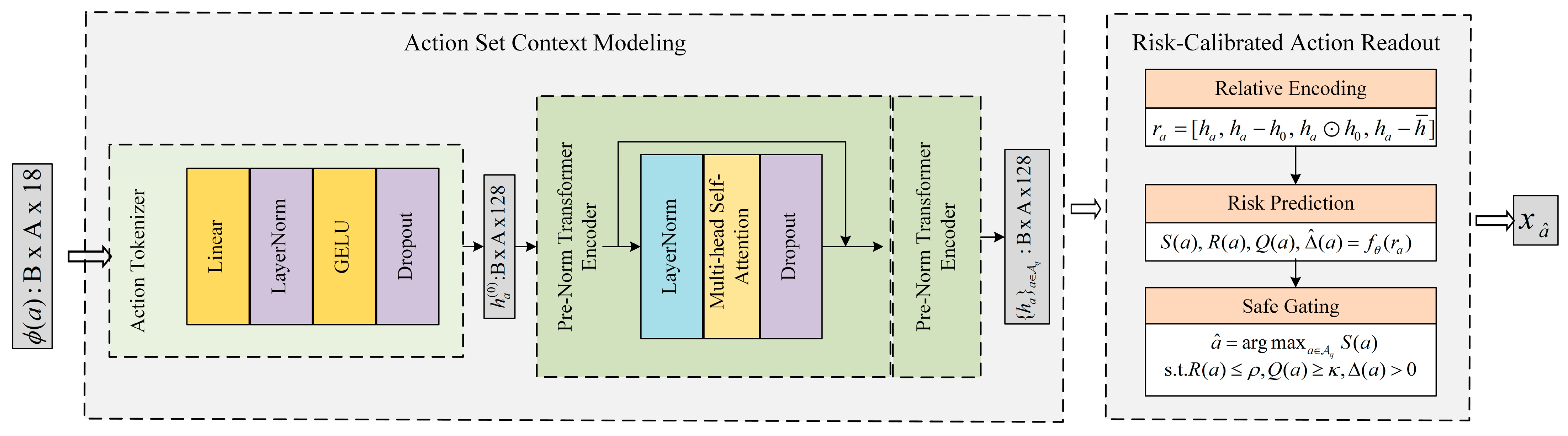
RC-MPAV then performs set-level verification over ${\mathcal{A}}_q$. Each action $a$ is represented by a coordinate $x(a)$ and an inference feature $\varphi (a)$. The feature $\varphi (a)$ is constructed only from the probability field shape, action type, posterior support, and relative positional relationships. It does not contain the true localization error or any information derived from the ground truth. As shown in Figure 4, action features are first encoded as tokens. A Transformer then models dependencies within the same sample and produces context-aware action representations:

$$\left\{\begin{array}{l}{h}_a^{(0)}={\mathrm{MLP}}_{tok}(\varphi (a))\\ {\left\{h_a\right\}}_{a\in {\mathcal{A}}_q}=\mathrm{Transformer}({\left\{h_a^{(0)}\right\}}_{a\in {\mathcal{A}}_q})\end{array}\right.$$

(17)

Let $h_0$ denote the representation of the default action $a_0$, and let $\overline{h}={\displaystyle \frac{1}{\left|{\mathcal{A}}_q\right|}}{\displaystyle \sum _{b\in {\mathcal{A}}_q}{h}_b}$ be the mean contextual representation of the action set. The relative decision feature for action $a$ is constructed as:

$$r_a=[h_a,\hspace{0.33em}{h}_a-h_0,\hspace{0.33em}{h}_a\odot h_0,\hspace{0.33em}{h}_a-\overline{h}]$$

(18)

where $\odot$ denotes element-wise multiplication. RC-MPAV uses $r_a$ to jointly predict the action selection score, integrated switching risk, posterior support mass, and expected error improvement relative to the default action:

$$S(a),\hspace{0.33em}R(a),\hspace{0.33em}Q(a),\hspace{0.33em}\widehat{\Delta }(a)=f_{\theta }(r_a)$$

(19)

where $S\left(a\right)$ denotes the relative utility of selecting action $a$ within the current action set. $R(a)$ denotes the integrated risk of switching to this action. $Q(a)$ denotes the posterior support mass associated with this action. $\widehat{\Delta }(a)$ denotes the expected error improvement relative to the default action.

During inference, RC-MPAV adopts a conservative risk-calibrated decision rule. The default action $a_0$ is retained unless at least one alternative action satisfies the risk, support, and improvement gates. The admissible alternative-action set is defined as:

$${\mathcal{A}}_{safe}=\left\{a\in {\mathcal{A}}_q\backslash \left\{a_0\right\}\mid R(a)\le o,\hspace{0.33em}Q(a)\ge \kappa ,\hspace{0.33em}\widehat{\Delta }(a)>0\right\}$$

(20)

where $o$ is the switching-risk threshold and $\kappa$ is the posterior-support threshold. The final action is selected by:

$$\widehat{a}=\left\{\begin{array}{ll}{a}_0,\hfill & {\mathcal{A}}_{safe}=\varnothing ,\hfill \\ \arg {\max }_{a\in {\mathcal{A}}_{safe}}S(a),\hfill & {\mathcal{A}}_{safe}\ne \varnothing .\hfill \end{array}\right.$$

(21)

The final coordinate is $\widehat{x}=x(\widehat{a})$. This default-retaining rule prevents an alternative posterior peak from overwriting the current estimate unless the alternative has bounded predicted risk, sufficient posterior support, and positive expected improvement. Therefore, RC-MPAV reduces error propagation caused by unsupported or high-risk switching, rather than performing unconstrained peak switching.

To remain consistent with the risk-calibrated decision rule used during inference, RC-MPAV constructs supervision signals by using the default action as the relative reference during training. Let the localization error of action $a$ be $e(a)=\Vert x(a)-x_q{\Vert }_2$, and let the default-action error be $e_0=e(a_0)$. The relative error improvement is defined as $\Delta (a)=e_0-e(a)$.

A positive value of $\Delta (a)$ indicates that action $a$ improves over the default action, whereas a negative value indicates that switching to this action would increase localization error. Based on $\Delta (a)$, the training process provides supervision signals for the optimal action, improvable actions, risky actions, and default-action failure. The training loss of RC-MPAV is defined as:

$${\mathcal{L}}_{RC}={\mathcal{L}}_{choice}+{\lambda }_r{\mathcal{L}}_{risk}+{\lambda }_{\Delta }{\mathcal{L}}_{\Delta }+{\lambda }_{guard}{\mathcal{L}}_{guard}$$

(22)

where ${\mathcal{L}}_{choice}$ supervises the model to identify the readout with the smallest relative error within the action set. ${\mathcal{L}}_{risk}$ calibrates risk judgments for improvement, harm, catastrophic switching, and default-action failure. ${\mathcal{L}}_{\Delta }$ regresses the error change relative to the default action. ${\mathcal{L}}_{guard}$ suppresses excessive switching when the default action is already reliable.

4. Experiments

4.1. Dataset and Experimental Settings

(1)

Dataset

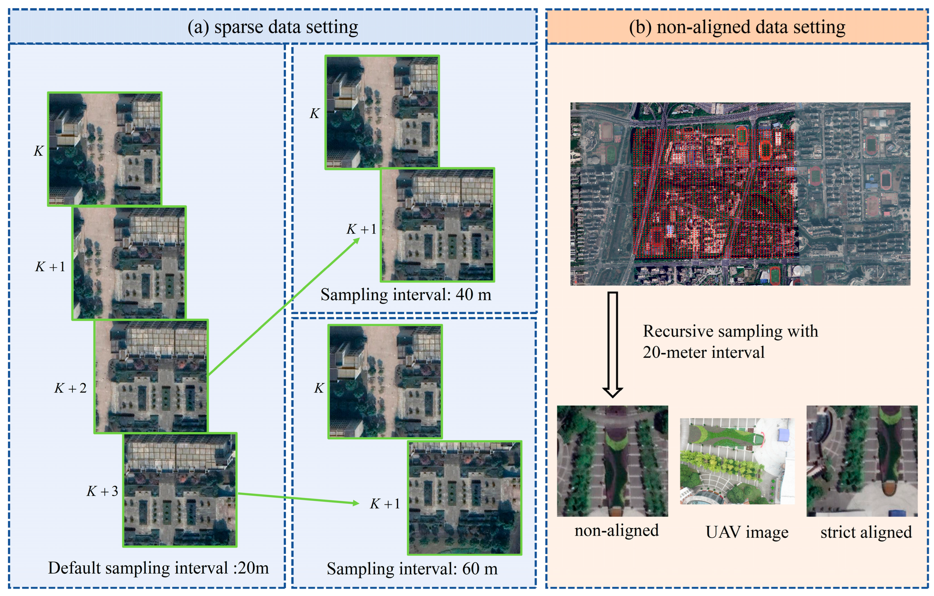
We conduct the main experiments on the DenseUAV dataset. DenseUAV provides UAV query images and their corresponding satellite reference images. It is suitable for evaluating the cross-view self-localization capability of low-altitude UAVs in urban areas. It should be noted that the original satellite gallery of DenseUAV contains multiple satellite tiles at the same geographic coordinate. This setting is essentially a redundant gallery design. To make coordinate localization evaluation clearer, we retain only one satellite tile at each location and construct a default gallery containing 3048 candidate satellite tiles. The satellite sampling interval of this default gallery is approximately 20 m. It is used to evaluate retrieval and coordinate localization performance under the standard DenseUAV setting.

As shown in Figure 5a, we further evaluate the robustness of the method under sparse satellite galleries. In this experiment, the UAV query images remain unchanged, and only the sampling density of the satellite candidate gallery is modified. Specifically, the default gallery has a satellite sampling interval of 20 m. We further perform interval sampling according to the center coordinates of satellite tiles and construct sparse galleries with sampling intervals of 40 m and 60 m. This setting represents practical deployment scenarios where the satellite gallery cannot be arbitrarily densified. It also tests whether discrete top-1 tile-center readout produces more obvious coordinate quantization errors when the gallery becomes sparse. As shown in the figure, the distance between the true UAV location and the nearest available satellite tile center may increase as the satellite sampling interval increases. This experiment, therefore, directly corresponds to the core motivation of this study, namely that discrete gallery anchors limit continuous coordinate localization.

As shown in Figure 5b, we construct a non-aligned satellite gallery to further examine whether the method depends on a strict one-to-one correspondence between the UAV query and the satellite tile center. This experiment reuses the UAV query images and their ground-truth coordinates from DenseUAV but retiles the satellite base map with the same tile resolution and a sampling interval of 20 m as the default gallery. This produces a new gallery containing 2740 candidate satellite tiles. In this non-aligned gallery, the average distance between the UAV ground-truth locations and their nearest satellite tile centers is 12.7 m. Compared with the default gallery, this setting no longer guarantees that the UAV ground-truth coordinate lies near the center of a satellite tile, while keeping the tiling resolution and sampling interval consistent with the aligned setting. It is, therefore, closer to the way satellite tiles are generated from a fixed grid in real map systems. As shown in the figure, the non-aligned satellite gallery breaks the simplified assumption that the query location is equal to the center of a tile. It can, therefore, more directly test the necessity of organizing discrete candidate evidence as a continuous geographic posterior in PFIRNet.

(2)

Evaluation Metrics

We first use retrieval metrics to evaluate whether the model can return the correct or approximately correct candidate region from the satellite gallery. Following the common evaluation protocol in cross-view geo-localization, we use top-K retrieval accuracy, namely Recall@K (R@K), to evaluate whether the correct match appears in the top-K retrieval results. Let the test set contain $N$ query samples, and let ${\mathrm{Rank}}_i$ denote the rank of the correct match for the $i$-th query in the ranked list. R@K is defined as:

$$\mathrm{R}@\mathrm{K}={\displaystyle \frac{1}{N}}{\displaystyle \sum _{i=1}^N\mathbb{I}}({\mathrm{Rank}}_i\le K)$$

(23)

where $\mathbb{I}(\cdot )$ is the indicator function. When the correct match appears within the top-K results, the query is counted as a successful retrieval. We mainly report R@1 to evaluate candidate-region recall when only one relocalization attempt is allowed.

In addition to R@K, we also compute Average Precision (AP) to evaluate retrieval stability over the full ranked list. AP can be regarded as the discrete area under the precision–recall curve and is computed as:

$$\mathrm{AP}={\displaystyle \sum _{k}P}(k)\Delta r(k)$$

(24)

where $k$ denotes the position index in the ranked list, $P(k)$ denotes the precision of the top-$k$ retrieval results, and $\Delta r(k)$ denotes the recall increment from position $k-1$ to position $k$. Compared with R@1, AP does not focus only on the top-ranked candidate. It also reflects the overall distribution of valid candidates in the ranked list.

PFIRNet does not aim only to improve retrieval ranking. Its goal is to convert retrieval evidence into a coordinate-level continuous posterior. Therefore, we do not use a single R@1 value as the main basis for drawing conclusions. Coordinate localization performance is mainly described by median localization error and threshold success rate S@τ. The median localization error is the median of localization errors over all test samples. S@τ denotes the proportion of samples whose localization error does not exceed the threshold τ. In the DenseUAV experiments, we report mean error, median error, S@10m, S@30m, and S@τ 50m to characterize both fine-grained localization accuracy and region-level localization stability under more relaxed thresholds. In the non-aligned satellite gallery, retrieval metrics use the satellite tile nearest to the true UAV coordinate as the proxy positive. However, all coordinate localization metrics are always computed using the true UAV coordinate, rather than the tile center of the proxy positive.

(3)

Hardware and Training Settings

All models are implemented in PyTorch and trained on an NVIDIA GeForce RTX 4090 GPU. The retrieval backbone is the DenseUAV Transformer-based two-branch feature extractor initialized from the released DenseUAV checkpoint, with an input resolution of $224\times 224$ and a 512-dimensional output feature. The DenseUAV training split contains 2256 query IDs, and the independent test split contains $N=777$ queries. To prevent the second stage from directly memorizing first-stage outputs on the same samples, we divide the training IDs according to sample IDs. Specifically, 80% of the training IDs, corresponding to 1805 IDs, are used to train the stage-one CPFL model. After stage-one training is completed, its backbone parameters are frozen. We then run stage-one inference on the remaining 451 training IDs to generate candidate posteriors, default outputs, alternative posterior peaks, action features, and error labels for training the stage-two RC-MPAV module.

For stage one, the annealed geographic scale is defined as:

$${\sigma }_e(t)=\max ({\sigma }_{\min },{\sigma }_0{\gamma }^t)$$

(25)

where ${\sigma }_0=60.0\hspace{0.17em}\mathrm{m}$, ${\sigma }_{\min }=10.0\hspace{0.17em}\mathrm{m}$, and $\gamma =0.92$. When the dataset-adaptive lower-bound option is enabled, the lower bound is additionally constrained by a 5.0 m floor and the 75th percentile of the measured alignment scale. The positive and negative geographic radii are set to $r_p=10.0 \mathrm{m}$ and $r_n=50.0 \mathrm{m}$, respectively. The geographic ranking margin parameter is $\alpha =3.0$, and the candidate similarity temperature is $\tau =0.07$.

The CPFL probability field is constructed on a $192\times 192$ local metric grid with a 30.0 m boundary margin. The coordinate supervision scale is ${\sigma }_g=100.0 \mathrm{m}$. In the reported manuscript experiments, the candidate support spread is set to ${\sigma }_k=30.0 \mathrm{m}$, and the corresponding sensitivity experiment in Section 4.2 evaluates this parameter around the selected operating range. The stage-one candidate-field and ranking terms use ${\lambda }_f=1.0$, ${\lambda }_g=1.0$, and ${\lambda }_t=0.5$. The additional sharp-triplet term uses unit weight. In Equation (12), ${\lambda }_g$ denotes only the geographic classification term.

For stage two, posterior peaks are retained when their response is at least $\rho =0.5$ of the dominant peak and are separated by a minimum distance of 40.0 m before local action generation. The implementation extracts, at most, five posterior basins, uses a 25.0 m NMS radius for basin-level peak suppression, and generates, at most, two ellipse-based actions per basin with ellipse scale 1.0. The local readout radius $r_j$ is estimated adaptively as the radius containing 50% of the posterior mass around the $j$-th basin; when this estimate is unavailable, $r_j$ falls back to 25.0 m. Thus, $r_j$ is not an undisclosed fixed scalar. It is an inference-time radius determined by the local posterior shape.

RC-MPAV uses $\kappa =0.5$ as the minimum posterior-support threshold in the risk-calibrated decision rule. The loss weights in Equation (18) are ${\lambda }_r=1.0$, ${\lambda }_{\Delta }=0.25$, and ${\lambda }_{\mathrm{guard}}=0.75$, while the action-choice term has unit weight. For the internal risk labels, the improvement margin and harm margin are both 5.0 m, the catastrophic-error margin is 100.0 m, and the default-action failure threshold is 25.0 m. The operational fail-safe gates are fixed to a minimum default-failure probability of 0.50, a minimum improvement probability of 0.55, a maximum harm probability of 0.45, a maximum catastrophic probability of 0.10, a minimum support probability of 0.50, and a minimum expected utility gain of 5.0 m. During inference, the default readout is retained unless an alternative action satisfies the risk, support, and positive-gain constraints.

Stage-one training uses AdamW with a learning rate of $1\times {10}^{-5}$, batch size 2, and 40 epochs. Stage-two training freezes the backbone and optimizes the RC-MPAV refinement head with AdamW, a learning rate of $1\times {10}^{-4}$, batch size 8, and 30 epochs. Both stages use a weight decay of $1\times {10}^{-4}$. Mixed-precision training is enabled on the RTX 4090. All final results are evaluated on the independent test set with $N=777$ under the same gallery protocol and coordinate-error calculation procedure.

4.2. Ablation Experiments

(1)

Ablation Study on the Overall Framework

To evaluate the necessity of each core module and their synergy in PFIRNet, we further conduct an overall ablation study on the full pipeline. The results are reported in

Table 2. Ablation study on the overall framework.

AGDS	CPFL	RC-MPAV	R@1↑	AP↑	Med.err.(m)↓	S@10m↑
-	-	-	80.36	69.21	20.12	38.92
√	-	-	83.78	76.27	16.87	44.18
√	√	-	83.78	76.27	14.28	46.44
√	√	√	83.78	76.27	9.84	51.87

. We compare the DenseUAV baseline, the model enhanced with AGDS, the model further equipped with CPFL, and the complete PFIRNet with RC-MPAV. This setting allows us to isolate how distance-aware supervision, continuous probability field readout, and risk-calibrated verification contribute to the final localization performance.

Table 2 shows a steady improvement as the modules are added. AGDS raises R@1 from 80.36% to 83.78% and AP from 69.21% to 76.27%. The median error also drops from 20.12 m to 16.87 m. These changes show that distance-aware geographic supervision improves the retrieval response and makes the candidate ranking more useful for coordinate estimation.

Adding CPFL keeps R@1 and AP unchanged but further reduces the median error to 14.28 m and increases S@10m to 46.44%. This result matches the role of CPFL. It does not aim to retrieve a different candidate list. Instead, it converts the top-k candidates into a continuous coordinate-space posterior, which reduces the dependence on direct tile-center readout.

The complete PFIRNet reduces the median error to 9.84 m and improves S@10m to 51.87%. Since the retrieval metrics remain fixed, this gain mainly comes from the final coordinate decision. RC-MPAV complements CPFL by checking competing posterior peaks and updating the estimate only when an alternative readout is reliable. The ablation, therefore, confirms that the three modules serve different purposes in the same pipeline. AGDS shapes the retrieval response, CPFL builds the continuous coordinate posterior, and RC-MPAV improves the reliability of the final readout.

(2)

Ablation Study on Geographic Distribution Supervision

In UAV-to-satellite localization, nearby satellite tiles often share road structures, building boundaries, or land-cover textures with the query image. If all these candidates are treated as hard negative samples during training, the learned similarity distribution may favor image-identity discrimination rather than faithfully reflecting true geographic distance. To evaluate the effect of Geographic Distribution Supervision, we modify the supervision strategy on the DenseUAV baseline while keeping the basic retrieval framework unchanged. The results are reported in

Table 3. Ablation study on Geographic Distribution Supervision.

Variant	R@1↑	AP↑	Spearman↑	S@10m↑
hard triplet	80.36	69.21	0.36	38.92
Gaussian soft label	78.12	77.24	0.53	35.62
AGDS w/o annealing	81.23	74.73	0.42	33.27
AGDS	83.78	76.27	0.56	44.18

. We compare hard triplet supervision, Gaussian soft labels, AGDS without annealing, and the full AGDS. The metrics evaluate retrieval accuracy, ranking stability, similarity distance consistency, and near-range localization performance.

Table 3 shows that changing the supervision strategy clearly affects both retrieval behavior and coordinate-level localization. The hard triplet baseline achieves 80.36% R@1 and 38.92% S@10m, but its Spearman correlation is only 0.36. This indicates that hard positive–negative supervision can support candidate discrimination, but it does not fully preserve the geographic ordering among nearby satellite tiles.

Gaussian soft labels increase AP to 77.24% and improve Spearman correlation to 0.53. The smoother target distribution, therefore, improves ranking stability and distance consistency. However, R@1 decreases to 78.12%, and S@10m drops to 35.62%. A fixed soft distribution can make the ranked list smoother, but it does not necessarily improve fine-grained localization around the true coordinate.

The comparison between AGDS without annealing and full AGDS further shows the role of adaptive supervision. Without annealing, AGDS improves R@1 to 81.23%, but S@10m decreases to 33.27%. The full AGDS achieves the best R@1, Spearman correlation, and S@10m, reaching 83.78%, 0.56, and 44.18%, respectively. Its AP is slightly lower than that of Gaussian soft labels, but its stronger near-range localization result is more consistent with the objective of UAV self-localization. These results show that distance-aware supervision is most effective when its geographic support is adjusted progressively during training.

(3)

Ablation Study on CPFL

To examine the effect of CPFL, we build on the AGDS setting and compare three coordinate readout strategies. The results are reported in

Table 4. Ablation study on CPFL readout strategies.

Readout	Mean err.(m)↓	Med.err.(m)↓	S@10m↑	S@30m↑	S@50m↑
Top-1 tile center	360.58	16.87	44.18	70.84	75.72
Weighted top-k coordinate	372.07	17.53	39.22	70.63	77.83
CPFL	348.65	14.28	46.44	71.93	76.64

. Top-1 tile center uses the center of the highest-scoring tile directly, weighted top-k coordinate averages multiple candidate coordinates, and CPFL constructs a continuous probability field before readout. These strategies correspond to discrete anchor readout, direct multi-candidate fusion, and spatial posterior modeling.

Table 4 shows that CPFL gives the lowest mean and median localization errors among the three readout strategies. Compared with Top-1 tile center, CPFL reduces the mean error from 360.58 m to 348.65 m and the median error from 16.87 m to 14.28 m. It also improves S@30m from 70.84% to 71.93%. These changes show that direct tile-center readout remains a strong baseline, but it is still limited by the discrete sampling of the satellite gallery.

Weighted top-k coordinate performs worse than Top-1 tile center on mean error, median error, and S@10m. The result suggests that a simple average of high-scoring candidates does not reliably preserve spatial meaning when the candidates are separated in geographic space. CPFL avoids this failure mode by retaining the spatial structure of the candidate responses in a continuous field, rather than collapsing them into one averaged coordinate.

The threshold results are less uniform. The weighted top-k coordinate is slightly higher at S@50m. CPFL, therefore, should not be described as uniformly superior under every threshold. Its main advantage lies in reducing coordinate error and providing a structured posterior for the later risk verification stage.

(4)

Ablation study on RC-MPAV

RC-MPAV is designed to refine the final coordinate readout over the multimodal posterior field produced by CPFL. Although the stage-one probability field already encodes multiple spatial hypotheses, the final estimate may still be affected by unsafe switching among competing peaks. To analyze the contribution of each loss term in RC-MPAV, we compare the complete model with variants obtained by removing one supervision term at a time. In all variants, the same stage-one CPFL readout is used as the starting point, so the comparison isolates the effect of the RC-MPAV training objective itself. The evaluation metrics include median error, S@10m, S@30m, and S@50m, which characterize the average localization error, the typical localization accuracy, and the near-range and region-level success rates, respectively.

As shown in

Table 5. Ablation study on RC-MPAV loss terms.

Variant	Med.err.(m)↓	S@10m↑	S@30m↑	S@50m↑
w/o ${\mathcal{L}}_{choice}$	12.61	46.92	72.48	77.28
w/o ${\mathcal{L}}_{risk}$	11.64	48.17	73.54	79.47
w/o ${\mathcal{L}}_{\Delta }$	10.92	49.69	75.58	81.76
w/o ${\mathcal{L}}_{guard}$	10.68	50.01	76.14	82.03
RC-MPAV	9.84	51.87	76.93	82.54

, the four ablated variants form a clear staircase. Median error moves from 12.61 m to 11.64 m, then to 10.92 m and 10.68 m, while S@10m rises from 46.92% to 48.17%, 49.69%, and 50.01%. The complete RC-MPAV model reaches 9.84 m and 51.87%. The change is gradual rather than abrupt, which suggests that the supervision terms contribute complementary pieces of guidance rather than a single dominant correction.

The threshold scores show a similar pattern. S@30m improves from 72.48% to 76.14% across the ablated variants, and S@50m moves from 77.28% to 82.03%. The complete model reaches 76.93% and 82.54%. The gain is most visible at the stricter 10 m threshold, where the gap to the full model remains largest. RC-MPAV is, therefore, doing more than preserving region-level recall. It is mainly tightening the final readout around the true coordinate and making the peak choice less fragile under multimodal posterior responses.

(5)

Ablation Study on Key Hyperparameters

This supplementary experiment examines two key hyperparameters in CPFL, the number of top-k candidates used for field construction and the Gaussian support spread. The results are reported in

Table 6. Ablation study on top-k posterior field construction.

Top-k	Med.err.(m)↓	S@10m↑	S@30m↑	S@50m↑
8	15.71	44.94	66.85	75.42
16	14.24	46.12	69.15	76.06
32	14.28	46.44	71.93	76.64
64	18.37	41.24	68.39	74.42

and

Table 7. Sensitivity analysis of support spread.

Support Spread (m)	Med.err.(m)↓	S@10m↑	S@30m↑	S@50m↑
20	15.73	45.27	70.14	74.89
30	14.28	46.44	71.93	76.64
40	15.05	45.62	70.92	75.15

. The first part varies top-k to test how much candidate evidence the probability field needs, and the second part fixes top-k at 32 to check how the spatial spread shapes the posterior field.

With only eight candidates, the posterior field has limited spatial support, and the median error remains at 15.71 m. Expanding top-k to 16 tightens the readout, bringing the median error down to 14.24 m and raising S@10m to 46.12%. The 32-candidate setting keeps the median error at essentially the same level, while improving S@30m to 71.93% and S@50m to 76.64%. That makes it the most balanced choice across the full set of thresholds.

The trend changes when top-k is increased to 64. The median error rises to 18.37 m, and S@10m falls to 41.24%. A larger candidate set is then pulling in more distant but visually similar regions, which spreads the posterior response and weakens coordinate readout. In this setting, more candidates do not mean better support. The field becomes less concentrated, and the benefit from additional evidence is offset by noise from less relevant regions. To check the spatial smoothness of the posterior field, we fix top-k at 32 and vary the Gaussian support spread.

The 30 m setting gives the strongest overall result. A smaller spread sharpens the field, but it also makes the posterior response easier to fragment. A larger spread broadens the support, yet the peaks become less distinct. Both changes weaken the readout compared with the 30 m setting, which keeps enough locality to preserve the main peaks while still providing stable spatial support. Taken together, the two experiments point to the same setting principle. CPFL benefits from a moderate amount of candidate evidence and a moderate Gaussian spread, rather than from an aggressive expansion in either direction.

4.3. Comparison with Cross-View Localization Algorithms

To comprehensively evaluate the localization performance of PFIRNet on DenseUAV, we compare it with one-stage retrieval methods and two-stage matching methods. The one-stage methods include LPN, FSRA, DenseUAV, and DenseUAV + LPN. These methods mainly rely on cross-view feature retrieval and usually use the top-ranked satellite tile as the localization basis. The two-stage methods further introduce local matchers after region retrieval, including LoFTR, ASpanFormer, and RoMa-Tiny, to estimate finer positions within candidate satellite regions. For these two-stage baselines, R@1 and AP are determined by their stage-one retrieval results. The subsequent localization metrics reflect the outputs after local matching or coordinate refinement. In the table, Ours Stage-one corresponds to the stage-one model composed of AGDS and CPFL. Ours further adds RC-MPAV and performs risk-controlled readout over the multimodal posterior in the continuous probability field. All methods are re-evaluated under the same DenseUAV coordinate evaluation protocol to ensure that retrieval metrics and meter-level localization metrics are comparable.

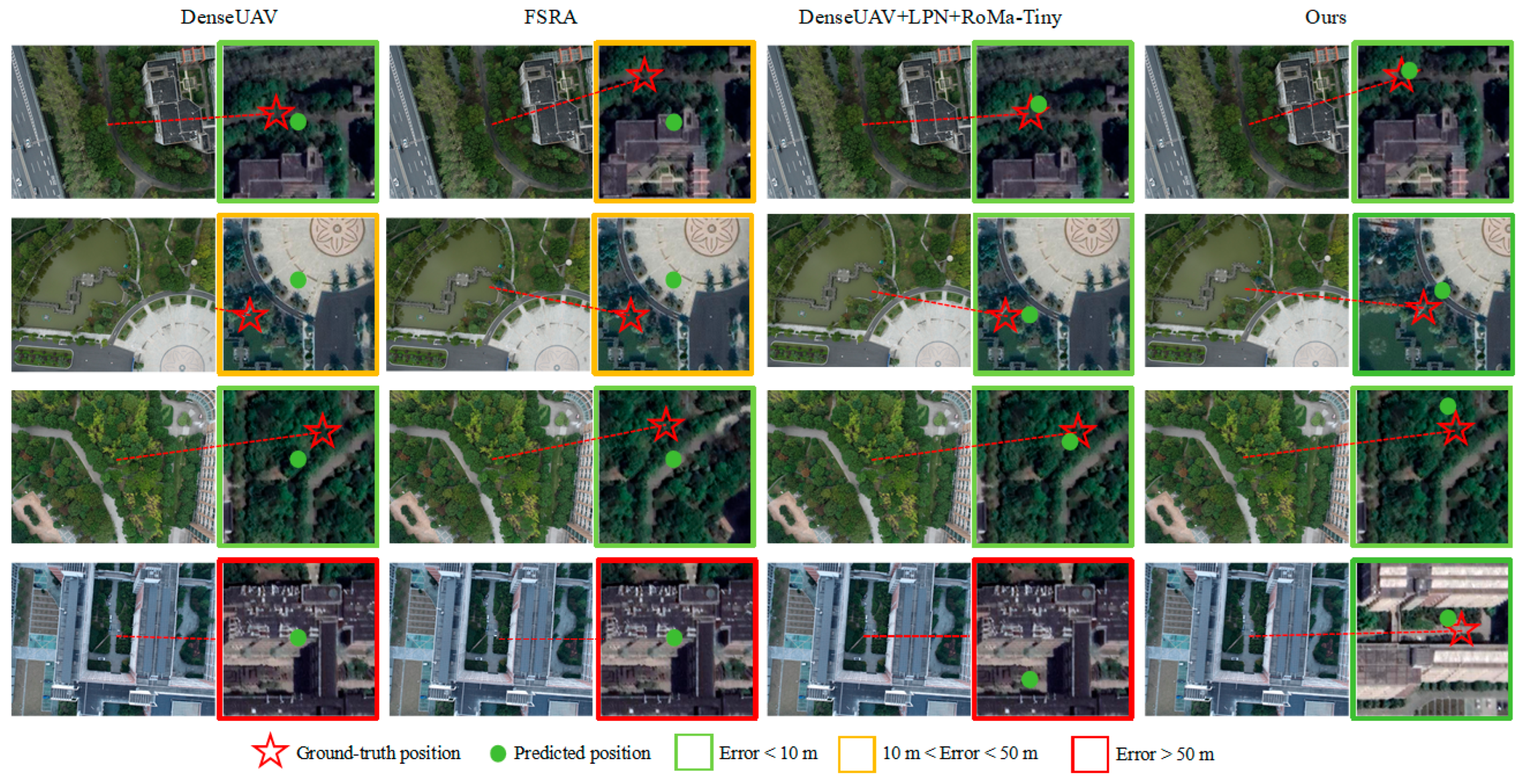
As shown in Figure 6, the output of PFIRNet is not restricted to the center of a single satellite tile. Instead, it provides a localization result in continuous coordinate space. Compared with traditional retrieval methods that directly return discrete candidate centers, PFIRNet uses top-k candidates to construct a probability field and reads out coordinates from the posterior distribution. These coordinates are closer to the true location. In several visualization examples, the predicted points of DenseUAV and FSRA can deviate from the true location. When the top-ranked candidate falls in an incorrect region, the local matching in DenseUAV + LPN + RoMa-Tiny also struggles to establish stable correspondences, and the localization error increases substantially. In contrast, PFIRNet can still use the continuous posterior and the second-stage multi-peak verification to constrain the final prediction to a position closer to the true coordinate.

This visualization also reflects the difference between PFIRNet and traditional two-stage matching pipelines. Local matching methods depend on the reliability of the candidate region from the previous stage. Once the retrieved candidate has deviated from the true region, subsequent matching can usually only refine the estimate within the wrong spatial range. PFIRNet preserves multiple posterior peaks and their spatial support relationships. It then performs constrained selection among the default peak, local posterior readout, and alternative peaks. Therefore, even when some retrieval baselines show obvious offsets, PFIRNet may still recover a more reasonable coordinate from an effective posterior peak in the probability field.

Table 8. Localization results on DenseUAV dataset.

Type	Method	R@1	AP	Mean err.(m)	Med.err.(m)	S@10m	S@30m	S@50m
One-stage	LPN [3]	34.62	24.96	549.53	72.84	10.76	25.63	43.18
	FSRA [46]	81.71	71.95	372.15	18.74	37.42	66.35	72.91
	DenseUAV [5]	80.36	69.21	381.24	20.12	38.92	65.44	70.13
	DenseUAV [5] + LPN [3]	82.86	73.32	367.18	16.36	42.47	68.94	74.16
	Ours Stage-one	83.78	76.27	348.65	14.28	46.44	71.93	76.64
Two-stage	FSRA [46] + LoFTR [37]	81.71	71.95	358.73	16.34	43.60	71.20	76.40
	DenseUAV [5] + LoFTR [37]	80.36	69.21	367.14	18.13	41.34	74.52	79.18
	DenseUAV [5] + ASpanFormer [38]	80.36	69.21	360.85	17.94	43.72	75.54	79.68
	DenseUAV [5] + RoMa-Tiny [40]	80.36	69.21	364.57	17.98	42.87	75.43	80.10
	DenseUAV + LPN [3] + LoFTR [37]	82.86	73.32	342.49	14.34	44.83	75.25	79.80
	DenseUAV + LPN [3] + ASpanFormer [38]	82.86	73.32	334.71	13.26	46.76	75.86	80.21
	DenseUAV + LPN [3] + RoMa-Tiny [40]	82.86	73.32	332.58	13.24	47.24	76.23	80.53
	Ours Stage-one + LoFTR [37]	83.78	76.27	327.63	12.61	48.73	77.36	80.67
	Ours Stage-one + RoMa-Tiny [40]	83.78	76.27	314.91	11.21	49.72	77.61	81.36
	Ours	83.78	76.27	287.23	9.84	51.87	76.93	82.54

compares PFIRNet with both one-stage retrieval methods and two-stage matching methods on DenseUAV. Among the one-stage methods, Ours Stage-one achieves the best retrieval performance, with R@1 of 83.78% and AP of 76.27%. It also reaches 46.44% at S@10m, 71.93% at S@30m, and 76.64% at S@50m. These results place it ahead of the other one-stage baselines on both candidate recall and threshold-based localization accuracy.

The median error of Ours Stage-one remains 14.28 m, which is better than DenseUAV and the DenseUAV + LPN variant but still leaves room for refinement at the final readout stage. The gap between retrieval strength and coordinate precision is visible here. A strong ranked list does not fully remove long-tail errors or ambiguity among nearby posterior peaks.

DenseUAV + LPN + RoMa-Tiny is the strongest traditional two-stage baseline. It reaches a median error of 13.24 m, with S@10m, S@30m, and S@50m of 47.24%, 76.23%, and 80.53%, respectively. PFIRNet improves on this result across all major metrics. The full model reduces the median error to 9.84 m and raises S@10m, S@30m, and S@50m to 51.87%, 76.93%, and 82.54%. Compared with DenseUAV + LPN + RoMa-Tiny, the median error drops by 3.40 m, while the threshold success rates increase by 4.63, 0.70, and 2.01 percentage points.

The comparison suggests that PFIRNet is not gaining performance only from better retrieval ranking. Traditional two-stage pipelines still depend on local matching inside the retrieved region. PFIRNet instead turns the top-k retrieval evidence into a continuous probability field and uses RC-MPAV to make the final coordinate decision more stable. That combination improves both typical localization error and threshold success rates, especially at the stricter 10 m level.

These results show that the advantage of PFIRNet does not come only from a higher retrieval ranking. Traditional two-stage methods rely on local matchers to refine the estimate within the retrieved candidate region. In contrast, PFIRNet organizes top-k retrieval evidence into a continuous probability field and uses RC-MPAV to perform risk-controlled selection over multiple posterior peaks. As a result, PFIRNet achieves higher retrieval stability, lower typical localization error, and higher threshold success rates. This shows that coordinate-level posterior inference is better suited to this task than simple discrete candidate selection or post-retrieval local matching.

4.4. Motivation Validation Experiments

(1)

Validation on Sparse Satellite Galleries

To evaluate the dependence of the method on satellite gallery density, we gradually increase the satellite sampling interval while keeping the DenseUAV query set unchanged. We compare localization performance under three settings: default, 40 m, and 60 m. This experiment corresponds to a common constraint in real deployment. The satellite gallery cannot be densified without limit, and the offset between discrete tile centers and true UAV coordinates becomes more pronounced as the sampling interval increases.

As shown in

Table 9. DenseUAV localization results under different satellite sampling intervals.

Sampling Interval	Method	AP↑	Mean err.(m)↓	Med.err.(m)↓	S@10m↑	S@30m↑	S@50m↑
default	DenseUAV	69.21	381.24	20.12	38.92	65.44	70.13
	Ours	76.27	287.23	9.84	51.87	76.93	82.54
40 m	DenseUAV	46.19	401.62	28.13	30.43	55.27	64.61
	Ours	62.13	337.94	14.03	38.16	64.35	79.63
60 m	DenseUAV	33.26	469.42	46.13	13.74	30.26	47.92
	Ours	57.13	371.94	18.64	27.16	43.48	67.29

, the DenseUAV baseline degrades substantially as the satellite sampling interval increases. Under the default setting, DenseUAV achieves 69.21% AP, 20.12 m median localization error, and S@10m, S@30m, and S@50m values of 38.92%, 65.44%, and 70.13%. When the sampling interval increases to 40 m, AP decreases to 46.19%, the median error increases to 28.13 m, and S@10m decreases to 30.43%. Under the 60 m setting, AP further drops to 33.26%, the median error rises to 46.13 m, and S@10m is reduced to 13.74%. The trend shows that sparse satellite galleries weaken both retrieval stability and fine-grained coordinate accuracy for discrete retrieval-based localization.

Ours outperforms DenseUAV under all sampling intervals, and the advantage becomes more evident in the sparse settings. Under the default setting, AP increases from 69.21% to 76.27%, and the median error decreases from 20.12 m to 9.84 m. At a 40 m sampling interval, Ours reaches 62.13% AP and 14.03 m median error, improving AP by 15.94 percentage points and reducing the median error by 14.10 m. S@50m also rises from 64.61% to 79.63%. At the 60 m interval, Ours retains 57.13% AP and 18.64 m median error, compared with 33.26% AP and 46.13 m for DenseUAV. The corresponding improvements are 23.87 percentage points in AP and 27.49 m in median error. These results indicate that PFIRNet is more robust when the satellite gallery becomes sparse. It mitigates the localization error caused by increasing tile-center spacing through continuous posterior inference.

(2)

Localization Robustness under Non-Aligned Satellite Galleries

To examine whether the model depends on a strict correspondence between the UAV query location and the satellite tile center, we further construct a non-aligned satellite gallery. Compared with the strictly aligned setting, the non-aligned setting reorganizes satellite tiling so that the true UAV coordinate no longer falls near a candidate tile center by default. This setting is closer to practical map tiling scenarios. It also directly tests whether the model can use off-center satellite tiles as evidence in continuous space.

As shown in

Table 10. DenseUAV localization results under strictly aligned and non-aligned satellite galleries.

Gallery Setting	Method	AP↑	Mean err.(m)↓	Med.err.(m)↓	S@10m↑	S@30m↑	S@50m↑
strict aligned	DenseUAV	69.21	381.24	20.12	38.92	65.44	70.13
	Ours	76.27	287.23	9.84	51.87	76.93	82.54
non-aligned	DenseUAV	62.41	424.74	32.63	14.37	45.44	64.13
	Ours	75.73	317.02	12.31	46.87	72.17	81.74

, non-aligned satellite galleries substantially weaken the coordinate localization ability of the DenseUAV baseline. Its AP decreases from 69.21% to 62.41%, and its median localization error increases from 20.12 m to 32.63 m. The change is more visible at S@10m, which drops from 38.92% to 14.37%. This shows that traditional discrete retrieval readout is strongly affected when satellite tile centers are no longer strictly aligned with true UAV locations. It is especially difficult for this readout to maintain fine-grained localization accuracy within the 10 m threshold.

Ours remains much more stable under the non-aligned setting. AP changes only slightly, from 76.27% to 75.73%, while the median localization error increases from 9.84 m to 12.31 m. At the same time, S@10m remains at 46.87%, and S@30m and S@50m reach 72.17% and 81.74%, respectively. Compared with DenseUAV under the non-aligned setting, Ours reduces the median localization error by 20.32 m and improves S@10m, S@30m, and S@50m by 32.50, 26.73, and 17.61 percentage points. These results show that PFIRNet does not rely on the single-positive assumption of strict center alignment. Instead, it maintains more reliable coordinate localization in non-aligned satellite galleries through distance-aware supervision and continuous probability field readout.

5. Discussion

5.1. Complexity Analysis

The additional computation of PFIRNet mainly occurs on the post-retrieval top-k candidate set, rather than on the full satellite gallery. If traditional retrieval-based methods aim to improve coordinate accuracy by using a denser satellite gallery, they usually increase the gallery size, feature storage, and online similarity computation cost at the same time. Post-retrieval matching methods need to perform local or dense matching between retrieved candidates and the UAV image. Their inference cost increases with the number of candidate attempts. In contrast, PFIRNet first reuses the top-k candidates produced by the retrieval network. It then lifts candidate similarities and coordinates into a continuous probability field and performs risk-calibrated verification only on the action set generated from a small number of posterior peaks. As shown in

Table 11. Complexity analysis of different methods.

Variant	Params↓	Time↓	Med.err.(m)↓	S@10m↑
DenseUAV	24.03 M	0.17 s	20.12	38.92
Ours Stage-one	24.03 M	0.17 s	14.28	46.44
DenseUAV + LoFTR	35.59 M	0.38 s	18.13	41.34
DenseUAV + RoMa-Tiny	30.82 M	0.45 s	17.98	42.87
Ours	25.29 M	0.26 s	9.84	51.87

, Ours Stage-one achieves better localization accuracy with a parameter count and inference time close to those of DenseUAV. In addition, Ours uses fewer parameters and has a shorter inference time than post-retrieval matching schemes that introduce LoFTR or RoMa-Tiny. This indicates that the method provides a favorable balance between accuracy improvement and deployment efficiency.

5.2. Long-Tail Error Analysis

PFIRNet reduces long-tail localization error by turning top-k retrieval evidence into a continuous coordinate posterior and using risk-calibrated verification to avoid unsafe peak switching. As shown in

Table 12. Long-tail error analysis of localization results.

Method	Mean err.(m)↓	Med.err.(m)↓	P75 (m)↓	P90 (m)↓	P95 (m)↓
DenseUAV	381.24	20.12	24.13	1447.83	3254.46
Ours Stage-one	348.65	14.28	17.84	1258.41	3132.74
Ours	287.23	9.84	14.14	782.54	2569.18

, DenseUAV still has a mean error of 381.24 m and a P95 of 3254.46 m. Ours Stage-one already lowers both the median and the upper tail, and the full model reduces them further to 9.84 m and 2569.18 m. The change is not just a shift in the typical case. It also compresses the rare large failures that dominate the average error. Even so, the tail is not removed completely. The remaining gap between the median and the upper-percentile errors suggests that a few difficult cases are still unresolved, most likely when candidate support is weak or the posterior peaks are too close to separate cleanly. PFIRNet reduces those failures, but it does not eliminate them.

5.3. Limitation Analysis

Although PFIRNet mitigates the localization error caused by discrete tile centers through continuous probability fields and risk-calibrated readout, it still has several limitations. First, the experiments mainly focus on DenseUAV and its extended gallery protocols. These settings evaluate robustness to changes in gallery sampling density and non-strict tile-center alignment, but they do not fully cover appearance variations across cities, seasons, sensors, and more complex low-altitude flight scenarios. Second, PFIRNet still relies on the stage-one top-k candidates to provide valid spatial support for the probability field. If candidates near the true location are completely missed during retrieval, the corrective ability of subsequent probability field construction and multi-peak action verification will also be limited. Third, the current evaluation is based on a fixed test protocol and does not include repeated training runs or paired per-query statistical testing. The reported comparisons, therefore, characterize empirical performance under the shared benchmark setting but do not establish formal statistical significance or quantify run-to-run variability. Future work will extend the evaluation to multi-city, multi-temporal, and cross-sensor data, while also incorporating repeated-run statistical analysis. It will further explore dynamic candidate expansion, trajectory priors, and continuous position encoding mechanisms to improve stability and adaptability under more complex deployment conditions.

6. Conclusions

We proposed PFIRNet, a continuous Probability Field Inference Network. The framework first uses Adaptive Geographic Distribution Supervision to introduce metric distance relationships into candidate response learning. This allows retrieval results to reflect not only visual similarity but also geographic proximity structure. It then uses Continuous Probability Field Localization to lift top-k candidates and their coordinates into a coordinate-space posterior distribution. This design removes the discrete constraint of single tile-center readout. Finally, Risk-Calibrated Multi-Peak Action Verification performs constrained selection among multiple posterior peaks. It suppresses unreliable switching and improves the stability of the final coordinate readout. Experiments on DenseUAV and its sparse and non-aligned satellite galleries show that PFIRNet substantially reduces typical localization error while maintaining a small model size and low inference cost. PFIRNet also maintains more stable localization performance when the satellite gallery becomes sparse or when the tile-center correspondence is disrupted. These results indicate that organizing cross-view retrieval evidence as a continuous geographic posterior is an effective way to improve the accuracy and deployment adaptability of GNSS-degraded low-altitude remote-sensing self-localization.

References

1. Workman, S.; Souvenir, R.; Jacobs, N. Wide-Area Image Geolocalization with Aerial Reference Imagery. In Proceedings of the 2015 IEEE International Conference on Computer Vision (ICCV), Santiago, Chile, 7–13 December 2015; pp. 3961–3969. [Google Scholar] [CrossRef] [Scilit]
2. Zheng, Z.; Wei, Y.; Yang, Y. University-1652: A Multi-View Multi-Source Benchmark for Drone-Based Geo-Localization. In Proceedings of the 28th ACM International Conference on Multimedia, Seattle, WA, USA, 12–16 October 2020; pp. 1395–1403. [Google Scholar] [CrossRef] [Scilit]
3. Wang, T.; Zheng, Z.; Yan, C.; Zhang, J.; Sun, Y.; Zheng, B.; Yang, Y. Each Part Matters: Local Patterns Facilitate Cross-View Geo-Localization. IEEE Trans. Circuits Syst. Video Technol. 2022, 32, 867–879. [Google Scholar] [CrossRef] [Scilit]
4. Zhu, S.; Shah, M.; Chen, C. TransGeo: Transformer Is All You Need for Cross-View Image Geo-Localization. In Proceedings of the 2022 IEEE/CVF Conference on Computer Vision and Pattern Recognition (CVPR), New Orleans, LA, USA, 18–24 June 2022; pp. 1152–1161. [Google Scholar] [CrossRef] [Scilit]
5. Dai, M.; Zheng, E.; Feng, Z.; Qi, L.; Zhuang, J.; Yang, W. Vision-Based UAV Self-Positioning in Low-Altitude Urban Environments. IEEE Trans. Image Process. 2024, 33, 493–508. [Google Scholar] [CrossRef] [Scilit] [PubMed]
6. Li, M.; Wang, Z.; Huo, G.; Chen, W.; Zhao, X. A Deep Learning Framework with Geographic Information Adaptive Loss for Remote Sensing Images Based UAV Self-Positioning. In IAF Symposium on Integrated Applications; International Astronautical Federation: Paris, France, 2024; pp. 8–19. [Google Scholar] [CrossRef] [Scilit]
7. Ye, Y.; Teng, X.; Chen, S.; Li, Z.; Liu, L.; Yu, Q.; Tan, T. Exploring the Best Way for UAV Visual Localization under Low-Altitude Multi-View Observation Condition: A Benchmark. arXiv 2025, arXiv:2503.10692. [Google Scholar]
8. Deuser, F.; Habel, K.; Oswald, N. Sample4Geo: Hard Negative Sampling for Cross-View Geo-Localisation. In Proceedings of the 2023 IEEE/CVF International Conference on Computer Vision (ICCV), Paris, France, 1–6 October 2023; pp. 16801–16810. [Google Scholar] [CrossRef] [Scilit]
9. Zhu, S.; Yang, T.; Chen, C. VIGOR: Cross-View Image Geo-Localization beyond One-to-One Retrieval. In Proceedings of the 2021 IEEE/CVF Conference on Computer Vision and Pattern Recognition (CVPR), Nashville, TN, USA, 20–25 June 2021; pp. 5316–5325. [Google Scholar] [CrossRef] [Scilit]
10. Wang, X.; Xu, R.; Cui, Z.; Wan, Z.; Zhang, Y. Fine-Grained Cross-View Geo-Localization Using a Correlation-Aware Homography Estimator. In Advances in Neural Information Processing Systems 36; Neural Information Processing Systems Foundation: La Jolla, CA, USA, 2023; pp. 5301–5319. [Google Scholar] [CrossRef] [Scilit]
11. Chen, J.; Zheng, E.; Dai, M.; Chen, Y.; Lu, Y. OS-FPI: A Coarse-to-Fine One-Stream Network for UAV Geolocalization. IEEE J. Sel. Top. Appl. Earth Obs. Remote Sens. 2024, 17, 7852–7866. [Google Scholar] [CrossRef] [Scilit]
12. Tang, B.; Lu, R.; Yang, X.; Li, Y.; Li, Y.; Zhang, D.; Chen, S. R2PLoc: A Region-to-Point UAV Visual Geo-Localization Framework Leveraging Hierarchical Semantic Representation. IEEE Trans. Geosci. Remote Sens. 2025, 63, 1–18. [Google Scholar] [CrossRef] [Scilit]
13. Hu, S.; Feng, M.; Nguyen, R.M.H.; Lee, G.H. CVM-Net: Cross-View Matching Network for Image-Based Ground-to-Aerial Geo-Localization. In Proceedings of the 2018 IEEE/CVF Conference on Computer Vision and Pattern Recognition, Salt Lake City, UT, USA, 18–23 June 2018; pp. 7258–7267. [Google Scholar] [CrossRef] [Scilit]
14. Shi, Y.; Liu, L.; Yu, X.; Li, H. Spatial-Aware Feature Aggregation for Image Based Cross-View Geo-Localization. In Advances in Neural Information Processing Systems 32; Curran Associates: Red Hook, NY, USA, 2019. [Google Scholar]
15. Liu, L.; Li, H. Lending Orientation to Neural Networks for Cross-View Geo-Localization. In Proceedings of the 2019 IEEE/CVF Conference on Computer Vision and Pattern Recognition (CVPR), Long Beach, CA, USA, 15–20 June 2019; pp. 5617–5626. [Google Scholar] [CrossRef] [Scilit]
16. Zhu, R.; Yin, L.; Yang, M.; Wu, F.; Yang, Y.; Hu, W. SUES-200: A Multi-Height Multi-Scene Cross-View Image Benchmark Across Drone and Satellite. IEEE Trans. Circuits Syst. Video Technol. 2023, 33, 4825–4839. [Google Scholar] [CrossRef] [Scilit]
17. Xu, W.; Yao, Y.; Cao, J.; Wei, Z.; Liu, C.; Wang, J.; Peng, M. UAV-VisLoc: A Large-Scale Dataset for UAV Visual Localization. arXiv 2024, arXiv:2405.11936. [Google Scholar]
18. Shen, T.; Wei, Y.; Kang, L.; Wan, S.; Yang, Y.-H. MCCG: A ConvNeXt-Based Multiple-Classifier Method for Cross-View Geo-Localization. IEEE Trans. Circuits Syst. Video Technol. 2024, 34, 1456–1468. [Google Scholar] [CrossRef] [Scilit]
19. Ge, F.; Zhang, Y.; Liu, Y.; Wang, G.; Coleman, S.; Kerr, D.; Wang, L. Multibranch Joint Representation Learning Based on Information Fusion Strategy for Cross-View Geo-Localization. IEEE Trans. Geosci. Remote Sens. 2024, 62, 1–16. [Google Scholar] [CrossRef] [Scilit]
20. Chen, Z.; Yang, Z.-X.; Rong, H.-J. Multilevel Embedding and Alignment Network With Consistency and Invariance Learning for Cross-View Geo-Localization. IEEE Trans. Geosci. Remote Sens. 2025, 63, 5625615. [Google Scholar] [CrossRef] [Scilit]
21. Huang, G.; Zhou, Y.; Zhao, L.; Gan, W. CV-Cities: Advancing Cross-View Geo-Localization in Global Cities. IEEE J. Sel. Top. Appl. Earth Obs. Remote Sens. 2025, 18, 1592–1606. [Google Scholar] [CrossRef] [Scilit]
22. Feng, T.; Li, Q.; Wang, X.; Wang, M.; Li, G.; Zhu, W. Multi-Weather Cross-View Geo-Localization Using Denoising Diffusion Models. In Proceedings of the 2nd Workshop on UAVs in Multimedia: Capturing the World from a New Perspective, Melbourne, VIC, Australia, 28 October–1 November 2024; pp. 35–39. [Google Scholar] [CrossRef] [Scilit]
23. Song, Z.; Zhang, J.; Wang, D.; Zhou, Z.; Liu, W.; Guo, H.; Wang, E.; Du, B. GeoBridge: A Semantic-Anchored Multi-View Foundation Model Bridging Images and Text for Geo-Localization. arXiv 2025, arXiv:2512.02697. [Google Scholar]
24. Pillai, M.S.; Rizve, M.N.; Shah, M. GAReT: Cross-View Video Geolocalization with Adapters and Auto-Regressive Transformers. In Computer Vision—ECCV 2024; Springer Nature Switzerland: Cham, Switzerland, 2024; pp. 466–483. [Google Scholar] [CrossRef] [Scilit]
25. Keetha, N.; Mishra, A.; Karhade, J.; Jatavallabhula, K.M.; Scherer, S.; Krishna, M.; Garg, S. AnyLoc: Towards Universal Visual Place Recognition. IEEE Robot. Autom. Lett. 2024, 9, 1286–1293. [Google Scholar] [CrossRef] [Scilit]
26. Berton, G.; Trivigno, G.; Caputo, B.; Masone, C. EigenPlaces: Training Viewpoint Robust Models for Visual Place Recognition. In Proceedings of the 2023 IEEE/CVF International Conference on Computer Vision (ICCV), Paris, France, 1–6 October 2023; pp. 11046–11056. [Google Scholar] [CrossRef] [Scilit]
27. Mi, L.; Xu, C.; Castillo-Navarro, J.; Montariol, S.; Yang, W.; Bosselut, A.; Tuia, D. ConGeo: Robust Cross-View Geo-Localization Across Ground View Variations. In Computer Vision—ECCV 2024; Springer Nature Switzerland: Cham, Switzerland, 2025; pp. 214–230. [Google Scholar] [CrossRef] [Scilit]
28. Zhang, X.; Li, X.; Sultani, W.; Zhou, Y.; Wshah, S. Cross-View Geo-Localization via Learning Disentangled Geometric Layout Correspondence. Proc. AAAI Conf. Artif. Intell. 2023, 37, 3480–3488. [Google Scholar] [CrossRef] [Scilit]
29. Zhang, X.; Li, X.; Sultani, W.; Chen, C.; Wshah, S. GeoDTR+: Toward Generic Cross-View Geolocalization via Geometric Disentanglement. IEEE Trans. Pattern Anal. Mach. Intell. 2024, 46, 10419–10433. [Google Scholar] [CrossRef] [Scilit] [PubMed]
30. Xia, P.; Wan, Y.; Zheng, Z.; Zhang, Y.; Deng, J. Enhancing Cross-View Geo-Localization With Domain Alignment and Scene Consistency. IEEE Trans. Circuits Syst. Video Technol. 2024, 34, 13271–13281. [Google Scholar] [CrossRef] [Scilit]
31. Chen, G.; Huang, G.; Yuan, X.; Chen, X.; Zhong, G.; Pun, C.-M. Cross-View Geo-Localization via Learning Correspondence Semantic Similarity Knowledge. In MultiMedia Modeling; Springer Nature: Singapore, 2025; pp. 220–233. [Google Scholar] [CrossRef] [Scilit]
32. Li, G.; Qian, M.; Xia, G.-S. Unleashing Unlabeled Data: A Paradigm for Cross-View Geo-Localization. In Proceedings of the 2024 IEEE/CVF Conference on Computer Vision and Pattern Recognition (CVPR), Seattle, WA, USA, 17–21 June 2024; pp. 16719–16729. [Google Scholar] [CrossRef] [Scilit]
33. Wang, X.; Zhang, L.; Fan, Z.; Liu, Y.; Chen, C.; Deng, F. From Coarse to Fine: A Matching and Alignment Framework for Unsupervised Cross-View Geo-Localization. Proc. AAAI Conf. Artif. Intell. 2025, 39, 8024–8032. [Google Scholar] [CrossRef] [Scilit]
34. Cepeda, V.V.; Nayak, G.K.; Shah, M. GeoCLIP: CLIP-Inspired Alignment between Locations and Images for Effective Worldwide Geo-Localization. In Advances in Neural Information Processing Systems 36; Neural Information Processing Systems Foundation: La Jolla, CA, USA, 2023; pp. 8690–8701. [Google Scholar] [CrossRef] [Scilit]
35. Hu, Y.; Zeng, Q. GRiM-Net: A Two-Stage Cross-View Visual Localization Framework for UAVs. Remote Sens. 2026, 18, 1477. [Google Scholar] [CrossRef] [Scilit]
36. Sarlin, P.-E.; DeTone, D.; Malisiewicz, T.; Rabinovich, A. SuperGlue: Learning Feature Matching With Graph Neural Networks. In Proceedings of the 2020 IEEE/CVF Conference on Computer Vision and Pattern Recognition (CVPR), Seattle, WA, USA, 13–19 June 2020; pp. 4937–4946. [Google Scholar] [CrossRef] [Scilit]
37. Sun, J.; Shen, Z.; Wang, Y.; Bao, H.; Zhou, X. LoFTR: Detector-Free Local Feature Matching with Transformers. In Proceedings of the 2021 IEEE/CVF Conference on Computer Vision and Pattern Recognition (CVPR), Nashville, TN, USA, 20–25 June 2021; pp. 8918–8927. [Google Scholar] [CrossRef] [Scilit]
38. Chen, H.; Luo, Z.; Zhou, L.; Tian, Y.; Zhen, M.; Fang, T.; McKinnon, D.; Tsin, Y.; Quan, L. ASpanFormer: Detector-Free Image Matching with Adaptive Span Transformer. In Computer Vision—ECCV 2022; Springer Nature: Cham, Switzerland, 2022; pp. 20–36. [Google Scholar] [CrossRef] [Scilit]
39. Lindenberger, P.; Sarlin, P.-E.; Pollefeys, M. LightGlue: Local Feature Matching at Light Speed. In Proceedings of the 2023 IEEE/CVF International Conference on Computer Vision (ICCV), Paris, France, 1–6 October 2023; pp. 17581–17592. [Google Scholar] [CrossRef] [Scilit]
40. Edstedt, J.; Sun, Q.; Bokman, G.; Wadenback, M.; Felsberg, M. RoMa: Robust Dense Feature Matching. In Proceedings of the 2024 IEEE/CVF Conference on Computer Vision and Pattern Recognition (CVPR), Seattle, WA, USA, 17–21 June 2024; pp. 19790–19800. [Google Scholar] [CrossRef] [Scilit]
41. Li, W.; Weng, D.; Gao, C.; Du, Q. SwinMatcher: Universal Cross-Modal Remote Sensing Image Matching With Interactive Swin Transformer. IEEE Trans. Geosci. Remote Sens. 2025, 63, 4705916. [Google Scholar] [CrossRef] [Scilit]
42. Wang, B.; Wang, S.; Han, Y.; Xu, L.; Ye, D. LiteSAM: Lightweight and Robust Feature Matching for Satellite and Aerial Imagery. Remote Sens. 2025, 17, 3349. [Google Scholar] [CrossRef] [Scilit]
43. Liu, K.; Zhou, H.; Xu, R.; Wang, P.; Song, M.; Zhang, H. Beyond Matching to Tiles: Bridging Unaligned Aerial and Satellite Views for Vision-Only UAV Navigation. arXiv 2026, arXiv:2603.22153. [Google Scholar]
44. Li, H.; Yang, W.; Xu, F.; Tan, H.; Zhang, H.; Li, S.; Xia, G.-S. Unifying UAV Cross-View Geo-Localization via 3D Geometric Perception. arXiv 2026, arXiv:2604.01747. [Google Scholar]
45. Shetty, A.; Gao, G.X. UAV Pose Estimation Using Cross-View Geolocalization with Satellite Imagery. In Proceedings of the 2019 International Conference on Robotics and Automation (ICRA), Montreal, QC, Canada, 20–24 May 2019; pp. 1827–1833. [Google Scholar] [CrossRef] [Scilit]
46. Dai, M.; Hu, J.; Zhuang, J.; Zheng, E. A Transformer-Based Feature Segmentation and Region Alignment Method for UAV-View Geo-Localization. IEEE Trans. Circuits Syst. Video Technol. 2022, 32, 4376–4389. [Google Scholar] [CrossRef] [Scilit]
Figure 1. Overall framework of PFIRNet.
Remotesensing 18 02984 g001
Figure 2. (a) Triplet assignment in mainstream cross-view retrieval algorithms. (b) Triplet assignment in AGDS.
Remotesensing 18 02984 g002
Figure 3. Overall framework of CPFL.
Remotesensing 18 02984 g003
Figure 4. Overall framework of RC-MPAV.
Remotesensing 18 02984 g004
Figure 5. (a) Schematic illustration of the sparse data setting. (b) Schematic illustration of the non-aligned data setting.
Remotesensing 18 02984 g005
Figure 6. Visualization of results on the DenseUAV dataset.
Remotesensing 18 02984 g006