


Highlights
What are the main findings?
- A hyperspectral-based CR-CARS-MLP framework was developed to estimate key metal contents in cobalt-rich crusts.
- Sample-scale high-resolution elemental mapping (245,293 points) was generated in ~1 min from the MED69A specimen, enabling rapid and non-destructive intra-sample content assessment.
What are the implications of the main findings?
- The framework achieved internal test performance for Co (R2 = 0.9646, RPD = 5.37), demonstrating sample-scale spectral–chemical quantification.
- The model was trained and validated on intra-sample variability from a single station; regional generalization requires further validation in future studies.
Abstract
Cobalt-rich ferromanganese crusts are an important deep-sea mineral resource, and the ore grade is a key indicator for evaluating their resource potential. Conventional ore-grade assessment relies on representative samples and extensive laboratory analyses, posing significant challenges due to limited sampling opportunities, high operational costs, and the pronounced structural heterogeneity of the crusts. To enable rapid estimation, the study combined uncalibrated hyperspectral radiance data acquired under natural daylight (without conversion to reflectance) with high-resolution electron probe micro-analysis (EPMA) measurements from the MED69A sample collected from the Magellan Seamounts to construct a sample-scale spectral–chemical dataset. This dataset was used to systematically compare spectral preprocessing methods, feature band selection strategies, and machine learning models. Based on the overall evaluation, the CR-CARS-MLP framework was selected as the optimal approach for spectral feature extraction, informative band selection, and metal concentration estimation under the current acquisition conditions. For cobalt (Co), the proposed framework achieved a coefficient of determination (R2) of 0.9646, a root mean square error (RMSE) of 0.0404, a residual predictive deviation (RPD) of 5.3720, and a mean absolute error (MAE) of 0.0216, demonstrating satisfactory internal test performance on the available EPMA–hyperspectral dataset. The results indicate that radiance data acquired under natural illumination at a close range (15.5 cm) retain statistically informative value for estimating element concentrations in cobalt-rich ferromanganese crusts (the data were not converted to reflectance values). The proposed framework therefore provides an effective approach for rapid, non-destructive estimation of metal elements in cobalt-rich ferromanganese crusts. Further, it facilitates investigation of metal enrichment patterns and grade variations associated with crust growth layers, providing a valuable reference for ore-grade estimation and resource assessment. The real-time application potential and robustness of the proposed framework across different instrument platforms and illumination conditions require further validation.
1. Introduction
Cobalt-rich crusts on seamounts are enriched in cobalt, copper, manganese, nickel, rare-earth elements (REEs), and platinum-group elements (PGEs). Their cobalt content is significantly higher than that of terrestrial high-grade cobalt ores, which has driven global interest in the exploration and exploitation of these deposits. Resource evaluation plays a critical role in guiding exploration, resource development, and extraction, with ore grade and overall resource abundance serving as the primary parameters for assessment. Ore grade refers to the proportion by weight of valuable metals contained within the crust and is commonly quantified by the concentrations of economically significant elements, including cobalt, copper, manganese, and nickel [1]. The average cobalt content in major global oceanic crusts ranges from 0.33% to 0.67% [2]. According to the Revised Regulations for Exploration of Oceanic Cobalt-Rich Crust Mineral Resources, abundance is defined as the mass of crust per unit seafloor area, typically expressed in kilograms per square meter [3,4].
The standard approach for ore-grade estimation involves collecting representative geological samples and performing laboratory analysis according to the relevant standards. GB/T 14505-2010 [5] provides general principles and procedures for the chemical analysis of rocks and ores, GB/T 24233-2009 [6] specifies test methods for evaluating quality variations and assessing sample representativeness in manganese and chromium ores, and GB/T 15922-2010 [7] defines procedures for the determination of cobalt content in cobalt ores. Several aradioactive detection and optical measurement techniques are used for the laboratory analysis of key metallic elements in ores [8], including atomic absorption spectroscopy (AAS), inductively coupled plasma optical emission spectroscopy (ICP-OES), inductively coupled plasma mass spectrometry (ICP-MS), X-ray fluorescence spectroscopy (XRF), electron microprobe analysis (EPMA), and laser ablation inductively coupled plasma mass spectrometry (LA-ICP-MS).
Although these laboratory methods provide high analytical accuracy, they are labor-intensive, require meticulous sample preparation and skilled personnel, and are often too slow for real-time resource evaluation during offshore expeditions. Representative sampling usually requires a large number of samples and extensive laboratory analyses. However, these requirements are difficult to fulfill in deep-sea cobalt-rich crust exploration, as shallow drilling often yields only limited samples. Laboratory analyses are also expensive and time-consuming, reducing their potential for real-time application in rapid resource evaluation. Therefore, rapid and non-destructive methods for ore grade determination are an urgent need. For example, Parian et al. [9] combined element-to-mineral conversion methods with quantitative X-ray diffraction and Rietveld refinement, enabling the development of a novel approach for the grade estimation of geological and metallurgical minerals. Nasiri et al. [10] developed a physics-informed neural network by integrating classical flotation process models with deep learning techniques to predict the grades of gold concentrate in froth flotation cells, demonstrating strong generalization and high predictive accuracy based on root mean square error (RMSE) and mean relative error metrics. Maniteja et al. [3] developed four machine learning regression models using geological datasets for predicting ore grades in Indian iron ore deposits, yielding results comparable to those obtained with traditional kriging methods and highlighting the potential of predictive modeling for ore grade estimation.
Hyperspectral technology records detailed mineral spectral signatures across narrow wavelength bands, providing information related to molecular structures and electronic transitions [11]. These fingerprint-like spectra preserve characteristic information on ore components and support the identification of multiple mineral constituents. Hyperspectral technology enables accurate ore grade estimation and analysis by correlating diagnostic absorption features arising from specific electronic transitions to the chemical composition of mineralized materials. As a rapid, non-destructive method, the technology offers high efficiency, broad spatial coverage, high precision, and in situ measurement capability, making it suitable for geological exploration, mineral identification, and elemental quantification [12,13,14,15]. Selecting suitable spectral preprocessing methods and informative bands is essential for establishing hyperspectral models for elemental content estimation. Commonly used preprocessing methods include first-order derivative (FD), second-order derivative (SD), multiple scattering correction (MSC), normalization (Norm), standard normal variate (SNV), and continuum removal (CR) [16,17,18,19]. Common band selection techniques include the random frog algorithm, competitive adaptive reweighted sampling (CARS), and iterative retention of informative variables (IRIV) [20,21,22,23]. These methods can reduce noise and enhance characteristic spectral signals, providing more reliable features for subsequent modeling [17,19]. The effectiveness of elemental content estimation depends on the spectral information preserved during data processing, as different preprocessing and wavelength selection strategies retain different informative bands for model development.
Hyperspectral technology records continuous radiometric signals across narrow wavelength bands. Under controlled laboratory conditions, these signals can preserve mineral spectral signatures related to molecular structures and electronic transitions [11]. In this study, however, the data were acquired as uncalibrated radiance under natural daylight and used as empirical statistical predictors of elemental content. Therefore, the selected spectral features should not be interpreted as diagnostic mineral absorption features without reflectance calibration and atmospheric correction.
Owing to its ability to handle high-dimensional data and automatically extract informative features, machine learning is extensively employed in hyperspectral-based mineral resource evaluation [24,25,26]. Ore composition estimation commonly relies on linear models such as partial least squares regression (PLSR) and nonlinear methods such as support vector machines (SVMs), multi-layer perceptrons (MLPs), gradient-boosted decision trees (GBDTs), and random forests (RFs). These methods have demonstrated strong performance across a range of applications, including geological surveying, environmental assessment, and precision agriculture [27,28,29]. Recent studies have further demonstrated their efficacy in mineral-related applications. For instance, Lobo et al. [30] used machine learning classification of hyperspectral imagery to map the ore bodies in tin-tungsten mining areas, achieving an accuracy of 94.9%. Guo et al. [31] proposed an SG-LDA-ISSA-SVM model for intelligent classification of thermal infrared hyperspectral rock and ore samples. Tian et al. [32] combined laboratory hyperspectral data with machine learning algorithms to enable the quantitative assessment of heavy metal content in agricultural soils near a mining area. These studies highlight the potential of machine learning for hyperspectral-based compositional estimation.
Representative sampling for ore grade estimation of cobalt-rich crusts remains challenging because of limited sample availability and strong compositional variability among crust layers [33]. In an attempt to address this limitation, this study reports the development and validation of a hyperspectral-based method for the rapid, non-destructive, and quantitative estimation of key metallic elements in cobalt-rich crusts. Hence, a dataset was constructed by integrating hyperspectral data from sample MED69A, a cobalt-rich crust specimen obtained from the Magellan Seamounts, with its corresponding EPMA chemical data. This dataset was used for spectral preprocessing, feature extraction, and element-content inversion, enabling a systematic evaluation of the effectiveness, accuracy, and scalability of the proposed method. By establishing quantitative spectral–chemical relationships at the sample level, this approach will validate the proposed method while supporting metal content estimation and sampling strategies for ore grade assessment. It will provide valuable data for studying the mineralization processes of cobalt-rich crusts.
2. Data Preparation
2.1. Sample
The samples used in this study were collected from Il’ichev Guyot, a typical flat-topped seamount within the Magellan Seamounts, which is located towards the north of the Mariana Basin and adjacent to the western side of the Mariana Trench. The Magellan Seamounts comprise nearly twenty individual seamounts or seamount groups that are generally aligned in a northwest-to-southeast orientation, covering an area of more than 600,000 km2. Within this region, the designated cobalt-rich crust exploration area of China is located on the Caiwei, Weijia, and Weixie guyots of the Magellan Seamounts cluster.
Figure 1 shows the spatial location of the Il’ichev Seamount, where the MED69A station is situated. The sample subjected to geochemical and spectral characterization in this study was retrieved from Station MED69A.
Figure 1.
Location of the Il’ichev Seamount sampling site.
2.2. Sample Preparation
For detailed geochemical and spectral data collection, the samples were sectioned into 1 cm thick slices, followed by resin impregnation. This procedure improves the structural stability of their porous and fragile outer layers while preserving internal pores and micro-textures.
Figure 2 shows representative samples used for hyperspectral data acquisition. All samples were prepared as polished blocks, following EPMA analytical requirements. During spectral acquisition, samples were positioned on a black background to minimize background interference. No white reference standard or reflectance calibration was employed; consequently, the collected data represent raw radiometric measurements. The scale bars serve as a dimensional reference for the sample-to-scene size relationship and help identify image distortions caused by instrument vibration or improper sample positioning.
Figure 2.
Photographs of samples used for hyperspectral data acquisition. MED69A station sample for this study.
The MED69A sample preparation for EPMA analysis is illustrated in Figure 3. The sample (14 cm × 8 cm) used for hyperspectral imaging is shown in Figure 3a, where the section indicated by the green dashed line was cut to prepare the EPMA specimen after hyperspectral imaging of the original cobalt-rich crust sample. The resulting sample block, measuring approximately 8 cm × 6 cm × 1 cm, is shown in Figure 3b. Before EPMA spot microanalysis, the specimen was placed in a vacuum chamber and carbon-coated upon reaching the required vacuum level.
Figure 3.
Preparation of the MED69A sample for EPMA analysis. (a) Cobalt-rich crust sample after hyperspectral imaging, where the green dashed line represents the cutting position. (b) Sample block prepared for EPMA analysis. (c) The red dashed line indicates the EPMA analysis profile.
2.3. Hyperspectral Data Acquisition
Hyperspectral data of the samples were acquired using an ATH1010K hyperspectral imager (Optosky, Xiamen, China). This instrument covers a wavelength range of 380–1000 nm and delivers sub-1.5 nm spectral resolution across 480 contiguous bands.
Figure 4 shows the setup for hyperspectral data acquisition. The data were collected on an outdoor basketball court under natural daylight, with no additional environmental control applied. During data acquisition, the instrument was positioned at a distance of 15.5 cm from the sample, operating at a frame rate of 85 frames per second (fps), with an exposure time of 8000 μs (8 ms). At a scanning rate of 20 mm/s, the scanner produced hyperspectral images with a spatial resolution of 0.021 cm × 0.017 cm.
Figure 4.
Hyperspectral data acquisition process.
During hyperspectral data acquisition, the 15.5 cm distance between the sample and the sensor improves the spatial resolution of measured spectra and reduces scattering and aerosol effects. However, the spectra retain atmospheric absorption features associated with O2 and H2O, arising from solar radiation that has traversed the entire atmospheric column before reaching the Earth’s surface, rather than from short-path atmospheric absorption between the sample and the sensor. Therefore, the radiometric signal captured by the sensor contains combined contributions from the target, the natural daylight illumination spectrum, and atmospheric absorption.
2.4. EPMA Data Acquisition
Electron probe analysis was performed using an X-ray microanalyzer (JXA-8230, JEOL, Xiamen, Japan). The instrument was fitted with five spectrometers, each of which could measure multiple elements and quantify elemental content ranging from boron to uranium. Point, line, and area scanning were used to analyze elemental distributions, whereas back-scattered electron (BSE) and secondary electron imaging (SEI) were performed for detailed sample characterization.
Given the growth direction of cobalt-rich crusts, the effect of gelatinous fillers on EPMA results, and the overall representativeness of the dataset, an EPMA sampling interval of 0.007 cm was used for the selected profile. The electron probe was operated at an acceleration voltage of 15 kV, a beam current of 20 nA, and an electron beam spot diameter of 3 μm. The sites marked with red dashed lines in Figure 5b correspond to the selected measurement positions. During measurement, surface properties and microstructural details were determined using SEI, as illustrated in Figure 5c, whereas microstructural properties and elemental distributions were further investigated via BSE, as shown in Figure 5d. The analyzer was fitted with five wavelength-dispersive spectrometers (WDS; 10 analyzing crystals) and one Oxford X-Max 20 energy-dispersive spectrometer (EDS). According to the instrument configuration, the analyzing crystals comprised LDE1H, TAP, PETH, PETJ, LIF, and LIFH. To ensure measurement accuracy, certified SPI reference materials for minerals and compounds were used during calibration. These included diopside (CaMgSi2O6), albite (NaAlSi3O8), gallium arsenide (GaAs), rutile (TiO2), celestite (SrSO4), and pure metal standards for Mn, Fe, Cu, Co, and Ni. A total of 29 elements were examined, comprising O, Na, Ge, Mg, Al, Si, Y, P, Zr, La, Mo, Pr, Nd, Cl, Co, Ba, Ni, Cu, Ti, As, Sr, V, S, Pb, Mn, Fe, K, Ca, and Zn, yielding 828 sets of elemental composition data.
Figure 5.
Experimental process images: (a) Raw hyperspectral image of the crust sample (I: Outer layer; II: Middle layer; III: Inner layer). (b) Example of sampling locations corresponding to EPMA data (red dotted line). (c) Secondary electron image. (d) Back-scattered electron image.
3. Method Framework
The modeling process for estimating crustal metal elements comprised four stages: dataset construction, data preprocessing, feature band selection, and inversion model development, as shown in Figure 6.
Figure 6.
Workflow for hyperspectral estimation of key metal elements in cobalt-rich crusts.
The collected hyperspectral and EPMA data were initially preprocessed for the construction of a foundational dataset. The hyperspectral data were then examined to determine the appropriate processing methods and identify spectral variables associated with elemental concentrations. Characteristic spectral bands were subsequently identified using the CARS and IRIV methods [16,17,18,19,25,26,27,28]. Finally, element content estimation models were established using a set of five methods, namely, PLSR, SVM, MLP, GBDT, and RF, and assessed to identify the best-performing model.
3.1. Data and Analysis
The model dataset was obtained via hyperspectral measurements (Section 2.3) and EPMA analysis (Section 2.4) of the MED69A sample. To address discrepancies in spatial resolution between hyperspectral and EPMA data, each hyperspectral pixel was treated as an individual spatial unit. Since one hyperspectral pixel in the profile direction (0.021 cm) corresponded to approximately 3 EPMA sampling intervals (0.021/0.007 ≈ 3), the average elemental concentration of the EPMA measurements contained within each hyperspectral pixel was assigned as the corresponding reference chemical value.
As a result of this process, 828 EPMA data points were aggregated into 276 hyperspectral pixels, i.e., 276 × 480 bands, forming a large set of data pairs. Due to the porous, loosely consolidated, and water-bearing nature of the crust, the total elemental content obtained from EPMA was generally below 100%. Elevated Si and Al concentrations were interpreted as indicators of silicate contamination, substrate-derived material, or other non-ore domains, rather than the characteristic Fe–Mn oxide matrix of the cobalt-rich crust. Very low analytical values were attributed primarily to the highly porous and friable nature of the crust, as well as possible overlap of the probe beam with resin-filled pores or microfractures generated during sample preparation. Totals below 40% were attributed to small pores or fractures within the crust, resulting in lower levels of Co, Cu, Ni, Mn, Fe, and related components. Therefore, sampling points with silicon content above 10%, aluminum content above 4%, or total element content below 40% were excluded [34,35]. Besides threshold-based screening, SEI and BSE imaging were used to identify and exclude anomalous points arising from localized microstructural heterogeneity (Figure 5c,d). In cases where certain EPMA points within a hyperspectral unit were excluded during screening, the mean of the remaining valid points was retained, yielding 259 valid samples for model development.
The workflow of data acquisition and dataset construction is shown in Figure 7.
Figure 7.
Dataset construction and data flow.
3.2. Data Preprocessing
Atmospheric hyperspectral data are frequently affected by various external factors, resulting in noise, spectral distortion, and inconsistencies. Therefore, preprocessing techniques are applied to mitigate these effects, improve spectral quality, and enhance the reliability of subsequent analysis. Initially, Savitzky–Golay (SG) smoothing and mean filtering were employed to suppress high-frequency noise. Spectral enhancement methods were subsequently applied to highlight important spectral signatures, improving the clarity and separability of elemental features. Preprocessing improved the overall quality of the hyperspectral data and enhanced the distinct features, providing a robust basis for the extraction of element-specific spectral bands in later stages.
3.2.1. Noise Removal
The overall spectral responses from different sampling sites displayed comparable patterns, with each curve showing distinct, identifiable radiometric peaks. The raw spectra were significantly affected by noise in the short-wave region (below 400 nm) and long-wave region (above 900 nm), masking characteristic spectral details. Subsequent analyses were therefore restricted to the 400–900 nm spectral region, comprising 383 spectral bands, and the raw hyperspectral data were subsequently processed using SG smoothing and mean filtering to suppress noise interference [36,37].
The curves in Figure 8 are raw, uncalibrated sensor digital numbers (DNs) acquired under natural illumination. Some of the spectral distortions are attributable to instrumental response limitations and atmospheric absorption effects, including O2 and H2O vapor absorption bands. The local features near ~685–690 nm, ~715–725 nm, ~758–765 nm, and ~810–825 nm coincide with known atmospheric O2 and H2O vapor absorption bands present in the solar illumination spectrum.
Figure 8.
Spectral curves before and after preprocessing. (a) Original spectral curves (raw sensor digital numbers (DNs)) over the full acquired wavelength range. (b) Spectral curves after wavelength trimming, noise reduction, and normalization. (Colored lines and labels denote the positions of water-oxygen absorption bands).
3.2.2. Removal of Anomalous Sample Points
The denoised hyperspectral data and chemical data were then compared to examine their correlation.
As shown in Figure 9, Co was negatively correlated with the hyperspectral radiometric signal in the 515.6–900 nm range, with correlation coefficients reaching approximately −0.7. Because the measured signal represents uncalibrated radiance primarily influenced by Fe–Mn oxide abundance, illumination conditions, and atmospheric effects, the observed correlation should be interpreted as an empirical statistical relationship. The correlation was weaker in the 400–483.6 nm range, likely owing to environmental noise. These results indicate that radiometric signals can be statistically correlated with elemental concentrations, but they do not demonstrate element-specific absorption features.
Figure 9.
Relationship between radiometric signal and Co content.
Sample outliers were identified and excluded using Mahalanobis distance to reduce the effect of anomalous points on the overall analysis. First, the relative dispersion of each observation within the 259 valid hyperspectral–EPMA datasets obtained in Section 3.1 was quantified using the Mahalanobis distance. Principal component analysis (PCA) was then applied to reduce dimensionality and identify the components responsible for most of the variance. This PCA-based screening procedure corresponds to the “remove abnormal sample points” step shown in Figure 6. Each data point was projected into principal component space, and deviations from the main component distribution were examined; observations showing significant deviations were identified as outliers and removed, yielding a refined dataset more suitable for subsequent model construction and analysis [38].
Figure 10 presents the inliers and outliers. The statistical distance of each sample from the cluster center was calculated, and samples with excessively large deviations were identified as outliers and excluded. This process yielded 229 samples for model construction.
Figure 10.
Outlier removal using Mahalanobis distance: Blue asterisks represent the inliers, while red circles denote outliers with relatively large deviations from the main sample distribution.
3.2.3. Spectral Feature Extraction
Spectral feature extraction methods are typical signal transformation techniques. These methods transform the shape, scale, and derivative characteristics of full spectra to suppress noise, reduce scattering- and illumination-induced variability, and highlight radiometric features that correlate statistically with compositional variations. Six preprocessing methods, namely, MSC, SNV, Norm, FD, logarithmic first derivative (LOG-FD), and CR, were compared to identify spectral variables useful for estimating the contents of Co, Cu, Mn, and Ni [39,40,41]. The formulas for these spectral feature extraction methods are presented below.
Equation (1) represents the implementation of the FD spectral feature extraction method:
where denotes the first-order derivative of the spectrum at wavelength, while and indicate the spectral radiometric signal values at the subsequent and preceding wavelengths, respectively.
The LOG is calculated as follows:
where represents the logarithmically transformed spectrum and represents the original spectrum at wavelength.
The LOG-FD was subsequently determined as
where denotes the first-order derivative of the logarithmically transformed spectrum at wavelength, while and indicate the logarithmically transformed spectral values at the subsequent and preceding wavelengths, respectively.
The CR transformation is given by Equation (4):
where denotes the continuum-removed spectrum, represents the original spectrum, and is the continuum.
The continuum was determined using a moving-window maximum (local maximum) method:
where denotes the continuum at wavelength and represents the window size.
In this study, the half-window size w was set to 10 bands (21-band window) and edge values were replaced with the nearest valid maximum.
To reduce spectral distortions, MSC aligns individual spectra with a reference by compensating for additive and multiplicative scattering effects. SNV standardizes each spectrum through mean centering and scaling, mitigating scattering-induced intensity variations and optical path-length differences. Normalization rescales spectral values to a common range to improve inter-sample comparability. FD enhanced local slope variations and weakened baseline effects, while LOG-FD combined logarithmic transformation with first-derivative processing to highlight weak spectral changes. CR highlighted local radiometric features and suppressed the spectral continuum, including feature position, depth, and shape. These methods were compared to identify the preprocessing approach that most effectively extracted spectral information predictive of elemental content in cobalt-rich crust samples. The workflow used spectral feature extraction as a spectral transformation and enhancement step before band selection and model construction, aiming to lower background interference, reduce scattering- or illumination-induced variations, and improve radiometric features statistically linked to elemental variations in cobalt-rich crusts. Therefore, feature extraction enhanced the quality and interpretability of the spectral input, offering an improved spectral representation for subsequent informative band selection and regression modeling.
The spectral feature distributions following application of six preprocessing techniques to the 229 paired datasets, each containing 383 bands, are illustrated in Figure 11. Compared with the raw spectra, the processed data enhanced local spectral variations while reducing noise and scale-related effects. MSC, SNV, and Norm primarily corrected intensity and scaling differences while preserving the overall spectral shape. FD and LOG-FD highlighted localized wavelength-dependent signal variations and improved the distinction between neighboring bands. Correlation analysis between the processed spectral data and elemental content confirmed the efficacy of the various preprocessing techniques. For cobalt (Co), the absolute mean correlation coefficients achieved using MSC, SNV, Norm, FD, LOG-FD, and CR were 0.8242, 0.8139, 0.8085, 0.7469, 0.6336, and 0.7015, respectively. The corresponding maximum absolute correlation coefficients were 0.8629, 0.8640, 0.8627, 0.8809, 0.9070, and 0.9130. Although the CR method yields a relatively low mean correlation coefficient, it achieves the highest maximum single-band correlation, with an absolute correlation coefficient |r| = 0.9130 at the wavelength of 638.2 nm, and five bands exhibit |r| > 0.9. The hyperspectral data were acquired under natural daylight as uncalibrated radiance datasets. The CR algorithm minimizes broad spectral background effects associated with variations in illumination and sensor response, while enhancing local characteristic parameters, making it an optimal preprocessing approach for naturally illuminated uncalibrated radiance spectra.
Figure 11.
Results of feature extraction methods: (a) MSC; (b) SNV; (c) Norm; (d) FD; (e) LOG-FD; (f) CR. MSC, SNV, and Norm mainly adjust spectral intensity and scale differences, whereas FD, LOG-FD, and CR emphasize local spectral variations and radiometric features. (Colored lines and labels denote the positions of water-oxygen absorption bands).
3.3. Feature Band Selection
Hyperspectral data typically contain substantial redundancy. Therefore, selecting distinctive bands for specific elements can reduce irrelevant information and improve the accuracy and computational efficiency of the inversion model. Band selection and feature extraction play distinct but complementary roles in the inversion workflow. Feature extraction transforms the original spectral curves into enhanced spectral representations, whereas band selection further identifies the most informative wavelengths from the transformed spectra. Thus, feature extraction improves spectral signal quality, whereas band selection reduces dimensionality and removes redundant or weakly relevant wavelengths. The integration of these two steps is expected to improve model stability, reduce the risk of overfitting, and enhance the statistical informativeness of the selected spectral variables.
Characteristic bands were identified using CARS and IRIV applied to feature bands derived from six different preprocessing methods. The CARS algorithm, inspired by Darwinian survival principles, combines Monte Carlo sampling with partial least squares (PLS) regression coefficients to select relevant spectral bands. Wavelengths with higher coefficient weights are retained using adaptive weighted sampling, and after repeated iterations, the subset of wavelengths minimizing the cross-validation root mean square error is selected as the optimal feature set. The IRIV approach repeatedly permutes variables to construct PLS models and assesses the impact of adding or removing each variable on the prediction error. Using clustering-based criteria, variables are categorized as strong-information, weak-information, non-informative, or interfering. Non-informative and interfering variables are then iteratively eliminated through sequential analysis until only the strong- and weak-information variables remain. The resulting variables constitute the final feature set for elemental inversion. Full CARS and IRIV parameter settings are reported in Supplementary Tables S1 and S2.
The same CARS parameter settings were applied to all four target elements (Co, Cu, Mn, and Ni). Mean-centering was applied as the preprocessing step before PLS modeling. Monte Carlo cross-validation used 1000 iterations, a calibration ratio of 0.8, a maximum of 15 PLS components, and five-fold cross-validation. The competitive adaptive reweighted sampling stage comprised 50 iterations with an exponentially decreasing variable-retention function (r0 = 1, r1 = 2/Nx), and the final PLS component number was taken as the MCCV-optimized value. Full parameter settings are provided in Supplementary Table S1.
Table 1 summarizes the number of responsive wavelength bands extracted from the Co-element hyperspectral radiance dataset using different preprocessing methods, including MSC, SNV, Norm, FD, LOG-FD, and CR. Both CARS and IRIV techniques were used to carry out band selection, yielding 12 sets of screened characteristic bands. In each case, the number of element-specific bands was reduced to fewer than 80, significantly decreasing data dimensionality. The final number of bands accounted for less than 20% of the original dataset, substantially reducing data redundancy and dimensionality while improving the efficiency of subsequent modeling. Compared with IRIV, CARS consistently selected fewer characteristic bands under all preprocessing methods, suggesting a more compact representation of the original spectral information. Considering the high redundancy among adjacent hyperspectral bands, these compact band subsets are useful for reducing model complexity. Combined with the subsequent modeling results, CARS was therefore selected for characteristic band selection.
Table 1.
Feature band selection results.
3.4. Construction of Crustal Metal Element Content Estimation Models
3.4.1. Dataset Division
To minimize the risk of overfitting while ensuring representative coverage of both predictor and response spaces, the sample partitioning based on the joint X–Y distances (SPXY) algorithm was employed to divide the dataset into training and test subsets. SPXY, an improved form of the Kennard–Stone (KS) algorithm, incorporated both the distribution of spectral variables (X) and the elemental concentration data from EPMA (Y). Unlike random partitioning, it facilitated the selection of representative training and test sets across both the spectral space and elemental ranges. The training set was expanded via iterative sampling to encompass the full feature space and target value range, improving the model’s robustness and predictive reliability. According to the grouping of electron probe analysis results (Section 2.4), the 229 datasets were classified into four categories: I, II, III, and bedrock, where I–III represent the three crustal layers indicated in Figure 5a,b. The dataset, including samples from all crustal layers and the bedrock, was divided into training and test sets at a 4:1 ratio, yielding 183 samples for training and 46 for validation. To determine the optimal processing workflow, 12 distinct datasets were established for each element by combining six feature extraction techniques with two band selection methods. This SPXY-based split provided representative coverage of the spectral and chemical ranges within the MED69A dataset, serving as an internal validation strategy within the single-station MED69A dataset.
3.4.2. Model Construction
The PLSR linear model and four nonlinear modeling techniques, including SVM, RF, MLP, and GBDT, were used to construct element content estimation models.
PLSR identifies latent variables exhibiting strong correlations with both predictor and response variables, effectively addressing high dimensionality and multicollinearity issues. During model training, both the training and test datasets were standardized to ensure consistent data scales and improve model stability. Ten-fold cross-validation was employed to determine the optimal number of principal components, reducing the risk of overfitting while providing advantages of automated data partitioning, robust cross-validation, and standardized processing.
SVM constructs optimal hyperplanes using kernel functions, enabling accurate solutions even with limited sample sizes. The regularization, kernel function, and insensitivity loss parameters were optimized using a grid search, eliminating the need for manual tuning. Model performance was assessed using five-fold cross-validation, and the optimal set of parameters was employed to train a radial basis function (RBF) kernel to determine nonlinear relationships between spectral features and elemental content. This strategy offers several benefits, including automated parameter selection, multi-metric evaluation, and improved result visualization.
RF integrates multiple decision trees to improve prediction accuracy and robustness. To improve training stability, the data were normalized before model fitting and denormalized afterward. The optimal leaf node size and maximum split count were determined using grid search. The selection of the optimal model was guided by out-of-bag error to improve generalization and reduce overfitting. The final RF-based elemental content model benefited from automatic parameter tuning, parallel computation, and multi-criteria evaluation.
MLP is a feedforward artificial neural network comprising an input layer, multiple hidden layers, and an output layer. The MLP architecture employed in this study is illustrated in Figure 12 and consists of an input layer, eight hidden layers, and an output regression layer. The hidden layers contained 256, 256, 128, 128, 128, 64, 8, and 8 neurons, respectively, with each layer introducing nonlinearity using the ReLU activation function. The model was trained using the Adam optimizer with an initial learning rate of 0.001. A piecewise learning rate decay schedule was employed, reducing the learning rate by a factor of 10 every 125 training epochs. The network was trained for a maximum of 600 epochs with a mini-batch size of 20, and the data were shuffled after each epoch to improve training stability. The architecture was primarily selected based on the Co fitting performance under the adopted data partition during the initial modeling stage.
Figure 12.
Working principle of the MLP model used for estimating elemental content.
The network consists of an input layer, multiple hidden layers with ReLU activation functions, and an output regression layer. Spectral feature bands selected from hyperspectral data were used as inputs, and the model iteratively learned the nonlinear relationship between spectral characteristics and elemental concentrations through forward propagation and parameter optimization.
GBDT is an ensemble learning method that builds a series of decision trees sequentially to improve predictive performance. GBDT iteratively constructs decision trees to correct errors from previous trees, making it highly effective at capturing complex patterns in structured data. It is frequently utilized for both regression and classification problems. The parameters, including maximum split count and minimum leaf node sample size, were predefined, while grid search was used to optimize the number of iterations and learning rate. The elemental content estimation model was established using the Least Squares Boosting algorithm, which was selected for its robust predictive capability, automated hyperparameter optimization, ensemble-based learning strategy, and comprehensive performance evaluation.
The 12 datasets described in Section 3.4.1 were used sequentially for model training and parameter adjustment. Corresponding test sets were used for validation, and model performance was assessed to identify the most suitable model for elemental content estimation. The selected model was then applied to estimate the concentrations of key metals at each minimal spatial point in the sample profile, producing detailed elemental concentration data.
The MLP architecture and training parameters were kept identical for all elements. The network comprised eight hidden layers containing 256, 256, 128, 128, 128, 64, 8, and 8 neurons, respectively, with ReLU activation. Model training employed the Adam optimizer with an initial learning rate of 0.001, which was reduced to 10% of its previous value every 125 epochs. A batch size of 20 and a maximum of 600 training epochs were used. For PLSR, SVR, GBDT, and RF, the hyperparameters were optimized independently for each element. PLSR used five-fold cross-validation to minimize mean squared error, with the number of components bounded by min (nSamples, nVariables) − 1. SVR with an RBF kernel used Bayesian optimization over C, sigma, and epsilon. GBDT and RF used grid searches guided by test set determination (R2) and out-of-bag error, respectively. All models were trained and tested on data normalized to the [0, 1] range using the training set scaling parameters for the test set. Full settings and search ranges are given in Supplementary Table S2.
3.4.3. Model Evaluation
Model effectiveness was assessed using R2, RMSE, relative percentage deviation (RPD), and mean absolute error (MAE). R2 values approaching 1 indicate greater predictive accuracy and stronger estimation capability, as defined in Equation (6). Lower RMSE values reflect higher model precision, whereas higher RMSE values correspond to decreased accuracy, as described in Equation (7). RPD provides an additional metric for assessing model quality: RPD > 2 denotes strong predictive ability, 1.4 < RPD < 2 indicates moderate or approximate estimation capability, and RPD < 1.4 implies that the model is insufficient for prediction, as defined in Equation (8). In machine learning, MAE represents the average absolute deviation between predicted and actual values and serves as a common regression performance metric. Smaller MAE values indicate higher prediction accuracy and lower error, as presented in Equation (9).
where denotes the sample size, represents the actual value of the i-th sample, is the mean of the actual sample values, denotes the predicted value of the i-th sample, and represents the absolute difference between the actual and predicted values.
To quantify the statistical uncertainty and stability of the predictions, a Bootstrap resampling procedure was applied to the optimal CR-CARS-MLP model. In each Bootstrap iteration, the training set was resampled with replacement to generate a new subset of the same sample size, and the MLP model was retrained using the same CR-CARS feature bands and hyperparameter configuration. The retrained model was then used to predict the independent test set. This procedure was repeated 200 times, yielding 200 prediction values for each test sample. The 2.5th and 97.5th percentiles of the Bootstrap prediction distribution were used to construct the 95% confidence interval (CI) for each predicted value. The mean CI width and the coverage of the observed EPMA values within the corresponding CIs were used to evaluate the reliability and robustness of the CR-CARS-MLP framework.
3.5. Calculation of Metal Content in Crusts
Mineral grade is used to describe the concentration of one or more valuable elements, typically expressed as a percentage (%) or in grams per tonne (g/t) [1].
Representative sampling is fundamental to reliable grade estimation; however, obtaining such samples is particularly challenging for deep-sea crustal mineral deposits because they are difficult to access and are available only in limited quantities.
The elemental concentrations were determined using spectral scanning to provide a reference for the estimation of metal grades through channel sampling. The concentration of Co was calculated according to Equations (10) and (11).
represents the predicted cobalt content at the i-th point according to the model described in Section 3.4.2 and denotes the total number of valid minimum data points across the profile. This approach facilitated the determination of the average Co concentration. Similar methods can be applied to estimate the average concentrations of Cu, Mn, and Ni. The resulting elemental content data can be arranged as a matrix, and vertical partition analysis is used to identify the sampling locations for grade determination.
4. Results of the Methods Framework
This study integrated hyperspectral and EPMA data to develop a comprehensive experimental procedure, comprising sample preparation, data acquisition, dataset construction, noise reduction and outlier elimination, spectral feature extraction, feature band selection, and the development of elemental content estimation models. A systematic evaluation of hyperspectral methods for metal content estimation was conducted using both comparative assessments and experimental validation.
A total of 60 modeling combinations were evaluated by crossing six spectral feature extraction methods (MSC, SNV, Norm, FD, LOG-FD, and CR), two variable-selection algorithms (IRIV and CARS), and five regression techniques (PLSR, SVM, MLP, GBDT, and RF). Model performance was assessed using the coefficient of determination (R2), root mean square error (RMSE), residual prediction deviation (RPD), and mean absolute error (MAE). The complete results are reported in Table 2.
Table 2.
Modeling results for all 60 feature extraction–band selection–modeling combinations.
Table 2 lists all 60 combinations sorted by R2 in descending order. The highest accuracy was obtained by LOG-FD-CARS-MLP (R2 = 0.9858, RMSE = 0.0276, RPD = 8.4749, MAE = 0.0164), followed by SNV-IRIV-PLSR (R2 = 0.9732, RMSE = 0.0346, RPD = 6.1802, MAE = 0.0264) and CR-CARS-MLP (R2 = 0.9646, RMSE = 0.0404, RPD = 5.3720, MAE = 0.0216). Overall, 10 combinations reached R2 ≥ 0.95, and only combinations based on effective preprocessing together with compact variable selection were found among this top tier. The three best-performing frameworks all satisfied the RPD > 5.0 threshold, indicating excellent predictive capability for cobalt content estimation.
To isolate the contribution of each methodological component, average metrics were computed across the relevant subsets.
As illustrated in Table 3, among the six feature extraction techniques, CR produced the highest average R2 (0.9334), followed by LOG-FD (0.9207) and FD (0.9167), whereas Norm gave the lowest average R2 (0.8050). This indicates that continuum removal is the most robust preprocessing strategy for the present dataset. The derivative-based methods (FD and LOG-FD) could yield very high accuracy in specific combinations, but their average performance was lower and less consistent across modeling techniques. The superiority of CR reflects its ability to remove the continuum baseline and enhance favorable spectral features, thereby producing more stable and physically interpretable relationships between spectra and target metal contents.
Table 3.
Average performance of each feature extraction method, band selection method, and modeling method.
For band selection, CARS clearly outperformed IRIV on all four averaged metrics (R2 = 0.9101 vs. 0.8575; RMSE = 0.0620 vs. 0.0772; RPD = 3.8771 vs. 3.1692; MAE = 0.0407 vs. 0.0454). The superiority of CARS suggests that the competitive adaptive reweighted sampling strategy retained a more parsimonious and informative set of wavelengths for this empirical radiance-to-chemistry modeling task.
Among the five regression algorithms, MLP achieved the best average performance (R2 = 0.9061, RMSE = 0.0616, RPD = 4.1260, MAE = 0.0331), confirming that the relationship between the processed hyperspectral features and the target metal contents contains substantial nonlinear structure. PLSR, SVM, GBDT, and RF showed comparable but slightly lower average accuracies.
The final framework was selected using a pre-specified multi-criterion rule: among combinations that achieved R2 ≥ 0.96 and RPD ≥ 5.0 on the internal test set, the combination with the smallest number of selected bands was preferred. This threshold-and-parsimony rule favors simpler models that still attain excellent predictive accuracy, reducing the risk of overfitting and improving interpretability for uncalibrated radiance data.
Under this rule, CR-CARS-MLP (R2 = 0.9646, RMSE = 0.0404, RPD = 5.3720, MAE = 0.0216, 28 bands) was selected over LOG-FD-CARS-MLP (R2 = 0.9858, RMSE = 0.0276, RPD = 8.4749, MAE = 0.0164, 36 bands) and SNV-IRIV-MLP (R2 = 0.9646, RMSE = 0.0389, RPD = 5.3752, MAE = 0.0285, 59 bands). Although LOG-FD-CARS-MLP yielded the highest R2, it required a two-step transformation (logarithm + first derivative) and retained more bands than CR-CARS-MLP, which introduces additional parameter accumulation and reduces physical interpretability. Meanwhile, SNV-IRIV-MLP used 59 bands and therefore offered less parsimony. CR-CARS-MLP thus provides an optimal balance between predictive accuracy, model simplicity, and physical interpretability.
The wide spread in performance across the 60 combinations (R2 from 0.5439 to 0.9858) demonstrates that both spectral preprocessing and wavelength selection are decisive for empirical hyperspectral–geochemical modeling. The weakest combination, Norm-IRIV-PLSR (R2 = 0.5439, RPD = 1.4970), approached the threshold of model inadequacy (RPD ≈ 1.4), while the strongest combinations shared two characteristics: (1) preprocessing that enhances radiometric features linked to elemental variation, especially CR, and (2) compact variable selection, especially CARS. The selected CR-CARS-MLP framework satisfies both requirements and delivers excellent, internally consistent predictions for cobalt content estimation within the available EPMA–hyperspectral dataset.
5. Method Application and Discussion
5.1. Method Application
Model development, training, and evaluation were performed based on the correlation analysis between hyperspectral radiance data and chemical data (Section 3.2.2, Figure 8) and the methodological workflow (Section 3.2, Section 3.3 and Section 3.4).
Because the data were acquired as uncalibrated radiance under natural illumination, several selected bands coincided with known atmospheric O2/H2O absorption features (e.g., ~685–690 nm, ~715–725 nm, ~758–765 nm, ~810–825 nm). Therefore, the 685.3 nm, 811.7 nm, and 717.7 nm bands were removed.
Relevant response bands for each element were identified using the CARS method, as summarized in Table 4. These signatures record the combined response of sample properties, illumination, and atmospheric conditions, and their relationship to elemental content is established statistically. Hence, these wavelength bands should be interpreted as statistically selected predictors within the current acquisition framework rather than as diagnostic mineral absorption features. After screening, the number of bands was substantially reduced: Co retained 28 characteristic bands (7.31% of the original set), Cu retained 24 bands (6.27%), Mn retained 35 bands (9.14%), and Ni retained 25 bands (6.53% of the initial count). By reducing the dimensionality of the feature space, we made the modeling process more computationally efficient and achieved greater accuracy in model outputs.
Table 4.
Relevant response bands (CARS method).
The chemical composition data for each element were combined with the selected feature bands to produce improved datasets, which were then used to build inversion models using the MLP approach.
Figure 13 shows the prediction results of the MLP-based inversion models for Co, Cu, Mn, and Ni. The R2 values for all four elements exceeded 0.96, and the RMSE values were below 1.26, showing minimal deviation between predicted and measured values. For all elements, the RPD values exceeded 5.37, indicating strong sample-scale internal test performance, while MAE values remained under 0.93. These metrics indicate good internal fitting and sample-level internal test performance within the available EPMA–hyperspectral dataset.
Figure 13.
MLP estimation results for key metallic elements: (a) Co; (b) Cu; (c) Mn; (d) Ni.
5.2. Discussion
The ore grade of deep-sea cobalt-rich crusts has typically been assessed using laboratory analyses. Given the limited availability of deep-sea samples, each sample is frequently employed for multiple examinations. These crusts are sedimentary mineral deposits formed over millions of years through the chemical precipitation of metal ions from seawater. Environmental variations during formation cause layered differences in crustal chemistry, and the slow accumulation rate leads to substantial compositional variations and narrow interlayers. These constraints make representative sample collection both challenging and essential for reliable ore grade determination. Therefore, a rapid, non-destructive approach for estimating metal concentrations would provide valuable support for preliminary evaluation and the optimization of sampling strategies. Hyperspectral technology, with its capabilities for high-resolution scanning, rapid data acquisition, and precise spectral measurements, offers a valuable method for estimating mineralogical and elemental composition and has been extensively applied in terrestrial mineral exploration [42,43,44,45]. In this context, this study introduced a hyperspectral-based approach to estimate key metallic elements in cobalt-rich crusts. Experimental findings showed that hyperspectral techniques under natural daylight illumination can provide rapid, non-destructive estimation data, supporting estimates to assist crust grade evaluation.
5.2.1. Performance of the “CR-CARS-MLP” Methods Framework
Within the proposed methodological framework, CR reduces background noise by constructing the local maximum convex hull of spectral data, thus enhancing feature discernibility while mitigating the effects of illumination variability and sensor noise. The CARS algorithm efficiently identifies informative spectral regions for empirical hyperspectral–geochemical modeling, while reducing dimensionality and improving internal test performance. The MLP model is built on a deep neural network architecture with adaptive learning rates and multi-criteria optimization. The proposed framework exhibited high accuracy for elemental concentration estimation on the internal test set (Section 5.1) and provides reliable sample-wise estimates of elemental concentrations for the MED69A dataset under the current measurement conditions. CR suppresses background interference by fitting a local upper-envelope continuum to the spectral profile. Furthermore, bootstrap-based uncertainty analysis confirms the robustness and reliability of the model on the available dataset. Using the bootstrap resampling method, the pretrained model was optimized on multiple bootstrap subsets, and 95% confidence intervals were generated for the predicted values of each test sample.
According to the obtained results, the average confidence interval width for the predicted values was 0.0503 wt.% (6.33% of the variable’s full range), indicating strong predictive certainty. As depicted in Figure 14a, the bootstrap predictions for the individual test sample showed a comparatively concentrated and approximately unimodal distribution. The 95% confidence interval (green dashed lines) covered the main distribution range of the bootstrap predictions around the central prediction value (red solid line), indicating relatively stable prediction uncertainty. As depicted in Figure 14b, the predicted values and their confidence intervals for all test samples closely follow the trend of the actual data, with no abnormal expansion throughout the entire range, suggesting stable predictive performance without significant systematic over- or underestimation.
Figure 14.
Bootstrap uncertainty analysis of the “CR-CARS-MLP” framework: (a) Probability density distribution of predictions for a single test sample. (b) Predictions with 95% confidence intervals for all test samples.
According to these results, the CR-CARS-MLP model may be expanded from line-scan modeling to full-surface prediction within the same sample-scale framework and under the same acquisition conditions. Therefore, this case offers an internal assessment of the model’s applicability to additional hyperspectral profiles acquired under different imaging conditions, supporting the feasibility of sample-scale hyperspectral inversion. However, broader transferability to other regions and datasets still requires independent external validation with more diverse samples, geological settings, and acquisition conditions.
5.2.2. Geochemical Validation by Clustering
Conventional laboratory methods for ore grade determination are often restricted due to lengthy procedures, low operational efficiency, poor sample representativeness, and high sample consumption. Hyperspectral imaging records radiometric information that exhibits statistical associations with mineral abundance, enabling rapid, non-destructive empirical prediction of elemental content via extraction of spectral variables and application of machine learning algorithms to model the relationships between these variables and chemical composition.
EPMA chemical analysis of site MED69A revealed clear differences between the cobalt-rich crust layers and the underlying substrate, with Co, Cu, Mn, and Ni having higher concentrations in the crust layers and lower values in the substrate. According to EPMA results, O, Si, Mn, and Fe were the most prevalent elements, with average contents of 25.76%, 9.95%, 12.51%, and 12.22%, respectively. Among the primary metallic constituents examined, the average contents of Co, Cu, Mn, and Ni were 0.20%, 0.08%, 12.51%, and 0.20%, respectively. This pattern suggested that the MED69A sample contained measurable intra-sample chemical variability, providing an appropriate chemical reference to assess whether hyperspectral data can capture layer- and microdomain-scale elemental variations within the sample.
Compared to previous studies, which achieved optimal R2 values of 0.74 and 0.68 for predicting mineral elements using hyperspectral data [15], the CR-CARS-MLP framework in this study increased the coefficient of R2 to > 0.9 within the available MED69A dataset, indicating a significant improvement in internal test performance.
To further validate this approach, cluster analysis was performed on both electron probe data and CR-processed spectra. The optimal cluster number was determined using the Calinski–Harabasz criterion. Using this method, the paired curves were classified into five categories. On this basis, the curves were further divided into 10 consecutive segments according to the spatial sampling positions on the sample. The consistency between geochemical variations and spectral feature distributions was then evaluated using the clustering results.
Figure 15 illustrates the spatial correspondence between geochemical data, hyperspectral data and crust layers.
Figure 15.
K-means clustering results for EPMA-derived elemental data and CR-processed hyperspectral data: both datasets were divided into five categories (Clustering 1, 2, 3, 4 and 5; different categories are differentiated by colors); data of the five categories were further divided into 10 consecutive segments according to their spatial sampling locations. Lines share the same color as the corresponding points to indicate their affiliated category; starting from the two coordinate origins, the X-axis direction corresponds to the direction from substrate to crust layer within the sample (inside to outside; crust layer III to Layer I).
Previous macroscopic stratification studies identified two characteristic zones within the shell: an inner, homogeneous band with uniform elemental composition and a dense structure and an outer, heterogeneous band displaying a polyphasic mixture with visually distinct patches. This zone distribution likely reflects phased shell growth, in which initial uniform deposition from the core outward forms the inner homogeneous layer, followed by bioturbation and heterogeneous infiltration, introducing foreign materials into the outer heterogeneous layer [46]. The adopted research strategy enables a more detailed stratigraphic subdivision of the internal crustal structure, facilitating fine-scale microscopic characterization of textural features in cobalt-rich crust samples. These findings further highlight the potential of hyperspectral techniques, under the specified acquisition conditions, as a rapid and non-destructive approach for characterizing ore-forming elements in polymetallic nodules.
5.2.3. Sample-Scale Mapping Validation
To further assess the applicability of the optimal framework beyond the training data, an additional full-surface profile within the same sample-scale framework was used for further validation. Based on the evaluation in Section 5.1, the study extended the CR-CARS-MLP framework from a single line (used for model construction) to a full surface, allowing Cu content to be predicted across the entire sample profile. To further explore the spatial variation of elemental content, 12 analysis lines were selected from the profile image, and corresponding concentration variation curves were plotted (Figure 16b). The resulting predictions yielded a 585 × 554 data matrix (Table 5), subsequently visualized to produce a Cu element distribution map (Figure 16a). Based on the instrument pixel pitches (0.021 cm × 0.017 cm), the nominal ground sampling distances are 0.21 mm across-track and 0.17 mm along-track.
Figure 16.
Copper element content distribution map and cross-section curve analysis diagram. (a) Element content prediction map, (b) Multi-profile analysis diagram (The X-axis of each profile runs from the interior to the exterior of the crust sample, corresponding to Layers III, II, and I, respectively).
Table 5.
Image and processing parameters for the MED69A hyperspectral dataset.
Taking Cu as an example. Figure 16a presents the predicted copper concentrations in the sample using the CR-CARS-MLP framework. Copper concentrations were generally higher in the crust than in the bedrock. Copper showed a stratified distribution within the shell layer. Three distinct zones were observed outward from the bedrock: the older shell layer (Layer III) showed increased copper levels, the intermediate layer (Layer II) showed lower concentrations, and the newer shell layer (Layer I) demonstrated the highest content. A multi-cross-section analysis was constructed through the selection of twelve cross-sections from various locations on the prediction map (Figure 16b), with sampling positions indicated by red circles. A comparison between Figure 16a,b shows that the boundary between the shell and non-shell layers corresponds to the first pronounced increase in the profile curve. The transition between layers II and III aligned near the second trough following the shell boundary, while the boundary between layers I and II was identified at the onset of the rise following the later troughs, with the curve subsequently approaching peak values and smoothing out, demonstrating a strong correspondence between the predicted stratification boundaries and the profile curve features. The elemental distribution patterns predicted using the CR-CARS-MLP framework closely matched the actual stratification, providing evidence of the framework’s internal robustness and sample-scale transferability. However, broader transferability to other regions and datasets still requires independent external validation with more diverse samples, geological settings, and acquisition conditions.
5.2.4. Limitations and Future Work
An estimation framework for cobalt-rich crusts was developed by integrating high-resolution visible-range (380–1000 nm) hyperspectral measurements with chemical analytical data. Compared to conventional laboratory methods, this approach provides a rapid, non-destructive, and high-resolution auxiliary tool for preliminary metal content assessment and representative sampling guidance under the acquisition conditions employed in this study.
Instead of utilizing radiometrically calibrated reflectance spectra, the model was developed using radiometric signals. These signals may contain combined contributions from sample composition, illumination conditions, atmospheric absorption, sensor response, and acquisition geometry. Therefore, the selected informative wavelengths should be interpreted as statistically useful predictors within the current acquisition framework rather than definitive mineralogical absorption features. As a result, the transferability of the model to different measurement configurations remains to be further evaluated. Furthermore, the current dataset used for model construction remains small-scale, with feature selection and predictive capability relying heavily on the mineralogical and chemical background of the samples. Therefore, this study should be regarded as a sample-scale feasibility investigation rather than a fully generalized regional prediction model. The EPMA-derived chemical reference data used for model calibration were primarily obtained from one representative sample, and the SPXY-derived test set serves as an internal hold-out validation subset within the available dataset. Application of the model to cobalt-rich crusts from other seamounts or regions with substantially different mineral assemblages, elemental distributions, or growth histories may require recalibration or independent validation. Future work will focus on expanding the dataset, incorporating independently collected external samples, exploring transfer learning strategies, and evaluating the framework under more representative operational conditions.
The current framework was developed and validated using ex situ samples that were recovered from the seafloor. At present, the approach applies to ex situ analysis of recovered samples, whether onboard a ship or in the laboratory, and is not designed for in situ seafloor measurements. A practical near-term application of this approach is the rapid shipboard screening of freshly recovered crust samples using a portable hyperspectral imager, supporting the prioritization of subsequent laboratory analyses. Direct seafloor deployment would require pressure-resistant instrument housings, artificial lighting, precise sensor-to-sample distance and attitude control, and radiometric calibration or domain-adaptation strategies. In situ seafloor deployment remains an objective for future engineering development and independent validation.
6. Conclusions
A hyperspectral-based framework integrating spectral and geochemical data was developed to explore the feasibility of quantitative estimation of key metallic elements in cobalt-rich crusts at the sample scale under natural illumination. The main conclusions are as follows:
- The proposed CR-CARS-MLP framework showed satisfactory internal test performance for Co within the available EPMA–hyperspectral dataset, with an R2 of 0.9646, RMSE of 0.0404, RPD of 5.3720, and MAE of 0.0216.
- The method enabled rapid and high-resolution sample-scale mapping, generating 245,293 prediction points within approximately 1 min at nominal pixel pitches of 0.21 mm × 0.17 mm. Bootstrap analysis indicated stable internal model behavior, as demonstrated by narrow confidence intervals with an average width of 0.0503 wt.% and no evident systematic bias within the current dataset.
- The predicted elemental distributions were generally consistent with the layered structure of cobalt-rich crusts, highlighting the potential of hyperspectral methods as a rapid and non-destructive auxiliary tool for preliminary metal content assessment in cobalt-rich crust studies. However, the model is constructed based on radiometric signals rather than radiometrically calibrated reflectance spectra; thus, its extension to other applications may require recalibration or independent validation.
Supplementary Materials
The following supporting information can be downloaded at: https://www.mdpi.com/article/10.3390/rs18172968/s1, Table S1: Spectral preprocessing methods and their parameter settings; Table S2: Average performance of the six feature-extraction methods; Table S3: Main advantages of continuum removal for the present dataset; Table S4: Parameter settings for CARS; Table S5: Average performance of the two band-selection methods; Table S6: Parameter settings for IRIV; Table S7: Machine-learning model parameter settings and optimisation strategies; Table S8: Average performance of the five modelling methods.
Author Contributions
Conceptualization, Y.L., S.Y. and D.D.; methodology, Y.L.; validation, Y.L. and S.Y.; formal analysis, J.Y. and X.R.; investigation, M.S.; resources, G.Y. and J.Y.; data curation, D.L., Y.Z., Y.H. and X.S.; writing—original draft preparation, Y.L.; writing—review and editing, Y.L., S.Y., D.D. and G.Y.; visualization, Y.L.; supervision, D.D. and X.R.; funding acquisition, G.Y. All authors have read and agreed to the published version of the manuscript.
Funding
This research was funded by the National Key R&D Program of China, grant numbers 2022YFC2803602, 2022YFC2806002, and 2025YFF0517000; the National Natural Science Foundation of China, grant number 42276080; and Laoshan Laboratory, grant number LSKJ202203602.
Data Availability Statement
The datasets presented in this article are not readily available because the data are part of an ongoing seabed mineral resources analysis study. Requests to access the datasets require permission from the corresponding research institution.
Conflicts of Interest
The authors declare no conflicts of interest.
References
- Zhou, L.L.; Hu, G.D. Resource Assessment Methods for Cobalt-Rich Crust Deposits. Mar. Geol. Front. 2005, 21, 29–31. [Google Scholar]
- Hein, J.R.; Mizell, K.; Koschinsky, A.; Conrad, T.A. Deep-Ocean Mineral Deposits as a Source of Critical Metals for High- and Green-Technology Applications: Comparison with Land-Based Resources. Ore Geol. Rev. 2013, 51, 1–14. [Google Scholar] [CrossRef] [Scilit]
- Maniteja, M.; Samanta, G.; Gebretsadik, A.; Tsae, N.B.; Rai, S.S.; Fissha, Y.; Okada, N.; Kawamura, Y. Advancing Iron Ore Grade Estimation: A Comparative Study of Machine Learning and Ordinary Kriging. Minerals 2025, 15, 131. [Google Scholar] [CrossRef] [Scilit]
- Bu, W.R.; Shi, X.F.; Liu, J.H.; Yang, Y.M.; Ren, X.W.; Cui, Y.C. Research on Evaluation Methods for Cobalt-Rich Crust Resources. J. Cent. South Univ. (Sci. Technol.) 2011, 42, 75. [Google Scholar]
- GB/T 14505-2010; Method for Chemical Analysis of Rocks and Ores—General Rules and Regulations. China Standards Press: Beijing, China, 2010.
- GB/T 24233-2009; Manganese and Chromium Ores—Experimental Methods for Evaluation of Quality Variation and Methods for Checking the Precision of Sampling. China Standards Press: Beijing, China, 2009.
- GB/T 15922-2010; Method for Chemical Analysis of Cobalt Ores—Determination of Cobalt Content. China Standards Press: Beijing, China, 2010.
- Wang, H.Y.; Liu, Z.Y.; Qu, F.M.; Wang, L.C.; Yue, X.T.; Zhang, X.F.; Shao, A.L. Research on the Development of Online Ore Grade Monitoring Technology. Eng. Sci. 2024, 26, 152–163. [Google Scholar]
- Parian, M.; Lamberg, P.; Möckel, R.; Rosenkranz, J. Analysis of Mineral Grades for Geometallurgy: Combined Element-to-Mineral Conversion and Quantitative X-ray Diffraction. Miner. Eng. 2015, 82, 25–35. [Google Scholar] [CrossRef] [Scilit]
- Nasiri, M.; Iqbal, S.; Srkk, S. Physics-Informed Machine Learning for Grade Prediction in Froth Flotation. Miner. Eng. 2025, 227, 109297. [Google Scholar] [CrossRef] [Scilit]
- Clark, R.N.; Swayze, G.A.; Livo, K.E.; Kokaly, R.F.; Sutley, S.J.; Dalton, J.B.; McDougal, R.R.; Gent, C.A. Imaging Spectroscopy: Earth and Planetary Remote Sensing with the USGS Tetracorder and Expert Systems. J. Geophys. Res. Plan. 2003, 108, 5131. [Google Scholar] [CrossRef] [Scilit]
- Gallie, E.A.; Mcardle, S.; Rivard, B.; Francis, H. Estimating Sulphide Ore Grade in Broken Rock Using Visible/Infrared Hyperspectral Reflectance Spectra. Int. J. Remote Sens. 2002, 23, 2229–2246. [Google Scholar] [CrossRef] [Scilit]
- Wang, R.J.; Dong, S.F.; Sun, Y.B.; Zhang, C.L.; Li, M.S. Construction and Application of a Hyperspectral Prospecting Model for Typical Gold Deposits. Remote Sens. Inf. 2017, 32, 70–82. [Google Scholar]
- Li, M.Q.; Han, X.L.; Wang, J.H.; Wu, B. Hyperspectral Analysis and Quantitative Inversion of Iron Content in Iron Ore Powder. Multipurp. Util. Miner. Resour. 2022, 6, 205–210. [Google Scholar]
- Tang, C.; Xiao, R.; Ling, B.; Wang, P.; Zheng, J.; Huang, F.; Liu, W. Prediction of Cr and Ni Contents in Soil from Hyperspectral Data Combined with Al-Fe Minerals. Int. J. Remote Sens. 2023, 44, 2781–2797. [Google Scholar] [CrossRef] [Scilit]
- Hao, M.; Zhang, M.; Tian, H.; Sun, J. Research on Silage Corn Forage Quality Grading Based on Hyperspectroscopy. Agriculture 2024, 14, 1484. [Google Scholar] [CrossRef] [Scilit]
- Wan, C.; Yue, R.; Li, Z.; Fan, K.; Chen, X.; Li, F. Prediction of Kiwifruit Sweetness with Vis/NIR Spectroscopy Based on Scatter Correction and Feature Selection Techniques. Appl. Sci. 2024, 14, 4145. [Google Scholar] [CrossRef] [Scilit]
- Zhao, Z.; Xu, S.; Lu, H.; Liang, X.; Feng, H.; Li, W. Nondestructive Detection of Litchi Stem Borers Using Multi-Sensor Data Fusion. Agronomy 2024, 14, 2691. [Google Scholar] [CrossRef] [Scilit]
- Vidal, M.; Amigo, J.M. Pre-Processing of Hyperspectral Images. Essential Steps before Image Analysis. Chemom. Intell. Lab. Syst. 2012, 117, 138–148. [Google Scholar] [CrossRef] [Scilit]
- Feng, S.; Cao, Y.L.; Xu, T.Y.; Yu, F.H.; Chen, C.L.; Zhao, D.X.; Jin, Y. Inversion of Nitrogen Content in Japonica Rice Leaves Using Hyperspectral Data and the NSGA2-ELM Algorithm. Spectrosc. Spectr. Anal. 2020, 40, 2584–2591. [Google Scholar]
- Jiang, E.C.; Chen, L.; Yan, J.Z.; Tao, Y. Rapid Detection of Sulphur Dioxide Content in Sulphur-Fumigated Achyranthes Root Using Intelligent Hyperspectral Imaging Combined with CARS Feature Band Selection. Chin. J. Chin. Mater. Med. 2022, 47, 1864–1870. [Google Scholar]
- An, B.S.; Wang, X.M.; Huang, X.Y.; Kawuchate, B. Hyperspectral Estimation of Soil Lead Content Based on a Random Frog-Jump Band Selection Algorithm. Spectrosc. Spectr. Anal. 2023, 43, 3302–3309. [Google Scholar]
- Tao, T.; Meng, Y.; Du, X.C.; Mei, X.; Zhao, P.Q.; Mei, G.Y.; Zhao, Q.; Yang, X.D. Monitoring of Nitrogen Concentration in Winter Wheat Plants Based on CARS Feature Band Selection. Chin. Agric. Inf. 2024, 36, 102–119. [Google Scholar]
- Jordan, M.I.; Mitchell, T.M. Machine Learning: Trends, Perspectives, and Prospects. Science 2015, 349, 255–260. [Google Scholar] [CrossRef] [Scilit]
- Nasteski, V. An Overview of the Supervised Machine Learning Methods. Horiz. B 2017, 4, 56. [Google Scholar] [CrossRef] [Scilit]
- Muhamedyev, R. Machine Learning Methods: An Overview. Comput. Model. New Technol. 2015, 19, 14–29. [Google Scholar]
- Karlik, B.; Olgac, A.V. Performance Analysis of Various Activation Functions in Generalized MLP Architectures of Neural Networks. Int. J. Artif. Intell. Expert Syst. 2011, 1, 111–122. [Google Scholar]
- Soofi, A.A.; Awan, A. Classification Techniques in Machine Learning: Applications and Issues. J. Basic Appl. Sci. 2017, 13, 459–465. [Google Scholar] [CrossRef] [Scilit]
- Shang, L.; Wang, H.; Si, H.; Wang, Y.; Pan, T.; Liu, H.; Li, Y. Flight Trainee Performance Evaluation Using Gradient Boosting Decision Tree, Particle Swarm Optimization, and Convolutional Neural Network (GBDT-PSO-CNN) in Simulated Flights. Aerospace 2024, 11, 343. [Google Scholar] [CrossRef] [Scilit]
- Lobo, A.; Garcia, E.; Barroso, G.; Martí, D.; Fernandez-Turiel, J.L.; Ibáñez-Insa, J. Machine Learning for Mineral Identification and Ore Estimation from Hyperspectral Imagery in Tin–Tungsten Deposits: Simulation under Indoor Conditions. Remote Sens. 2021, 13, 3258. [Google Scholar] [CrossRef] [Scilit]
- Guo, D.X.; Guo, R.; Ren, X.S.; Shi, W.X.; Wang, Z.J.; Zhang, Q.; Lu, T.Q.; Liu, J.Y.; Mei, M.; Xie, Z.Y.; et al. Research on Intelligent Classification of Rocks and Ores in Mining Areas Using Thermal Infrared Hyperspectral Data Based on Support Vector Machines: A Case Study of Bayan Obo. Earth Sci. Front. 2025, 1–19. (In Chinese) [Google Scholar] [CrossRef]
- Tian, A.; Li, Z.; Fu, C.; Zhu, D. Hyperspectral Inversion of Soil Heavy Metals in Mountain Farmland Around Mojiang Mining Areas in Yunnan, China. Trans. Chin. Soc. Agric. Eng. 2025, 41, 191–200. [Google Scholar]
- Hino, H.; Usui, A. Regional and Fine-Scale Variability in Composition and Structure of Hydrogenetic Ferromanganese Crusts: Geological Characterization of 25 Drill Cores from the Marcus-Wake Seamounts. Mar. Georesour. Geotechnol. 2022, 40, 415–437. [Google Scholar] [CrossRef] [Scilit]
- Liu, X.J.; Tang, D.H.; Yan, P.; Ge, C.D. Mineral Composition and Geochemical Characteristics of Iron-Manganese Crusts on the Eastern South China Sea Seamount. Mar. Geol. Quat. Geol. 2019, 39, 94–103. [Google Scholar]
- Liu, J.H.; Qu, Y.; Li, W.Q.; Wei, G.W.; Sun, Q.Y.; Lin, H.F.; Chen, T.Y. Elemental Characteristics, Formation Mechanisms and Indicator Significance of Two Phosphate Types with Distinct Origins in Iron-Manganese Crusts of the Western Pacific. Mar. Geol. Quat. Geol. 2022, 42, 36–45. [Google Scholar]
- Vivó-Truyols, G.; Schoenmakers, P.J. Automatic Selection of Optimal Savitzky−Golay Smoothing. Anal. Chem. 2006, 78, 4598–4608. [Google Scholar] [CrossRef] [Scilit]
- Chen, H.; Song, Q.; Tang, G.; Feng, Q.; Lin, L. The Combined Optimization of Savitzky-Golay Smoothing and Multiplicative Scatter Correction for FT-NIR PLS Models. Int. Sch. Res. Not. 2013, 2013, 642190. [Google Scholar] [CrossRef] [Scilit]
- De Maesschalck, R.; Jouan-Rimbaud, D.; Massart, D.L. The Mahalanobis Distance. Chemom. Intell. Lab. Syst. 2000, 50, 1–18. [Google Scholar] [CrossRef] [Scilit]
- Fearn, T.; Riccioli, C.; Garrido-Varo, A.; Guerrero-Ginel, J.E. On the Geometry of SNV and MSC. Chemom. Intell. Lab. Syst. 2009, 96, 22–26. [Google Scholar] [CrossRef] [Scilit]
- Mishra, P.; Biancolillo, A.; Roger, J.M.; Marini, F.; Rutledge, D.N. New Data Preprocessing Trends Based on Ensemble of Multiple Preprocessing Techniques. TrAC Trends Anal. Chem. 2020, 132, 116045. [Google Scholar] [CrossRef] [Scilit]
- Helin, R.; Indahl, U.G.; Tomic, O.; Liland, K.H. On the Possible Benefits of Deep Learning for Spectral Preprocessing. J. Chemom. 2022, 36, e3374. [Google Scholar] [CrossRef] [Scilit]
- King, T.V.V.; Kokaly, R.F.; Hoefen, T.M.; Johnson, M.R. Hyperspectral Remote Sensing Data Maps Minerals in Afghanistan. Trans. Am. Geophys. Union 2013, 93, 325–326. [Google Scholar] [CrossRef] [Scilit]
- Kokaly, R.F.; Graham, G.E.; Hoefen, T.M.; Kelley, K.D.; Johnson, M.R.; Hubbard, B.E. Hyperspectral Surveying for Mineral Resources in Alaska; U.S. Geological Survey Fact Sheet: Reston, VA, USA, 2016; 2p. [Google Scholar]
- Sharma, A.K.; Sarup, J.; Gupta, D.C. Hyperspectral Image Processing to Evaluate the Mineral Resources in and around Kajali Dongri, Jhabua District Madhya Pradesh. Int. J. Geogr. Geol. Environ. 2021, 2, 8–15. [Google Scholar]
- Hajaj, S.; Harti, A.E.; Jellouli, A.; Himyari, S.M.; Hamzaoui, A. Hydrothermal Alteration Features Enhancement and Mapping Using High-Resolution Hyperspectral Data. Environ. Sci. Proc. 2024, 29, 77. [Google Scholar] [CrossRef] [Scilit]
- González, F.J.; Somoza, L.; Hein, J.R.; Medialdea, T.; León, R.; Urgorri, V.; Reyes, J.; Martín-Rubí, J.A. Phosphorites, Co-rich Mn Nodules, and Fe-Mn Crusts from Galicia Bank, NE Atlantic: Reflections of Cenozoic Tectonics and Paleoceanography. Geochem. Geophys. Geosyst. 2016, 17, 346–374. [Google Scholar] [CrossRef] [Scilit]
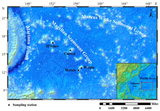
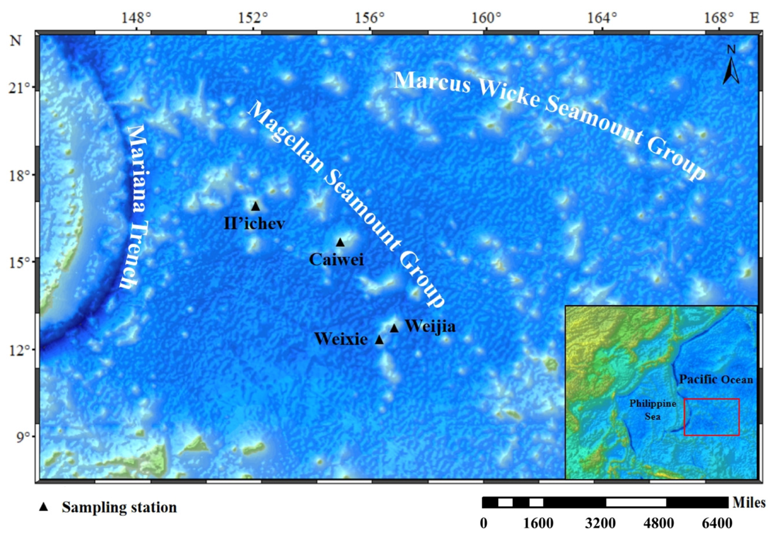
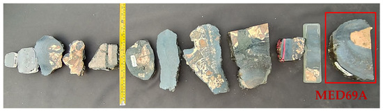
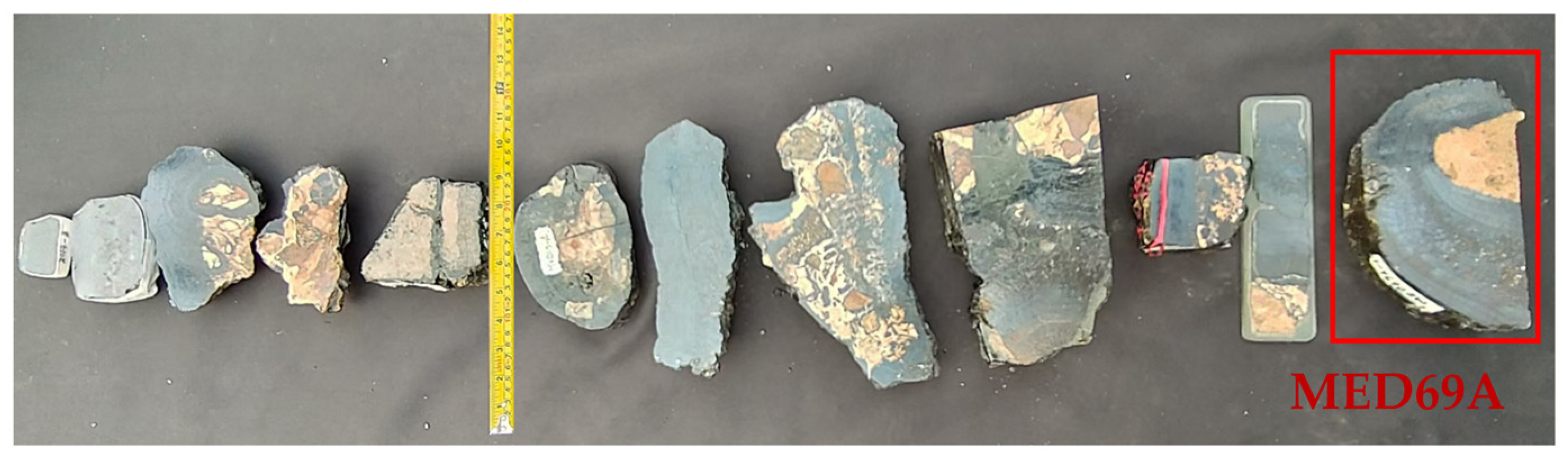
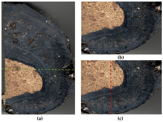
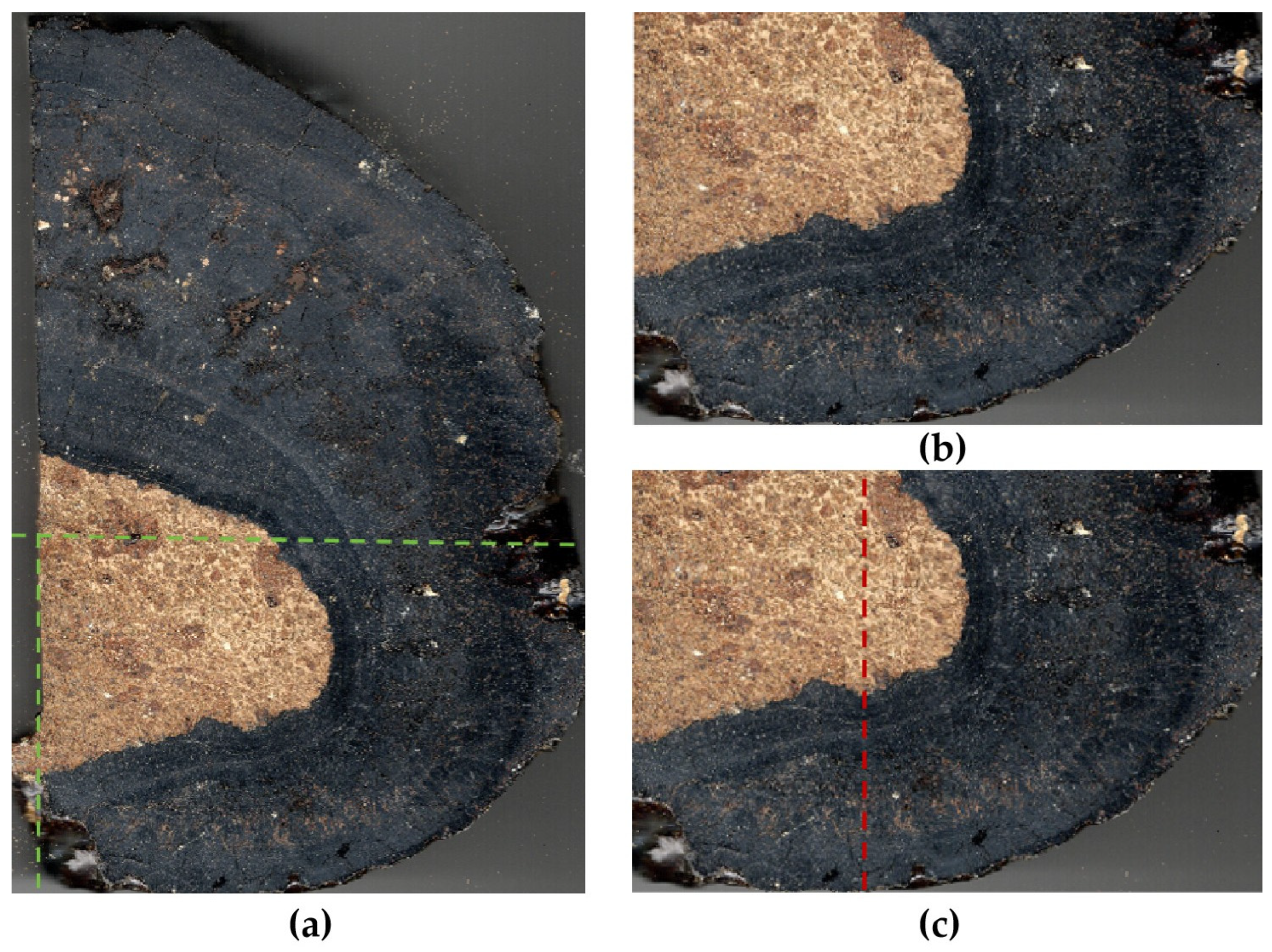
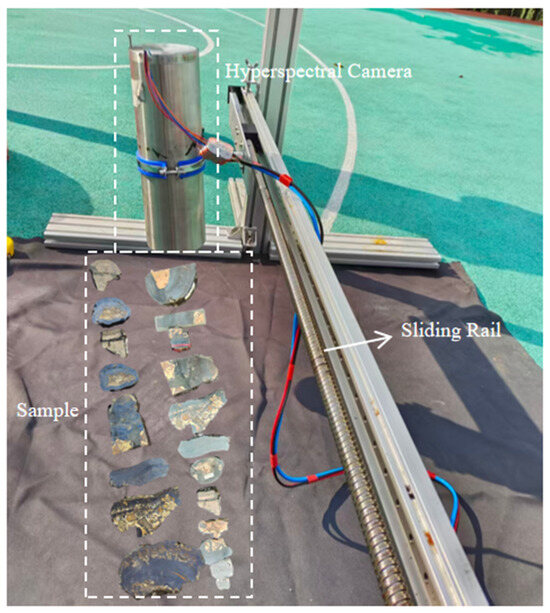
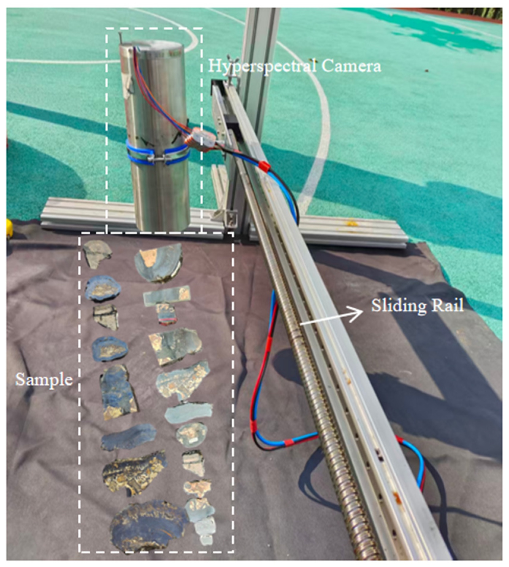
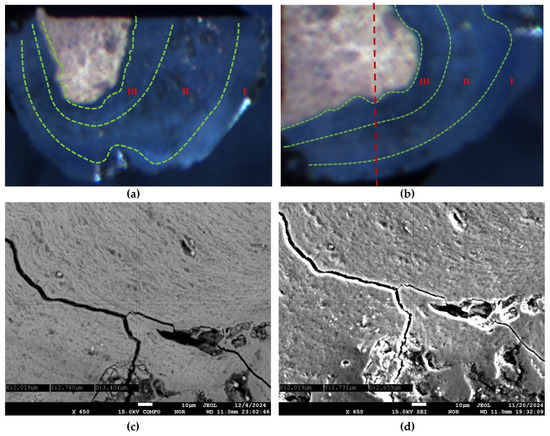
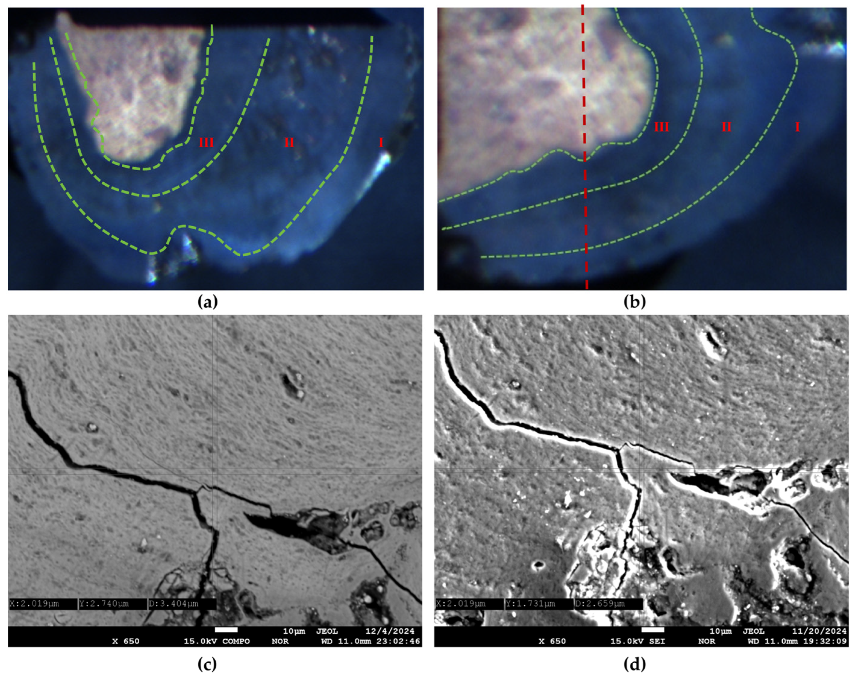
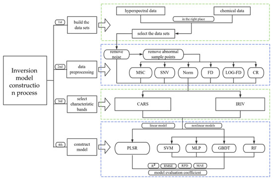
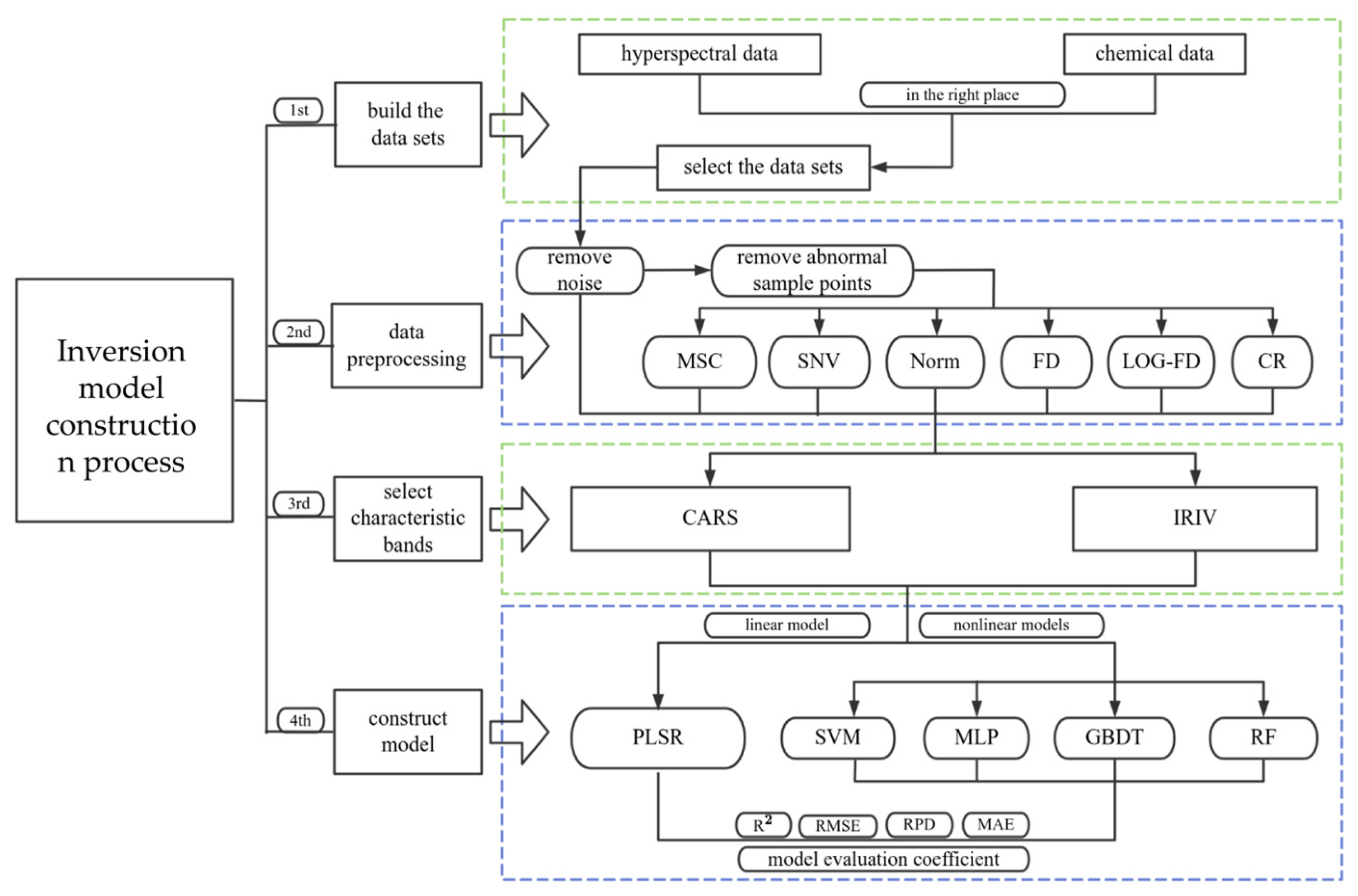
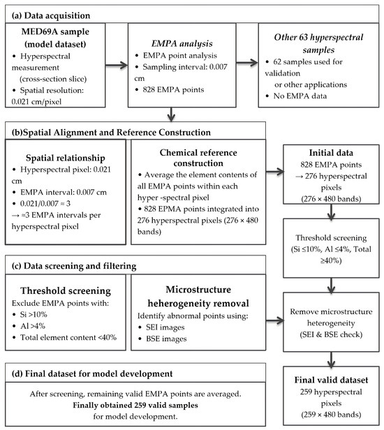
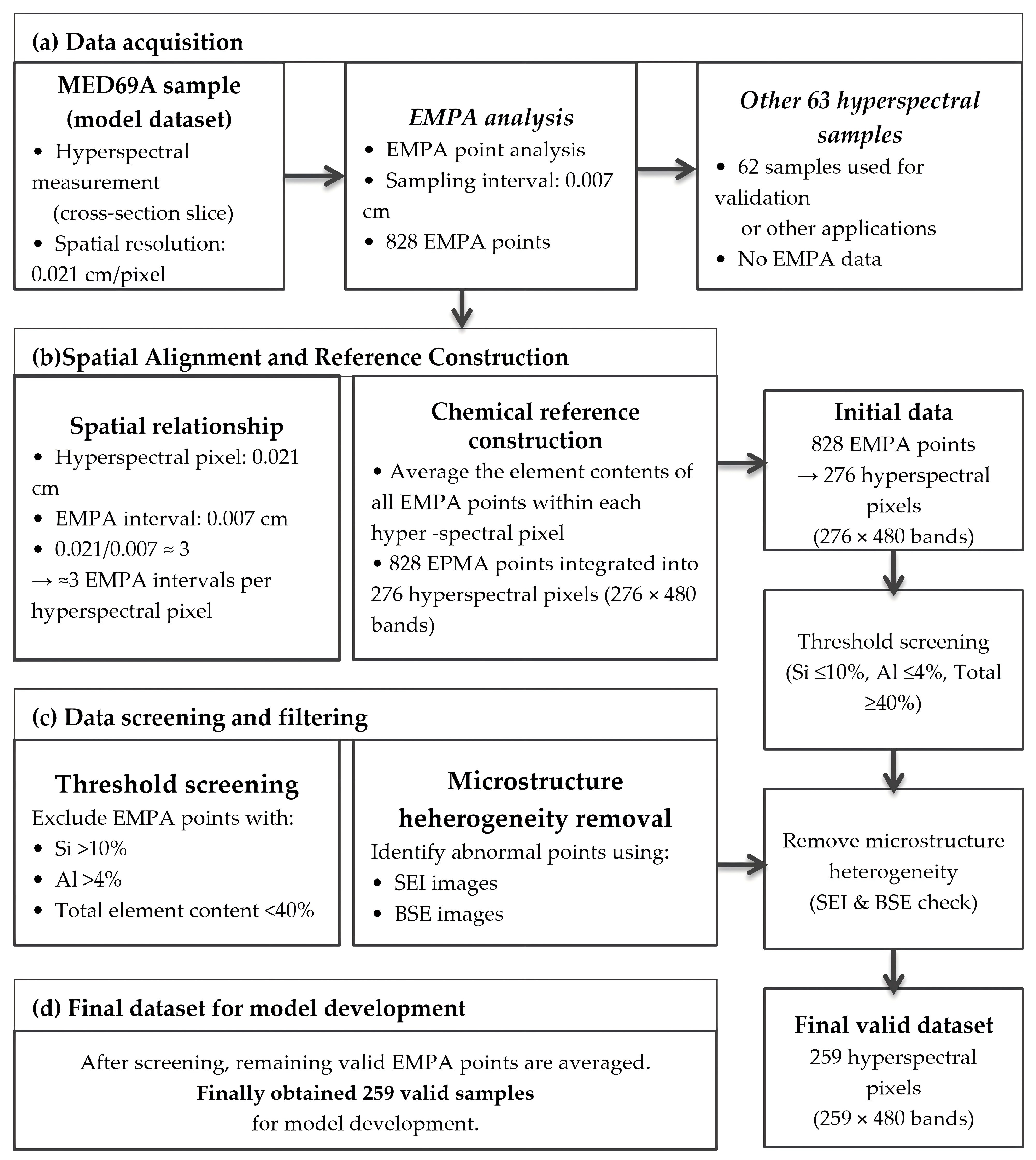
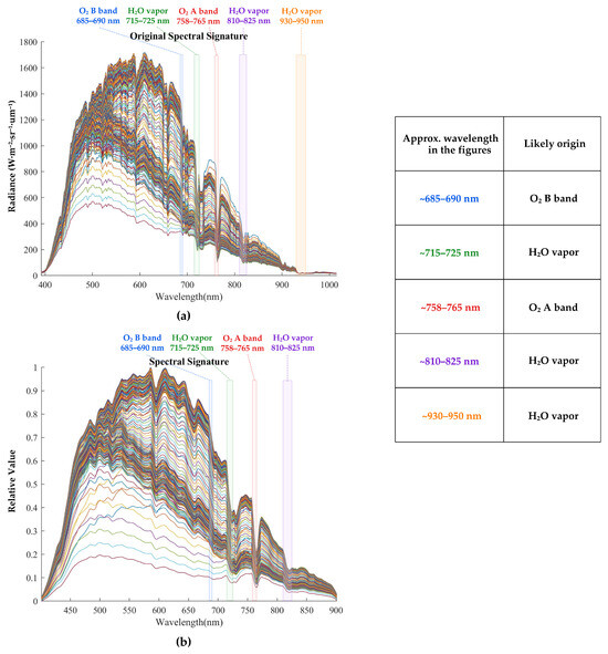
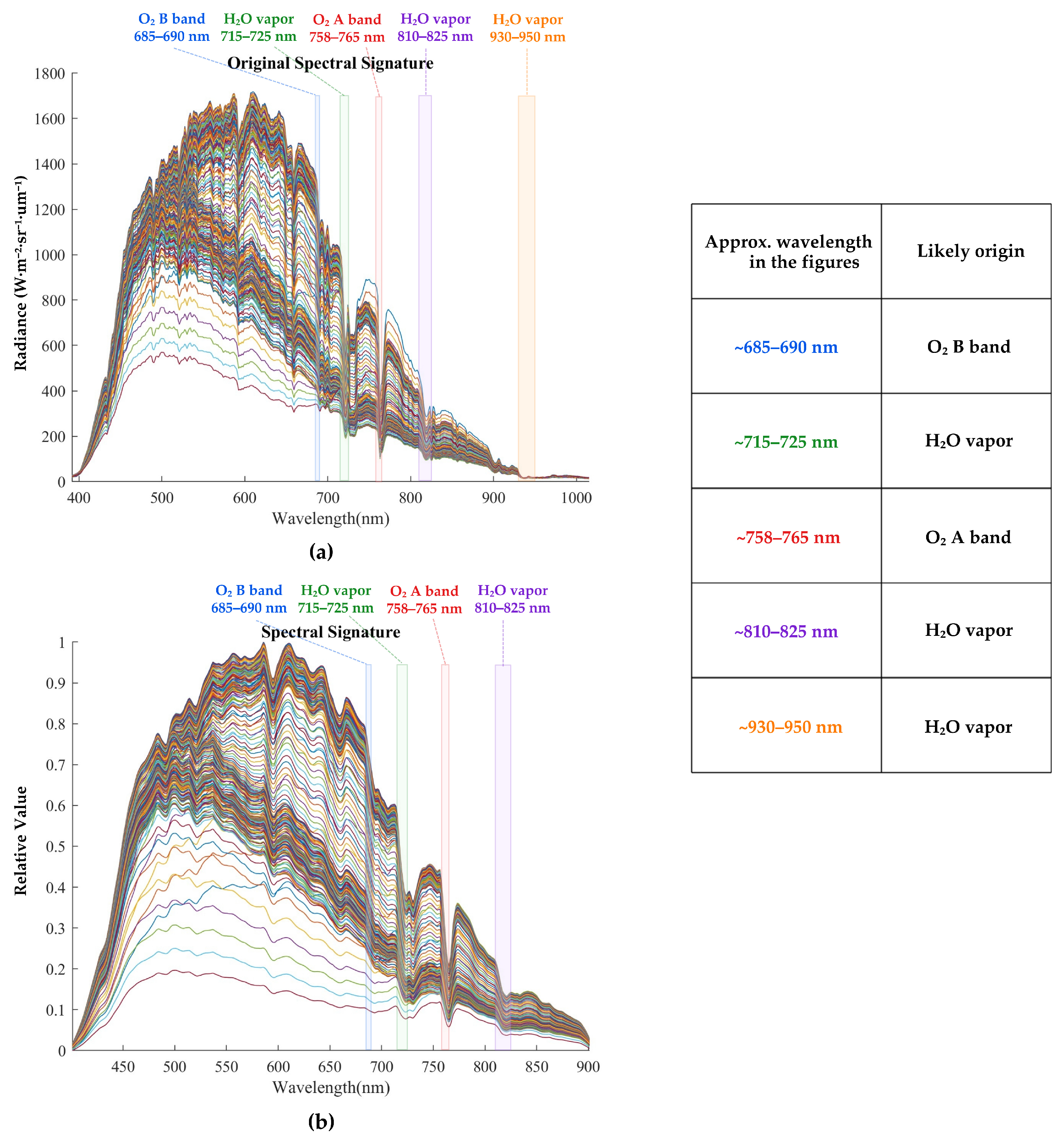
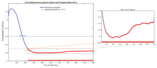
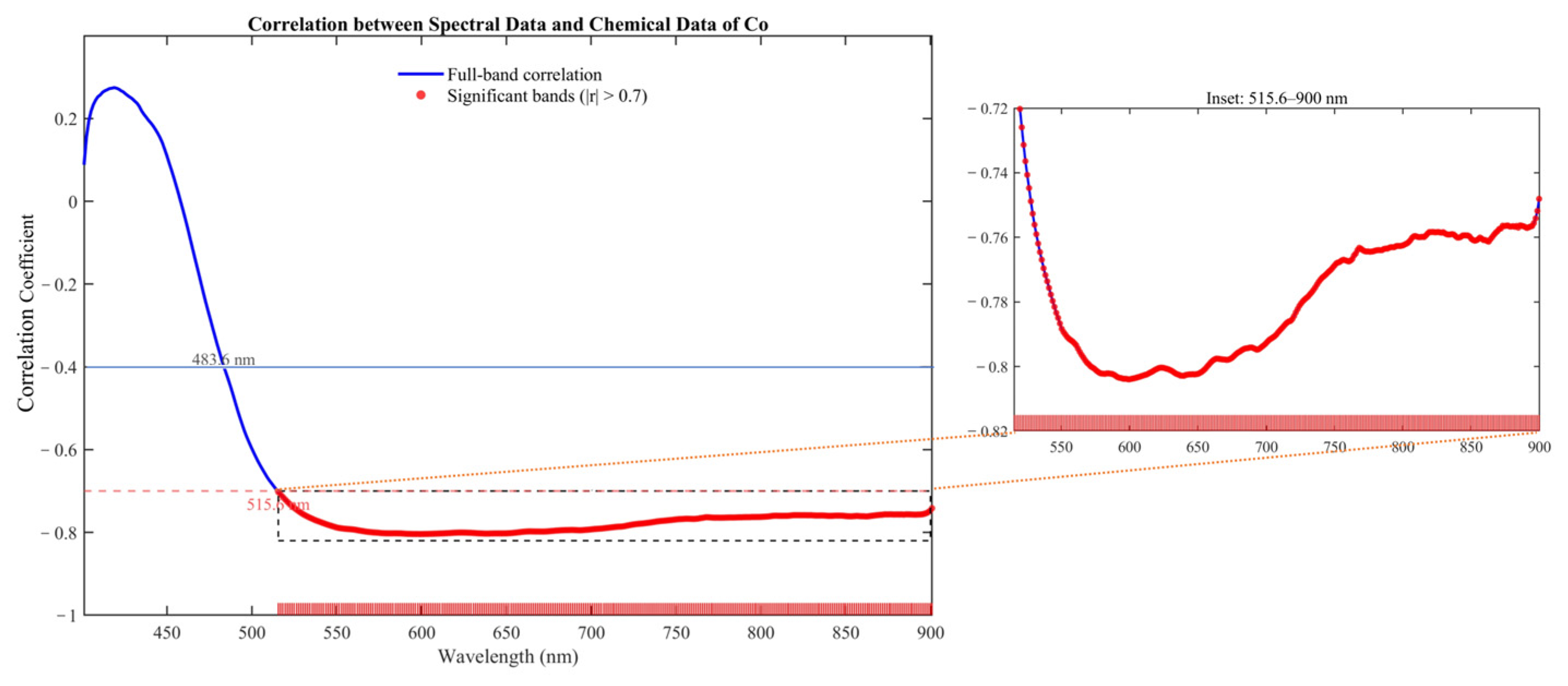
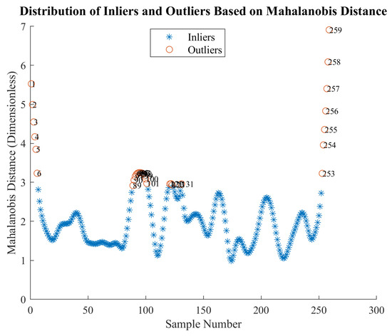
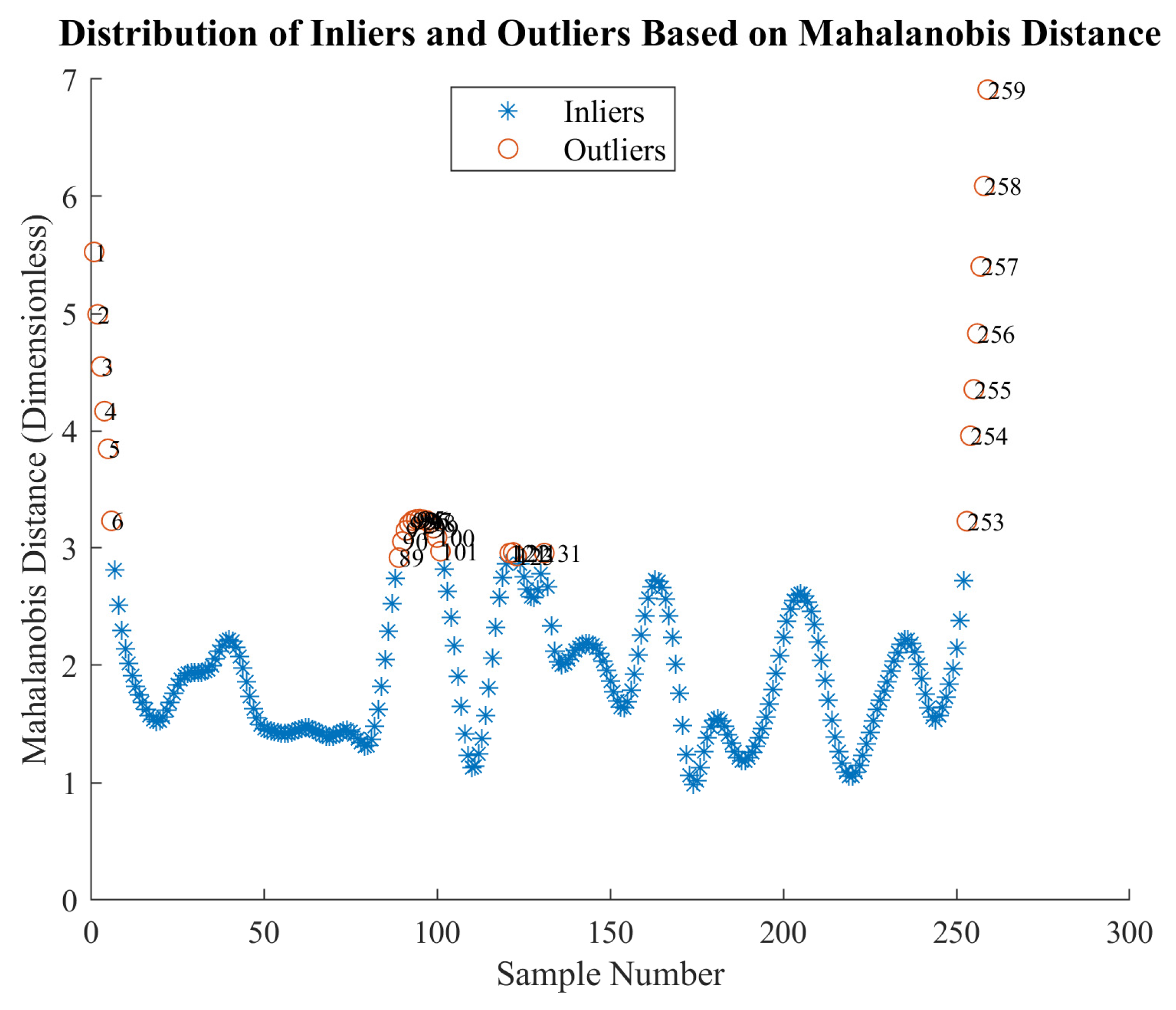
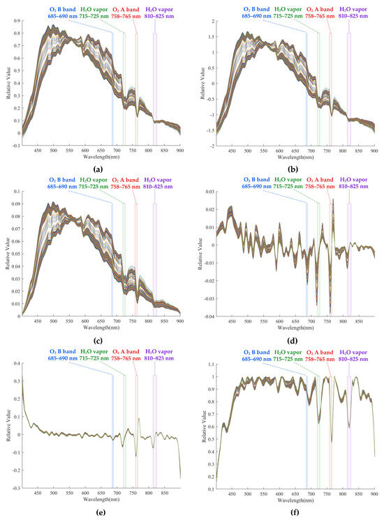
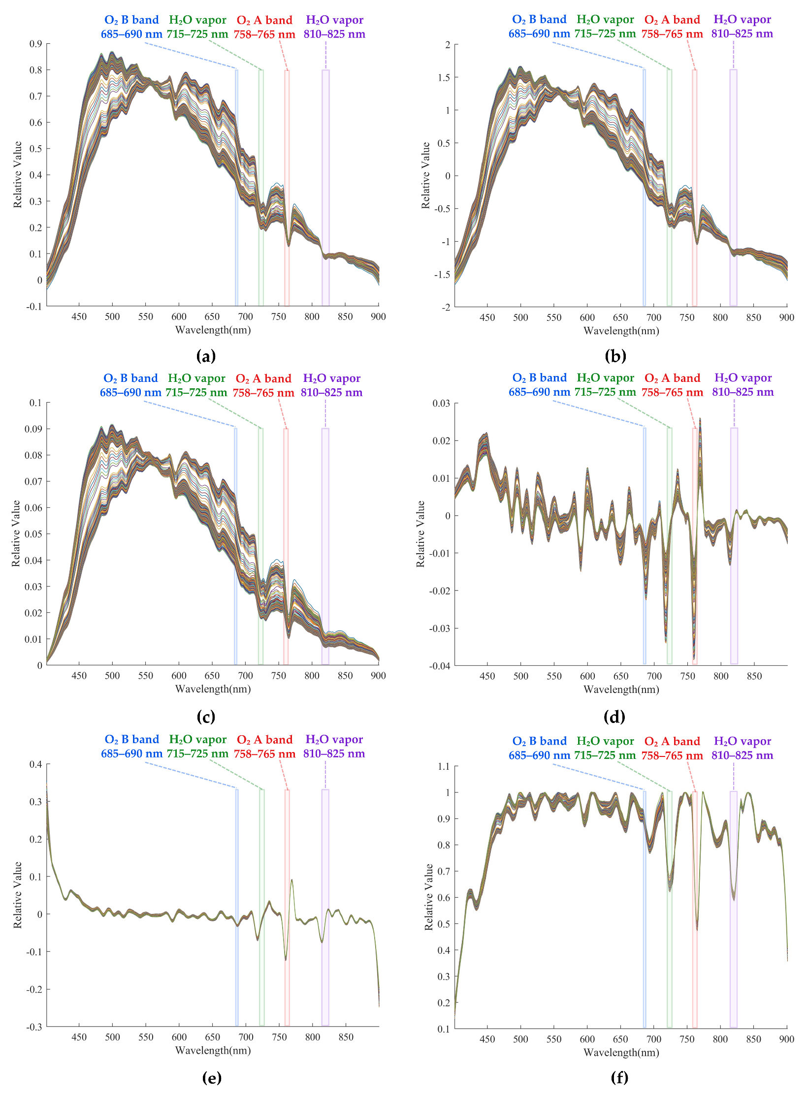
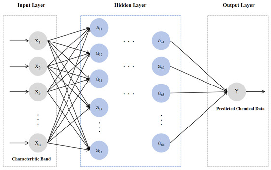
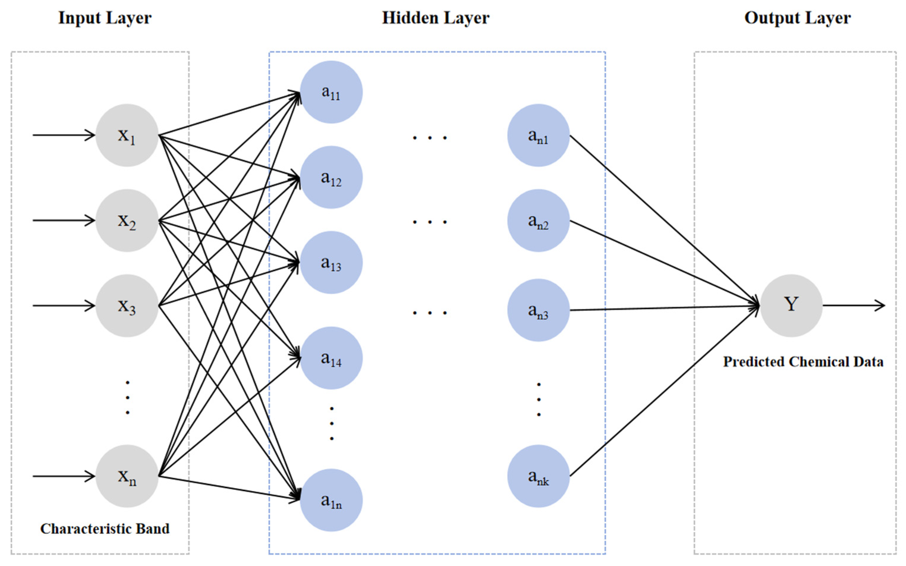
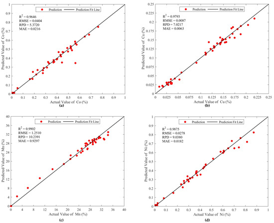
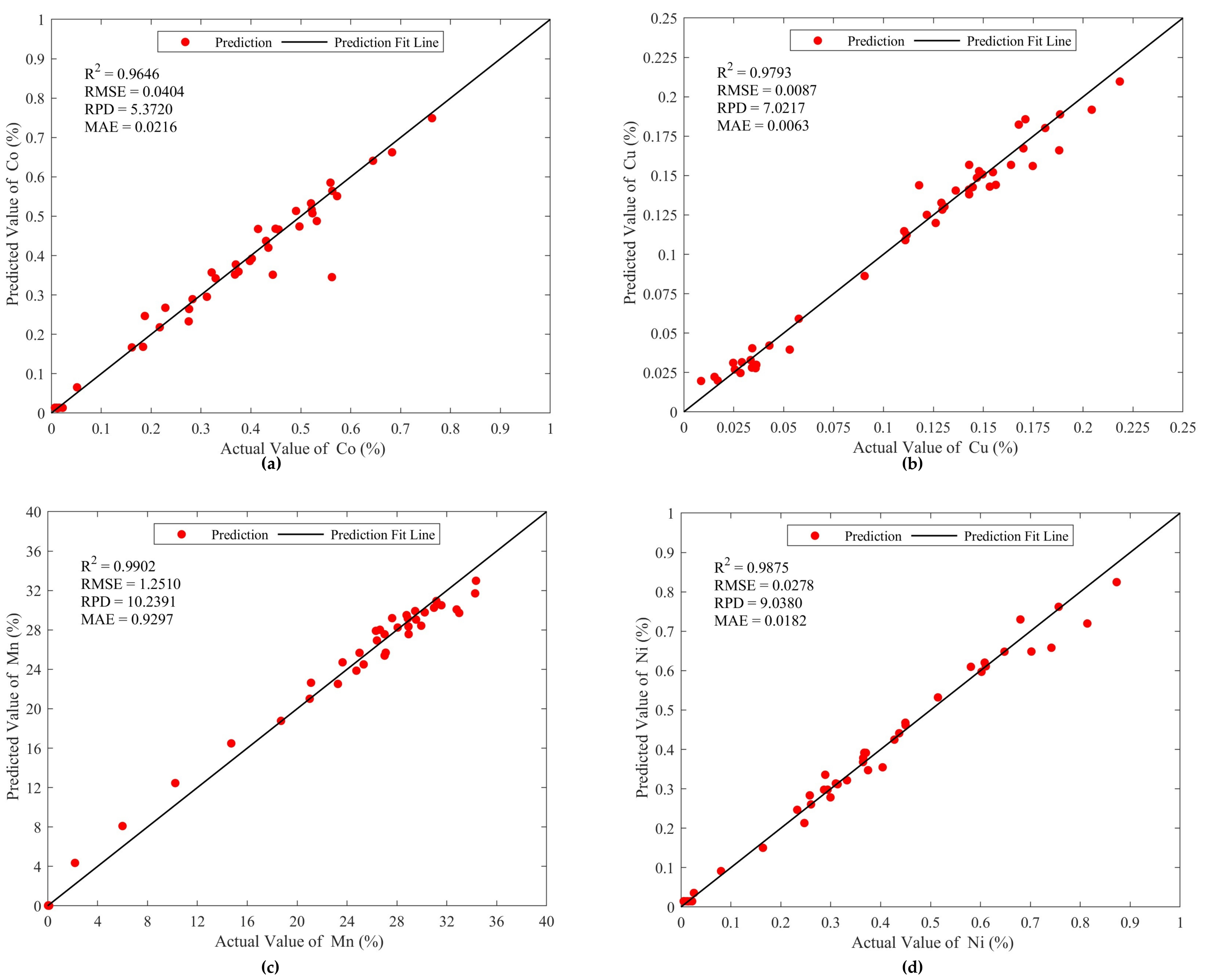
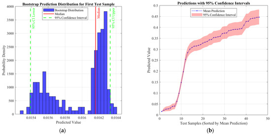
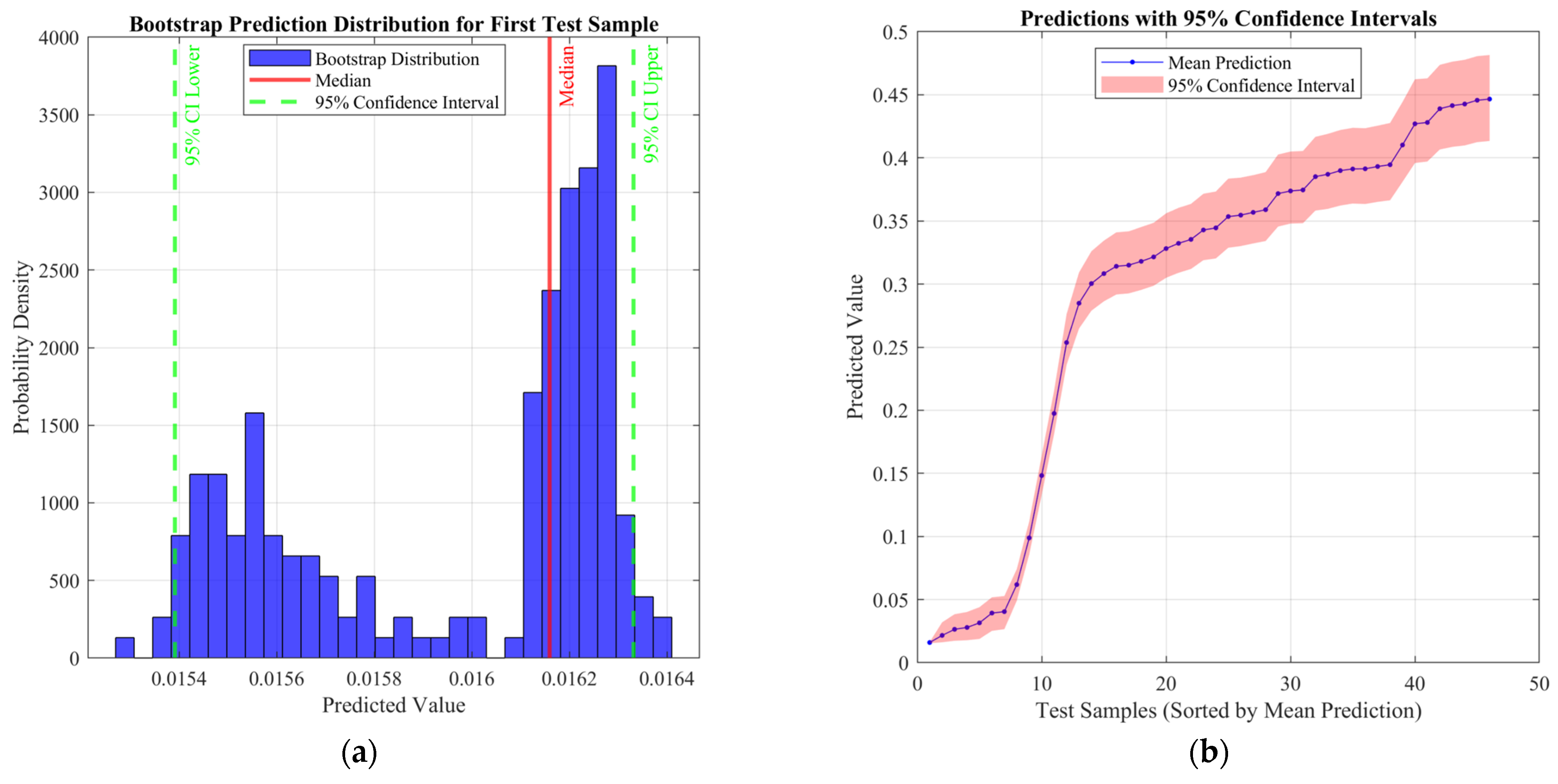
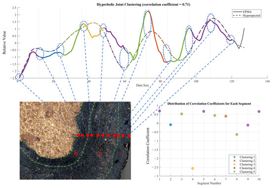
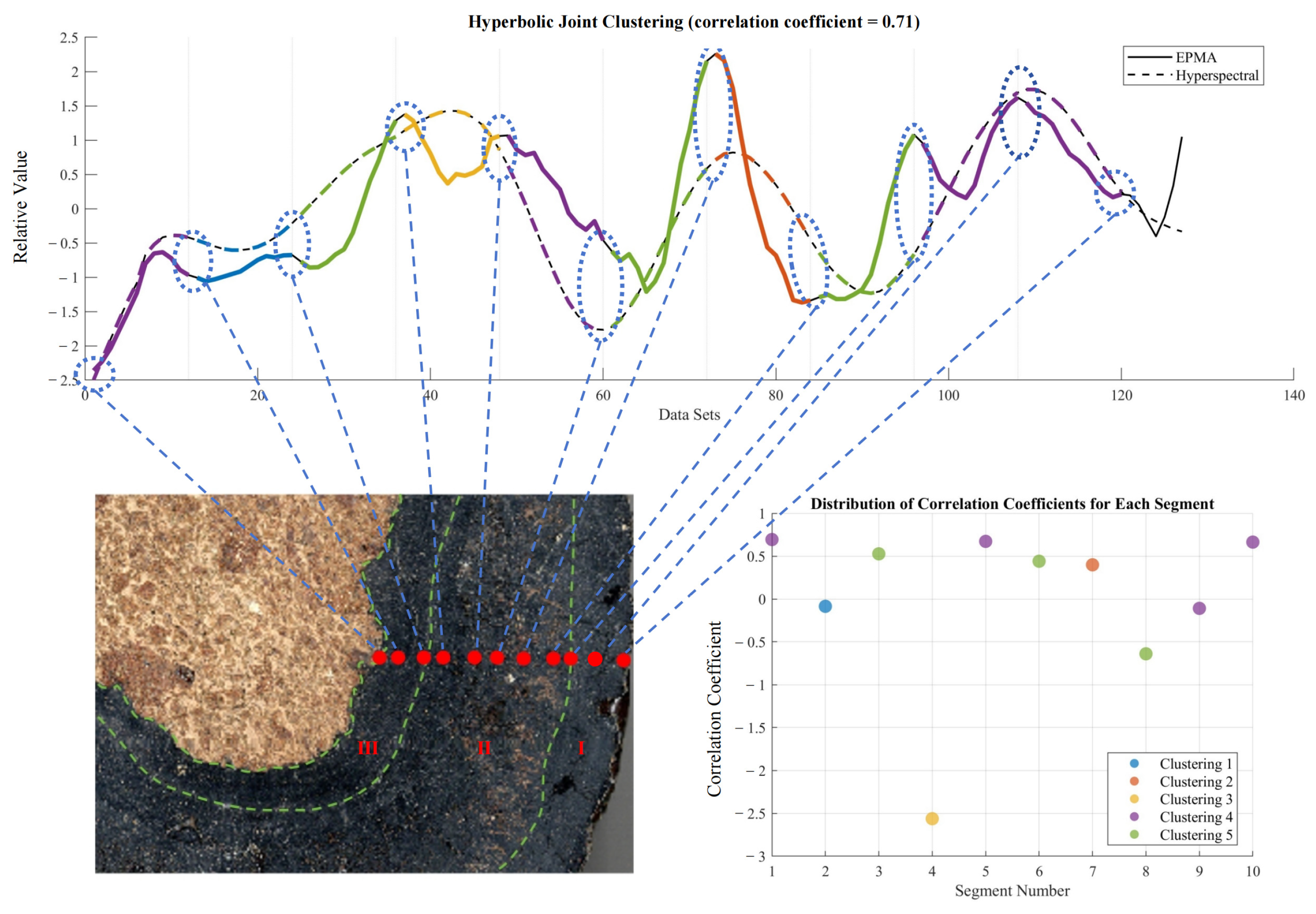
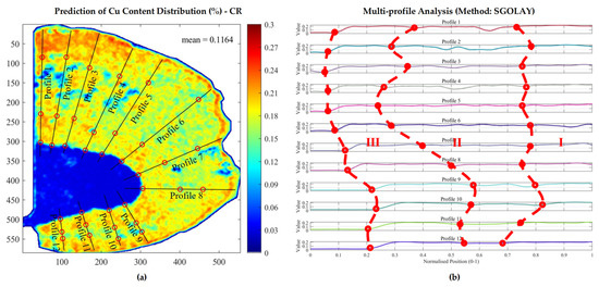
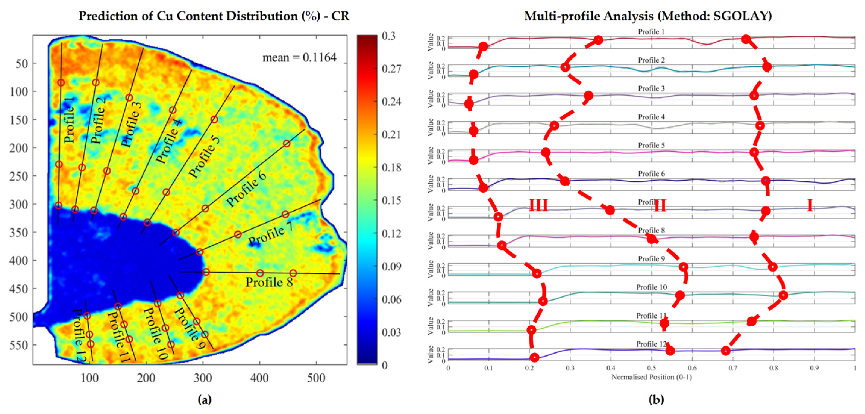

Disclaimer/Publisher’s Note: The statements, opinions and data contained in all publications are solely those of the individual author(s) and contributor(s) and not of MDPI and/or the editor(s). MDPI and/or the editor(s) disclaim responsibility for any injury to people or property resulting from any ideas, methods, instructions or products referred to in the content. |
© 2026 by the authors. Licensee MDPI, Basel, Switzerland. This article is an open access article distributed under the terms and conditions of the Creative Commons Attribution (CC BY) license.