


Highlights
What are the main findings?
- CSF processing transformed raw mobile CO2 observations into a more stable mapping target by suppressing transient positive peaks while preserving broader surface accumulation patterns.
- By combining CSF-processed mobile observations with multiscale remote sensing predictors, the proposed framework substantially improved surface CO2 prediction, achieving final R2 values of 0.90 in April and 0.93 in November.
What are the implications of the main findings?
- Mobile CO2 observations should be filtered and interpreted as stable surface concentration indicators rather than direct emission maps, reducing the risk of overinterpreting short-term traffic or plume disturbances.
- Integrating mobile monitoring, multiscale remote sensing predictors, spatial zoning, and SHAP interpretation provides an interpretable framework for refined urban carbon monitoring, hotspot diagnosis, and low-carbon urban planning.
Abstract
High-resolution mapping of urban surface CO2 is essential for refined carbon monitoring, emission management, and low-carbon urban planning. Mobile monitoring provides dense street-level observations, but raw CO2 measurements are often affected by transient traffic disturbances, vehicle idling, and localized plume events, which limits their direct use as stable spatial mapping targets. This study developed an integrated framework for predicting, mapping, and interpreting stable surface CO2 patterns in Shenzhen by combining vehicle mobile observations, CSF processing, multiscale remote sensing predictors, machine learning. A CSF-based lower-envelope filter was used to suppress short-duration positive peaks and extract a more stable CO2 accumulation signal from mobile observations. Multiscale predictors representing transportation, urban activity, surface environment, and built form were constructed to characterize both local and surrounding urban contexts. Compared with raw CO2, the CSF-processed target substantially improved prediction performance. The best validation R2 across the candidate models increased from 0.59 to 0.90 in April and from 0.62 to 0.93 in November. The predicted maps identified persistent high-CO2 areas in central and southwestern Shenzhen. SHAP results showed that transport networks and urban activity reinforced surface CO2 accumulation, whereas vegetation and open-surface contexts weakened accumulation at broader spatial ranges. These findings provide an interpretable framework for high-resolution urban CO2 mapping and refined low-carbon governance.
1. Introduction
High spatial resolution mapping of urban CO2 provides a critical basis for refined carbon governance and targeted mitigation. Urban areas are responsible for approximately 70% of global greenhouse gas emissions and account for nearly three quarters of global energy consumption, highlighting their critical role in achieving climate mitigation targets [1]. In China, the national goals of peaking CO2 emissions before 2030 and achieving carbon neutrality before 2060 have placed urban carbon governance at the center of climate policy implementation [2]. The transition from energy consumption control to the dual control of total carbon emissions and carbon intensity further emphasizes the need for spatially refined carbon monitoring and management [3]. Carbon related processes within cities exhibit strong spatial heterogeneity because transportation intensity, built environment characteristics, land use structure, commercial and residential activities, vegetation coverage, and industrial functions vary substantially across urban space [4,5]. Spatially continuous CO2 concentration information at high spatial resolution is essential for low-carbon transportation planning, low-carbon pilot evaluation, and refined urban carbon management [4,6].
Urban atmospheric CO2 has been investigated through satellite observations and fixed-site monitoring networks. Satellite observations provide broad spatial coverage and have substantially improved the characterization of regional and global atmospheric CO2 distributions [7,8]. Their application within cities remains constrained by retrieval resolution, spatial sampling density, cloud contamination, and revisit frequency. Fixed-site monitoring stations provide continuous temporal records and are valuable for characterizing long-term concentration variation, but their sparse spatial distribution limits their capacity to resolve street-scale differences across heterogeneous urban environments [7]. The contrasting strengths and limitations of these approaches leave an observational gap between broad-scale atmospheric CO2 monitoring and fine-scale characterization of concentration variability within cities.
Mobile CO2 monitoring has emerged as a promising approach for bridging the observational gap between large-scale atmospheric observations and localized urban carbon processes. By collecting high-density measurements along urban road networks, vehicle-based monitoring platforms provide surface CO2 observations at spatial resolutions that are difficult to achieve using satellite retrievals or fixed-site monitoring stations [9]. The extensive spatial coverage of mobile observations enables the characterization of diverse urban environments, including different road types, functional zones, and built-up settings [10]. Mobile measurements can capture spatial variations in CO2 concentrations associated with traffic activity, street canyon morphology, building density, vegetation exposure, and heterogeneous urban functions [11]. Consequently, mobile observations have become an important data source for investigating fine-scale spatial heterogeneity in urban CO2 distributions [12].
Despite their unique advantages, raw mobile CO2 observations cannot be directly interpreted as stable indicators of urban carbon intensity. Surface CO2 measurements collected along urban road networks reflect a combination of stable spatial signals and short-term concentration fluctuations [13]. In addition to the influence of underlying urban characteristics, observed concentrations can be strongly affected by transient emission events associated with traffic congestion, idling vehicles, heavy-duty trucks, intersections, restaurant exhausts, and parking garage outlets [14]. These short-duration concentration spikes may substantially increase spatial variability in mobile observations but do not necessarily represent stable differences in urban carbon environments. Consequently, machine learning models trained directly on raw CO2 observations may inadvertently capture temporary emission disturbances rather than stable spatial patterns [15]. Reducing the influence of transient concentration spikes therefore represents a critical prerequisite for deriving reliable indicators of urban CO2 spatial variability.
To better characterize persistent spatial patterns in urban CO2 distributions, transient concentration spikes embedded in mobile observations need to be distinguished from the underlying accumulation signal. Conventional smoothing approaches can reduce short-term fluctuations, but they may also blur genuine spatial gradients and weaken the representation of urban spatial heterogeneity [16]. A filtering strategy capable of suppressing localized concentration peaks while preserving broader spatial structure is therefore required. In this study, a Cloth Simulation Filter (CSF) was adopted to reduce the influence of transient concentration spikes and extract a more stable surface CO2 accumulation signal from mobile observations [17]. CSF approach can effectively suppress isolated peaks while maintaining the continuity of the underlying concentration surface, making it particularly suitable for highly heterogeneous urban CO2 observations [18]. The resulting signal is less sensitive to transient emission events, while retaining spatial patterns associated with urban morphology, transportation infrastructure, land use characteristics, and human activities. Rather than serving as a direct measure of carbon emissions, it provides an observation-based indicator of stable surface CO2 conditions and a more reliable target for subsequent spatial prediction and high-resolution mapping.
Spatial modeling of surface CO2 requires careful consideration of the spatial context in which concentrations are formed. CO2 observed at a given location is shaped by local sources, surrounding emission activities, atmospheric transport, urban morphology, vegetation exposure, and background concentration variability [11]. These processes indicate that CO2 variability cannot be fully explained by the land surface attributes of a single grid cell. Relevant spatial information may originate from multiple neighboring ranges, and different urban factors may operate over different spatial extents [19]. Traffic activity and road density may exert strong local influences [20], while land use composition, functional intensity, building morphology, and vegetation conditions may affect CO2 accumulation through broader neighborhood scale processes [10]. How to represent these multi range spatial effects and determine appropriate spatial contexts for different predictors remains insufficiently explored in high-resolution urban CO2 mapping. Multi source geospatial data can describe the spatial contexts associated with surface CO2 accumulation, including traffic related activity, urban functional intensity, socio economic activity, vegetation conditions, land cover composition, and built environment characteristics. Extracting these predictors across multiple spatial ranges allows both local and surrounding influences to be represented, providing a more appropriate basis for mapping stable surface CO2 signal.
This study focuses on Shenzhen, China, a rapidly urbanizing megacity characterized by heterogeneous urban forms and a growing demand for refined carbon governance. By integrating mobile CO2 observations with multi-source remote sensing data, this study aims to characterize stable spatial patterns of surface CO2 and provide observation evidence for refined urban carbon management. The main contributions of this study are as follows: (i) a CSF-based filtering strategy is introduced to reduce transient concentration spikes in mobile CO2 observations, thereby improving the suitability of mobile measurements for spatial mapping; (ii) a multiscale spatial representation framework based on multi-source remote sensing data is developed to characterize local and surrounding spatial contexts associated with surface CO2 variability; and (iii) high-resolution CO2 mapping is combined with spatial zoning and driver interpretation to identify high CO2 areas and support refined urban carbon governance, low-carbon transportation planning. The insights gained from Shenzhen may also help other rapidly urbanizing cities characterize fine-scale CO2 variability and identify CO2 accumulation areas.
2. Data
2.1. Study Area
Shenzhen is a highly urbanized megacity located in southern China and one of the core cities of the Guangdong-Hong Kong-Macao Greater Bay Area (Figure 1). In 2024, the city had a permanent population of 17.99 million and a gross domestic product of 3.68 trillion RMB, reflecting its high population density, strong economic activity, and intensive urban development [21]. Shenzhen has been widely recognized as a leading city in China’s low-carbon urban transition. It was selected as one of China’s first low-carbon pilot cities and has implemented a series of carbon governance measures, including carbon trading, transport electrification, green building development, carbon footprint certification, and the transition from energy consumption control to carbon emission dual control [22,23]. Shenzhen represents an important case for examining low-carbon urban transition, urban sustainability, and refined carbon governance in China. Rapid urbanization, intensive traffic activity, heterogeneous land use, dense built environments, and active low-carbon policy implementation are concentrated within a compact urban space, forming a spatially diverse and policy relevant context for high resolution surface CO2 mapping.
Figure 1.
Spatial distribution of mobile CO2 monitoring routes and observation platform in Shenzhen. (a) Spatial distribution of the monitoring routes during the April and November 2023 campaigns. (b) GAC AION Y electric vehicle used as the mobile observation platform. (c) Picarro G2301 analyser used to record CO2 concentrations.
2.2. Experimental Design
The mobile monitoring experiment was conducted using a GAC AION Y electric vehicle (GAC Aion New Energy Automobile Co., Ltd., Guangzhou, China) equipped with a Picarro G2301 analyser (Picarro, Inc., Santa Clara, CA, USA) and a GPS positioning device (Shandong Tianhe Environmental Technology Co., Ltd., Weifang, China). The electric vehicle platform was used to reduce interference from direct tailpipe emissions during measurements. The Picarro G2301 analyzer is a wavelength scanned cavity ring down spectroscopy (WS-CRDS) instrument, that acquires CO2 by utilizing an infrared spectrometer with a three-mirror cavity to analyze the decay rate profile of laser signals at wavelengths absorbed by the gas. These instruments were integrated on the vehicle platform to support synchronized acquisition of CO2 concentrations and spatial trajectories.
Two mobile CO2 monitoring campaigns were carried out in Shenzhen in 2023. The April campaign was conducted from 21 April to 28 April and collected 132,617 valid sampling records across six observation dates. The November campaign was conducted from 11 November to 17 November and collected 159,198 valid sampling records. The two campaigns were arranged along urban road networks to cover major urban districts in Shenzhen. The April campaign mainly covered Nanshan, Futian, Longgang, Dapeng, Luohu, Pingshan, and Yantian, while the November campaign covered Baoan, Guangming, Longhua, Longgang, Futian, Luohu, and Nanshan. The approximate route lengths were 386.58 km for the April campaign and 261.14 km for the November campaign. This experimental design provided dense street level CO2 observations across heterogeneous traffic environments, urban functions, and built environments, supporting high resolution mapping of surface CO2 spatial distribution in Shenzhen.
2.3. Multiscale Remote Sensing Predictors
Multiscale remote sensing predictors were constructed to represent the spatial context surrounding each mobile CO2 observation point. Surface CO2 is influenced by both local conditions and surrounding urban environments, so predictor variables were extracted across multiple spatial ranges rather than only from the grid cell where the observation was located. For each CO2 measurement point, square neighborhood windows were generated at 41 scale levels, including 0 m and 50 m to 2000 m at 50 m intervals. Statistical summaries of candidate predictors were calculated within each window to produce a multiscale representation of the surrounding urban environment. The final candidate predictor set contained 28 variables grouped into four categories: transportation, urban activity, surface environment, and built form (Table 1).
Table 1.
Multiscale remote sensing predictors for surface CO2 spatial modeling.
2.3.1. Transportation
Transportation predictors were constructed to describe road structure and transport infrastructure around each observation point. Road network data were obtained from OpenStreetMap (Figure 2e) and classified into six road types, including highway, main road, regional road, local road, nonmotorway, and rail. For each road type, the total road length within the neighborhood window was divided by the window area to calculate road length density, expressed as road length per square meter. Transport facility predictors were derived from AutoNavi POI data (Figure 2d). The numbers of parking lots, electric vehicle charging stations, gas stations, and public transportation facilities within each neighborhood window were divided by the window area to calculate facility densities, expressed as POI counts per square meter. These predictors were used to represent differences in traffic infrastructure, transport service intensity, and traffic related activity around the mobile CO2 observations.
Figure 2.
Multisource remote sensing datasets for deriving predictors in Shenzhen, China. Panels show (a) Sentinel-2 RGB imagery, (b) SDGSAT-1 nighttime light, (c) ESA WorldCover land cover, (d) AutoNavi POIs, (e) OpenStreetMap road network, and (f) CNBH 10 m building height.
2.3.2. Urban Activity
Urban activity predictors were derived from nighttime light data and points of interest (POIs). the level of urban development is characterized by the intensity of nightlights, which are obtained from SDGSAT-1 satellite Glimmer Imager for Urbanization (GIU; Changchun Institute of Optics, Fine Mechanics and Physics, Chinese Academy of Sciences, Changchun, China), at a10 m resolution (Figure 2b). The nightlight imagery used in this study was captured on 28 December 2023, and radiometric calibration was conducted to ensure the highest quality and reliability of the data [24]. Features related to urban functions are derived by analyzing and processing data on POIs collected from AutoNavi maps (Figure 2d). POIs are categorized into eight groups: residence communities, life services, office space, medical/education, government, entertainment, commercial services, and others. After excluding the “others” category, we used the density of the remaining categories to represent the urban functional characteristics of areas near observation points. Additionally, to quantify land use diversity, we computed a mixed land use index based on the number of each category of POIs, reflecting the richness and balance of land use in the area. This study employs the Shannon–Wiener Diversity Index, a widely used measure to assess mixed urban land use [25]. The formula for this index is
where represents the number of POI categories ( = 7), and is the proportion of the -th POI among all POIs.
2.3.3. Surface Environment
Surface environment predictors are represented by spectral indices and the proportions of different land use classifications. Normalized Difference Vegetation Index (NDVI), and Normalized Difference Water Index (NDWI) were calculated separately for the April and November campaigns from median Sentinel-2 surface reflectance composites. Figure 2a presents the Sentinel-2 RGB composite for November 2023. The image acquisition and processing were completed on the Google Earth Engine platform using the Level 2A surface reflectance product, which has been corrected for geometry, radiometry, and atmosphere using Sen2Cor (version 2.10). Moreover, the ESA WorldCover 10 m 2021 v200 dataset (Figure 2c) [26] was used to calculate the proportions of vegetation, bare soil, water, and building to further describe the environmental characteristics near observation points.
2.3.4. Built Form
Built form predictors were constructed to describe the three-dimensional structure of the built environment. Building density (BD), average building height (AH), and building volume ratio (BVR) were calculated within each spatial range using the CNBH 10 m building height dataset (Figure 2f) [27]. BD was defined as the proportion of building footprint area within the neighborhood window:
AH was calculated as the mean height of building pixels:
BVR was calculated as the window mean building height normalized by the reference maximum building height:
where is the number of building pixels within the neighborhood window, is the total number of pixels within the neighborhood window, is the height of the -th building pixel, and is the reference maximum building height. BD represents the horizontal coverage of buildings, AH describes the mean vertical height of building pixels, and BVR characterizes the normalized three-dimensional building intensity within the neighborhood window.
3. Methodology
3.1. Methodological Framework
Figure 3 illustrates the methodological framework for high resolution mapping and interpretation of stable urban surface CO2 Concentration Patterns. The framework contains two parallel data branches. Mobile CO2 observations are processed using a CSF lower envelope filter to suppress transient positive peaks and obtain a stable modeling target. In parallel, multisource remote sensing data are used to construct predictors representing transportation, urban activity, surface environment, and built form across multiple spatial ranges.
Figure 3.
Methodological framework for mapping and interpreting stable urban surface CO2. The asterisk is part of the standard notation for the Getis-Ord Gi* statistic.
The filtered CO2 target and multiscale predictors are jointly used in the scale response analysis. Predictor responses are evaluated at the self, local, block, and background ranges to identify the most informative spatial scales. The selected predictors are then screened using Variance Inflation Factor (VIF) analysis and recursive feature elimination. Four machine learning models are developed and evaluated using spatial validation based on 500 m grid cells, and the optimal predictor subset and model are selected.
The selected model is used to generate 10 m resolution maps of stable surface CO2. Jenks natural breaks and Getis Ord Gi* analysis are applied to identify spatial accumulation patterns, while SHAP analysis is used to interpret the contribution and effect direction of the selected predictors. The framework therefore connects stable signal extraction, multiscale predictor construction, scale selection, predictor screening, spatial prediction, zoning, and driver interpretation within a unified analytical process.
3.2. Filtering of Mobile CO2 Observations
The CSF was adapted from the cloth simulation filtering method originally proposed for three-dimensional airborne LiDAR point cloud filtering [17]. In the original CSF method, the point cloud is inverted, and a virtual cloth is allowed to fall onto the inverted surface to approximate the ground surface. Following this idea, the observed CO2 series was first inverted in this study, and a virtual cloth was allowed to move toward the inverted concentration surface under gravity and continuity constraints. After transforming the final cloth surface back to the original CO2 scale, the simulated cloth provided a lower-envelope estimate of the observed concentration series.
Before filtering, valid CO2 observations were grouped by observation date and sorted by time. To avoid applying the filter across discontinuous trajectories, each daily sequence was further divided into shorter time segments. A new segment was created when the time gap between two adjacent observations exceeded 5 min or when the duration of the current segment exceeded 30 min. The CSF was then applied independently to each segment. For each continuous time segment, the observed CO2 sequence was treated as a one-dimensional profile along the normalized time coordinate. The cloth node position was updated as:
where is the predicted vertical position of the i-th cloth node before contact and stiffness constraints, is the corrected cloth node position at iteration k, γ is the damping coefficient, g is the gravity parameter, and τ is the time step. The adapted filter used here operates on a one-dimensional cloth curve in the x-z plane. After the motion prediction, contact constraints with the inverted CO2 surface and stiffness constraints between adjacent and second-order neighboring nodes were applied to maintain curve continuity and prevent the cloth from being pulled excessively by isolated concentration peaks. After all iterations, the resulting lower-envelope signal was used as the filtered CO2 observation. Four CSF parameter settings were tested to examine the sensitivity of the filtering strength: soft, balanced, stiff, and tight. Softer settings allow the cloth to follow local variations more closely, while stiffer settings impose stronger continuity constraints and produce a smoother lower-envelope signal. The selected CSF-processed CO2 signal was used as the target variable for subsequent high-resolution mapping.
To examine whether the CSF provided a more appropriate target signal for mobile CO2 mapping, four commonly used filtering methods were implemented for comparison: locally weighted scatterplot smoothing (LOWESS), moving quantile filtering, robust spline smoothing, and Haar wavelet filtering. LOWESS estimates a continuous local trend using neighboring observations and is useful for preserving gradual variations [28]. Moving quantile filtering emphasizes the lower portion of the concentration distribution within a moving window, making it less sensitive to short-term positive spikes [29]. Robust spline smoothing fits a smooth baseline while reducing the influence of outliers [30]. Haar wavelet filtering decomposes the signal into low-frequency and high-frequency components, allowing high-frequency fluctuations to be suppressed [31].
The filtering performance of the four conventional methods and four CSF configurations was quantitatively evaluated using all valid observations from the two campaigns. Let denote the observed concentration, the filtered baseline, and the number of valid samples. Four complementary indicators were calculated:
Here, measures baseline roughness, measures lower-envelope violations, SDR represents the ratio of the standard deviation after filtering to that before filtering, and measures peak reduction based on the 95th percentile. These indicators were evaluated jointly to assess baseline smoothness, lower-envelope compliance, signal retention, and suppression of positive concentration enhancements.
3.3. Scale-Dependent Response of Urban Predictors
Surface CO2 concentrations can be associated with urban environments over different spatial extents, because traffic infrastructure, urban activity, surface composition, vegetation coverage, and building morphology may influence emissions, dispersion, and surface exchange at different ranges. Scale-response analysis was therefore conducted separately for the April and November campaigns. Each predictor was evaluated from 0 to 2000 m at 50 m intervals, producing 41 candidate spatial scales. These scales were grouped into four predefined ranges. The point scale at 0 m represented conditions at the observation location. The local range from 50 to 500 m represented the immediate surroundings, the block range from 550 to 1200 m represented the intermediate urban context, and the background range from 1250 to 2000 m represented broader surrounding conditions. For each predictor, the optimal scale was selected within each predefined spatial range to retain information from point, local, block, and background contexts. This range selection avoids the loss of scale-dependent responses associated with using a single global optimum and provides a more complete multiscale representation of urban influences on surface CO2.
The CSF-processed CO2 concentration was used as the response variable, and the response strength between each predictor and surface CO2 was evaluated using two complementary metrics: the absolute Spearman correlation coefficient and normalized mutual information. The absolute Spearman correlation coefficient was used to measure monotonic association, which is suitable for identifying whether CO2 tends to increase or decrease consistently with a predictor [32]. Normalized mutual information was used as a complementary dependence metric to capture broader statistical associations, including potential nonlinear and non-monotonic relationships that may not be fully represented by monotonic association [33]. The two metrics were combined into an overall response score:
where represents the integrated response strength at scale s, is the absolute Spearman correlation coefficient at scale s, and is the normalized mutual information at scale s.
A spatially balanced Monte Carlo sampling strategy was used to reduce the influence of uneven mobile sampling density. The study area was divided into 2000 m × 2000 m grid cells, and one observation was randomly selected from each grid cell containing valid samples during each repetition. Response scores were then calculated for every predictor at all candidate scales using the spatially balanced subset. This procedure was repeated 100 times with a fixed random seed, and the mean response score across the repetitions was used to select the optimal scale within each predefined spatial range. For each predictor, the scale with the highest mean response score was selected within each range, and a global best scale was identified. The selected combinations were subsequently included in VIF screening and recursive feature elimination.
3.4. Machine Learning Models and Spatial Validation
Four tree-based models, including random forest (RF), extreme gradient boosting (XGBoost), CatBoost, and LightGBM, were used to predict the CSF-processed surface CO2 concentration. These models were selected because of their strong predictive capacity for nonlinear and heterogeneous relationships between multiscale urban predictors and CO2 concentrations [10,34,35]. The April and November datasets were modeled separately to evaluate predictive performance under different observation periods. In addition to the multiscale urban predictors, observation time was included as a fixed predictor in all models to account for within-day temporal variation.
To reduce spatial leakage between training and validation samples, a grid-based spatial validation strategy was adopted. The coordinates of all samples were divided into 500 m × 500 m grid cells. The train–validation split was performed using grid cells as groups, with 20% of the grids assigned to the validation set and the remaining grids used for model training. This design ensured that samples from the same 500 m grid cell were not simultaneously used for training and validation.
Model performance was evaluated using three metrics: coefficient of determination (R2), root mean square error (RMSE), and mean absolute error (MAE).
where n represents the number of testing samples, the -th predicted value, the -th measured CO2 concentration, and the average CO2 concentration in the testing set.
3.5. Collinearity Control and Optimal Predictor Subset Selection
Before model-based feature selection, variance inflation factor (VIF) screening was used to control multicollinearity among the multiscale predictors. VIF measures the extent to which the information carried by one predictor can be linearly explained by the remaining predictors. Predictors with high VIF values provide limited independent information and may introduce redundancy into the model. Therefore, variables were iteratively removed according to their VIF values until all retained predictors showed acceptable collinearity, with the maximum VIF constrained to 10 [36].
After VIF filtering, recursive feature elimination (RFE) was used to determine the optimal predictor subset for each month and model. Starting from the VIF-retained predictors, the model was repeatedly trained on the current feature subset. At each step, model performance was evaluated on the validation set, and the least important predictor was excluded according to the feature importance. This procedure continued until five removable predictors remained. The optimal feature combination was selected as the subset with the lowest validation MAE.
3.6. High-Resolution Mapping of CSF-Processed Surface CO2
After model training, spatial validation, and optimal predictor subset selection, the best-performing model for each campaign was used to generate spatially continuous maps of CSF-processed surface CO2 concentrations. The mapping was conducted at a spatial resolution of 10 m to maintain consistency with the native spatial resolution of the remote sensing datasets. For each campaign, the selected predictors were prepared at the mapping resolution. Observation time was included as a dynamic input variable to represent intraday variation during the mobile monitoring periods. Four daytime periods were mapped according to the temporal coverage of the mobile monitoring campaigns, including 08:00–10:00, 10:00–12:00, 14:00–16:00, and 16:00–18:00. Within each two-hour period, predictions were generated at 10 min intervals and then averaged to obtain the CO2 map. The overall daytime mean map was calculated by averaging the four period maps.
4. Results
4.1. Comparison of Filtering Strategies for Mobile CO2 Observations
This section evaluates the filtering behavior of conventional methods and the CSF lower-envelope approach, with emphasis on peak suppression, baseline continuity, and variability retention. An illustrative segment of mobile CO2 observations collected in Futian District on 12 November 2023 between 15:00 and 15:30 was selected to compare the behavior of different filtering methods (Figure 4). This segment contains typical characteristics of urban mobile CO2 measurements, with frequent short-term positive fluctuations superimposed on a gradually varying concentration pattern. The coexistence of sharp local peaks and broader baseline variation indicates that the raw observations include both transient disturbances and relatively stable spatial signals, supporting the need for filtering before spatial modeling. To complement this segment-level comparison, the filtering performance of the four conventional methods and four CSF configurations was quantitatively evaluated using all valid observations from April and November, as summarized in Table 2.
Figure 4.
Comparison of conventional filtering methods and CSF configurations for mobile CO2 observations. Panels (a,c) show the filtered CO2 baselines derived from conventional methods and CSF configurations, respectively. Panels (b1–b4,d1–d4) show the corresponding residuals, calculated as observed CO2 minus the filtered baseline. The example sequence was extracted from mobile CO2 observations collected in Futian District, Shenzhen, between 15:00 and 15:30 on 12 November 2023.
Table 2.
Full-dataset quantitative comparison of conventional filtering methods and CSF configurations in April and November 2023.
The conventional filtering methods showed different responses to short-term CO2 fluctuations. LOWESS produced a smooth and continuous baseline, but it was still partly influenced by strong positive peaks, causing the estimated baseline to rise during abrupt concentration enhancements. Moving Quantile filtering was more effective in suppressing high concentration spikes and generated a lower baseline, but its local-window calculation led to relatively abrupt changes in some segments. Robust Spline also provided a continuous baseline and reduced part of the influence of outliers, although strong peaks still affected the fitted curve. Haar Wavelet filtering reduced high-frequency fluctuations, but its stepwise baseline was less consistent with the gradual variation expected along the mobile trajectory. The full-dataset evaluation showed that the conventional methods had violation rates of 35.32% to 51.10% in April and 32.96% to 59.39% in November, indicating frequent departures from the lower-envelope requirement. Moving Quantile achieved the greatest peak reduction among the conventional methods, but it also produced the highest April roughness. Robust Spline produced relatively low roughness, but its violation rates exceeded 50% in both campaigns. Thus, none of the conventional methods simultaneously achieved lower-envelope compliance, baseline continuity, and effective peak suppression.
The CSF processing results showed a more stable lower-envelope behavior. Across the four CSF configurations, the estimated baselines remained below the raw observations and followed the broader variation in the CO2 sequence without being strongly affected by isolated positive peaks. The soft setting was more responsive to local changes, whereas the stiff and tight settings imposed stronger continuity constraints and produced smoother lower-envelope estimates. All four CSF configurations achieved a violation rate of 0% in both campaigns. From the soft to tight settings, roughness decreased from 2.891 to 2.314 in April and from 0.561 to 0.369 in November, while peak reduction increased from 0.76% to 1.29% and from 6.16% to 8.15%, respectively.
The stiff configuration was selected because it provided the most suitable balance across the four evaluation criteria. Relative to the balanced setting, it reduced roughness from 2.661 to 2.525 in April and from 0.412 to 0.381 in November, while increasing peak reduction from 1.08% to 1.20% and from 7.42% to 7.85%, respectively. The tight setting provided only marginal additional improvements in roughness and peak reduction. Its SDR was also only slightly lower than that of the stiff setting, changing from 0.924 to 0.923 in April and from 0.492 to 0.480 in November. The stiff configuration therefore improved baseline continuity and peak suppression while retaining slightly more overall concentration variability than the tight setting. The resulting CSF-processed CO2 series was used as the target variable in the subsequent scale response analysis, feature screening, and spatial modeling.
4.2. Multiscale Responses and Predictor Selection
Table A1 summarizes the optimal response scales of all candidate predictors in the April and November campaigns, including the point, local, block, background, and global best scales. Figure 5 presents the scale–response curves of four representative predictors, including main road density, nightlight, vegetation percentage, and building density, allowing direct comparison of their response strength and optimal scales between the two campaigns.
Figure 5.
Scale-dependent response scores and optimal buffer scales of representative urban predictors for surface CO2 modeling: (a) main road density; (b) nightlight; (c) vegetation percentage; and (d) building density.
Across both campaigns, most predictors showed stronger responses beyond the point scale. The background range contained the global best scales of 25 of the 28 candidate predictors in April and 24 of the 28 predictors in November, demonstrating a common dependence on the broader urban environment (Table A1). Despite this general pattern, individual predictors showed different degrees of change between the two campaigns. The global best scale of main road density changed only slightly from 1300 m in April to 1350 m in November, while that of nightlight changed from 1550 to 1400 m. More substantial changes were observed for office space, which shifted from 900 to 1800 m, and for NDVI, which shifted from 1950 to 150 m.
Figure 5 provides a complementary view of these differences by showing how the response strength of representative predictors changed across buffer scales. Main road density and nightlight showed stronger responses at broader scales, especially in the April campaign, suggesting that transportation structure and urban activity intensity influenced CO2 variability beyond the immediate observation location. Vegetation percentage also showed increasing response scores toward larger buffer scales, indicating the importance of surrounding green-space context. In contrast, building density responded more strongly at local to block scales, suggesting that built-form effects were more closely related to nearby urban morphology and ventilation conditions.
The optimal model subsets showed a clearer difference in their multiscale composition. The April model contained one point-scale, six local-range, seven block-range, and seven background-range predictors. In comparison, the November model contained no point-scale predictors, three local-range predictors, eight block-range predictors, and nine background-range predictors. The April model therefore retained a wider distribution of spatial contexts, including residence communities at 400 m, NDVI at 1000 m, main road density at 500 and 1050 m, and regional road density at 500 and 1200 m. The November model was more concentrated within the block and background ranges, including main road density at 550 and 1300 m, regional road density at 800 and 2000 m, highway density at 50 and 2000 m, and rail density at 1200 and 2000 m. These results demonstrate that the associations between urban predictors and surface CO2 varied across spatial scales and between the April and November campaigns, likely reflecting changes in vegetation condition, atmospheric dispersion, background CO2 structure, and urban activity.
4.3. Predictor Screening and Optimal Variable Subsets
After the scale-response analysis, the predictor set still contained potentially redundant variables from similar urban factors and adjacent spatial ranges. VIF filtering was therefore used to further control multicollinearity before recursive feature selection. As shown in Figure 6, the maximum VIF decreased progressively during the iterative elimination process and reached the threshold of 10 in both monthly datasets. Finally, 69 predictors were retained for April 2023 and 82 predictors were retained for November 2023 (Table A1), while all major predictor groups were still represented.
Figure 6.
Predictor screening and optimal variable subset selection. The VIF panels show the iterative collinearity filtering process for the April (a) and November (f) datasets. The RFE panels show the change in validation MAE and RMSE with the number of retained predictors for RF (b,g), XGBoost (c,h), CatBoost (d,i), and LightGBM (e,j).
Recursive feature elimination further reduced the VIF-retained predictors into more compact variable subsets. The RFE curves in Figure 6 show that validation MAE generally decreased when redundant predictors were removed, but increased again when the number of retained variables became too small. This pattern indicates that feature reduction improved model parsimony, whereas excessive removal led to information loss. The optimal subset size differed among algorithms, reflecting differences in how each model responded to predictor removal. In April 2023, the optimal subset sizes ranged from 16 to 55 predictors, while in November 2023 they ranged from 20 to 59 predictors.
Among the four models, XGBoost achieved the best validation performance in both monthly campaigns. Based on the XGBoost-RFE results, the final subset contained 21 predictors for April 2023 and 20 predictors for November 2023 (Table A1). The April subset included urban activity and surface-related predictors, such as office space, residence communities, NDVI, bare soil percentage, and vegetation percentage, together with transport-related predictors including gas stations, highways, local roads, main roads, nonmotorways, public transportation, rail, and regional roads. The November subset was mainly composed of transportation and surface environment, including nightlight, bare soil percentage, vegetation percentage, water percentage, charging stations, gas stations, highways, local roads, main roads, nonmotorways, public transportation, rail, and regional roads. The retained variables indicate that surface CO2 variability was jointly associated with transportation structure, transport facilities, urban activity intensity, and surrounding surface conditions. Road network and transport facility were retained in both months, suggesting that transportation context was a stable component of CO2 prediction, while the differences between the April and November subsets indicate that the dominant predictor combination varied between observation periods. These final predictor subsets provided the input variable basis for subsequent high-resolution CO2 modeling and driver interpretation.
4.4. Model Performance Based on the Optimal Predictor Subsets
After VIF filtering and recursive feature elimination, the selected predictors were used to train four tree-based models for the April and November campaigns. To evaluate the effect of CSF processing, model performance was compared between raw CO2 and CSF-processed CO2 as modeling targets. The results are summarized in Table 3. Models trained on CSF-processed CO2 performed much better than those trained on raw CO2. For raw CO2, the best model achieved an R2 of 0.59 in April and 0.62 in November. In contrast, models trained on CSF-processed CO2 reached R2 values of 0.89 to 0.90 in April and 0.92 to 0.93 in November. The final model increased R2 from 0.59 to 0.90 in April and from 0.62 to 0.93 in November. MAE decreased from 11.897 to 4.134 ppm in April and from 9.601 to 2.139 ppm in November. RMSE decreased from 17.841 to 8.488 ppm and from 15.542 to 3.334 ppm. These improvements indicate that CSF processing reduced short-term disturbances and produced a more stable target for spatial prediction.
Table 3.
Comparison of the evaluation indicators among different models.
Among the models trained on CSF-processed CO2, XGBoost achieved the lowest MAE in both months, with 4.134 ppm in April and 2.139 ppm in November. It also maintained high R2 values of 0.90 and 0.93. Although CatBoost produced slightly lower RMSE values, XGBoost showed the best balance between explained variance and average prediction error. It was therefore selected for spatial mapping and interpretation.
The validation scatter plots of the final XGBoost model show good agreement between observed and predicted CSF-processed CO2 concentrations (Figure 7). In both months, most validation samples were distributed close to the 1:1 line, indicating that the model captured the main spatial variation in surface CO2. The November predictions showed a tighter distribution around the 1:1 line than the April predictions, consistent with the lower MAE and RMSE reported in Table 3. In April, larger deviations were mainly observed for some high-concentration samples, suggesting that prediction uncertainty increased under more variable CO2 conditions. These results indicate that the optimal predictor subsets provided effective input variables for high-resolution surface CO2 modeling.
Figure 7.
Validation performance of models trained on raw CO2 and CSF-processed CO2 observations. Panels (a,c) show the best-performing raw CO2 models for April and November. Panels (b,d) show the final XGBoost models trained on CSF-processed CO2 for April and November.
4.5. Spatial Mapping of Surface CO2 Concentrations
The final XGBoost model was used to generate the maps of CSF-processed surface CO2 concentrations for the April and November campaigns. The predicted CO2 maps revealed clear spatial heterogeneity across Shenzhen (Figure 8). In April 2023, high CO2 values were mainly concentrated in the central and southwestern urban areas, especially around Futian, Luohu, and Nanshan, while lower values were more evident in the eastern and peripheral districts such as Dapeng and Pingshan. The weighted mean predicted CO2 concentration across the mapped area was approximately 438.1 ppm in April. Among districts, Luohu, Nanshan, and Futian showed the highest average levels, with mean values of 449.4, 447.7, and 447.4 ppm, respectively, whereas Dapeng showed the lowest mean value of 427.4 ppm.
Figure 8.
Spatial distribution and intraday variation in predicted surface CO2 concentrations in Shenzhen. Panels (a,f) show the daytime mean CO2 maps for April 2023 and November 2023, respectively. Panels (b–e,g–j) show district-level CO2 distributions during four daytime periods: 08:00–10:00, 10:00–12:00, 14:00–16:00, and 16:00–18:00.
The November map showed a more spatially continuous high-CO2 pattern, with elevated values still concentrated in the central urban corridor. The overall mapped mean increased to approximately 448.6 ppm, about 10.4 ppm higher than April. Futian showed the highest district-level mean concentration in November, reaching 456.2 ppm, followed by Luohu at 453.2 ppm and Nanshan at 450.7 ppm. Compared with April, the November distribution appeared more compact, and the district-level concentration differences were smaller, indicating a more homogeneous spatial structure of predicted surface CO2.
The temporal distributions further showed distinct intraday variation. In both months, the 08:00–10:00 period had the highest mapped CO2 level, with spatial means of 442.5 ppm in April and 457.5 ppm in November. Concentrations decreased after the morning period. In April, the spatial means were 435.6, 437.2, and 437.1 ppm during 10:00–12:00, 14:00–16:00, and 16:00–18:00, respectively. In November, the corresponding means decreased to 447.3, 444.7, and 444.7 ppm.
The concentration distributions showed broader within-district variability in April than in November, especially in districts with complex urban form and traffic activity. Nanshan and Yantian exhibited relatively wide CO2 distributions in April, indicating stronger local heterogeneity within these districts. In November, the distributions were generally narrower, although Futian, Luohu, and Nanshan consistently remained at relatively high concentration levels. These results indicate that the final XGBoost model captured both district-level spatial contrasts and intraday temporal differences, providing a high-resolution representation of surface CO2 variability across Shenzhen.
4.6. Spatial Zoning of Persistent CO2 Accumulation Patterns
The predicted CO2 surfaces were further interpreted using Jenks natural breaks and Getis-Ord Gi* analysis to characterize the spatial distribution of surface CO2 accumulation (Figure 9). This analysis shifts the interpretation from individual grid-cell values to spatially coherent urban patterns. For refined carbon governance, the significance of a high-resolution CO2 map lies not only in identifying where concentrations are high, but also in determining whether high-value areas are spatially continuous, extensive, and consistent with urban structure.
Figure 9.
Spatial distribution of predicted surface CO2 levels and Getis-Ord Gi* high–low areas in Shenzhen; (a) predicted CO2 concentration levels in April 2023; (b) Getis-Ord Gi* zoning in April 2023; (c) predicted CO2 concentration levels in November 2023; and (d) Getis-Ord Gi* zoning in November 2023.
The results show that the high-CO2 zones were not randomly distributed across Shenzhen. In both April and November, high and core-high clusters were mainly concentrated in the central and southwestern urban corridor, where dense road networks, intensive urban functions, and compact built environments are more likely to enhance surface CO2 accumulation. In April, the high-level areas and high clusters were relatively fragmented, suggesting stronger local heterogeneity and more discontinuous accumulation patterns. In November, elevated CO2 values were no longer limited to scattered patches. They formed a more continuous high-accumulation zone along the southern urbanized corridor, especially from Baoan–Nanshan to Futian–Luohu and further toward southern Longgang. This pattern indicates that the November CO2 field had both higher concentrations and stronger spatial continuity.
The Getis-Ord Gi* results further refine the interpretation of the concentration zoning by revealing whether high CO2 values are spatially supported by neighboring high values. In April, the high-significance areas were mainly expressed as discontinuous patches. Core high areas appeared in the southwestern coastal built-up area and several central urban locations, but they did not form a continuous belt, suggesting that April high-CO2 patterns were more strongly influenced by localized accumulation. In November, the hotspot structure became more organized. Core high areas expanded and were surrounded by broader high-significance areas along the southern urbanized corridor, indicating that elevated CO2 values were spatially reinforced across adjacent neighborhoods rather than occurring as isolated high-value pixels.
4.7. SHAP Attribution of Multiscale Predictors
Model interpretation is essential for linking the predicted CO2 patterns with the underlying urban processes represented by the selected predictors. SHAP values were therefore used to quantify the contribution strength and effect direction of each multiscale variable in the final XGBoost model (Figure 10). The horizontal bars show the mean absolute SHAP values and rank the overall importance of the predictors. Positive and negative SHAP values indicate contributions to higher and lower predicted surface CO2 concentrations, respectively, while point colors represent predictor values from low (blue) to high (red). The SHAP patterns suggest that surface CO2 variability should be interpreted as the outcome of two competing spatial processes. Traffic infrastructure and urban activity tend to reinforce CO2 accumulation, while vegetation, water, and more open landcover contexts may weaken accumulation by providing ecological exposure, lower activity intensity, or more favorable dispersion conditions.
Figure 10.
SHAP attribution of multiscale predictors for predicted surface CO2 concentrations in April (a) and November (b) 2023. Horizontal bars show mean absolute SHAP values and therefore represent overall predictor importance. Each point represents one observation. Positive SHAP values indicate contributions toward higher predicted CO2, whereas negative values indicate contributions toward lower predicted CO2. Point colors indicate predictor values, ranging from low values in blue to high values in red.
For the April campaign, the SHAP results indicated that surface CO2 was mainly associated with neighborhood-scale mobility structure and urban functional intensity. The high importance of nonmotorway density at 2000 m, local road density at 1200 m, highway density at 1300 m, and main or regional road density at 500–1200 m showed that transportation predictors contributed to CO2 predictions at neighborhood and background scales. Office space at 950 and 2000 m showed different contribution directions across spatial ranges. High values at 950 m were mainly associated with negative SHAP values, whereas high values at 2000 m were more frequently associated with positive SHAP values. Surface variables, including NDVI, vegetation percentage, and bare soil percentage, showed mixed SHAP distributions, indicating that their associations varied among observations and spatial ranges.
For the November campaign, the SHAP pattern showed clearer directional differences among the main predictors. Nightlight at 1350 m had the highest contribution, and high nightlight values were mainly associated with positive SHAP values, showing an association between higher urban activity intensity and higher predicted CO2. Main road density at 1300 m and regional road density at 2000 m also showed positive contributions when their values were high, indicating that higher road density was associated with higher model predictions. In contrast, a high vegetation percentage at 2000 m was mostly associated with negative SHAP values, while low vegetation values tended to be associated with positive SHAP values, showing that higher vegetation percentage was associated with lower predicted CO2. Bare soil percentage at 2000 m showed a similar negative tendency when values were high.
5. Discussion
5.1. CSF Processing and the Construction of Stable CO2 Mapping Targets
Mobile CO2 monitoring provides dense observations at street level and is well suited for characterizing spatial variability in CO2 concentrations within cities [37]. The central issue in converting mobile CO2 observations into a spatial mapping target is the consistency between the temporal scale of the observations and the information represented by the predictors. Mobile CO2 measurements contain both persistent spatial accumulation and transient emissions [16,38], whereas remote sensing data primarily characterize the stable urban context. If raw mobile CO2 observations are used directly for model training, machine learning models may learn these episodic disturbances rather than the stable spatial structure that is required for high-resolution mapping [39].
CSF processing estimates a continuous lower envelope baseline that is less sensitive to transient positive concentration enhancements [17]. The lower envelope and continuity constraints prevent isolated peaks from pulling the baseline upward while allowing it to follow gradual changes along the mobile trajectory. Compared with conventional filters, this approach reduces bias caused by peaks and local discontinuities. By limiting transient enhancements while preserving gradual spatial variation, the resulting baseline is more associated with the urban context captured by remote sensing predictors, making it a suitable target for spatial mapping. It should therefore be interpreted as an indicator of persistent surface CO2 accumulation, rather than as a smoothed copy of the raw observations or a direct measure of CO2 emissions. The mapped patterns can be used to compare baseline CO2 levels across the city and identify areas with relatively high concentrations.
5.2. Scale-Dependent Urban Controls on Surface CO2 Variability
The scale-response results indicate that CSF-processed surface CO2 was associated with urban conditions extending beyond the immediate observation point. The predominance of optimal scales in the background range suggests that concentrations measured along road networks integrate the effects of surrounding emissions, atmospheric transport, dilution, and accumulation over broader urban areas [11]. The broad-scale responses of road density and nightlight may reflect the organization of traffic corridors and urban activity rather than emissions from a single road segment [4,19]. Vegetation percentage also responded more strongly at broader ranges, indicating the relevance of the surrounding green-space context. In contrast, the stronger local-to-block response of building density was consistent with the influence of nearby urban morphology and ventilation conditions. The mapped CSF-processed CO2 signal should therefore be interpreted as a spatially contextualized concentration field rather than as a direct attribute of an individual pixel.
The differences between the April and November campaigns further indicate that the relevant spatial ranges were not temporally fixed. The relatively stable broad-scale responses of main road density and nightlight suggest that the spatial footprints of transportation structure and urban activity remained broadly consistent. In contrast, the larger shifts observed for office space and NDVI indicate that their associations with surface CO2 were more sensitive to the observation period. The wider distribution of predictor scales in April and the greater concentration of block- and background-range predictors in November may be related to differences in vegetation condition, atmospheric dispersion, background CO2 concentrations, and urban activity [40]. These mechanisms indicate that multiscale predictors provide a more realistic representation of the urban processes controlling surface CO2 accumulation.
5.3. Spatiotemporal Accumulation Patterns and Multiscale Urban Influences
The predicted maps revealed clear spatial and intraday differences in surface CO2 across Shenzhen. In both campaigns, higher concentrations were concentrated in the central and southwestern urban areas, particularly in Futian, Luohu, and Nanshan, whereas lower concentrations occurred mainly in the eastern and peripheral districts. The highest mapped means occurred during 08:00–10:00, reaching 442.5 ppm in April and 457.5 ppm in November, followed by lower concentrations during the subsequent periods. This intraday variation is consistent with more intensive morning traffic activity and relatively weak atmospheric mixing during the early period, while enhanced daytime mixing and vegetation uptake may have contributed to the later decline [41,42].
The complementary use of Jenks classification and Getis-Ord Gi* analysis further distinguished relative concentration levels from spatially coherent accumulation. In April, high-level zones and high-significance areas were relatively fragmented, indicating pronounced local heterogeneity. In November, elevated concentrations formed a more continuous belt extending from Baoan and Nanshan through Futian and Luohu towards southern Longgang. This change indicates that elevated concentrations in November were spatially reinforced across adjacent neighborhoods and formed a broader urban accumulation pattern associated with intensive transport activity, and land use intensity [16]. Compared with isolated high-value cells, these spatially continuous areas provide more meaningful units for targeted monitoring, traffic-management assessment, and refined low-carbon planning.
The SHAP results indicate that surface CO2 patterns were associated with the combined influence of transportation networks, urban activity, vegetation, and surface openness across multiple spatial ranges [43]. The positive contributions of road density and nightlight suggest that intensive transport activity and urban functions may reinforce CO2 accumulation [35]. The different SHAP directions of office space at 950 and 2000 m further indicate that the association between urban functions and CO2 depends on the spatial range considered [44]. In contrast, the negative contributions of vegetation and bare soil at broader ranges may reflect lower built-up intensity, greater surface openness, and more favorable dispersion conditions [45]. The more mixed relationships observed in April and the clearer directional patterns in November also suggest that these associations may vary with vegetation conditions, urban activity, and atmospheric dispersion. The driver analysis therefore provides a process-based basis for distinguishing accumulation environments from buffering environments. Such information can support targeted traffic management, green planning, ventilation urban design, and refined low-carbon governance.
5.4. Limitations and Future Work
Several limitations should be acknowledged. Shenzhen has a subtropical maritime climate, and April and November generally have moderate temperatures with limited disturbance from extreme heat and strong winds. These conditions are favorable for maintaining the continuity and quality of mobile observations. April corresponds to a period of vigorous vegetation growth and enhanced carbon exchange in urban ecosystems, whereas November is generally characterized by lower rainfall and relatively stable weather. The two campaigns therefore represent typical spring and autumn conditions and allow CO2 patterns to be examined under contrasting vegetation and meteorological settings. However, these campaigns represent only two observation periods and cannot provide a complete characterization of seasonal or annual CO2 variability. Surface CO2 concentrations are affected by meteorological conditions, vegetation phenology, traffic activity, and background concentration changes. The resulting maps should therefore be interpreted as campaign-specific spatial patterns. Multi-season and multi-year mobile observations are needed to evaluate the temporal stability of the mapped CO2 patterns and the robustness of the selected predictors.
The road sampling design also introduces spatial representation limitations. Vehicle-based monitoring is well suited for capturing street-level CO2 variability and traffic-related accumulation, but observations along accessible roads may underrepresent non-road environments, including large parks, industrial compounds, residential courtyards, campuses, enclosed urban spaces, and areas with restricted access. Although multiscale remote sensing predictors were used to describe the surrounding urban context, the direct observation samples were still concentrated along the road network. Future studies could integrate mobile monitoring with fixed stations, park-based sensors, tower observations, and targeted non-road measurements to improve the representation of both road-dominated and background urban environments.
The residuals removed by CSF processing should not be regarded as meaningless noise. In this study, the filtered baseline was used as the main target for stable spatial mapping, while the residual component mainly represented short-duration positive deviations above the baseline. These residuals may contain information on transient traffic events, localized plumes, congestion, intersections, heavy-duty vehicles, restaurant exhausts, parking garage outlets, and other short-lived urban disturbances. Future work could treat the residuals as a separate research object and examine their relationships with traffic flow, street-view vehicle counts, road intersections, wind conditions, street canyon morphology, and local activity sources. Such analysis would help distinguish stable surface CO2 accumulation from episodic emission enhancements and provide a more complete understanding of persistent and transient CO2 patterns in urban environments.
6. Conclusions
This study developed a high-resolution framework for mapping stable surface CO2 patterns in Shenzhen by integrating mobile CO2 observations with CSF processing, multiscale remote sensing predictors, machine learning, spatial zoning, and SHAP interpretation. By extracting predictors across multiple spatial ranges, the framework represented both immediate roadside conditions and broader urban influences on CO2 accumulation and dispersion. The resulting maps captured both spatial and intraday differences during the April and November campaigns. Higher concentrations were mainly distributed in the central and southwestern urban areas, particularly in Futian, Luohu, and Nanshan.
The construction of a stable mapping target is a central methodological contribution. The CSF-processed CO2 signal reduced the influence of short-duration peaks while retaining the broader accumulation pattern, leading to a substantial improvement in model performance. Compared with the best raw CO2 models, the final model increased R2 from 0.59 to 0.90 in April and from 0.62 to 0.93 in November. The MAE decreased from 11.897 to 4.134 ppm in April and from 9.601 to 2.139 ppm in November, corresponding to reductions of 65.2% and 77.7%, respectively. These results demonstrate that CSF processing provides an effective way to transform mobile CO2 observations into a reliable observation target for high-resolution urban CO2 mapping.
The integration of spatial zoning and SHAP interpretation strengthened the interpretation of surface CO2 variability. Spatial zoning distinguished continuous accumulation areas from isolated high-value pixels. SHAP interpretation further linked the mapped CO2 patterns with multiscale urban influences, showing that transport networks and urban activity reinforced surface CO2 accumulation, whereas vegetation and open-surface conditions weakened accumulation at broader spatial ranges. These findings highlight the practical value of combining remote sensing with mobile observations for refined urban carbon monitoring, high-resolution concentration prediction, identification of high-accumulation areas, and low-carbon urban governance.
Author Contributions
G.L.: writing—original draft, conceptualization, formal analysis, methodology, software, visualization. T.S.: writing—review & editing, data curation, investigation. Y.Z.: writing:—review & editing, conceptualization, methodology, data curation, funding acquisition, investigation, project administration. H.Z.: writing:—review & editing, methodology. L.Y.: data curation. J.Z.: data curation. S.X.: formal analysis. W.S.: software. Z.N.: project administration, resources, supervision. L.W.: writing—review & editing, project administration, funding acquisition, resources. All authors have read and agreed to the published version of the manuscript.
Funding
This work was supported by the National Natural Science Foundation of China (Grant No. 42401558) and the National Key Research and Development Program of China (Grant No. 2022YFB3903702).
Data Availability Statement
The processed data and derived products used to support the findings of this study are available at https://figshare.com/projects/Stable_Urban_Surface_CO_/278222 (accessed on 1 August 2026). These include multisource urban geospatial datasets, CSF-processed CO2 samples, multiscale predictor layers, model prediction results, spatial zoning outputs, and SHAP values. The raw mobile monitoring records are not publicly available because they contain detailed trajectory information and are subject to data privacy and institutional restrictions. The repository provides processed datasets sufficient for reproducing the main results of this study.
Acknowledgments
Special thanks to Wen Huang, Chengze Song and Junwen Huang of Exponent (Guangzhou) Science and Technology Co., Ltd., for their valuable assistance in mobile CO2 monitoring experiments. All authors express their sincere gratitude for the invaluable comments provided by the anonymous reviewers.
Conflicts of Interest
The authors declare no conflicts of interest.
Appendix A
Table A1.
Variable names, optimal sampling ranges, VIF-retained predictors, and optimal model predictor subsets for the two monthly campaigns.
References
- Wang, H.; Lu, X.; Deng, Y.; Sun, Y.; Nielsen, C.P.; Liu, Y.; Zhu, G.; Bu, M.; Bi, J.; McElroy, M.B. China’s CO2 peak before 2030 implied from characteristics and growth of cities. Nat. Sustain. 2019, 2, 748–754. [Google Scholar] [CrossRef] [Scilit]
- He, J.; Li, Z.; Zhang, X.; Wang, H.; Dong, W.; Du, E.; Chang, S.; Ou, X.; Guo, S.; Tian, Z.; et al. Towards carbon neutrality: A study on China’s long-term low-carbon transition pathways and strategies. Environ. Sci. Ecotechnol. 2022, 9, 100134. [Google Scholar] [CrossRef] [Scilit] [PubMed]
- Wen, W.; Su, Y.; Tang, Y.-e.; Zhang, X.; Hu, Y.; Ben, Y.; Qu, S. Evaluating carbon emissions reduction compliance based on ‘dual control’ policies of energy consumption and carbon emissions in China. J. Environ. Manag. 2024, 367, 121990. [Google Scholar] [CrossRef] [Scilit] [PubMed]
- Boeing, G.; Pilgram, C.; Lu, Y. Urban street network design and transport-related greenhouse gas emissions around the world. Transp. Res. Part D Transp. Environ. 2024, 127, 103961. [Google Scholar] [CrossRef] [Scilit]
- Li, S.; Wang, S.; Wu, Q.; Zhao, B.; Jiang, Y.; Zheng, H.; Wen, Y.; Zhang, S.; Wu, Y.; Hao, J. Integrated benefits of synergistically reducing air pollutants and carbon dioxide in China. Environ. Sci. Technol. 2024, 58, 14193–14202. [Google Scholar] [CrossRef] [Scilit] [PubMed]
- Cui, L.; Yang, H.; Martin, M.; Qiao, Y.; Ulrich, V.; Zipf, A. Mapping High-Resolution Carbon Emission Spatial Distribution Combined with Carbon Satellite and Muti-Source Data. Remote Sens. 2025, 17, 3125. [Google Scholar] [CrossRef] [Scilit]
- Li, J.; Li, P.; Han, P.; Cheng, Z.; Li, J.; Zhang, T.; Chen, D.; Zheng, Y.; Zeng, N.; Zhang, G. Advances in the design of urban CO2 emission monitoring networks: A review. Carbon Res. 2026, 5, 3. [Google Scholar] [CrossRef] [Scilit]
- Xiong, T.; Liu, Y.; Yang, C.; Cheng, Q.; Lin, S. Research overview of urban carbon emission measurement and future prospect for GHG monitoring network. Energy Rep. 2023, 9, 231–242. [Google Scholar] [CrossRef] [Scilit]
- Chen, Y.; Zhu, P.; Ma, Z.; Deng, S.; Wang, Z. Mobile observation in urban environmental monitoring: Theory, methods, and applications. Int. J. Environ. Sci. Technol. 2026, 23, 189. [Google Scholar] [CrossRef] [Scilit]
- Zhang, Y.; Sun, T.; Wang, L.; Huang, B.; Pan, X.; Song, W.; Wang, K.; Xiong, X.; Xu, S.; Yao, L. Portraying on-road CO2 concentrations using street view panoramas and ensemble learning. Sci. Total Environ. 2024, 946, 174326. [Google Scholar] [CrossRef] [Scilit] [PubMed]
- Estruch, C.; Curcoll, R.; Morguí, J.-A.; Segura-Barrero, R.; Vidal, V.; Badia, A.; Ventura, S.; Gilabert, J.; Villalba, G. Exploring how the heterogeneous urban landscape influences CO2 concentrations: The case study of the Metropolitan Area of Barcelona. Urban For. Urban Green. 2024, 99, 128438. [Google Scholar] [CrossRef] [Scilit]
- Yu, C.; Yang, X.; Mu, J.; Liu, S. A systematic review of urban road traffic CO2 emission models. Carbon Footpr. 2025, 4, 12. [Google Scholar] [CrossRef] [Scilit]
- Chen, J.; Mölter, A.; Gómez-Barrón, J.P.; O’Connor, D.; Pilla, F. Evaluating background and local contributions and identifying traffic-related pollutant hotspots: Insights from Google Air View mobile monitoring in Dublin, Ireland. Environ. Sci. Pollut. Res. 2024, 31, 56114–56129. [Google Scholar] [CrossRef] [Scilit] [PubMed]
- Liu, Z.; Hu, Y.; Qiu, Z.; Ren, F. Characteristics and prediction of traffic-related PMs and CO2 at the urban neighborhood scale. Atmos. Pollut. Res. 2024, 15, 101985. [Google Scholar] [CrossRef] [Scilit]
- Park, C.; Jeong, S.; Kim, C.; Shin, J.; Joo, J. Machine learning based estimation of urban on-road CO2 concentration in Seoul. Environ. Res. 2023, 231, 116256. [Google Scholar] [CrossRef] [Scilit] [PubMed]
- Apte, J.S.; Manchanda, C. High-resolution urban air pollution mapping. Science 2024, 385, 380–385. [Google Scholar] [CrossRef] [Scilit] [PubMed]
- Zhang, W.; Qi, J.; Wan, P.; Wang, H.; Xie, D.; Wang, X.; Yan, G. An Easy-to-Use Airborne LiDAR Data Filtering Method Based on Cloth Simulation. Remote Sens. 2016, 8, 501. [Google Scholar] [CrossRef] [Scilit]
- Cai, S.; Yu, S.; Hui, Z.; Tang, Z. ICSF: An Improved Cloth Simulation Filtering Algorithm for Airborne LiDAR Data Based on Morphological Operations. Forests 2023, 14, 1520. [Google Scholar] [CrossRef] [Scilit]
- Li, G.; Zhang, Y.; Sun, T.; Wang, L.; Huang, B.; Song, W.; Bo, Y.; Wang, K.; Xiong, X.; Xu, S.; et al. Road network CO2 concentration prediction and driving factors analysis based on vehicle-cruising observations and machine learning in Shenzhen, China. Int. J. Digit. Earth 2026, 19, 2639802. [Google Scholar] [CrossRef] [Scilit]
- Wu, Y.; Zheng, Y.; Chen, Y.; Wang, X.; Zhang, Z.; Yu, S.; Xia, H.; Guan, C. High-resolution carbon modeling in dense urban areas: LiDAR-validated spatiotemporal mapping for neighborhood decarbonization. Sustain. Cities Soc. 2025, 135, 106981. [Google Scholar] [CrossRef] [Scilit]
- Li, Y.; Li, R.; Yu, H.; Yu, H. Decoding urbanization trade-offs in Shenzhen, China: A PLUS-InVEST-PLES framework for balancing carbon dynamics, ecological functionality, and land use intensification. Front. Environ. Sci. 2025, 13, 1590814. [Google Scholar] [CrossRef] [Scilit]
- Quattrone, G.; Chen, L. Shenzhen—How to further implement the sustainability and resilience towards 2030? Cities 2023, 136, 104263. [Google Scholar] [CrossRef] [Scilit]
- Liang, X.; Xu, Z.; Wang, Z.; Wei, Z. Low-carbon economic growth in Chinese cities: A case study in Shenzhen city. Environ. Sci. Pollut. Res. 2023, 30, 25740–25754. [Google Scholar] [CrossRef] [Scilit] [PubMed]
- Chen, F.; Wang, L.; Wang, N.; Guo, H.; Chen, C.; Ye, C.; Dong, Y.; Liu, T.; Yu, B. Evaluation of road network power conservation based on SDGSAT-1 glimmer imagery. Remote Sens. Environ. 2024, 311, 114273. [Google Scholar] [CrossRef] [Scilit]
- Hong, Y.; Yao, Y. Hierarchical community detection and functional area identification with OSM roads and complex graph theory. Int. J. Geogr. Inf. Sci. 2019, 33, 1569–1587. [Google Scholar] [CrossRef] [Scilit]
- Zanaga, D.; Van De Kerchove, R.; Daems, D.; De Keersmaecker, W.; Brockmann, C.; Kirches, G.; Wevers, J.; Cartus, O.; Santoro, M.; Fritz, S. ESA WorldCover 10 m 2021 v200; Zenodo: Geneva, Switzerland, 2022. [Google Scholar] [CrossRef]
- Wu, W.-B.; Ma, J.; Banzhaf, E.; Meadows, M.E.; Yu, Z.-W.; Guo, F.-X.; Sengupta, D.; Cai, X.-X.; Zhao, B. A first Chinese building height estimate at 10 m resolution (CNBH-10 m) using multi-source earth observations and machine learning. Remote Sens. Environ. 2023, 291, 113578. [Google Scholar] [CrossRef] [Scilit]
- Silver, B.; Reddington, C.L.; Chen, Y.; Arnold, S.R. A decade of China’s air quality monitoring data suggests health impacts are no longer declining. Environ. Int. 2025, 197, 109318. [Google Scholar] [CrossRef] [Scilit] [PubMed]
- Pagniello, C.M.L.S.; Castleton, M.R.; Carlisle, A.B.; Chapple, T.K.; Schallert, R.J.; Fedak, M.; Block, B.A. Novel CTD tag establishes shark fins as ocean observing platforms. Sci. Rep. 2024, 14, 13837. [Google Scholar] [CrossRef] [Scilit] [PubMed]
- Kahiu, N.; Anchang, J.; Alulu, V.; Fava, F.P.; Jensen, N.; Hanan, N.P. Leveraging browse and grazing forage estimates to optimize index-based livestock insurance. Sci. Rep. 2024, 14, 14834. [Google Scholar] [CrossRef] [Scilit] [PubMed]
- Mohammadi, B.; Abdallah, M.; Oucheikh, R.; Katipoğlu, O.M.; Cheraghalizadeh, M. Enhancing streamflow drought prediction: Integrating wavelet decomposition with deep learning and quantile regression neural network models. Earth Sci. Inform. 2025, 18, 232. [Google Scholar] [CrossRef] [Scilit]
- van den Heuvel, E.; Zhan, Z. Myths about linear and monotonic associations: Pearson’sr, Spearman’s ρ, and Kendall’s τ. Am. Stat. 2022, 76, 44–52. [Google Scholar] [CrossRef] [Scilit]
- Young, A.L.; van den Boom, W.; Schroeder, R.A.; Krishnamoorthy, V.; Raghunathan, K.; Wu, H.-T.; Dunson, D.B. Mutual information: Measuring nonlinear dependence in longitudinal epidemiological data. PLoS ONE 2023, 18, e0284904. [Google Scholar] [CrossRef] [Scilit] [PubMed]
- Lei, T.M.T.; Ng, S.C.W.; Siu, S.W.I. Application of ANN, XGBoost, and Other ML Methods to Forecast Air Quality in Macau. Sustainability 2023, 15, 5341. [Google Scholar] [CrossRef] [Scilit]
- Zhang, Y.; Sun, T.; Wang, L.; Huang, B.; Xu, S.; Pan, X.; Xiong, X.; Song, W.; Li, G.; Niu, Z. Integrating panoptic-AI and multi-source observations for daytime dynamic CO2 increment prediction in urban traffic networks. Sustain. Cities Soc. 2025, 131, 106730. [Google Scholar] [CrossRef] [Scilit]
- Jiang, Y.; Li, X.; Peng, L.; Li, C.; Song, T. Assessing the potential of multi-seasonal Sentinel-2 satellite imagery combined with airborne LiDAR for urban tree species identification. Sci. Rep. 2025, 15, 25107. [Google Scholar] [CrossRef] [Scilit] [PubMed]
- Wang, J.; Xiao, W.; Hu, N.; Li, R.; Xu, H.; Liu, Y.; Bu, L.; Chen, L.; Liu, Y.; Lee, X. Mobile Observations of Intracity Variations in Atmospheric CO2 and CH4. Adv. Atmos. Sci. 2026, 43, 1033–1047. [Google Scholar] [CrossRef] [Scilit]
- Kerckhoffs, J.; Hofman, J.; Khan, J.; Adams, M.D.; Blanco, M.N.; deSouza, P.; Durant, J.L.; Faridi, S.; Fruin, S.; Hankey, S. Mobile monitoring of air pollution− a position paper on use cases, good practices, challenges, and opportunities. Environ. Int. 2025, 202, 109582. [Google Scholar] [CrossRef] [Scilit] [PubMed]
- Manchanda, C.; Harley, R.A.; Marshall, J.D.; Turner, A.J.; Apte, J.S. Integrating mobile and fixed-site black carbon measurements to bridge spatiotemporal gaps in urban air quality. Environ. Sci. Technol. 2024, 58, 12563–12574. [Google Scholar] [CrossRef] [Scilit] [PubMed]
- Li, Z.; Ming, T.; Liu, S.; Peng, C.; de Richter, R.; Li, W.; Zhang, H.; Wen, C.-Y. Review on pollutant dispersion in urban areas-part A: Effects of mechanical factors and urban morphology. Build. Environ. 2021, 190, 107534. [Google Scholar] [CrossRef] [Scilit]
- Fu, S.; Qing, X.; Zang, K.; Lin, Y.; Liu, S.; Chen, Y.; Chen, B.; Gao, W.; Steinbacher, M.; Fang, S. Observational insights into atmospheric CO2 and CO at the urban canopy layer top in Metropolitan Shanghai, China. Atmos. Chem. Phys. 2026, 26, 5477–5496. [Google Scholar] [CrossRef] [Scilit]
- Wei, D.; Reinmann, A.; Schiferl, L.D.; Commane, R. High resolution modeling of vegetation reveals large summertime biogenic CO2 fluxes in New York City. Environ. Res. Lett. 2022, 17, 124031. [Google Scholar] [CrossRef] [Scilit]
- Zhu, X.-H.; Lu, K.-F.; Peng, Z.-R.; He, H.-D.; Xu, S.-Q. Spatiotemporal variations of carbon dioxide (CO2) at Urban neighborhood scale: Characterization of distribution patterns and contributions of emission sources. Sustain. Cities Soc. 2022, 78, 103646. [Google Scholar] [CrossRef] [Scilit]
- Wang, L.; Cui, H. Identification and classification of urban employment centers based on big data: A case study of Beijing. PLoS ONE 2024, 19, e0299726. [Google Scholar] [CrossRef] [Scilit] [PubMed]
- Fang, Y.; Zhao, L. Assessing the environmental benefits of urban ventilation corridors: A case study in Hefei, China. Build. Environ. 2022, 212, 108810. [Google Scholar] [CrossRef] [Scilit]
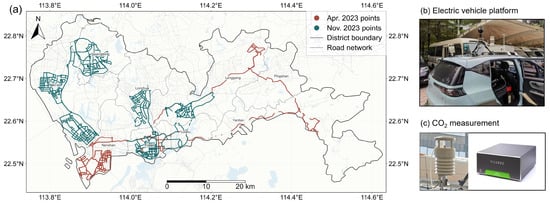
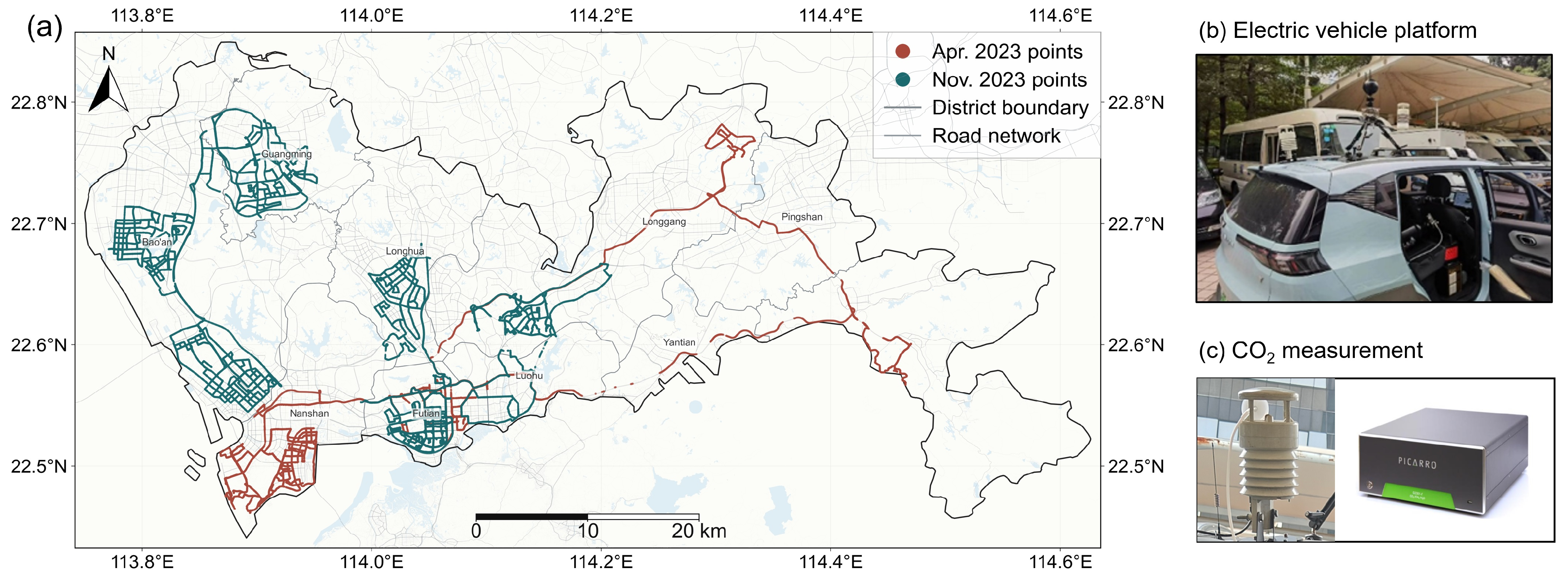
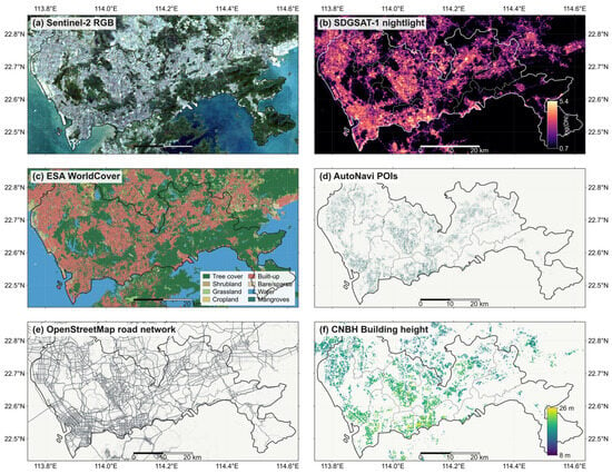
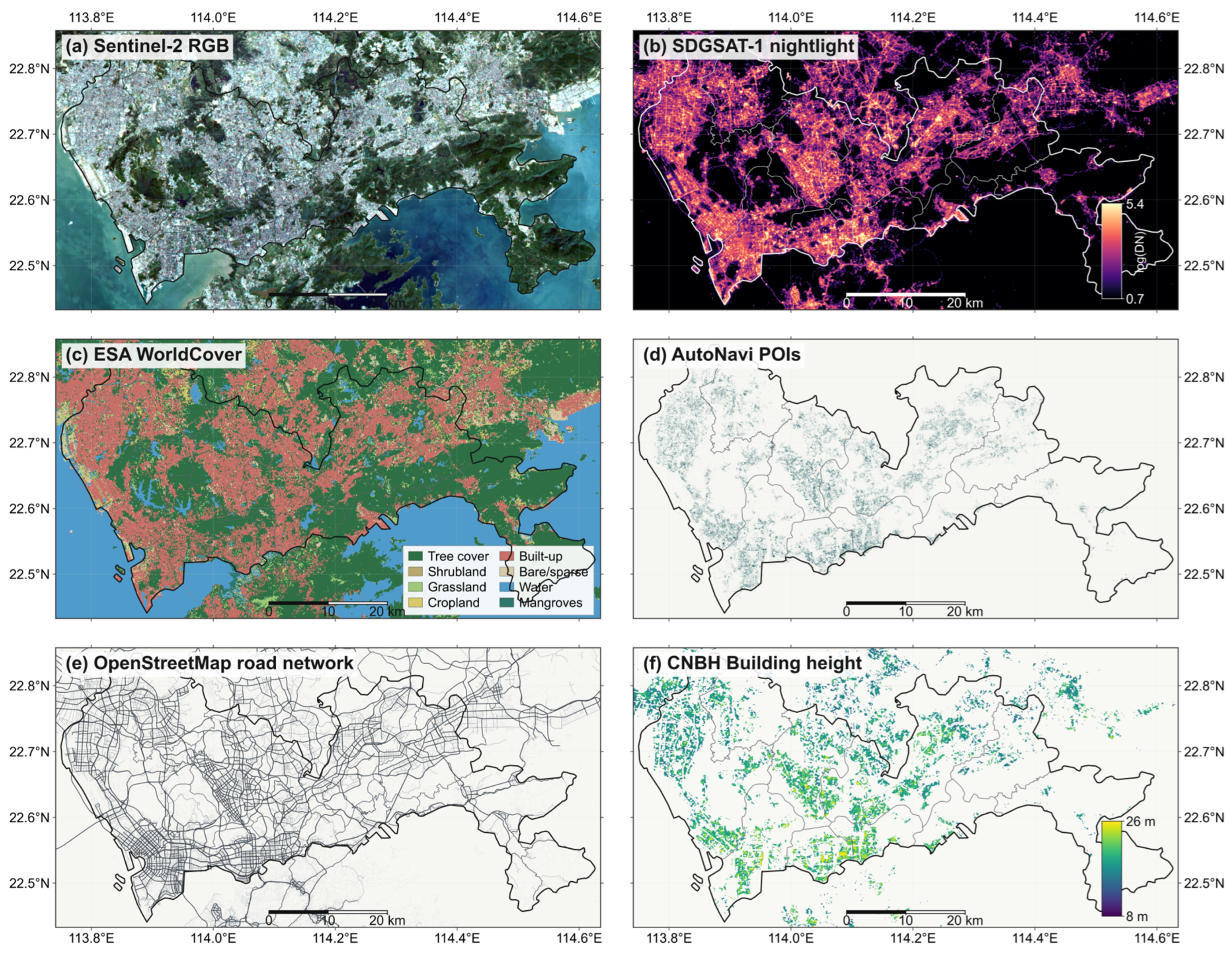
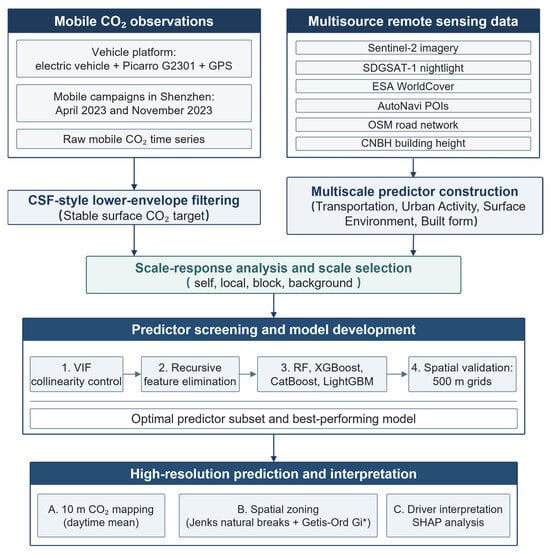
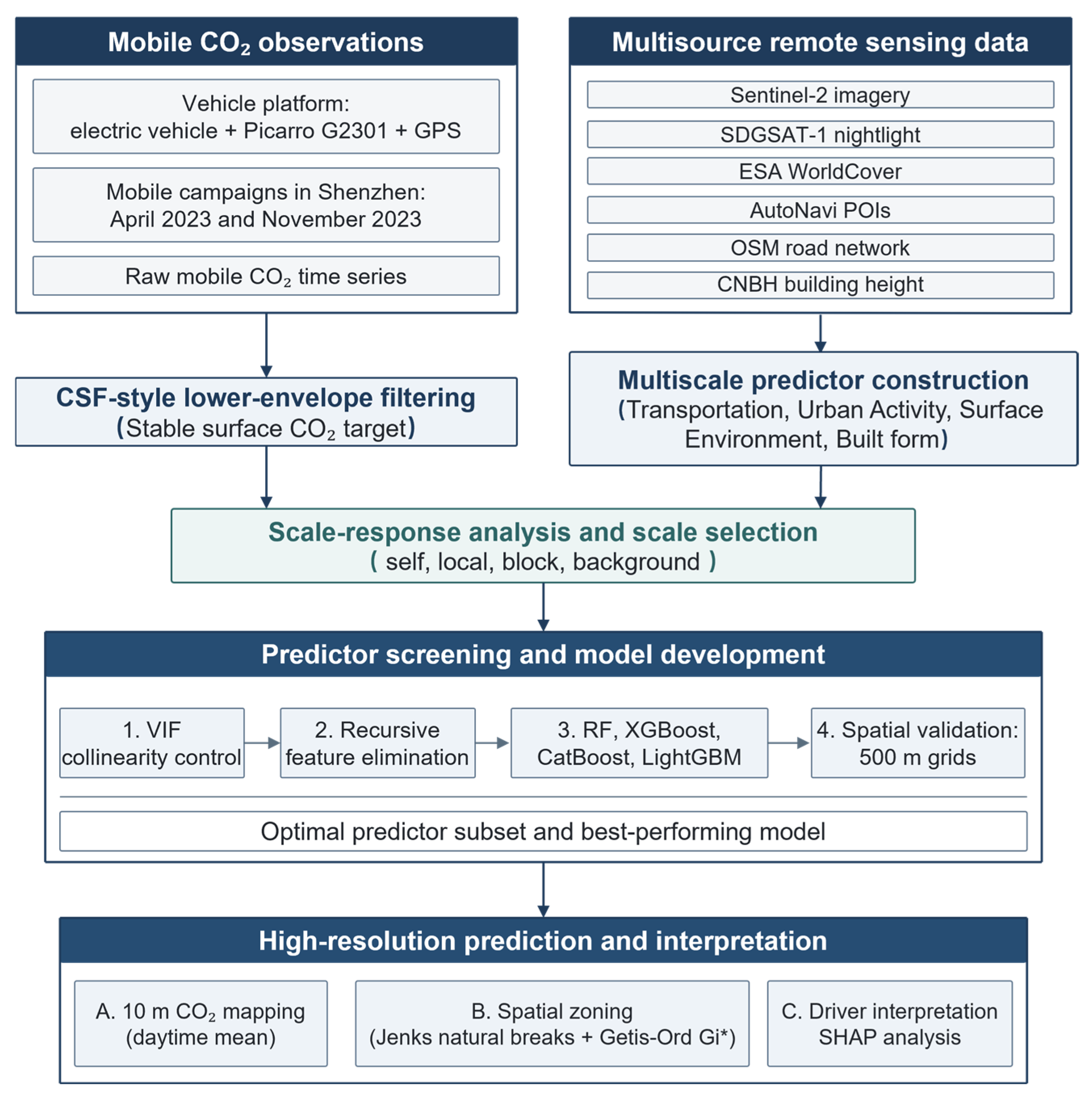
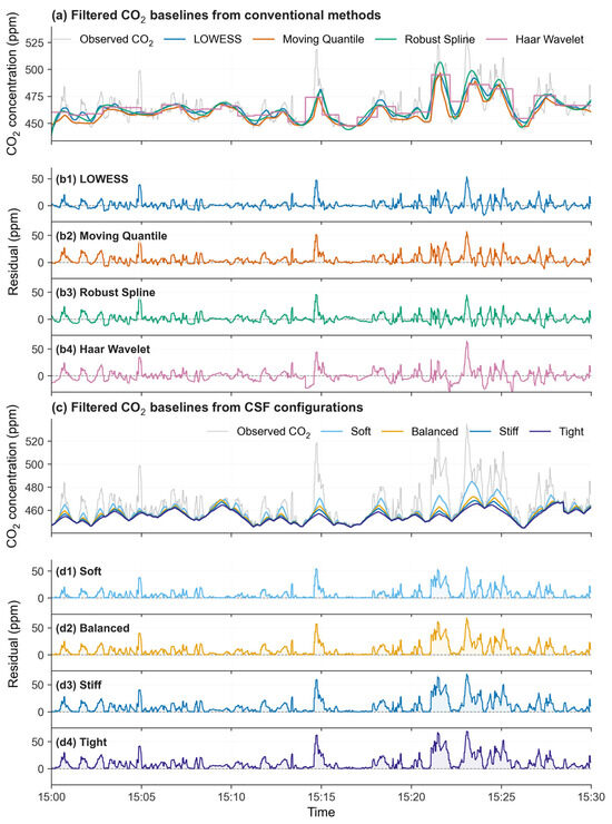
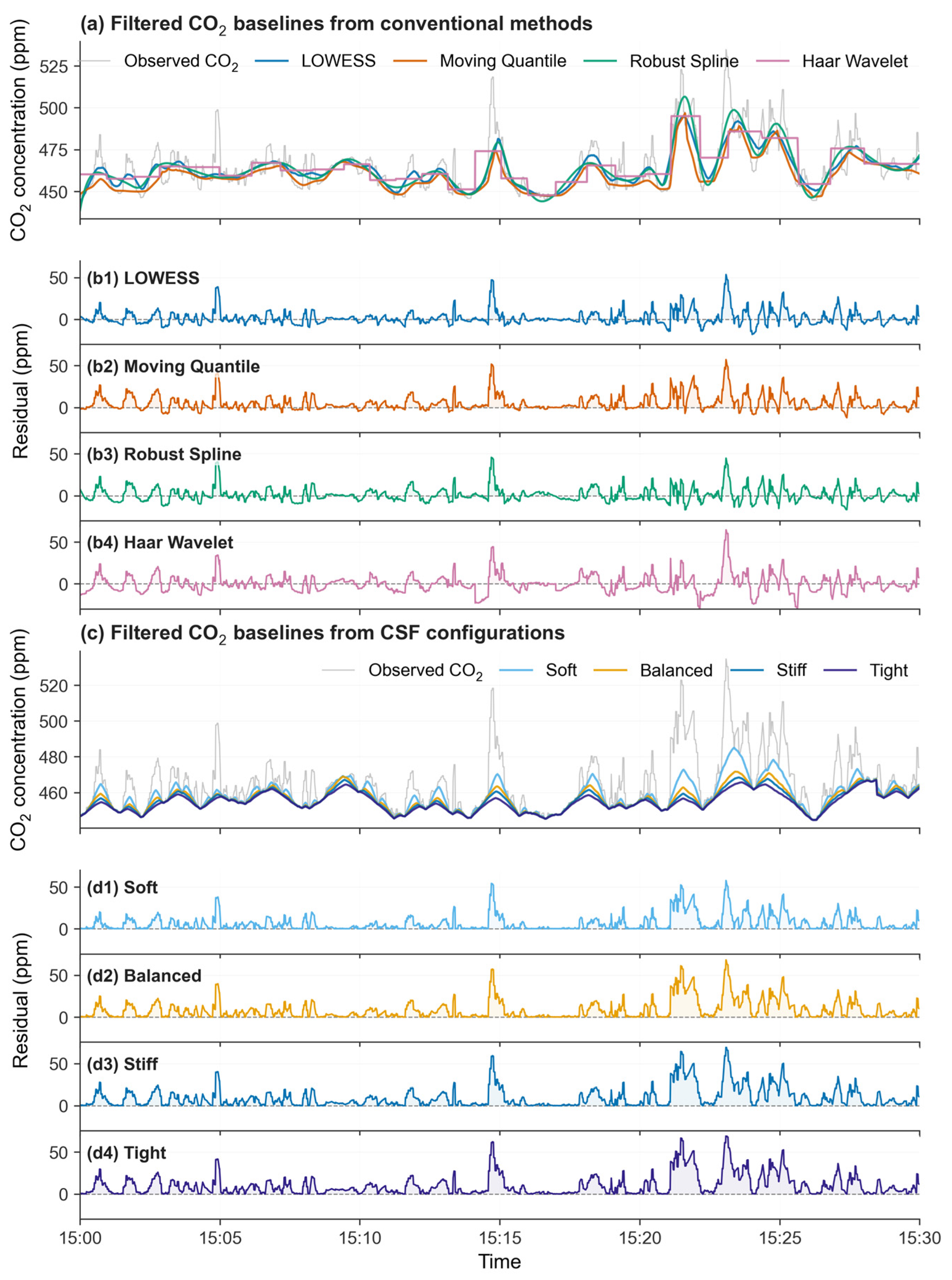
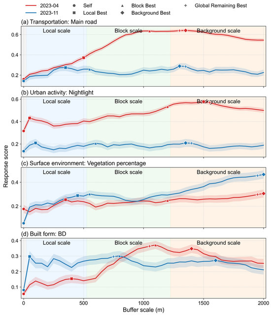
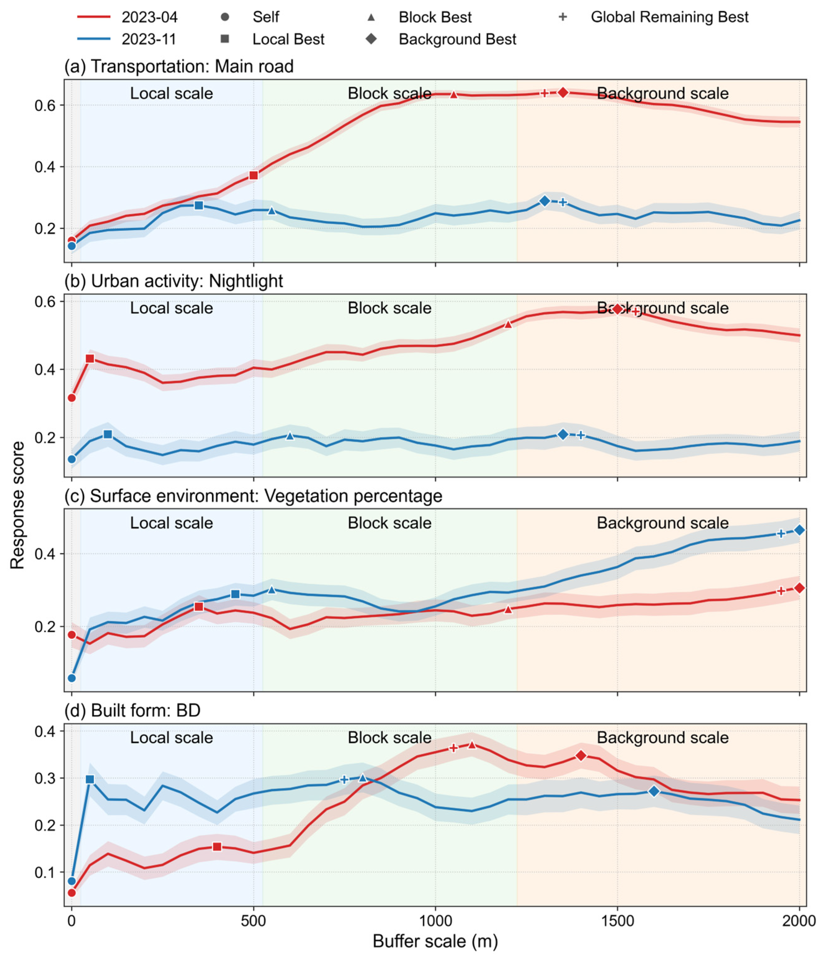
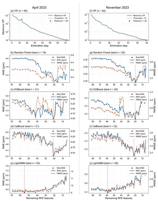
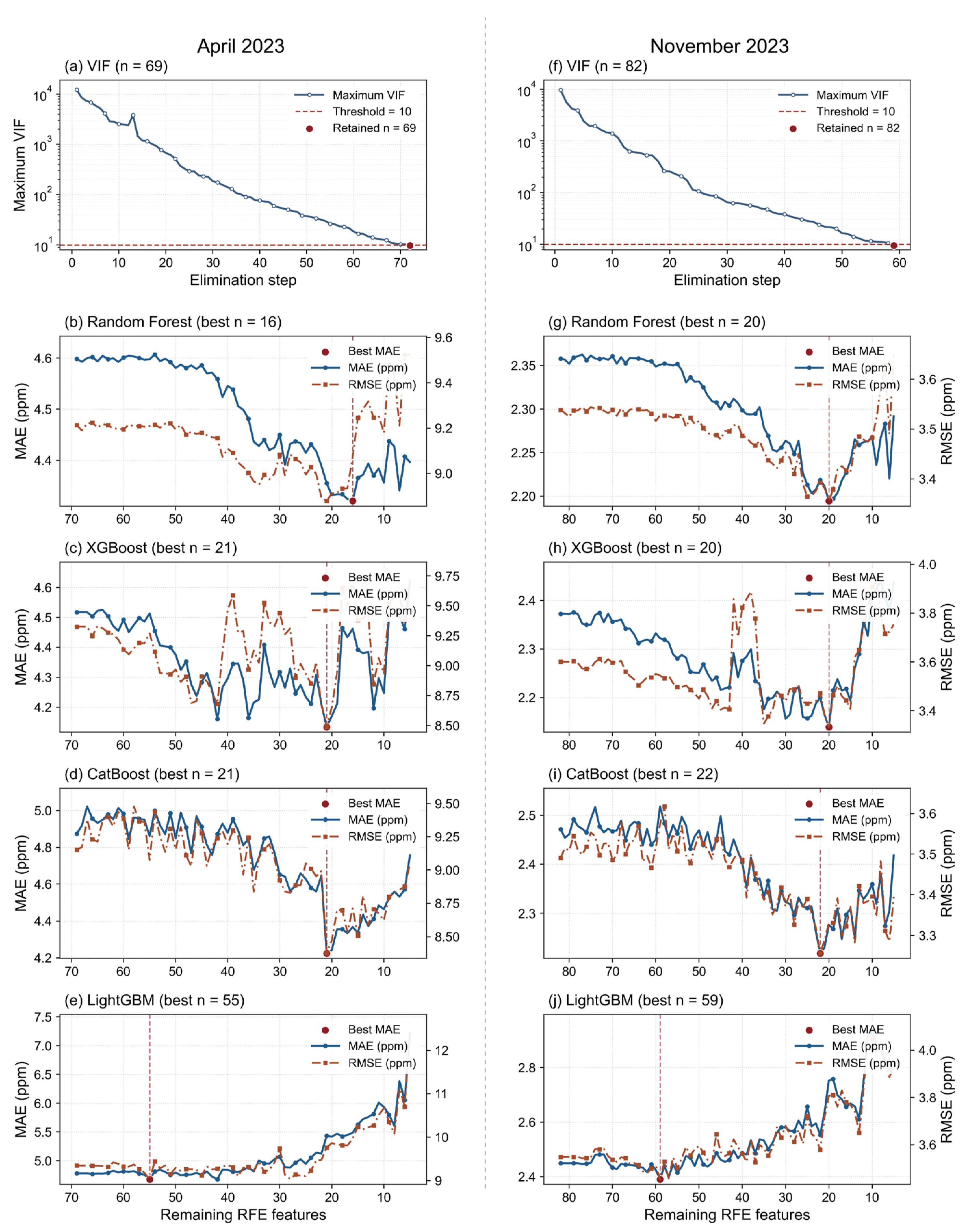
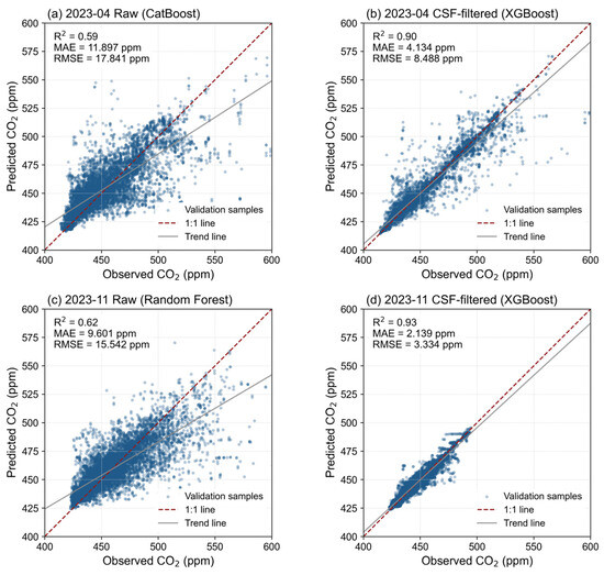
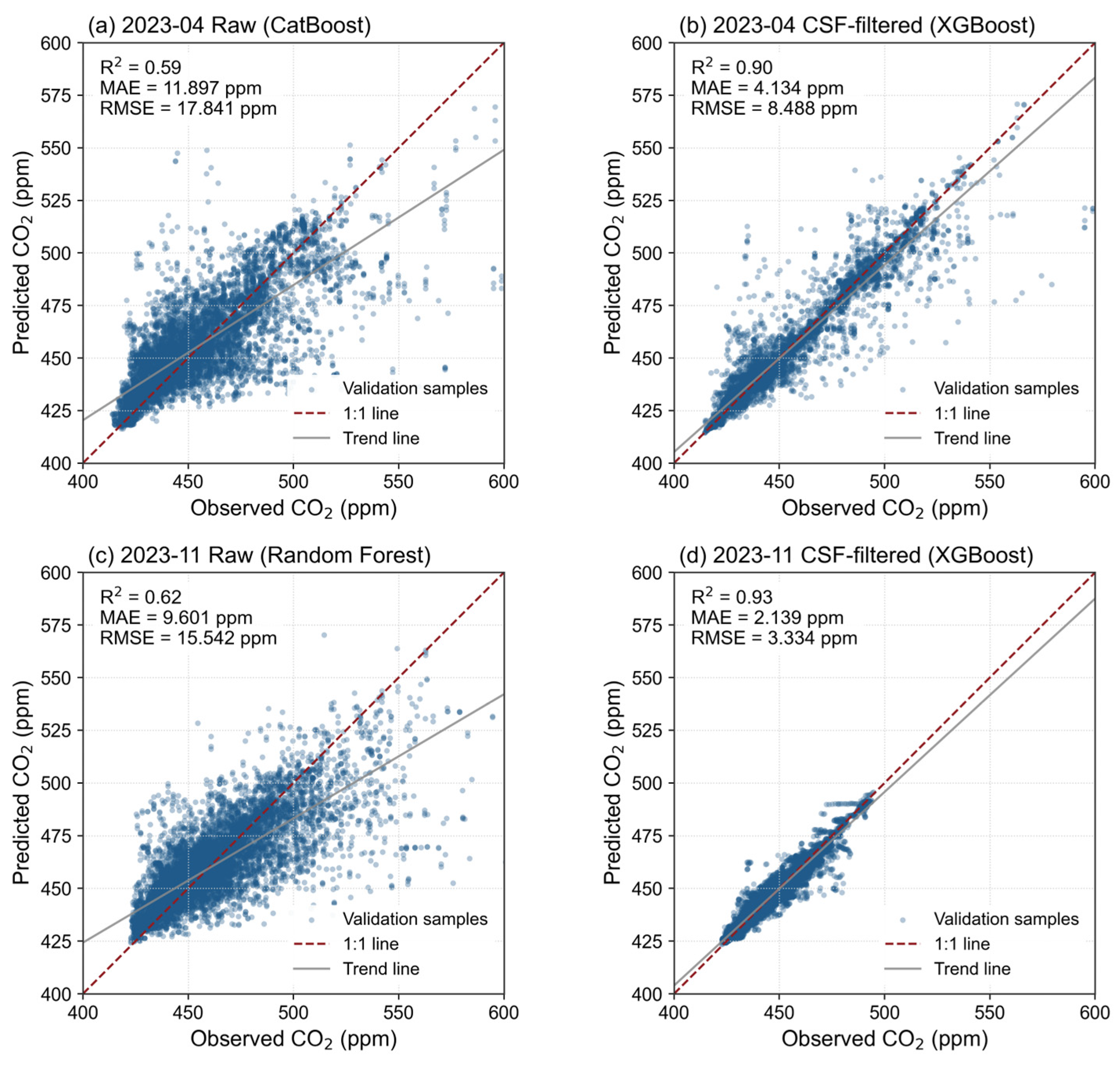
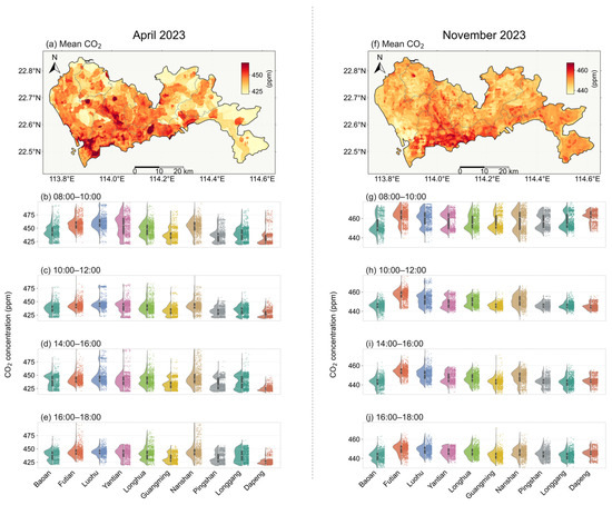
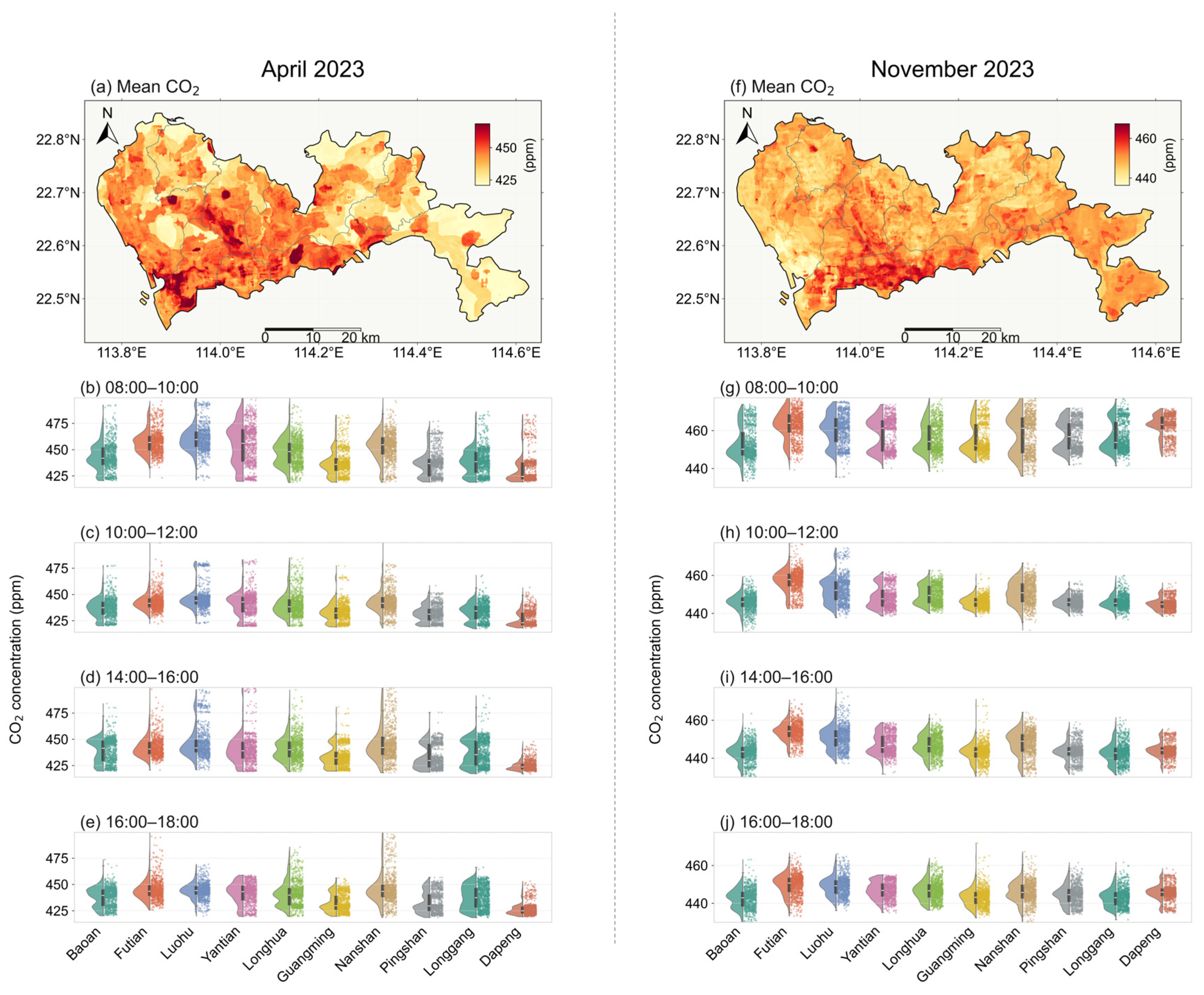
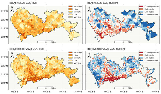
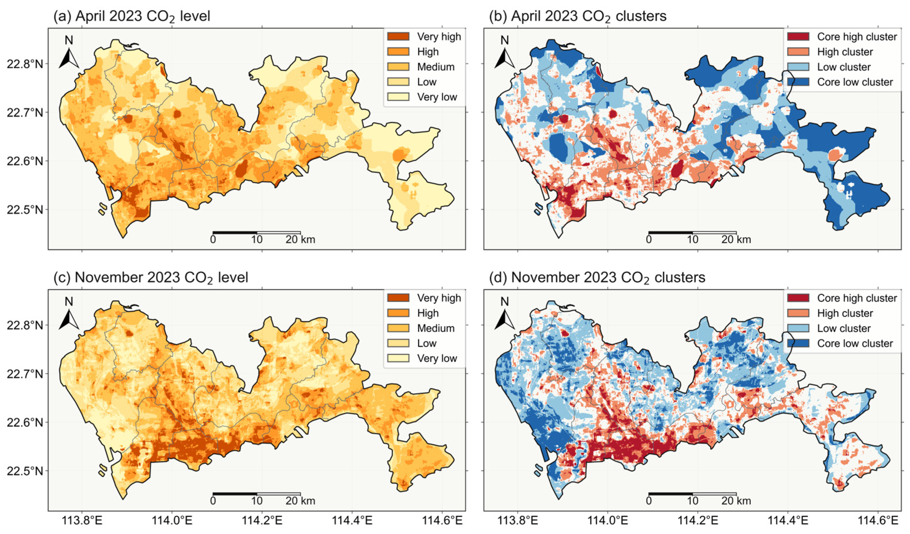
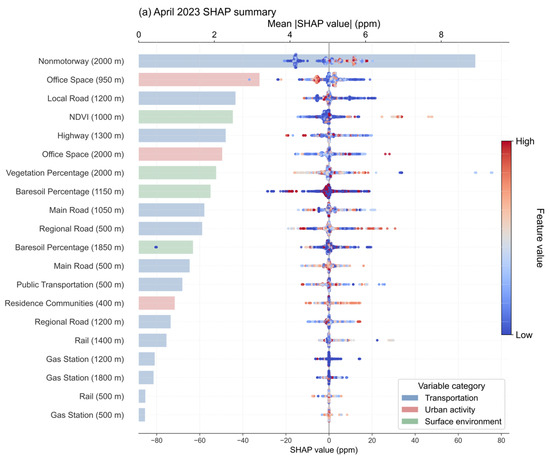
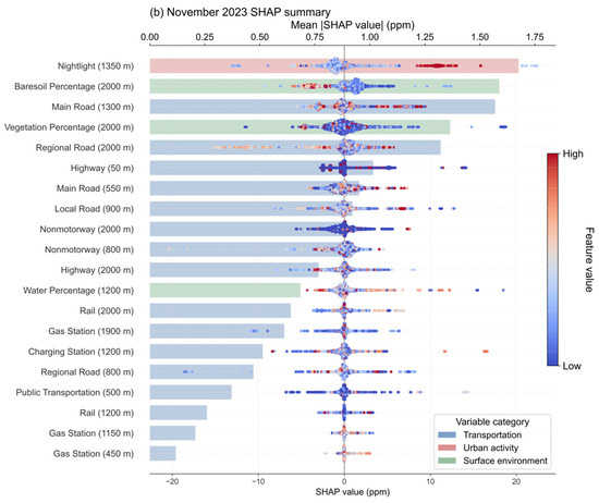
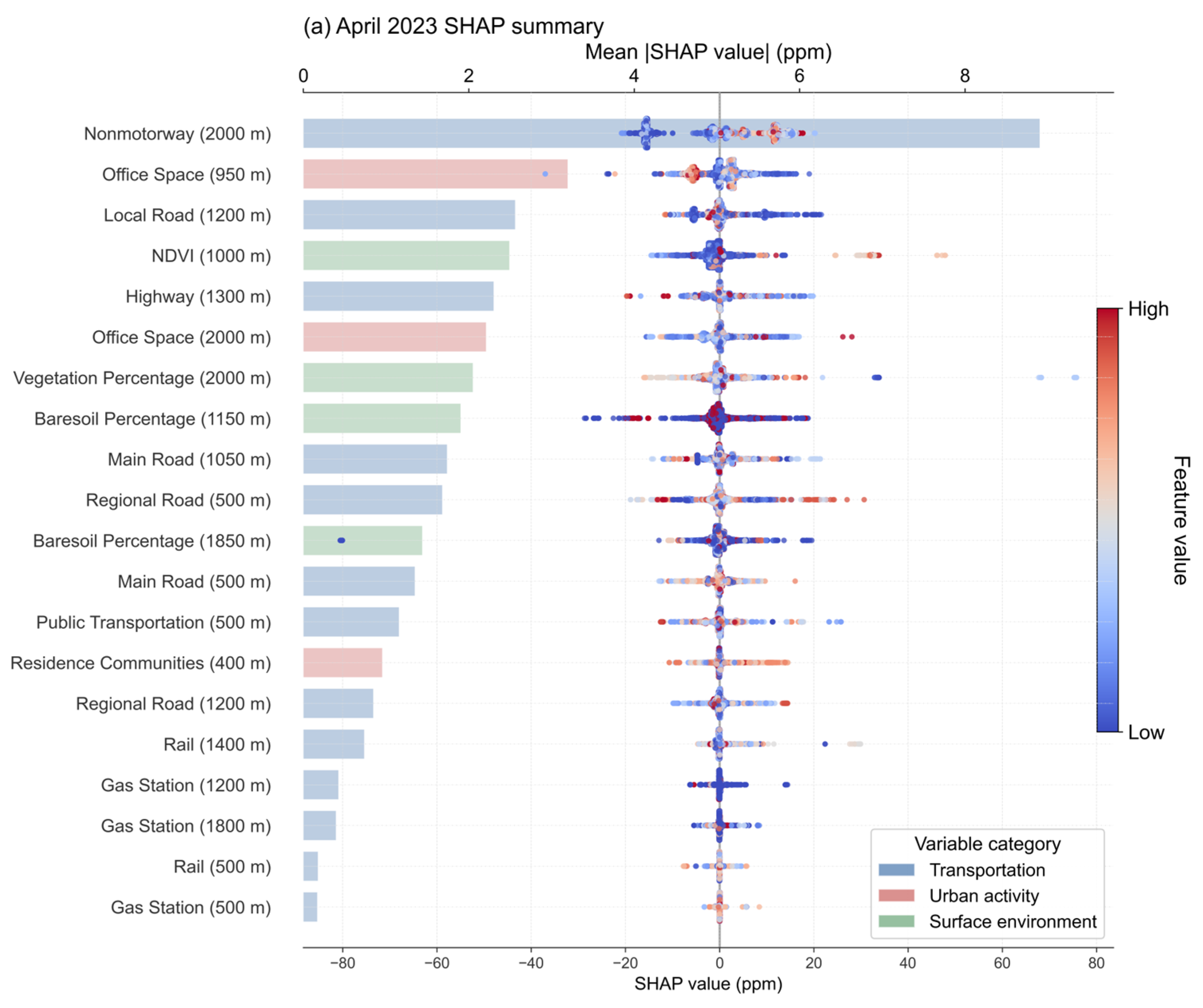
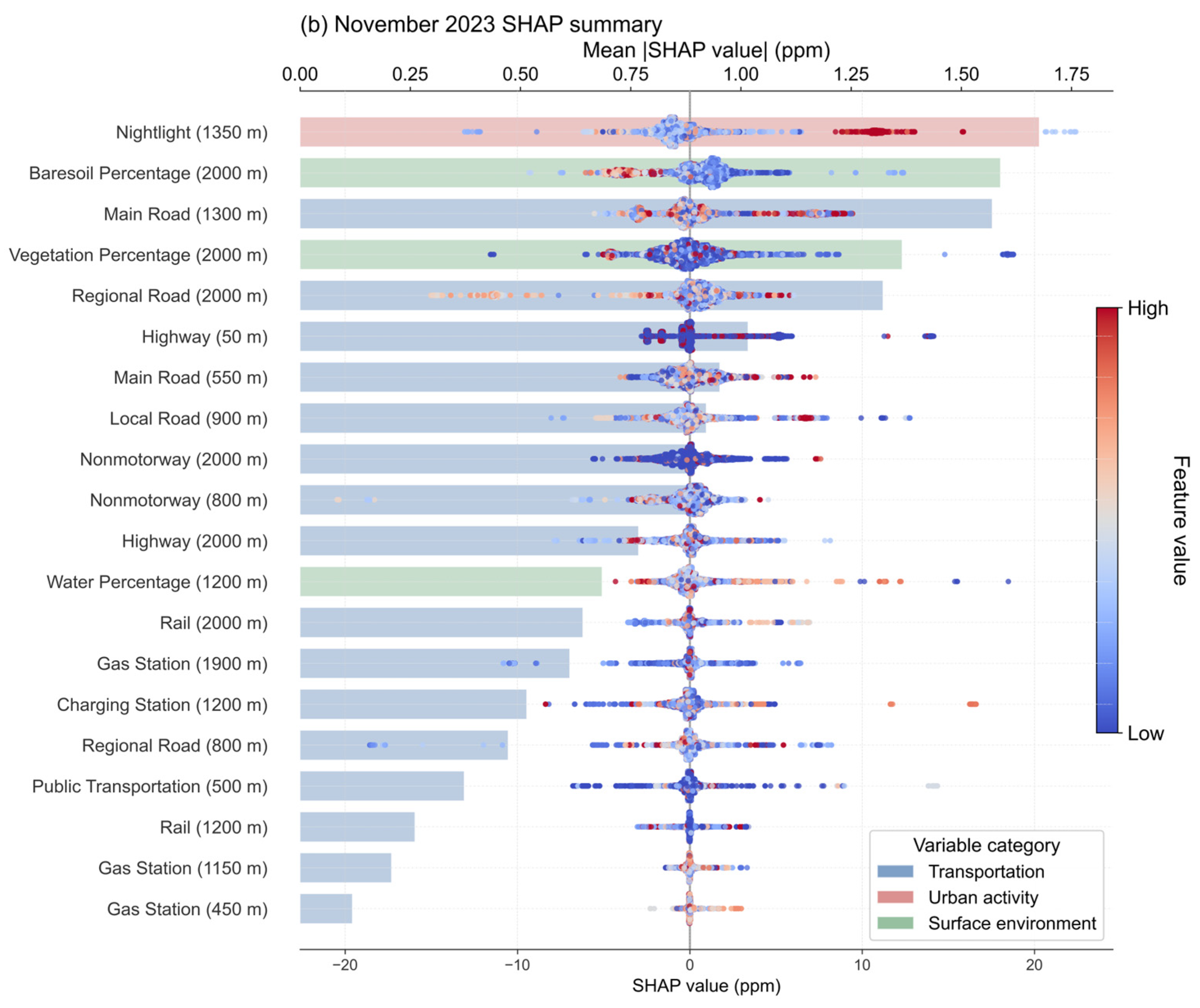

Disclaimer/Publisher’s Note: The statements, opinions and data contained in all publications are solely those of the individual author(s) and contributor(s) and not of MDPI and/or the editor(s). MDPI and/or the editor(s) disclaim responsibility for any injury to people or property resulting from any ideas, methods, instructions or products referred to in the content. |
© 2026 by the authors. Licensee MDPI, Basel, Switzerland. This article is an open access article distributed under the terms and conditions of the Creative Commons Attribution (CC BY) license.