Development and Verification of an Automatic Tower-Based SIF Observation System Based on Narrow Field-of-View Scanning and DOAS Atmospheric Correction

Highlights

What are the main findings?

• The tower-based system retrieves SIF via DOAS in Fraunhofer lines, avoiding O₂-band atmospheric errors and improving cloudy-sky stability.
• H₂O absorption cross-sections are built into the fitting, enabling reliable SIF retrieval in the water-vapour band through active correction.

What are the implications of the main findings?

• This atmospheric robustness enables high-precision tower-based SIF observation under cloudy and humid conditions.
• It supports phenology tracking over a full crop rotation, providing a reliable near-surface benchmark for satellite SIF.

Abstract

Sun-induced chlorophyll fluorescence (SIF) is an effective proxy for vegetation photosynthesis, but tower-based retrieval suffers from atmospheric path interference under humid and variable conditions. We present a DOAS-based SIF retrieval algorithm that operates in Fraunhofer lines (680–686 nm, 745–758 nm) and water vapour-sensitive bands (717–727 nm). It constructs an adaptive reference spectrum from SCOPE simulations and PCA and incorporates H₂O absorption cross-sections into the fitting process for active atmospheric correction. The algorithm is implemented in a dedicated tower-based system integrating a 1° scanning gimbal with a high-resolution spectrometer. Validation with simulated and field data demonstrates the following: (1) the algorithm retrieves SIF with high fidelity (correlation coefficients >0.9 across all windows); (2) it exhibits lower water-vapour sensitivity and greater cloudy-sky stability than FLD, 3FLD, and SFM, achieving the lowest coefficient of variation (CV = 0.356); (3) over a complete wheat–rice rotation, the retrieved SIF tracks crop growth and phenological stages. This work provides a reliable solution for automated, high-precision tower-based SIF observation under complex atmospheric conditions.

1. Introduction

Sun-induced chlorophyll fluorescence (SIF) constitutes the optical signal emitted by chlorophyll a molecules within the 650–850 nm wavelength range, following vegetation’s absorption of photosynthetically active radiation (PAR). As a direct product of the photosynthetic electron transport chain, SIF serves as a robust remote sensing proxy for monitoring both gross primary productivity (GPP) and the physiological state of vegetation.

Under natural illumination conditions, the fluorescence signal is blended within the photosynthetically active radiation, making its isolation challenging. According to the Fraunhofer line principle [1], at absorption lines within the solar or terrestrial atmosphere, differences arise between solar irradiance and vegetation radiance intensity due to the fluorescence filling effect. This discrepancy is amplified at these absorption lines. Under sufficiently high-resolution spectroscopic detection, this filling effect can be identified and quantified through certain assumptions. Currently, the most prevalent method for ground-based SIF observation is the Fraunhofer Line Discriminator (FLD) and its derivatives (e.g., 3FLD, iFLD) [2,3,4]. These methods utilise the radiation difference within and outside Earth’s strong atmospheric absorption bands (typically the oxygen O₂–A band at 760 nm and the O₂–B band at 687 nm) to determine SIF. This approach requires only spectral values within and outside the absorption wavelength, and as the fluorescence signal is relatively strong in these bands, it can be relatively easily decoupled. Consequently, SIF retrieval is achievable even with lower spectral resolution, leading to its widespread adoption across multiple ground-based SIF observation systems. Systems such as FLOX (http://jb-hyperspectral.com), FluoSpec, and SIFSpec, mounted on the ground or towers, can simultaneously measure SIF and reflectance values for vegetation at different heights [5,6]. However, retrieval methods within atmospheric absorption bands rely on the assumption that fluorescence and reflectance remain constant both inside and outside the absorption lines. In reality, fluorescence and reflectance continuously vary with wavelength. Within atmospheric absorption bands, they are susceptible to interference from atmospheric scattering (e.g., clouds, aerosols) and gas absorption filling effects. Consequently, this method yields suboptimal retrieval results under cloudy conditions [7]. Furthermore, traditional retrieval typically assumes the sensor is positioned at the top of the canopy (TOC), neglecting the atmospheric path between the sensor and the target. However, as sensor altitude increases or solar/observation zenith angles rise, for instance, when the observation platform is a tall tower—even atmospheric paths of a few metres can induce significant SIF retrieval errors [8]. Sabater et al. quantified the error propagation and impact of neglecting oxygen absorption effects through simulations and field measurements, proposing an improved compensation strategy for O₂-A absorption band measurements [9].

To circumvent the atmospheric scattering and path-length issues inherent in oxygen-band methods, solar Fraunhofer lines—which originate above Earth’s atmosphere—offer an alternative retrieval pathway. Originating from the Sun’s photosphere, these lines are theoretically more stable as they remain unaffected by Earth’s atmosphere [10]. Fraunhofer line methods are predominantly employed for satellite-based SIF data retrieval to circumvent the interference of long atmospheric paths. For instance, Köhler et al. utilised linear methods for SIF retrieval in the 720–758 nm band for GOME-2 and SCIAMACHY satellites [11]. For ground-based platforms, Guanter et al. employed the SVD method to achieve retrievals in the oxygen, water vapour, and Fraunhofer line bands [12]. However, this statistical approach relies heavily on extensive data, being based on statistical or phenomenological characteristics derived from the data. Consequently, the physical significance of the retrieved parameters (such as singular vector weights or relative optical paths) is not immediately apparent. Grossmann et al. developed the PhotoSpec system [10], employing narrow-field scanning and methods grounded in DOAS (differential optical absorption spectroscopy) theory to retrieve SIF by fitting the Fraunhofer lines. This represents an entirely novel ground-based SIF observation system. Crucially, however, their retrieval scheme deliberately avoids the strong water vapour absorption bands, leaving a critical gap for tower-based observations in humid environments.

Compared with SIF signals obtained at a few absorption lines, multi-band or full SIF spectra can provide more information; for example, SIF ratios in the far-red and red regions can indicate whether vegetation is suffering from stressors such as low temperatures or drought [13], and some studies have also shown that they are proportional to light use efficiency [14]. Consequently, researchers have explored the construction of SIF across the full spectral range; Zhao et al. developed the AFSR method, which utilises linear combinations of fundamental spectra to fit SIF spectra and reflectance curves [15]. Naethe et al. further developed a machine learning-based partial least squares (PLS) regression algorithm, which, by exploiting the covariance structure between spectral derivatives and SIF, achieves a processing speed 37 times faster than that of conventional fitting methods, and supports both sub-band and full-band retrieval [16]. However, both the AFSR and PLS methods are inherently data-driven, requiring extensive training data that limit their generalizability across diverse vegetation types and atmospheric conditions. Furthermore, the PLS retrieval, like other statistical approaches, offers limited physical interpretability, and its full-spectrum application deliberately excludes the O₂–A and O₂–B absorption bands.

The rationale for the present approach follows directly from the two gaps identified above. On the one hand, the PhotoSpec system demonstrates that a physically interpretable, DOAS-based retrieval within Fraunhofer lines is feasible for tower-based observations, but its deliberate avoidance of the water vapour absorption band leaves humid environments unaddressed; on the other hand, the AFSR and PLS methods extend SIF retrieval across the full spectrum but do so through data-driven fitting, which limits both their physical interpretability and their generalisability across vegetation types and atmospheric conditions. Building on the physically grounded DOAS framework while avoiding a purely data-driven construction of the reference spectrum, this study therefore combines a model-based reference SIF spectrum with explicit, physically interpretable water vapour correction, so as to close both gaps simultaneously. Specifically, this study proposes a model-driven DOAS retrieval framework with two key innovations: (1) an adaptive reference SIF spectrum constructed from SCOPE simulations combined with PCA, avoiding empirically averaged spectra; (2) explicit inclusion of H₂O absorption cross-sections in the fitting equation for active gas correction. We further construct a forward model of H₂O absorption along the 20 m tower-to-canopy path using HITRAN cross-sections and the Beer–Lambert law, and evaluate retrieval errors under varying temperature, humidity, and path-length scenarios. The method is implemented in a tower-based system integrating a narrow-field-of-view (1°) scanning gimbal with a high-resolution spectrometer, and validated through simulations and long-term field measurements over a wheat–rice rotation.

2. Materials and Methods

2.1. SIF Retrieval Method

2.1.1. SIF Retrieval Method Based on DOAS

The commonly employed SIF retrieval methods for ground/tower-based systems are the FLD method and its derivative techniques. This approach fundamentally assumes that fluorescence and reflectance remain constant both inside and outside the absorption dark line. However, Sabater et al. quantified the impact of oxygen transmittance correction on SIF retrieval within oxygen absorption bands, demonstrating that atmospheric effects cannot be disregarded [8]. To overcome this assumption, our approach focuses on the solar Fraunhofer lines, while also explicitly incorporating the water vapor-sensitive band through active atmospheric correction. Based on DOAS theory—a common technique in trace gas monitoring—it separates the effects of reflectance, gases, and SIF signals at atmospheric absorption lines by dividing spectral variations into narrowband and broadband components [17]. First, without considering atmospheric effects, the incident and outgoing light from vegetation can be expressed respectively as:

$$E=E_0·T_{\uparrow }$$

(1)

$$L={\displaystyle \frac{E_0}{\pi }}·R_{\downarrow }+SIF$$

(2)

where $T_{\uparrow }$ denotes the reflectivity/transmissivity of the upward-facing reference diffuser (cosine corrector), while $R_{\downarrow }$ denotes the canopy reflectance. E₀ signifies the incident solar irradiance, with E and L denoting the absolutely radiometrically calibrated spectral intensities received by the upward- and downward-facing channels, respectively (Section 2.3). In Equation (2), the factor π converts the incident solar irradiance E₀ into an equivalent radiance under the Lambertian assumption, consistent with the canopy radiance L. Atmospheric transmission along the sensor–canopy path is not considered at this stage; it is introduced explicitly through the gas absorption term in Equation (4). We further note that E and L are, strictly, different radiometric quantities (irradiance and radiance, respectively) and are therefore not expressed in identical units; however, because this unit/geometric scale factor is wavelength-independent across the narrow retrieval window, it is absorbed into the low-order broadband polynomial term in Equation (4) during the least-squares fit and does not bias the retrieved narrowband SIF or gas absorption structure. Expressing spectral variations in terms of optical density and employing a logarithmic Taylor series approximation yields the following Equation:

$$ln\left({\displaystyle \frac{L}{E}}\right)=ln\left({\displaystyle \frac{R_{\downarrow }}{{\pi T}_{\uparrow }}}\right)+ln\left(1+{\displaystyle \frac{\pi SIF}{E_0{R}_{\downarrow }}}\right)\approx ln\left({\displaystyle \frac{R_{\downarrow }}{{\pi T}_{\uparrow }}}\right)+{\displaystyle \frac{SIF}{L}}$$

(3)

The approximation in Equation (3) employs a first-order Taylor expansion of the logarithmic term, ln (1 + $\pi$SIF/$E_0{R}_{\downarrow }$) ≈ SIF/L, which holds when SIF constitutes a small fraction of the total upwelling radiance (SIF/L ≪ 1). This condition is generally satisfied in the far-red region, where SIF typically accounts for only a few percent of the canopy radiance. As SIF increases relative to L, the higher-order residual of the expansion introduces a small negative bias, the implications of which are examined in Section 4. Spectral variations are categorised into narrowband and broadband shifts. Broadband effects arising from transmittance and reflectance are modelled using polynomial terms $P_k\left(j\right)$. The shape and magnitude of the SIF are expressed as the product of the reference spectrum $R_{SIF}$ and the fitting factor $S_{SIF}$. Unlike space-based retrieval of SIF signals, tower-based observations may focus solely on the distance between the sensor and the target. Atmospheric effects are incorporated into the equation as gas absorption cross-sections ${\sigma }_i$, and the fitting factors can be calculated using a least-squares fitting method, as shown in Equation (4):

$${\Vert ln\left({\displaystyle \frac{L\left(\lambda \right)}{E\left(\lambda \right)}}\right)-P_k\left(\lambda \right)-{\displaystyle \frac{R_{SIF}\left(\lambda \right)}{L\left(\lambda \right)}}{S}_{SIF}-\sum {\sigma }_i{S}_i\left(\lambda \right)\Vert }^2\to min$$

(4)

L and E denote the solar irradiance and vegetation radiance measured by the spectroradiometer, respectively. These values are obtained for each measurement combination following dark current correction and radiometric calibration (see Section 2.3). Vegetation surface reflectance and sensor transmittance are fitted using low-order polynomials at each wavelength. The experimental tests in this study revealed that the fourth-order Legendre polynomial (k = 4) provided the best-fit result.

For comparison with the DOAS retrieval, SIF was also retrieved using FLD, 3FLD, and the Spectral Fitting Method (SFM). FLD used reference/absorption band pairs at 758/760 nm (far-red) and 685/686 nm (red); 3FLD added a second reference band (766 nm and 689 nm, respectively), combined via distance-weighted interpolation. SFM fitted reflectance and SIF as linear functions of wavelength via least-squares regression over the windows 758–767.6 nm (far-red) and 685–691 nm (red).

2.1.2. Construction of Reference SIF Spectroscopy ($R_{SIF}$)

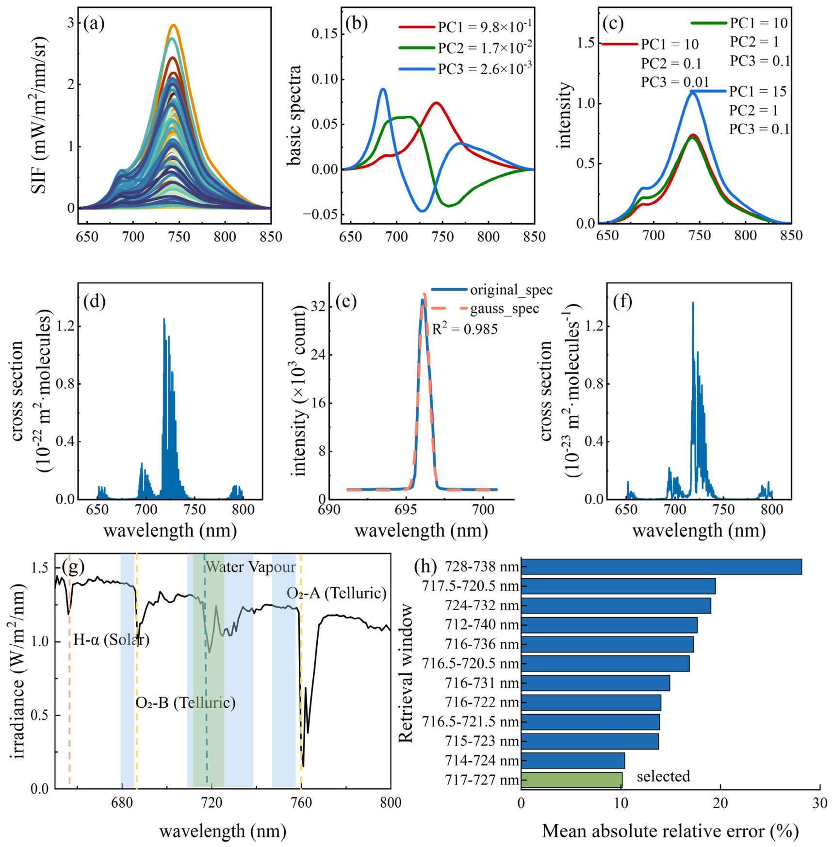
$R_{SIF}$ is a key parameter for SIF retrieval. The reference SIF spectrum, $R_{SIF}$, is generated with the SCOPE (Soil Canopy Observation, Photochemistry and Energy fluxes) model, which is a canopy radiative transfer model incorporating fluorescence emission [18]. This model categorises factors influencing canopy radiative transfer processes into distinct types, including leaf biochemistry, soil, canopy structure, microclimate, and observation angle parameters. By altering parameter ranges, the emission light, reflected light, and fluorescence spectra of vegetation are simulated with different species and growth conditions. Following discussions by Verrelst et al. [19], the most influential model parameters affecting fluorescence signal emission were selected. These parameters are assigned random values within a reasonable range. All parameter settings are detailed in

Table A1. The input parameters and the settings of the SCOPE model.

Parameters	Interpretation	Range	Unit
Cab	Chlorophyll content	5–80 *	mg/cm2
Cdm	Dry matter content	0–0.05	g/cm2
Cs	Senescence factor	0–0.9	--
LAI	Leaf area index	0–7	m2/m2
LIDFa	Leaf Inclination Distribution Function (LIDF) parameter a	−1–1	--
Vcmo	Maximum carboxylation capacity	0–200	μmol/m2/s
hc	Canopy height	0.1–2	m
lw	Leaf width	0.01–0.1	m
spectrum	Soil spectrum	--	--
Rin	Incoming shortwave radiation	0–1400	W/m2

* The lower bound of Cab was set to 5 mg/cm² to exclude senescent or dead vegetation scenarios that are not relevant to our tower-based observations over healthy wheat and rice canopies.

. The relative heights of the two fluorescence peaks are primarily regulated by Cab. Beyond considering leaf and canopy attributes intrinsic to the vegetation, assumptions were made regarding the soil background spectrum and microclimatic conditions. It was also assumed that the observation angle remained constant based on ground-level measurements. The selected parameters were sampled within their respective ranges using Latin hypercube sampling (LHS), which provides a more uniform and space-filling coverage of the multi-dimensional parameter space than simple Monte Carlo sampling; a fixed random seed was used to ensure reproducibility. In this way, a total of 1000 independent fluorescence spectra were generated as reference spectra, a representative subset of which is shown in Figure 1a. Before feature extraction, each spectrum was standardised across wavelengths using min–max scaling, so that all wavelength bands contributed comparably to the subsequent analysis rather than being dominated by high-amplitude bands. The PCA method was used to extract features from these reference spectra, yielding the first three principal components, as shown in Figure 1b. It can be seen that the fluorescence structure is primarily governed by the first three principal components, which together account for 99.99% of the variance. Different combinations of coefficients can simulate SIF curves under various conditions, as shown in Figure 1c. By randomly assigning different coefficients to the three principal components, it can be observed that there are differences in both their intensity and structure. Because the three principal components are extracted from the same 1000 SCOPE-simulated spectra that constitute the reference library, evaluating reconstruction accuracy on this same set alone would yield an optimistic, in-sample estimate that does not establish whether the components generalise to spectra outside this set. To evaluate the generalisability of the extracted principal components, we performed a 10-fold cross-validation on the 1000 simulated spectra. The reason for choosing 10-fold cross-validation instead of other types of cross-validation is that for stable linear methods such as PCA that are applied to this sample size, 10-fold cross-validation significantly reduces the computational requirements when achieving similar results [20]. The reconstruction error for the validation set remained below 0.58%, confirming that the first three PCs provide a stable and representative basis for describing SIF spectral variability across different vegetation conditions.

According to Verhoef et al., PC1 primarily represents the average intensity and basic profile of the fluorescence spectrum, while PC2 and PC3 mainly capture changes in the ratio of the red (685 nm) and far-red (740 nm) peaks caused by chlorophyll reabsorption effects, as well as shifts in the spectral fine structure [21]. Therefore, to enhance the generalisability of the SIF retrieval algorithm across different physiological states of vegetation, this study abandoned the traditional assumption of a single fixed fluorescence shape and constructed an adaptive reference spectral model based on a combination of multiple principal components (in this study, a combination of the first three principal components was adopted), enabling the retrieval system to adaptively adjust the reference fluorescence shape according to the measured spectra. By modifying the SIF fitting term in Equation (4), the updated retrieval objective function is:

$${\Vert ln\left({\displaystyle \frac{L\left(\lambda \right)}{E\left(\lambda \right)}}\right)-P_k\left(\lambda \right)-{\displaystyle \frac{{\sum }_{j=1}^3{\alpha }_j\cdot P{C}_j\left(\lambda \right)}{L\left(\lambda \right)}}-\sum {\sigma }_i{S}_i\left(\lambda \right)\Vert }^2\to min$$

(5)

where $P{C}_j\left(\lambda \right)$ represents the first three principal component vectors extracted via PCA, while ${\alpha }_j$ denotes the fitting coefficient corresponding to the j-th principal component. This improvement enables the algorithm not only to estimate the intensity of the SIF when dealing with different species or stressed vegetation, but also to detect subtle dynamic shifts in the spectral characteristics of the vegetation through changes in the coefficients.

2.1.3. Atmospheric Gas Correction

High-resolution gas absorption cross-sections ${\sigma }_i$ are sourced from HITRAN (the High-Resolution Transmission molecular absorption database). This database contains spectral absorption line data for numerous molecules under diverse environmental conditions, primarily serving to simulate and analyse the spectral characteristics of atmospheric gas molecules. It supports applications spanning the ultraviolet to infrared wavelength range [22]. Figure 1d shows the high-resolution water vapour absorption cross-section within the range of 650–800 nm. The high-resolution gas absorption cross-section needs to be convolved with the instrument function before being used to ensure that the spectral absorption cross-section distribution matches the instrument wavelength. The mercury lamp peak measured by the instrument at around 696 nm was fitted with a Gaussian function to obtain the instrument function of the spectrometer, as shown in Figure 1e. Figure 1f presents a schematic diagram of the high-resolution water vapour absorption cross-section and the absorption cross-section after convolution with the instrument function. Here, the absorption cross-section is convolved with an FWHM of 0.3 nm, which is consistent with the spectral resolution capability of the QE Pro spectrometer (OceanOptics Inc., Dunedin, FL, USA) used in the actual observation system, to ensure that this cross-section is suitable for the retrieval process of this study.

2.2. Water Vapour Influence on Simulation and Band Selection

To investigate the effect of varying water vapour concentrations on the retrieval method, this study also developed a forward model of water vapour absorption along the transmission path from the tower base to the sensor. First, the partial pressure of water vapour in the air was calculated using the Magnus equation based on temperature T (°C) and relative humidity RH (%), yielding $e$ in hPa; this value was converted to SI units (Pa) before being used to determine the number density of water vapour via the ideal gas law:

$$e=RH·6.112·exp\left(17.62·T/\left(243.12+T\right)\right)$$

(6)

$$n_{H_{2}O}=e/\left(k_B·T_K\right)$$

(7)

where $k_B$ is the Boltzmann constant (1.380649 × 10⁻²³ J·K⁻¹), and $T_K$ (K) = T + 273.15. Multiplying this by the path length $L_{path}$ (m) from the sensor to the canopy (default 20 m, maximum 30 m) yields the column density $N$ (molecules·cm⁻²), and the path transmittance is calculated using Beer–Lambert’s law:

$$N=n_{H_{2}O}·L_{path}$$

(8)

$$T_{path}\left(\lambda \right)=exp\left(-{\sigma }_{H_{2}O}\left(\lambda \right)·N\right)$$

(9)

where ${\sigma }_{H_{2}O}\left(\lambda \right)$ (cm²·molecule⁻¹) is the water vapour absorption cross-section at 0.3 nm resolution as provided in the HITRAN database. Finally, the canopy spectrum $L_{canopy}$ is multiplied by $T_{path}$ to obtain the ‘polluted spectrum’ $L_{tower}$ received by the sensor. To cover typical tower-based scenarios, we designed six sets of temperature-relative humidity (RH)/path combinations. Because the primary objective was to generate a range of atmospheric water vapour concentrations, relative humidity was varied as the principal factor, while temperature and path length—both of which also affect the resulting water vapour column density—were varied as secondary factors. The resulting artificial gradients span the dry, moderate, humid, and saturated humidity levels, together with a high-temperature and a long-path scenario, which are typically encountered in near-surface tower-based observations. These combinations correspond to column densities ranging from 3.46 × 10²⁰ to 1.21 × 10²¹ molecules·cm⁻², with the minimum transmittance near the strongest absorption band decreasing to 0.984. The defined combinations are as follows: (1) dry: 20 °C, 30% RH, 20 m; (2) moderate: 20 °C, 50% RH, 20 m; (3) humid: 20 °C, 70% RH, 20 m; (4) wet: 20 °C, 90% RH, 20 m; (5) hot: 30 °C, 60% RH, 20 m; (6) tall_tower: 20 °C, 50% RH, 30 m.

The selection of retrieval windows was designed to test the algorithm’s robustness against atmospheric gas interference under contrasting conditions. The red (680–686 nm) and far-red (745–758 nm) Fraunhofer-line windows, located near the two SIF emission peaks, lie in spectral regions with weak gas absorption and thus serve as ‘clean’ reference windows where atmospheric interference is minimal. In contrast, the water vapour window near 719 nm has strong water vapour absorption and is used as a deliberate “stress test” window to evaluate whether the gas correction scheme can restore accurate SIF under significant atmospheric attenuation conditions. This contrastive design enables us not only to directly assess the fundamental accuracy of the algorithm but also to evaluate its correction capability. Figure 1g shows the reference solar irradiance spectrum derived from the reference atmosphere mass 1.5 (AM1.5G) spectrum in the range of 650 to 800 nm, and also indicates some solar and terrestrial Fraunhofer lines [23], where the pink shaded areas represent the retrieval bands selected in this study.

Specifically, for the water vapour-sensitive window, we further conducted a retrieval window scanning experiment. By setting different combinations of scanning windows with different widths and centre positions, the window that could retain sufficient SIF structural information while minimising the collinearity between the polynomial broadband term and gas absorption was selected as the optimal retrieval window. The candidate windows cover different centre positions and widths within the range of 712–740 nm, including 3–10 nm narrow windows, 15–20 nm wide windows, and a complete 28 nm window. The specific window settings and results are shown in Figure 1h. The results indicate that the 10 nm window in the range of 717–727 nm has the lowest comprehensive error in all water vapour scenarios, and the average relative error across scenarios is approximately 10.15%. Therefore, for the subsequent retrieval of water vapour-sensitive scenarios, 717–727 nm is adopted as the optimal retrieval window.

2.3. Tower-Based SIF Observation System

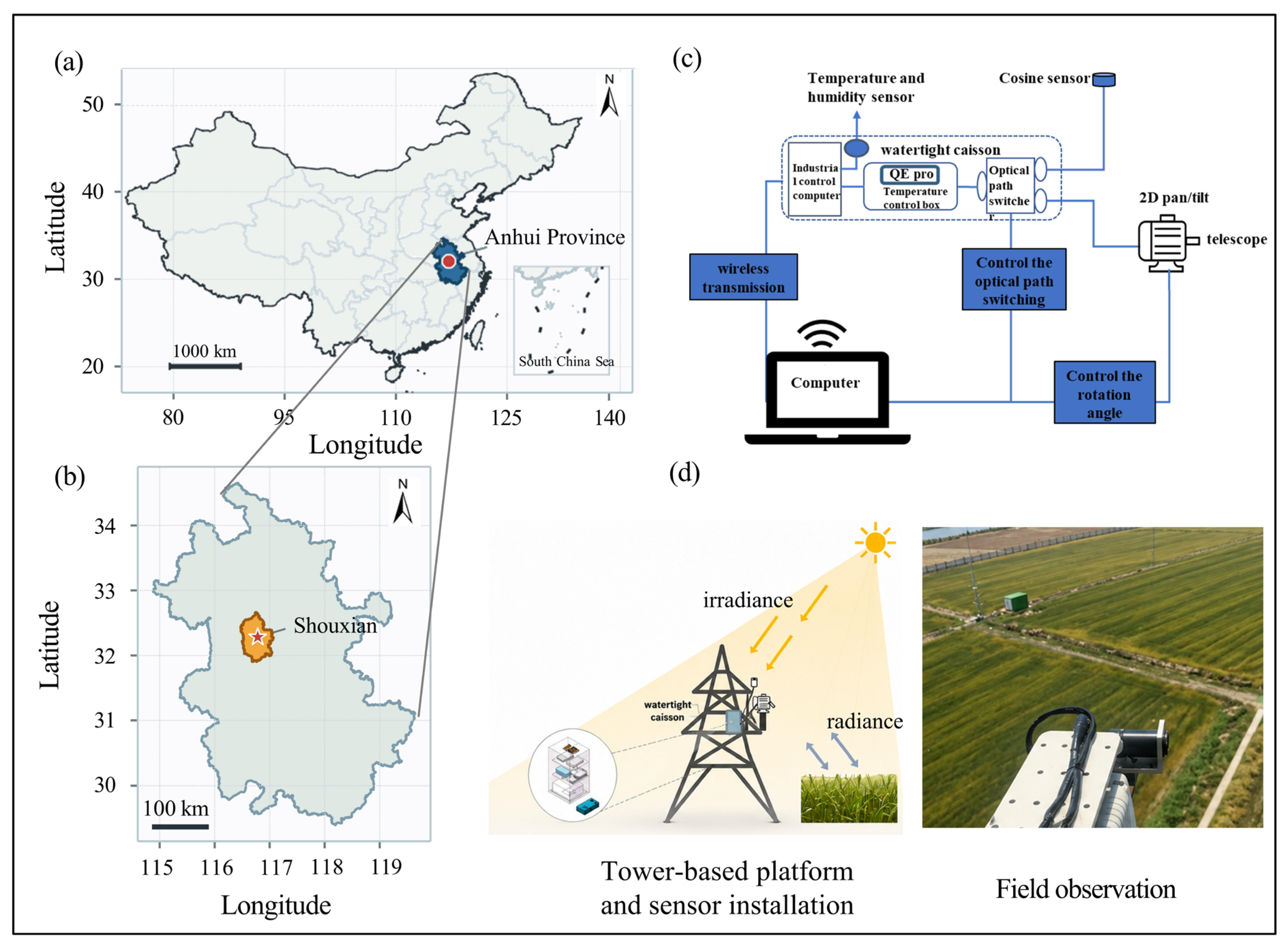
The DOAS-based algorithm described above requires high-resolution, radiometrically stable spectral measurements acquired continuously under field conditions. To meet these requirements and to enable automated long-term observation, we developed a dedicated tower-based SIF observation system, described below. In tower-based systems, spectrometers with a high signal-to-noise ratio and spectral resolution are typically employed. Through meticulous operation of the spectrometer, we can extract SIF signals from the spectral data. This system employs the QE Pro spectrometer, featuring TEC cooling, a high signal-to-noise ratio (1000:1), and high spectral resolution (0.3 nm). An optical path splitter divides the light path into two branches: one upward-facing branch connects to a cosine corrector with a 180° field of view, receiving sunlight; the other downward path connects to a telescope with a 1° field of view, mounted on a pan-tilt head capable of vertical and horizontal rotation to receive vegetation-emitted light from all directions. Instruments, including the spectrometer and switch, are housed within a waterproof enclosure to ensure stable operation under field conditions. An industrial control computer manages optical path switching, pan-tilt rotation angles, and data storage/transmission. The overall system configuration is illustrated in Figure 2c, while Figure 2d depicts the installation on an elevated tower in the field. Within this system, temperature and humidity sensors monitor internal environmental conditions. Two externally mounted cameras synchronously observe both vegetation growth within the site and the 2D pan-tilt unit’s rotational angles, facilitating remote monitoring of system operations. The industrial control computer incorporates a wireless network module, facilitating remote control, real-time monitoring of system status, and remote data transmission. Figure 2d also presents the on-site photos taken during the observation period in Shouxian County. The geographical location of Shouxian County is shown in Figure 2a,b.

The spectrometer underwent nonlinearity, dark current, and stray light testing. We employed a sixth-order polynomial to correct the nonlinearity of the QE Pro, thereby enhancing the instrument’s linearity. Dark current measurements were obtained by switching the optical path selector to its intermediate position, requiring separate measurements for the upper and lower optical paths. Each measurement set included one dark current measurement, which was subtracted during data preprocessing. In actual field observations, each measurement cycle followed a fixed sun–dark–vegetation–dark sequence: two upward-facing (solar) spectra were acquired and averaged, bracketing the downward-facing (vegetation) measurement, to minimise the time lag between the two channels (a “sandwich” acquisition scheme). Integration time was dynamically adjusted for each acquisition so that the peak signal reached approximately 60–80% of the spectrometer’s saturation level (200,000 counts for the QE Pro), balancing signal-to-noise ratio against a nonlinear response near saturation. Each measurement cycle took approximately 5 min to complete, and the system operated continuously from approximately 07:00 to 18:00 local time each day, yielding more than 100 measurement cycles per day under normal conditions.

To ensure the accuracy of measured absolute radiant intensities, the system requires frequent calibration. Initial laboratory calibration was performed separately for each channel. For the upward-facing channel measuring solar spectra, the cosine corrector was calibrated in a darkroom using an integrating sphere. The downward sensor with lens was calibrated using a standard whiteboard. For systems deployed long-term in the field, frequent laboratory calibration is impractical. Therefore, a cross-calibration method was adopted. A spectroradiometer already calibrated for radiation served as the reference. Both instruments simultaneously measured a diffuse reflector plate, and the radiation calibration factor for the system was calculated from the ratio of their signal intensities.

Theoretically, the SIF value for non-fluorescent surfaces should be zero. However, due to systematic errors, the measured SIF values are typically non-zero. Therefore, utilising the system’s pan/tilt rotation capability, we precisely observe non-fluorescent surfaces such as bare soil. By measuring the SIF values of a total of 100 non-fluorescent surfaces on different dates, the standard deviation of all the observed values was calculated as the background fluctuation; that is, the detection limit of this system is 0.071 mW/m²/nm/sr, which represents the observational uncertainty of the system.

2.4. Data Sources

2.4.1. Simulation Data

The SCOPE model (version 1.8) outputs solar and canopy spectra, which serve as input spectra for calculating the SIF value using a DOAS-based SIF retrieval method. Concurrently, the model-generated fluorescence serves as the ‘true’ value for validating the accuracy of the retrieval results. The SCOPE model operates at a default resolution of 1 nm. However, the Fraunhofer lines typically reside within narrow spectral bands, necessitating high-resolution outputs to resolve their minute spectral structures [21]. All downstream data processing—including generation of the noise-added simulation spectra, PCA, the DOAS retrieval algorithm, statistical analyses, and figure preparation—was performed in Python (version 3.11.6). For this purpose, it is necessary to change the resolution of the spectrum to adapt to the method we have proposed. By modifying the resolution of the leaf photochemical parameters and soil spectra in the SCOPE model input [24], we increased the resolution of the output parameters to 0.3 nm and ultimately obtained solar spectra and canopy spectra with a resolution of 0.3 nm.

However, the data output by SCOPE represents an idealised scenario and cannot simulate SIF retrieval under real-world conditions; in reality, spectrometers are inevitably subject to noise due to physical factors such as detector heat and photon randomness. We therefore artificially introduced noise into the SCOPE output spectra to simulate measurements from a real system. Following the method of Naethe et al., we first constructed the noise-equivalent radiation (NedL) to characterise the absolute radiative intensity of noise at different wavelengths; the calculation method is shown in Equation (10) [16]:

$$NedL\left(\lambda \right)={\displaystyle \frac{\sqrt{{\sigma }^2\left(N_{\lambda }\right)+{\sigma }^2\left(N_{\left(DC,\lambda \right)}\right)}}{IT}}\cdot g\left(\lambda \right)$$

(10)

where ${\sigma }^2\left(N_{\lambda }\right)$ and ${\sigma }^2\left(N_{\left(DC,\lambda \right)}\right)$ represent the standard deviations of the detector’s observed values under steady-state signal and dark-current conditions, respectively; $g\left(\lambda \right)$ (mW·m⁻²·nm⁻¹·sr⁻¹) represents the radiation calibration coefficient; and $IT$ (s) represents the integration time set during measurement, which is typically chosen such that the maximum light intensity reaches approximately 80% of the spectrometer’s saturation current. Next, the Monte Carlo simulation is used to introduce random Gaussian noise with a mean of 0 and a standard deviation of NedL. The noise constructed by this method can simulate the physical response of the instrument, and is closer to the noise of the actual instrument and the observation conditions.

2.4.2. Measured Data

The system conducted observational experiments at Hefei Science Island and the Anhui Shouxian National Climate Observatory, respectively. At Science Island, the observation target was trees, with the telescope positioned approximately 3 metres from the canopy. Daily observational experiments were carried out under varying weather conditions to compare different SIF retrieval methods. At Shouxian, the focus was on a winter wheat–rice rotation experimental field. The system was mounted on a meteorological observation tower, with the telescope situated roughly 20 metres above ground level. Installation and site imagery are shown in Figure 2. Long-term SIF observations of various crops were conducted at this location from May 2024 to August 2025, a period selected to span a complete wheat–rice rotation cycle: it began during the late growth stage of the 2023/2024 winter wheat, covered the full 2024 rice growing season, and continued through the subsequent 2024/2025 winter wheat season, thereby capturing the growth dynamics of both crops across more than one full rotation.

Prior to retrieval, spectra were excluded from further analysis under two conditions: (i) when the automatically adjusted integration time resulted in signal saturation; (ii) when the apparent reflectance spectrum failed to show the expected fluorescence-filling bulge near the 760 nm O₂–A absorption band—appearing instead flat or even depressed—indicating cloud-induced fluctuations in intensity and spectral structure between the paired upward and downward measurements within a cycle.

3. Results

3.1. Simulation Results

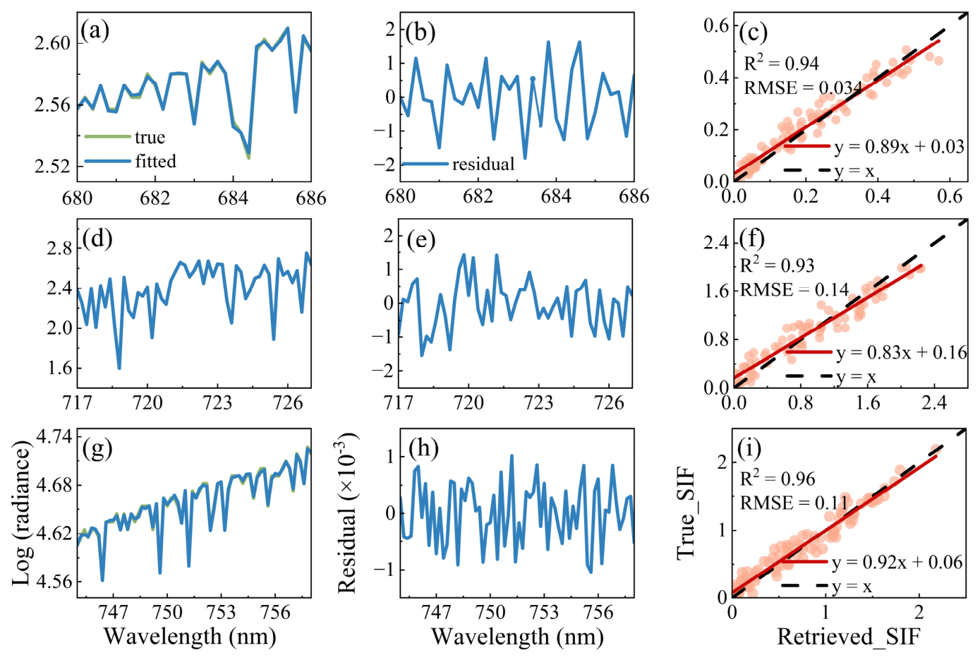
The retrieval method was first validated using simulated data. The gas absorption effect was incorporated into the retrieval simulation to mimic real tower conditions, focusing primarily on water vapour absorption. The accuracy of the fitting procedure was first evaluated. Figure 3a,d,g compare the logarithmic canopy spectra from SCOPE outputs with those fitted by the model, showing strong agreement across all bands. The corresponding residual plots (Figure 3b,e,h) exhibit no discernible structured patterns, indicating that the model parameters are well characterised. The root-mean-square (RMS) residuals, calculated across the three retrieval windows, were below 1.2 × 10⁻³ in the red band and below 1.4 × 10⁻³ in both the water vapour and far-red bands. These residuals reflect the combined effects of instrumental noise and polynomial fitting uncertainties. We further assessed the retrieval accuracy by correlating the SCOPE-simulated SIF (as reference) against the DOAS-retrieved SIF for 100 independent samples, generated from separate SCOPE parameter draws not included in the 1000-spectrum PCA reference library (Section 2.1.2), so that the retrieval validation is not circular with respect to the reference-spectrum construction. Figure 3c,f,i show that the retrieved values closely track the reference values across all samples, with correlation coefficients exceeding 0.9 in each window. These results demonstrate the high fidelity of the proposed retrieval method under controlled simulation conditions.

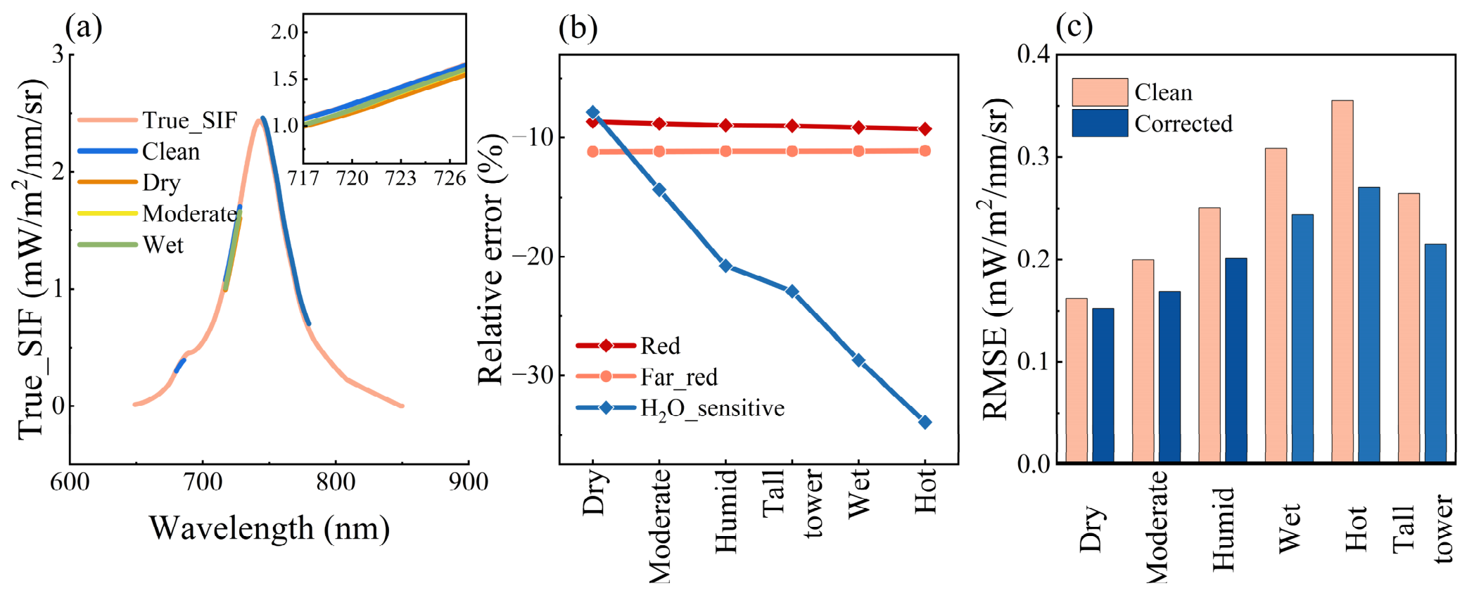
We further evaluated the influence of retrieval window selection and water vapour correction on SIF accuracy through two complementary analyses: window-dependent water vapour sensitivity and the effectiveness of correction under six temperature/humidity scenarios. Figure 4a compares the SIF spectra retrieved from different windows against the full-spectrum SCOPE reference. For the 717–727 nm window, results are shown for four conditions—clean (no water vapour), dry, moderate, and humid (see Section 2.2 for specific settings). All retrieved spectra closely match the reference shape. The red-band SIF values are consistently lower than those in the far-red bands, consistent with the known spectral properties of chlorophyll fluorescence. In healthy leaves, the red peak is attenuated by reabsorption as fluorescence propagates toward the leaf surface [25].

Figure 4b presents the relative retrieval errors across the three windows as a function of water vapour column density (six scenarios from dry to hot). The red (680–686 nm) and far-red (745–758 nm) windows show negligible water vapour sensitivity, with relative errors remaining near −9% and −11%, respectively, and varying by less than 1% across all scenarios. This small systematic bias likely arises from factors independent of atmospheric water vapour, such as reference spectral shape and polynomial fitting. In contrast, the 717–727 nm window exhibits strong water vapour sensitivity: its relative error increases monotonically with column density, from approximately −8% under dry conditions to −34% under hot, humid conditions. These results confirm that spectral window choice critically determines the susceptibility of SIF retrievals to water vapour interference, and that explicit correction is indispensable for windows with strong absorption features.

Figure 4c compares the retrieval RMSE before and after water vapour correction for the six scenarios within the 717–727 nm window. Correction reduces the RMSE in all cases, with the improvement increasing with water vapour loading. The reduction is minimal under dry conditions (from 0.16 to 0.15 mW·m⁻²·nm⁻¹·sr⁻¹), whereas the largest improvement occurs in the hot/humid scenario, where the RMSE decreases from 0.35 to 0.27 mW·m⁻²·nm⁻¹·sr⁻¹. These results demonstrate that the proposed correction effectively mitigates the systematic underestimation of SIF caused by water vapour absorption. Importantly, the correction provides greater accuracy gains under higher water vapour loads, ensuring robust retrieval performance under humid and thermally challenging conditions.

3.2. Measured Results

3.2.1. Comparison with Other Retrieval Methods

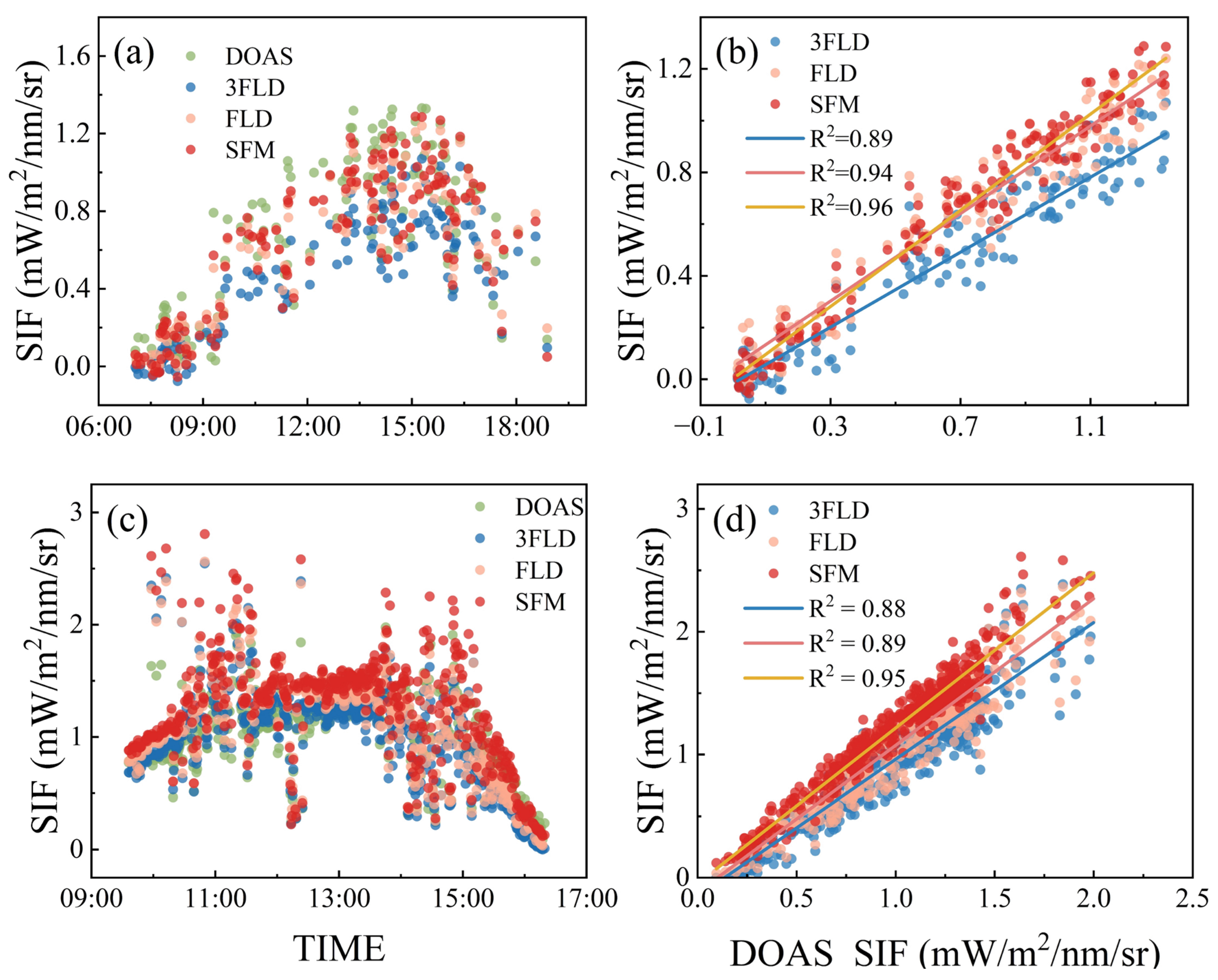
Field measurements were first conducted on tree canopies at Science Island using the tower-based SIF system, with the sensor mounted on a rooftop balcony approximately 3 m above the target canopy. Observations were made under both clear and cloudy conditions; Figure 5 shows the resulting SIF time series for each sky condition. To enable a consistent comparison across retrieval methods, the DOAS retrievals were projected onto a common reference at 760 nm via the fitted SIF spectrum.

Under clear skies, the SIF diurnal cycle follows a regular pattern, with low values in the early morning and late afternoon and a peak around midday. Under overcast conditions, the diurnal SIF variability increases substantially, owing to cloud-induced modifications of the incident solar spectrum. The downward solar spectrum measured by the upward channel exhibits strong scattering signatures from aerosols and clouds, with considerable temporal variation across different observation times. As noted by Guanter et al. [26], such elastic scattering effects can introduce errors in fluorescence retrievals. Despite these weather-induced variations, the correlations between the DOAS-based retrievals and conventional methods (FLD, 3FLD, SFM) consistently exceed 0.9 under both clear and cloudy conditions (Figure 5). We note that this comparison is not a fully independent validation, since all four methods (FLD, 3FLD, SFM, and DOAS) are derived from the same underlying spectral measurements; the implications of this are discussed further in Section 4.3.

To compare the stability of different retrieval methods under cloudy conditions, we computed the daily mean, standard deviation (SD), and coefficient of variation (CV = SD/mean) for the FLD, 3FLD, SFM, and DOAS retrievals (

Table 1. Mean, SD, and CV for daily observed SIF values retrieved by the 3FLD, FLD, SFM, and DOAS methods.

Retrieval Methods	Mean (mW·m−2·nm−1·sr−1)	SD (mW·m−2·nm−1·sr−1)	CV
3FLD	0.986	0.431	0.437
FLD	1.101	0.460	0.418
SFM	1.244	0.473	0.380
DOAS	1.021	0.364	0.356

). The DOAS method yields the lowest SD and CV among all methods, indicating that Fraunhofer line-based retrievals are more stable than O₂ band-based methods under overcast skies (see Section 4.3 for discussion of the extent to which this reflects window characteristics versus algorithmic performance).

3.2.2. Analysis of Diurnal and Long-Term Variation Trends

The simulation and short-term field comparisons above have demonstrated the effectiveness of the DOAS retrieval algorithm. To further evaluate its practical utility in real agricultural settings, we deployed the tower-based system at the Shouxian National Climate Observation Station from May 2024 to August 2025, covering a complete winter wheat–rice rotation cycle. This section examines the system’s ability to track crop phenology and investigates whether the DOAS-retrieved SIF captures the photosynthetic response of crops, as inferred from the diurnal dynamics of SIF and PAR and their lagged relationship.

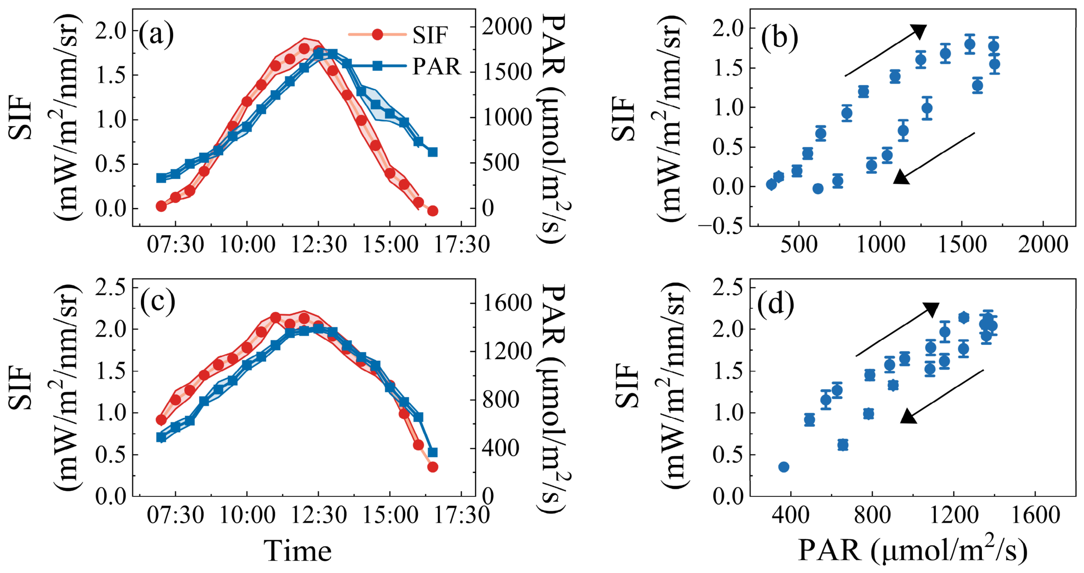
We analysed the diurnal SIF patterns for both wheat and rice during the rotation cycle. For both crops, SIF followed a consistent diurnal cycle, increasing from morning to a midday peak and then declining thereafter—a pattern primarily driven by photosynthetically active radiation (PAR). To quantify the SIF–PAR relationship, we measured diurnal PAR using sensors (Figure 6a,c; units: μmol m⁻² s⁻¹).

The diurnal SIF and PAR trends were broadly consistent, but their peak timings differed: the SIF maximum generally preceded the PAR peak (Figure 6a,c), suggesting a saturation effect of SIF under high light intensity. At midday, when solar irradiance is highest, photochemical reactions approach saturation; the absorbed light energy is then increasingly partitioned into non-photochemical quenching and fluorescence emission. As a result, SIF no longer increases linearly with PAR but instead saturates or even declines at high PAR levels (Figure 6b,d), consistent with the classic competition among photochemical quenching, thermal dissipation, and fluorescence emission [25].

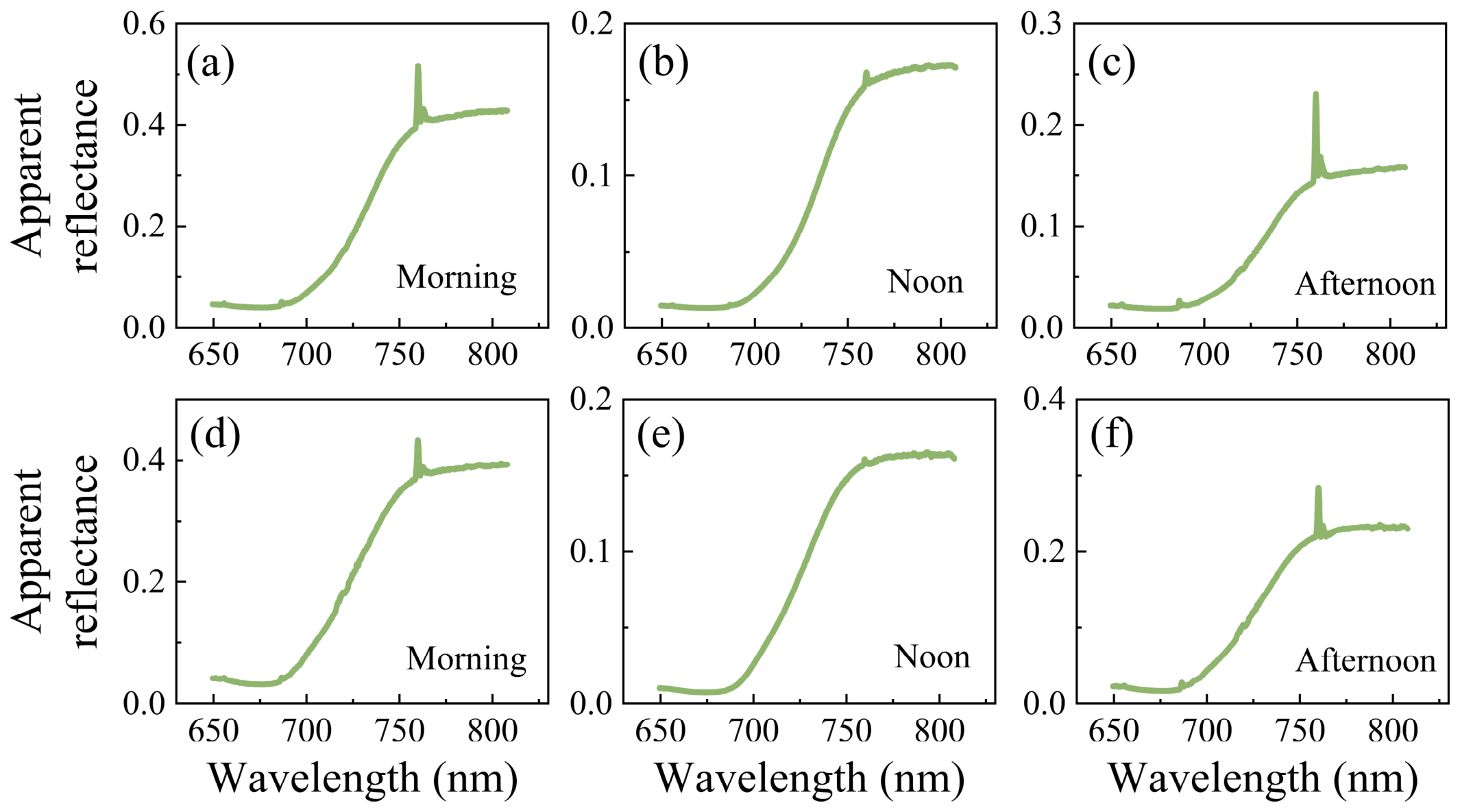
We also calculated the apparent reflectance at different times of day (morning, noon, and afternoon) from the measured spectra (Figure 7a–f). The reflectance at noon is lower than in the morning and afternoon, consistent with the known decrease in reflectance with increasing solar elevation angle. More notably, the apparent reflectance within the 760 nm O₂–A absorption band exhibits a reduced filling-in effect at noon compared to morning and afternoon, indicating that the relative SIF contribution to the upwelling radiance is smaller at midday. This observation further supports the saturation effect of SIF under high irradiance.

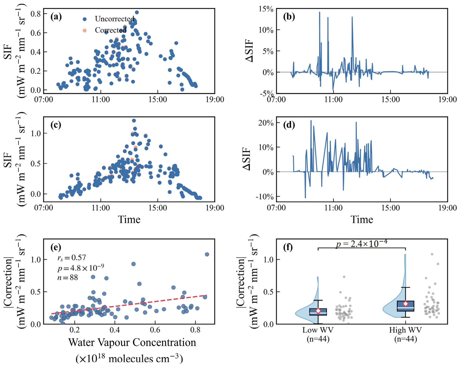
We further applied the DOAS retrieval to the water vapour-sensitive band (717–727 nm) on selected dates, with and without water vapour correction. Figure 8a,c compare the diurnal SIF cycles for the two cases, and Figure 8b,d show the corresponding relative differences. The SIF differences between corrected and uncorrected retrievals are generally within 20%. On all dates, the corrected SIF values are higher than the uncorrected ones, because water vapour absorption reduces the apparent filling-in depth, i.e., underestimates the SIF signal. The proposed correction scheme effectively addresses this bias.

The simulation experiments already demonstrated the accuracy of this method under controlled water vapour conditions. The field observations now provide independent verification under real atmospheric conditions. On 12 May 2025 (23 °C, 70% RH), the correction-induced difference was within ±2%; on 3 July 2025 (30 °C, 62% RH), it reached approximately 15%. This marked difference indicates that the correction magnitude scales with the actual water vapour column density along the path. The consistency between simulated and field-observed responses confirms that the water vapour effect in the 717–727 nm band is real and that the proposed correction is both necessary and effective. To go beyond these two examples, we conducted a further statistical analysis of the entire observational record. A total of 88 clear or partly cloudy days were selected, covering a range of atmospheric humidity conditions. By combining the synchronous temperature and relative humidity records with the Magnus equation and the ideal gas law (Section 2.2), we used the water vapour column density as an indicator of atmospheric water vapour loading (Figure 8e). On these days, the correction magnitude (the absolute difference between the gas-corrected and uncorrected SIF) increased monotonically with water vapour concentration (Spearman r = 0.57, p = 4.8 × 10⁻⁹), and was systematically larger on humid days than on dry days: when the records were divided by the median water vapour concentration, the correction magnitude on the more humid half of the days was significantly higher than on the drier half (Mann–Whitney U test, p = 2.4 × 10⁻⁴, n = 44 in each group), as shown in Figure 8f.

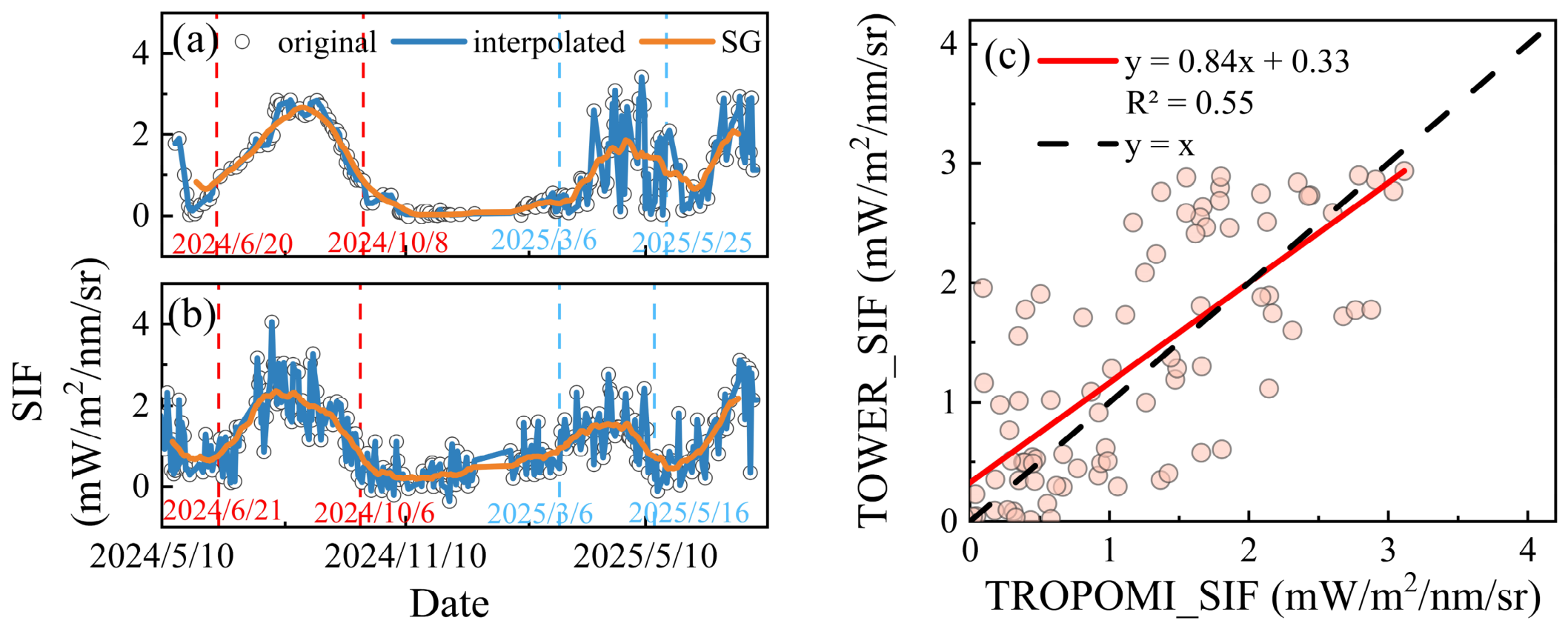
We further assessed the ability of our tower-based SIF retrievals to track crop phenology over the wheat–rice rotation. To enable a consistent comparison with TROPOMI, both SIF time series were gap-filled by temporal interpolation and smoothed with a Savitzky–Golay filter (window length: 31 days, third-order polynomial; Figure 9a,b). The two datasets are broadly consistent in their seasonal trajectories (Figure 9a,b), but show moderate point-to-point agreement (R² = 0.55, n = 189, p < 0.0001; Figure 9c). This moderate correlation is expected given the large difference in spatial support [27]. Each TROPOMI pixel (several kilometres) integrates heterogeneous land cover and fields at different phenological stages, whereas the tower footprint represents a small, relatively homogeneous canopy patch. Additional factors—including differences in overpass timing and satellite retrieval uncertainties—further limit the point-to-point correspondence. The R² of 0.55 falls within the range (0.47–0.59) reported for similar tower–satellite comparisons at native TROPOMI resolution [28,29]. Critically, despite this moderate agreement at the daily scale, both datasets capture the same seasonal phenological patterns, including the timing of green-up and senescence (Figure 9a,b). This indicates that the tower-based retrievals reproduce the phenological signal observed from space, and that the moderate R² primarily reflects scale mismatch rather than a deficiency in the retrieval algorithm.

We further extracted phenological metrics from the SG-filtered SIF time series. As winter-wheat SIF typically exhibits a bimodal pattern—with a first peak before winter dormancy and a second after spring regrowth [30]—we focused on the spring green-up period, which represents the main growing season [31]. Using a threshold-based approach commonly applied in phenological studies [32,33], we set the threshold at 20% of the seasonal amplitude based on comparison with field-observed growth stages: the start of season (SOS) was defined as the first day before the peak on which SIF exceeded this threshold, and the end of season (EOS) as the first day after the peak on which SIF fell below it. This approach was applied consistently to both tower-based and TROPOMI SIF time series to extract comparable phenological parameters, enabling the comparison of SOS and EOS between the two datasets.

As shown in Figure 9a,b, the rice phenological stages derived from tower-based observations were nearly identical to those from TROPOMI, whereas the SOS of winter wheat from the tower was 9 days later than that from the satellite. Field records indicate that the observed winter wheat did not begin regreening until early March, when photosynthetic activity started to rise. This discrepancy likely arises because phenological stages retrieved from coarse-resolution satellite pixels are influenced by surrounding vegetation with earlier SOS within the same grid cell [27]. Consequently, tower-based SIF provides a more accurate representation of local crop phenology, highlighting a key advantage of near-surface observations and their value as a benchmark for validating satellite-derived phenological products.

3.3. Sensitivity of SIF Retrieval to Reference Spectrum and Instrumental Noise

To assess whether the complexity of the SIF reference spectrum affects retrieval accuracy, we fixed the gas correction, polynomial order, and prior constraints in the DOAS-SIF framework and varied only the number of principal components (PCs) used in the reference spectrum, comparing the average spectrum (Mean), one principal component (PC1), two principal components (PC1–2), and three principal components (PC1–3). Extending the reference spectrum from a single averaged spectrum to three PCs changed the window-averaged SIF RMSE by less than 0.001% (

Table 2. Differences for each principal component relative to the three main components.

Comparison Combination	Absolute Difference in RMSE (mW·m−2·nm−1·sr−1)	Relative Difference in RMSE	Median Relative Error Difference
Mean vs. PC1–3	1.28 × 10−6	9.81 × 10−4%	3.51 × 10−3%
PC1 vs. PC1–3	1.28 × 10−6	9.83 × 10−4%	3.50 × 10−3%
PC1–2 vs. PC1–3	1.21 × 10−6	9.3 × 10−4%	3.37 × 10−3%

).

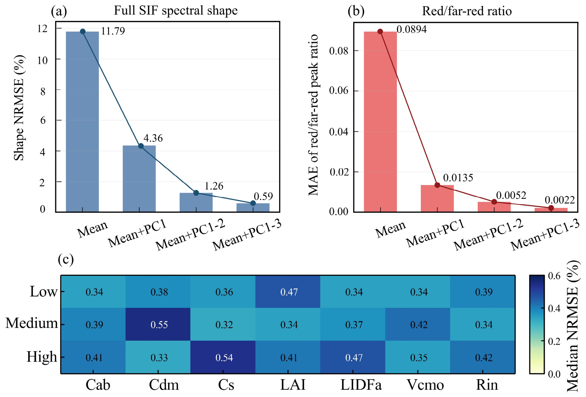
The window-averaged SIF error alone, however, does not fully capture the influence of the reference spectral shape on reconstructing the complete SIF spectrum. Using only the average spectral shape yields a normalised SIF spectrum RMSE (NRMSE) of 11.79%; adding PC1 reduces it to 4.36%, adding PC2 further lowers it to 1.26%, and adding PC3 brings it down to 0.59% (Figure 10a). Similarly, the absolute error of the red/far-red peak ratio decreases progressively from 0.0894 to 0.0022 as more PCs are included (Figure 10b).

To further evaluate the sensitivity of the PCA-based reference spectrum to the parameter sampling strategy, an independent validation dataset was generated using SCOPE parameter combinations not included in the PCA training library, and the reconstruction accuracy of the three-PC reference spectra was assessed across the key SCOPE input parameter subspaces considered in this study (the parameters hc, lw, and spectrum in Table A1 were fixed in the simulation setup and therefore not stratified into subgroups). The independent validation samples were grouped into low, medium, and high tertiles according to Cab, Cdm, Cs, LAI, LIDFa, Vcmo, and Rin. Values indicate the median normalised reconstruction RMSE (%) of the complete 650–850 nm SIF spectrum. On this independent validation set, the median RMSE for the full 650–850 nm SIF spectrum was 0.39%; slightly larger errors occurred in the medium Cdm, high Cs, and low LAI subspaces, but the median reconstruction error remained below 0.6% across all parameter subspaces (Figure 10c).

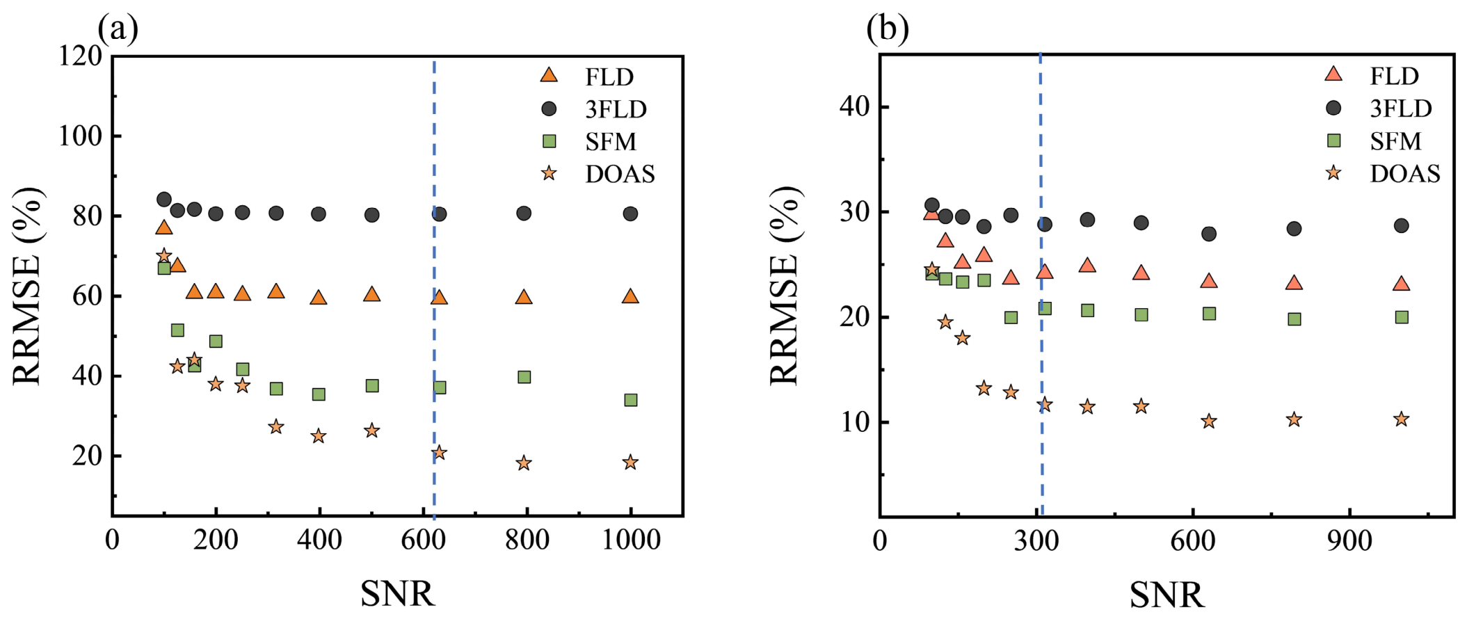
To characterise the method’s sensitivity to instrumental noise, artificial noise was added to the SCOPE output spectra in the simulation experiments (Section 2.4.1), and retrieval accuracy was quantified using the relative root-mean-square error (RRMSE) for the FLD, 3FLD, SFM, and DOAS-based retrievals in the red and far-red bands as a function of SNR (Figure 11a,b). Under the same spectral resolution, higher SNR consistently yields higher retrieval accuracy; the RRMSE approaches stability when SNR exceeds approximately 300 in the far-red band and 600 in the red band (as shown by the blue dotted line in Figure 11.). Among the four methods, the DOAS-based approach achieves the highest accuracy under identical instrument configurations, with RRMSE below 15% in the far-red band for SNR > 300.

4. Discussion

4.1. The Influence of the Reference Spectrum on the Retrieval Results

A fixed SIF reference spectrum represents only a typical fluorescence shape, whereas the actual canopy SIF spectrum varies with chlorophyll content, LAI, canopy structure, and illumination conditions—manifesting as relative changes in the red peak, far-red peak, and the valley between them [34,35]. To account for this variability, we constructed an adaptive reference spectrum using the SCOPE spectral library combined with PCA, representing SIF spectral variations with a limited number of principal components (PCs). As described in Section 2.1.2, PCA decomposition of the SCOPE SIF spectra (650–800 nm) showed that the first three PCs together explain 99.99% of the total spectral variance (PC1: 98.03%, PC1–PC2: 99.73%, PC1–PC3: 99.99%), indicating that they capture nearly all information relevant to SIF spectral shape variability. To assess whether the complexity of the reference spectrum affects retrieval accuracy, we fixed the gas correction, polynomial order, and prior constraints in the DOAS-SIF framework and varied only the number of PCs used in the reference spectrum.

These results (Section 3.3, Table 2) indicate that PC2 and PC3 have a negligible influence on the retrieved SIF amplitude within individual narrow windows, where the intensity is governed primarily by Fraunhofer line filling [36]. Nevertheless, the inclusion of PC2 and PC3 is essential for reconstructing the full SIF spectral shape, particularly the relative intensities of the red and far-red peaks and the intervening valley between them (Section 3.3, Figure 10a,b). These results demonstrate that PC2 and PC3 primarily improve the spectral adaptability of the reconstructed SIF—particularly in capturing the relative intensities of the red peak, far-red peak, and the valley between them—rather than altering the mean SIF amplitude within a single narrow window [37].

Having confirmed that the first three PCs adequately capture the main variability of the SIF spectral shape, we further evaluated the sensitivity of the PCA-based reference spectrum to the parameter sampling strategy using an independent validation dataset (Section 3.3). These results indicate that the extracted PCs do not overfit the original SCOPE dataset, and that the PCA-based reference spectra generalise well across a broad range of canopy biochemical, structural, and illumination conditions.

4.2. Method and System Advantages

The core contribution of this work is a DOAS-based retrieval framework that operates within Fraunhofer lines while actively correcting atmospheric interference. Its advantages over conventional methods are twofold. First, the simulation results show that this method can accurately retrieve the SIF signal in the water vapour band, and it performs well under different water vapour concentrations, and field measurements indicate that its stability is improved under cloudy conditions (with a lower CV value), solving the inherent vulnerability of the method based on the O₂ band to atmospheric changes [38,39]. Second, there is the construction of the reference SIF spectrum. Unlike previous empirical averaging approaches, our model-driven “SCOPE+PCA” method does not require measured spectral libraries, offering greater flexibility and transferability to diverse vegetation types. The SCOPE model can simulate SIF across a wide range of biochemical, structural, and stress conditions by varying its input parameters [40], whereas empirical averaging demands extensive field-measured SIF data from multiple species and environments. Our physically based strategy thus provides a more robust and generalisable foundation for SIF retrieval, as it captures the structural diversity of fluorescence spectra through process-based simulations rather than relying on statistical summaries of limited observations.

Compared with existing tower-based SIF systems, the present system combines several distinguishing characteristics. PhotoSpec pioneered narrow-field-of-view (0.7°), DOAS-based retrieval within Fraunhofer lines at very high spectral resolution (0.1 nm FWHM), demonstrating that this approach remains stable under cloudy conditions; however, its retrieval scheme deliberately avoids the water vapour absorption band, a gap this study addresses through explicit gas-phase correction. FLOX-type systems typically employ the same QE Pro spectrometer (0.3 nm FWHM) as used in this study, but with a much wider field of view (~23°) and retrieval based on FLD, iFLD, or SFM within the O₂ absorption bands rather than DOAS within Fraunhofer lines—the same class of methods against which our DOAS retrieval is benchmarked in Section 3.2.1. A recent systematic comparison of seven ground-based SIF retrieval algorithms, including DOAS, under varying water vapour conditions similarly found that O₂-band methods are more sensitive to atmospheric interference than Fraunhofer-line approaches [41], consistent with the present results. Relative to these systems, the present work combines PhotoSpec’s narrow-field DOAS/Fraunhofer-line approach with an active, physically based water vapour correction and a narrower field of view (1°) than FLOX-type systems, enabling more spatially resolved measurements while retaining robustness to the cloud and humidity effects that limit O₂-band methods.

Previous benchmarking studies have demonstrated that SIF retrieval accuracy is strongly affected by instrumental SNR and spectral resolution [42,43]. Consistent with this, our results (Section 3.3, Figure 8c,d) show that retrieval accuracy for all four methods improves with increasing SNR, with a minimum SNR of approximately 300 required for reliable SIF retrieval, and that the DOAS-based approach achieves the highest accuracy among the four methods under identical instrument configurations.

4.3. Limitations of This Study and Future Directions for Improvement

Several limitations of this study should be acknowledged. First, the reference SIF spectrum is model-based; future work could refine it by incorporating limited ground-truth measurements to further enhance its representativeness [44]. Second, as noted in Section 3.2.1, the inter-method comparison was not strictly equitable: FLD, 3FLD, and SFM operate in O₂ absorption bands, whereas our DOAS retrieval uses Fraunhofer-line windows. These spectral regions differ inherently in transmittance and scattering, so the lower CV of DOAS partly reflects window characteristics rather than unequivocal algorithmic superiority. A fully fair comparison would require implementing DOAS within the O₂ bands—a direction we plan to pursue in future work. Moreover, because all four methods are computed from the same underlying spectral measurements rather than from independent instruments or an independent reference SIF, their mutual agreement reflects relative consistency among retrieval algorithms rather than validated absolute accuracy, and should not be interpreted as evidence that any one method—including DOAS—retrieves the true SIF value. A genuinely independent validation would require comparison against an external reference not derived from the same spectral measurements, such as co-located eddy covariance-based GPP as a physiological proxy or a controlled fluorescence standard, which we identify as an important direction for future work. Nevertheless, the current comparison does confirm that Fraunhofer line-based strategies are more robust for tower-based SIF observations under cloudy and humid conditions, which constitute the primary operational scenario of this study. Third, while the method demonstrates robustness to water vapour, our tests have thus far been limited to water vapour-dominant bands; future work will extend the correction to additional absorption bands and ultimately enable full-spectrum SIF retrieval [45].

Similarly, the field validation in this study was conducted at two sites and two types of observations (trees at Science Island; crop at Shouxian); broader validation across additional sites and vegetation types would further strengthen confidence in the method’s generality. Finally, the comparison between tower-based and TROPOMI SIF (Section 3.2.2) is inherently limited by the large difference in spatial scale between a point-based tower footprint and a several-kilometre satellite pixel, which constrains the achievable point-to-point agreement independently of retrieval accuracy.

5. Conclusions

Tower-based SIF observations suffer from systematic retrieval errors due to atmospheric path interference between the sensor and canopy—a problem that conventional O₂-band-based FLD methods cannot adequately resolve under humid and cloudy conditions. To overcome this, we developed a DOAS-based retrieval algorithm that operates in Fraunhofer lines, constructs an adaptive reference spectrum via SCOPE+PCA, and actively corrects for atmospheric gas absorption. The algorithm is implemented in a dedicated tower-based system with a 1° scanning gimbal and high-resolution spectrometer.

Validation proceeded at three levels. Simulations confirmed accurate SIF retrieval, with correlation coefficients >0.9 across all windows. The 680–686 nm and 745–758 nm windows are stable against gas absorption, whereas the 717–727 nm window suffers from H₂O-induced bias that increases with humidity, temperature, and path length; the proposed correction reduced RMSE from 0.35 to 0.27 mW m⁻² nm⁻¹ sr⁻¹ under hot/humid conditions. Field comparisons showed the DOAS method to be more stable than FLD, 3FLD, and SFM under cloudy skies, with the lowest coefficient of variation, although this inter-method comparison is not fully independent, as all four methods are derived from the same underlying spectral measurements. A field campaign spanning 88 clear-sky days further confirmed that the water-vapour correction magnitude increases significantly with atmospheric water-vapour loading (r = 0.57, p = 4.8 × 10⁻⁹), corroborating the simulation-based results.

A 15-month wheat–rice field campaign demonstrated the system’s practical value: retrieved SIF captured consistent seasonal phenological dynamics with TROPOMI (R² = 0.55, n = 189), despite the expected scale mismatch between tower and satellite footprints, and captured SIF–PAR lag and midday saturation effects. The multi-window DOAS framework provides a reliable solution for automated, high-precision tower-based SIF observation under complex atmospheric conditions, and lays a foundation for future full-spectrum retrieval.

References

1. McFarlane, J.C.; Watson, R.D.; Theisen, A.F.; Jackson, R.D.; Ehrler, W.L.; Pinter, P.J.; Idso, S.B.; Reginato, R.J. Plant Stress Detection by Remote Measurement of Fluorescence. Appl. Opt. 1980, 19, 3287–3289. [Google Scholar] [CrossRef] [Scilit] [PubMed]
2. Alonso, L.; Gomez-Chova, L.; Vila-Frances, J.; Amoros-Lopez, J.; Guanter, L.; Calpe, J.; Moreno, J. Improved Fraunhofer Line Discrimination Method for Vegetation Fluorescence Quantification. IEEE Geosci. Remote Sens. Lett. 2008, 5, 620–624. [Google Scholar] [CrossRef] [Scilit]
3. Carter, G.A.; Jones, J.H.; Mitchell, R.J.; Brewer, C.H. Detection of Solar-Excited Chlorophyll a Fluorescence and Leaf Photosynthetic Capacity Using a Fraunhofer Line Radiometer. Remote Sens. Environ. 1996, 55, 89–92. [Google Scholar] [CrossRef] [Scilit]
4. Maier, S.W. Remote Sensing and Modelling of Solar Induced Fluorescence. ESA Spec. Publ. 2002, 527, 6. [Google Scholar]
5. Yang, X.; Tang, J.; Mustard, J.F.; Lee, J.-E.; Rossini, M.; Joiner, J.; Munger, J.W.; Kornfeld, A.; Richardson, A.D. Solar-Induced Chlorophyll Fluorescence That Correlates with Canopy Photosynthesis on Diurnal and Seasonal Scales in a Temperate Deciduous Forest. Geophys. Res. Lett. 2015, 42, 2977–2987. [Google Scholar] [CrossRef] [Scilit]
6. Zhang, Y.; Zhang, Q.; Liu, L.; Zhang, Y.; Wang, S.; Ju, W.; Zhou, G.; Zhou, L.; Tang, J.; Zhu, X.; et al. ChinaSpec: A Network for Long-Term Ground-Based Measurements of Solar-Induced Fluorescence in China. J. Geophys. Res. Biogeosciences 2021, 126, e2020JG006042. [Google Scholar] [CrossRef] [Scilit]
7. Yang, H.; Yang, X.; Zhang, Y.; Heskel, M.A.; Lu, X.; Munger, J.W.; Sun, S.; Tang, J. Chlorophyll Fluorescence Tracks Seasonal Variations of Photosynthesis from Leaf to Canopy in a Temperate Forest. Glob. Change Biol. 2017, 23, 2874–2886. [Google Scholar] [CrossRef] [Scilit] [PubMed]
8. Sabater, N.; Middleton, E.M.; Malenovsky, Z.; Alonso, L.; Verrelst, J.; Huemmrich, K.F.; Campbell, P.K.E.; Kustas, W.P.; Vicent, J.; Van Wittenberghe, S.; et al. Oxygen Transmittance Correction for Solar-Induced Chlorophyll Fluorescence Measured on Proximal Sensing: Application to the NASA-GSFC Fusion Tower. In Proceedings of the 2017 IEEE International Geoscience and Remote Sensing Symposium (IGARSS), Fort Worth, TX, USA, 23–28 July 2017; pp. 5826–5829. [Google Scholar]
9. Sabater, N.; Vicent, J.; Alonso, L.; Verrelst, J.; Middleton, E.M.; Porcar-Castell, A.; Moreno, J. Compensation of Oxygen Transmittance Effects for Proximal Sensing Retrieval of Canopy–Leaving Sun–Induced Chlorophyll Fluorescence. Remote Sens. 2018, 10, 1551. [Google Scholar] [CrossRef] [Scilit] [PubMed]
10. Grossmann, K.; Frankenberg, C.; Magney, T.S.; Hurlock, S.C.; Seibt, U.; Stutz, J. PhotoSpec: A New Instrument to Measure Spatially Distributed Red and Far-Red Solar-Induced Chlorophyll Fluorescence. Remote Sens. Environ. 2018, 216, 311–327. [Google Scholar] [CrossRef] [Scilit]
11. Köhler, P.; Guanter, L.; Joiner, J. A Linear Method for the Retrieval of Sun-Induced Chlorophyll Fluorescence from GOME-2 and SCIAMACHY Data. Atmos. Meas. Tech. 2015, 8, 2589–2608. [Google Scholar] [CrossRef] [Scilit]
12. Guanter, L.; Rossini, M.; Colombo, R.; Meroni, M.; Frankenberg, C.; Lee, J.-E.; Joiner, J. Using Field Spectroscopy to Assess the Potential of Statistical Approaches for the Retrieval of Sun-Induced Chlorophyll Fluorescence from Ground and Space. Remote Sens. Environ. 2013, 133, 52–61. [Google Scholar] [CrossRef] [Scilit]
13. Wieneke, S.; Burkart, A.; Cendrero-Mateo, M.P.; Julitta, T.; Rossini, M.; Schickling, A.; Schmidt, M.; Rascher, U. Linking Photosynthesis and Sun-Induced Fluorescence at Sub-Daily to Seasonal Scales. Remote Sens. Environ. 2018, 219, 247–258. [Google Scholar] [CrossRef] [Scilit]
14. Middleton, E.M.; Rascher, U.; Corp, L.A.; Huemmrich, K.F.; Cook, B.D.; Noormets, A.; Schickling, A.; Pinto, F.; Alonso, L.; Damm, A.; et al. The 2013 FLEX—US Airborne Campaign at the Parker Tract Loblolly Pine Plantation in North Carolina, USA. Remote Sens. 2017, 9, 612. [Google Scholar] [CrossRef] [Scilit]
15. Zhao, F.; Li, R.; Verhoef, W.; Cogliati, S.; Liu, X.; Huang, Y.; Guo, Y.; Huang, J. Reconstruction of the Full Spectrum of Solar-Induced Chlorophyll Fluorescence: Intercomparison Study for a Novel Method. Remote Sens. Environ. 2018, 219, 233–246. [Google Scholar] [CrossRef] [Scilit]
16. Naethe, P.; Julitta, T.; Chang, C.Y.-Y.; Burkart, A.; Migliavacca, M.; Guanter, L.; Rascher, U. A Precise Method Unaffected by Atmospheric Reabsorption for Ground-Based Retrieval of Red and Far-Red Sun-Induced Chlorophyll Fluorescence. Agric. For. Meteorol. 2022, 325, 109152. [Google Scholar] [CrossRef] [Scilit]
17. Stutz, J.; Platt, U. Numerical Analysis and Estimation of the Statistical Error of Differential Optical Absorption Spectroscopy Measurements with Least-Squares Methods. Appl. Opt. 1996, 35, 6041–6053. [Google Scholar] [CrossRef] [Scilit] [PubMed]
18. van der Tol, C.; Verhoef, W.; Timmermans, J.; Verhoef, A.; Su, Z. An Integrated Model of Soil-Canopy Spectral Radiances, Photosynthesis, Fluorescence, Temperature and Energy Balance. Biogeosciences 2009, 6, 3109–3129. [Google Scholar] [CrossRef] [Scilit]
19. Verrelst, J.; Rivera, J.P.; van der Tol, C.; Magnani, F.; Mohammed, G.; Moreno, J. Global Sensitivity Analysis of the SCOPE Model: What Drives Simulated Canopy-Leaving Sun-Induced Fluorescence? Remote Sens. Environ. 2015, 166, 8–21. [Google Scholar] [CrossRef] [Scilit]
20. Kohavi, R. A Study of Cross-Validation and Bootstrap for Accuracy Estimation and Model Selection. In Proceedings of the Proceedings of the 14th International Joint Conference on Artificial intelligence; Morgan Kaufmann Publishers Inc.: San Francisco, CA, USA, 1995; Volume 2, pp. 1137–1143. [Google Scholar]
21. Verhoef, W.; van der Tol, C.; Middleton, E.M. Hyperspectral Radiative Transfer Modeling to Explore the Combined Retrieval of Biophysical Parameters and Canopy Fluorescence from FLEX—Sentinel-3 Tandem Mission Multi-Sensor Data. Remote Sens. Environ. 2018, 204, 942–963. [Google Scholar] [CrossRef] [Scilit]
22. Rothman, L.S. History of the HITRAN Database. Nat. Rev. Phys. 2021, 3, 302–304. [Google Scholar] [CrossRef] [Scilit]
23. Gueymard, C.A.; Myers, D.; Emery, K. Proposed Reference Irradiance Spectra for Solar Energy Systems Testing. Sol. Energy 2002, 73, 443–467. [Google Scholar] [CrossRef] [Scilit]
24. Yang, P.; Prikaziuk, E.; Verhoef, W.; van der Tol, C. SCOPE 2.0: A Model to Simulate Vegetated Land Surface Fluxes and Satellite Signals. Geosci. Model Dev. 2021, 14, 4697–4712. [Google Scholar] [CrossRef] [Scilit]
25. Mohammed, G.H.; Colombo, R.; Middleton, E.M.; Rascher, U.; van der Tol, C.; Nedbal, L.; Goulas, Y.; Pérez-Priego, O.; Damm, A.; Meroni, M.; et al. Remote Sensing of Solar-Induced Chlorophyll Fluorescence (SIF) in Vegetation: 50 years of Progress. Remote Sens. Environ. 2019, 231, 111177. [Google Scholar] [CrossRef] [Scilit] [PubMed]
26. Guanter, L.; Alonso, L.; Gómez-Chova, L.; Meroni, M.; Preusker, R.; Fischer, J.; Moreno, J. Developments for Vegetation Fluorescence Retrieval from Spaceborne High-Resolution Spectrometry in the O2-A and O2-B Absorption Bands. J. Geophys. Res. Atmos. 2010, 115, D19303. [Google Scholar] [CrossRef] [Scilit]
27. Zhang, X.; Wang, J.; Gao, F.; Liu, Y.; Schaaf, C.; Friedl, M.; Yu, Y.; Jayavelu, S.; Gray, J.; Liu, L.; et al. Exploration of Scaling Effects on Coarse Resolution Land Surface Phenology. Remote Sens. Environ. 2017, 190, 318–330. [Google Scholar] [CrossRef] [Scilit]
28. Hu, J.; Jia, J.; Ma, Y.; Liu, L.; Yu, H. A Reconstructed Global Daily Seamless SIF Product at 0.05 Degree Resolution Based on TROPOMI, MODIS and ERA5 Data. Remote Sens. 2022, 14, 1504. [Google Scholar] [CrossRef] [Scilit]
29. Hu, J.; Jia, J.; Ma, Z.; Yuan, K.; Yu, H.; Liu, L. A Spatially Downscaled TROPOMI SIF Product at 0.005° Resolution with Bias Correction. IEEE J. Sel. Top. Appl. Earth Obs. Remote Sens. 2024, 17, 13413–13425. [Google Scholar] [CrossRef] [Scilit]
30. Liu, Y.; Wan, H.; Guo, P.; Liu, W.; Han, Z.; Jiao, Y. Quantifying Winter Wheat Phenology Patterns in the North China Plain Using Solar-Induced Chlorophyll Fluorescence. Agric. Water Manag. 2025, 320, 109885. [Google Scholar] [CrossRef] [Scilit]
31. White, M.A.; De Beurs, K.M.; Didan, K.; Inouye, D.W.; Richardson, A.D.; Jensen, O.P.; O’keefe, J.; Zhang, G.; Nemani, R.R.; Van Leeuwen, W.J.D.; et al. Intercomparison, Interpretation, and Assessment of Spring Phenology in North America Estimated from Remote Sensing for 1982–2006. Glob. Change Biol. 2009, 15, 2335–2359. [Google Scholar] [CrossRef] [Scilit]
32. Gan, L.; Cao, X.; Chen, X.; Dong, Q.; Cui, X.; Chen, J. Comparison of MODIS-Based Vegetation Indices and Methods for Winter Wheat Green-up Date Detection in Huanghuai Region of China. Agric. For. Meteorol. 2020, 288–289, 108019. [Google Scholar] [CrossRef] [Scilit]
33. Liu, L.; Cao, R.; Chen, J.; Shen, M.; Wang, S.; Zhou, J.; He, B. Detecting Crop Phenology from Vegetation Index Time-Series Data by Improved Shape Model Fitting in Each Phenological Stage. Remote Sens. Environ. 2022, 277, 113060. [Google Scholar] [CrossRef] [Scilit]
34. Rossini, M.; Meroni, M.; Celesti, M.; Cogliati, S.; Julitta, T.; Panigada, C.; Rascher, U.; Van der Tol, C.; Colombo, R. Analysis of Red and Far-Red Sun-Induced Chlorophyll Fluorescence and Their Ratio in Different Canopies Based on Observed and Modeled Data. Remote Sens. 2016, 8, 412. [Google Scholar] [CrossRef] [Scilit]
35. Balde, H.; Hmimina, G.; Goulas, Y.; Latouche, G.; Ounis, A.; Soudani, K. Data-Based Investigation of the Effects of Canopy Structure and Shadows on Chlorophyll Fluorescence in a Deciduous Oak Forest. Biogeosciences 2024, 21, 1259–1276. [Google Scholar] [CrossRef] [Scilit]
36. Sun, Y.; Frankenberg, C.; Jung, M.; Joiner, J.; Guanter, L.; Köhler, P.; Magney, T. Overview of Solar-Induced Chlorophyll Fluorescence (SIF) from the Orbiting Carbon Observatory-2: Retrieval, Cross-Mission Comparison, and Global Monitoring for GPP. Remote Sens. Environ. 2018, 209, 808–823. [Google Scholar] [CrossRef] [Scilit]
37. Li, S.; Gao, M.; Li, Z.-L.; Labed, J.; Verhoef, W. FSM: A Reflectance Reconstruction Method to Retrieve Full-Spectrum Sun-Induced Chlorophyll Fluorescence from Canopy Measurements. IEEE Trans. Geosci. Remote Sens. 2024, 62, 5540816. [Google Scholar] [CrossRef] [Scilit]
38. Chang, C.Y.; Guanter, L.; Frankenberg, C.; Köhler, P.; Gu, L.; Magney, T.S.; Grossmann, K.; Sun, Y. Systematic Assessment of Retrieval Methods for Canopy Far-Red Solar-Induced Chlorophyll Fluorescence Using High-Frequency Automated Field Spectroscopy. J. Geophys. Res. Biogeosciences 2020, 125, e2019JG005533. [Google Scholar] [CrossRef] [Scilit]
39. Daumard, F.; Goulas, Y.; Ounis, A.; Pedrós, R.; Moya, I. Measurement and Correction of Atmospheric Effects at Different Altitudes for Remote Sensing of Sun-Induced Fluorescence in Oxygen Absorption Bands. IEEE Trans. Geosci. Remote Sens. 2015, 53, 5180–5196. [Google Scholar] [CrossRef] [Scilit]
40. Pacheco-Labrador, J.; Perez-Priego, O.; El-Madany, T.S.; Julitta, T.; Rossini, M.; Guan, J.; Moreno, G.; Carvalhais, N.; Martín, M.P.; Gonzalez-Cascon, R.; et al. Multiple-Constraint Inversion of SCOPE. Evaluating the Potential of GPP and SIF for the Retrieval of Plant Functional Traits. Remote Sens. Environ. 2019, 234, 111362. [Google Scholar] [CrossRef] [Scilit]
41. Zhang, Y.; Liu, X.; Du, S.; Qi, M.; Jing, X.; Liu, L. Performance of Ground-Based Solar-Induced Chlorophyll Fluorescence Retrieval Algorithms at the Water Vapor Absorption Band. Sensors 2025, 25, 689. [Google Scholar] [CrossRef] [Scilit] [PubMed]
42. Liu, L.; Liu, X.; Hu, J. Effects of Spectral Resolution and SNR on the Vegetation Solar-Induced Fluorescence Retrieval Using FLD-Based Methods at Canopy Level. Eur. J. Remote Sens. 2015, 48, 743–762. [Google Scholar] [CrossRef] [Scilit]
43. Cendrero-Mateo, M.P.; Wieneke, S.; Damm, A.; Alonso, L.; Pinto, F.; Moreno, J.; Guanter, L.; Celesti, M.; Rossini, M.; Sabater, N.; et al. Sun-Induced Chlorophyll Fluorescence III: Benchmarking Retrieval Methods and Sensor Characteristics for Proximal Sensing. Remote Sens. 2019, 11, 962. [Google Scholar] [CrossRef] [Scilit]
44. Liu, W.; Mõttus, M.; Malenovský, Z.; Shi, S.; Alonso, L.; Atherton, J.; Porcar-Castell, A. An In Situ Approach for Validation of Canopy Chlorophyll Fluorescence Radiative Transfer Models Using the Full Emission Spectrum. Remote Sens. Environ. 2025, 316, 114490. [Google Scholar] [CrossRef] [Scilit]
45. Zhao, F.; Tariq, M.; Ma, W.; Wu, Z.; Zhang, Y. An Enhanced Method for Reconstruction of Full SIF Spectrum for Near-Ground Measurements. Int. J. Appl. Earth Obs. Geoinf. 2024, 134, 104240. [Google Scholar] [CrossRef] [Scilit]
Figure 1. (a) Fluorescence spectrum simulated using SCOPE (the number of samples = 1000 spectra; a representative subset is shown); (b) the first three principal components (PC1: 98.03%, PC2: 99.73%, PC3: 99.99%), accounting for 99.99% of the total variance; (c) SIF spectra synthesised from these components with different coefficients; (d) high-resolution water vapour absorption spectrum from HITRAN; (e) Gaussian fitting of the measured mercury lamp peak; (f) convolved effective water vapour absorption cross-section; (g) solar spectrum (650–800 nm) showing typical Fraunhofer lines and the retrieval window (blue shading: the three retrieval windows, green shading: optimal water vapour window); (h) mean absolute relative error of SIF retrieval across different water vapour-sensitive sub-windows.
Remotesensing 18 02837 g001
Figure 2. Location map of the tower-based SIF system observation: (a) geographic location of the Shouxian station in China; (b) geographic location of the Shouxian station in Anhui Province. (c) System architecture diagram of the SIF tower-based observation system. (d) On-site deployment illustration and field observation diagram.
Remotesensing 18 02837 g002
Figure 3. For the red, water vapour-sensitive, and far-red bands: (a,d,g) logarithmic canopy spectra output by SCOPE (real values) and fitted by the model (fitted values); (b,e,h) fitting residuals; (c,f,i) correlation between retrieved and true values for 100 samples in each band.
Remotesensing 18 02837 g003
Figure 4. (a) Retrieved and SCOPE-output SIF spectra; (b) relative errors for the three bands; (c) RMSE before and after correction (Clean/Corrected) within the water vapour-sensitive band.
Remotesensing 18 02837 g004
Figure 5. Retrieved results under different weather conditions. Under clear weather conditions, (a) the SIF retrieved results, and (b) the correlation between the SIF results retrieved by the DOAS method and those calculated by other methods (FLD, 3FLD, SFM; Pearson r > 0.9). Under cloudy weather conditions, (c) the SIF retrieved results, and (d) the correlation between the SIF results retrieved by the DOAS method and those calculated by other methods.
Remotesensing 18 02837 g005
Figure 6. (a,c) Daily variation curves of SIF and PAR; (b,d) changes in SIF with PAR throughout the day (the arrow indicates the change of time throughout the day). (a,b) Rice observations on 28 July 2024; (c,d) wheat observations on 23 April 2025.
Remotesensing 18 02837 g006
Figure 7. Representative examples of apparent reflectance spectra at different times of the day: (ac) spring, during the wheat green-up period (23 April 2025); (df) rice, approaching maturity in early autumn (3 September 2024).
Remotesensing 18 02837 g007
Figure 8. Comparison of SIF with and without water vapour correction: (a,c) daily SIF trends and (b,d) relative differences before and after correction for 12 May 2025 (23 °C, 70% RH (a,b)) and 3 July 2025 (30 °C, 62% RH; (c,d)); (e) statistical analysis of the correlation between SIF correction amplitude and water vapour concentration; (f) distribution of SIF correction for the low water vapour group and the high water vapour group.
Remotesensing 18 02837 g008
Figure 9. Time series of (a) tower-based SIF and (b) TROPOMI SIF from May 2024 to August 2025, and (c) their comparison (R2 = 0.55, n = 189, p < 0.0001). In (a,b), red and blue dotted lines mark the SOS and EOS dates of rice and wheat, respectively.
Remotesensing 18 02837 g009
Figure 10. The influence of principal component selection on SIF spectral reconstruction; (a) normalised RMSE (NRMSE, %) of the reconstructed SIF spectrum as a function of the number of principal components used; (b) mean absolute error of the red/far-red peak intensity ratio; (c) generalisation of the three-PC PCA-SIF reference spectrum across SCOPE parameter subspaces, evaluated on an independent validation set not used in PCA construction.
Remotesensing 18 02837 g010
Figure 11. At different signal-to-noise ratios (SNRs), the relative RMSE (RRMSE, %) of the retrieval results obtained by FLD, 3FLD, SFM, and DOAS methods at (a) the red band and (b) the far-red band.
Remotesensing 18 02837 g011