Mirrored Aperture Synthesis Radiometric Imaging Based on Spatial Bandpass Sampling and Quad-Beam Antennas: Design and Numerical Validation

Highlights

What are the main findings?

• Shifting the imaging region from the incident angle of 0° to the oblique direction of (θ = 45°, ϕ = 45°) can mitigate the oversized reflector issue in 2-D MAS.
• The shifted imaging region can be regarded as a spatial bandpass signal, and the spatial bandpass sampling theorem is more suitable. A quad-beam antenna pattern better matches the spatial bandpass case.

What are the implications of the main findings?

• 2-D MAS based on spatial bandpass sampling and quad-beam antenna can use small-sized reflectors to realize BT distribution image reconstruction.
• 2-D MAS based on spatial bandpass sampling and quad-beam antennas can guarantee proper array size and antenna gain.

Abstract

Mirrored aperture synthesis radiometry (MAS) has been proposed for passive microwave remote sensing with high spatial resolution and relatively few antenna elements. However, low incident angles and improper azimuth angles result in oversized reflectors, posing difficulties for practical deployment. To address this issue, the center of the imaging region is shifted from the incident angle of 0° to the oblique direction of (θ = 45°, ϕ = 45°) in this paper, which is quite different from conventional aperture synthesis radiometry architecture. The problem of oversized reflectors and the necessity of shifting the imaging region are discussed. To match the shifted imaging region, a new design scheme based on spatial bandpass sampling and quad-beam antennas for MAS imaging is proposed. Instead of the Nyquist baseband sampling adopted in conventional aperture synthesis, the spatial bandpass sampling is adopted to process the spatial bandpass signal caused by the imaging region shift. Then, antennas with quad-beam pattern are proposed and designed to receive the incident wave and three reflected waves. Numerical simulation experiments are conducted to demonstrate the feasibility of the proposed method. This work focuses on the conceptual design and principle validation, and does not involve hardware implementation or prototype fabrication.

1. Introduction

Both Europe and China have successfully launched spaceborne L-band aperture synthesis radiometers to sense sea surface salinity and soil moisture with high spatial resolution [1,2,3,4], which is also applied in sea ice thickness and wind speed remote sensing [5]. In addition, researchers in Europe are exploring more advanced L-band aperture synthesis radiometers to further improve spatial resolution to meet the application requirements of meso-scale ocean physics study, water resources management, food security, and other fields [6]. Meanwhile, researchers in Europe, America, and China have proposed geostationary aperture synthesis radiometers for real-time sounding of atmospheric parameters with continuous regional coverage in next-generation geostationary satellite missions, represented by GeoSTAR [7], GAS [8], and GIMS [9]. Aperture synthesis technology provides an alternative to real aperture for remote sensing at low microwave frequencies or in high orbit, and it has been attracting increasing attention.

However, compared with real aperture radiometry, the advantage of aperture synthesis radiometry is at the cost of high system complexity and complicated signal processing. For example, GAS adopts a stationary array of 2500 elements or a rotating Y-shaped array of 450 elements [8]. To reduce the computational pressure and power consumption of cross-correlation processing, one-bit correlators are applied in aperture synthesis radiometers, resulting in a certain loss in sensitivity.

In [10,11], mirrored aperture synthesis (MAS) was proposed to reduce the system complexity by decreasing the number of antennas. As the combination of the two-element interferometer and the Lloyd’s mirror interferometer, due to the presence of the reflectors, I/Q demodulation is not required in MAS, which simplifies the receiver structure and reduces the number of correlators. Some related issues have been investigated, such as antenna design and antenna arrangement of the mirrored antenna array [12,13,14,15], the relationship between mirrored aperture synthesis and aperture synthesis [16], and the reconstruction algorithms [17,18]. In addition, a V-band MAS prototype has been developed to verify the fundamentals of MAS [11].

In [19], the reflector dimensions for 2-D MAS were discussed. When the incident angle of scene radiation is small, large-sized reflectors are needed to receive reflected waves, which makes practical application difficult. In order to reduce the dimensions of the two reflectors in 2-D MAS, the center of the image region is shifted from the incident angle of 0° to the oblique direction of $(\theta =45°, \varphi =45°)$ in this paper. To match this specific feature, a dedicated design scheme integrating spatial bandpass sampling and quad-beam antennas for MAS radiometry is proposed.

This paper first provides a brief overview of the fundamentals of 2-D MAS. The problem of oversized reflectors and the necessity of shifting the imaging region are discussed. Second, the Nyquist baseband sampling theorem and bandpass sampling theorem are introduced. The shifted imaging region is treated as a spatial bandpass signal, and spatial bandpass sampling is applied to determine the proper sampling frequency or repetition period in the spatial domain. Third, to match the shifted imaging region, quad-beam antennas are designed and discussed. At last, proof-of-principle numerical simulations are conducted to demonstrate the feasibility of the proposed design. It should be clarified that this work does not involve hardware implementation or prototype retrofitting, which will be further addressed in future work.

2. Materials and Methods

2.1. A Brief Overview of the Fundamentals of 2-D MAS

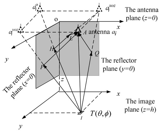
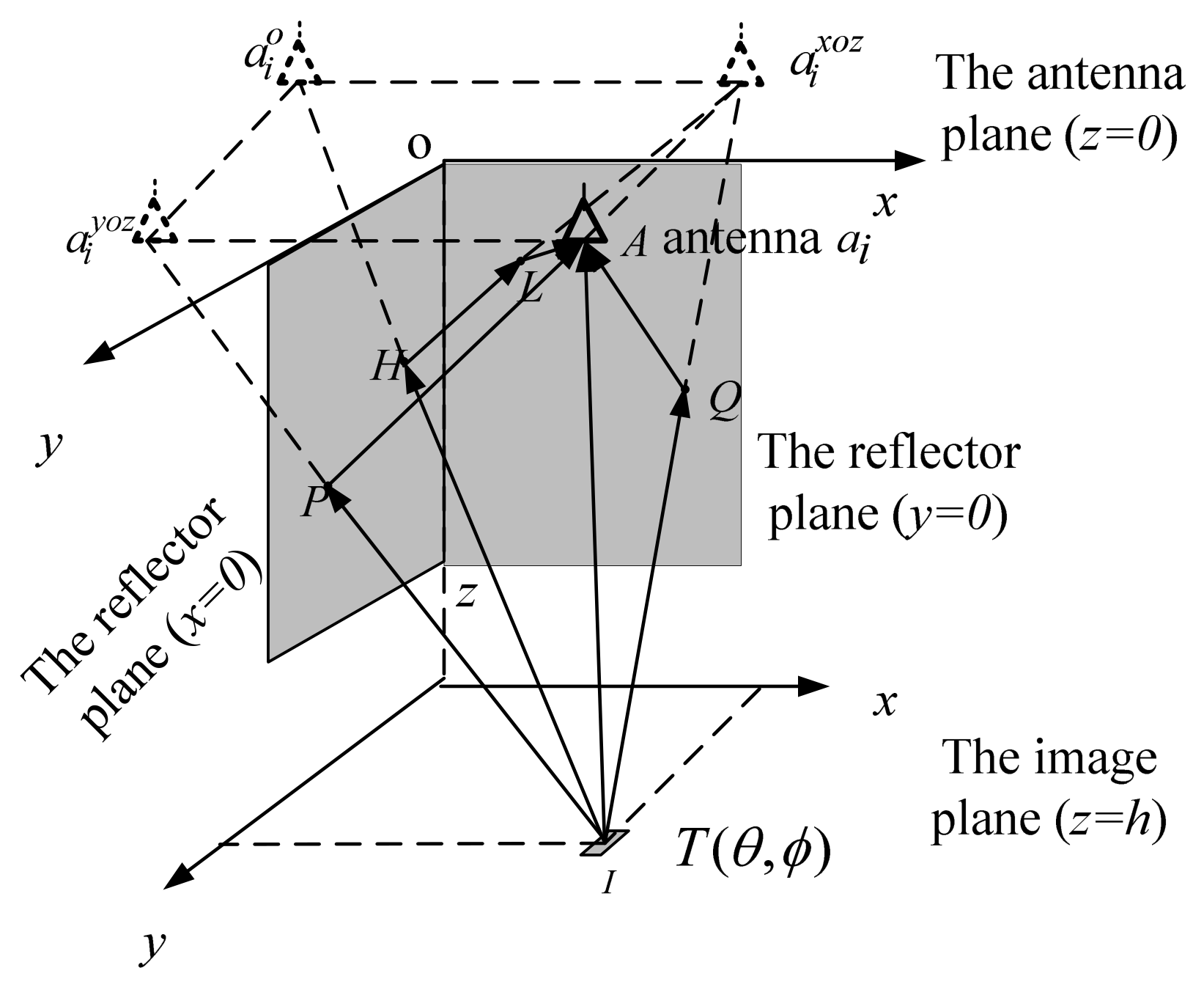
As shown in Figure 1, a 2-D MAS radiometer primarily consists of two planar reflectors and an array receiver equipped with a 2-D array [20]. The two reflectors are positioned in the YOZ plane and XOZ plane, respectively, while the 2-D array is placed in the XOY plane. For any imaging pixel in the scene with a 2-D brightness temperature (BT) distribution, each antenna in a 2-D MAS radiometer receives not only the direct signal emitted by the pixel but also the three reflected signals from the two reflectors. The first reflected signal comes from the wave propagating toward the reflector located in the YOZ plane. The second reflected signal comes from the wave propagating toward the reflector in the XOZ plane. The third reflected signal is generated through the double reflection from the two reflectors. From another perspective, the existence of the two reflectors forms three mirrored antennas for each antenna, namely $a_i^{xoz}$, $a_i^{yoz}$, and $a_i^o$. For an antenna with the coordinate $\left(x_i{, y}_i\right)$, the coordinates of the three mirrored antennas are $\left(x_i{,- y}_i\right)$, $\left({-x}_i{, y}_i\right)$, and $\left({-x}_i{,- y}_i\right)$, respectively.

Figure 1. The geometry and the illustration of 2-D MAS. Reprinted with permission from [20]. Copyright 2026 IEEE.

Based on the above description, the signal received by a single antenna can be expressed as follows:

$$b\left(t\right)=b^d\left(t\right)+b^{yoz}\left(t\right)+b^{xoz}\left(t\right)+b^o\left(t\right)$$

(1)

where $t$ is time, and the superscript $d$, $yoz$, $xoz$, and $o$ denote the direct signal and three reflected signals, respectively. For any two arbitrary antennas $a_i$ and $a_j$, the cross-correlation output of the received signals for linear polarization along the y direction is [11]:

$$\begin{array}{c}{R}_{ij}=⟨b_i\left(t\right)b_j^{*}\left(t\right)⟩=C_V\left(x_j-x_i,y_j-y_i\right)+C_V\left(x_j-x_i,y_j+y_i\right)\\ -C_V\left(x_j+x_i,y_j-y_i\right)-C_V\left(x_j+x_i,y_j+y_i\right)\end{array}$$

(2)

where $\left(\xi =\mathit{sin}\theta \mathit{cos}\varphi ,\eta =\mathit{sin}\theta \mathit{sin}\varphi \right)$ are the direction cosines, $T\left(\xi ,\eta \right)=T_{\Omega }\left(\xi ,\eta \right)/\sqrt{1-{\xi }^2-{\eta }^2}$ denotes the 2-D modified BT, and $(u,v)$ is the 2-D spatial frequency. The relationship between the modified BT distribution and the cosine visibility is characterized by a 2-D cosine transform. When there are S antenna elements, a matrix can be constructed to describe the relationship between the cosine visibilities and all cross-correlation outputs:

$$\left[\begin{array}{c}{R}_{12}\\ R_{13}\\ ⋮\\ R_{\left(S-1\right)S}\end{array}\right]=\left[\begin{array}{cccccc}1& 1& \cdots & -1& -1& 0\\ ⋮& 1& \cdots & -1& -1& 0\\ ⋮& ⋮& ⋮& ⋮& ⋮& ⋮\\ 0& 1& \cdots & -1& 0& -1\end{array}\right]\left[\begin{array}{c}{C}_V\left(\mathrm{0,1}\right)\\ C_V\left(\mathrm{0,2}\right)\\ ⋮\\ C_V\left(M,N\right)\end{array}\right]$$

(3)

where M and N are the number of spatial frequencies in two dimensions, respectively. The linear equations mentioned above can be simplified into the following compact form:

$$\mathbf{R}=\mathbf{P}·{\mathbf{C}}_{\mathbf{V}}$$

(4)

Each row in matrix P is determined by the following conditions:

$${\mathbf{P}}_{ij}\left(m,n\right)=\left\{\begin{array}{cc}\hfill 1,& (m,n)=\left(\right|x_j-x_i|,|y_j-y_i\left|\right)\hfill \\ \hfill 1,& (m,n)=\left(\right|x_j-x_i|,|y_j+y_i\left|\right)\hfill \\ \hfill -1,& \left(m,n\right)=\left(\left|x_j+x_i\right|,\left|y_j-y_i\right|\right)\hfill \\ \hfill -1,& \left(m,n\right)=\left(\left|x_j+x_i\right|,\left|y_j+y_i\right|\right)\hfill \\ \hfill 0,& \mathrm{otherwise}\hfill \end{array}\right.$$

(5)

The cosine visibilities can be derived by solving Equation (3), and the BT distribution image can be reconstructed from these cosine visibilities via a 2-D inverse cosine transform, which is expressed as:

$$T(\xi ,\eta )=4{\int }_0^{\infty }{\int }_0^{\infty }{C}_V(u,v)\mathit{cos}(2\pi u\xi )\mathit{cos}(2\pi v\eta )dudv$$

(6)

2.2. Reflector Dimensions for 2-D MAS

As shown in Figure 1, the reflected waves reflected by the reflector and then received by the real antenna a_i can be equivalently regarded as being received by the corresponding mirror antennas $a_i^{xoz}$ and $a_i^{yoz}$, respectively. The positions of the two reflection points P and Q are determined by the coordinates of $a_i^{xoz}$ and $a_i^{yoz}$. The reflected wave with double reflection can be equivalently received by the mirror antenna $a_i^o$, and the positions of reflection points H and L on the reflectors are determined by the coordinate of $a_i^o$.

For a certain pixel in the imaging region, a larger coordinate of the real antenna leads to longer distances between the mirrored antennas and reflectors. In this case, the reflector points P and Q move downward along the z direction, which means larger reflector dimensions are required.

In addition, the positions of reflection points are also affected by the direction $(\theta , \varphi )$ of the pixel. A qualitative analysis is conducted as follows. When $\varphi$ approaches 0, the pixel point is closer to the x-axis. As the incident wave impinges on the reflector in the XOZ plane, the local incident angle with respect to the reflector increases, resulting in a larger dimension of the reflector along the z direction. Similarly, as $\varphi$ approaches $\pi /2$, the required dimension of the reflector in the YOZ plane along the z-axis also increases. Furthermore, a smaller $\theta$ indicates the pixel is closer to the z-axis, resulting in a larger local incident angle with respect to the two reflectors. The dimension of the two reflectors along the z direction both increases. Therefore, to achieve a reasonable dimensional design of the reflectors, the imaging region should be constrained within proper ranges of $\theta$ and $\varphi$.

In [19], the dimensions of two reflectors are analyzed based on solid geometry, and the values are determined by the antenna coordinate $\left(x_i{, y}_i\right)$ and the direction $(\theta , \varphi )$, as detailed below:

$$D_{xoz}=\left\{\begin{array}{cc}\{2x_i, {\displaystyle \frac{y_{i}cot \theta }{sin \varphi }}\}& \varphi \le {\tan }^{-1}{\displaystyle \frac{y_i}{x_i}}\\ \{2y_{i}cot \varphi , {\displaystyle \frac{y_{i}cot \theta }{sin \varphi }}\}& \varphi >{\tan }^{-1}{\displaystyle \frac{y_i}{x_i}}\end{array}\right.$$

(7)

$$D_{yoz}=\left\{\begin{array}{cc}\{2x_{i}tan \varphi , {\displaystyle \frac{x_{i}cot \theta }{\mathrm{c}\mathrm{o}\mathrm{s} \varphi }}\}& \varphi \le {\tan }^{-1}{\displaystyle \frac{y_i}{x_i}}\\ \{2y_i, {\displaystyle \frac{x_{i}cot \theta }{cos \varphi }}\}& \varphi >{\tan }^{-1}{\displaystyle \frac{y_i}{x_i}}\end{array}\right.$$

(8)

where $D_{xoz}$ and $D_{yoz}$ represent the dimensions of the reflector in the XOZ plane and that in the YOZ plane. It can be found that one reflector dimension is inversely proportional to $sin \varphi$, while the other is inversely proportional to $cos \varphi$. This means that a tradeoff between the dimensions of the two reflectors must be considered, and $\varphi =45°$ is a good candidate. Similarly, $\theta =45°$ is a good candidate too. Accordingly, the image region should be centered at $(\theta =45°, \varphi =45°)$. From the perspective of direction cosines, the direction of the imaging center corresponds to $\left(\xi =0.5,\eta =0.5\right)$.

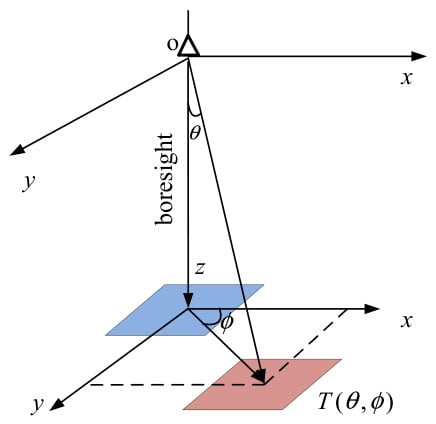
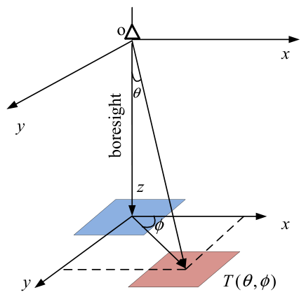
Figure 2 further illustrates the geometric layout of the imaging regions in the antenna frame. For a conventional aperture synthesis radiometer, the center of the imaging region is generally in the incident angle of $0°$ indicated by the blue square. However, in order to reduce the dimensions of the two reflectors in MAS, the center of the imaging region is recommended at $(\theta =45°, \varphi =45°)$, indicated by the red square.

Figure 2. The geometric relationship between the imaging region and the antenna in the antenna frame. Original imaging region is indicated by the blue square, and the shifted imaging region is indicated by the red square.

Let us compare the required dimensions of the reflectors before and after the imaging region shift. For a conventional MAS radiometer, its imaging region is restricted to the neighborhood of the coordinate origin and in the first quadrant of the image plane. We take the coordinates of the antenna farthest from the origin in the antenna plane as (1 m, 1 m), and consider a neighborhood centered at the coordinate origin in the image plane with a maximum incident angle of $8°$. According to (7) and (8), pixels within this neighborhood that have small incident angles $\theta$ and azimuth angles $\varphi$ approaching $0°$ and $90°$ will lead to extremely large reflector dimensions. For instance, for the pixel in the neighborhood with the incident direction $\left(\theta =0.5°, \varphi =0.5°\right)$, the required dimensions of the two reflectors are approximately (2 m, 13,131 m) and (0.0175 m, 114.593 m), respectively. For the pixel with the incident direction $\left(\theta =0.5°, \varphi =89.5°\right)$, the corresponding required reflector dimensions are approximately (0.0175 m, 114.593 m) and (2 m, 13,131 m). Thus, for a conventional MAS radiometer, the required height for the two reflectors exceeds 1000 m, which is difficult for practical deployment.

When the imaging region is shifted to $\left(\theta =45°, \varphi =45°\right)$, the incident angle and azimuth angle ranges of the imaging region are restricted on the interval $37°\le \theta , \varphi \le 53°$. Among all pixels in this region, the pixels with the incident direction ($\theta =$ 37°, $\varphi$ = 37°) and ($\theta =$ 37°, $\varphi$ = 53°) require the largest reflector dimensions. For ($\theta =$ 37°, $\varphi$ = 37°), the dimensions of the two reflectors derived from (7) and (8) are (2 m, 2.205 m) and (1.507 m, 1.662 m), respectively. For the pixel (37°, 53°), the corresponding reflector dimensions are (1.507 m, 1.662 m) and (2 m, 2.205 m), respectively. It can be found the maximum height for the two reflectors is 2.205 m, which is much smaller than the required size for a conventional MAS radiometer. Therefore, the dimensions of the reflectors can be greatly reduced by shifting the imaging region.

2.3. Spatial Bandpass Sampling for 2-D MAS

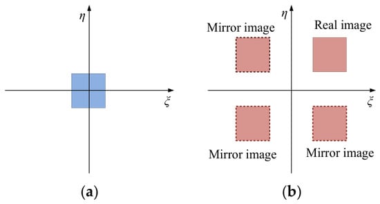
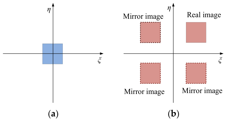
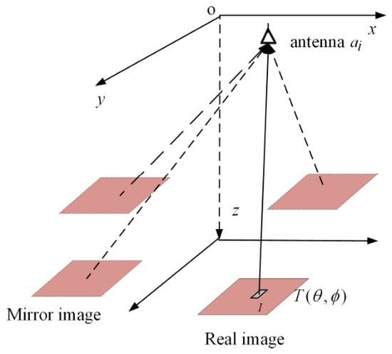
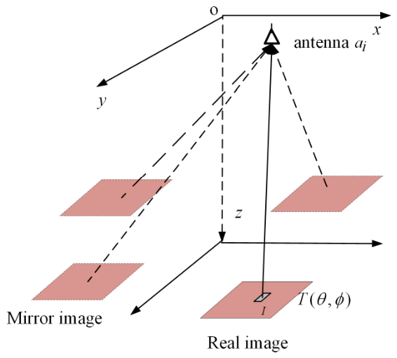
In Figure 3, the imaging regions are redrawn on the plane spanned by $\xi$ and $\eta$. Figure 3a corresponds to the conventional aperture synthesis. The imaging region is within a square region centered at the origin, which can be treated as a 2-D baseband signal. Thus, the conventional Nyquist sampling theorem can be applied for spatial sampling. Figure 3b corresponds to the 2-D MAS. For $(\theta =45°, \varphi =45°)$, the corresponding direction cosines are $(\xi =0.5, \eta =0.5)$. The real imaging region is in the first quadrant centered at $(\xi =0.5, \eta =0.5)$. And due to the presence of the two reflectors, each antenna in 2-D MAS will receive the direct signal and three reflected signals. The three reflected signals can be regarded as direct incident signals for the three mirror images in the other three quadrants. In this case, the imaging region cannot be treated as a 2-D baseband signal and should instead be characterized as a 2-D bandpass signal.

Figure 3. An illustration of the imaging regions in the plane spanned by $\xi$ and $\eta$. (a) The baseband case; (b) the bandpass case.

For both conventional aperture synthesis and MAS, the $\xi \eta$ domain and the $uv$ domain are related by Fourier transform. The antenna arrangement determines the $uv$ distribution, and the minimum antenna spacing determines the minimum spatial frequency sample in the $uv$ plane, thereby determining the repetition period in the $\xi \eta$ plane. According to the Nyquist sampling theorem, to achieve alias-free sampling, the 2-D repetition periods ${\xi }_s$ and ${\eta }_s$ must be greater than the maximum coverage range of the imaging region in the two spatial dimensions.

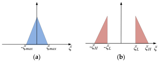
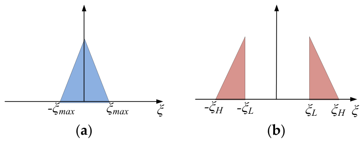
For convenience, a 1-D case is illustrated in Figure 4. For the baseband case in Figure 4a, when ${\xi }_s\ge 2{\xi }_{max}$ holds, the reconstructed image has no aliasing. For example, if ${\xi }_{max}$ equals 1, ${\xi }_s$ should be greater than 2, and the corresponding minimum antenna spacing normalized with respect to wavelength is ${\displaystyle \frac{1}{2}}$. This is why ${\displaystyle \frac{\lambda }{2}}$ is required for no aliasing or no ambiguity in array signal processing. For a bandpass case in Figure 4b, if the Nyquist sampling theorem is applied, ${\xi }_s$ should be greater than $2{\xi }_H$, leading to a small antenna spacing $\Delta u=1/{\xi }_s$. Thus, the array size will be reduced and the spatial resolution will degrade. The element antenna gain will decrease, and the system sensitivity will also be affected. A better sampling method is adopting the bandpass sampling theorem to replace the conventional Nyquist sampling theorem. By exploiting the gap between ${-\xi }_L$ and ${\xi }_L$, it enables sampling at a lower rate. Generally, the candidate for ${\xi }_s$ can be denoted as follows [21]:

$${\displaystyle \frac{2{\xi }_H}{k}}\le {\xi }_s\le {\displaystyle \frac{2{\xi }_L}{k-1}}$$

(9)

where $k\in \{\mathrm{1,2},3\dots \}$ has an integer value. According to Equation (9), the value for k is:

$$1\le k\le {\displaystyle \frac{{\xi }_H}{{\xi }_H-{\xi }_L}}$$

(10)

Figure 4. An illustration for 1-D baseband sampling and bandpass sampling. (a) The baseband case; (b) the bandpass case.

In practice, ${\xi }_s$ is typically set to its minimum value to maximize the antenna spacing $\Delta u=1/{\xi }_s$. This allows a larger array aperture, thereby improving spatial resolution. It means k should be taken as the maximum integer. Substituting the maximum k into Equation (9) yields the minimum ${\xi }_s$. For example, given ${\xi }_L=0.4$ and ${\xi }_H=0.6$, the maximum value for k is 3. Substituting these values into Equation (9), the minimum ${\xi }_s$ is 0.4, and the wavelength-normalized antenna spacing is $2.5$. In contrast, if the Nyquist sampling theorem for the baseband case is adopted, ${\xi }_s$ is 1.2 and the normalized antenna spacing is $1/1.2$, which is much smaller than 2.5.

For the 2-D case shown in Figure 3b, there are two repetition periods along $\xi$ and $\eta$, respectively. And the candidates for ${\xi }_s$ and ${\eta }_s$ can be calculated by Equation (9), respectively. Then, the wavelength-normalized antenna spacing along each dimension is given by $1/{\xi }_s$ and $1/{\eta }_s$, respectively.

Another problem is how to determine ${\xi }_H$ when the normalized antenna spacing is $\Delta u$. According to Equation (9), the boundary of ${\xi }_L$ and ${\xi }_H$ can be determined:

$$\begin{array}{c}{\xi }_L\ge {\displaystyle \frac{k-1}{2}}{\xi }_s\\ {\xi }_H\le {\displaystyle \frac{k}{2}}{\xi }_s\end{array}$$

(11)

Thus, the largest field of view (FOV) is obtained by:

$$\begin{array}{c}{\xi }_L={\displaystyle \frac{k-1}{2}}{\xi }_s\\ {\xi }_H={\displaystyle \frac{k}{2}}{\xi }_s\end{array}$$

(12)

On the other hand, to minimize reflector dimensions, the imaging region is centered at $(\xi =0.5, \eta =0.5)$, yielding:

$${\xi }_L+{\xi }_H=\left(k-0.5\right){\xi }_s=2\ast 0.5$$

(13)

Hence:

$$k={\displaystyle \frac{1}{{\xi }_s}}+0.5=\Delta u+0.5$$

(14)

Since k is an integer, the optimal value of the normalized antenna spacing $\Delta u$ takes the form of $k-0.5$, such as 1.5, 2.5, 3.5, and so on. Similarly, (11)–(14) are applicable to describe the relationship among ${\eta }_s$, ${\eta }_L$, and ${\eta }_H$.

2.4. Quad-Beam Antennas for 2-D MAS

For the shifted imaging region, if a traditional antenna with one main beam is applied, the antenna beam should be wide enough to cover the shifted imaging region, and the antenna gain will decrease. To match the feature of the imaging region shift and spatial bandpass sampling, the antennas should be redesigned for 2-D MAS.

Another imaging equivalence for 2-D MAS is shown in Figure 5. The three reflected waves in Figure 1 are equivalent to three direct incident waves emitted from three mirror images of the real image. Therefore, antennas in 2-D MAS should have a symmetric four-beam antenna pattern with the directions of maximum gain at $(\theta =45°, \varphi =45°)$, $(\theta =45°, \varphi =135°)$, $(\theta =45°, \varphi =225°)$, and $(\theta =45°, \varphi =315°)$, respectively. It is quite different from the conventional antenna pattern in array signal processing and aperture synthesis radiometry.

Figure 5. Imaging equivalence for 2-D MAS: one real image and three mirror images.

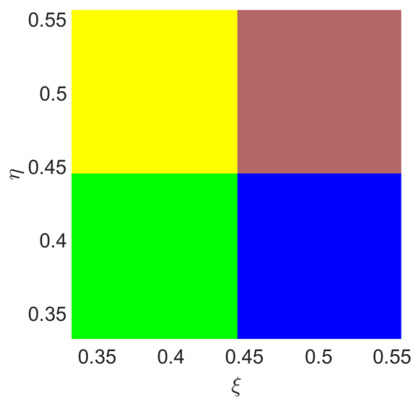
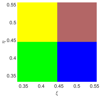
According to (14), given k = 5, $\Delta u=4.5$ and $\Delta v=4.5$ can be obtained. The two sampling repetition periods ${\xi }_s$ and ${\eta }_s$ in the $\xi \eta$ domain both equal 0.2222. Then, according to (12) and (13), the values of ${\xi }_H$ and ${\xi }_L$ are 0.5556 and 0.4444. In the same manner, the values for ${\eta }_H$ and ${\eta }_L$ are 0.5556 and 0.4444. Let us consider a square imaging region centered at (0.5, 0.5), with the four vertices at $(\xi =0.4444, \eta =0.4444)$, $(\xi =0.4444, \eta =0.5556)$, $(\xi =0.5556, \eta =0.4444)$, and $(\xi =0.5556, \eta =0.5556)$, respectively. Its three mirror images are square regions centered at (−0.5, 0.5), (0.5, −0.5), and (−0.5, −0.5), respectively. According to the sampling theorem, the imaging region and its three mirror images are periodically extended and replicated across the image plane. One of the periodic extensions of the imaging region and its three mirror images is illustrated in Figure 6. The red region is the imaging region. The yellow region is the extension of the mirror image centered at (−0.5, 0.5), extending along the $\xi$ direction by $4{\xi }_s$. The blue region is the extension of the mirror image centered at (0.5, −0.5), extending along the $\eta$ direction by $4{\eta }_s$. The green region is the extension of the mirror image centered at (−0.5, −0.5), extending along the two directions by $4{\xi }_s$ and $4{\eta }_s$, respectively. It can be found that there is no aliasing when the imaging region is restricted in the interval $0.4444\le \xi , \eta \le 0.5556$. If the imaging region is enlarged, aliasing will occur, but aliasing-free imaging can be achieved by reducing the antenna spacing.

Figure 6. One of the periodic extensions of the imaging region and its three mirror images. The red region is the imaging region. The yellow, blue, and green regions are the periodic extensions of its three mirror imaging regions respectively. No aliasing occurs.

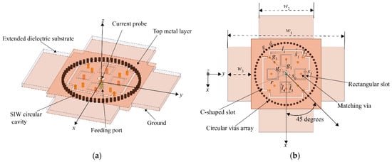
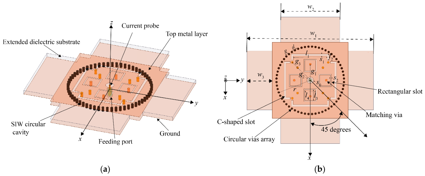
Figure 7 illustrates the configuration of the proposed quad-beam antenna. The center frequency of the antenna is 50 GHz. The antenna is designed on a single-layer Rogers RO4003C substrate (manufactured by Rogers Corporation, headquartered in Chandler, AZ, United States) with a thickness of 0.813 mm. The maximum size for the antenna is 27 mm, which equals $4.5\lambda$. The overall configuration integrates a substrate integrated waveguide (SIW) circular cavity, rectangular radiating slots, C-shaped radiating slots, an extended dielectric substrate, and a coaxial feeding structure.

Figure 7. The geometry of the proposed quad-beam antenna. (a) 3-D view. (b) Top view.

The quad-beam radiation is realized by a centrally fed SIW circular cavity and four groups of radiating slots arranged with 90° rotational symmetry. The central coaxial feed excites a symmetric cavity field distribution, while the four rectangular ring slots couple the confined electromagnetic energy into free space as four radiating apertures. The C-shaped slots are introduced to perturb the surface current distribution and improve the directional radiation. Owing to the fourfold symmetric slot arrangement, four symmetrical radiation beams are generated in the azimuth plane without using an additional multi-port feeding network.

The SIW cavity is realized through a circular array of metallic vias, which define the cavity boundaries and ensure effective confinement of electromagnetic energy, thereby supporting the desired resonant mode. Additional matching is strategically placed near the feeding point to optimize impedance matching at the input port. In the proposed SIW circular cavity, only ${TM}_{0m0}$ modes can be excited due to the coaxial feed positioned at the center of the cavity. The resonant frequency of the ${TM}_{0m0}$ modes is given by [22]:

$$\begin{array}{c}{f}_{0m0}={\displaystyle \frac{c}{2\pi \sqrt{{\mu }_r{\epsilon }_r}}}\cdot {\displaystyle \frac{p_{0m}}{r_{eff}}}\end{array}$$

(15)

where $c$ is the speed of light in the vacuum, $p_{om}$ denotes the math root of the zero-order Bessel function of the first kind, and ${\mu }_r$ and ${\epsilon }_r$ represent the relative permeability and permittivity of the substrate, respectively. $r_{eff}$ is the equivalent radius of the SIW circular cavity, which accounts for the perturbation introduced by the vias and is expressed as [23]:

$$r_{eff}=r-1.08\times {\displaystyle \frac{d^2}{g}}+0.1\times {\displaystyle \frac{d^2}{r}}$$

(16)

where $r$ is the physical radius of the SIW circular cavity, $d$ is the diameter of metallic vias, and $g$ is the distance between the centers of two adjacent vias. $d$ and $g$ should satisfy two conditions of $g<2d$ and $d/{\lambda }_0<0.1$ to minimize electromagnetic energy leakage and ensure mechanical robustness.

The antenna is excited using a coaxial probe feed, positioned at the geometric center of the structure to maintain symmetrical excitation. The feeding point is indicated by a current probe in the illustration. Furthermore, four rectangular dielectric substrates are extended around the radiating slots to enlarge the effective radiating aperture, thereby enhancing the antenna gain and adjusting beam width. The overall antenna dimensions are 4.5 wavelengths in both the $\varphi =45°$ and $\varphi =90°$ planes. The antenna is designed and optimized by the commercial software ANSYS HFSS 2020, and the optimized dimensions are listed in Table 1.

Table 1. The dimensions of the proposed quad-beam antenna (units: Mm).

r	w1	w2	w3	g1	g2	g3	g
8	27	14	6	3.8	4.25	1.75	0.84
s0	s1	s2	l1	l2	l3	l4	d
1.6	0.5	0.225	8.1	1.5	2.55	2.55	0.5

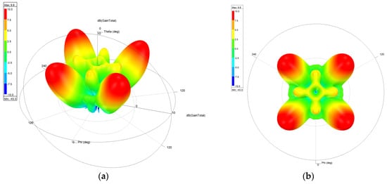
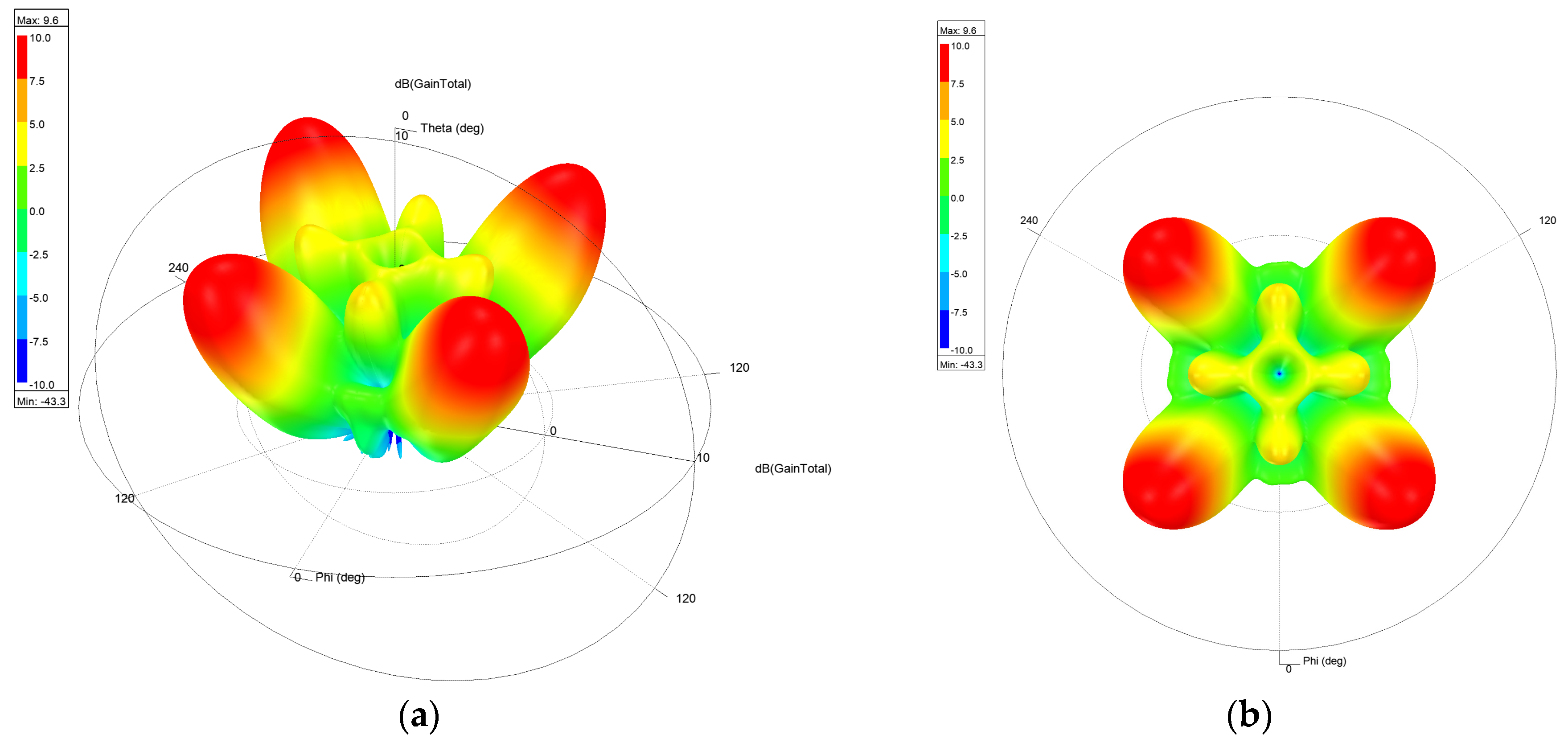
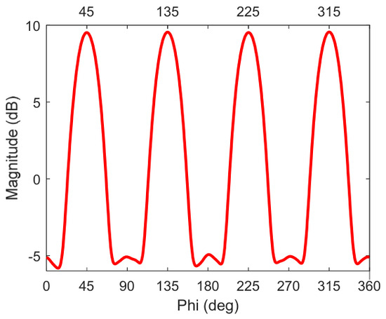
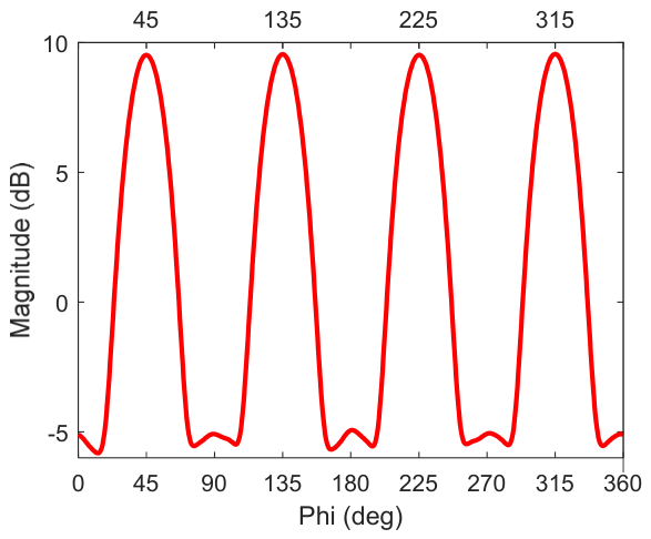
The quad-beam radiation pattern of the proposed MAS antenna is depicted in Figure 8, where Figure 8a is the 3-D view and Figure 8b is the top view. It can be observed that there are four symmetric beams in the antenna pattern. Figure 9 illustrates the 2-D antenna pattern at $\theta =45°$, which shows there are four symmetric main beams at $(\theta =45°, \varphi =45°)$, $(\theta =45°, \varphi =135°)$, $(\theta =45°, \varphi =225°)$, and $(\theta =45°, \varphi =315°)$, respectively.

Figure 8. The antenna pattern of the antenna operating at 50 GHz. (a) 3-D view; (b) top view.

Figure 9. The 2-D pattern at $\theta =45°$ of the quad-beam antenna.

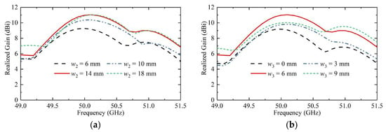
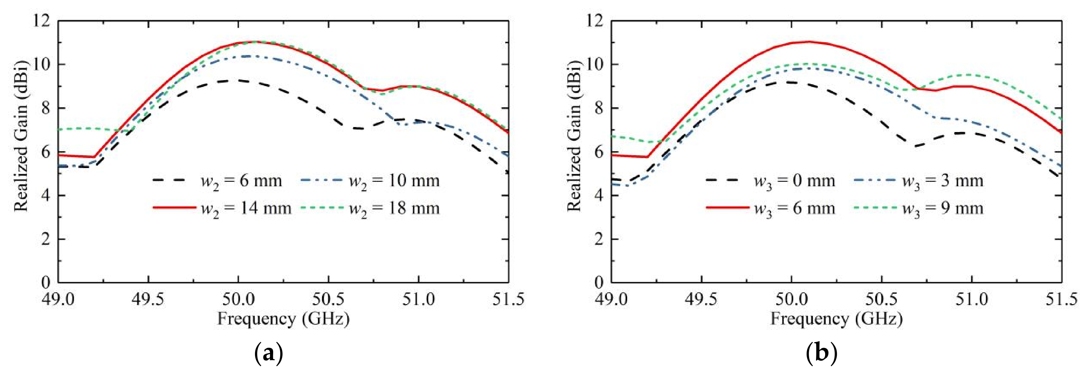
To investigate the influence of the extended dielectric substrates on the radiation performance, a parametric study was carried out. Figure 10a shows the gain variation with different extension lengths of the dielectric substrate. It can be observed that the peak gain generally increases as the extension length increases, and the maximum gain is obtained when w2 = 14 mm. Figure 10b presents the gain comparison for different extension widths. Similarly, the peak gain increases with the width of the extended dielectric substrate, and the optimal gain is achieved when w3 = 6 mm. The gain enhancement is mainly attributed to the enlarged effective radiating aperture and the improved energy concentration caused by the extended dielectric substrates. Therefore, w2 = 14 mm and w3 = 6 mm are selected as the optimized dimensions in the final design.

Figure 10. The effect of the extended dielectric substrate dimensions on the simulated antenna gain. (a) Different extension lengths. (b) Different extension widths.

3. Results

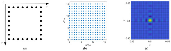
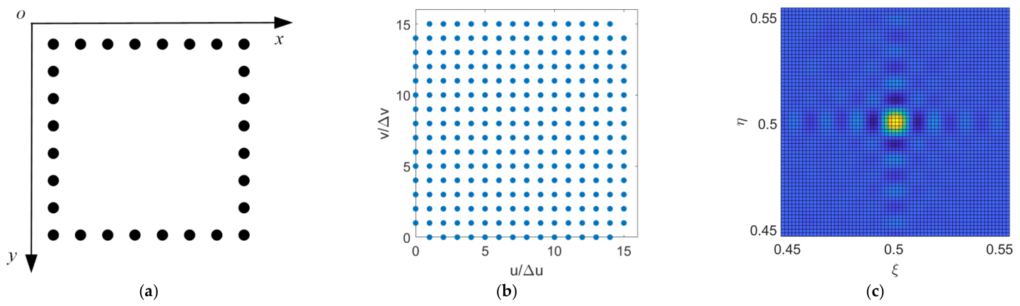
Numerical simulations are carried out to verify the feasibility of 2-D MAS radiometry based on spatial bandpass sampling and quad-beam antennas. The simulation system is the same as that used in [10,11]. The 2-D array with 28 antenna elements is arranged along the four edges of a square, with eight elements per edge, as shown in Figure 11a. The antenna spacing is 4.5 normalized with respect to the wavelength. The antenna array generates a total of 252 spatial frequency samples by 378 cross-correlations. The spatial frequency sample distribution in the uv plane is shown in Figure 11b.

Figure 11. The 2-D MAS antenna arrangement and the image reconstructed for a point source. (a) The array arrangement. (b) The spatial frequency samples in the uv plane. (c) The image reconstructed for a point source at $(\xi =0.5, \eta =0.5)$.

In the numerical simulations, the quad-beam antenna pattern in Section 2.4 is adopted, and the bandpass sampling theorem is applied to determine the sampling frequency or repetition period, and the repetition interval around $(\xi =0.5, \eta =0.5)$ is determined to be the FOV. Measurement noise due to finite integration time is also considered, and noise is added to each cross-correlation output.

For $\Delta u=4.5$ and $\Delta v=4.5$, the two repetition periods ${\xi }_s$ and ${\eta }_s$ are both 0.2222. As presented in Section 2.4, ${\xi }_H$ and ${\eta }_H$ are 0.5556. ${\xi }_L$ and ${\eta }_L$ are 0.4444. The simulated imaging region is a square region centered at (0.5, 0.5), with the four vertices at $(\xi =0.4444, \eta =0.4444)$, $(\xi =0.4444, \eta =0.5556)$, $(\xi =0.5556, \eta =0.4444)$, and $(\xi =0.5556, \eta =0.5556)$, respectively.

For a point source at $(\xi =0.5, \eta =0.5)$, the reconstructed image is shown in Figure 11c. The reconstructed BT distribution is consistent with theoretical expectation, and the Gibbs phenomenon due to truncation in the uv plane can also be observed.

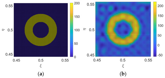
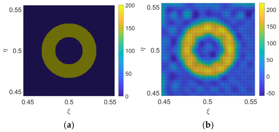
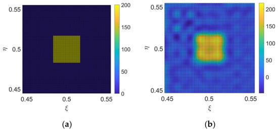
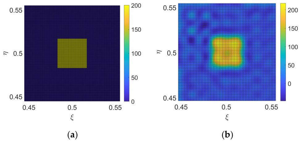
The simulation results for extended sources are shown in Figure 12 and Figure 13. For an extended source with a circular-ring-shaped BT distribution shown in Figure 12a, the reconstructed BT image is shown in Figure 12b. For an extended source with a square-shaped BT distribution in Figure 13a, the reconstructed BT image is shown in Figure 13b. Both the simulation results for the two extended sources are consistent with theoretical expectations, which verifies the feasibility of 2-D MAS based on spatial bandpass sampling and quad-beam antennas.

Figure 12. A numerical simulation for an extended source with a circular-ring-shaped brightness temperature distribution. (a) The real image; (b) the reconstructed image.

Figure 13. A numerical simulation for an extended source with a square-shaped brightness temperature distribution. (a) The real image; (b) the reconstructed image.

4. Discussion

4.1. Comparison Between Conventional MAS and the Proposed MAS

For conventional MAS, the imaging region is the neighborhood of the coordinate origin in the image plane. The reflector must be very large to receive the reflected signals from all pixels, especially those with small $\theta$ and $\varphi$ approaching 0° and 90°. But for MAS with bandpass spatial sampling and quad-beam antennas, the imaging region is restricted to an interval centered at $(\theta =45°, \varphi =45°)$, and the reflector dimensions can be greatly reduced compared with conventional MAS. As presented in Section 2.2, for a conventional MAS radiometer, the required height for the two reflectors exceeds 1000 m, whereas this value is drastically reduced to 2.205 m in the proposed scheme, making practical deployment feasible.

Bandpass spatial sampling and quad-beam antennas must be adopted. If the Nyquist baseband sampling theorem is applied for the shifted imaging region in the simulation, the FOV for baseband sampling should cover a large region with $0\le \xi \le 0.5556$ and $0\le \eta \le 0.5556$, and the corresponding normalized antenna spacing is $\Delta u=0.9$ and $\Delta v=0.9$, which are much smaller than 4.5 for the bandpass case. The antenna size for the baseband case will be greatly reduced to 1/5 of the antenna size with the bandpass case, which will result in lower antenna gain and impact the sensitivity. Furthermore, the array size for the baseband case will be greatly reduced to 1/5 of the array size with bandpass case, which will severely degrade the spatial resolution.

Conventional antennas are typically of single-beam configuration, with their main lobe pointing along the 0° angular direction. If this type of antenna beam is adopted, the shifted imaging region will lie in the low-gain direction of the antenna, which reduces the signal-to-noise ratio (SNR) of the received signals and degrade system sensitivity. The quad-beam antenna is a relatively uncommon antenna configuration, but it provides the maximum gain for the oblique imaging region, which is better matched.

4.2. The Impact of System Errors

Due to the limitations in manufacturing and machining precision, all practical array systems, such as aperture synthesis radiometers, mirror aperture synthesis radiometers, and direction finding systems based on array signal processing, are affected by various types of system errors. Generally speaking, the errors from different system components can be classified into three groups: antenna errors, receiver channel errors, and baseline errors. Antenna errors include antenna pattern phase and gain errors, antenna position errors, antenna mutual coupling, and so on. Receiver channel errors include gain errors and phase errors. Baseline errors include offset errors and the fringe-washing effect. For MAS, due to the existence of the reflectors, the nonideal reflectivity of the reflectors will cause errors, and the quad-beam antenna requires high symmetry, which will also cause errors in practice. These errors will be introduced into the cross-correlation outputs and propagate during the process of solving the cosine visibilities and image reconstruction.

Some errors, such as receiver gain and phase errors and offset errors, can be well calibrated by different calibration methods. However, other errors, such as direction-dependent antenna gain errors and antenna coupling, are difficult to calibrate and should be controlled during manufacturing. In the following, taking antenna coupling as an example, the impact of antenna coupling on the reconstructed image will be simulated.

As described in [24,25,26], the impact of antenna mutual coupling on the correlation matrix is modeled as follows:

$${\mathrm{R}}_{\mathrm{m}\mathrm{a}\mathrm{t}}^{\mathrm{e}\mathrm{r}\mathrm{r}}=\mathrm{C}{\mathrm{R}}_{mat}{\mathrm{C}}^{\mathrm{H}}$$

(17)

where $R_{mat}$ is the correlation matrix without mutual coupling, $R_{mat}^{err}$ is the correlation matrix with mutual coupling, the superscript H denotes Hermitian transpose, and $C$ is the mutual coupling matrix. For a uniform linear array, the mutual coupling matrix has finite non-zero coefficients. A banded symmetric Toeplitz matrix can be adopted to model the coefficients in the mutual coupling matrix as follows [24,25]:

$$\mathrm{C}=\left[\begin{array}{cccccc}1& c_1& \cdots & c_{L-1}& \cdots & 0\\ c_1& 1& c_1& \cdots & \ddots & ⋮\\ ⋮& c_1& 1& c_1& \cdots & c_{L-1}\\ c_{L-1}& \cdots & \ddots & \ddots & \ddots & ⋮\\ ⋮& ⋮& \ddots & c_1& 1& c_1\\ 0& \cdots & c_{L-1}& \cdots & c_1& 1\end{array}\right]$$

(18)

with $0<\left|c_1\right|,\left|c_2\right|,\dots ,\left|c_{L-1}\right|<1$.

In addition, the coefficients can be modeled by an exponential attenuation according to the spacing between the two antennas.

For the 2-D array arranged as a rectangular shape in the numerical simulation, it can be regarded as a long uniform linear array with a closed loop. Therefore the coefficients for the mutual coupling for the 2-D array can adopt the form in (18). The minimum antenna spacing in the simulation is $4.5\lambda ,$ which is large enough, and the mutual coupling is assumed to be negligible for antenna spacing greater than $3\ast 4.5\lambda$. Hence, $L=3$ is set in (18). In the simulation, the magnitude of $c_1$ is set to 0.1 (−10dB level) and 0.025 (−16dB level), respectively. The magnitude of $c_2$ is set to be a quarter of $c_1$. The reconstructed BT image impacted by mutual coupling will be compared with the ideal reconstructed BT image. And the root mean square error can be calculated to evaluate the impact:

$$RMSE=\sqrt{{\displaystyle \frac{1}{MN}}{\displaystyle \sum _{m=1}^M}{\displaystyle \sum _{n=1}^N}{{(T}_{err}({\xi }_m, {\eta }_n)-T({\xi }_m, {\eta }_n))}^2}$$

(19)

where $T_{err}({\xi }_m, {\eta }_n)$ is the reconstructed BT with errors, and $T({\xi }_m, {\eta }_n)$ is the reconstructed BT without errors.

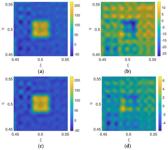
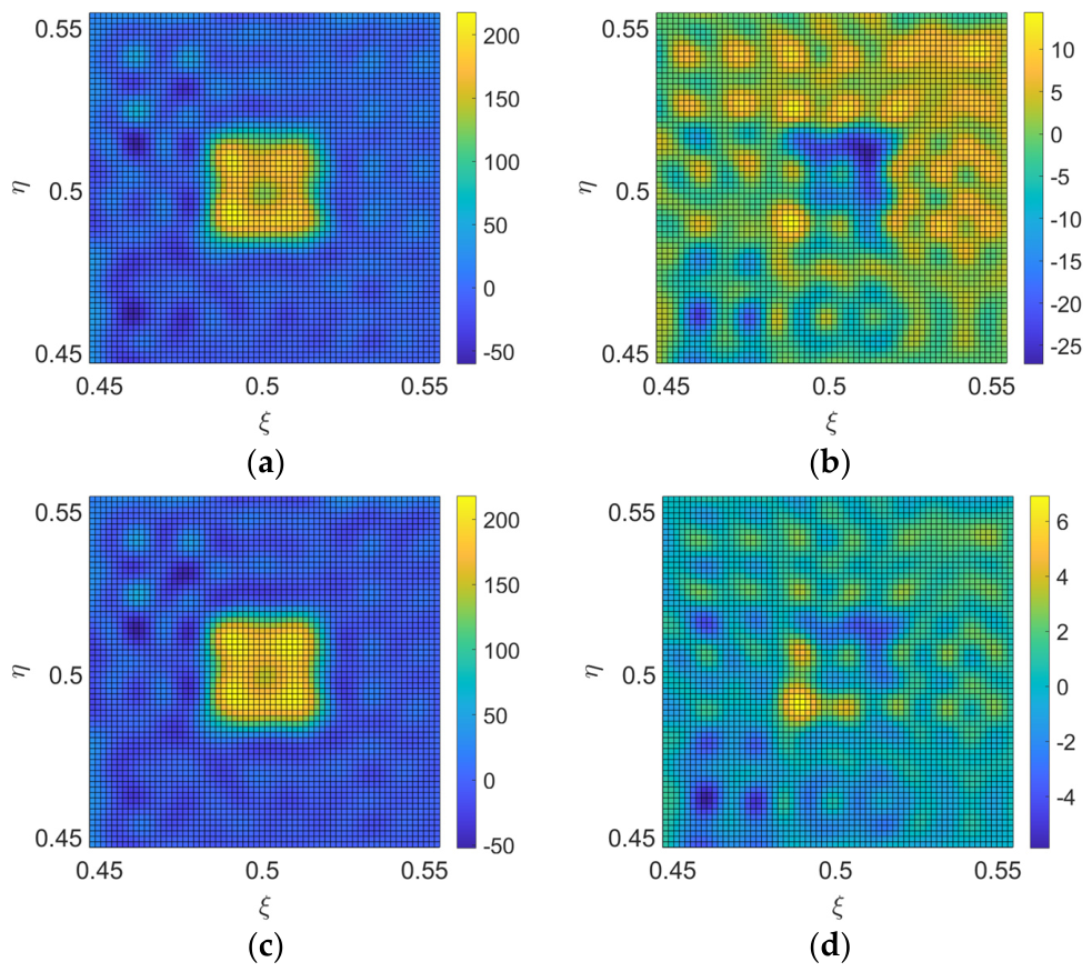
When $c_1=0.1e^{i\ast \pi /6}$ and $c_2=0.025e^{i\ast \pi /3}$ are set, for the square-shaped BT distribution in Figure 13a, the reconstructed image with errors is illustrated in Figure 14a. Figure 14b is the error image between Figure 14a and Figure 13b. The RMSE is 6.07 K, which is large and cannot be accepted.

Figure 14. The reconstructed BT image with the impact of antenna mutual coupling. (a) The reconstructed BT image with $c_1=0.1e^{i\ast \pi /6}$ and $c_2=0.025e^{i\ast \pi /3}$; (b) the error image between (a) and Figure 13b; (c) the reconstructed BT image with $c_1=0.025e^{i\ast \pi /6}$ and $c_2=0.00625e^{i\ast \pi /3}$; (d) the error image between (c) and Figure 13b.

When $c_1=0.025e^{i\ast \pi /6}$ and $c_2=0.00625e^{i\ast \pi /3}$ are set, the reconstructed image with errors is illustrated in Figure 14c. Figure 14d is the error image between Figure 14c and Figure 13b. The RMSE is 1.44 K. Therefore, the mutual coupling must be controlled to a suitable level to guarantee the accuracy of the reconstructed BT image.

Only theoretical analysis and numerical simulations are applied to demonstrate the validity. Prototype imaging experiments are necessary to further demonstrate the method in future. In addition, performance evaluations are derived only from simulation data, which cannot fully cover various system errors in actual engineering implementation.

5. Conclusions

To reduce the dimensions of the two reflectors in 2-D MAS, the center of the image region is shifted from the incident angle of 0° to the oblique direction of $(\theta =45°, \varphi =45°)$, the results of which are quite different from conventional aperture synthesis. MAS radiometry based on spatial bandpass sampling and quad-beam antennas is proposed to match the shift. To maximize the antenna spacing and enlarge the array size, the bandpass sampling theorem is applied to sample the spatial bandpass signal. The relationship between the antenna spacing and the boundary of the imaging region is discussed. Furthermore, quad-beam antennas are proposed and designed for this specific case. Numerical simulations for the point source BT distribution and extended BT distribution demonstrate the feasibility of the proposed method.

Although the reflector dimension issue is addressed, this method imposes higher requirements on antenna design and manufacture, especially in terms of beam symmetry and pattern consistency among antenna elements.

References

- McMullan, K.D.; Brown, M.A.; Martin-Neira, M.; Rits, W.; Ekholm, S.; Marti, J.; Lemanczyk, J. SMOS: The Payload. IEEE Trans. Geosci. Remote Sens. 2008, 46, 594–605. [Google Scholar] [CrossRef] [Scilit]
- Boutin, J.; Martin, N.; Yin, X.; Font, J.; Reul, N.; Spurgeon, P. First assessment of SMOS data over open ocean: Part II—Sea surface salinity. IEEE Trans. Geosci. Remote Sens. 2012, 50, 1662–1675. [Google Scholar] [CrossRef] [Scilit]
- Li, Y.; Yin, X.; Zhou, W.; Lin, M.; Liu, H.; Li, Y. Performance simulation of the payload IMR and MICAP onboard the Chinese ocean salinity satellite. IEEE Trans. Geosci. Remote Sens. 2021, 60, 5301916. [Google Scholar]
- Yin, X.; Boutin, J.; Spurgeon, P. First assessment of SMOS data over open ocean: Part I—Pacific Ocean. IEEE Trans. Geosci. Remote Sens. 2012, 50, 1648–1661. [Google Scholar] [CrossRef]
- He, L.; Huang, S.; Hui, F.; Cheng, X. An improved algorithm for retrieving thin sea ice thickness in the Arctic Ocean from SMOS and SMAP L-band radiometer data. Acta Oceanol. Sin. 2024, 43, 127–138. [Google Scholar] [CrossRef] [Scilit]
- Rodriguez-Fernandez, N.J.; Anterrieu, E.; Cabot, F.; Boutin, J.; Picard, G.; Pellarin, T.; Merlin, O.; Vialard, J.; Vivier, F.; Costeraste, J.; et al. A New L-Band Passive Radiometer For Earth Observation: SMOS-High Resolution (SMOS-HR). In Proceedings of the IGARSS 2020—2020 IEEE International Geoscience and Remote Sensing Symposium, Waikoloa, HI, USA, 26 September–2 October 2020; pp. 5978–5981. [Google Scholar]
- Tanner, A.B.; Wilson, W.J.; Lambrigsten, B.H.; Dinardo, S.J.; Brown, S.T.; Kangaslahti, P.P.; Gaier, T.C.; Ruf, C.S.; Gross, S.M.; Lim, B.H.; et al. Initial Results of the Geostationary Synthetic Thinned Array Radiometer (GeoSTAR) Demonstrator Instrument. IEEE Trans. Geosci. Remote Sens. 2007, 45, 1947–1957. [Google Scholar] [CrossRef] [Scilit]
- Christensen, J.; Carlström, A.; Emrich, A.; de Maagt, P. The Geostationary Atmospheric Sounder (GAS); SPIE: Bellingham, WA, USA, 2006; Volume 6361. [Google Scholar]
- Liu, H.; Niu, L.; Zhang, C.; Han, D.; Lu, H.; Zhao, X.; Wu, J. Preliminary results of GIMS-II (Geostationary interferometric microwave sounder-second generation) demonstrator. In Proceedings of the 2017 IEEE International Geoscience and Remote Sensing Symposium (IGARSS), Fort Worth, TX, USA, 23–28 July 2017; pp. 711–714. [Google Scholar]
- Chen, L.; Li, Q.; Yi, G.; Zhu, Y. One-Dimensional Mirrored Interferometric Aperture Synthesis: Performances, Simulation, and Experiments. IEEE Trans. Geosci. Remote Sens. 2013, 51, 2960–2968. [Google Scholar] [CrossRef] [Scilit]
- Dou, H.; Gui, L.; Li, Q.; Chen, L.; Bi, X.; Wu, Y.; Lei, Z.; Li, Y.; Chen, K.; Lang, L. Initial results of microwave radiometric imaging with mirrored aperture synthesis. IEEE Trans. Geosci. Remote Sens. 2019, 57, 8105–8117. [Google Scholar] [CrossRef]
- Lei, Z.; Chen, K.; Li, Q.; Dou, H.; Xiao, C. Rank-Full Arrays for 1-D Mirrored Aperture Synthesis. IEEE Geosci. Remote Sens. Lett. 2022, 19, 8009105. [Google Scholar] [CrossRef] [Scilit]
- Wu, R.; Xiao, C.; Lei, Z.; Dong, J.; Zhang, Y. 1-D Mirrored Aperture Synthesis Based on Artificial Magnetic Conductor. IEEE Geosci. Remote Sens. Lett. 2025, 22, 4501205. [Google Scholar] [CrossRef] [Scilit]
- Zhu, D.; Hu, F.; Wu, L.; Li, J.; Lang, L. Low-redundancy linear arrays in mirrored interferometric aperture synthesis. Opt. Lett. 2016, 41, 368–371. [Google Scholar] [CrossRef] [Scilit] [PubMed]
- Li, H.; Li, G.; Dou, H.; Xiao, C.; Lei, Z.; Lv, R.; Li, Y.; Wu, Y.; Song, G. Array Configuration Design for Mirrored Aperture Synthesis Radiometers Based on Dual-Polarization Measurements. Remote Sens. 2022, 15, 167. [Google Scholar] [CrossRef] [Scilit]
- Li, Y.; Li, Q.; Feng, L. Relationship between mirrored aperture synthesis radiometers and aperture synthesis radiometers. IEEE Geosci. Remote Sens. Lett. 2017, 14, 631–635. [Google Scholar] [CrossRef] [Scilit]
- Li, Y.; Li, Q.; Gui, L.; Feng, L.; Dou, H.; Lei, Z. Image reconstruction for mirrored aperture synthesis radiometers. IEEE Trans. Geosci. Remote Sens. 2020, 58, 7720–7733. [Google Scholar] [CrossRef] [Scilit]
- Xiao, C.; Li, Q.; Zhao, G.; Huang, Y. Brightness temperature image reconstruction of the tilted mirrored aperture synthesis using CNN and transformer. IEEE Trans. Geosci. Remote Sens. 2024, 62, 5208116. [Google Scholar] [CrossRef] [Scilit]
- Li, Y.; Li, Q.; Feng, L. Analysis of reflector sizes in rotating mirrored aperture synthesis radiometers. IEEE Geosci. Remote Sens. Lett. 2018, 15, 907–911. [Google Scholar] [CrossRef] [Scilit]
- Chen, L.; Tian, Y.; Zhao, L.; Li, Q.; Lei, Z.; Jin, R. The Impact of Antenna Polarization on Mirrored Aperture Synthesis Radiometry. IEEE Trans. Geosci. Remote Sens. 2026, 64, 5301015. [Google Scholar] [CrossRef] [Scilit]
- Oppenheim, A.V.; Willsky, A.S.; Nawab, S.H. Signals & Systems; Pearson Education: London, UK, 1997. [Google Scholar]
- Pozar, D.M. Microwave Engineering; John Wiley & Sons: Hoboken, NJ, USA, 2011. [Google Scholar]
- Xu, F.; Wu, K. Guided-wave and leakage characteristics of substrate integrated waveguide. IEEE Trans. Microw. Theory Tech. 2005, 53, 66–73. [Google Scholar] [CrossRef] [Scilit]
- Wang, Y.; Trinkle, M.; Ng, B.W.-H. DOA Estimation under Unknown Mutual Coupling and Multipath with Improved Effective Array Aperture. Sensors 2015, 15, 30856–30869. [Google Scholar] [CrossRef] [Scilit] [PubMed]
- Ye, Z.; Dai, J.; Xu, X.; Wu, X. DOA Estimation for Uniform Linear Array with Mutual Coupling. IEEE Trans. Aerosp. Electron. Syst. 2009, 45, 280–288. [Google Scholar] [CrossRef] [Scilit]
- Dai, J.; Xu, W.; Zhao, D. Real-valued DOA estimation for uniform linear array with unknown mutual coupling. Signal Process. 2012, 92, 2056–2065. [Google Scholar] [CrossRef] [Scilit]
Disclaimer/Publisher’s Note: The statements, opinions and data contained in all publications are solely those of the individual author(s) and contributor(s) and not of MDPI and/or the editor(s). MDPI and/or the editor(s) disclaim responsibility for any injury to people or property resulting from any ideas, methods, instructions or products referred to in the content. |
© 2026 by the authors. Licensee MDPI, Basel, Switzerland. This article is an open access article distributed under the terms and conditions of the Creative Commons Attribution (CC BY) license.