Satellite Detection of Diffuse Tectonic CO₂ Degassing in the East African Rift

Highlights

What are the main findings?

• The statistical decomposition of long-term satellite-derived column CO₂ time series shows that diffuse surface degassing can be detected from space over large regions without ancillary ground measurements or atmospheric models.
• Applied to the East African Rift region, this approach reveals a coherent spatial pattern of CO₂ fluxes associated with major fault systems and extending into plateau areas where magmatism ceased millions of years ago.

What are the implications of the main findings?

• These results indicate that satellite-based column CO₂ measurements, when analysed with a statistical deconvolution of the column signal, retain resolvable information about extended surface fluxes that would otherwise be masked by the atmospheric transport and mixing processes.
• This study highlights the potential of a statistical analysis of spaceborne CO₂ observations as a robust framework for identifying and mapping diffuse tectonic degassing at large spatial scales. Although further calibration is required to constrain magnitudes of absolute fluxes, the approach provides new opportunities to identify natural carbon emissions and link satellite observations to solid-Earth processes.

Abstract

Understanding the processes behind Earth’s CO₂ degassing is crucial for clarifying how carbon is cycled by geologic processes on our planet. Earth’s carbon degassing results from magmatic and metamorphic processes controlled by large-scale plate tectonics. However, the nature and amount of diffuse CO₂ fluxes from faults in continental rifts remain largely unconstrained. Recent research reports important CO₂ fluxes from deep faults over 17 × 10⁴ km² in the East African Rift System (EARS), highlighting the need for a more detailed inventory of diffuse soil emissions. Across such extensive regions, only satellite observations can provide the broad measurement range needed to meet the observational requirements for long-term, large-scale overlay datasets. While space-based data provide extended coverage for large-scale identification of CO₂ emission sources, to date, only the column-averaged total CO₂ atmospheric content has been measured from space. Range-resolved measurements of CO₂ concentration with the vertical accuracy needed to detect diffuse soil emissions are not available from space, preventing direct quantification of Earth degassing over large regions. In this paper, we focus on a new approach to measuring soil CO₂ fluxes by a statistical deconvolution of column measurements of global atmospheric CO₂ content. Anthropogenic increase, seasonal climatology at a small regional scale, and soil fluxes are measured without the use of ancillary measurements or model simulations. We combine petrology of fluid and melt phases in mantle rocks with a new satellite data analysis to reveal, for the first time, large CO₂ fluxes from the lithospheric mantle to the atmosphere in a much wider region than previously considered (22.4 × 10⁵ km²), including the Ethiopian and East African domes, where magmatism is no longer active or absent. We infer that diffuse soil emissions are measurable from space, and that Earth’s tectonic carbon fluxes are considerably more relevant than currently considered, with a crucial impact on the balance of the global carbon cycle.

1. Introduction

The global increase in atmospheric CO₂, mainly attributed to anthropogenic sources and to point-like natural emissions from wildfires and volcanic degassing, has been assessed using a variety of ground-based measurements, space-based monitoring, and atmospheric models.

International networks for ground-based measurements of atmospheric CO₂ content have been established to harmonise global CO₂ time series and to calibrate satellite-measured column-average CO₂ content, improving estimates of CO₂ sources and sinks [1,2,3,4,5,6,7,8]. Moreover, past and present Space-Based CO₂ observations have assessed the total column atmospheric content with different accuracies, footprints and observational strategies. Dedicated CO₂ spaceborne measurements have been designed for high-precision global atmospheric CO₂ measurements, some focusing on urban emissions and regional fluxes and others on global CO₂ concentration. Moreover, non-dedicated satellite missions are designed for broader atmospheric chemistry monitoring, including CO₂ retrievals among other atmospheric measurements [9,10,11,12,13,14,15,16]. Future missions are designed to globally monitor anthropogenic CO₂ emissions through a dedicated satellite constellation and to support climate policy and improve attribution of emission sources [17,18].

Spaceborne measurements of column-averaged XCO₂ are used in conjunction with measurements of other atmospheric parameters and models to identify CO₂ sources, the spatiotemporal variation in atmospheric CO₂ content, and CO₂ fluctuations associated with seasonal climatology at regional and global scales. A variety of methods, such as Atmospheric Transport Modelling, Bayesian Inverse Modelling, Plume Detection and Mass Balance Methods, Averaging Kernels and Sensitivity Analysis, have been implemented to resolve the mixing of ground CO₂ emissions in the total column atmospheric concentration [19,20,21,22,23,24,25].

Retrieval algorithms used to derive XCO2 L2 data from radiance spectra rely on prior knowledge and statistical weighting from models, limiting independent vertical information and potentially introducing bias near the surface. A priori information is essential, though the degree and role of the prior differ among methods. In the solar absorption measurements, the satellite spectral measurement from which the synthetic column-averaged XCO₂ is retrieved shows broad sensitivity throughout the troposphere but provides only limited information on CO₂ within the boundary layer. In the Bayesian (optimal-estimation) retrieval, this limited near-surface sensitivity increases reliance on the a priori profile and forces the solution to lean on the prior in the lowest layers, smoothing sharp vertical gradients and causing real surface enhancements to appear strongly attenuated in XCO₂ variations [26,27,28]. In thermal infrared sounder retrievals that simultaneously estimate temperature, water vapour, and CO₂, the optical thickness of the lower atmosphere limits the sensitivity to the boundary-layer concentrations. CO₂ emitted near the surface is not directly observed and becomes detectable only after vertical mixing transports it into free-tropospheric layers to which the instrument is sensitive [29,30,31]. Despite extensive international efforts, satellite observations can reliably detect and quantify certain ground-based CO₂ emission sources, but not all sources and not under all conditions. Their effectiveness depends on factors such as source magnitude, atmospheric conditions, instrument characteristics, and the analytical methods applied. Consequently, in situ measurements and emission inventories remain essential for identifying and quantifying ground-based emission sources [32,33,34,35]. In particular, distinguishing natural emission sources from the atmospheric background is difficult because their output is minimal compared to the background and requires favourable wind geometry and satellite overpasses above the unknown point-like sources. Extremely high-sensitivity spaceborne measurements have been used to identify volcanic plumes, detecting the spatial variability of column CO₂ measurements at kilometre-scale resolution at the ground, jointly with the measured wind field [36]. However, to date, spaceborne observations of natural CO₂ sources have remained relatively limited, with only a few studies reporting the detection or quantification of volcanic CO₂ emissions, particularly during major eruptive events [37,38,39].

In continental rift settings, CO₂ emissions are not restricted to localised volcanic vents but may occur as diffuse degassing along crustal- and lithospheric-scale fault systems [40,41,42]. Ground-based studies in the East African Rift have documented mantle-derived CO₂ emissions distributed over tens to hundreds of kilometres [43,44], indicating that degassing may affect broad tectonic provinces rather than isolated point sources. Such spatially distributed emissions cannot be adequately characterised by local measurements alone. However, to date, range-resolved measurements of CO₂ concentration with the vertical accuracy needed to detect diffuse soil emissions over large areas are not available from space. Satellite measurements of soil degassing have not been reported, preventing direct quantification of diffuse CO₂ soil degassing over large regions and its influence on the total carbon budget.

In this paper, we focus on a new approach to measuring soil CO₂ sources by statistical deconvolution of area-averaged time-series column measurements of global atmospheric CO₂ content, which is well mixed by atmospheric transport.

Anthropogenic increase, seasonal climatology at a small regional scale, and soil fluxes are assessed without the use of ancillary measurements or model simulations. The resolution of the three main components of the column-averaged CO₂ atmospheric content reveals new physical phenomena and unexpected CO₂ sources. We test this approach across East Africa, a region characterised by active continental rifting and documented mantle-derived CO₂ emissions; it is also well-suited for large-scale, long-term characterisation of diffuse soil emissions [43,44,45,46,47,48,49]. Geological and petrological evidence indicates that the infiltration of carbonate–silicate melts into the subcontinental lithospheric mantle generates significant CO₂ at depth [50,51,52,53]. However, whether any part of this deep carbon reservoir contributes to diffuse surface degassing over large spatial scales remains unresolved. While additional calibration is required to improve estimates of absolute fluxes, this approach offers promising opportunities to quantify natural carbon emissions at regional to continental scales and to better integrate satellite data with solid-Earth processes.

By integrating satellite statistical signal decomposition with independent geological constraints, we assess whether diffuse tectonic CO₂ emissions can be detected from space.

2. Materials and Methods

2.1. R-Decomposition of Row Satellite Data and Time Series Statistical Analysis

We used a statistical decomposition of the area-averaged column signal from the Atmospheric Infrared Sounder (AIRS) on board the NASA/AQUA satellite (https://airs.jpl.nasa.gov) [15] to deconvolve the total CO₂ column measurement content into three components: the long-term evolution of the total atmospheric content, the seasonal variations, and the residuals. We used an observed discrete time series set of 114 paired values ${\{t_k,x_k\}}_{k=1}^{114}$, where $t_k$ is the time equally sampled in months, from September 2002 to February 2012, and $x_k$ is the corresponding area-averaged column concentration of carbon dioxide, measured in ppm from satellite in grid boxes of 1.66° × 1.66°. The time series are decomposed into three additive components using a decomposition function in R [54]:

$$x_i=x_{trend,i}+x_{seasonal,i}+x_{residual,i}$$

(1)

where the trend component $x_{trend,i}$ is calculated as a 12-month moving average. This cannot be calculated for the first 6 and the last 6 paired values, reducing the statistical set to 102 values. The seasonal component $x_{seasonal,i}$ is calculated as the monthly mean after subtraction of the trend component from the signal, and the residuals component $x_{residual,i}$ is calculated as the difference between the measured time series and the sum of the trend and the seasonal components.

$$x_{residual,i}=x_i-(x_{trend,i}+x_{seasonal,i})$$

(2)

The statistical properties, in particular, the stationarity of the residual components, have been assessed using the ADF (Augmented Dickey–Fuller) Test and the KPSS Test for Level Stationarity [55,56,57].

2.2. AIRS/AQUA Observations of Column CO₂

The approach proposed in the paper uses the carbon dioxide mole fraction X_CO2 data in the free troposphere retrieved from AIRS on board the NASA/AQUA satellite (https://airs.jpl.nasa.gov). AIRS was launched in May 2002 in a sun-synchronous 705 km polar orbit, providing 95% global daily coverage in 15 orbits and a scanning pattern that creates two swaths per day. At the North Pole, total coverage is assured by the overlapping of swaths; gaps arise at the equator. We chose to use AIRS data based on comparative studies of the accuracy of CO₂ concentration retrievals from different satellite products. Results have shown excellent agreement between the AIRS data and ground-based measurements, thereby demonstrating the ability of AIRS products to represent the true distribution and changes in CO₂ with the best coverage and accuracy, making them particularly suitable for our purposes [30,57]. For CO₂ monitoring of Earth degassing in Ethiopia, thermal infrared observations from AIRS provide a valuable dataset, enabling a long-term trend analysis due to its continuous record, day–night capability, and reduced sensitivity to cloud cover in convective tropical conditions. The AIRS retrieval system jointly retrieves a set of atmospheric and surface variables, including atmospheric temperature and water-vapour profiles, ozone, cloud properties, surface skin temperature, and surface spectral emissivity. These jointly retrieved quantities provide a physically consistent characterisation of the atmospheric and surface state and allow the effects of interfering atmospheric and surface variables to be accounted for within the retrieval process. The resulting Level-2 retrievals undergo calibration, quality control, and assessment of retrieval errors before being aggregated into the Level-3 gridded products used in this study.

The AIRS CO₂ retrievals demonstrated the ability to reproduce the variability measured in flask observations, with an accuracy of 0.43 ± 1.20 ppm [58]. For a statistical ensemble of 102 independent time-series samples, the uncertainty of the mean is reduced to 0.12 ppm, corresponding to a variance of 0.014 ppm² in each grid cell.

AIRS primarily senses mid-tropospheric CO₂. In Ethiopia, where strong daytime convection promotes vertical mixing, mid-tropospheric CO₂ often reflects broader atmospheric conditions influencing the total column. This layer, where vertical mixing is frequent, reflects regional atmospheric transport and long-term background variability, making the dataset well-suited for long-term trend analysis and statistical deconvolution of total column content. In contrast, solar-reflectance missions such as OCO-2 provide high-precision column measurements but rely on clear-sky conditions and may exhibit sampling limitations in convective tropical regions. Consequently, AIRS provides a stable, temporally consistent dataset for assessing long-term variability and regional atmospheric dynamics, complementing higher-precision column measurements that may be more spatially intermittent and are then better suited to deconvolving total column measurements.

Data: We used level 3 data, version 6, monthly-averaged over 1.66° × 1.66° areas, freely available from NASA Earthdata, including means and standard deviations calculated from all 15 orbits and averaged into daily, eight-day, and monthly Gridded Retrieval ProductsThe mean values are calculated as the arithmetic means of the individual CO₂ measurements within each grid box and are therefore well-suited for the direct identification of different CO₂ components. The use of level 3 data from AIRS/AQUA prevents contamination of the deconvolution of CO₂ column measurements into their three components by instrumental noise, ensuring the physical interpretation of the results.

Data validation information is available at https://airs.jpl.nasa.gov/data/validation/ accessed on 10 June 2026.

Data availability and retrieval: NASA supports free and open use of data for research and applications (https://earthdata.nasa.gov/collaborate/open-data-services-and-software accessed on 10 June 2026). AIRS global 1.66° × 1.66° Level-3 Products were retrieved using the Geospatial Interactive Online Visualization ANd aNalysis Infrastructure, Giovanni [59] (https://giovanni.gsfc.nasa.gov/giovanni/ accessed on 10 June 2026).

2.3. Raman Microspectroscopy

Microstructural and chemical in situ analysis of fluid and mineral phases was performed using Raman spectroscopy with a Horiba Jobin Yvon (France) LabRAM HR Evolution spectrometer, an 800 mm focal length, a 1024 px CCD detector, and two diffraction gratings (1800 and 600 g/mm). The Nd 532.06 nm laser source at 300 mW power has a wheel of nine neutral-density filters to attenuate the intensity. Analyses were carried out at the Department of Earth and Environmental Sciences, University of Milano-Bicocca. Fifteen double-polished mantle rock sections, approximately 100–150 µm thick, were prepared for petrological investigations. Analysis of fluid inclusions was performed down to a depth of 20 µm below the sample surface using a transmitted-light Olympus B40 microscope. A 100 × objective (Numerical aperture, N.A., =0.90) with a long-working distance was used for all the acquisitions to increase spatial resolution (<1 µm). The spectrometer was calibrated over the 0–1500 cm⁻¹ region using a silicon standard and a natural diamond standard at the beginning of each Raman session. Spectra were collected with a laser power of 50 mW, for variable acquisition times (from 5 to 60 s) and 1 to 3 acquisitions to obtain the best signal-to-noise ratio. A band central position accuracy of 1.2 cm⁻¹ was obtained by combining a 600 g/mm diffraction grating. Spectra were baseline-corrected and processed using statistical analysis [60]. The line shape of the entire spectrum was deconvoluted into single-band profiles using a Voigt pseudo-function, which is a convolution of a Lorentzian and a Gaussian line shape. In this way, the central position of the bands was determined with an accuracy of better than 0.2 cm⁻¹. The assignment of Raman peaks was performed by comparison with our spectral database [61].

3. Results

3.1. Statistical Analysis: Physical Interpretation of the Result CO₂ Profile

The deconvolution of the total column content as measured by the satellite shows three large-scale, long-term components: the bulk atmospheric content, the cycling respiration, and a third component, the residuals, all mixed by atmospheric circulation. Statistical analysis has shown that the signal dataset, as well as the anthropogenic and vegetation cyclic respiration, strongly represent non-stationary and non-ergodic processes, reflecting well the non-stationary character of the total CO₂ column increase and the vegetation cycle. In contrast, in-depth analysis has revealed that the residual statistical dataset is stationary and ergodic, precluding its interpretation as the remaining statistical fluctuations of the other components of the signal. The statistical properties, and, in particular, the stationarity of the residual components, have been assessed using the ADF (Augmented Dickey–Fuller) Test and KPSS Test for Level Stationarity, and by calculating the mean,

$$\overline{x}={\displaystyle \frac{1}{n}}{\displaystyle \sum _{i=1}^n{x}_{residual,i}}$$

(3)

the variance,

$$V(x_{residual})={\displaystyle \frac{1}{n-1}}{\displaystyle \sum _{i=1}^n(x_{residual,i}}-\overline{x}{)}^2$$

(4)

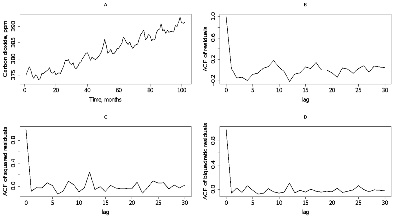
and the autocorrelation function of the corresponding statistical ensembles in the different grid boxes [54,55,56]. Results show that the mean and variance of the residuals are largely constant across statistically complete or partially sampled time intervals. Confirming the stationarity of the residuals, the autocorrelation function between the residual’s values $x_{residual,i}$ and $x_{residual,j}$ in the same grid box, calculated for different statistical complete or partial sampled time intervals $[t_j;t_{j+(n-1)}]$, appears to only be a function of the lag. The ergodicity of the residual components is further assessed by the vanishing of the autocorrelation functions of the higher moments of their statistical distribution, e.g., the autocorrelation function for the squared residuals $x_{residual,i}^2$ and the autocorrelation function for the biquadratic of residuals $x_{residual,i}^4$ as a function of the lag. Slutski’s theorem, therefore, allows us to calculate the mean and the variance of the residuals using only one profile of data per grid box [62,63]. The results in Figure 1 confirm the rapid decay of the autocorrelation functions for lags greater than 1, indicating mutual independence of the data within the statistical ensemble of residuals and clearly confirming the wide-sense stationarity and ergodicity of the underlying processes.

Moreover, the residuals show different amplitudes across grid boxes that are unrelated to the amplitude of the level 3 signal measured by the satellite, and they cannot be attributed to instrumental noise. Instead, because of their statistical and physical properties, the residuals represent additional physical processes at time and area scales that are independent of the surface and atmospheric cycles. This interpretation is enhanced by a comparative analysis of trends, seasonal oscillations, and residual components across different grid boxes.

In the present analysis, decomposition of the original time series yields an ensemble of (N = 102) residues values in each grid cell. The statistical analyses described above show that these residuals are stationary and ergodic, with no significant temporal autocorrelation. Accordingly, they can be treated, for the purpose of estimating the uncertainty of the ensemble mean, as effectively independent realisations of the underlying stationary processes. Our analysis shows that the variance of the residues therefore ranges from 0.3 to 1.2 ppm², more than 20 times larger than the variance associated with the AIRS retrieval uncertainty after averaging over 102 independent time-series samples (0.014 ppm²). The uncertainty in the variance estimates is consistently below 20%.

Different statistical sets can be evaluated and selected for different geographic areas, atmospheric conditions, and geographic/geological settings to ensure the same level of accuracy. Sampling analysis performed using a 1° × 1° instead of 1.66° × 1.66° grid box has shown an equivalent pattern, indicating that the results are independent of residual atmospheric effects limited to the grid box area. This indicates the absence of correlated structures among the residues produced by diffusion degassing from independent sources.

3.2. Comparison of Trends, Seasonal and Residual Components

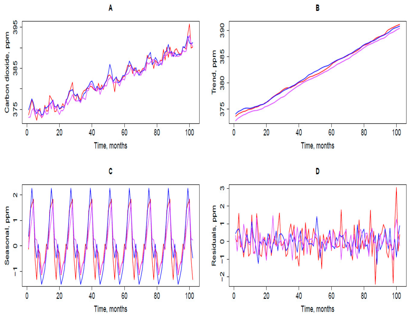
Figure 2 shows the deconvolution of the three signal components as a function of time for each grid box. In Figure 2B, the trends show roughly equal slopes in each grid box, with a maximum reciprocal variation of about 0.4% and 1% with respect to the reference Keeling curve [64]. Moreover, this is consistent with the temporal and spatial variations in annual CO₂ growth rates (AGRs) from the Total Carbon Column Observing Network (TCCON) [5], models, and satellite observations [65]. For the same grid boxes, Figure 2C reports the quasi-synchronous behaviours of the seasonal components representing the seasonal time-synchronous vegetation cycle [66]. Results show slight variations with moderate spatial variability in neighbouring areas, driven by seasonal absorption–emission differences across diverse land and vegetation cover within neighbouring grid boxes [67,68,69,70]. The terrestrial ecosystem, in terms of the CO₂ atmospheric concentration and the carbon cycle, is dominated by the time-synchronous respiration of vegetation. Strong seasonal amplitude and spatial variations at larger scales arise from differences in emission/absorption rates among diverse land and soil covers, temperature, soil humidity, and soil microbial communities [66,67,68,69]. Results in Figure 2C highlight a reciprocal variation in amplitude of about 25% in the seasonal emission–absorption rate, well representing the crucial role of the tropics in the spatial inhomogeneities of the AGR [70,71].

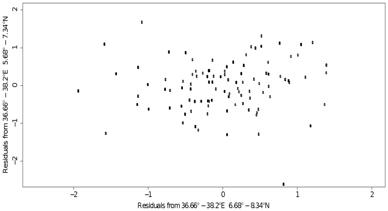
Contrary to the trend and seasonal components, the residuals reported in panel 2d correspond to time- and area-independent physical processes, showing random behaviours in each grid box, without any time or spatial synchronisation, in both amplitude and frequency. The independence of the residuals from the other two components has been confirmed by a correlation analysis. Results for the grid box 36.66–38.2°E 6.68–8.34°N are reported in

Table 1. Linear correlation coefficients: panel (a) Linear correlation coefficient of the seasonal components between the grid box (36.66–38.2°E; 6.68–8.34°N) and its adjoining areas; panel (b) Linear correlation coefficient of the residuals components between the grid box (36.66–38.2°E; 6.68–8.34°N) and its adjoining areas.

Panel (a) Seasonal Components	36.66–38.2°E; 6.68–8.34°N
36.66–38.2°E; 8.34–10°N	0.9350112
35–36.66°E; 6.68–8.34°N	0.6512518
36.66–38.2°E; 5.68–7.34°N	0.8783526
38.2–39.8°E; 6.68–8.34°N	0.7882966
Panel (b) Residuals	36.66–38.2°E; 6.68–8.34°N
36.66–38.2°E; 8.34–10°N	0.2603765
35–36.66°E; 6.68–8.34°N	0.1302511
36.66–38.2°E; 5.68–7.34°N	0.09333776
38.2–39.8°E; 6.68–8.34°N	0.2655219

and Figure 3, as an example. The seasonal components show linear correlation coefficients ranging from 0.65 to 0.93. In contrast, the values between residuals in neighbouring grid boxes are small, ranging from 0.09 to 0.26.

Confirming this behaviour, the scatter-gram in Figure 3, calculated at the same time for two adjacent grid boxes, confirms the random behaviour and the weak correlation of the residuals in different measurement areas.

3.3. Model of Carbon Gas and Estimate of the Earth’s Degassing Fluxes in Different Grid Boxes: Physical Interpretation of the Residual Components

The statistical analysis described above indicates that, in contrast to the trend and seasonal components, the residual dataset shows stationarity and ergodicity properties. These behaviours preclude its interpretation as the remaining stochastic fluctuations of the decomposed signal; rather, they represent an independent physical contribution to the signal from a stationary rarefied gas.

At typical tropospheric pressures and temperatures, intermolecular interactions in atmospheric gases are weak, the CO₂ mass density due to degassing N is rarefied, and carbon dioxide molecules are independent of one another and approximately uniformly distributed within each grid box. We therefore consider the atmospheric column content as a well-mixed gas, with the number of CO₂ molecules following the same distribution as that of air molecules. In rarefied gases, the statistical fluctuations within a macroscopic volume of the mass density can be described by a Poisson distribution. The mean carbon mass density $〈N〉$ is then inferred directly from the variance of the carbon mass density [72,73].

$$〈N〉=〈N^2〉-{〈N〉}^2$$

(5)

Given the stationarity and ergodicity of the residual datasets, we treat the residual components as representing fluctuations in the CO₂ number density associated with degassing processes. Owing to ergodicity, the volumetric variance of the density associated with each grid cell can be estimated as the variance over the time profiles corresponding to that pixel. Consequently, we can estimate the volumetric mean of the degassing carbon mass density associated with a pixel from the variance over the temporal profile of the residuals corresponding to that grid box. The variance of the residuals over a profile associated with a grid box, always positive, corresponds to the average of the squared deviations of the residuals from their mean.

The mean mass density $〈N〉$ is therefore calculated by the variance of the residuals

$$V(x_{residual})={\displaystyle \frac{1}{n-1}}{\displaystyle \sum _{i=1}^n(x_{residual,i}}-\overline{x}{)}^2$$

(6)

Under conditions of well-mixed diluted gas and the assumption of linear atmospheric transport, variations in column-integrated CO₂ scale with surface fluxes, allowing the inferred CO₂ fluxes to be interpreted as contributions from soil degassing to the atmospheric CO₂ column concentration [21]. In the absence of measurements in the Magadi-Natron basin, the soil fluxes

$$〈F〉=〈N〉\cdot 〈c〉$$

(7)

have therefore been estimated assuming a constant carbon emission velocity C and, therefore, a constant mean temperature across all grid boxes to highlight flux gradients among different boxes, providing annual CO₂ fluxes (Mt/y) and the corresponding CO₂ soil degassing values (ppm) [44]. These values have been used to calibrate CO₂ soil degassing, calculated by deconvolution of satellite column measurements over the same area, thereby providing a first estimate of the flux gradient pattern in EARS.

3.4. Interpolation of CO₂ Fluxes Measured by Satellite

The map of the spatial variation in diffuse CO₂ fluxes over the investigated area has been obtained by applying the Ordinary Kriging (OK) geostatistical interpolator [74,75] of ArcGIS 10.6^® software by ESRI (Redlands, CA, USA). Seventy CO₂ flux values, measured by satellite footprints (1.66° × 1.66°) over an area of 22.4 × 10⁵ km² (Figure 4a) have been modelled according to the relation $\left\{Z\right(x) : x \in D\}$, where the multivariate datum $Z\left(x\right)$is observed at a spatial point x in the centre of the measured area, which varies continuously over D, the total of measured areas [76]. OK interpolator allows predicting how $Z\left(x\right)$ varies between the centre of each pair of adjacent cells [76,77,78]. It is based on one main assumption that the data variability $Z\left(x\right)$ is characterised by a constant but unknown mean ($\mu$), with an error $\delta \left(x\right)$ between each pair of adjacent cells [76,77,78] (Equation (8)):

$$Z\left(x\right)=\mu + \delta \left(x\right) \mathrm{with} x \in D$$

(8)

Predictions performed by the OK are best linear unbiased estimators (BLUE). Based on the assumption that the closer the input data, the more positively correlated the prediction errors, the estimators (${\mathrm{Z}}^{\prime }\left({\mathrm{x}}_0\right)$) result in being linear weighted averages of all $Z\left(x\right)$ values (Equation (9))

$${\mathrm{Z}}^{\prime }\left(x_0\right)=\sum _{i=1}^n{w}_i{Z(x}_i)$$

(9)

where $w_i$ is the weight of the value $Z\left(x_i\right)$ observed at the location $x_i$. The weights are based on the covariance between the input data and the values to be predicted. Ordinary Kriging interpolators are also exact (unbiased); thus, the predicted $Z^{\prime }\left(x_0\right)$ value is equal to the observed $Z\left(x_0\right)$ one, in the sampled location $x_0$:

$${\mathrm{Z}}^{\prime }\left(x_0\right)= Z\left(x_0\right), \mathrm{thus} E\left[Z^{\prime }\left(x_0\right)- Z\left(x_0\right)\right]=0.$$

(10)

where $E\left[Z^{\prime }\left(x_0\right)- Z\left(x_0\right)\right]$is the weighted mean value between predicted ${\mathrm{Z}}^{\prime }\left(x_0\right)$ and observed $Z\left(x_0\right)$. Moreover, estimators are obtained by minimising the variance (${\sigma }^2$) between observed and predicted values (best), allowing us to obtain the best model starting from the input data:

$${\sigma }^2=Var\left[Z^{\prime }\left(x_0\right)- Z\left(x_0\right)\right]=min$$

(11)

The principal statistical tool used by the OK is the semi-variance (${\displaystyle \frac{1}{2}}{\sigma }^2$) of the differences in values measured at two input locations $x_i$ and $x_j$, expressed as a function of the distance ($h$) between the two locations:

$${\displaystyle \frac{1}{2}}{\sigma }_{x_{(i;j)}}^2=\gamma \left(h_{x_{(i;j)}}\right).$$

(12)

where $\gamma \left(h_{x_{(i,j)}}\right)$ has a direct correlation with the covariance $C\left(h_{x_{(i,j)}}\right)$, expressing the spatial correlation between the measured values at two input locations $x_i$ and $x_j$. The relation between semi-variance and covariance is expressed in (Equation (9)):

$$\gamma \left(h_{x_i}\right)=C\left(h_{x_0}\right)- {C(h}_{x_i})$$

(13)

where $C\left(h_{x_0}\right)$ is the variance ${(\sigma }^2)$. The plot of the semi-variance as a function of $h$ is represented by the semi-variogram, which describes how measured values vary with $h$ across sampled locations [76,78]. Data distribution in the semi-variogram is fitted using ordinary least squares, selecting the best model from the models provided by ArcGIS 10.6^® software by ESRI. The goodness of the fitting is, then, cross-validated based on the root mean square error (RMSE), the average standard error (ASE), and the standardised root mean square error (RMSSE). The semi-variogram representing our dataset has been fitted using a stable fitting model, characterised by an ASE of 0.43 and a very similar RMSE of 0.40, indicating that the fitting is correctly assessing the variability of CO₂ flux predictions. The RMSSE, instead, is 0.93, indicating an almost perfect estimation of CO₂ fluxes at unsampled locations.

3.5. Lithospheric Carbon Generation and Storage

Peridotite xenoliths from southern Ethiopia provide direct evidence for carbonate–silicate melt infiltration and in situ CO₂ generation within the subcontinental lithospheric mantle (SCLM) [52,61]. The samples include (garnet)-spinel lherzolites and harzburgites equilibrated at 1.8–2.4 GPa (~60–80 km depth), together with shallower spinel peridotites recording pressures of ~1.3 GPa (~40–45 km). In the deeper peridotites, olivine porphyroclasts host abundant microveins (1–3 vol.%) of silicate glass associated with Mg-calcite and dolomite globules. These microveins define sharp reaction fronts with the host olivine and are locally accompanied by newly formed clinopyroxene and hematite. Trails of fluid inclusions radiate from the melt microveins along healed fractures and grain boundaries, indicating volatile release during melt–peridotite reaction.

Raman microspectroscopy identifies molecular CO₂ as the dominant volatile species in fluid inclusions, based on characteristic Fermi diad bands. No significant CH₄ was detected. Daughter and secondary phases include Mg-calcite, dolomite, magnesite, anhydrite, Mg-sulfates, clinopyroxene, hematite, magnetite, and talc. The association of CO₂ with hematite and magnetite indicates oxidised conditions during fluid generation, consistent with redox states near the hematite–magnetite buffer. Microthermometric measurements of CO₂ inclusions in spinel peridotites yield densities corresponding to trapping pressures of ~1.3 GPa, constraining fluid entrapment to depths of approximately 40–45 km.

In deeper samples, textural relationships indicate that CO₂ generation occurred at greater depths (~60–80 km), prior to lithospheric thinning associated with rifting. The vertical distribution of melt-bearing microveins at depth and of pure CO₂ fluid inclusions at shallower levels records a transition from melt-dominated to fluid-dominated carbon transport within the lithosphere. Experimental constraints indicate that dihedral angles for CO₂ fluids in peridotite exceed 60°, thereby preventing pervasive porous flow. Exsolved CO₂ is therefore expected to accumulate in the shallow lithosphere and near the Moho, where overpressure may develop until extraction occurs along deep tectonic faults. Mass balance considerations indicate that even small carbonate melt fractions (~0.2 wt.%) can yield significant amounts of CO₂ upon reaction and exsolution. Simplified estimates suggest that up to 5.6 Mt of CO₂ may potentially be released per cubic kilometre of metasomatized lithospheric mantle. These observations indicate that the SCLM beneath the East African region represents a substantial carbon reservoir capable of sustaining diffuse tectonic degassing, also independent of active basaltic magmatism.

4. Discussion

4.1. Assessment of Surface CO₂ Fluxes from Deconvolution of Satellite Column Measurements

We map diffuse CO₂ fluxes from the surface over an area extending from the EARS to the Ethiopian Plateau borders using a new method for calculating soil fluxes from AIRS/AQUA NASA satellite data [58,59]. Discrete time series from November 2002 to February 2012 are averaged over footprint areas of 1.66° × 1.66°. The R-decomposition function is used to decompose the datasets into three independent CO₂ components over time: the global atmospheric concentration trend, the local seasonal oscillations, and the residuals (see Figure 2).

Corresponding to their distinct physical meanings, the time-series analyses of the three deconvolution components reveal distinct properties of the associated statistical datasets. The trend and seasonal components are non-constant functions of time. The corresponding datasets represent largely non-stationary processes, well reflecting the non-stationary character of the total CO₂ column increase and the vegetation cycle. On the contrary, statistical tests attest to the wide-sense stationarity of the residuals. Moreover, the autocorrelation function in different grid boxes shows a mutual independence of the residual datasets, and the vanishing of the higher moment’s autocorrelation functions confirms the ergodicity of the corresponding underpinning processes (see Figure 1). These features reveal the presence of a third component of the CO₂ atmospheric content, independent of the two previous ones. In fact, because of their statistical characteristics, the residuals represent time- and area-independent physical processes. Since Earth’s diffuse soil degassing is time and area-uncorrelated, the residuals are interpreted to represent the Earth emission fluxes [79]. This interpretation is supported by a correlation analysis confirming the largely spatially independent and asynchronous behaviour of residuals across different grid boxes, unrelated to biogenic and atmospheric cycles.

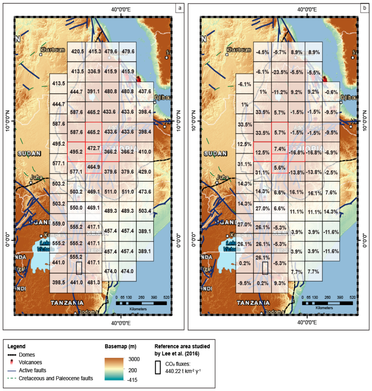
The statistical properties of the residuals and the extremely low mass density of the CO₂ molecules due to the Earth’s degassing allow us to assume a Poisson statistic for the distribution of carbon dioxide molecules in the atmosphere. The flow of CO₂ soil emissions is then estimated from the variance of the residuals, assuming an average CO₂ degassing velocity derived from calibrating satellite-based data against ground-based measurements in the Magadi-Natron basin. Figure 4 reports the CO₂ gradient of soil fluxes calculated for the different grid boxes (Figure 4a) and the percent differences from the measured values in the Magadi-Natron basin (Figure 4b). Comparison with ground measurements in very limited areas reported by Hunt in the Central and Northern Ethiopian Rift (MER) confirms a lower emission rate in this part of the rift system compared to the Southern Kenyan Rift, as captured by the satellite [43,44]. The estimated gradient of fluxes is provided solely for comparison with the ground-based measurements, confirming the presence of diffuse soil-degassing consistent with the satellite observations.

In Figure 4, the reduced area of some cells reflects the presence of small parts of the footprints with no measurements. In other areas, for regions with some missing or unreliable measurements, the NASA databank automatically interpolates data, using CO₂ profiles extracted from neighbouring areas. Both anomalies have been highlighted with red box borders. This overlap does not affect the scientific interpretation of the results. It has been reported only for completeness. Results show variations of up to 60% across different grid boxes, even in neighbouring areas, while regions with very similar degassing values indicate the highest fluxes along the main active tectonic structures.

This weak correlation confirms the interpretation of residuals as largely spatially independent of Earth’s diffuse surface degassing, while also reflecting the diffuse nature of time- and area-uncorrelated soil fluxes not limited to the borders of a single measurement area.

4.2. Continental Rifting and Deep CO₂ Lithospheric Degassing

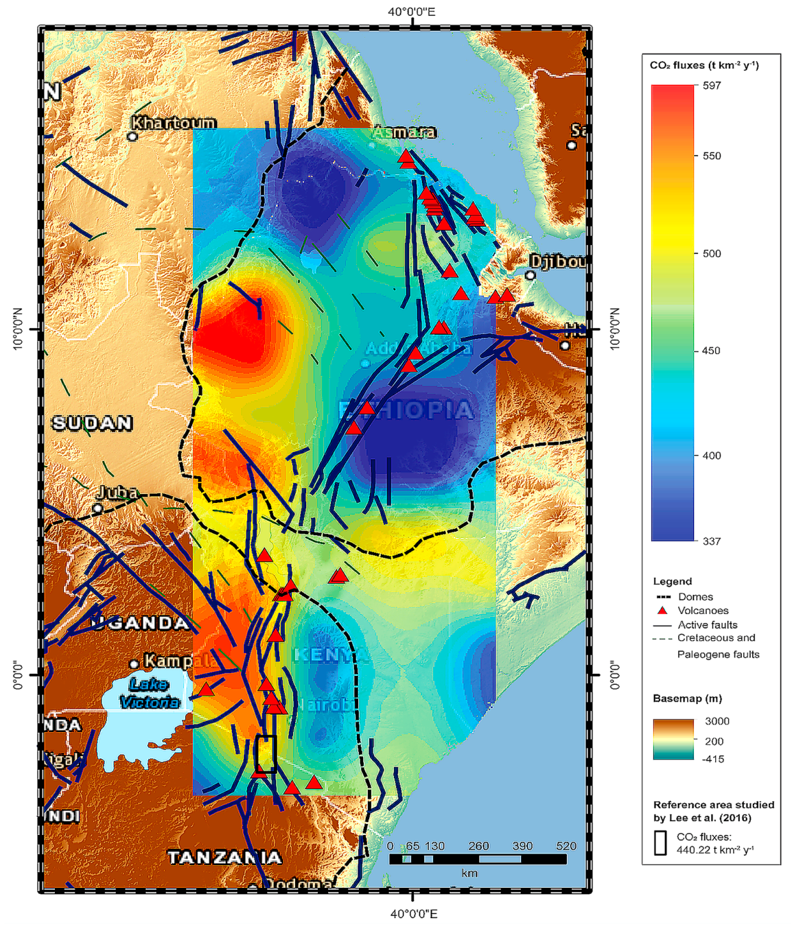
Figure 5 maps the diffuse CO₂ fluxes over the EAR, namely the Afar, the Ethiopian Rift, Turkana, and the Gregory Rift, and the adjacent Ethiopian and East African domes over an area of approximately 22 × 10⁵ km². Satellite observations reveal diffuse CO₂ emissions of variable intensity at the surface of the area under consideration, with the highest values aligned along major active tectonic structures.

Within the rift branches, measured CO₂ emissions are variable from 380 to 480 t km⁻² y⁻¹. Space measured CO₂ fluxes are comparable to ground-based measurements, and smaller in the northern part of the rift valley compared to the southern part of the rift valley [43,44]. Thus, the present results confirm that ground measurements over restricted regions cannot be reliably extrapolated to the entire EAR.

Notably, extended areas of CO₂ diffuse degassing have been identified over the Ethiopian plateau and the East African dome, with fluxes higher than those from the rift branches. Over the Ethiopian plateau (Figure 5), large amounts of CO₂ are released in areas of active fault systems, as far as 300 km from the western border of the rift. Similar high CO₂ fluxes are also measured in the East African dome region. The satellite image clearly shows that diffuse degassing is not restricted to the EAR but overlaps the distribution of the main active fault systems originating in the crust and mantle across the whole region affected by recent extensional tectonics. These findings are unexpected and cannot be explained by existing models that ascribe the origin of CO₂ to the deep degassing of mantle-derived basaltic magmas during their ascent to crustal levels [43,44]. Our results show that CO₂ degassing occurs over regions where magmatic activity ceased 5–19 My ago. We therefore argue that part of the CO₂ presently released to the atmosphere ascended from mantle depths through deep faults, even in the absence of active magmatism. The observed distribution can be interpreted within the geodynamic framework of continental rifting. Petrological evidence demonstrates that carbonate–silicate melt infiltration in the lithospheric mantle generated CO₂ in situ and that a melt-to-fluid transition occurred at mid-lithospheric depths [79,80]. Following exsolution, CO₂ fluids are expected to accumulate in the shallow lithosphere due to limited permeability in peridotitic matrices. Under these conditions, deep fault systems provide the most efficient pathways for CO₂ extraction. The close correspondence between satellite-derived fluxes and major tectonic structures supports a structurally controlled release of lithospherically stored carbon. This mechanism explains why diffuse degassing is detected over broad plateau regions and not solely along active volcanic segments. While the ultimate source of lithospheric carbon may relate to plume-derived carbonate-rich melts, remobilised subduction-related carbon, or a combination of both, the present observations indicate that the subcontinental lithosphere acts as a long-lived carbon reservoir capable of sustaining tectonically controlled degassing over geological timescales.

5. Conclusions

The statistical decomposition of long-term satellite-derived column CO₂ time series shows that diffuse surface degassing can be detected from space without ancillary ground measurements. The residual component isolated from the atmospheric column is stationary and spatially heterogeneous, and is statistically independent of seasonal biospheric cycles and long-term atmospheric trends.

Applied to the East African Rift region, this approach reveals a coherent spatial pattern of CO₂ fluxes aligned with major fault systems and extending into plateau areas where magmatism ceased millions of years ago. These results indicate that satellite column measurements, when properly decomposed, contain resolvable information about localised surface fluxes that would otherwise be masked by atmospheric mixing.

Independent petrological constraints support a lithospheric source for part of the observed degassing, involving carbonate–silicate melt infiltration and a subsequent melt-to-fluid transition at mid- to lower-lithospheric depths. The limited permeability of CO₂ fluids in peridotitic rocks implies structurally controlled extraction along deep fault systems, consistent with the spatial distribution of satellite-derived fluxes.

Overall, this study shows that statistical analysis of spaceborne CO₂ observations is a viable tool for identifying and mapping diffuse tectonic degassing across large regions. Although further calibration is needed to refine absolute flux magnitudes, the methodology offers new perspectives on quantifying natural carbon emissions at regional to continental scales and on integrating satellite observations with solid-Earth processes.

References

1. WMO GAW Programme. Available online: https://community.wmo.int/site/knowledge-hub/programmes-and-initiatives/global-atmosphere-watch-gaw-programme?utm_source=chatgpt.com (accessed on 10 June 2026).
2. WDCGG Data Portal. Available online: https://community.wmo.int/site/knowledge-hub/programmes-and-initiatives/global-atmosphere-watch-gaw-programme/world-data-centre-greenhouse-gases?utm_source=chatgpt.com (accessed on 10 June 2026).
3. Observation Package (ObsPack) Data Products. Available online: https://gml.noaa.gov/ccgg/obspack/data.php (accessed on 10 June 2026).
4. NOAA GML CO2 Data; CO2 Trends (Mauna Loa etc.). Available online: https://gml.noaa.gov/ccgg/trends/?utm_source=chatgpt.com (accessed on 10 June 2026).
5. Total Carbon Column Observing Network (TCCON) Wiki. Available online: https://tccon-wiki.caltech.edu (accessed on 10 June 2026).
6. Standardised Greenhouse Gas Measurements Throughout Europe. Available online: https://www.icos-cp.eu (accessed on 10 June 2026).
7. COllaborative Carbon Column Observing Network (COCCON). Available online: https://www.coccon.kit.edu/?utm_source=chatgpt.com (accessed on 10 June 2026).
8. FLUXNET. Available online: https://fluxnet.org (accessed on 10 June 2026).
9. Available online: https://ocov2.jpl.nasa.gov (accessed on 10 June 2026).
10. Available online: https://ocov3.jpl.nasa.gov (accessed on 10 June 2026).
11. Greenhouse Gases Observing Satellite GOSAT “IBUKI”. Available online: https://www.gosat.nies.go.jp/en/ (accessed on 10 June 2026).
12. Available online: https://science.nasa.gov/mission/oco/ (accessed on 10 June 2026).
13. National Satellite Meteorological Center (NSMC), China Meteorological Administration. TanSat (Carbon Dioxide Observation Satellite). Available online: https://www.nsmc.org.cn/nsmc/en/satellite/TanSat.htm (accessed on 10 June 2026).
14. SCIAMACHY. Available online: https://www.sciamachy.org/ (accessed on 10 June 2026).
15. AIRS. Available online: https://airs.jpl.nasa.gov (accessed on 10 June 2026).
16. IASI. Available online: https://cnes.fr/projets/iasi (accessed on 10 June 2026).
17. European Organisation for the Exploitation of Meteorological Satellites (EUMETSAT). CO2M (Copernicus CO2 Monitoring Mission). Available online: https://www.eumetsat.int/co2m (accessed on 10 June 2026).
18. MicroCarb. Available online: https://microcarb.cnes.fr/en (accessed on 10 June 2026).
19. Yang, D.; Zhang, H.; Liu, Y.; Chen, B.; Cai, Z.; Lü, D. Monitoring carbon dioxide from space: Retrieval algorithm and flux inversion based on GOSAT data and using CarbonTracker-China. Adv. Atmos. Sci. 2017, 34, 965–976. [Google Scholar] [CrossRef] [Scilit]
20. Eldering, A.; Wennberg, P.O.; Crisp, D.; Schimel, D.S.; Gunson, M.R.; Chatterjee, A.; Liu, J.; Schwandner, F.M.; Sun, Y.; O’dEll, C.W.; et al. The Orbiting Carbon Observatory-2 early science investigations of regional carbon dioxide. Science 2017, 358, eaam5745. [Google Scholar] [CrossRef] [Scilit] [PubMed]
21. Rodgers, C.D. Inverse Methods for Atmospheric Sounding: Theory and Practice; World Scientific Publishing: Singapore; River Edge, NJ, USA, 2000. [Google Scholar] [CrossRef]
22. Chevallier, F.; Engelen, R.J.; Peylin, P. Inferring CO2 sources and sinks from satellite observations: Method and application to TOVS data. J. Geophys. Res. Atmos. 2005, 110, D24309. [Google Scholar] [CrossRef] [Scilit]
23. Peylin, P.; Law, R.M.; Gurney, K.R.; Chevallier, F.; Jacobson, A.R.; Maki, T.; Niwa, Y.; Patra, P.K.; Peters, W.; Rayner, P.J.; et al. Global atmospheric carbon budget: Results from an ensemble of atmospheric CO2 inversions. Biogeosciences 2013, 10, 6699–6720. [Google Scholar] [CrossRef] [Scilit]
24. Crowell, S.; Baker, D.F.; Schuh, A.E.; Basu, S.; Jacobson, A.R.; Chevallier, F.; Liu, J.; Deng, F.; Feng, L.; Chatterjee, A.; et al. The 2015–2016 carbon cycle as seen from OCO-2 and the global in situ network. Atmos. Chem. Phys. 2019, 19, 9797–9831. [Google Scholar] [CrossRef] [Scilit]
25. Nassar, R.; Hill, T.G.; McLinden, C.A.; Wunch, D.; Chen, J.; Xu, X. Quantifying CO2 emissions from individual power plants from space. Geophys. Res. Lett. 2017, 44, 10045–10053. [Google Scholar] [CrossRef] [Scilit]
26. Crisp, D.; Fisher, B.M.; O’Dell, C.; Frankenberg, C.; Basilio, R.; Bösch, H.; Brown, L.R.; Castano, R.; Connor, B.; Deutscher, N.M. The ACOS CO2 retrieval algorithm—Part II: Global XCO2 data characterization. Atmos. Meas. Tech. 2012, 5, 687–707. [Google Scholar] [CrossRef] [Scilit]
27. Connor, B.J.; Boesch, H.; Toon, G.; Sen, B.; Miller, C.; Crisp, D. Orbiting Carbon Observatory: Inverse method and prospective error analysis. J. Geophys. Res. Atmos. 2008, 113, D05305. [Google Scholar] [CrossRef] [Scilit]
28. Kulawik, S.S.; O’Dell, C.; Nelson, R.R.; Taylor, T.E. Validation of OCO-2 error analysis using simulated retrievals. Atmos. Meas. Tech. 2019, 12, 5317–5334. [Google Scholar] [CrossRef] [Scilit]
29. Chédin, A.; Serrar, S.; Scott, N.A.; Crevoisier, C.; Armante, R. First global measurement of midtropospheric CO2 from NOAA polar satellites: Tropical zone. J. Geophys. Res. Atmos. 2003, 108, 4581. [Google Scholar] [CrossRef] [Scilit]
30. Chahine, M.T.; Pagano, T.S.; Aumann, H.H.; Atlas, R.; Barnet, C.; Blaisdell, J.; Chen, L.; Divakarla, M.; Fetzer, E.J.; Goldberg, M.; et al. AIRS: Improving weather forecasting and providing new data on greenhouse gases. Bull. Am. Meteorol. Soc. 2006, 87, 911–926. [Google Scholar] [CrossRef] [Scilit]
31. Crevoisier, C.; Heilliette, S.; Chédin, A.; Serrar, S.; Armante, R.; Scott, N.A. Midtropospheric CO2 concentration retrieval from AIRS observations in the tropics. Geophys. Res. Lett. 2004, 31, L17106. [Google Scholar] [CrossRef] [Scilit]
32. Byrne, B.; Jones, D.B.A.; Strong, K.; Zeng, Z.-C.; Deng, F.; Liu, J. Sensitivity of CO2 surface flux constraints to observational coverage. J. Geophys. Res. Atmos. 2017, 122, 6672–6694. [Google Scholar] [CrossRef] [Scilit]
33. Friedlingstein, P.; O’SUllivan, M.; Jones, M.W.; Andrew, R.M.; Bakker, D.C.E.; Hauck, J.; Landschützer, P.; Le Quéré, C.; Luijkx, I.T.; Peters, G.P.; et al. Global Carbon Budget. Earth Syst. Sci. Data 2023, 15, 5301–5369. [Google Scholar] [CrossRef] [Scilit]
34. Wunch, D.; Toon, G.C.; Blavier, J.-F.L.; Washenfelder, R.A.; Notholt, J.; Connor, B.J.; Griffith, D.W.T.; Sherlock, V.; Wennberg, P.O. The Total Carbon Column Observing Network. Philos. Trans. R. Soc. A Math. Phys. Eng. Sci. 2011, 369, 2087–2112. [Google Scholar] [CrossRef] [Scilit] [PubMed]
35. Duren, R.M.; Miller, C.E. Measuring the carbon emissions of megacities. Nat. Clim. Change 2012, 2, 560–562. [Google Scholar] [CrossRef] [Scilit]
36. Deng, F.; Jones, D.B.A.; Henze, D.K.; Bousserez, N.; Bowman, K.W.; Fisher, J.B.; Nassar, R.; O’Dell, C.; Wunch, D.; Wennberg, P.O.; et al. Inferring regional sources and sinks of atmospheric CO2 from GOSAT XCO2 data. Atmos. Chem. Phys. 2014, 14, 3703–3727. [Google Scholar] [CrossRef] [Scilit]
37. Schwandner, F.M.; Gunson, M.R.; Miller, C.E.; Carn, S.A.; Eldering, A.; Krings, T.; Verhulst, K.R.; Schimel, D.S.; Nguyen, H.M.; Crisp, D.; et al. Spaceborne detection of localized CO2 sources. Science 2017, 358, eaam5782. [Google Scholar] [CrossRef] [Scilit] [PubMed]
38. Werner, C.; Fischer, T.P.; Aiuppa, A.; Edmonds, M.; Cardellini, C.; Carn, S.; Chiodini, G.; Cottrell, E.; Burton, M.; Shinohara, H.; et al. Carbon Dioxide Emissions from Subaerial Volcanic Regions. In Deep Carbon: Past to Present; Orcutt, B.N., Daniel, I., Dasgupta, R., Eds.; Cambridge University Press: Cambridge, UK, 2019; Chapter 8; pp. 188–236. [Google Scholar] [CrossRef] [Scilit]
39. Romaniello, V.; Ganci, G. Exploitation of OCO-3 satellite data to analyse carbon dioxide emissions from the Mt. Etna volcano. Remote Sens. 2025, 17, 1918. [Google Scholar] [CrossRef] [Scilit]
40. Malusà, M.G.; Frezzotti, M.L.; Ferrando, S.; Brandmayr, E.; Romanelli, F.; Panza, G.F. Active carbon sequestration in the Alpine mantle wedge and implications for long-term climate trends. Sci. Rep. 2018, 8, 4740. [Google Scholar] [CrossRef] [Scilit] [PubMed]
41. Moretti, R.; Métrich, N.; Arienzo, I.; Di Renzo, V.; Aiuppa, A.; Allard, P. Degassing vs. eruptive styles at Mt. Etna volcano (Sicily, Italy). Part I: Volatile stocking, gas fluxing, and the shift from low-energy to highly explosive basaltic eruptions. Chem. Geol. 2018, 482, 1–17. [Google Scholar] [CrossRef] [Scilit]
42. Brune, S.; Williams, S.E.; Müller, R.D. Potential links between continental rifting, CO2 degassing and climate change through time. Nat. Geosci. 2017, 10, 941–946. [Google Scholar] [CrossRef] [Scilit]
43. Hunt, J.A.; Zafu, A.; Mather, T.A.; Pyle, D.M.; Barry, P.H. Spatially variable CO2 degassing in the Main Ethiopian Rift: Implications for magma storage, volatile transport and rift-related emissions. Geochem. Geophys. Geosyst. 2017, 18, 3714–3737. [Google Scholar] [CrossRef] [Scilit]
44. Lee, H.; Muirhead, J.D.; Fischer, T.P.; Ebinger, C.J.; Kattenhorn, S.A.; Sharp, Z.D.; Kianji, G. Massive and prolonged deep carbon emissions associated with continental rifting. Nat. Geosci. 2016, 9, 145–149. [Google Scholar] [CrossRef] [Scilit]
45. Baker, J.; Chazot, G.; Menzies, M.; Thirlwall, M. Metasomatism of the shallow mantle beneath Yemen by the Afar plume: Implications for mantle plumes, flood volcanism, and intraplate volcanism. Geology 1998, 26, 431–434. [Google Scholar] [CrossRef] [Scilit]
46. Rooney, T.O.; Furman, T.; Yirgu, G.; Ayalew, D. Structure of the Ethiopian lithosphere: Xenolith evidence in the Main Ethiopian Rift. Geochim. Cosmochim. Acta 2005, 69, 3889–3910. [Google Scholar] [CrossRef] [Scilit]
47. Ferrando, S.; Frezzotti, M.L.; Neumann, E.-R.; De Astis, G.; Peccerillo, A.; Dereje, A.; Gezahegn, Y.; Teklewold, A. Composition and thermal structure of the lithosphere beneath the Ethiopian plateau: Evidence from mantle xenoliths in basanites, Injibara, Lake Tana Province. Mineral. Petrol. 2008, 93, 47–78. [Google Scholar] [CrossRef] [Scilit]
48. Fischer, T.P.; Burnard, P.; Marty, B.; Hilton, D.R.; Füri, E.; Palhol, F.; Sharp, Z.D.; Mangasini, F. Upper-mantle volatile chemistry at Oldoinyo Lengai volcano and the origin of carbonatites. Nature 2009, 459, 77–80. [Google Scholar] [CrossRef] [Scilit] [PubMed]
49. Muirhead, J.D.; Kattenhorn, S.; Lee, H.; Mana, S.; Turrin, B.; Fischer, T.; Kianji, G.; Dindi, E.; Stamps, D. Evolution of upper crustal faulting assisted by magmatic volatile release during early-stage continental rift development in the East African Rift. Geosphere 2016, 12, 1670–1700. [Google Scholar] [CrossRef] [Scilit]
50. Bedini, R.M.; Bodinier, J.L.; Dautria, J.M.; Morten, L. Evolution of LILE-enriched small melt fractions in the lithospheric mantle: A case study from the East African Rift. Earth Planet. Sci. Lett. 1997, 153, 67–83. [Google Scholar] [CrossRef] [Scilit]
51. Hammouda, T.; Laporte, D. Ultrafast mantle impregnation by carbonatite melts. Geology 2000, 28, 283–286. [Google Scholar] [CrossRef] [Scilit]
52. Casagli, A.; Frezzotti, M.L.; Peccerillo, A.; Tiepolo, M.; De Astis, G. Garnet-spinel peridotite xenoliths from Mega (Ethiopia): Evidence for rejuvenation and dynamic thinning of the lithosphere beneath the southern Main Ethiopian Rift. Chem. Geol. 2017, 455, 231–248. [Google Scholar] [CrossRef] [Scilit]
53. Maffeis, A.; Frezzotti, M.L.; Esposito, R.; Malusà, M.G.; Aiuppa, A.; Rizzo, A.L.; Ferrando, S. Carbon enrichment processes in the oceanic upper mantle preserved in peridotites from Sal Island (Cape Verde). Geosci. Front. 2026, 17, 102179. [Google Scholar] [CrossRef] [Scilit]
54. R Core Team. R: A Language and Environment for Statistical Computing. R Foundation for Statistical Computing. Available online: https://www.R-project.org/ (accessed on 10 June 2026).
55. Dickey, D.A.; Fuller, W.A. Distribution of the estimators for autoregressive time series with a unit root. J. Am. Stat. Assoc. 1979, 74, 427–431. [Google Scholar] [CrossRef] [Scilit]
56. Kwiatkowski, D.; Phillips, P.C.B.; Schmidt, P.; Shin, Y. Testing the null hypothesis of stationarity against the alternative of a unit root. J. Econom. 1992, 54, 159–178. [Google Scholar] [CrossRef] [Scilit]
57. Zhang, L.; Jiang, H.; Zhang, X. Comparison analysis of the global carbon dioxide concentration column derived from SCIAMACHY, AIRS, and GOSAT with surface station measurements. Int. J. Remote Sens. 2015, 36, 1406–1423. [Google Scholar] [CrossRef] [Scilit]
58. Chahine, M.T.; Chen, L.; Dimotakis, P.; Jiang, X.; Li, Q.; Olsen, E.T.; Pagano, T.; Randerson, J.T.; Yung, Y.L. Satellite remote sounding of mid-tropospheric CO2. Geophys. Res. Lett. 2008, 35, L17807. [Google Scholar] [CrossRef] [Scilit]
59. Acker, J.G.; Leptoukh, G.G. Online analysis enhances use of NASA Earth science data. Eos Trans. Am. Geophys. Union 2007, 88, 14–17. [Google Scholar] [CrossRef] [Scilit]
60. Wojdyr, M. Fityk: A general-purpose peak fitting program. J. Appl. Crystallogr. 2010, 43, 1126–1128. [Google Scholar] [CrossRef] [Scilit]
61. Frezzotti, M.-L.; Tecce, F.; Casagli, A. Raman spectroscopy for fluid inclusion analysis. J. Geochem. Explor. 2012, 112, 1–20. [Google Scholar] [CrossRef] [Scilit]
62. Trapletti, A.; Hornik, K. Tseries: Time Series Analysis and Computational Finance. R package version 0.10-45. 2018. Available online: https://CRAN.R-project.org/package=tseries (accessed on 10 June 2026).
63. Hamilton, J.D. Time Series Analysis; Princeton University Press: Princeton, NJ, USA, 1994. [Google Scholar]
64. Keeling, C.D. The concentration and isotopic abundances of carbon dioxide in the atmosphere. Tellus 1960, 12, 200–203. [Google Scholar] [CrossRef] [Scilit]
65. Buchwitz, M.; Reuter, M.; Schneising, O.; Noël, S.; Gier, B.; Bovensmann, H.; Burrows, J.P.; Boesch, H.; Anand, J.; Parker, R.J.; et al. Computation and analysis of atmospheric carbon dioxide annual mean growth rates from satellite observations during 2003–2016. Atmos. Chem. Phys. 2018, 18, 17355–17370. [Google Scholar] [CrossRef] [Scilit]
66. Patra, P.K.; Crisp, D.; Kaiser, J.W.; Wunch, D.; Saeki, T.; Ichii, K.; Sekiya, T.; Wennberg, P.O.; Feist, D.G.; Pollard, D.F.; et al. The Orbiting Carbon Observatory (OCO-2) tracks 2–3 petagram increase in carbon release to the atmosphere during the 2014–2016 El Niño. Sci. Rep. 2017, 7, 13567. [Google Scholar] [CrossRef] [Scilit] [PubMed]
67. Eldering, A.; O’Dell, C.W.; Wennberg, P.O.; Crisp, D.; Gunson, M.R.; Viatte, C.; Avis, C.; Braverman, A.; Castano, R.; Chang, A.; et al. The Orbiting Carbon Observatory-2: First 18 months of science data products. Atmos. Meas. Tech. 2017, 10, 549–563. [Google Scholar] [CrossRef] [Scilit]
68. Liu, M.; Wu, J.; Zhu, X.; He, H.; Jia, W.; Xiang, W. Evolution and variation of atmospheric carbon dioxide concentration over terrestrial ecosystems as derived from eddy covariance measurements. Atmos. Environ. 2015, 114, 75–82. [Google Scholar] [CrossRef] [Scilit]
69. Jiang, X.; Crisp, D.; Olsen, E.T.; Kulawik, S.S.; Miller, C.E.; Pagano, T.S.; Liang, M.; Yung, Y.L.; Chahine, M.T. CO2 annual and semiannual cycles from multiple satellite retrievals and models. Earth Space Sci. 2016, 3, 78–87. [Google Scholar] [CrossRef] [Scilit]
70. Peng, S.; Ciais, P.; Chevallier, F.; Peylin, P.; Cadule, P.; Sitch, S.; Piao, S.; Ahlström, A.; Huntingford, C.; Levy, P.; et al. Benchmarking the seasonal cycle of CO2 fluxes simulated by terrestrial ecosystem models. Glob. Biogeochem. Cycles 2015, 29, 46–64. [Google Scholar] [CrossRef] [Scilit]
71. Schneising, O.; Reuter, M.; Buchwitz, M.; Heymann, J.; Bovensmann, H.; Burrows, J.P. Terrestrial carbon sink observed from space: Variation of growth rates and seasonal cycle amplitudes in response to interannual surface temperature variability. Atmos. Chem. Phys. 2014, 14, 133–141. [Google Scholar] [CrossRef] [Scilit]
72. Landau, L.; Lifchitz, E. Physique Statistique; Editions Mir: Moscou, Russia, 1967. [Google Scholar]
73. Bird, G.A. Molecular Gas Dynamics and the Direct Simulation of Gas Flows; Oxford University Press: Oxford, UK, 1994. [Google Scholar]
74. Chabala, L.M.; Mulolwa, A.; Lungu, O. Application of Ordinary Kriging in Mapping Soil Organic Carbon in Zambia. Pedosphere 2017, 27, 338–343. [Google Scholar] [CrossRef] [Scilit]
75. Johnston, K.; Ver Hoef, J.M.; Krivoruchko, K.; Lucas, N. Using ArcGIS Geostatistical Analyst; ESRI: Redlands, CA, USA, 2001. [Google Scholar]
76. Cressie, N. Spatial prediction and ordinary kriging. Math. Geol. 1988, 20, 405–421. [Google Scholar] [CrossRef] [Scilit]
77. Wackernagel, H. Multivariate Geostatistics: An Introduction with Applications, 3rd ed.; Springer: Berlin, Germany, 2013. [Google Scholar] [CrossRef] [Scilit]
78. van Beers, W.C.M.; Kleijnen, J.P.C. Kriging for interpolation in random simulation. J. Oper. Res. Soc. 2003, 54, 255–262. [Google Scholar] [CrossRef] [Scilit]
79. Tamburello, G.; Pondrelli, S.; Chiodini, G.; Rouwet, D. Global-scale control of extensional tectonics on CO2 Earth degassing. Nat. Commun. 2018, 9, 4608. [Google Scholar] [CrossRef] [Scilit] [PubMed]
80. Stagno, V.; Ojwang, D.O.; McCammon, C.A.; Frost, D.J. The oxidation state of the mantle and the extraction of carbon from Earth’s interior. Nature 2013, 493, 84–88. [Google Scholar] [CrossRef] [Scilit] [PubMed]
Figure 1. (A) Total signal. (B) Autocorrelation functions for the residual x r e s i d u a l , i . (C) Autocorrelation functions for the squared residual x r e s i d u a l , i 2 . (D) Autocorrelation functions for the biquadratic of residuals x r e s i d u a l , i 4 for grid box [Northeastern Plateau; (36.66–38.2°)E; (13.33–15°)N], blue line in Figure 2.
Remotesensing 18 02586 g001
Figure 2. Decomposition of the total signal as measured by the satellite as a function of time for three different grid boxes: grid box 1 with red line (South Eastern Plateau 35–36.66°E; 9–10.66°N), grid box 2 with blue line (Nord Eastern Plateau; 36.66–38.2°E; 13.33–15°N), and grid box 3 with violet line (South Western Plateau; 39.8–41.4°E; 6.68–8.34°N) and corresponding to the column-averaged atmospheric CO2 content: panel (A), total signal; panel (B), trend of the global-averaged increase in the total CO2 concentration mixed by the atmospheric circulation; panel (C), seasonal time- synchronous annual and semi-annual oscillations corresponding to the vegetation cycle; panel (D), residues of the signals in the grid box 1, 2, and 3.
Remotesensing 18 02586 g002
Figure 3. Scatter-gram of residuals calculated for two adjacent grid boxes. The diagram reports the values of the residuals calculated at the same time for two different neighbouring grid boxes.
Remotesensing 18 02586 g003
Figure 4. Maps of measured satellite footprint areas and residuals. (a) Estimated diffuse CO2 fluxes measured by the AIRS/AQUA NASA satellite over seventy footprint areas; (b) percent difference in CO2 fluxes calculated with respect to the Magadi-Natron reference area [44]. Cells with red borders indicate regions where the NASA databank automatically interpolates CO2 some profiles using data from neighbouring areas. This does not affect the scientific interpretation of the results, and it has been reported only for completeness.
Remotesensing 18 02586 g004
Figure 5. Variation map of the diffuse CO2 estimated fluxes in East Africa (reference area [44]). The variation in CO2 fluxes (blue to red shaded scale) is obtained by the interpolation of measured CO2 emissions over the Eastern branch of the EARS) with the Ordinary Kriging geostatistical tool in ArcGIS 10.6 [74,75].
Remotesensing 18 02586 g005