A Study on Radar–Gauge Rainfall Data Merging and Its Impact on Flood Simulation

Highlights

What are the main findings?

• All three radar–gauge fusion methods (GDA, CM, RF) substantially corrected the systematic underestimation in radar QPE. Under leave-one-gauge-out cross-validation, GDA and CM exhibited similar and robust point-scale accuracy (overall CC ≈ 0.81), whereas RF showed substantially lower generalization (CC ≈ 0.48).
• In HEC-HMS flood simulations, GDA-fused rainfall delivered the most robust overall performance across diverse flood types, while all three fused products consistently outperformed single-source rainfall inputs.

What are the implications of the main findings?

• Radar–gauge data fusion provides a reliable pathway to enhance rainfall input quality and improve operational flood forecasting in semi-arid watersheds.
• Independent cross-validation reveals a notable contrast: while CM marginally achieved the highest statistical accuracy (overall CC ≈ 0.81 for point scale, CC ≈ 0.96 for basin scale), GDA delivered the most robust flood simulations. This finding demonstrates that optimal statistical fidelity does not automatically translate into optimal hydrological performance, underscoring the importance of application-oriented validation when evaluating rainfall fusion methods.

Abstract

Accurate rainfall input is critical for reliable flood simulation, particularly in semi-arid watersheds with pronounced spatiotemporal precipitation heterogeneity. This study developed a radar–gauge rainfall fusion framework to improve HEC-HMS (Hydrologic Engineering Center–Hydrologic Modeling System) model performance in the Liulin experimental watershed, Xingtai City, Hebei Province. Radar quantitative precipitation estimation (QPE) was generated via a dynamically optimized Z-I relationship, then fused with gauge observations using three methods—Geographical Differential Analysis (GDA), Conditional Merging (CM), and Random Forest (RF). The fused products drove a calibrated HEC-HMS model, evaluated over five representative flood events. All three methods corrected radar QPE underestimation. Under independent cross-validation, GDA and CM achieved comparable point-scale accuracy (CC ≈ 0.81, RMSE ≈ 5.7 mm), while RF showed lower generalization (CC ≈ 0.48, RMSE ≈ 8.7 mm) due to overfitting. In flood simulations, GDA performed most robustly, followed by RF and CM, all surpassing single-source inputs. Notably, CM’s higher statistical accuracy did not translate into better flood performance, indicating that optimal statistical fidelity does not guarantee optimal hydrological results. Peak discharge deviations persisted for short-duration intense storms and long-duration uneven rainfall events. This study confirms that radar–gauge fusion enhances rainfall input quality and provides a reliable approach for improving flood forecasting.

1. Introduction

The escalating frequency and intensity of extreme precipitation events globally [1,2,3] heightens the demand for accurate flood forecasting, a critical tool for mitigating socio-economic losses [4,5,6]. The predictive skill of hydrological models is fundamentally contingent on rainfall input quality [7,8], yet capturing the inherent spatiotemporal heterogeneity of precipitation remains a persistent observational challenge [9].

Point measurements from rain gauge networks serve as the benchmark for accuracy but offer limited spatial representativeness, introducing substantial uncertainty into watershed modeling [10]. Satellite-based precipitation products provide global coverage without ground infrastructure, yet their relatively coarse spatiotemporal resolution limits their capacity to resolve short-duration, convective storms typical of flash flood events [11]. Weather radar technology, by contrast, has advanced substantially over the past two decades. Radar-derived QPE combines high spatiotemporal resolution with extensive areal coverage, enabling real-time monitoring of regional precipitation distribution [12,13], and has consequently been widely adopted in hydrological modeling and flood forecasting research [14,15,16].

The core of radar QPE lies in the empirical relationship between the radar reflectivity factor (Z) and rainfall intensity (I). Since the foundational Marshall–Palmer relationship (Z = 200I^1.6) was proposed by Marshall et al. [17], it has been recognized that a single, static Z-I relationship cannot capture the microphysical diversity of precipitation regimes. This drove a progression from regime-specific formulations—such as the convective rainfall relationship (Z = 300I^1.4) proposed by Joss et al. [18]—to dynamically optimized approaches that calibrate Z-I parameters in near real-time using the most recent gauge–radar comparisons. Such dynamic methods inherently account for evolving weather systems and local topographic influences [19], outperforming fixed, single-parameter relationships. The subsequent introduction of dual-polarization radar technology further enhanced QPE capability [20,21], while machine learning methods have more recently opened new development pathways in this field [22,23].

Radar QPE, however, is susceptible to multiple error sources [24,25], including hardware system errors, beam-geometry-induced errors such as beam broadening and signal attenuation with increasing range [25,26,27], non-meteorological echoes from ground clutter, electromagnetic interference, and biological targets [7,28,29,30], and signal degradation due to terrain occlusion and anomalous propagation [31,32,33,34]. To mitigate these errors, specialized software for processing three-dimensional radar reflectivity data has been developed to remove non-meteorological echoes and correct for beam blockage and attenuation [35,36]. Beyond internal correction, incorporating ground-based rain gauge observations provides an effective means to reduce systematic biases and improve QPE accuracy, thereby driving the development of multi-source precipitation data fusion techniques [37].

Radar–gauge merging methods can be broadly categorized into three types based on their fusion strategy: radar bias correction methods, geostatistical methods, and statistical integration methods [38,39,40,41,42,43,44]. Bias correction methods use gauge observations as a benchmark to adjust systematic radar biases. The Mean Field Bias (MFB) approach assumes spatially uniform radar error and applies a single correction factor derived from the average gauge-to-radar ratio [45,46]. To address spatial error heterogeneity, researchers developed distance-dependent and local bias correction methods—the latter obtain local correction factors by interpolating radar–gauge differences at gauge locations, employing techniques such as negative exponential weighting [47] or multiquadric surface fitting [48]—as radar estimation bias has been shown to increase with distance [49]. Geostatistical methods, rather than treating radar as a background field, utilize its spatial structure to assist gauge data interpolation. Kriging with External Drift (KED) employs radar QPE as an auxiliary variable to constrain interpolation weights [50], while Conditional Merging (CM) uses the difference between the original radar field and a Kriging-interpolated radar field to correct the gauge-based Kriging rainfall field, thereby reducing interpolation error [51]. Integration methods, including CoKriging (CoK) and Bayesian Data Merging (BAY), aim to minimize overall estimation uncertainty by incorporating both data sources into a unified framework—CoK through a joint Kriging system that minimizes estimation error variance [52,53], and BAY through optimal fusion within a Bayesian framework that separately quantifies the uncertainty of each data source [54].

A critical gap remains in the systematic, multi-method evaluation of these fusion products within a fully calibrated hydrological modeling chain. The ultimate utility of a fused rainfall product is not defined solely by its pixel-level statistical agreement with gauge observations but by its capacity to improve physically meaningful hydrological outputs. This study addresses this gap through a rigorous intercomparison in the Liulin experimental watershed, a well-characterized, flood-prone semi-arid catchment. The specific objectives are to: (1) generate and evaluate radar QPE using a dynamically optimized Z-I relationship; (2) develop and compare three conceptually distinct fusion methods—GDA, CM, and RF—for radar–gauge rainfall data integration; and (3) comprehensively assess their performance in driving a calibrated HEC-HMS (Hydrologic Engineering Center–Hydrologic Modeling System) hydrological model across diverse flood event types, and to evaluate the relationship between independent statistical accuracy and hydrological utility, thereby quantifying the added value of data fusion for operational flood forecasting.

2. Materials and Methods

2.1. Study Area

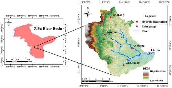
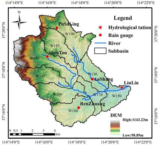
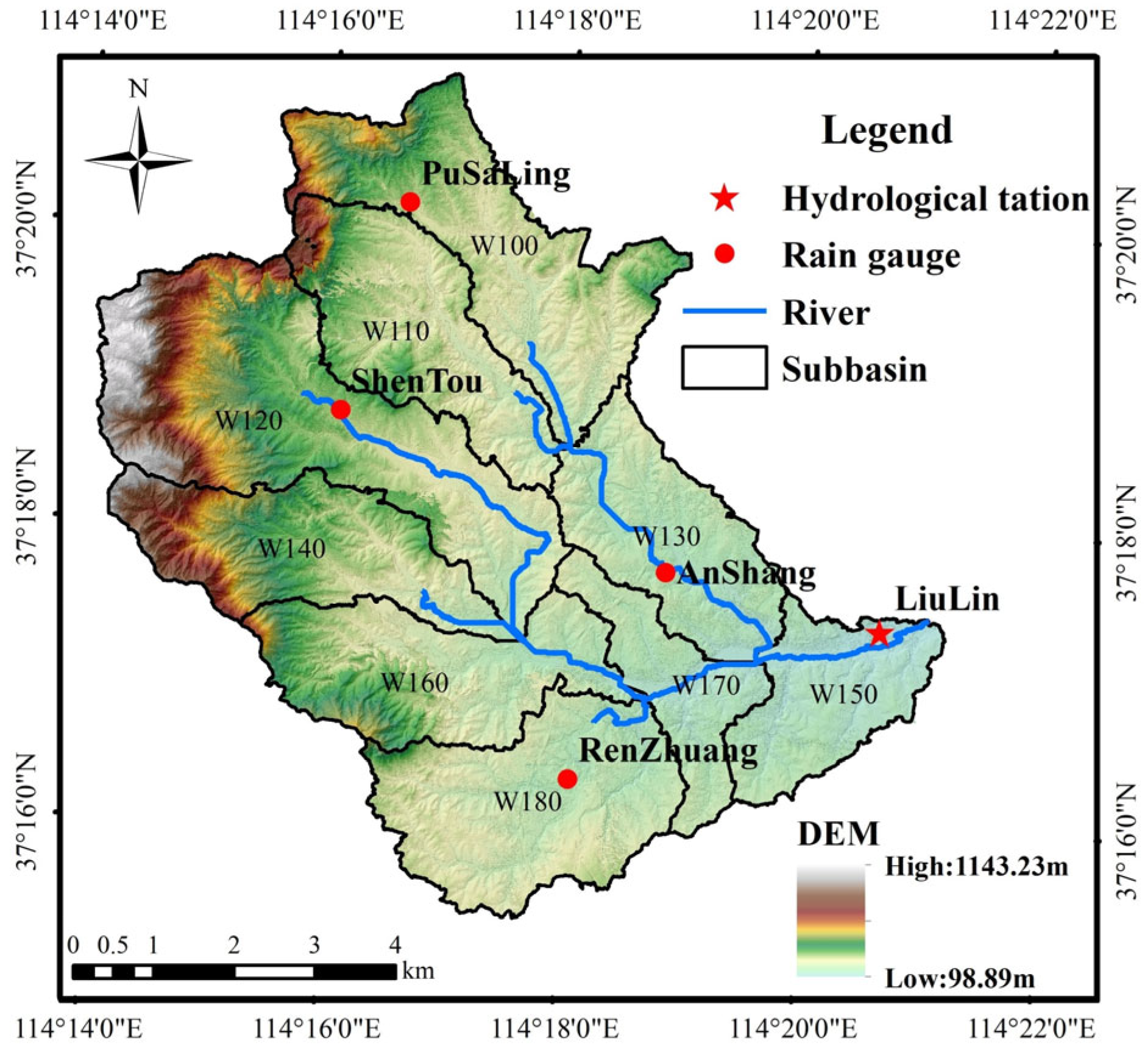
The Liulin experimental watershed is located in Neiqiu County, Xingtai City, Hebei Province, and forms part of the Xiaoma River system within the Ziya River basin of the Haihe River watershed. The river originates from Taiziyan Mountain on the eastern flank of the Taihang Mountains. The watershed exhibits a pronounced west-to-east elevation gradient, with a drainage area of 57.4 km², a main channel length of 13.2 km, an average slope of 30.9‰, and a watershed width of 4.35 km. Figure 1 shows the location and monitoring infrastructure of the study area.

Figure 1. Location and Station Distribution of Liulin Basin.

The Xiaoma River is a seasonal stream, with floods concentrated from June to September and peaking most frequently in late July to early August. The watershed’s multi-year average precipitation is 594.5 mm, with a multi-year average runoff depth of 80.7 mm. The multi-year average maximum 24 h and 3-day rainfall totals are 92.5 mm and 135 mm, respectively. Multi-year average water surface evaporation reaches 1045.5 mm. The recorded maximum peak discharge of 570 m³/s occurred in 1996.

The watershed outlet (114°21′E, 37°17′N) is instrumented with the Liulin Hydrological Station, which provides continuous water level and discharge observations. Five rain gauge stations—Pusaling, Shentou, Anshang, Liulin, and Renzhuang—are distributed within the watershed for precipitation monitoring. The spatial configuration of these stations is shown in Figure 1.

2.2. Data Acquisition and Preprocessing

The dataset assembled for this study integrates topographic, hydrologic, and meteorological observations. A high-resolution (1 m) Digital Elevation Model (DEM) was generated from Unmanned Aerial Vehicle (UAV) oblique photogrammetry to underpin hydrological model construction.

Hourly rainfall records from the five internal rain gauge stations and concurrent hourly discharge data from the Liulin Hydrological Station were compiled for the flood seasons from 1995 to 2023. From this long-term archive, 22 typical flood events spanning various hydrograph shapes and magnitudes were selected for model calibration and validation.

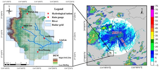
Radar data were obtained from the Shijiazhuang S-band Doppler weather radar (114°42′50″E, 38°21′00″N), which is part of the China Next Generation Weather Radar (CINRAD) network. The radar was manufactured by Huayun Metstar Radar (Beijing) Co., Ltd., Beijing, China. The radar operates in precipitation mode with Volume Coverage Pattern 21 (VCP21), completing a volume scan of nine elevation angles (0.5°, 1.5°, 2.4°, 3.4°, 4.3°, 6.0°, 9.9°, 14.6°, 19.5°) every 6 min. The effective detection radius is 230 km, with a radial resolution of 1 km and an azimuthal resolution of approximately 1°. The Liulin watershed (57.4 km²) lies entirely within 120 km of the radar and is covered by approximately 70 radar grid cells (Figure 2). The radar data are stored in a standard binary base-data format, which requires dedicated decoding and coordinate transformation before quantitative analysis. The raw radar base data were decoded and processed using the open-source PyCWR package (https://github.com/YvZheng/pycwr, accessed on 25 July 2026, version 1.0.8). A Constant Altitude Plan Position Indicator (CAPPI) product at a constant altitude of 3 km above mean sea level was then generated by interpolating the decoded reflectivity from the multiple elevation scans onto a Cartesian grid with 1 km horizontal spacing using an inverse distance weighting (IDW) method. This altitude was chosen because it lies above the ridgeline of the surrounding Taihang Mountains for most of the watershed, thereby mitigating low-level beam blockage effects. The use of a 3 km CAPPI, rather than the lowest elevation scan, helps mitigate the effects of beam blockage by the complex terrain of the Taihang Mountains, as the 3 km level is above the ridgeline for most of the watershed. Standard quality-control procedures, including the removal of negative reflectivity values and basic clutter filtering provided by PyCWR, were applied to suppress non-meteorological echoes. The resulting reflectivity field was then used as input to the dynamically optimized Z–I relationship (Section 2.3.1) to generate hourly radar QPE.

Figure 2. Radar Position and Distribution of Radar Grids in the Study Area.

Five typical rainfall-flood events—20120726, 20160719, 20210721, 20230730, and 20230825—with complete concurrent records of radar base data, gauge rainfall, and streamflow, were selected for the radar QPE, data fusion, and comparative flood simulation analysis.

2.3. Radar Quantitative Precipitation Estimation

2.3.1. Dynamically Optimized Z-I Relationship

A dynamically optimized Z-I relationship was employed for radar QPE. This method constructs a real-time adjustable precipitation estimation model by combining rapidly updated (sub-hourly) observational data with an optimization algorithm. Specifically, the widely used power-law relationship Z = aI^b is adopted, where Z is the radar reflectivity factor, I is the rainfall intensity, and a and b are empirical parameters. For each hour, the optimal parameters (a,b) are determined by minimizing a cost function (CTF) defined as the sum of squared errors and absolute errors between the radar-estimated rainfall and gauge-measured rainfall during the preceding hour [55]:

$$\underset{a,b}{min}CTF(a,b)=\underset{a,b}{min}{\displaystyle \sum _{i=1}^N}\left[{\left(R_i(a,b)-G_i\right)}^2+\left|R_i(a,b)-G_i\right|\right]$$

(1)

where i is the index of the rain gauge station within the watershed, and N is the total number of stations (N = 5 in this study); G_i is the gauge-measured hourly rainfall at station i; R_i(a,b) = (Z_i/a)^1/b is the radar-estimated rainfall at station i, obtained by inverting the Z-I relationship using the observed radar reflectivity Z_i at that location.

The minimization is performed over a predefined search range of a and b values. The parameter set (a^∗,b^∗) that minimizes the CTF is then applied to the radar reflectivity data of the current hour to generate the QPE field.

Compared to the traditional optimal Z-I relationship, this dynamically optimized approach does not require extensive historical data for prior statistical analysis; parameter optimization is completed using only the most recent hour of data. This not only reduces data preparation workload but also enables dynamic parameter adjustment in response to real-time changes in weather systems, yielding more timely and physically consistent estimation results than a fixed, single Z-I relationship.

2.3.2. Calculation of Radar Hourly Accumulated Rainfall

Since gauge observations are reported on an hourly basis while radar echo data have a 6 min temporal resolution, the two time scales must be harmonized. The radar-estimated instantaneous rainfall intensities I_j (mm/h), converted via the Z–I relationship, are accumulated to hourly rainfall I (mm) using a temporal weighting scheme that accounts for the exact scan times within the hour:

$$\begin{gathered} I={\displaystyle \frac{\left[0.5\times \left(t_1+t_2\right)\right]}{60}}{I}_1+{\displaystyle \frac{0.5{\sum }_{n=3}^{10}\left[\left(t_n-t_{n-2}\right)I_{n-1}\right]}{60}} \\ +{\displaystyle \frac{\left[60-0.5\times \left(t_9+t_{10}\right)\right]}{60}}{I}_{10} \end{gathered}$$

(2)

where t₁, t₂, t₃, ∙∙∙, t₁₀ (in minutes, 0 ≤ t₁ < t₂ < … < t₁₀ ≤ 60) are the exact times of the ten radar scans within the hour, and I₁, I₂, I₃, ∙∙∙, I₁₀ are the corresponding instantaneous rainfall intensities (mm/h).

Equation (2) implements a piecewise-constant accumulation: each scan is treated as representative of the interval bounded by the midpoints of the adjacent scans. Because the first scan’s interval begins at minute 0 and the last scan’s interval ends at minute 60, their weights may differ slightly from the 6/60 weight of interior scans when the radar scan cycle is not perfectly centered within the hour. This variation reflects the physical reality that boundary scans represent a shorter or longer portion of the hour; the total weight always sums to unity. When scans are evenly spaced and centered (t₁ = 3, t₁₀ = 57), Equation (2) reduces to the simple arithmetic average of the ten intensities. The formulation is therefore a robust generalization that handles minor timing offsets in operational radar data. The assumption of constant intensity within each representative interval may introduce uncertainty during highly convective, pulsating precipitation; this limitation is discussed in Section 4.3.

2.4. Radar–Gauge Rainfall Data Fusion Methods

2.4.1. Geographic Differential Analysis (GDA)

Geographical Differential Analysis improves precipitation data quality by computing the spatial distribution of the difference between radar QPE and gauge observations, then using this spatial difference field for fusion. The GDA procedure comprises three steps:

(1) Calculate the difference (ΔP) between the radar QPE (R) and the gauge observation (G) at each gauge location:

∆P_k = R(x_k, y_k) − G_k     (k = 1, 2, …, N)

(3)

where (x_k,y_k) are the coordinates of gauge k, R(x_k, y_k) is the radar QPE value at that location, G_k is the gauge-measured rainfall, and N is the number of gauges (N = 5).

(2) Interpolate the point differences (ΔP_k) from the gauge locations to every grid cell (i, j) of the watershed grid using Ordinary Kriging (OK), generating the difference field ∆$\tilde{P}$(i, j):

$$∆\tilde{P}(i, j)=\mathit{OK}({\left\{{\Delta P}_k\right\}}_{k=1}^N) \forall (i,j)\in grid$$

(4)

(3) Subtract the kriged difference field from the original radar QPE field at each grid cell to obtain the GDA-fused precipitation estimate:

$$P_{GDA} (i,j) = R(i, j) - ∆\tilde{P}(i, j) \forall (i,j)\in grid$$

(5)

where R(i, j) is the original radar QPE at grid cell (i, j).

The GDA procedure described by Equations (3)–(5) is applied independently at each hourly time step. The indices (i,j) refer to spatial grid coordinates within the watershed (∀(i,j) ∈ grid), while the temporal dimension is handled by repeating the procedure sequentially for every hour of the event.

For the Ordinary Kriging interpolation of the difference field ΔP, a climatological variogram approach was adopted to address the limited number of rain gauges. With only five gauges, the number of station pairs available at any single time step (10 pairs) is insufficient to reliably fit a variogram. Therefore, for each rainfall event, all time steps were pooled to construct a single climatological variogram, under the assumption that the spatial structure of the precipitation difference field remains reasonably stable throughout the event. A linear variogram model was fitted to the pooled empirical semivariances using ordinary least squares regression. This pooled variogram was then applied uniformly to all time steps within the event for Ordinary Kriging interpolation.

2.4.2. Conditional Merging (CM)

The Conditional Merging method leverages the realistic spatial covariance structure retained within radar QPE fields. It extracts the spatial error inherent in gauge-based Kriging interpolation by comparing radar fields and combines this error field with gauge-based interpolation to produce a high-precision, high-resolution estimate of true precipitation. The CM procedure is applied independently at each hourly time step. For a given hour, the following operations are performed:

(1) Perform Ordinary Kriging interpolation of the gauge-measured rainfall G_k to every grid cell, yielding the gauge-based Kriging field G_OK(i, j):

$$G_{\mathit{OK}}(i, j) = \mathit{OK}({\left\{G_k\right\}}_{k=1}^N) \forall (i,j)\in grid$$

(6)

(2) Extract the radar QPE values at the gauge locations R(x_k, y_k) and perform Ordinary Kriging interpolation to generate the radar Kriging field R_OK(i, j):

$$R_{OK} (i, j) = \mathit{OK}({\{R(x_k,y_k)\}}_{k=1}^N) \forall (i,j)\in grid$$

(7)

(3) Calculate the correction field ε(i, j) as the difference between the original radar field and the radar Kriging field:

$$\epsilon (i,j) = R(i,j) - R_{\mathit{OK}}(i,j) \forall (i,j)\in grid$$

(8)

(4) Add the correction field to the gauge-based Kriging field to obtain the CM-fused precipitation estimate:

$$P_{\mathit{CM}}(i,j) = G_{\mathit{OK}}(i,j) + \epsilon (i,j) \forall (i,j)\in grid$$

(9)

where G_k is the gauge-measured rainfall at gauge k, R(x_k, y_k) is the radar QPE value at the gauge location, and R(i,j) is the original radar QPE field at grid cell (i,j).

In Equations (6)–(9), the indices (i,j) denote spatial grid coordinates (∀(i,j) ∈ grid). The procedure is repeated for every hour of the event, so the temporal dimension is treated sequentially rather than through the equation indices.

As with GDA, a climatological variogram approach was employed for both the gauge-based Kriging (G_OK) and the radar-based Kriging (R_OK) to ensure stable variogram estimation from the five available gauges. For each event, all time steps were pooled to fit a single linear climatological variogram for the gauge rainfall field and another for the radar rainfall field, which were then applied to the Kriging interpolation at each time step.

2.4.3. Machine Learning-Based Fusion Method

Machine learning methods frequently demonstrate superior performance over traditional statistical approaches in classification, regression, and prediction tasks. This study applies a Random Forest (RF) regression model to radar–gauge rainfall data fusion. As an ensemble learning method based on Bootstrap Aggregating (Bagging), RF excels in handling high-dimensional data and mitigating overfitting.

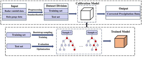
The RF-based fusion workflow comprises five key steps: data preparation, feature selection, model training, evaluation and optimization, and prediction, as illustrated in Figure 3. The model captures complex non-linear relationships and spatiotemporal dependencies by integrating multiple decision trees, yielding stable and accurate predictions. In this study, the geographical location of rain gauges and the rainfall time series were selected as predictor features. The number of decision trees was set to 100.

Figure 3. Workflow of the Random Forest algorithm for radar–gauge rainfall data fusion.

It is important to distinguish between two usage scenarios of the RF model in this study. For the independent accuracy assessment via leave-one-gauge-out cross-validation (Section 2.6.1), the RF model was trained on four gauges and validated on the withheld fifth gauge, with only the radar QPE, longitude, and latitude as predictor features. For the final fused rainfall products employed in the hydrological simulations (Section 3.4), the RF model was trained on all five gauges to provide the best possible areal rainfall estimates. This distinction ensures that the cross-validation metrics reflect genuine predictive skill at ungauged locations, while the final fused rainfall products for hydrological simulations were generated using all five gauges to provide the best possible areal rainfall estimates.

2.5. Hydrological Model Configuration

2.5.1. HEC-HMS Model Overview

The HEC-HMS (Hydrologic Engineering Center–Hydrologic Modeling System, version 4.3.0.0) hydrological model, developed by the Hydrologic Engineering Center of the U.S. Army Corps of Engineers, is a semi-distributed model known for its broad applicability, comprehensive functionality, and adaptability to diverse climatic environments, leading to widespread adoption internationally [56,57]. Model construction comprises four primary components: the basin module, meteorological module, control specifications module, and data storage module. Topographic preprocessing is facilitated through the HEC-GeoHMS extension within ArcGIS, while data storage and retrieval are managed via the HEC-DSSVue module, substantially streamlining model construction and data input tasks.

2.5.2. Runoff Generation and Flow Routing Methods

The HEC-HMS model partitions runoff process simulation into four computational modules: loss (calculation of rainfall losses and effective precipitation), direct runoff transformation, baseflow, and channel routing. For this study, the initial and constant loss method was selected for loss calculation, the Snyder unit hydrograph method for direct runoff transformation, the exponential recession method for baseflow estimation, and the Muskingum method for channel routing. These methods have demonstrated satisfactory performance in previous flood simulation studies [58,59,60]. The simulation time step was set to one hour.

The key parameters of these methods are: the constant loss rate (mm h⁻¹) in the initial and constant loss method; the peak flood lag time Tp (h) and the attenuation coefficient k in the Snyder unit hydrograph method; the flow proportion factor x (dimensionless) and the travel time K (h) in the Muskingum channel routing method.

2.6. Accuracy Evaluation Metrics

2.6.1. Leave-One-Gauge-Out Cross-Validation Strategy

To rigorously assess the predictive capability of the three fusion methods at ungauged locations, a leave-one-gauge-out cross-validation (LOOCV) procedure was implemented. Because GDA and CM act as exact interpolators at gauge locations—and RF can severely overfit when evaluated at the same points used for training—evaluating any of these methods at the training gauges leads to artificially inflated accuracy metrics. The LOOCV approach eliminates this data leakage by ensuring that the validation station is entirely excluded from the model-building process [61,62].

For each rainfall event, the following procedure was executed for each of the five rain gauges:

(1)

The target gauge is withheld as the validation station, and the remaining four gauges serve as the training set.

(2)

The fusion model (GDA, CM, or RF) is constructed using only the training gauges.

(3)

The model predicts the hourly precipitation at the location of the withheld gauge.

(4)

Steps 1–3 are repeated until each gauge has been withheld exactly once.

This yields, for each event and each fusion method, a set of independently predicted precipitation values at all five gauge locations. The accuracy metrics defined in Section 2.6.2 (CC, Bias, and RMSE) are then calculated using these independent predictions and the corresponding gauge observations. The LOOCV-based metrics thus reflect the true skill of each method in estimating precipitation at points not used during model training [63].

To ensure stable variogram estimation from the four training gauges during LOOCV, a climatological variogram was constructed for each training set by pooling all time steps within the event, following the same approach used for the full five-gauge interpolation [64].

It is important to note that the LOOCV procedure is used exclusively for independent accuracy assessment. The final fused rainfall products employed in the hydrological simulations (Section 3.4) are generated using all five gauges to provide the best possible areal rainfall estimates for model forcing.

2.6.2. Evaluation Metrics for Radar QPE and Fused Rainfall

Three metrics—Correlation Coefficient (CC), Bias, and Root Mean Square Error (RMSE)—were employed to evaluate radar QPE and fused rainfall product quality, as defined in Equations (10)–(12). CC quantifies the linear correlation between estimated/fused and observed values. A positive Bias indicates overestimation relative to observations, while a negative Bias indicates underestimation; values closer to zero denote smaller systematic deviation. A smaller RMSE corresponds to smaller estimation or fusion error.

$$CC={\displaystyle \frac{{\displaystyle {\sum }_{i=1}^N}\left(y_i-\overline{y_i}\right)\left(p_i-\overline{p_i}\right)}{\sqrt{{\displaystyle {\sum }_{i=1}^N}(y_i-\overline{y_i}{)}^2{\displaystyle {\sum }_{i=1}^N}(p_i-\overline{p_i}{)}^2}}}$$

(10)

$$Bias={\displaystyle \frac{1}{N}}{\displaystyle {\sum }_{i=1}^N}\left(y_i-p_i\right)$$

(11)

$$RMSE=\sqrt{{\displaystyle \frac{1}{N}}{\displaystyle \sum _{i=1}^N}(y_i-p_i{)}^2}$$

(12)

where y_i represents the radar-estimated or fused rainfall value, p_i is the corresponding gauge-observed rainfall, $\overline{*}$ denotes mean values, and N is the total number of samples.

2.6.3. Evaluation Metrics for Flood Simulation

Hydrological model performance was evaluated using Relative Error of Peak Discharge (RE_P), Relative Error of Runoff Volume (RE_V), Peak Time Error (ΔT), and Nash–Sutcliffe Efficiency Coefficient (NSE). REP and REV quantify the proportional deviation of simulated peak discharge and runoff volume from observed values Equations (13) and (14). ΔT measures the timing offset between simulated and observed flood peaks Equation (15). NSE assesses overall hydrograph agreement, with values closer to 1 indicating better fit Equation (16).

$$R{E}_P={\displaystyle \frac{Q_S-Q_O}{Q_O}}$$

(13)

$$R{E}_V={\displaystyle \frac{V_S-V_O}{V_O}}$$

(14)

$$∆T=T_s-T_O$$

(15)

$$NSE=1-{\displaystyle \frac{{\sum }_{i=1}^n{\left(Q_{O,i}-Q_{S,i}\right)}^2}{{\sum }_{i=1}^n{\left(Q_{O,i}-\overline{Q_O}\right)}^2}}$$

(16)

where $Q_O$ and $Q_S$ denote the observed and simulated peak discharges; $V_O$ and $V_S$ the observed and simulated runoff volume; $T_O$ and $T_s$ the observed and simulated times to peak; n the number of time steps; $Q_{O,i}$ and $Q_{S,i}$ denote the observed and simulated discharges at time step i; and $\overline{Q_O}$ the mean observed discharge.

3. Results

3.1. Radar Quantitative Precipitation Estimation Performance

The dynamically optimized Z-I relationship was applied to generate QPE for the five selected rainfall events. Table 1 summarizes the basin-scale areal rainfall accuracy of radar QPE, evaluated by comparing Thiessen-weighted radar areal rainfall against gauge-based areal rainfall at the five rain gauge stations. Consistently negative Bias values across all events confirm a systematic underestimation characteristic of the radar QPE (overall Bias = −2.83). The 20120726 event produced the poorest results, with a CC of 0.18, Bias of −5.27, and RMSE of 16.83. The method performed better for long-duration events with uneven rainfall distribution, with the best overall metrics among the five events recorded for the 20210721 event (CC = 0.53, RMSE = 6.31). Events characterized by short-duration, high-intensity rainfall (20120726 and 20230825) showed markedly lower retrieval accuracy. Additionally, the radar station was still a single-polarization system in 2012, and the echo data may have contained significant numerical errors, further contributing to the poor QPE performance for the 20120726 event.

Table 1. Basin-scale areal rainfall accuracy of radar QPE across the five typical rainfall events.

Metrics	20120726	20160719	20210721	20230730	20230825	Overall
CC	0.1784	0.3761	0.5280	0.3956	0.2127	0.3983
Bias	−5.27	−5.17	−2.00	−1.71	−1.97	−2.83
RMSE	16.83	10.85	6.31	5.87	8.95	8.65

Note: The areal rainfall is computed by applying Thiessen polygon weights to the radar QPE values at the five gauge locations. The “Overall” row aggregates all time steps from the five events to compute a single metric for QPE.

The considerably lower accuracy for short-duration, high-intensity events (20120726 and 20230825) can be attributed, in part, to a fundamental limitation of the dynamically optimized Z-I relationship. This method derives the optimal Z-I parameters from the preceding hour’s radar–gauge comparison and applies them to the current hour. For stratiform or long-duration rainfall, the microphysical properties of precipitation evolve gradually, and the previous hour’s Z-I relationship remains reasonably representative. However, for convective storms, precipitation characteristics can change abruptly: the hour preceding a sudden downpour may consist of weak, non-convective rainfall governed by a markedly different Z-I relationship, which, when applied to the subsequent intense rainfall, leads to significant estimation errors. This mismatch between the calibration window and the target hour is an inherent weakness of the hourly update strategy when applied to rapidly evolving convective systems.

3.2. Independent Validation of Radar–Gauge Rainfall Data Fusion Accuracy

The leave-one-gauge-out cross-validation (LOOCV) results for point-scale and basin-scale accuracy are presented in Table 2 and Table 3, respectively. These metrics reflect the true predictive capability of each fusion method at ungauged locations, free from the data leakage that occurs when evaluation is performed at the same gauges used for model training.

Table 2. Point-scale accuracy of fused rainfall under leave-one-gauge-out cross-validation (all five events combined).

Method	Gauge	CC	Bias	RMSE
GDA	Shentou	0.7358	−0.42	6.74
	Pusaling	0.8134	0.42	5.52
	Anshang	0.8092	−0.31	5.58
	Renzhuang	0.8665	0.55	4.97
	Liulin	0.8383	−0.15	5.68
	Overall	0.8115	0.02	5.73
CM	Shentou	0.7780	−0.62	6.18
	Pusaling	0.8027	0.20	5.64
	Anshang	0.8020	−0.31	5.69
	Renzhuang	0.8580	0.50	5.11
	Liulin	0.8309	−0.15	5.80
	Overall	0.8131	−0.08	5.69
RF	Shentou	0.4218	−1.02	8.90
	Pusaling	0.5723	0.66	7.90
	Anshang	0.5580	−0.17	7.75
	Renzhuang	0.2729	−0.08	10.09
	Liulin	0.5616	0.45	8.77
	Overall	0.4798	−0.03	8.72

Note: The “Overall” row is calculated by pooling all stations and all time steps across the five events.

Table 3. Basin-scale areal rainfall accuracy under leave-one-gauge-out cross-validation for each event.

Event	Method	CC	Bias	RMSE
20120726	QPE	0.1784	−5.27	16.83
	GDA	0.9997	0.26	0.52
	CM	0.9997	0.24	0.49
	RF	0.9086	−1.36	10.10
20160719	QPE	0.3761	−5.17	10.85
	GDA	0.8670	−0.14	5.02
	CM	0.8890	−0.57	4.65
	RF	0.5372	−0.64	8.52
20210721	QPE	0.5280	−2.00	6.31
	GDA	0.9918	−0.29	0.91
	CM	0.9865	−0.38	1.16
	RF	0.5877	−0.47	5.34
20230730	QPE	0.3956	−1.71	5.87
	GDA	0.9954	0.14	0.60
	CM	0.9950	0.14	0.63
	RF	0.4317	0.26	5.54
20230825	QPE	0.2127	−1.97	8.95
	GDA	0.9990	−0.08	0.97
	CM	0.9992	−0.07	0.89
	RF	0.2221	−0.47	8.90
Overall	QPE	0.3983	−2.83	8.65
	GDA	0.9596	−0.03	2.48
	CM	0.9644	−0.15	2.34
	RF	0.6193	−0.28	6.94

Note: The “Overall” row aggregates all time steps from the five events to compute a single metric for each method.

Point-scale accuracy (Table 2) reveals several important findings. First, the LOOCV evaluation yields overall CC values of 0.812 (GDA), 0.813 (CM), and 0.480 (RF), with corresponding RMSE values of 5.73 mm, 5.69 mm, and 8.72 mm, respectively. These LOOCV results reflect the true generalization capability of each method. By design, GDA and CM act as exact interpolators at gauge locations and would yield artificially high metrics if evaluated at the training gauges; similarly, RF is prone to overfitting when assessed on its training samples. The LOOCV procedure eliminates this source of inflation, and the values reported here therefore represent the genuine predictive skill at ungauged locations. Second, GDA and CM exhibited very similar and markedly better point-scale performance than RF. Their per-station CC ranged from 0.736 to 0.867 (GDA) and 0.778 to 0.858 (CM), whereas RF achieved CC values between only 0.273 and 0.572. This indicates that the geostatistical methods, which exploit the spatial covariance structure of the radar rainfall field, generalize more robustly to ungauged points than the purely data-driven RF model when trained with only four spatial samples. Third, station-specific accuracy varied considerably. For GDA, the best-predicted station was Renzhuang (CC = 0.867), followed by Pusaling (CC = 0.813). For CM, Renzhuang (CC = 0.858) and Pusaling (CC = 0.803) showed similarly good performance. For RF, Renzhuang was the worst-predicted station (CC = 0.273), indicating severe spatial overfitting.

Basin-scale areal rainfall accuracy (Table 3) demonstrates a striking contrast with point-scale results. Despite the moderate point-scale errors, the area-weighted basin-average rainfall derived from GDA and CM maintained very high fidelity. For GDA, per-event basin CC ranged from 0.867 to 0.999, and the overall basin CC across all five events reached 0.960, with an overall RMSE of only 2.48 mm. CM performed comparably, with an overall basin CC of 0.964 and RMSE of 2.34 mm. This robustness arises from spatial error cancellation: the positive and negative prediction errors at individual gauge locations largely offset each other during area-weighted averaging. In contrast, RF produced markedly inferior basin-scale estimates, with per-event CC values as low as 0.222 (Event 20230825) and an overall basin CC of only 0.619. The poor spatial generalization of RF, already evident at the point scale, propagates directly into unreliable areal rainfall estimates.

The divergence between the near-perfect in-sample fit and the considerably lower independent accuracy underscores the necessity of rigorous cross-validation when evaluating rainfall fusion methods. Under LOOCV, GDA and CM exhibit genuinely higher predictive skill than RF at both point and areal scales. GDA’s superior generalization directly accounts for its most robust flood simulation performance. For CM, although its statistical accuracy was comparable to GDA, its flood simulation results were slightly inferior to those of RF, indicating that additional factors—such as the spatial smoothness of the correction field—may modulate the translation from rainfall accuracy to hydrological skill. This finding highlights that while robust spatial generalization (as demonstrated by GDA and CM) is essential for reliable areal rainfall estimation, the translation from rainfall accuracy to hydrological performance can be modulated by additional factors such as the spatial characteristics of the fused rainfall field. Detailed per-event, per-station point-scale metrics from the LOOCV are provided in Appendix A Table A1 for completeness.

3.3. HEC-HMS Model Calibration and Validation

3.3.1. Parameter Optimization

The 1 m resolution DEM was processed using HEC-GeoHMS 10.2 in ArcGIS 10.2, yielding a delineation of nine sub-basins (Figure 4). The nine delineated sub-basins are labeled W100 to W180, and the four channel reaches are labeled R50 to R80. Gauge-based point rainfall was converted to areal rainfall via the Thiessen polygon method and assigned to corresponding sub-basins as weighted rainfall input.

Figure 4. Results of sub-basin delineation.

Among the 22 selected rainfall-runoff events (1995–2023), 12 events from 1995 to 2003 served for calibration, and 10 events from 2004 to 2023 for validation. Parameter calibration employed the Univariate-Gradient automatic optimization algorithm within HEC-HMS, using the Peak-Weighted Root Mean Square Error (PRMSE) as the objective function—a choice motivated by its demonstrated advantages in previous studies [65,66].

Automatically optimized parameters were subsequently refined manually to ensure physical consistency with watershed characteristics. The calibrated channel routing parameters (Muskingum x and K) are presented in Table 4, and the sub-basin loss and transform parameters (constant loss rate, Snyder Tp and k) are presented in Table 5.

Table 4. Calibrated parameters for channel reaches.

Parameter	Range	R50	R60	R70	R80
x	0~0.5	0.31	0.23	0.12	0.27
K	0.1~150 h	0.83	0.10	0.35	0.10

Note: x = flow proportion factor (dimensionless) in the Muskingum routing method; K = travel time (h) in the Muskingum routing method. Parameters are calibrated for each channel reach (R50–R80).

Table 5. Calibrated parameters for sub-basins.

Parameter	W180	W170	W160	W150	W140	W130	W120	W110	W100
Constant loss rate	0.77	0.31	0.23	0.22	0.39	0.26	0.25	0.25	0.23
Tp	0.75	0.73	0.74	0.73	0.74	0.74	0.76	0.76	0.75
k	0.04	0.03	0.02	0.04	0.02	0.04	0.02	0.02	0.02

Note: Constant loss rate (mm h⁻¹) is the loss parameter in the initial and constant loss method; Tp = peak flood lag time (h) in the Snyder unit hydrograph method; k = attenuation coefficient in the Snyder unit hydrograph method. Parameters are calibrated for each sub-basin (W100–W180).

3.3.2. Flood Simulation Performance

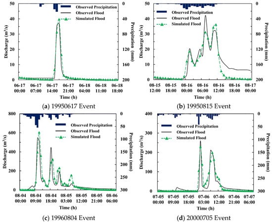
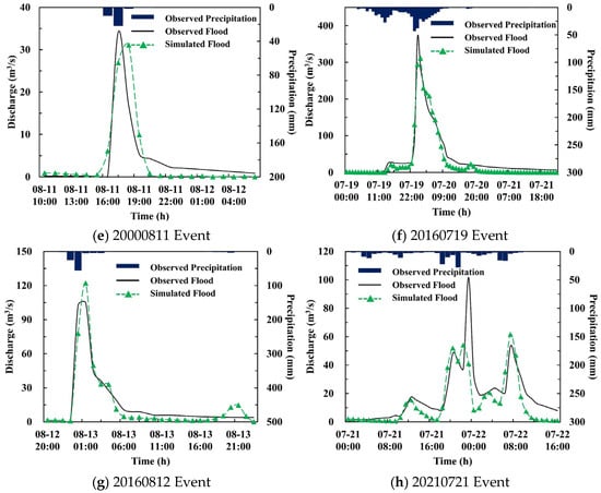
Table 6 and Figure 5 present the calibration and validation results. For the 12 calibration events, the mean absolute RE_P was 17.57%, mean RE_V 14.06%, mean ΔT 0.75 h, and mean NSE 0.72—meeting the “Good” accuracy grade (0.36 < NSE < 0.75) as defined by Krause et al. [67]. For the 10 validation events, the corresponding metrics were mean RE_P 22.88%, mean RE_V 16.50%, mean ΔT 1.3 h, and mean NSE 0.69. These results confirm the applicability of the constructed HEC-HMS model to the Liulin watershed.

Table 6. Flood simulation results for calibration and validation periods.

Period	Events	Qo m3/s	Vo mm	Qs m3/s	REP %	Vs mm	REV %	ΔT h	NSE
Calibration	19950617	37.00	6.88	39.70	7.30	7.53	9.45	0.0	0.95
	19950713	27.90	5.48	28.10	0.72	4.95	−9.67	2.0	0.50
	19950714	103.00	11.36	63.80	−38.06	11.11	−2.20	0.0	0.75
	19950815	42.10	23.08	36.20	−14.01	18.70	−18.98	4.0	0.80
	19960716	15.70	2.30	14.80	−5.73	2.70	17.39	0.0	0.73
	19960804	543.00	225.04	603.70	11.18	255.70	13.62	1.0	0.73
	19960821	53.20	8.58	51.40	−3.38	6.90	−19.58	0.0	0.98
	19980718	15.80	1.78	11.90	−24.68	1.80	1.12	0.0	0.81
	19980814	30.30	2.66	16.90	−44.22	3.48	30.83	0.0	0.55
	20000705	260.00	90.75	229.10	−11.88	97.01	6.90	0.0	0.79
	20000811	34.10	5.01	31.10	−8.80	5.06	1.00	1.0	0.71
	20030916	33.30	4.85	19.70	−40.84	3.01	−37.94	1.0	0.30
Absolute mean value					17.57		14.06	0.75	0.72
Validation	20040729	32.70	4.20	27.40	−16.21	4.07	−3.10	1.0	0.80
	20040812	124.90	35.36	137.90	−8.68	35.30	−0.17	0.0	0.58
	20060813	65.30	10.39	61.80	−5.36	12.08	16.27	1.0	0.81
	20120726	47.00	7.37	33.40	−28.94	7.73	4.88	0.0	0.65
	20160719	368.00	147.01	311.60	−15.33	142.70	−18.50	1.0	0.94
	20160807	48.10	11.91	30.00	−37.63	6.90	−42.07	1.0	0.55
	20160812	105.00	28.93	122.10	16.29	26.29	−9.13	0.0	0.93
	20210721	101.80	47.65	61.60	−39.49	36.16	−24.11	8.0	0.55
	20230730	111.00	75.06	94.90	−14.50	57.16	−23.85	0.0	0.66
	20230825	85.50	12.87	45.80	−46.43	7.92	−38.46	1.0	0.47
Absolute mean value					22.88		16.50	1.30	0.69

Figure 5. Simulation results of flood hydrographs for selected events.

Nonetheless, the model exhibited limitations in peak discharge simulation. Among all 22 events, only 14 achieved RE_P below 20%, consistent with the performance range reported for HEC-HMS in similar contexts [59,68]. Significant peak flow biases occurred primarily under two scenarios: short-duration, high-intensity events with low antecedent soil moisture (e.g., 19980814, 20030916), where infiltration-excess runoff dominates, and the model inadequately represents localized hydrological responses such as depression storage and vegetation interception; and long-duration events with uneven rainfall distribution (e.g., 20210721), where infiltration-excess and saturation-excess mechanisms coexist and dynamically interact, enhancing rainfall-runoff nonlinearity and simulation uncertainty.

3.4. Flood Simulation with Multi-Source Rainfall Inputs

The five flood events were simulated using the HEC-HMS model driven by five distinct rainfall inputs: gauge-measured rainfall, radar-only QPE, and fused data from GDA, CM, and RF. Quantitative evaluation metrics are presented in Table 7.

Table 7. Flood simulation evaluation metrics under different rainfall inputs.

Event	Source	REP %	REV %	ΔT h	NSE
20120726	Gauge	−28.94	4.88	0	0.651
	QPE	−97.87	−93.04	−7	−0.278
	GDA	−17.66	8.61	0	0.799
	CM	−17.87	9.71	0	0.793
	RF	−15.53	20.33	0	0.748
20160719	Gauge	−15.33	−2.93	1	0.942
	QPE	−92.80	−88.76	−8	−0.302
	GDA	−5.84	−1.44	1	0.943
	CM	−6.39	−1.85	1	0.943
	RF	−7.80	−0.22	1	0.938
20210721	Gauge	−39.49	−24.11	8	0.550
	QPE	−31.53	−51.86	0	0.336
	GDA	−24.17	−13.87	0	0.858
	CM	−27.60	−14.35	0	0.844
	RF	−38.21	−21.11	0	0.806
20230730	Gauge	−14.50	−23.85	0	0.656
	QPE	−45.14	−72.22	−11	−0.845
	GDA	−8.74	−11.38	0	0.695
	CM	−7.93	−13.03	0	0.698
	RF	−4.77	−7.34	0	0.717
20230825	Gauge	−46.43	−38.46	1	0.471
	QPE	−77.89	−61.07	2	0.103
	GDA	−39.42	−20.05	1	0.657
	CM	−39.53	−20.44	1	0.656
	RF	−32.40	−21.68	0	0.685

Radar-only QPE produced the poorest performance across all events, with peak discharges and runoff volumes severely underestimated and NSE values typically below zero, reflecting the systematic underestimation inherent in uncorrected radar estimates.

For the 20120726 event (a small-magnitude, single-peak flood induced by short-duration heavy rainfall), all rainfall inputs except radar data yielded satisfactory simulations. The GDA and CM fused data performed best, achieving NSE values of 0.799 and 0.793, respectively, with errors in both peak discharge and runoff volume below 20%. RF-fused data yielded an NSE of 0.748, with peak discharge error outperforming gauge data but runoff volume error slightly elevated.

For the 20160719 event (a large-magnitude, single-peak flood from continuous uniform rainfall), simulations using all non-radar inputs performed excellently, with NSE values above 0.9 and errors below 20% for both peak discharge and runoff volume. GDA fused data achieved the smallest peak discharge error (−5.84%), while RF data produced the smallest runoff volume error (−0.22%). GDA and CM shared the highest NSE (0.943), demonstrating the strong suitability of fused data for this flood type.

For the 20210721 event (a multi-peak flood from prolonged, non-uniform rainfall), all rainfall inputs exhibited peak discharge errors exceeding 20%, and gauge data showed an 8 h peak time error. Nevertheless, fused products significantly outperformed single-source data in hydrograph fitting: NSE values for GDA, CM, and RF were 0.858, 0.844, and 0.806, respectively, versus 0.550 (gauge) and 0.336 (radar). GDA and CM also produced smaller peak discharge and runoff volume errors.

For the 20230730 event, all non-radar inputs accurately captured the peak timing, with peak discharge errors below 20%. RF fused data performed best, achieving a peak discharge error of −4.77%, runoff volume error of −7.34%, and NSE of 0.717. Although RF achieved the best metrics among all inputs for this event, its NSE of 0.717 remained moderate, suggesting that even the best-performing fusion product faced challenges in fully capturing the rainfall-runoff dynamics of this multi-peak event.

For the 20230825 event, overall simulation performance was moderate across all inputs, with both peak discharge and runoff volume errors exceeding 20%. However, the three fused datasets still outperformed gauge and radar data. RF fused data accurately reproduced the peak timing, while GDA and CM showed a 1 h bias. NSE values for RF, GDA, and CM were 0.685, 0.657, and 0.656, respectively, clearly exceeding those for gauge data (0.471) and radar data (0.103).

4. Discussion

4.1. Quantitative Accuracy of Fused Rainfall Products

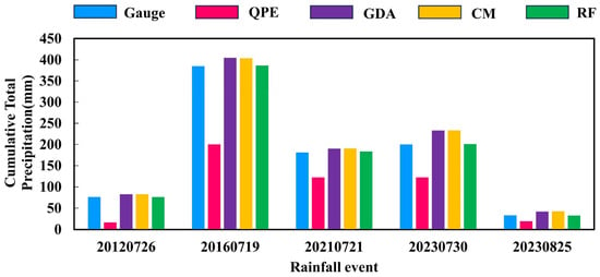
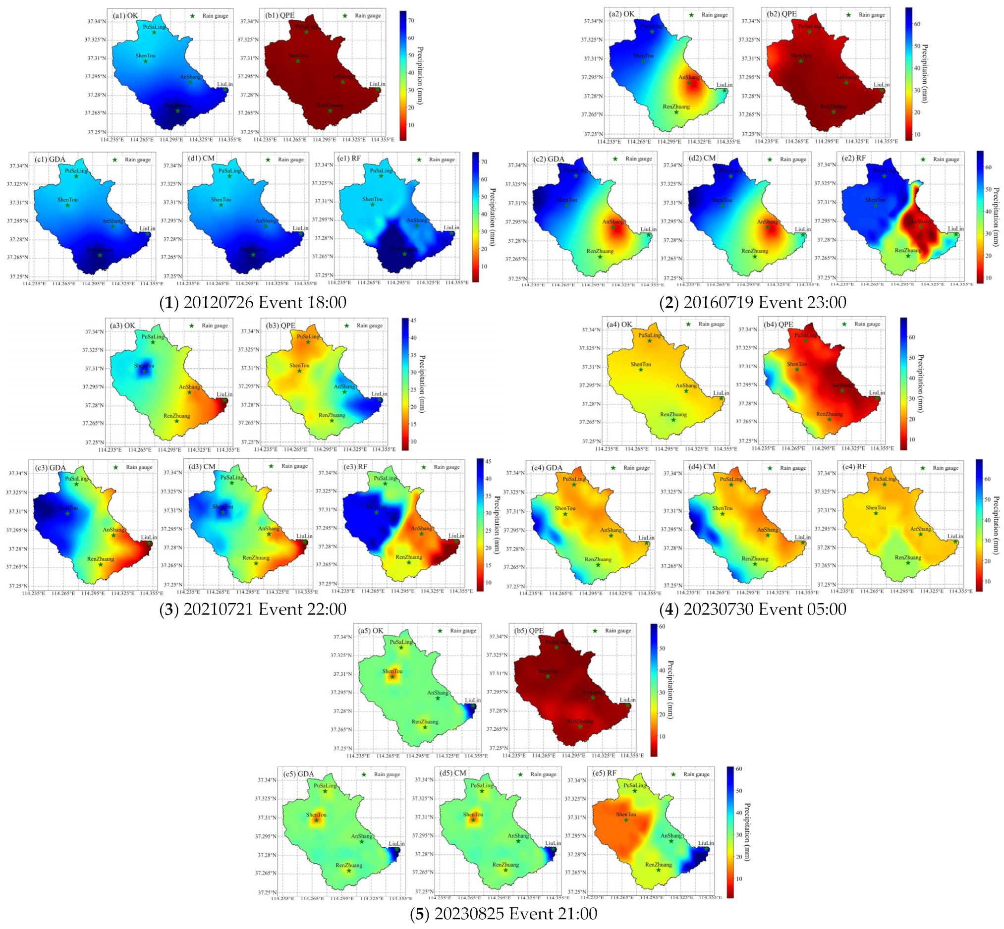
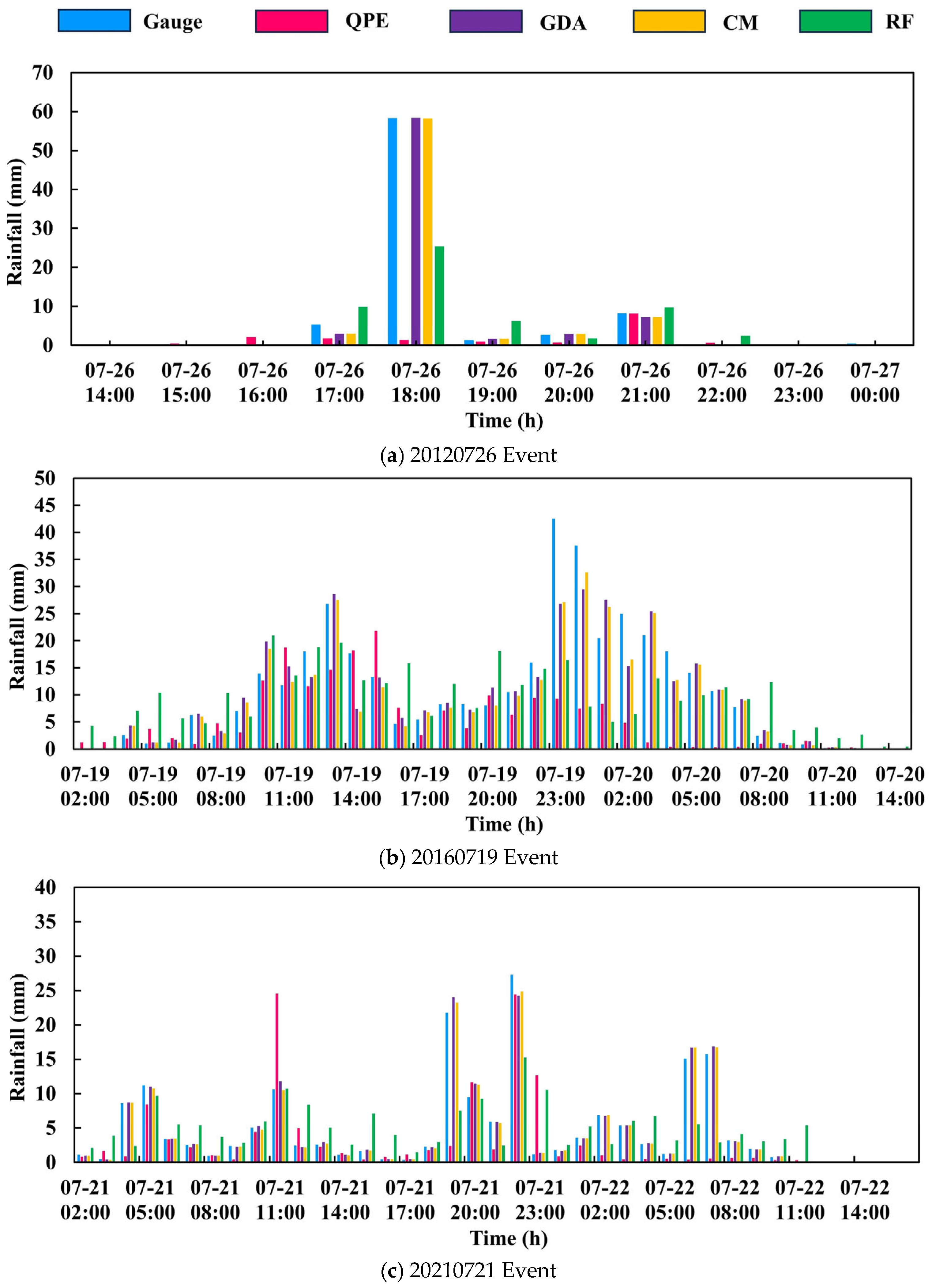
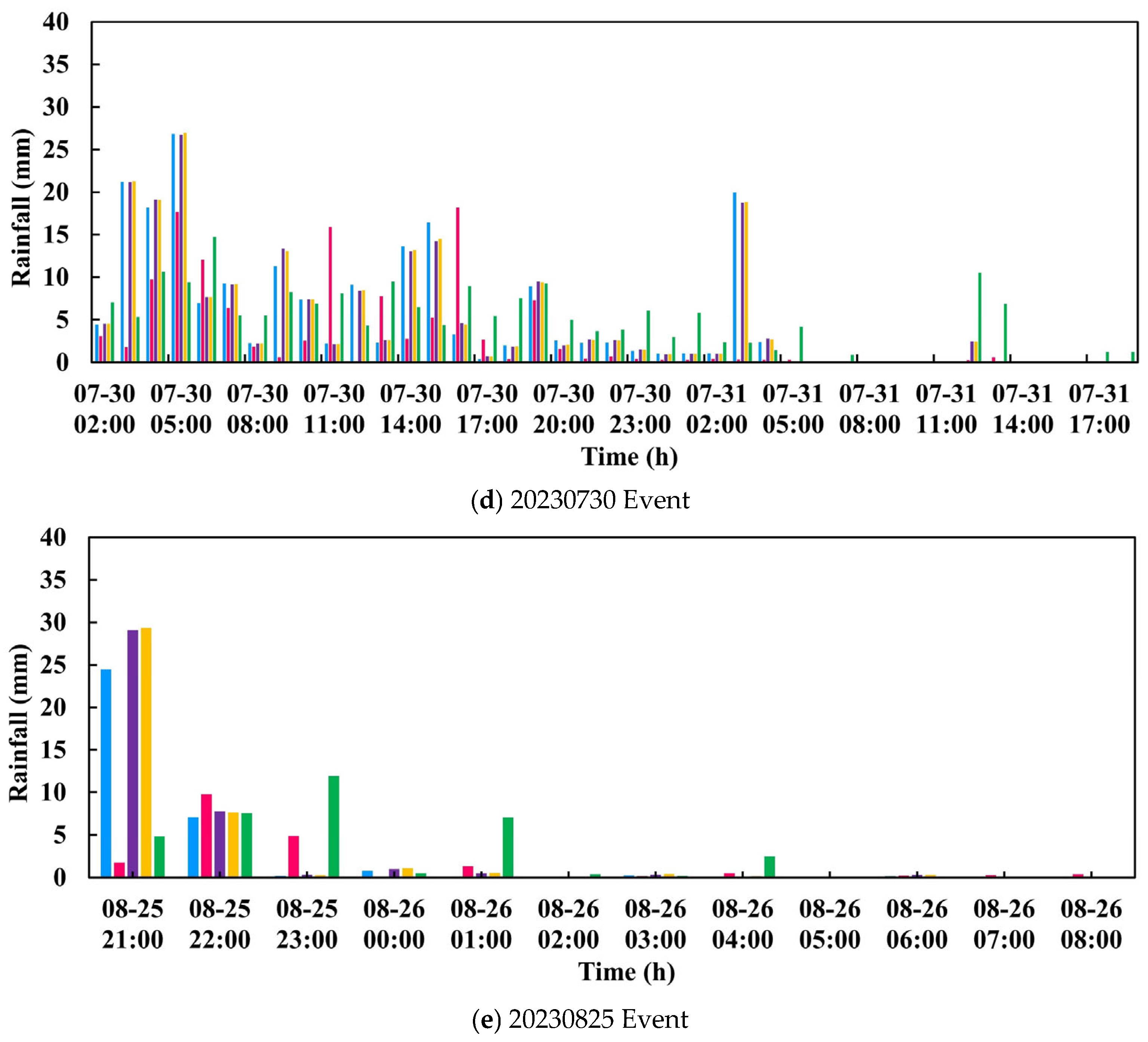
Table 8 and Figure 6 compare the cumulative event total rainfall from the five data sources. All three fusion methods effectively corrected the severe underestimation inherent in radar-only QPE, bringing the event totals much closer to the gauge observations. The RF estimates matched the gauge totals most closely (e.g., 75.94 mm vs. 76.34 mm for Event 20120726), which is expected given the method’s strong point-wise fitting capability when all gauges are used for training. However, as demonstrated by the independent LOOCV evaluation (Section 3.2), this agreement at the gauge locations does not guarantee reliable rainfall estimates between gauges.

Table 8. Cumulative total rainfall by event and data source (mm).

Event	Gauge	QPE	GDA	CM	RF
20120726	76.34	16.55	82.76	82.93	75.94
20160719	385.03	200.28	404.75	403.36	386.16
20210721	181.28	122.13	190.28	190.89	183.47
20230730	200.17	122.25	233.15	233.32	201.26
20230825	33.00	19.40	42.46	42.48	32.85

Figure 6. Comparison of cumulative total rainfall for the five events.

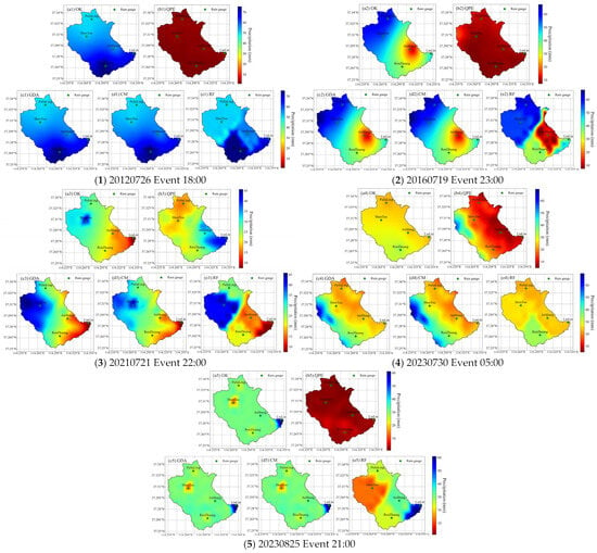
The spatial distribution maps of maximum 1 h rainfall (Figure 7) illustrate the characteristic behaviors of each method. All fused products capture considerably more spatial detail than the gauge-only Kriging interpolation, benefiting from the broad coverage of radar. GDA and CM preserve the fine-scale spatial variability inherent in the radar field, while RF produces noticeably smoother maps. This smoothness reflects RF’s reliance on point-based feature mapping without an explicit model of spatial covariance. Although visually acceptable at gauge sites, the LOOCV results indicate that such smooth fields can contain substantial spatial distortions in ungauged areas, which explains why RF, despite its competitive performance in certain events, was less robust overall than GDA in the flood simulations.

Figure 7. Spatial distribution maps of areal rainfall using fused data.

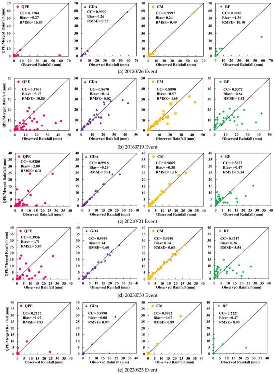
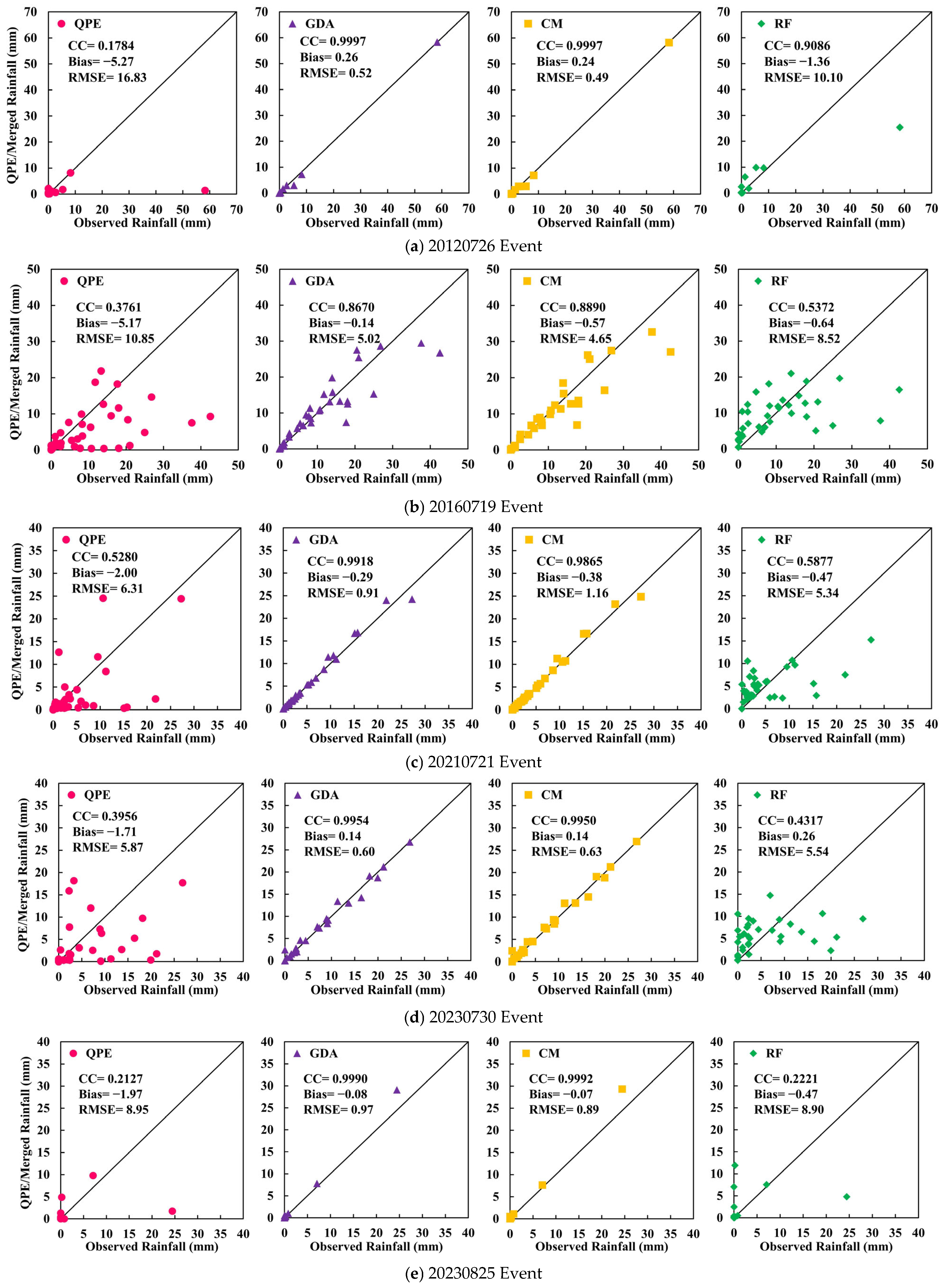
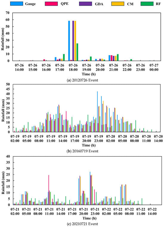
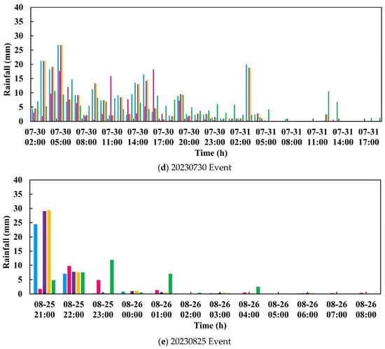
Scatter plots and hyetographs based on the LOOCV predictions (Figure 8 and Figure 9, respectively) further confirm these findings. The GDA and CM predictions remain clustered around the 1:1 line, albeit with increased scatter relative to the in-sample evaluation, while RF exhibits considerably larger deviations. Similarly, the LOOCV hyetographs show that GDA and CM track the temporal evolution of observed rainfall more faithfully, whereas RF displays marked departures during specific periods. These independent validation results demonstrate that the near-perfect point-scale accuracy that would be obtained by evaluating at the training gauges does not reflect true predictive skill. Moreover, they show that GDA—which, together with CM, demonstrated strong generalization under cross-validation—produces the most reliable areal rainfall estimates and the most robust flood simulations.

Figure 8. Scatter plots of fused rainfall versus observed rainfall.

Figure 9. Hyetographs for the typical rainfall events.

4.2. Accuracy Analysis of Flood Simulation Using Multi-Source Rainfall Data

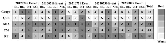
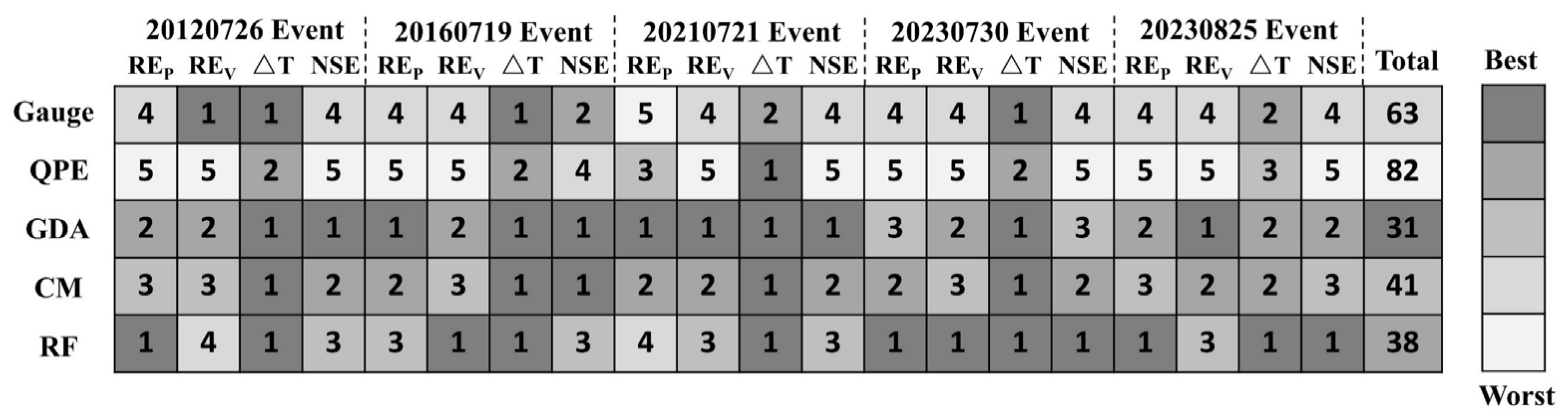
A comprehensive scoring system ranked the five rainfall inputs across all evaluation metrics (RE_P, RE_V, ΔT, NSE) for all events. The best-performing method received 1 point per metric per event, and the worst received 5 points. Lower total scores indicate superior overall flood simulation performance.

Figure 10 presents the aggregated scores: GDA achieved the best flood simulation performance (total score 31), followed by RF (38), CM (41), gauge-only (63), and radar-only (82). All three fused products consistently outperformed single-source rainfall data, confirming that fusion more accurately captures the true spatiotemporal distribution of watershed precipitation.

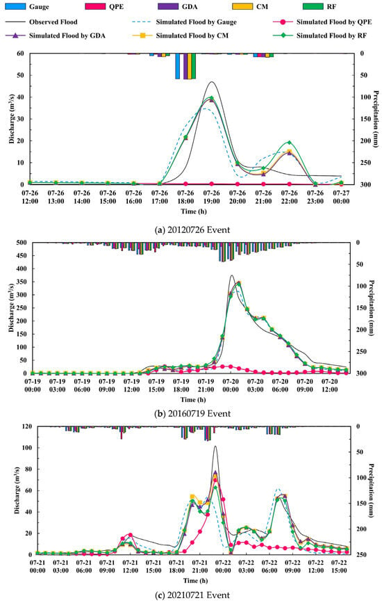
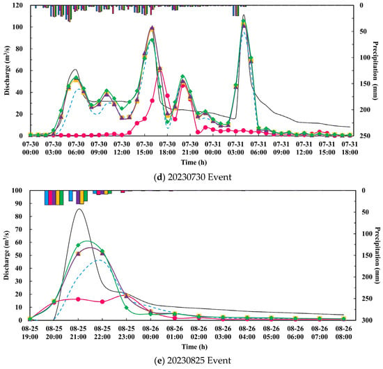
Figure 10. Comparative chart of flood simulation evaluation metric results.

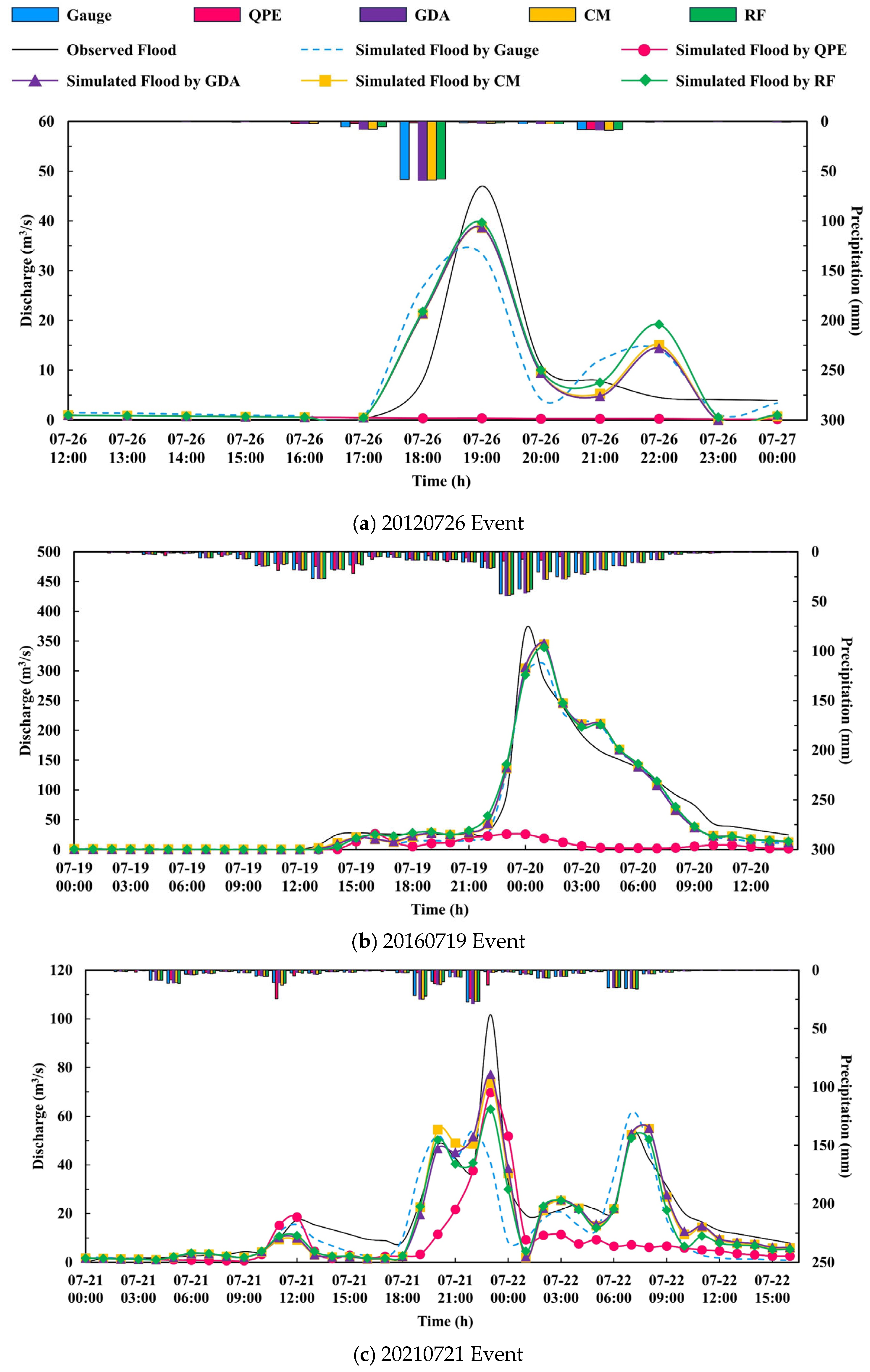
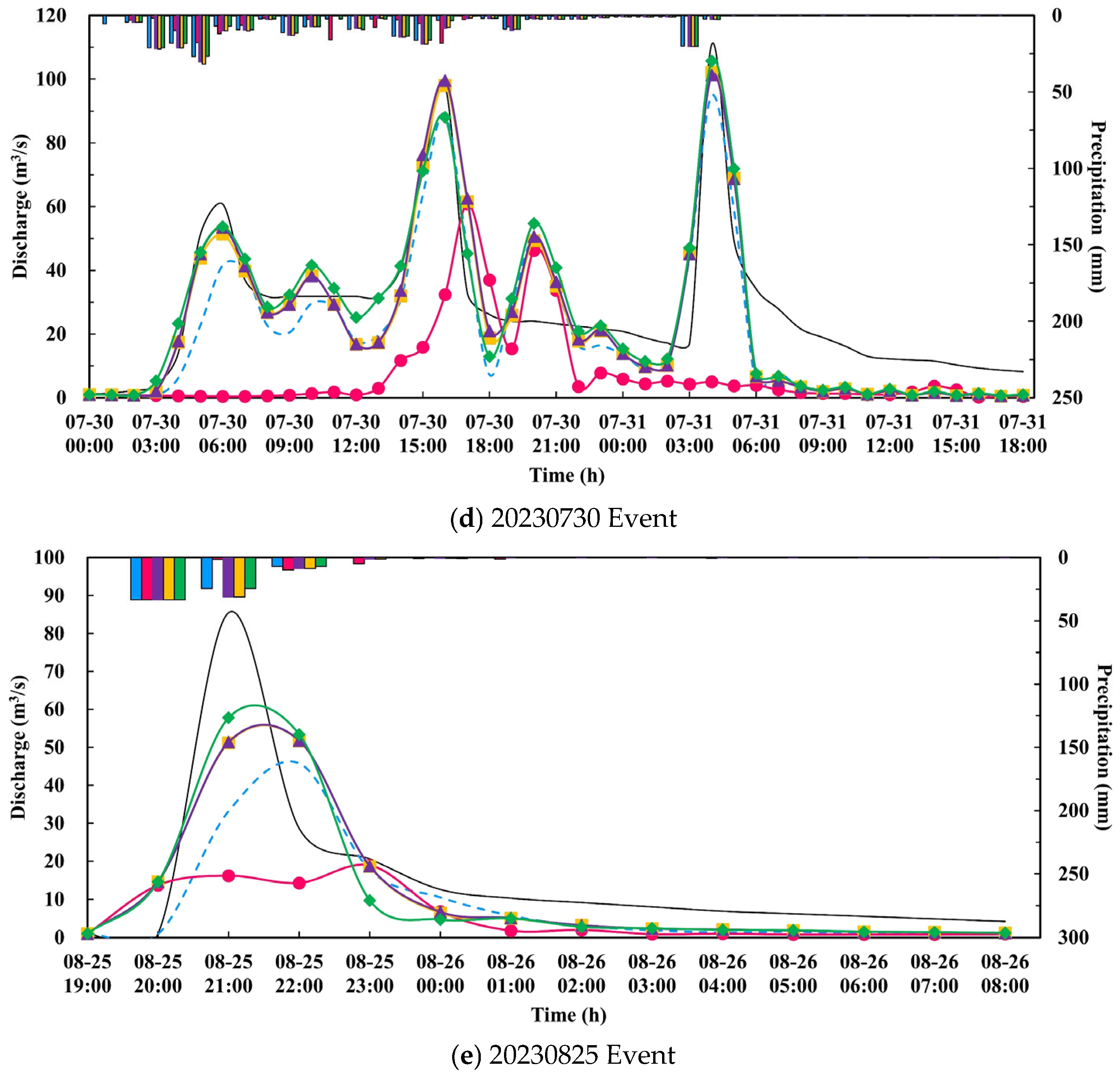
The flood simulation ranking is broadly consistent with the independent validation results. GDA, which achieved high point-scale (CC ≈ 0.81) and areal (CC ≈ 0.96) accuracy under LOOCV, delivered the most robust flood simulations. RF, despite its lower generalization (point CC ≈ 0.48, areal CC ≈ 0.62), ranked second in flood simulation performance, ahead of CM and the single-source inputs. This suggests that while independent cross-validation is essential for assessing true predictive skill, the relationship between statistical accuracy and hydrological utility is not strictly monotonic: RF’s basin-scale accuracy, though substantially lower than that of GDA and CM under LOOCV, was still sufficient to drive reasonably accurate flood simulations in several events. The flood hydrographs (Figure 11) further illustrate this: radar-only simulations failed to reproduce the rising and falling limbs, with some approaching a flat line. In contrast, all fused products and gauge data reasonably captured flood dynamics, though GDA and CM better represented recession limbs in multi-peak events compared to RF visually.

Figure 11. Flood hydrograph simulations with multi-source rainfall inputs.

For multi-peak events (20210721, 20230730), all non-radar inputs captured the rising limbs adequately but systematically underestimated recession limbs, likely attributable to the initial and constant loss method being inherently better suited to flashy, single-peak responses, and to limitations in baseflow parameter calibration. The 20230825 event exhibited generally poor performance across all inputs, with only the RF product accurately reproducing the peak timing.

4.3. Limitations and Future Research

This study has demonstrated the effectiveness of radar–gauge data fusion in enhancing flood simulation capability. However, several limitations warrant discussion.

(1) Although the 3 km CAPPI mitigates low-level beam blockage, it represents the reflectivity well above the ground, which may differ from the near-surface rainfall rate, especially in shallow convective systems or during stratiform precipitation with a bright band near the melting level [24]. Additionally, no dedicated fuzzy-logic clutter identification [69] or DEM-based beam blockage correction [70] was applied. Future studies could benefit from incorporating these advanced quality-control modules to further reduce residual non-meteorological echoes and range-dependent biases.

(2) The accuracy of radar QPE was relatively low for short-duration, high-intensity events, attributable to the inherent limitations of single-polarization radar in resolving convective precipitation microphysics and potential systematic errors in the radar base data [71]. Future work could employ multi-radar joint estimation and dual-polarization variables to improve retrieval stability. Additionally, the dynamically optimized Z-I relationship relies on the assumption that the microphysical properties of precipitation remain sufficiently stable between consecutive hours. As discussed in Section 3.1, this assumption breaks down during the rapid transitions characteristic of convective initiation, contributing to the poor QPE performance observed for short-duration, high-intensity events. Future implementations could explore sub-hourly updating strategies using real-time rain–gauge telemetry, or incorporate storm-type classification to apply distinct Z-I relationships for convective and stratiform precipitation regimes.

(3) Furthermore, the radar QPE relies on instantaneous intensity estimates at 6 min intervals to represent the continuous rainfall process within each hour. This discrete temporal sampling implicitly assumes that the instantaneous rainfall intensity observed at each scan is representative of the entire interval assigned to that scan (i.e., a piecewise-constant approximation), which may not hold during highly convective, pulsating precipitation. Sub-scan-scale fluctuations in rainfall intensity can lead to either overestimation or underestimation of the true hourly accumulation. This limitation is inherent to all radar QPE products derived from scanning radars with finite revisit times, and its impact is most pronounced for short-duration, high-intensity convective events. Future studies could explore fusion with higher-frequency observations, such as those from tipping-bucket rain gauges with sub-minute logging, to better resolve the sub-scan temporal variability [72].

(4) The Ordinary Kriging interpolation within GDA and CM relied on only five rain gauges per event. Although this represents a high-density network for a 57.4 km² basin, the 10 station pairs available per time step are below the sample size typically recommended for reliable variogram estimation. The climatological variogram approach adopted in this study mitigates this issue by pooling all time steps within each event, but it assumes temporal stationarity of the spatial structure, which may not hold during rapidly evolving convective systems [73]. The station-dependent LOOCV errors observed in Table 2, particularly the larger RMSE at Liulin, may partly reflect the sensitivity of the Kriging weights to variogram uncertainty. Future studies in similarly gauged basins could explore alternative spatial interpolation methods less reliant on variogram estimation, or incorporate external covariates such as elevation and radar-derived spatial metrics to constrain the interpolation.

(5) The RF method showed limited spatial generalization under independent cross-validation (point CC ≈ 0.48, areal CC ≈ 0.62). This indicates that RF, relying solely on static spatial and temporal features without an explicit spatial covariance model, has limited capacity to capture the spatiotemporal dynamics of evolving precipitation fields [74]. Nonetheless, its flood simulation performance ranked second among the three fusion methods, suggesting that even a moderately generalizable machine-learning fusion can retain practical utility for hydrological forecasting. Subsequent research should explore spatiotemporal deep learning architectures—such as integrating Convolutional Neural Networks (CNNs) with Long Short-Term Memory (LSTM) networks—to jointly model spatial patterns and their temporal evolution [19]. Hybrid models that combine the structural strengths of geostatistical methods with the non-linear mapping capability of machine learning also represent a promising direction.

(6) The uncertainty contributions from hydrological model parameters were not rigorously quantified in this study. A formal uncertainty analysis framework would disentangle the interacting effects of rainfall input error, parameter uncertainty, and model structural error, providing deeper insight into the predictive value of fused rainfall data [19].

5. Conclusions

This study systematically evaluated the chain from radar QPE generation, through multi-source rainfall data fusion, to flood simulation in a flash-flood-prone semi-arid watershed. The principal findings are as follows:

(1)

The dynamically optimized Z-I relationship provides a flexible framework for radar rainfall estimation, performing adequately for long-duration uniform events but showing limited skill for short-duration, high-intensity convective storms. Radar-derived rainfall exhibited a systematic underestimation bias, though its spatial structure was significantly more detailed than gauge-only interpolations.

(2)

All three fusion methods—GDA, CM, and RF—substantially improved rainfall data quality and corrected the systematic underestimation in radar QPE. Under independent cross-validation, GDA and CM yielded comparable point-scale accuracy (overall CC ≈ 0.81), with CM achieving slightly higher basin-scale accuracy (areal CC ≈ 0.964 vs. 0.960 for GDA), while RF exhibited markedly lower generalization (point CC ≈ 0.48, areal CC ≈ 0.62). Among the three, GDA and CM most effectively combined the high accuracy of gauge measurements with the high spatial resolution of radar.

(3)

In flood simulation, radar-only QPE produced the poorest results, with severe underestimation of peak discharge and runoff volume. Gauge-corrected fused rainfall significantly enhanced simulation accuracy and consistently outperformed any single-source data across diverse flood types. Among the fusion methods, GDA achieved the most robust overall flood simulation performance, followed by RF and CM. While differences among the three methods were not substantial, their collective superiority over single-source inputs confirms that radar–gauge data fusion provides a reliable and effective technical pathway for improving operational flood forecasting.

References

- Cheng, X.T.; Liu, C.J.; Li, C.Z.; Yu, Q.; Li, N. Evolution characteristics of flood risk under changing environment and strategy of urban resilience improvement. J. Hydraul. Eng. 2022, 53, 757–768. [Google Scholar] [CrossRef]
- Gu, W.; Chen, L.-J.; Wang, Y.-G.; Gao, H.; Wang, L.; Liu, Y.-Y. Extreme precipitation over northern China in autumn 2021 and joint contributions of tropical and mid-latitude factors. Adv. Clim. Change Res. 2022, 13, 835–842. [Google Scholar] [CrossRef] [Scilit]
- Ma, Q.; Li, Z.M.; Dong, F.R.; Zhang, K.; Yang, B.; Liu, C. Flood modeling developed for digital twin watershed: A case study of “23·7” great flood assessment in Ziya River Basin. J. Hydraul. Eng. 2025, 56, 73–84. [Google Scholar] [CrossRef]
- Duan, R.; Huang, G.; Zhou, X.; Lu, C.; Tian, C. Record-breaking heavy rainfall around Henan Province in 2021 and future projection of extreme conditions under climate change. J. Hydrol. 2023, 625, 130102. [Google Scholar] [CrossRef] [Scilit]
- Yuan, X.M.; Li, D.; Tian, F.C.; He, X.; Wang, X.; Guo, L. Research on flood classified intelligent forecasting method based on AE-RCNN. J. Hydraul. Eng. 2023, 54, 1070–1079. [Google Scholar] [CrossRef]
- Liu, W.; Xie, S.; Zhong, D.Y.; Wang, Y.; Bao, S.; Zhu, X. Coupled forecasting of rainstorms and floods in small watershed based on Deep Learning and HEC-HMS Model. J. Hydraul. Eng. 2025, 56, 364–374. [Google Scholar] [CrossRef]
- Liu, J.; Qiu, Q.T.; Li, C.Z.; Jiao, Y.; Wang, W.; Yu, F. Advances of precipitation nowcasting and its application in hydrological forecasting. Adv. Water Sci. 2020, 31, 129–142. [Google Scholar] [CrossRef]
- Zheng, Y.C.; Li, J.Z.; Rong, Y.T.; Du, Y.; Feng, P. Quantification of rainfall spatial and temporal distribution characteristics on the flood hydrograph and its application in flood type classification. J. Hydraul. Eng. 2022, 53, 560–573. [Google Scholar] [CrossRef]
- Li, Z.; Yang, D.W.; Hong, Y.; Qi, Y. Radar-based quantitative precipitation estimate in the Three Gorges region of Yangtze River. J. Hydraul. Eng. 2014, 33, 29–54. [Google Scholar]
- Renard, B.; Kavetski, D.; Kuczera, G.; Thyer, M.; Franks, S.W. Understanding predictive uncertainty in hydrologic modeling: The challenge of identifying input and structural errors. Water Resour. Res. 2010, 46, W05521. [Google Scholar] [CrossRef] [Scilit]
- Liu, X.Y.; Diallo, T.D.; Mao, J.T.; Li, J. Monthly Precipitation Estimation over Western China Using GMS Satellite Data. Chin. J. Atmos. Sci. 2005, 29, 518–525. [Google Scholar]
- Smith, J.A.; Baeck, M.L.; Zhang, Y.; Doswell, C.A. Extreme rainfall and flooding from supercell thunderstorms. J. Hydrometeorol. 2001, 2, 469–489. [Google Scholar] [CrossRef] [Scilit]
- Hazenberg, P.; Leijnse, H.; Uijlenhoet, R. Radar rainfall estimation of stratiform winter precipitation in the Belgian Ardennes. Water Resour. Res. 2011, 47, W02507. [Google Scholar] [CrossRef] [Scilit]
- He, X.; Refsgaard, J.C.; Sonnenborg, T.O.; Vejen, F.; Jensen, K.H. Statistical Analysis of the Impact of Radar Rainfall Uncertainties on Water Resources Modeling: Radar Rainfall Uncertainties on Hydrological Modeling. Water Resour. Res. 2011, 47, W09526. [Google Scholar] [CrossRef] [Scilit]
- Chang, W.-Y.; Vivekanandan, J.; Ikeda, K.; Lin, P.-L. Quantitative Precipitation Estimation of the Epic 2013 Colorado Flood Event: Polarization Radar-Based Variational Scheme. J. Appl. Meteorol. Climatol. 2016, 55, 1477–1495. [Google Scholar] [CrossRef] [Scilit]
- Vieux, B.; Bedient, P. Assessing Urban Hydrologic Prediction Accuracy through Event Reconstruction. J. Hydrol. 2004, 299, 217–236. [Google Scholar] [CrossRef] [Scilit]
- Marshall, J.S.; Langille, R.C.; Palmer, W.M.K. Measurement of Rainfall by Radar. J. Atmos. Sci. 1947, 4, 186–192. [Google Scholar] [CrossRef] [Scilit]
- Joss, J.; Waldvogel, A.; Collier, C.G. Precipitation Measurement and Hydrology. In Radar in Meteorology: Battan Memorial and 40th Anniversary Radar Meteorology Conference; American Meteorological Society: Boston, MA, USA, 1990. [Google Scholar]
- Orellana-Alvear, J.; Célleri, R.; Rollenbeck, R.; Bendix, J. Analysis of Rain Types and Their Z–R Relationships at Different Locations in the High Andes of Southern Ecuador. J. Appl. Meteorol. Climatol. 2017, 56, 3065–3080. [Google Scholar] [CrossRef] [Scilit]
- Bringi, V.N.; Chandrasekar, V. Polarimetric Doppler Weather Radar: Principles and Applications; Cambridge University Press: Cambridge, UK, 2001. [Google Scholar]
- Montopoli, M.; Roberto, N.; Adirosi, E.; Gorgucci, E.; Baldini, L. Investigation of Weather Radar Quantitative Precipitation Estimation Methodologies in Complex Orography. Atmosphere 2017, 8, 34. [Google Scholar] [CrossRef] [Scilit]
- Alqudah, A.; Chandrasekar, V.; Le, M. Investigating Rainfall Estimation from Radar Measurements Using Neural Networks. Nat. Hazards Earth Syst. Sci. 2013, 13, 535–544. [Google Scholar] [CrossRef] [Scilit]
- Orellana-Alvear, J.; Célleri, R.; Rollenbeck, R.; Bendix, J. Optimization of X-Band Radar Rainfall Retrieval in the Southern Andes of Ecuador Using a Random Forest Model. Remote Sens. 2019, 11, 1632. [Google Scholar] [CrossRef] [Scilit]
- Villarini, G.; Krajewski, W.F. Review of the Different Sources of Uncertainty in Single Polarization Radar-Based Estimates of Rainfall. Surv. Geophys. 2010, 31, 107–129. [Google Scholar] [CrossRef] [Scilit]
- Ośródka, K.; Szturc, J.; Jurczyk, A. Chain of Data Quality Algorithms for 3-D Single-Polarization Radar Reflectivity (RADVOL-QC System). Meteorol. Appl. 2012, 21, 256–270. [Google Scholar] [CrossRef] [Scilit]
- Krajewski, W.F.; Vignal, B.; Seo, B.-C.; Villarini, G. Statistical Model of the Range-Dependent Error in Radar-Rainfall Estimates Due to the Vertical Profile of Reflectivity. J. Hydrol. 2011, 402, 306–316. [Google Scholar] [CrossRef] [Scilit]
- Sebastianelli, S.; Russo, F.; Napolitano, F.; Baldini, L. On Precipitation Measurements Collected by a Weather Radar and a Rain Gauge Network. Nat. Hazards Earth Syst. Sci. 2013, 13, 605–623. [Google Scholar] [CrossRef] [Scilit]
- Angulo, I.; Grande, O.; Jenn, D.C.; Guerra-Pereda, D.; De La Vega, D. Estimating Reflectivity Values from Wind Turbines for Analyzing the Potential Impact on Weather Radar Services. Atmos. Meas. Tech. 2015, 8, 2183–2193. [Google Scholar] [CrossRef] [Scilit]
- Norin, L. A Quantitative Analysis of the Impact of Wind Turbines on Operational Doppler Weather Radar Data. Atmos. Meas. Tech. 2015, 8, 593–609. [Google Scholar] [CrossRef] [Scilit]
- Seo, B.C.; Krajewski, W.F.; Mishra, K.V. Using the New Dual-Polarimetric Capability of WSR-88D to Eliminate Anomalous Propagation and Wind Turbine Effects in Radar-Rainfall. Atmos. Res. 2015, 153, 296–309. [Google Scholar] [CrossRef] [Scilit]
- Bech, J.; Gjertsen, U.; Haase, G. Modelling Weather Radar Beam Propagation and Topographical Blockage at Northern High Latitudes. Q. J. R. Meteorol. Soc. 2007, 133, 1191–1204. [Google Scholar] [CrossRef] [Scilit]
- McRoberts, D.B.; Nielsen-Gammon, J.W. Detecting Beam Blockage in Radar-Based Precipitation Estimates. J. Atmos. Ocean. Technol. 2017, 34, 1407–1422. [Google Scholar] [CrossRef] [Scilit]
- Gu, J.-Y.; Ryzhkov, A.; Zhang, P.; Neilley, P.; Knight, M.; Wolf, B.; Lee, D.-I. Polarimetric Attenuation Correction in Heavy Rain at C Band. J. Appl. Meteorol. Climatol. 2011, 50, 39–58. [Google Scholar] [CrossRef] [Scilit]
- Lee, H.; Kim, S. Ensemble Classification for Anomalous Propagation Echo Detection with Clustering-Based Subset-Selection Method. Atmosphere 2017, 8, 11. [Google Scholar] [CrossRef] [Scilit]
- Saltikoff, E.; Haase, G.; Delobbe, L.; Gaussiat, N.; Martet, M.; Idziorek, D.; Leijnse, H.; Novák, P.; Lukach, M.; Stephan, K. OPERA the Radar Project. Atmosphere 2019, 10, 320. [Google Scholar] [CrossRef] [Scilit]
- Michelson, D.; Henja, A.; Ernes, S.; Haase, G.; Koistinen, J.; Ośródka, K.; Peltonen, T.; Szewczykowski, M.; Szturc, J. BALTRAD Advanced Weather Radar Networking. J. Open Res. Softw. 2018, 6, 12. [Google Scholar] [CrossRef] [Scilit]
- Krajewski, W.F. Cokriging radar-rainfall and rain gage data. J. Geophys. Res. 1987, 92, 9571–9580. [Google Scholar] [CrossRef] [Scilit]
- Wang, L.-P.; Ochoa-Rodríguez, S.; Simões, N.E.; Onof, C.; Maksimović, Č. Radar-rain gauge data combination techniques: A revision and analysis of their suitability for urban hydrology. Water Sci. Technol. 2013, 68, 737–747. [Google Scholar] [CrossRef] [Scilit] [PubMed]
- McKee, J.L.; Binns, A.D. A review of gauge–radar merging methods for quantitative precipitation estimation in hydrology. Can. Water Resour. J. 2015, 41, 186–203. [Google Scholar] [CrossRef] [Scilit]
- Conti, F.L.; Francipane, A.; Pumo, D.; Noto, L.V. Exploring single polarization X-band weather radar potentials for local meteorological and hydrological applications. J. Hydrol. 2015, 531, 508–522. [Google Scholar] [CrossRef] [Scilit]
- Goudenhoofdt, E.; Delobbe, L. Evaluation of radar-gauge merging methods for quantitative precipitation estimates. Hydrol. Earth Syst. Sci. 2009, 13, 195–203. [Google Scholar] [CrossRef] [Scilit]
- Jewell, S.A.; Gaussiat, N. An assessment of kriging-based rain gauge–radar merging techniques. Q. J. R. Meteorol. Soc. 2015, 141, 2300–2313. [Google Scholar] [CrossRef] [Scilit]
- Zhang, T.; Li, Y.; Li, J.Z.; Feng, P. Research progress on multi-source rainfall data fusion and their hydrological application. J. Nat. Disasters 2022, 31, 15–28. [Google Scholar] [CrossRef]
- Ochoa-Rodriguez, S.; Wang, L.-P.; Willems, P.; Onof, C. A review of radar-rain gauge data merging methods and their potential for urban hydrological applications. Water Resour. Res. 2019, 55, 6356–6391. [Google Scholar] [CrossRef] [Scilit]
- Harrison, D.L.; Scovell, R.W.; Kitchen, M. High-resolution precipitation estimates for hydrological uses. Proc. Inst. Civ. Eng. Water Manag. 2009, 162, 125–135. [Google Scholar] [CrossRef] [Scilit]
- Smith, J.A.; Baeck, M.L.; Meierdiercks, K.L.; Miller, A.J.; Krajewski, W.F. Radar rainfall estimation for flash flood forecasting in small urban watersheds. Adv. Water Resour. 2007, 30, 2087–2097. [Google Scholar] [CrossRef] [Scilit]
- Brandes, E.A. Optimizing rainfall estimates with the aid of radar. J. Appl. Meteorol. 1975, 14, 1339–1345. [Google Scholar] [CrossRef] [Scilit]
- Cole, S.J.; Moore, R.J. Hydrological modelling using rain gauge and radar-based estimators of areal rainfall. J. Hydrol. 2008, 358, 159–181. [Google Scholar] [CrossRef] [Scilit]
- Michelson, D.B.; Andersson, T.; Koistinen, J.; Collier, C.G.; Riedl, J.; Szturc, J.; Gjertsen, U.; Nielsen, A.; Overgaard, S. BALTEX Radar Data Centre Products and Their Methodologies; SMHI Reports Meteorology and Climatology Nr. 90; SMHI: Norrköping, Sweden, 2000. [Google Scholar]
- Sideris, I.V.; Gabella, M.; Erdin, R.; Germann, U. Real-time radar-rain-gauge merging using spatio-temporal co-kriging with external drift in the alpine terrain of Switzerland. Q. J. R. Meteorol. Soc. 2014, 140, 1097–1111. [Google Scholar] [CrossRef] [Scilit]
- Sinclair, S.; Pegram, G. Combining radar and rain gauge rainfall estimates using conditional merging. Atmos. Sci. Lett. 2005, 6, 19–22. [Google Scholar] [CrossRef] [Scilit]
- Schuurmans, J.M.; Bierkens, M.F.P.; Pebesma, E.J.; Uijlenhoet, R. Automatic prediction of high-resolution daily rainfall fields for multiple extents: The potential of operational radar. J. Hydrometeorol. 2007, 8, 1204–1224. [Google Scholar] [CrossRef] [Scilit]
- Velasco-Forero, C.A.; Sempere-Torres, D.; Cassiraga, E.F.; Gómez-Hernández, J.J. A non-parametric automatic blending methodology to estimate rainfall fields from rain gauge and radar data. Adv. Water Resour. 2009, 32, 986–1002. [Google Scholar] [CrossRef] [Scilit]
- Todini, E. A Bayesian technique for conditioning radar precipitation estimates to rain-gauge measurements. Hydrol. Earth Syst. Sci. 2001, 5, 187–199. [Google Scholar] [CrossRef] [Scilit]
- Ji, Y.M.; Jiang, D.K.; Chen, C.L.; Ren, Z.; Meng, Y.; Cai, K.; Hu, P.; Zhang, S. Quantitative precipitation inversion algorithm based on the multi-radar mosaic I: Dynamic Z-I relationship. J. Meteorol. Environ. 2018, 34, 18–25. [Google Scholar]
- Gunathilake, B.; Amaratunga, Y.V.; Perera, A. Statistical evaluation and hydrologic simulation capacity of different satellite-based precipitation products (SbPPs) in the Upper Nan River Basin, Northern Thailand. J. Hydrol. Reg. Stud. 2020, 32, 100743. [Google Scholar] [CrossRef] [Scilit]
- Li, J.; Peng, Y.; Zhang, T.; Kang, Y.; Zhang, B. Effects of runoff generation methods and simulation time steps on flood simulation: A case study in Liulin experimental watershed. Nat. Hazards 2024, 120, 5639–5666. [Google Scholar] [CrossRef] [Scilit]
- Jin, H.; Liang, R.; Wang, Y.; Tumula, P. Flood–runoff in semi-arid and semi-humid regions, a case study: A simulation of Jianghe watershed in northern China. Water 2015, 7, 5155–5172. [Google Scholar] [CrossRef] [Scilit]
- Zema, D.A.; Labate, A.; Martino, D.; Zimbone, S.M. Comparing different infiltration methods of the HEC-HMS model: The case study of the MÉSIMA Torrent (Southern Italy). Land Degrad. Dev. 2017, 28, 294–308. [Google Scholar] [CrossRef] [Scilit]
- Sintayehu, L.G. Application of the HEC-HMS model for runoff simulation of Upper Blue Nile River Basin. Hydrol. Curr. Res. 2015, 6, 1000199. [Google Scholar]
- Willmott, C.J.; Matsuura, K. Advantages of the mean absolute error (MAE) over the root mean square error (RMSE) in assessing average model performance. Clim. Res. 2005, 30, 79–82. [Google Scholar] [CrossRef] [Scilit]
- Roberts, D.R.; Bahn, V.; Ciuti, S.; Boyce, M.S.; Elith, J.; Guillera-Arroita, G.; Hauenstein, S.; Lahoz-Monfort, J.J.; Schröder, B.; Thuiller, W.; et al. Cross-validation strategies for data with temporal, spatial, hierarchical, or phylogenetic structure. Ecography 2017, 40, 913–929. [Google Scholar] [CrossRef] [Scilit]
- Baez-Villanueva, O.M.; Zambrano-Bigiarini, M.; Beck, H.E.; McNamara, I.; Ribbe, L.; Nauditt, A.; Birkel, C.; Verbist, K.; Giraldo-Osorio, J.D.; Thinh, N.X. RF-MEP: A novel random forest method for merging gridded precipitation products and ground-based measurements. Remote Sens. Environ. 2020, 239, 111606. [Google Scholar] [CrossRef] [Scilit]
- Giraldo, R.; Delicado, P.; Mateu, J. Ordinary kriging for function-valued spatial data. Environ. Ecol. Stat. 2011, 18, 411–426. [Google Scholar] [CrossRef] [Scilit]
- Cheng, X.; Ma, X.; Wang, W.; Xiao, Y.; Wang, Q.; Liu, X. Application of HEC-HMS parameter regionalization in small watershed of hilly area. Water Resour. Manag. 2021, 35, 1961–1976. [Google Scholar] [CrossRef] [Scilit]
- Deng, X.; Dong, X.H.; Bo, H.J. Research on Influence of Objective Function on HEC-HMS Model Parameter Calibration. Water Resour. Power 2010, 28, 1467–1478. [Google Scholar]
- Krause, P.; Boyle, D.P.; Bäse, F. Comparison of different efficiency criteria for hydrological model assessment. Adv. Geosci. 2005, 5, 89–97. [Google Scholar] [CrossRef] [Scilit]
- Van Liew, M.W.; Garbrecht, J. Hydrologic simulation of the little Washita torrent experimental watershed using SWAT. J. Am. Water Resour. Assoc. 2003, 39, 413–426. [Google Scholar] [CrossRef] [Scilit]
- Gourley, J.J.; Tabary, P.; Parent du Chatelet, J. A fuzzy logic algorithm for the separation of precipitating from nonprecipitating echoes using polarimetric radar observations. J. Atmos. Ocean. Technol. 2007, 24, 1439–1451. [Google Scholar] [CrossRef] [Scilit]
- Bech, J.; Codina, B.; Lorente, J.; Bebbington, D. The sensitivity of single polarization weather radar beam blockage correction to variability in the vertical refractivity gradient. J. Atmos. Ocean. Technol. 2003, 20, 845–855. [Google Scholar] [CrossRef] [Scilit]
- Ryzhkov, A.V.; Giangrande, S.E.; Schuur, T.J. Rainfall estimation with a polarimetric prototype of WSR-88D. J. Appl. Meteorol. 2005, 44, 502–515. [Google Scholar] [CrossRef] [Scilit]
- Steiner, M.; Smith, J.A.; Burges, S.J.; Alonso, C.V.; Darden, R.W. Effect of bias adjustment and rain gauge data quality control on radar rainfall estimation. Water Resour. Res. 1999, 35, 2487–2503. [Google Scholar] [CrossRef] [Scilit]
- Goovaerts, P. Geostatistical approaches for incorporating elevation into the spatial interpolation of rainfall. J. Hydrol. 2000, 228, 113–129. [Google Scholar] [CrossRef] [Scilit]
- Shi, X.; Chen, Z.; Wang, H.; Yeung, D.-Y.; Wong, W.-K.; Woo, W.-C. Convolutional LSTM network: A machine learning approach for precipitation nowcasting. Adv. Neural Inf. Process. Syst. 2015, 28, 802–810. [Google Scholar]
Disclaimer/Publisher’s Note: The statements, opinions and data contained in all publications are solely those of the individual author(s) and contributor(s) and not of MDPI and/or the editor(s). MDPI and/or the editor(s) disclaim responsibility for any injury to people or property resulting from any ideas, methods, instructions or products referred to in the content. |
© 2026 by the authors. Licensee MDPI, Basel, Switzerland. This article is an open access article distributed under the terms and conditions of the Creative Commons Attribution (CC BY) license.