Article

Field-Scale Evapotranspiration of Flood-Irrigated Rice with Automated METRIC on Google Earth Engine in an Arid Region of Northern Peru


by
José Huanuqueño-Murillo
1,
Javier Quille-Mamani
2,
Cesar Vilca-Gamarra
1,
Roxana Peña-Amaro
1,
David Quispe-Tito
1,
Walter Campos-Ugaz
3,
Jorge Panta-Cosmópolis
4 and
Lia Ramos-Fernández
1,*
1
Department of Water Resources, Universidad Nacional Agraria La Molina, Lima 15024, Peru
2
Geo-Environmental Cartography and Remote Sensing Group (CGAT), Universitat Politècnica de València, Camí de Vera s/n, 46022 Valencia, Spain
3
Faculty of Agricultural Engineering, Universidad Nacional Pedro Ruiz Gallo, Lambayeque 14013, Peru
4
Coalition for Family Farming and Food Systems of Peru—COALICIÓN CAMPESINA, Lima 15076, Peru
*
Author to whom correspondence should be addressed.
Remote Sens. 2026, 18(15), 2584; https://doi.org/10.3390/rs18152584
Submission received: 19 June 2026 / Revised: 29 July 2026 / Accepted: 3 August 2026 / Published: 4 August 2026

Highlights

What are the main findings?
  • Automated METRIC on Google Earth Engine mapped field-scale actual ET of flood-irrigated rice (4.2–8.1 mm d−1) across a full season from ten Landsat 8/9 scenes, on the 30 m product grid that carries the 100 m native thermal observation, with operator-free anchor-pixel calibration and no local image download or pre-processing.
  • METRIC matched the FAO-56 reference at full canopy cover but was systematically higher during flooding and after harvest ( + 0.65 mm d−1; percent bias = + 13 % ), while within-field heterogeneity outweighed sowing method or cultivar.
What is the implication of the main finding?
  • The divergence from FAO-56 is consistent with evaporation from the free water layer and moist soil/stubble that fixed crop coefficients miss, providing spatial water-use information directly usable for irrigation scheduling.
  • Because both estimates share one reference E T o , the agreement statistics measure consistency between two modelling approaches rather than absolute accuracy; the reproducible, low-cost METRIC–GEE workflow is a high-resolution tool for monitoring water use in data-scarce arid rice systems.

Abstract

Irrigation water management in arid systems requires spatially distributed estimates of crop evapotranspiration (ET) that fixed crop coefficients cannot provide. The actual ET of flood-irrigated rice (Oryza sativa L.) on the arid northern coast of Peru was mapped with the METRIC surface energy balance model (Mapping EvapoTranspiration at high Resolution with Internalized Calibration) on Google Earth Engine (GEE). Ten cloud-free Landsat 8/9 scenes (January–July 2022) were processed over 113 ha at Ferreñafe (Lambayeque) on the 30 m product grid, onto which the 100 m native thermal observation was resampled, with internal calibration based on automatic anchor-pixel selection and hourly ERA5-Land data. Daily field-mean ET ranged from 4.2 to 8.1 mm d−1, peaking during flooding and establishment and declining towards harvest. Because the same reference E T o underlies the METRIC internal calibration and the FAO-56 estimate, this is a comparison between two modelling approaches rather than an independent validation. Against the FAO-56 reference ET, METRIC showed a positive bias of + 0.65 mm d−1 (percent bias (PBIAS) = + 13 % ; root mean square error (RMSE) = 1.23 mm d−1; r 2 = 0.57 ; n = 9 , after excluding one date with anomalous reanalysis forcing), concentrated during flooding and after harvest, whereas at full canopy cover the two estimates converged. Two global ET products that share neither the METRIC formulation nor the ERA5-Land forcing reproduce the same seasonal decline once the canopy closes ( r = 0.63 and 0.91 ) but stay far below in magnitude, as expected from their 500 m pixel. ET did not differ between sowing methods and varied only slightly among cultivars (∼0.3 mm d−1), against marked intra-field variability. The METRIC–GEE workflow offers a low-cost, high-resolution tool for monitoring water use in data-scarce arid rice systems.

1. Introduction

Evapotranspiration (ET) is one of the main components of the hydrological cycle and the variable that governs crop water use; its accurate quantification is the basis for efficient irrigation water management, particularly in arid regions, where all agricultural production depends on irrigation and competition for the resource is high [1,2]. In these systems, pressure on water intensifies for high-water-demand crops such as flood-irrigated rice (Oryza sativa L.), whose management keeps a permanent water layer over the soil. On the arid northern coast of Peru, where annual rainfall is about 22 mm, knowing when and where the crop consumes water is a prerequisite for scheduling irrigation and reducing losses.
The FAO-56 reference method estimates crop ET as the product of a tabulated crop coefficient and a reference ET [3]. Although operational and widely adopted, it works point-wise and assumes standard conditions, so it does not resolve the spatial variability introduced by water management, sowing date, cultivar, or phenological stage within and between fields. Thermal infrared remote sensing overcomes this limitation by retrieving actual ET in a spatially distributed manner [4,5].
Retrieving thermal ET at the field scale requires reconciling three resolutions that rarely coincide in a single sensor: spatial, temporal, and thermal. Landsat has become the reference platform for this purpose, because its thermal infrared sensor, which acquires at a native 100 m and is delivered resampled onto the 30 m product grid shared with the optical bands, still separates individual fields; its 16-day per-satellite revisit shortens to 8 days when Landsat 8 and 9 are combined, although it remains limited for tracking rapid changes. MODIS-based products such as MOD16 provide daily coverage and global consistency, but their near-kilometre pixel restricts them to the regional scale and dilutes intra-field heterogeneity [6]. Sentinel-2 offers high spatial and temporal resolution in the optical domain, yet it lacks a thermal band and does not provide the surface temperature the energy balance requires. That gap is beginning to be filled by higher-cadence sensors such as the SLSTR radiometer on Sentinel-3 and the ECOSTRESS mission [7], whose fusion with high-resolution optical imagery improves ET monitoring at the crop scale [8,9]. Where the meteorological station network is sparse, global reanalyses complete the picture: ERA5-Land supplies the hourly forcing of the variables that govern evaporative demand, enabling energy balance where surface observations are intermittent or absent [10].
Surface energy balance models estimate the latent heat flux, and therefore ET, as the residual of the energy balance. The SEBAL algorithm [11] and its evolution METRIC [12,13] are the most widely used. METRIC adds an internal calibration that anchors the sensible heat flux to two extreme pixels (a cold, well-watered one and a hot, bare-soil one), which reduces systematic bias and dependence on atmospheric corrections [14]. Its performance has been verified across diverse crops and climates: super-intensive olive orchards [15] and hyper-arid ones compared with AquaCrop and FAO-56 [16], vegetables in arid environments [17], and Southeast Asian paddies benchmarked against the FAO-56 reference [18], as well as assessments comparing multiple energy balance algorithms [19,20]. The magnitudes these studies report frame what can be expected here. In northern Thailand, METRIC applied to rice and longan agreed with the FAO-56 dual crop coefficient method ( R 2 = 0.83 ; root mean square error (RMSE) = 0.73 mm d−1), with the cumulative seasonal ET of rice differing by 0.93 to 3.57% [18]. In a hyper-arid olive orchard in southern Peru, METRIC tracked AquaCrop closely in the high-yield season ( R 2 = 0.94 ; RMSE = 0.21 mm d−1) while FAO-56 underestimated ET, and under water-limited conditions, METRIC retained a positive bias of 0.43 to 0.56 mm d−1, attributed to localised soil evaporation and micro-advection [16]. Benchmarked against a Bowen ratio flux station in a semi-arid basin, METRIC ranked first among four algorithms (Nash–Sutcliffe efficiency of 0.90 against 0.65 to 0.76 for SEBAL, S-SEBI, and SEBS) [19]. Direct measurements point the same way: a paddy lysimeter under transplanted puddled rice recorded 1.9 to 8.2 mm d−1 and stage crop coefficients of 1.13, 1.27, 1.23, and 0.93, all above the tabulated FAO-56 values [21]. What this body of work has rarely covered is flooded rice, whose free water layer evaporates independently of the canopy: the few recent paddy applications [22,23,24] confirm both the feasibility and the scarcity of the line [25,26].
Cloud-computing platforms, particularly Google Earth Engine (GEE) [27], have made it feasible to apply these models over large areas without downloading or locally pre-processing imagery, as shown by implementations such as geeSEBAL [28], SEBALIGEE [29], EEFlux [30], and SSEBop [31,32]; the platform and its alternatives are compared in Section 2.4. A bottleneck nevertheless persists: anchor-pixel selection, traditionally manual and operator-dependent, compromises reproducibility and automation. Automatic endmember-selection algorithms such as CIMEC (Calibration using Inverse Modeling at Extreme Conditions) [33], together with recent analyses of the effect of area size and endmember choice [34], open the possibility of a fully reproducible workflow.
Despite these advances, few applications combine METRIC with automatic anchor-pixel calibration on GEE over a complete rice season in arid regions of Latin America, benchmarked against the FAO-56 agronomic reference and with an analysis of the spatial variability of water use; the anchor pixels, in particular, are still chosen by hand in most applications [35]. On the northern coast of Peru, the country’s main rice-growing region, remote sensing of rice ET has so far been limited to drone campaigns over short phenological windows [36] or to other crops and water regimes, such as the hyper-arid southern olive evaluated with METRIC and Landsat in the cloud [16]. The sparse coverage of flux stations in the region compounds this gap and hampers direct validation against measured ET.
To address this gap, this study implements METRIC with automatic anchor-pixel selection on GEE to map, for the first time, the actual ET of flood-irrigated rice at 30 m resolution during the January–July 2022 season at Ferreñafe (Lambayeque), on the arid northern coast of Peru. The analysis aims to (i) verify the consistency between the temporal dynamics of ET and crop phenology; (ii) assess its agreement with the FAO-56 agronomic reference ET, identifying the stages where the two approaches diverge; and (iii) quantify the spatial variability of ET between sowing methods, among cultivars, and within each field. The integration of METRIC with automatic endmember calibration in the cloud, applied in a region with sparse flux-station coverage, thus provides a reproducible tool for monitoring water use and scheduling irrigation in arid rice systems with limited data availability.
The practical purpose behind these objectives is to give rice growers on this coast information their current practice cannot supply [37,38]. Irrigation scheduling in the Chancay-Lambayeque system is decided from a tabulated crop coefficient applied uniformly to the whole field, so a plot that closed its canopy in February receives the same water as one still being established. A seasonal series of 30 m ET maps shows when consumption departs from that assumption, which is the flooding and post-harvest window where a fixed coefficient misses the evaporation of the free water layer, and where within the field the water goes, so that irrigation turns can be concentrated rather than spread evenly; also, because it runs on freely available imagery in the cloud, it needs no instrumentation in a valley whose nearest weather station is 14 km away and fails for months at a time. The contribution over current practice is therefore not a more accurate figure for the field as a whole, but a spatial and temporal resolution of water use that the crop coefficient approach cannot reach.

2. Materials and Methods

The study followed six consecutive steps, and the subsections below discuss them in order. The study block was delimited and its 189 parcels surveyed for sowing method and cultivar; the inputs were assembled, namely, ten cloud-free Landsat 8/9 scenes, ERA5-Land hourly meteorology, and the Shuttle Radar Topography Mission (SRTM) elevation model; the surface variables were derived from each scene, that is, reflectance and albedo, the vegetation indices and leaf area index, and the surface temperature and emissivity; the cold and hot anchor pixels were selected automatically and the energy balance solved for daily ET; the retrieved ET was compared with the FAO-56 agronomic reference and with two independent global ET products, each date being screened for calibration quality; and the per-parcel ET was crossed with the management attributes to quantify the spatial variability of water use. The processing chain that links these steps, and the calendar of the season on which they were carried out, are presented at the end of this section (Section 2.5.3).

2.1. Study Area

The study area comprises 113 ha of flood-irrigated rice in the Ferreñafe district, Lambayeque region (6°36′S, 79°47′W; 47 m a.s.l.), on the arid northern coast of Peru (Figure 1). The climate is arid and temperate, with mean monthly temperatures of 16–31 °C and a mean annual rainfall of 22 mm. The reference weather station is the Vista Florida Agricultural Experimental Station (INIA; 6°43′34″S, 79°46′49″W, 46 m a.s.l.).
Lambayeque was chosen because it combines three conditions that make the question worth asking. It is the leading rice-producing region of Peru, so the water at stake is a large share of the national irrigation demand for the crop. Its climate is arid: with about 22 mm of annual rainfall against a reference ET between roughly 3.3 and 6.5 mm d−1 (Section 3.5), effectively the entire water supply of the crop is diverted from the Chancay-Lambayeque system, and any overestimate of demand is water withdrawn from a river that other users depend on. And the crop is grown under permanent flooding, the management for which the tabulated FAO-56 crop coefficient is least reliable, because a free water layer evaporates whether or not a canopy is present. The valley is also where the alternatives to permanent flooding are being tested [37,38] and where the thermal response of rice under contrasting irrigation regimes has been characterised [39], which gives the present maps a local frame of reference. Two further conditions make the study feasible: the near-absence of cloud over the coastal desert, which is what yields ten usable Landsat dates in one season (Figure S1), and the flat terrain near sea level, free of the topographic corrections that complicate the energy balance in mountains.
During the January–July 2022 season, fields were established by direct seeding (55.5 ha, 53%) and transplanting (48.5 ha, 47%), with the cultivars Pakamuro (50.3 ha), Valor (25.7 ha), Galán (18.9 ha), Puntilla (6.5 ha), and Capoteña (2.4 ha), all under flooding. The per-parcel distribution of sowing methods and cultivars (Figure 1d,e) was obtained from a field survey of 189 parcels covering ∼104 ha; the remainder of the 113 ha block corresponds to internal roads and canals.

2.2. Satellite and Meteorological Data

Ten cloud-free Landsat 8/9 Collection 2 Level 1 scenes (path/row 10/65) over the ROI were used, distributed across the season (Table 1). Cloud filtering was performed pixel by pixel with the QA_PIXEL band (CFMask algorithm [40]) within the ROI, rather than the scene-wide CLOUD_COVER attribute, which guarantees the absence of clouds exactly over the crop. The full inventory of candidate scenes, their cloud cover, and the final selection are detailed in Figure S1 and Table S12 of the Supplementary Materials.
The optical and thermal bands of these scenes do not share a native resolution, and the distinction matters for how the results should be read. The six reflective Operational Land Imager (OLI) bands (B2 to B7) are acquired at 30 m. The thermal channel used here is band B10 of the Thermal Infrared Sensor (TIRS-1, 10.60–11.19 µm), which is acquired at a native ground sampling distance of 100 m [41] and is delivered by the USGS in the Collection 2 Level-1 product already resampled by cubic convolution onto the same 30 m grid as the optical bands, with which it is co-registered [42]. Because the native 100 m TIRS data are resampled by cubic convolution onto the 30 m product grid, adjacent 30 m thermal pixels are not independent observations and generally represent weighted interpolations from multiple neighbouring native thermal samples; the 30 m figure refers only to the spacing of the output grid and does not imply an effective thermal spatial resolution of 30 m. The effective resolution is in fact somewhat coarser still than the nominal sampling distance, because the spatial response of the instrument spreads energy across the edges of a target [43]. All subsequent computations, the surface temperature, the energy balance terms, and the ET maps, are carried out on that common 30 m grid, which is the output grid reported throughout. The consequence for interpretation, namely, that narrow parcels, roads, and canals contribute to one thermal observation, is discussed in Section 4.5.
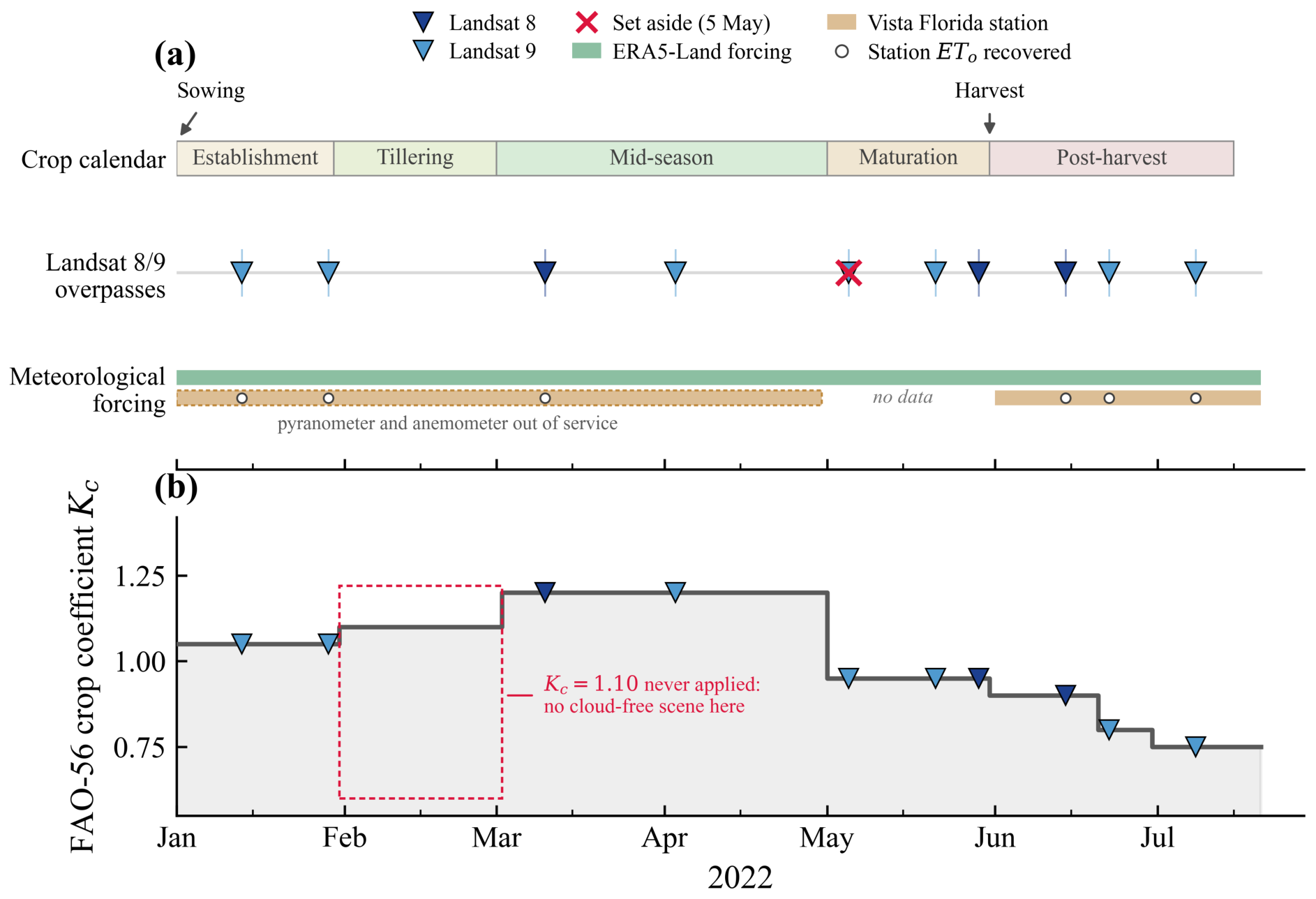
The hourly meteorological variables (temperature, humidity, wind, solar radiation, and pressure) were obtained from the ERA5-Land reanalysis [10] at the station location, and the elevation from the SRTM digital elevation model (30 m) [44]. ERA5-Land was chosen because the Vista Florida station lost its pyranometer and anemometer during January–April 2022 and has no record for May.
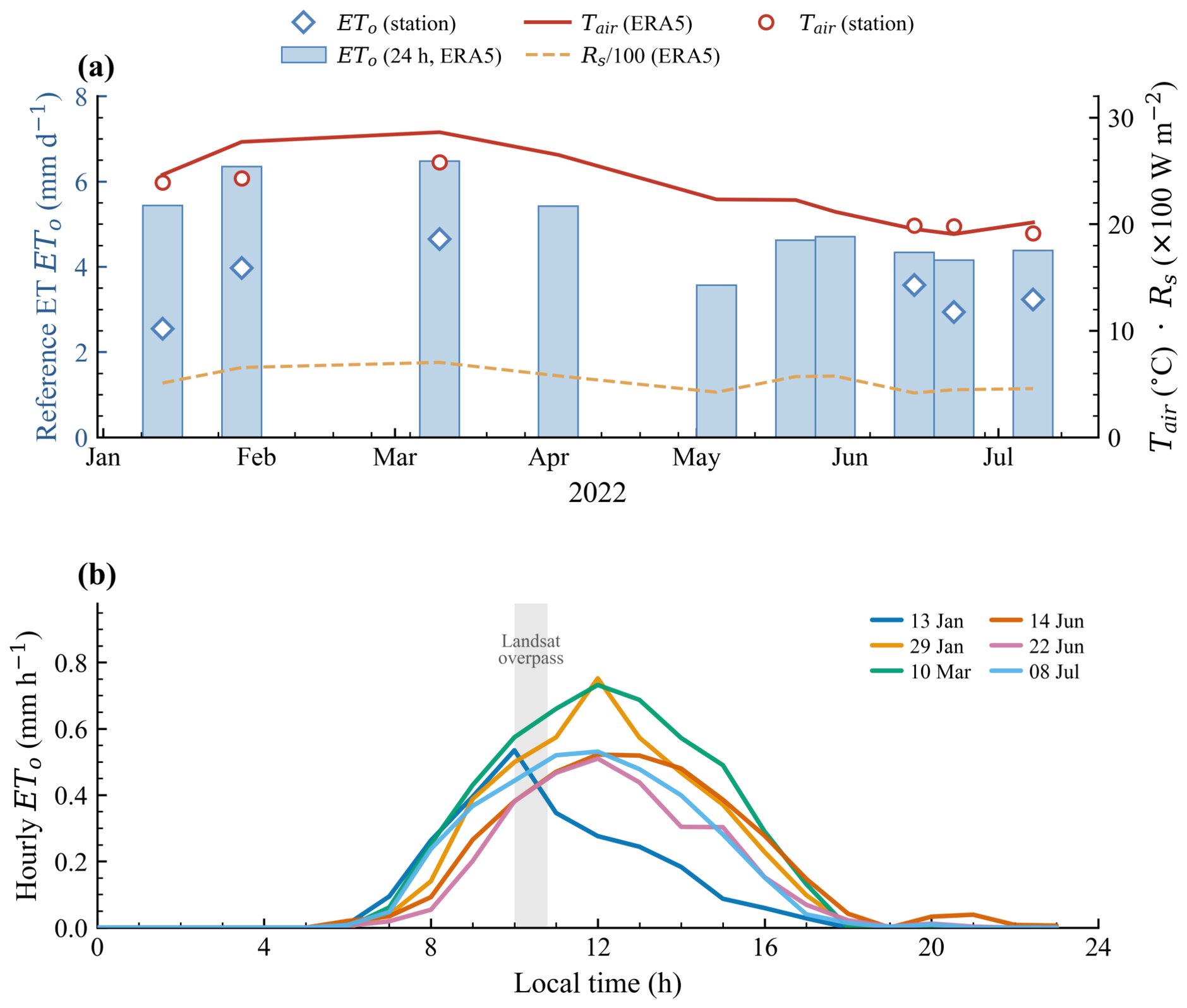
The available station data were cleaned and quality-controlled, and their ETo was computed with FAO-56; the procedure recovered six of the ten dates. The agreement between ERA5-Land and the quality-controlled station is examined in Figure S10 and Table S11, and a cross-check of the FAO-56 reference rebuilt from the station ETo is reported in Table S13. The meteorological conditions on the satellite overpass dates, which control evaporative demand, are summarised in Figure 2.
One consequence of this choice must be stated at the outset, because it conditions how the agreement statistics of Section 3.5 can be read. The same hourly ERA5-Land series supplies the reference ET that enters three separate places: the cold-pixel constraint of the METRIC internal calibration, the denominator of the reference-ET fraction used to extrapolate to daily values, and the K c E T o product that serves as the FAO-56 reference. The two quantities being compared are therefore not independent of each other, and any bias in the ERA5-Land reference propagates into both. The magnitude of that shared dependence, and the reason the comparison is nonetheless informative, are examined in Section 4.2; the station-based cross-check of Table S13 and the global-product cross-check of Section 2.5 were added to probe it from sources that do not share the reanalysis.

2.3. METRIC Model

METRIC [12] estimates daily ET from the latent heat flux obtained as the residual of the surface energy balance,
L E = R n G H ,
where R n is net radiation, G the soil heat flux, and H the sensible heat flux (all in W m−2).
Vegetation indices and surface temperature were computed from the image converted to top-of-atmosphere reflectance. The soil-adjusted vegetation index (SAVI) and the leaf area index (LAI) follow the formulation of Allen and Tasumi [12],
SAVI = ( 1 + L ) ( ρ NIR ρ R ) ρ NIR + ρ R + L , LAI = 1 0.91 ln 0.69 SAVI 0.59 ,
with L = 0.5 and ρ NIR , ρ R being the near-infrared and red reflectances. The broadband emissivity was estimated as ε 0 = 0.95 + 0.01 LAI (LAI ≤ 3; ε 0 = 0.98 for LAI > 3), and the surface temperature T s was obtained from band B10 converted to top-of-atmosphere spectral radiance and corrected for the narrowband emissivity. As noted in Section 2.2, that band carries a 100 m native observation distributed on the 30 m grid, so T s —and with it the sensible heat flux, the latent heat flux, and the ET derived from the energy balance—inherit the spatial support and the spatial correlation of the native thermal observations, whatever the grid on which they are mapped. Surface reflectance and albedo ( α ) were derived following Tasumi et al. [14].
Net radiation was solved as
R n = ( 1 α ) R s + ( R l R l ) ( 1 ε 0 ) R l ,
where R s is the incoming shortwave radiation and R l , R l the downwelling and upwelling longwave components. The soil heat flux was estimated as a function of LAI [12]:
G = 1.8 ( T s 273.15 ) + 0.084 R n , LAI < 0.5 , 0.05 + 0.18 e 0.521 LAI R n , LAI 0.5 .
The sensible heat flux is modelled as
H = ρ a c p d T r a h , d T = a T s + b ,
where ρ a is the air density, c p is the specific heat at constant pressure, r a h is the aerodynamic resistance to heat transport, and d T is the temperature difference between two heights near the surface. The coefficients a and b are calibrated internally by fixing H at two extreme anchor pixels [12]: at the cold pixel (full cover, well watered), L E cold = 1.05 λ E T o , inst is imposed (the factor 1.05 allows a full-cover, well-watered crop to slightly exceed the grass reference; λ , latent heat of vaporisation; E T o , inst , FAO-56 grass reference ET at overpass), so that d T cold = ( R n G L E cold ) r a h / ( ρ a c p ) ; at the hot pixel (dry bare soil), L E hot 0 is imposed, so that d T hot = ( R n G ) r a h / ( ρ a c p ) . From both, a = ( d T hot d T cold ) / ( T s , hot T s , cold ) and b = d T hot a T s , hot are obtained.

Automatic Anchor-Pixel Selection (CIMEC)

The reliability of the internal calibration rests entirely on the two anchor pixels, because the slope a and intercept b of d T = a T s + b are fixed from the ( T s , d T ) pair at the cold and hot extremes; a poorly chosen pair propagates directly into H and, as a residual, into L E . To remove operator subjectivity and make the run reproducible, anchor-pixel selection was automated with the CIMEC algorithm (Calibration using Inverse Modeling at Extreme Conditions) [33], which mimics the manual choice of a trained analyst while guaranteeing a consistent, documented rule across all ten dates.
The search was performed within a 5 km buffer around the ROI, large enough to contain both extremes and so secure the thermal contrast required for a stable calibration [12]. Candidate pixels were first screened to retain only physically meaningful agricultural surfaces, excluding open water (normalised difference vegetation index, NDVI 0.05 ), non-agricultural or anomalous cover (albedo outside [ 0.10 , 0.50 ] ), and steep terrain (slope > 5 ° ), where the one-dimensional energy balance and the d T T s relationship would not hold.
The cold pixel represents a fully vegetated, well-watered surface that transpires near the reference rate; it was sought among pixels with NDVI in the upper tail (NDVI ≥ 95th percentile) and a closed canopy (LAI 1.5 ), and the coldest of these was retained (lower 20th percentile of T s ). The hot pixel represents a dry, bare surface with negligible evaporation; it was sought among pixels with sparse vegetation (NDVI ≤ 10th percentile, LAI 0.5 ) and a bright, dry soil signature (albedo 0.13 ), retaining the hottest (upper 80th percentile of T s ). These joint vegetation–temperature–albedo criteria prevent the common failure modes of selecting a shaded or cloud-edge pixel as cold, or a water body or bright artificial surface as hot.
For robustness against single-pixel noise, about 20 candidates per class were sampled and the spatial median of the extreme thermal quartile was taken as the anchor value, and the physical consistency condition T s , cold < T s , hot was verified on every date. With the calibration fixed, the aerodynamic resistance r a h was solved iteratively, incorporating the Monin–Obukhov atmospheric stability correction (20 iterations) until d T and r a h converged. The selected anchor pixels are cached so that each run reproduces the same calibration.
The latent heat flux was obtained as the residual and converted to instantaneous ET via E T inst = 3600 L E / ( λ 10 6 ) , with λ = 2.45 MJ kg−1 the latent heat of vaporisation. Instantaneous ET was extrapolated to daily ET through the reference-ET fraction ( E T r F , relative to the FAO-56 grass reference ET E T o ) [12],
E T r F = E T inst E T o , inst , E T 24 h = E T r F · E T o , 24 h ,
where E T o , 24 h was integrated from 24 hourly ERA5-Land values, following the METRIC 24 h ET procedure [12] instead of a heuristic factor. The same grass reference ET E T o governs the cold-pixel constraint, the E T r F fraction, and the K c E T o reference (Section 2.5); the ET retrieval and its evaluation thus share a single reference, which makes them directly comparable but also mutually dependent, a point developed in Section 4.2.

2.4. Implementation on Google Earth Engine

The model was implemented in Python 3.10 (Python Software Foundation, Wilmington, DE, USA), using the Earth Engine Python API v1.7.22, geemap v0.37.2, NumPy v2.2.6, pandas v2.3.3, GeoPandas v1.1.3 and rasterio v1.4.4, with the workload split between the Google Earth Engine servers and the local session [27]. Everything that operates on full scenes runs server-side: the archive query by path/row and date, the per-pixel cloud screening on QA_PIXEL, the conversion to top-of-atmosphere reflectance and radiance, the albedo, the vegetation indices and leaf area index, the surface temperature, and the percentile reductions over the 5 km buffer from which the anchor candidates are drawn. What returns to the local session is small: the anchor-pixel properties, the per-date calibration scalars, and the exported ET rasters. The Monin–Obukhov stability loop and the solution of d T = a T s + b are solved locally, being sequential by nature and operating on a handful of numbers per date rather than on imagery.
Three properties of the platform decided its use. The Landsat archive, ERA5-Land, and SRTM are co-located in a single catalogue, so the three inputs are queried in one place instead of being downloaded from three providers and reprojected onto a common grid. Nothing is downloaded before the final product, which makes the same script reproducible on any machine with an account. And the computation scales to the whole valley without changing the code, the condition for moving from the 113 ha block to operational coverage [26,45].
Each alternative has a limitation for this application. A desktop workflow gives full control but ties reproducibility to one machine’s software stack and does not scale. EEFlux [30] is the closest tool, being METRIC on Landsat served from the same platform, but its calibration is applied internally and the user cannot inspect or replace the anchor-pixel selection, which is precisely the step this study set out to automate. geeSEBAL [28] and SEBALIGEE [29] are open and modifiable, yet they implement SEBAL, whose calibration is anchored to a temperature difference rather than to a reference-ET constraint at the cold pixel. SSEBop is operational and well validated, but its ready-made products cover the conterminous United States rather than South America [31]. Federated open interfaces such as openEO would remove the dependence on a single provider and are the route by which this workflow could be made portable [46]. Google Earth Engine was retained as the only option combining co-located forcing, a free research tier, and full control over the anchor-pixel rule. This is a design justification rather than a measured comparison, since no peer-reviewed benchmark of these platforms against one another is available.

2.5. Benchmarking Against the FAO-56 Reference and Spatial Analysis

E T METRIC was compared with the FAO-56 reference ET, E T F A O - 56 = K c · E T o , 24 h . The word comparison is used deliberately in place of validation. FAO-56 is itself a model, which estimates crop ET from a reference ET and a tabulated coefficient under standard conditions, and it therefore provides no independent measurement of actual ET; the agreement statistics below quantify the consistency between two modelling approaches, not the absolute accuracy of either. The absence of independence is compounded by the shared forcing described in Section 2.2, since the same ERA5-Land E T o constrains the cold pixel, sets the reference-ET fraction and forms the FAO-56 product. A validation in the strict sense would require direct measurements of actual ET from eddy covariance, a weighing lysimeter or a soil water balance, none of which is available at this site; establishing them is identified as the first priority for future work in Section 4.6. The reference itself carries uncertainty: a meta-analysis of crop coefficients in arid and semi-arid regions shows that the tabulated values require local calibration [47], and a single coefficient cannot separate the evaporation of the water layer from canopy transpiration, which a dual coefficient formulation for water-saving paddy fields does explicitly [48]. The crop coefficient K c comes from the FAO-56 curve for flooded rice and is assigned by phenological stage according to the days elapsed since sowing: 1.05 (initial), 1.10 (development), and 1.20 (mid-season), with decreasing values (from 0.95 to 0.75) towards senescence and post-harvest, kept high by the persistent water layer. The values applied on each date are listed in Section 3.5. None of the ten cloud-free scenes coincided with the development stage, so the 1.10 value was not actually applied. Performance was quantified by comparing the ET estimated by METRIC ( P i = E T METRIC , i ) against the FAO-56 reference ( O i = E T F A O - 56 , i ) over the n valid dates, with means P ¯ and O ¯ .
The reported metrics are the root mean square error (RMSE), the mean absolute error (MAE), the mean bias error (MBE), the percent bias (PBIAS), and the coefficient of determination ( r 2 , squared Pearson correlation):
RMSE = 1 n i = 1 n P i O i 2
MAE = 1 n i = 1 n P i O i
MBE = 1 n i = 1 n P i O i
PBIAS = 100 i = 1 n P i O i i = 1 n O i
r 2 = i = 1 n O i O ¯ P i P ¯ i = 1 n O i O ¯ 2 i = 1 n P i P ¯ 2 2
A positive MBE (in mm d−1) and a positive PBIAS (the same bias normalised by the total observed ET, in %) both indicate that METRIC overestimates the FAO-56 reference; PBIAS expresses the overall over- or underestimation as a percentage of the reference water use [49].

2.5.1. Quality Control of the Individual Dates

The internal calibration is not equally well conditioned on every scene, so scene-level quality control was defined before the error statistics were computed. Its criteria are stated here as reproducible thresholds, and their provenance is declared: they were not pre-registered. The calibration diagnostics of the ten dates were inspected first; one date stood out on several of them at once, and the criteria were then formalised so that any exclusion could be reproduced by a third party rather than rest on the authors’ judgement. Once formalised, they were applied uniformly to all ten dates. A scene is set aside from the summary statistics if it fails any of the following:
(i)
Thermal contrast. The cold–hot difference Δ T s 8 K. Below that, the two anchors span too narrow a range for the regression d T = a T s + b to be well conditioned, and small errors in either extreme swing the slope.
(ii)
Cold-anchor vegetation. The NDVI of the selected cold pixel 0.50 . The cold anchor is meant to represent a fully vegetated surface transpiring near the reference rate; below that value, it no longer does.
(iii)
Consistency of the reference forcing. The daily E T o within ± 20 % of the value linearly interpolated from the two temporally adjacent scenes. Evaporative demand on this coast varies smoothly through the season, so a larger departure indicates a problem in the forcing rather than a meteorological event.
The three criteria were applied to all ten scenes before any error statistic was computed; the outcome and the diagnostic values behind it are reported in Section 3.5. Whatever the outcome, the summary statistics are given both with and without any scene set aside, so that the effect of the decision on the reported error remains visible.

2.5.2. Cross-Check Against Independent Global ET Products

Because the FAO-56 comparison shares its reference E T o with the METRIC calibration, two global ET products were added that share neither that forcing nor the energy balance formulation. MOD16A2GF (collection MODIS/061) applies a Penman–Monteith formulation driven by the MODIS land cover and leaf area index together with reanalysis meteorology from the Global Modeling and Assimilation Office, and delivers 8-day totals at 500 m. PML-V2 couples a Penman–Monteith–Leuning evaporation model to a carbon assimilation model and delivers 8-day daily means, also at 500 m. Both were extracted over the ROI on Google Earth Engine and each Landsat date was matched to the 8-day composite containing it. The limitation of the exercise is stated up front: only 11 pixels of 500 m cover the 113 ha block, so the products describe the field together with the surrounding desert, roads, and neighbouring plots, and they can corroborate the shape of the seasonal trajectory but not the absolute magnitude of ET over the crop. This behaviour is documented: global ET products evaluated against ground measurements over irrigated agriculture in arid environments depart appreciably from the field values [50], and a formal error attribution traces the departure to coarse resolution, meteorological forcing, and parameterisation [51]. Agreement is reported over the nine quality-controlled dates and, separately, over the seven dates from 1 March onwards, once the canopy is established and the free water layer no longer dominates the surface. The results are given in Section 3.5 and detailed in Figure S13 and Table S14.

2.5.3. Spatial Analysis

The per-parcel mean ET was cross-referenced with the sowing method and cultivar attributes of the 189 parcels to analyse the spatial variability between and within the management groups. Differences in season-mean ET between sowing methods and among cultivars were tested with the non-parametric Mann–Whitney and Kruskal–Wallis tests, respectively ( α = 0.05 ).
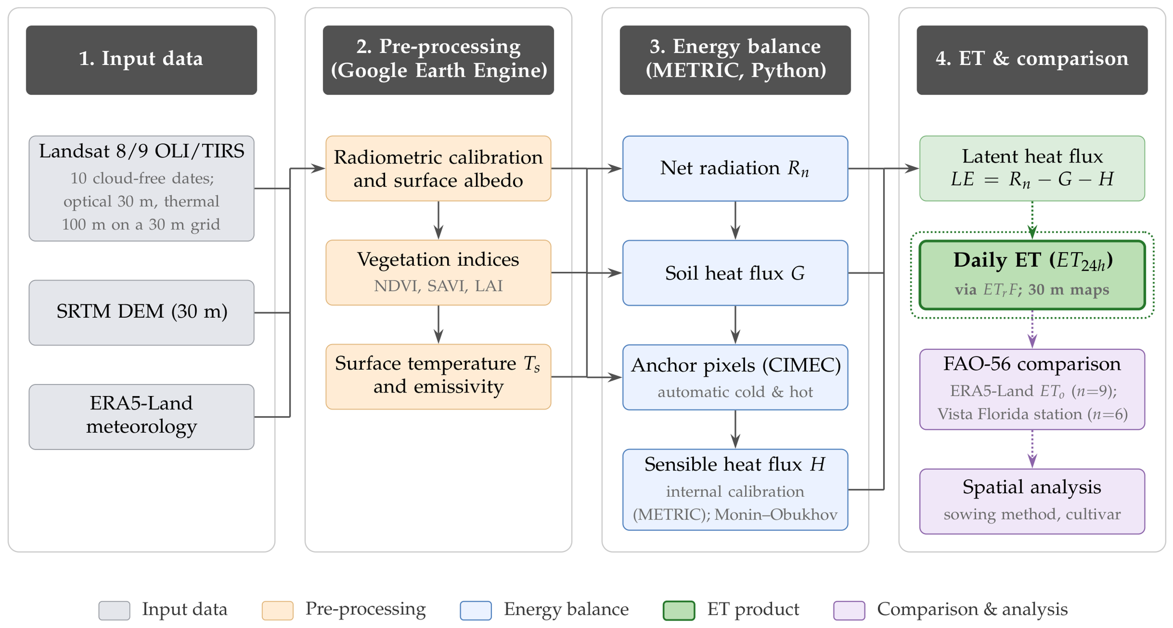
The complete procedure, from the cloud inputs to the ET products and their evaluation, is organised into a reproducible four-stage workflow summarised in Figure 3. Each block of that diagram is described below in the order in which it is executed.
The first stage assembles the input data. The Landsat 8/9 OLI/TIRS block supplies the ten cloud-free scenes, the SRTM block the 30 m elevation that sets the atmospheric pressure and the terrain slope used to reject steep anchor candidates, and the ERA5-Land block the hourly meteorology from which the instantaneous and 24 h reference ET are computed. The three converge on the pre-processing chain rather than feeding it in sequence, because each is required by more than one downstream block.
The second stage pre-processes the imagery in Google Earth Engine. Its three blocks run in order on every scene: radiometric calibration converts the raw digital numbers to top-of-atmosphere reflectance and radiance and derives the albedo α ; the vegetation index block computes NDVI, SAVI, and, from SAVI, the leaf area index; and the surface temperature block obtains the broadband emissivity from LAI and uses it to correct the thermal radiance into T s . The order is not interchangeable, since the emissivity correction requires the LAI computed in the preceding block.
The third stage solves the surface energy balance in Python. Net radiation combines the incoming shortwave weighted by albedo with the longwave balance; the soil heat flux follows from R n and LAI through Equation (4); the anchor-pixel block applies the CIMEC rule within the 5 km buffer to select one cold and one hot pixel automatically, which is the step that replaces operator judgement; and the sensible-heat-flux block closes the internal calibration, the two anchors fixing the coefficients of d T = a T s + b while the aerodynamic resistance is solved iteratively with the Monin–Obukhov correction. R n , G and H leave the stage together because the residual in the next stage needs all three.
The fourth stage derives the ET product and evaluates it. The latent heat flux is obtained as the residual L E = R n G H , converted to an instantaneous ET and extrapolated to the daily value through the reference-ET fraction, which yields the 30 m maps of E T 24 h . Evaluation then follows two lines, drawn as dotted arrows to mark that they assess rather than produce: the comparison against the FAO-56 reference and the spatial analysis of the per-parcel means by sowing method and cultivar.
The temporal deployment of the campaign, from sowing to harvest with the ten Landsat acquisitions and the availability of each meteorological source, is summarised in Figure 4.

3. Results

3.1. Surface Variables

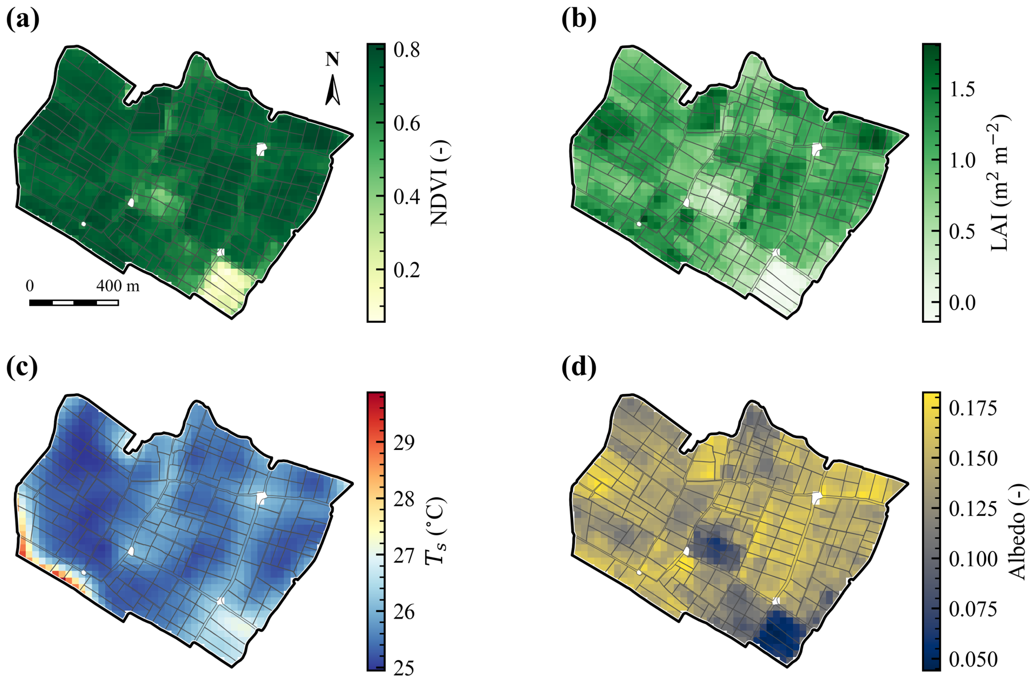
The field-mean NDVI followed crop phenology, peaking at 0.69 on 10 March, with a maximum LAI of 1.04 on 3 April, and declining towards harvest; the surface temperature, 25.8 °C at full cover (10 March), rose towards the dry season to 32.5 °C in July (Table 2). Figure 5 shows the spatial distribution of the four surface variables (NDVI, LAI, T s , and albedo) for 10 March, a representative mid-season date corresponding to the peak of canopy cover. On that date, the canopy covers the field fairly homogeneously, with high NDVI and LAI and little contrast between parcels; the lowest surface temperatures occur over the parcels with the densest canopy and standing water, and albedo remains low under full vegetation cover, so the largest intra-field contrasts concentrate at the edges and in the parcels established later. The multi-date spatial evolution of the four variables over the ROI is shown in Figures S2–S5 of the Supplementary Materials, and their per-date intra-field distribution, for LAI and albedo, is shown in Tables S3 and S4.

3.2. Internal Calibration and Anchor-Pixel Selection

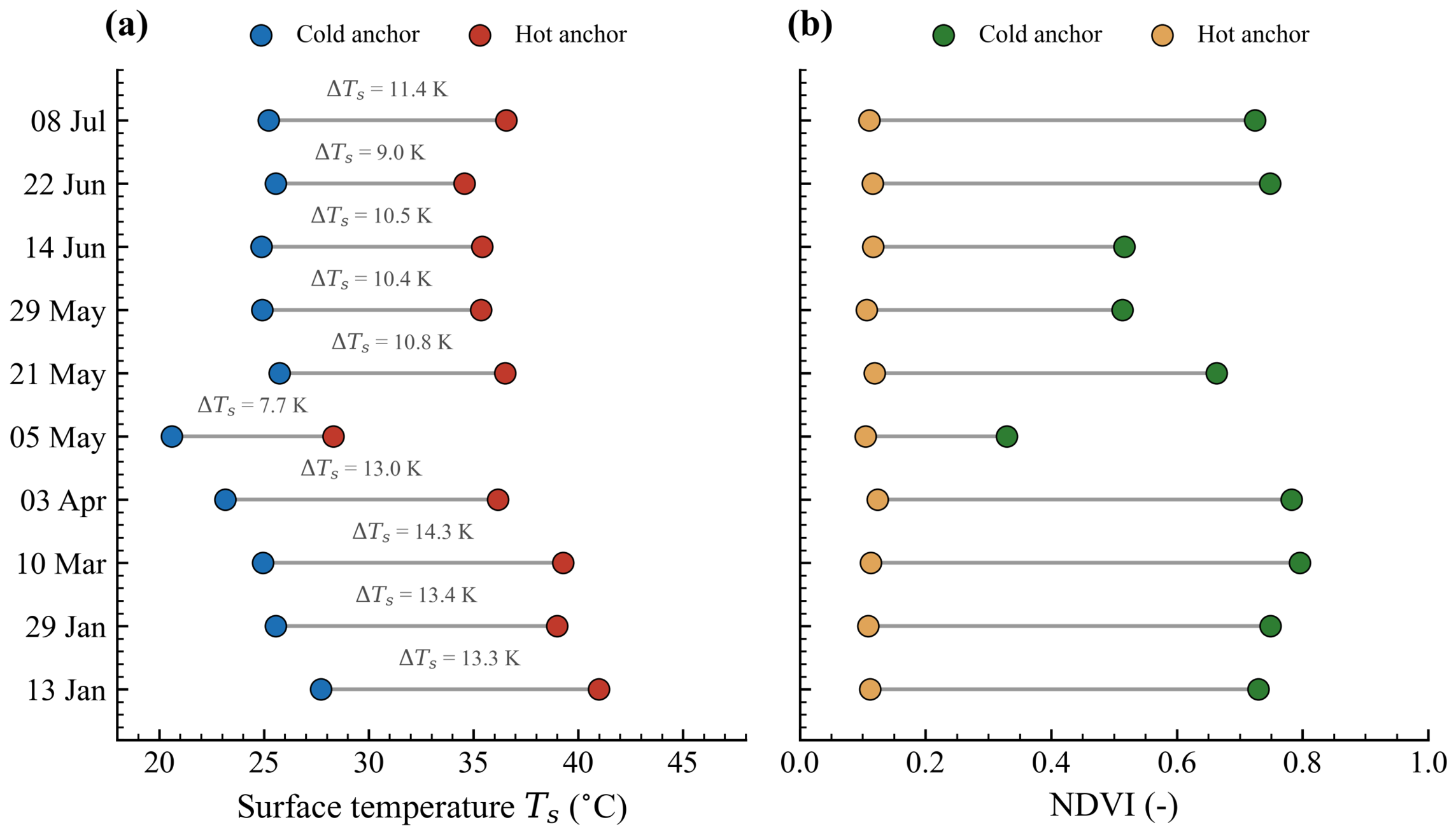
The automatically selected anchor pixels showed a thermal contrast Δ T s of 7.7 to 14.3 K, within the range recommended by Allen et al. [12], with a clear NDVI separation between the cold pixel (dense vegetation) and the hot one (bare soil) that supports a robust calibration of the sensible heat flux in each scene (Figure 6); their full properties (NDVI, SAVI, LAI, albedo, R n , and G) are detailed in Table S1 of the Supplementary Materials. From these anchor pixels, the coefficients of the calibration function d T = a T s + b (Table 3) were solved for each date: the slope a ranged from 0.08 to 0.36 and the intercept b from 21 to 102 , and the Monin–Obukhov stability iteration converged in 20 steps on all dates (Figure S12). The steepest slope ( a = 0.36 ; 5 May) corresponds to the lowest thermal contrast ( Δ T s = 7.7 K): in mid-autumn, the coldest, most-vegetated candidate available within the 5 km search buffer was less vigorous than at peak season (cold-pixel NDVI 0.33; full anchor properties in Table S1), which narrows the range over which d T is fitted and makes 5 May the weakest calibration of the series; this date is consequently set aside by the quality control of Section 2.5.1, and the effect of that decision on the reported error is shown in Section 3.5.

3.3. Energy Balance Components

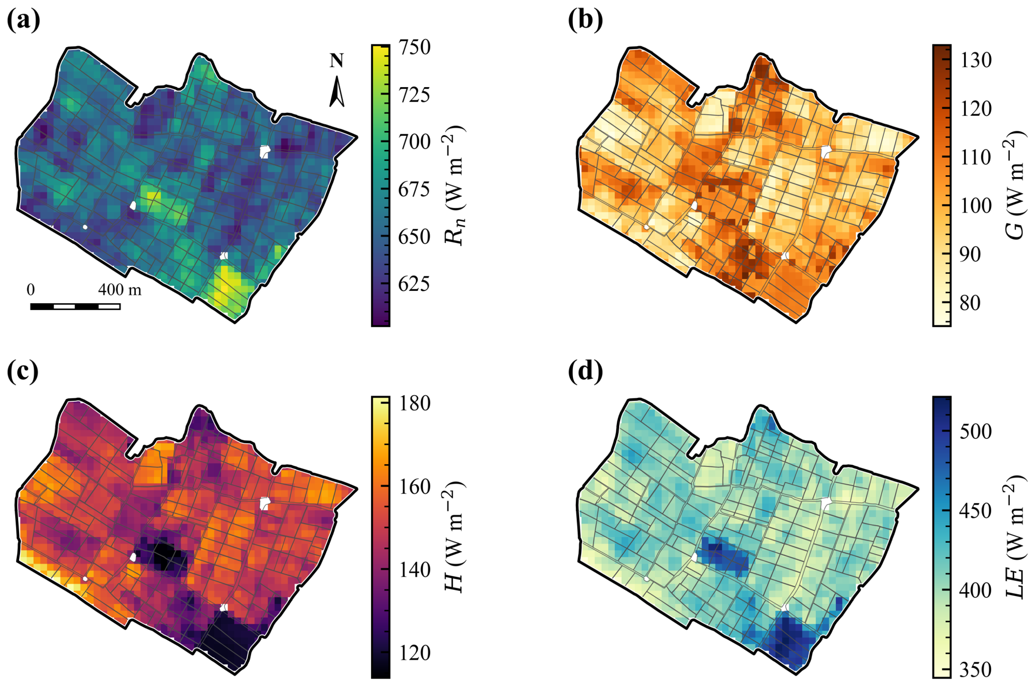
The mean net radiation showed a decreasing trend over the season, from ∼677 W m−2 in summer to ∼489 W m−2 towards the austral winter (Table 4), in line with the seasonal decline in incoming solar radiation and the rise in albedo (0.11 to 0.19; Table 2) as the canopy senesced. The latent heat flux ( L E ) was highest during flooding and establishment and lowest after harvest, inversely to the sensible heat flux (Figure 7). Spatially, on 10 March, the highest L E coincides with the dense-canopy, well-flooded parcels, whereas H rises at the edges and in the lower-cover parcels, where the more exposed soil warms the air; net radiation and the soil heat flux, by contrast, show a more uniform pattern across the field. The multi-date spatial evolution of the four energy balance components and their per-date intra-field distribution are documented in Figures S6–S9 and Tables S5–S8 of the Supplementary Materials.

3.4. METRIC-Derived Daily Evapotranspiration and Its Seasonal Dynamics

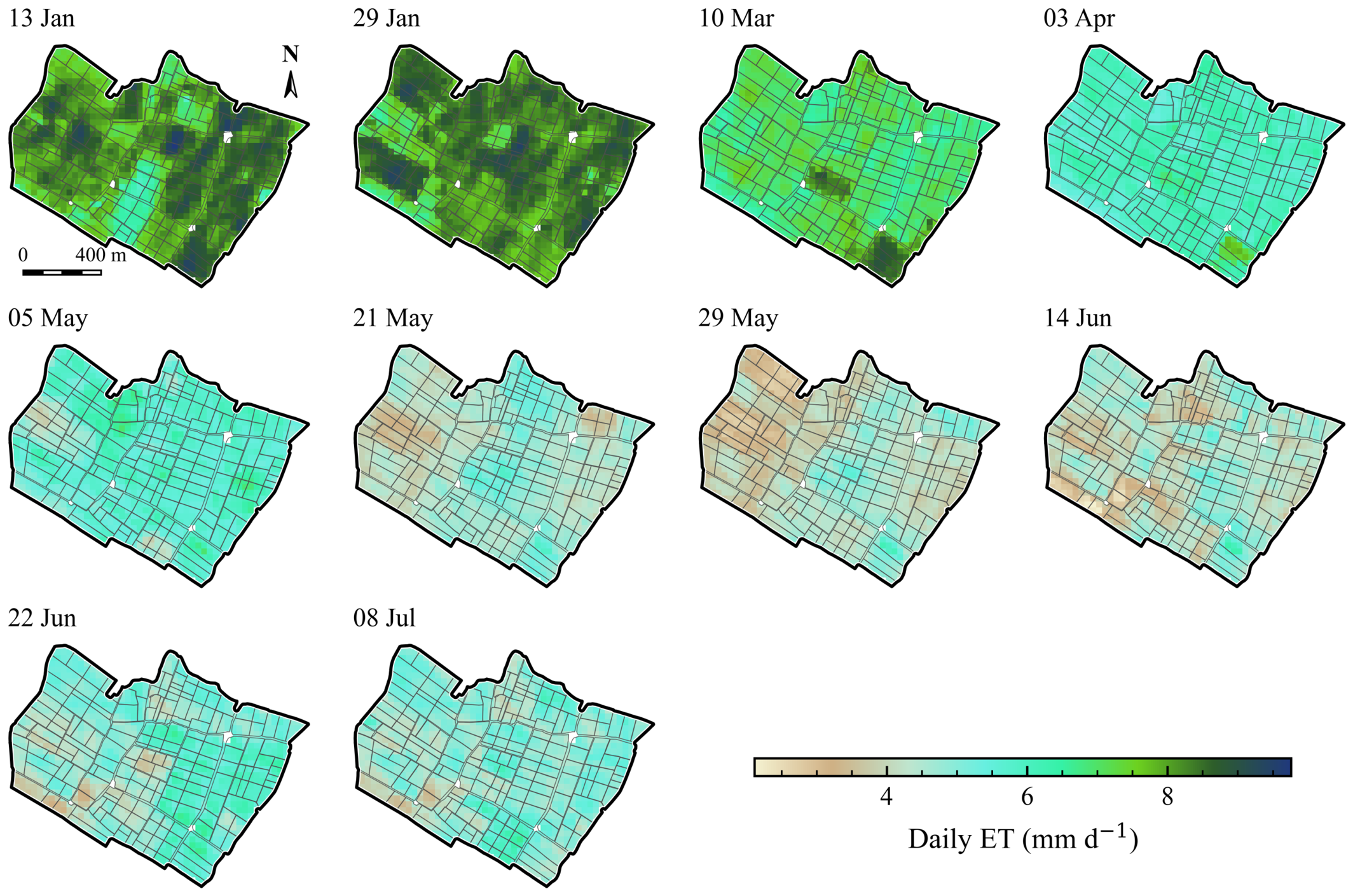
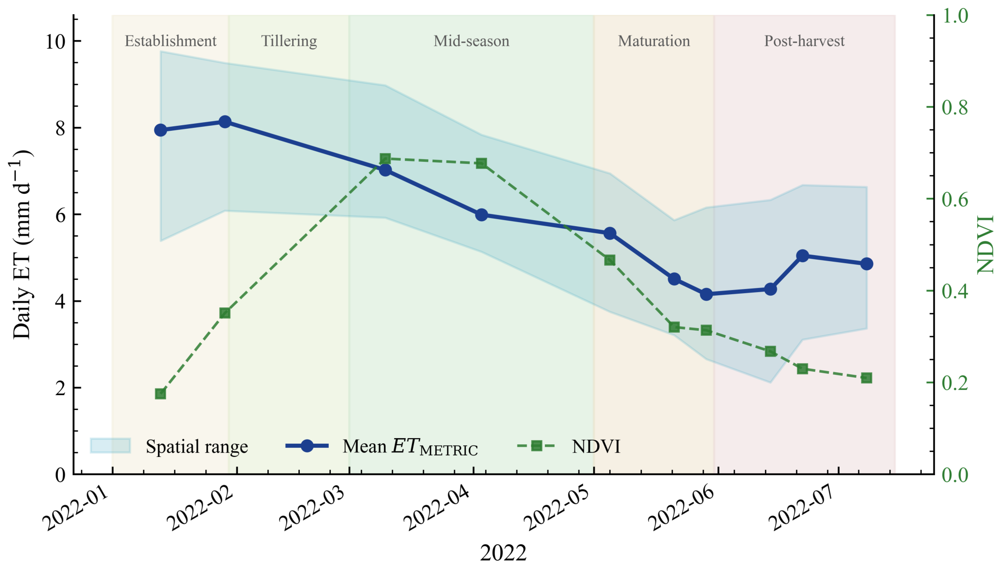
The daily field-mean ET ranged from 4.2 to 8.1 mm d−1 (Table 5). The highest values occurred during flooding and establishment (7.9–8.1 mm d−1 in late January), when the evaporation of the free water layer dominates water use even at low NDVI (0.18–0.35); from full cover onwards, ET declined towards harvest, down to about 4.2 mm d−1 by late May, with a slight rebound on the post-harvest dates when the field retained standing water. The temporal dynamics of the mean ET, together with NDVI, are summarised in Figure 8.
The ET maps for the ten dates (Figure 9) reveal this seasonal decline and a substantial intra-field spatial variability on all dates (coefficient of variation of 6 to 14%; Figure S11 and Table S2), reflecting the heterogeneity of water management and sowing dates.

3.5. Comparison with the FAO-56 Reference and with Independent ET Products

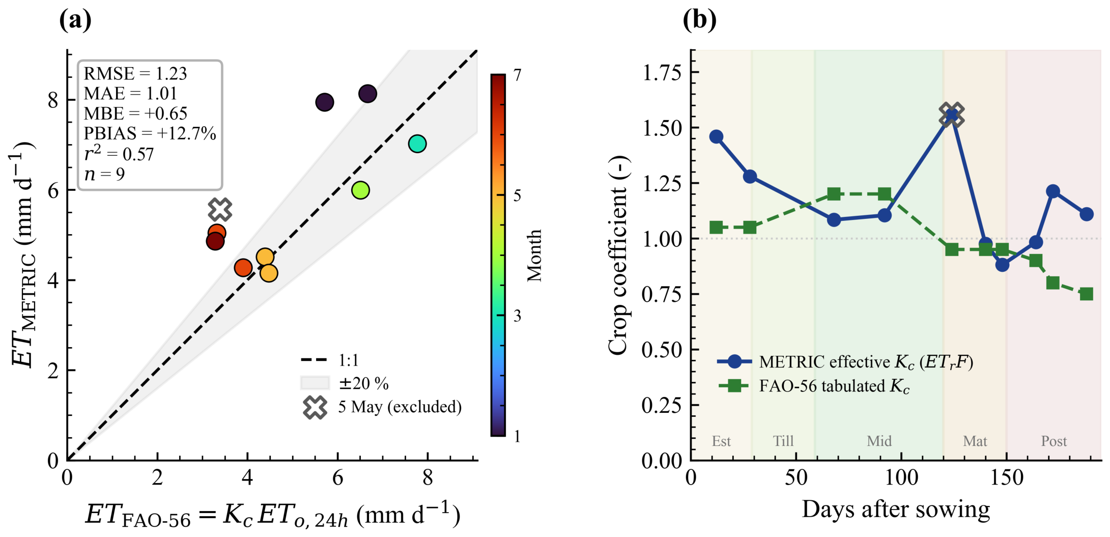
The integrated reference ET decreased from ∼6.5 mm d−1 in midsummer (March) to 3.6–4.7 mm d−1 in the austral autumn–winter (May–July), in line with the reduction in solar radiation and air temperature as the season progressed (Table 6). The 5 May date was excluded from the summary statistics by the quality control described in Section 2.5.1. Applied to the ten scenes, the three criteria flag exactly one, and that scene fails all three at once: its ERA5-Land reference ETo was anomalously low (∼3.6 mm d−1, 27% below the value interpolated from the adjacent scenes and even below later dates such as 21 and 29 May), it had the lowest thermal contrast of the season ( Δ T s = 7.7 K against 9.0 to 14.3 K on the other nine dates; Table 3), and its cold anchor reached an NDVI of only 0.33, well below the 0.51 to 0.80 spanned by the remaining dates and the only value beneath the 0.50 threshold, with an albedo of 0.39 against 0.16 to 0.25 elsewhere, which is not the signature of a well-watered canopy (Table S1). No other scene fails any criterion, although two late-season dates approach the vegetation threshold (NDVI 0.51 on 29 May and 0.52 on 14 June) and one approaches the thermal one (22 June, Δ T s = 9.0 K); on each of the three diagnostics, 5 May is nonetheless separated from the next most marginal date by a clear gap. No station data were available to verify it. The scene is retained for the ET mapping and seasonal description, but its FAO-56 discrepancy ( + 64 % ) is unreliable and would dominate the error statistics.
Over the nine remaining dates, METRIC showed a mean positive bias against E T F A O - 56 of + 0.65 mm d−1 (RMSE = 1.23 , MAE = 1.01 mm d−1; PBIAS = + 12.7 % ; r 2 = 0.57 ; n = 9 ; Table 6), i.e., an overestimation of the seasonal FAO-56 water use of about 13% (including 5 May, the bias rises to + 0.80 mm d−1, RMSE = 1.35 , PBIAS = + 16.2 % , r 2 = 0.53 ). Because the same grass reference E T o underlies the cold-pixel constraint, the E T r F fraction and the K c E T o reference, these figures quantify the consistency between two modelling approaches and not the accuracy of either: the comparison is an agronomic benchmark rather than an independent validation of the absolute ET magnitude. The overestimation concentrated during flooding (January, + 22 to + 39 % ) and on post-harvest dates ( + 48 to + 52 % in late June and July), when the tabulated K c declines while flooded rice maintains high evaporation; at full cover (March–April), the two estimates converged (differences of 8 to 10 % ), as seen in the 1:1 scatter of Figure 10a. This dynamic is summarised by the effective crop coefficient retrieved by METRIC ( E T r F = E T METRIC / E T o , 24 h ), which exceeded the tabulated FAO-56 K c during flooding (1.3–1.5 vs. 1.05) and after harvest (around 1.0–1.2 vs. 0.75–0.90), and converged with it at full cover (Figure 10b).
As a check on the source of the ETo, the FAO-56 reference ( K c E T o ) was reconstructed using the ETo measured at the quality-controlled station on the six operational dates (Table S13). The positive bias of METRIC against the reference persisted and was even larger with the station ETo (MBE = + 2.81 mm d−1; n = 6 ), which indicates that the tabulated crop coefficient underestimates the actual ET of flooded rice regardless of the meteorological source. This difference should be read as an upper bound: the station ETo is somewhat lower than the ERA5-Land one (Figure S10) and, in January–March, the inoperative anemometer ( u 2 0 ) reduces the aerodynamic term and further depresses the reference ETo.
Neither of those two references escape the ERA5-Land dependence entirely, so the retrieval was also set against two global ET products whose formulation and meteorological forcing are independent of both METRIC and the reanalysis (Section 2.5.2; Figure S13 and Table S14). Over all nine quality-controlled dates, the correlation with E T METRIC is weak ( r = + 0.24 for MOD16A2GF and + 0.29 for PML-V2), but the disagreement is not spread through the season: it is concentrated in January. Restricted to the seven dates from 1 March onwards, once the canopy is established, the correlation rises to + 0.63 and + 0.91 , respectively, and both products reproduce the decline towards harvest that METRIC retrieves. The pattern is what the physics predicts. MOD16A2GF and PML-V2 are both driven by canopy variables, so during flooding and establishment, when a free water layer evaporates at 7.9 to 8.1 mm d−1 under an NDVI of 0.18 to 0.35, they see almost nothing: PML-V2 returns 0.58 and 1.10 mm d−1 on those two dates. The FAO-56 reference, which is also canopy-driven through K c , correlates more closely with the products than METRIC does ( r = + 0.69 and + 0.77 over all dates), which places METRIC on one side of the divide and the three canopy-driven estimates on the other, precisely over the stages where the crop coefficient was already found to fall short. In absolute terms, both products stay far below the field values, by a factor of about 2.5 for MOD16A2GF, an offset expected from the 11 pixels of 500 m that cover the block and dilute an irrigated field into the surrounding desert; the exercise therefore corroborates the seasonal trajectory and the physical interpretation of the bias, not the magnitude of ET.

3.6. Variability by Sowing Method and Cultivar

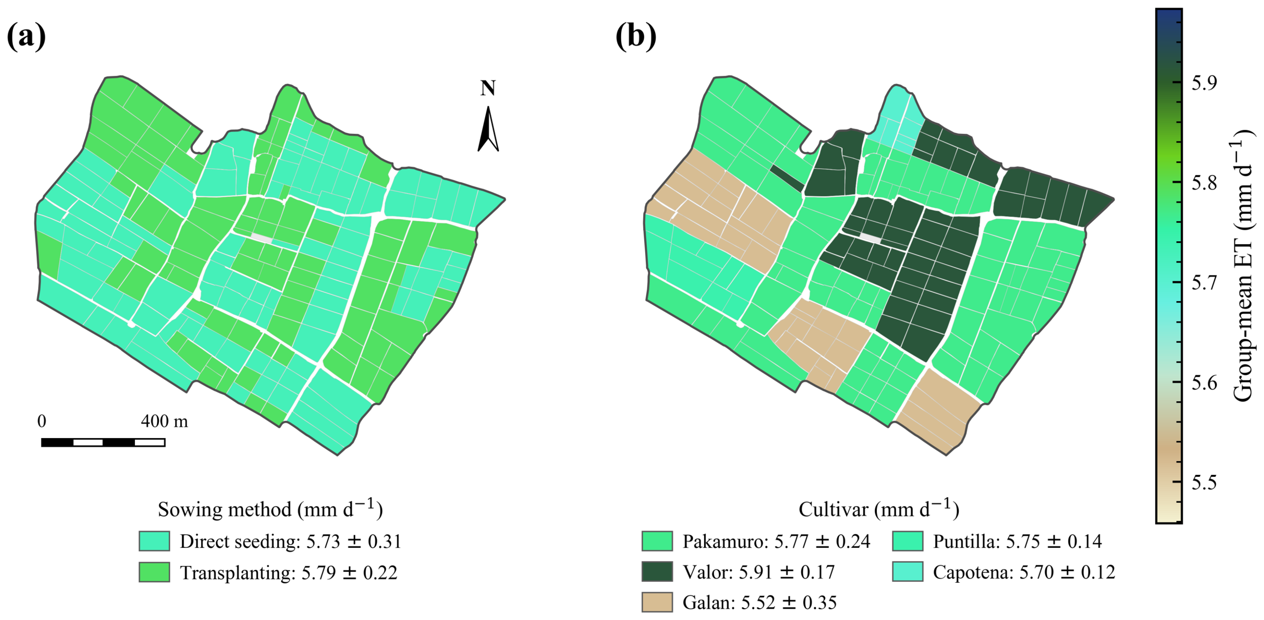
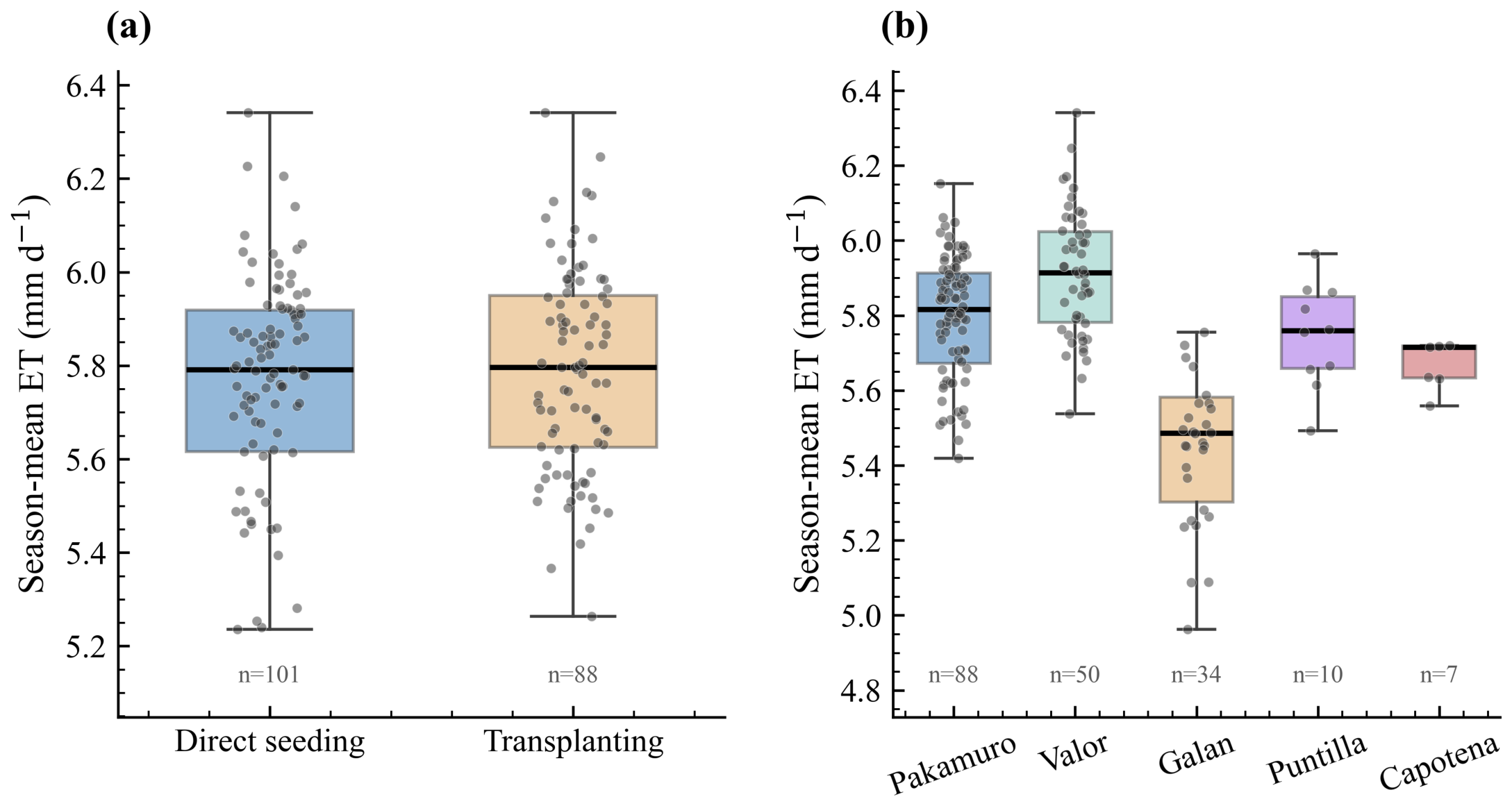
The season-mean ET did not differ significantly between sowing methods (direct seeding 5.73 vs. transplanting 5.81 mm d−1; Mann–Whitney test, p = 0.42 ). Among cultivars, the differences were statistically significant (Kruskal–Wallis, p < 0.001 ) but small in magnitude: the means ranged from 5.61 to 5.93 mm d−1, a range of 0.32 mm d−1 equivalent to ∼6% of the mean (Table 7). As Figure 11 shows, the per-group ET distributions overlap widely, and the season-mean ET projected onto the parcels by management group (Figure 12) confirms how small these differences are. Both the contrast between sowing methods and that among cultivars is far smaller than the intra-field spatial variability (CV of 6 to 14%, Figure S11), indicating that, in this system, the heterogeneity of water use responds more to water management and local phenology than to sowing method or cultivar. The per-cultivar and per-sowing-method ET detail for each date is reported in Tables S9 and S10 of the Supplementary Materials.

4. Discussion

4.1. Seasonal ET Dynamics and Energy Balance

The seasonal pattern of ET is physically consistent with the phenology of flooded rice and with the dynamics of the energy balance components. The maximum values, around 8 mm d−1 during flooding and establishment, coincide with the highest net radiation and the dominance of the latent heat flux, and decline steadily as the seasonal drop in solar radiation lowers R n and canopy senescence raises albedo, a seasonal trajectory of paddy ET driven by radiation and crop development that is also reported by remote-sensing studies of flooded rice [52]. The direct evaporation of the free water layer, together with the incipient transpiration of the canopy, explains why ET remains high in these early stages despite a still-low vegetation index. This range agrees with direct lysimeter measurements in flooded paddies, which record a daily ET of up to ∼8 mm d−1 and crop coefficients above the tabulated FAO-56 values [21]. The estimation of paddy ET with field-scale energy balance models, including dual-source approaches [53], further supports the suitability of this framework for flooded systems.

4.2. Comparison with FAO-56 and Interpretation of the Bias

The positive bias against FAO-56 ( + 0.65 mm d−1) is consistent with METRIC recovering processes that the crop-coefficient approach does not represent: the evaporation of the free water layer during flooding and the residual evaporation of moist soil and stubble after harvest, stages in which the tabulated K c underestimates actual water use. The concentration of the overestimation in those two stages, together with the convergence at full cover ( 8 to 10 % ) when canopy transpiration governs water use, supports this interpretation: the pattern suggests that the model captures the transition from a surface dominated by free water to one dominated by vegetation. The attribution is nevertheless indirect. No direct measurement of actual ET (eddy covariance or lysimeter) is available at this site, so uncertainties associated with the METRIC formulation, the anchor-pixel calibration, the meteorological forcing, and the parameterisation cannot be fully excluded, and the divergence should be read as consistent with these surface processes rather than as demonstrating that it is unrelated to model or retrieval errors. This overestimation is consistent with what has been reported for energy balance models in arid zones, which overestimate ET over dry, stubble-covered surfaces relative to field measurements [19], and with the comparison of METRIC against FAO-56 in paddies [18]. That the bias persists, and even increases, when the reference is reconstructed with the ETo measured at the quality-controlled station (MBE = + 2.81 mm d−1; Table S13) suggests that it is not attributable to the meteorological source alone. Part of the gap is also a property of the reference rather than of the retrieval: a single tabulated coefficient lumps the evaporation of the water layer with canopy transpiration, which is exactly the separation a dual coefficient formulation makes in water-saving paddies [48], and tabulated coefficients in arid climates carry substantial variability of their own [47]. In flooded systems, therefore, the standard FAO-56 K c should be used with caution as the sole reference for water use.
The shared reliance on ERA5-Land deserves to be examined rather than merely listed, because it determines what the agreement statistics can and cannot establish. One hourly reanalysis series supplies the reference ET in three places at once: the cold-pixel constraint L E cold = 1.05 λ E T o , inst , the denominator of the reference-ET fraction, and the K c E T o product. The consequence is asymmetric, and the asymmetry is what makes the comparison still worth making. A multiplicative bias in E T o largely cancels in the quantity actually compared, because METRIC returns E T 24 h = E T r F · E T o , 24 h while the reference is K c · E T o , 24 h , so the ratio reduces to E T r F / K c , in which the reanalysis value divides out. The stage-dependent pattern of Section 3.5 is therefore robust to the level of the forcing and reflects the crop coefficient rather than the meteorology. What does not survive is the absolute magnitude: an E T o biased high would inflate E T METRIC and E T F A O - 56 together, leaving their agreement untouched while both depart from the true ET, and neither this comparison nor the station cross-check can rule that out. That is why the two global products of Section 2.5.2 were added: independent of both the reanalysis and the energy balance, they corroborate the seasonal trajectory while confirming, through their own coarse-pixel bias, that the absolute magnitude remains beyond the reach of any of these references. Establishing it requires direct flux or lysimeter measurement.

4.3. Sensitivity to Anchor-Pixel Selection and Reproducibility

Automating anchor-pixel selection (CIMEC) removes operator subjectivity and shortens processing, improving reproducibility relative to manual selection [33,54]. METRIC-derived ET is nonetheless sensitive to the choice of the thermal extremes: global sensitivity analyses identify the selection of the cold and hot pixels, together with solar radiation, as the factors that most condition the uncertainty [55], while the area size and the availability of representative extremes affect the calibration [34,56]. The search within a 5 km buffer around the ROI secured the required thermal contrast on most dates ( Δ T s of 7.7 to 14.3 K); the single low-contrast, weakly-vegetated case (5 May) was identified and set aside from the quantitative comparison, which underlines the importance of a consistent, documented extreme-selection strategy and of screening marginal scenes.

4.4. Spatial Variability and Irrigation Management

Unlike FAO-56, the METRIC–Google Earth Engine workflow resolves the spatial variability of ET at 30 m operationally, without downloading or locally pre-processing imagery. Although the means between sowing methods and among cultivars were similar, in contrast to studies where METRIC does discriminate water use between irrigation systems [57], the intra-field variability detected (CV of 6 to 14%) is information directly useful for field-scale irrigation scheduling, as has been shown when mapping ET for precision irrigation in other crops [9]. This capability is especially relevant in rice systems moving from continuous flood irrigation towards water-saving strategies such as alternate wetting and drying (AWD), whose water-productivity advantages are well documented [58,59] and which are already being tested on the northern coast of Peru [36]. Field-scale ET maps provide the spatial basis to target and monitor this type of management.

4.5. Limitations

The main limitation is the absence of in situ ET measurements (lysimeter or eddy covariance), which prevents a direct validation of the absolute magnitude; the comparison relied on the FAO-56 agronomic reference, which is itself a model and is not independent of the energy balance framework, as Section 4.2 sets out in detail.
A second limitation concerns the spatial support of the thermal signal. The maps are produced on a 30 m grid, an output grid spacing rather than an effective thermal resolution: the observation behind them is acquired at 100 m and resampled onto that grid, and the effective resolution is coarser still because of the spatial response of the instrument [41,43]. Within the block, parcels narrower than about 100 m share their thermal signal with the roads, canals, and neighbouring parcels inside the same native footprint, so the intra-field coefficient of variation of 6 to 14% (Figure S11) is a conservative measure: genuine contrasts between adjacent parcels are smoothed rather than exaggerated by the mixing. At the boundary the mixing works the other way, footprints straddling the perimeter combining flooded rice with dry surroundings, which is consistent with the edge contrasts noted in Section 3.1. The optical variables are native to 30 m and do not share this constraint. Thermal sharpening or physically based downscaling could relax the limitation (Section 4.6) [60,61]; none was applied here, so the results should be read at the resolution the thermal band actually provides.
The number of cloud-free dates constrains the temporal resolution: the joint Landsat 8/9 revisit interval (8 days) may be insufficient to reconstruct continuous seasonal ET, especially during cloudy periods [62]. Reliability also varies between dates: the 5 May scene, with an anomalously low ERA5-Land reference ETo and the weakest thermal contrast of the season, was set aside by the quality control of Section 2.5.1 and warns about the dependence on a single hourly forcing. Finally, the use of ERA5-Land reanalysis meteorology, motivated by the station sensor failure in the first half of the season, introduces additional uncertainty in the forcing, although its agreement with the available records was reasonable (Figure S10). The global ET products used as a cross-check carry their own limitation in the opposite direction, since at 500 m they cannot resolve the block and their departure from the field values is attributable to resolution, forcing, and parameterisation rather than to the retrieval evaluated here [50,51].

4.6. Future Work

The first priority is a direct field validation, with an eddy-covariance tower or a weighing lysimeter over the flooded crop, since that is the only way to settle the absolute magnitude that none of the references used here can establish. Beyond that, an inter-model comparison against products such as geeSEBAL [28], which shares the energy balance physics of METRIC but differs in the calibration and the meteorological source, would separate the contribution of the calibration from that of the forcing. The temporal resolution could be improved by fusing multi-sensor data from Landsat, Sentinel-2, and Sentinel-3 [8], complemented with higher-cadence thermal missions such as ECOSTRESS [7], to generate daily field-scale ET series. The spatial support of the thermal band could be improved in parallel by sharpening the TIRS signal against the 30 m optical bands or by physically based downscaling of land surface temperature [60,61], which would let the intra-field patterns be read at the resolution at which they are mapped. Finally, scaling the workflow to the whole rice valley and coupling it with precision and water-saving irrigation strategies would translate the ET maps into operational water-management decisions.

5. Conclusions

The implementation of METRIC on Google Earth Engine, with automatic anchor-pixel selection (CIMEC) and hourly integration of the reference ET, made it possible to map the evapotranspiration of flood-irrigated rice at the field scale over a complete growing season on the arid northern coast of Peru, relying only on cloud-based inputs and without local downloading or pre-processing of imagery. The automatic internal calibration achieved a consistent thermal contrast between anchor pixels on every date, confirming the feasibility of a reproducible, operator-free workflow in a region with sparse flux-station coverage.
The study met the three objectives set out at the outset. First, the temporal dynamics of the estimated ET proved consistent with rice phenology, reaching their maximum during flooding and crop establishment and declining steadily towards maturity and harvest, in step with the seasonal evolution of net radiation and canopy development. Second, the comparison with the FAO-56 agronomic reference showed close agreement at full canopy cover but a systematic divergence during flooding and after harvest, where METRIC yielded higher ET estimates than the FAO-56 estimates based on tabulated crop coefficients; these flooding and post-harvest stages were thus identified as those in which the two approaches diverge. Third, the spatial variability of ET was governed far more by within-field heterogeneity than by the sowing method, which showed no significant differences, or by the cultivar, whose differences were statistically detectable but agronomically minor.
Taken together, these findings suggest that the observed divergence from FAO-56 is consistent with evaporation from the free water layer and from moist soil and stubble that the tabulated crop coefficient does not represent, although its absolute magnitude cannot be confirmed without direct ET measurements. Two global ET products independent of both the reanalysis and the energy balance support that reading, since they reproduce the seasonal decline once the canopy closes, yet, being canopy-driven like the crop coefficient, miss the flooding phase in the same way. The field-scale spatial information the workflow provides, inaccessible through point-wise crop coefficients, is directly useful for irrigation scheduling. The METRIC–Google Earth Engine workflow thus constitutes a low-cost, high-resolution and reproducible tool for monitoring water use in data-scarce arid rice systems. Its limits should be stated with the same clarity: the agreement reported here measures consistency between two modelling approaches that share one reference E T o , not accuracy against measured ET, and the maps carry a thermal observation acquired at 100 m onto a 30 m grid. Direct flux or lysimeter measurement over flooded rice is the step that would turn this benchmarking into a validation, and it is the natural continuation of this work.

Supplementary Materials

The following supporting information can be downloaded at https://www.mdpi.com/article/10.3390/rs18152584/s1: Figure S1: Inventory of Landsat 8/9 scenes over the 2022 season and the final selection; Figure S2: Spatial evolution of the normalised difference vegetation index (NDVI) over the ROI on the ten Landsat dates; Figure S3: Spatial evolution of the surface temperature ( T s ) over the ROI on the ten Landsat dates; Figure S4: Spatial evolution of the leaf area index (LAI) over the ROI on the ten Landsat dates; Figure S5: Spatial evolution of the surface albedo over the ROI on the ten Landsat dates; Figure S6: Spatial evolution of net radiation ( R n ) over the ROI on the ten Landsat dates; Figure S7: Spatial evolution of the soil heat flux (G) over the ROI on the ten Landsat dates; Figure S8: Spatial evolution of the sensible heat flux (H) over the ROI on the ten Landsat dates; Figure S9: Spatial evolution of the latent heat flux ( L E ) over the ROI on the ten Landsat dates; Figure S10: ERA5-Land reanalysis against the quality-controlled station meteorology at the satellite overpass; Figure S11: Per-pixel distribution of daily ET over the ROI on each date; Figure S12: Convergence of the Monin–Obukhov stability iteration of the internal calibration; Figure S13: Cross-check of E T METRIC against two independent global evapotranspiration (ET) products. Table S1: Full properties of the automatically selected anchor pixels; Table S2: Intra-field distribution of daily ET across the ROI, by date; Table S3: Intra-field distribution of the leaf area index (LAI) across the ROI, by date; Table S4: Intra-field distribution of the surface albedo across the ROI, by date; Table S5: Intra-field distribution of net radiation ( R n ) across the ROI, by date; Table S6: Intra-field distribution of the soil heat flux (G) across the ROI, by date; Table S7: Intra-field distribution of the sensible heat flux (H) across the ROI, by date; Table S8: Intra-field distribution of the latent heat flux ( L E ) across the ROI, by date; Table S9: Daily mean ET by cultivar and date; Table S10: Daily mean ET by sowing method and date; Table S11: Vista Florida station meteorology against the ERA5-Land reanalysis at the satellite overpass; Table S12: Inventory of candidate Landsat 8/9 scenes and the final selection; Table S13: FAO-56 cross-check with the station reference on the six dates with operational station data; Table S14: Cross-check against independent global evapotranspiration (ET) products.

Author Contributions

Conceptualization, L.R.-F. and J.H.-M.; methodology, C.V.-G. and J.H.-M.; software, C.V.-G.; validation, C.V.-G. and J.Q.-M.; formal analysis, C.V.-G. and J.H.-M.; investigation and data curation, R.P.-A., D.Q.-T., W.C.-U. and J.P.-C.; writing—original draft preparation, C.V.-G. and J.H.-M.; writing—review and editing, L.R.-F., J.H.-M. and J.Q.-M.; supervision, L.R.-F. All authors have read and agreed to the published version of the manuscript.

Funding

This research received no external funding.

Data Availability Statement

The data presented in this study are available on request from the corresponding author.

Acknowledgments

During the preparation of this manuscript, the authors used the text-to-image model Nano Banana Pro (Google DeepMind, London, UK), model endpoint fal-ai/nano-banana-pro, accessed through the fal.ai platform (https://fal.ai/models/fal-ai/nano-banana-pro) on 29 July 2026, to produce the illustrative landscape scene that forms the background of the graphical abstract. The tool was used only for that decorative illustration. Every number, map, chart, sensor name and result shown in the graphical abstract is taken from this manuscript, and no AI-generated content represents research data. The authors reviewed the output and take full responsibility for the content of this publication.

Conflicts of Interest

The authors declare no conflicts of interest.

References

  1. Maguire, M.S.; Neale, C.M.; Woldt, W.E.; Heeren, D.M. Managing spatial irrigation using remote-sensing-based evapotranspiration and soil water adaptive control model. Agric. Water Manag. 2022, 272, 107838. [Google Scholar] [CrossRef] [Scilit]
  2. Kharrou, M.H.; Simonneaux, V.; Er-Raki, S.; Le Page, M.; Khabba, S.; Chehbouni, A. Assessing Irrigation Water Use with Remote Sensing-Based Soil Water Balance at an Irrigation Scheme Level in a Semi-Arid Region of Morocco. Remote Sens. 2021, 13, 1133. [Google Scholar] [CrossRef] [Scilit]
  3. Allen, R.G.; Pereira, L.S.; Raes, D.; Smith, M. Crop Evapotranspiration—Guidelines for Computing Crop Water Requirements; FAO Irrigation and Drainage Paper 56; Food and Agriculture Organization of the United Nations: Rome, Italy, 1998. [Google Scholar]
  4. Ahmad, U.; Alvino, A.; Marino, S. A Review of Crop Water Stress Assessment Using Remote Sensing. Remote Sens. 2021, 13, 4155. [Google Scholar] [CrossRef] [Scilit]
  5. Hadadi, F.; Moazenzadeh, R.; Mohammadi, B. Estimation of actual evapotranspiration: A novel hybrid method based on remote sensing and artificial intelligence. J. Hydrol. 2022, 609, 127774. [Google Scholar] [CrossRef] [Scilit]
  6. Mu, Q.; Zhao, M.; Running, S.W. Improvements to a MODIS global terrestrial evapotranspiration algorithm. Remote Sens. Environ. 2011, 115, 1781–1800. [Google Scholar] [CrossRef] [Scilit]
  7. Fisher, J.B.; Lee, B.; Purdy, A.J.; Halverson, G.H.; Dohlen, M.B.; Cawse-Nicholson, K.; Wang, A.; Anderson, R.G.; Aragon, B.; Arain, M.A.; et al. ECOSTRESS: NASA’s Next Generation Mission to Measure Evapotranspiration From the International Space Station. Water Resour. Res. 2020, 56, e2019WR026058. [Google Scholar] [CrossRef] [Scilit]
  8. Guzinski, R.; Nieto, H.; Ramo Sánchez, R.; Sánchez, J.M.; Jomaa, I.; Zitouna-Chebbi, R.; Roupsard, O.; López-Urrea, R. Improving field-scale crop actual evapotranspiration monitoring with Sentinel-3, Sentinel-2, and Landsat data fusion. Int. J. Appl. Earth Obs. Geoinf. 2023, 125, 103587. [Google Scholar] [CrossRef] [Scilit]
  9. Knipper, K.R.; Kustas, W.P.; Anderson, M.C.; Nieto, H.; Alfieri, J.G.; Prueger, J.H.; Hain, C.R.; Gao, F.; McKee, L.G.; Alsina, M.M.; et al. Using high-spatiotemporal thermal satellite ET retrievals to monitor water use over California vineyards of different climate, vine variety and trellis design. Agric. Water Manag. 2020, 241, 106361. [Google Scholar] [CrossRef] [Scilit]
  10. Muñoz Sabater, J.; Dutra, E.; Agustí-Panareda, A.; Albergel, C.; Arduini, G.; Balsamo, G.; Boussetta, S.; Choulga, M.; Harrigan, S.; Hersbach, H.; et al. ERA5-Land: A state-of-the-art global reanalysis dataset for land applications. Earth Syst. Sci. Data 2021, 13, 4349–4383. [Google Scholar] [CrossRef] [Scilit]
  11. Bastiaanssen, W.; Menenti, M.; Feddes, R.; Holtslag, A. A remote sensing surface energy balance algorithm for land (SEBAL). 1. Formulation. J. Hydrol. 1998, 212–213, 198–212. [Google Scholar] [CrossRef] [Scilit]
  12. Allen, R.G.; Tasumi, M.; Trezza, R. Satellite-Based Energy Balance for Mapping Evapotranspiration with Internalized Calibration (METRIC)—Model. J. Irrig. Drain. Eng. 2007, 133, 380–394. [Google Scholar] [CrossRef] [Scilit]
  13. Allen, R.G.; Tasumi, M.; Morse, A.; Trezza, R.; Wright, J.L.; Bastiaanssen, W.; Kramber, W.; Lorite, I.; Robison, C.W. Satellite-Based Energy Balance for Mapping Evapotranspiration with Internalized Calibration (METRIC)—Applications. J. Irrig. Drain. Eng. 2007, 133, 395–406. [Google Scholar] [CrossRef] [Scilit]
  14. Tasumi, M.; Allen, R.G.; Trezza, R. At-Surface Reflectance and Albedo from Satellite for Operational Calculation of Land Surface Energy Balance. J. Hydrol. Eng. 2008, 13, 51–63. [Google Scholar] [CrossRef] [Scilit]
  15. Ortega-Salazar, S.; Ortega-Farías, S.; Kilic, A.; Allen, R. Performance of the METRIC model for mapping energy balance components and actual evapotranspiration over a superintensive drip-irrigated olive orchard. Agric. Water Manag. 2021, 251, 106861. [Google Scholar] [CrossRef] [Scilit]
  16. Huanuqueño Murillo, J.; Quispe-Tito, D.; Quille-Mamani, J.; Huayna-Felipe, G.; Cruz-Rodriguez, C.; Vera-Barrios, B.; Ramos-Fernández, L.; Pino-Vargas, E. Comparative Analysis of Evapotranspiration from METRIC (Landsat 8/9), AquaCrop, and FAO-56 in a Hyper-Arid Olive Orchard, Southern Peru. Agriculture 2025, 15, 2423. [Google Scholar] [CrossRef] [Scilit]
  17. Dhungel, R.; Anderson, R.G.; French, A.N.; Skaggs, T.H.; Saber, M.; Sanchez, C.A.; Scudiero, E. Remote sensing-based energy balance for lettuce in an arid environment: Influence of management scenarios on irrigation and evapotranspiration modeling. Irrig. Sci. 2023, 41, 197–214. [Google Scholar] [CrossRef] [Scilit]
  18. Suwanlertcharoen, T.; Chaturabul, T.; Supriyasilp, T.; Pongput, K. Estimation of Actual Evapotranspiration Using Satellite-Based Surface Energy Balance Derived from Landsat Imagery in Northern Thailand. Water 2023, 15, 450. [Google Scholar] [CrossRef] [Scilit]
  19. Acharya, B.; Sharma, V. Comparison of Satellite Driven Surface Energy Balance Models in Estimating Crop Evapotranspiration in Semi-Arid to Arid Inter-Mountain Region. Remote Sens. 2021, 13, 1822. [Google Scholar] [CrossRef] [Scilit]
  20. Bai, Y.; Mallick, K.; Hu, T.; Zhang, S.; Yang, S.; Ahmadi, A. Integrating machine learning with thermal-driven analytical energy balance model improved terrestrial evapotranspiration estimation through enhanced surface conductance. Remote Sens. Environ. 2024, 311, 114308. [Google Scholar] [CrossRef] [Scilit]
  21. Kumari, A.; Upadhyaya, A.; Jeet, P.; Al-Ansari, N.; Rajput, J.; Sundaram, P.K.; Saurabh, K.; Prakash, V.; Singh, A.K.; Raman, R.K.; et al. Estimation of Actual Evapotranspiration and Crop Coefficient of Transplanted Puddled Rice Using a Modified Non-Weighing Paddy Lysimeter. Agronomy 2022, 12, 2850. [Google Scholar] [CrossRef] [Scilit]
  22. Felipe, A.J.B.; Saludes, R.B.; Lampayan, R.M.; Relativo, P.L.P. Spatiotemporal assessment of actual evapotranspiration using remote sensing-based PySEBAL model over lowland rice irrigation scheme in the Philippines. Paddy Water Environ. 2026, 24, 183–199. [Google Scholar] [CrossRef] [Scilit]
  23. Behura, K.B.; Raul, S.K.; Paul, J.C.; Mohanty, S.; Jena, P.P.; Dwibedi, S.K. Evaluation of Actual Evapotranspiration from Rice Fields of Odisha Using Remote Sensing Based Surface Energy Balance Approach. J. Indian Soc. Remote Sens. 2025, 54, 1031–1045. [Google Scholar] [CrossRef] [Scilit]
  24. Kumar, N.; Hamouda, M.A. Utility of single-source surface energy balance models in estimation of daily actual evapotranspiration in arid regions. Hydrol. Sci. J. 2025, 70, 664–686. [Google Scholar] [CrossRef] [Scilit]
  25. Cheng, H.; Liu, D.; Ming, G.; Han, S.; Khan, M.Y.A.; Wang, L.; Li, Q. Estimation of actual evapotranspiration from the SEBAL model and comparison with four datasets in an irrigation district of China. Irrig. Sci. 2026, 44, 70. [Google Scholar] [CrossRef] [Scilit]
  26. El Hazdour, I.; Le Page, M.; Hanich, L.; Chakir, A.; Lopez, O.; Jarlan, L. A GEE TSEB workflow for daily high-resolution fully remote sensing evapotranspiration: Validation over four crops in semi-arid conditions and comparison with the SSEBop experimental product. Environ. Model. Softw. 2025, 187, 106365. [Google Scholar] [CrossRef] [Scilit]
  27. Gorelick, N.; Hancher, M.; Dixon, M.; Ilyushchenko, S.; Thau, D.; Moore, R. Google Earth Engine: Planetary-scale geospatial analysis for everyone. Remote Sens. Environ. 2017, 202, 18–27. [Google Scholar] [CrossRef] [Scilit]
  28. Laipelt, L.; Henrique Bloedow Kayser, R.; Santos Fleischmann, A.; Ruhoff, A.; Bastiaanssen, W.; Erickson, T.A.; Melton, F. Long-term monitoring of evapotranspiration using the SEBAL algorithm and Google Earth Engine cloud computing. ISPRS J. Photogramm. Remote Sens. 2021, 178, 81–96. [Google Scholar] [CrossRef] [Scilit]
  29. Mhawej, M.; Faour, G. Open-source Google Earth Engine 30-m evapotranspiration rates retrieval: The SEBALIGEE system. Environ. Model. Softw. 2020, 133, 104845. [Google Scholar] [CrossRef] [Scilit]
  30. Allen, R.G.; Morton, C.; Kamble, B.; Kilic, A.; Huntington, J.; Thau, D.; Gorelick, N.; Erickson, T.; Moore, R.; Trezza, R.; et al. EEFlux: A Landsat-based Evapotranspiration Mapping Tool on the Google Earth Engine. In Proceedings of the 2015 ASABE/IA Irrigation Symposium; American Society of Agricultural and Biological Engineers: Saint Joseph, MI, USA, 2015. [Google Scholar] [CrossRef] [Scilit]
  31. Senay, G.B.; Friedrichs, M.; Morton, C.; Parrish, G.E.L.; Schauer, M.; Khand, K.; Kagone, S.; Boiko, O.; Huntington, J. Mapping actual evapotranspiration using Landsat for the conterminous United States: Google Earth Engine implementation and assessment of the SSEBop model. Remote Sens. Environ. 2022, 275, 113011. [Google Scholar] [CrossRef] [Scilit]
  32. Elfarkh, J.; Simonneaux, V.; Jarlan, L.; Ezzahar, J.; Boulet, G.; Chakir, A.; Er-Raki, S. Evapotranspiration estimates in a traditional irrigated area in semi-arid Mediterranean. Comparison of four remote sensing-based models. Agric. Water Manag. 2022, 270, 107728. [Google Scholar] [CrossRef] [Scilit]
  33. Bhattarai, N.; Quackenbush, L.J.; Im, J.; Shaw, S.B. A new optimized algorithm for automating endmember pixel selection in the SEBAL and METRIC models. Remote Sens. Environ. 2017, 196, 178–192. [Google Scholar] [CrossRef] [Scilit]
  34. Barguache, H.; Ezzahar, J.; Elfarkh, J.; Khabba, S.; Er-Raki, S.; Dantec, V.L.; Kharrou, M.H.; Aouade, G.; Chehbouni, A. Analyzing the impact of area of interest (AOI) size and endmember selection on evapotranspiration (ET) estimation through a contextual model (SEBAL). Int. J. Appl. Earth Obs. Geoinf. 2025, 139, 104514. [Google Scholar] [CrossRef] [Scilit]
  35. Noufia, M.A.; V, H.; Kirthiga, S.M.; Narasimhan, B. An improved framework for anchor pixel selection in the Surface Energy Balance Model (SEBAL) for consistent estimation of evapotranspiration. Int. J. Remote Sens. 2026, 1–27. [Google Scholar] [CrossRef] [Scilit]
  36. Ramos-Fernández, L.; Quispe-Tito, D.J.; Altamirano-Gutiérrez, L.; Cruz-Grimaldo, C.L.; Quille-Mamani, J.A.; Carbonell-Rivera, J.P.; Torralba, J.; Ruiz, L.A. Estimation of evapotranspiration from UAV high-resolution images for irrigation systems in rice fields on the northern coast of Peru. Sci. Agropecu. 2024, 15, 7–21. [Google Scholar] [CrossRef] [Scilit]
  37. Ramos-Fernández, L.; Peña Amaro, R.; Huanuqueño Murillo, J.; Quispe-Tito, D.; Maldonado-Huarhuachi, M.; Heros-Aguilar, E.; Flores del Pino, L.; Pino-Vargas, E.; Quille-Mamani, J.; Torres-Rua, A. Water Use Efficiency in Rice Under Alternative Wetting and Drying Technique Using Energy Balance Model with UAV Information and AquaCrop in Lambayeque, Peru. Remote Sens. 2024, 16, 3882. [Google Scholar] [CrossRef] [Scilit]
  38. Echegaray-Cabrera, I.; Cruz-Villacorta, L.; Ramos-Fernández, L.; Bonilla-Cordova, M.; Heros-Aguilar, E.; Flores del Pino, L. Effect of Alternate Wetting and Drying on the Emission of Greenhouse Gases from Rice Fields on the Northern Coast of Peru. Agronomy 2024, 14, 248. [Google Scholar] [CrossRef] [Scilit]
  39. Ramos-Fernández, L.; Gonzales-Quiquia, M.; Huanuqueño Murillo, J.; Tito-Quispe, D.; Heros-Aguilar, E.; Flores del Pino, L.; Torres-Rua, A. Water Stress Index and Stomatal Conductance under Different Irrigation Regimes with Thermal Sensors in Rice Fields on the Northern Coast of Peru. Remote Sens. 2024, 16, 796. [Google Scholar] [CrossRef] [Scilit]
  40. Foga, S.; Scaramuzza, P.L.; Guo, S.; Zhu, Z.; Dilley, R.D.; Beckmann, T.; Schmidt, G.L.; Dwyer, J.L.; Hughes, M.J.; Laue, B. Cloud detection algorithm comparison and validation for operational Landsat data products. Remote Sens. Environ. 2017, 194, 379–390. [Google Scholar] [CrossRef] [Scilit]
  41. Reuter, D.; Richardson, C.; Pellerano, F.; Irons, J.; Allen, R.; Anderson, M.; Jhabvala, M.; Lunsford, A.; Montanaro, M.; Smith, R.; et al. The Thermal Infrared Sensor (TIRS) on Landsat 8: Design Overview and Pre-Launch Characterization. Remote Sens. 2015, 7, 1135–1153. [Google Scholar] [CrossRef] [Scilit]
  42. Roy, D.P.; Wulder, M.A.; Loveland, T.R.; Woodcock, C.E.; Allen, R.G.; Anderson, M.C.; Helder, D.; Irons, J.R.; Johnson, D.M.; Kennedy, R.; et al. Landsat-8: Science and product vision for terrestrial global change research. Remote Sens. Environ. 2014, 145, 154–172. [Google Scholar] [CrossRef] [Scilit]
  43. Eon, R.; Wenny, B.N.; Poole, E.; Eftekharzadeh Kay, S.; Montanaro, M.; Gerace, A.; Thome, K.J. Landsat 9 Thermal Infrared Sensor-2 (TIRS-2) Pre- and Post-Launch Spatial Response Performance. Remote Sens. 2024, 16, 1065. [Google Scholar] [CrossRef] [Scilit]
  44. Farr, T.G.; Rosen, P.A.; Caro, E.; Crippen, R.; Duren, R.; Hensley, S.; Kobrick, M.; Paller, M.; Rodriguez, E.; Roth, L.; et al. The Shuttle Radar Topography Mission. Rev. Geophys. 2007, 45, RG2004. [Google Scholar] [CrossRef] [Scilit]
  45. Khachoo, Y.H.; Cutugno, M.; Robustelli, U.; Pugliano, G. Google Earth Engine Since 2022: A Structured Bibliometric Review of GeoAI-Driven Trends and Applications. Sustainability 2026, 18, 6241. [Google Scholar] [CrossRef] [Scilit]
  46. Mohr, M.; Pebesma, E.; Dries, J.; Lippens, S.; Janssen, B.; Thiex, D.; Milcinski, G.; Schumacher, B.; Briese, C.; Claus, M.; et al. Federated and reusable processing of Earth observation data. Sci. Data 2025, 12, 194. [Google Scholar] [CrossRef] [Scilit] [PubMed]
  47. Moravejalahkami, B. Assessing crop coefficient variability in arid and semi-arid regions: A meta-analytic approach. Field Crop. Res. 2025, 333, 110101. [Google Scholar] [CrossRef] [Scilit]
  48. Man, R.; Pan, Y.; Lv, Y. Estimation of Actual Evapotranspiration and Its Components at Hourly and Daily Scales Using Dual Crop Coefficient Method for Water-Saving Irrigated Rice Paddy Field. Agronomy 2025, 15, 2133. [Google Scholar] [CrossRef] [Scilit]
  49. Moriasi, D.N.; Arnold, J.G.; Van Liew, M.W.; Bingner, R.L.; Harmel, R.D.; Veith, T.L. Model Evaluation Guidelines for Systematic Quantification of Accuracy in Watershed Simulations. Trans. ASABE 2007, 50, 885–900. [Google Scholar] [CrossRef] [Scilit]
  50. Ratshiedana, P.E.; Abd Elbasit, M.A.M.; Adam, E.; Chirima, J.G. Evaluation of global remotely sensed evapotranspiration products in arid irrigated agricultural environments using ground measurements. Geocarto Int. 2025, 40, 2528555. [Google Scholar] [CrossRef]
  51. Ju, X.; Chen, S. Evaluation and error attribution of evapotranspiration products over the Haihe River Basin: Implications for irrigation scheduling and agricultural water management. Agric. Water Manag. 2026, 329, 110358. [Google Scholar] [CrossRef] [Scilit]
  52. Gan, G.; Zhao, X.; Fan, X.; Xie, H.; Jin, W.; Zhou, H.; Cui, Y.; Liu, Y. Estimating the Gross Primary Production and Evapotranspiration of Rice Paddy Fields in the Sub-Tropical Region of China Using a Remotely-Sensed Based Water-Carbon Coupled Model. Remote Sens. 2021, 13, 3470. [Google Scholar] [CrossRef] [Scilit]
  53. Wu, T.; Liu, K.; Cheng, M.; Gu, Z.; Guo, W.; Jiao, X. Paddy Field Scale Evapotranspiration Estimation Based on Two-Source Energy Balance Model with Energy Flux Constraints and UAV Multimodal Data. Remote Sens. 2025, 17, 1662. [Google Scholar] [CrossRef] [Scilit]
  54. Saboori, M.; Mokhtari, A.; Afrasiabian, Y.; Daccache, A.; Alaghmand, S.; Mousivand, Y. Automatically selecting hot and cold pixels for satellite actual evapotranspiration estimation under different topographic and climatic conditions. Agric. Water Manag. 2021, 248, 106763. [Google Scholar] [CrossRef] [Scilit]
  55. Ghorbanpour, A.K.; Peddinti, S.R.; Hessels, T.; Bastiaanssen, W.; Kisekka, I. Enhancing evapotranspiration estimates in composite terrain through the integration of satellite remote sensing and eddy covariance measurements. Sci. Total Environ. 2025, 963, 178530. [Google Scholar] [CrossRef] [Scilit] [PubMed]
  56. Molaei, B.; Peters, R.T.; Khot, L.R.; Stöckle, C.O. Assessing Suitability of Auto-Selection of Hot and Cold Anchor Pixels of the UAS-METRIC Model for Developing Crop Water Use Maps. Remote Sens. 2022, 14, 4454. [Google Scholar] [CrossRef] [Scilit]
  57. Liu, Y.; Ortega-Farías, S.; Fan, Y.; Hou, Y.; Wang, S.; Yang, W.; Li, S.; Tian, F. Comparison of Differences in Actual Cropland Evapotranspiration under Two Irrigation Methods Using Satellite-Based Model. Remote Sens. 2024, 16, 175. [Google Scholar] [CrossRef] [Scilit]
  58. Ishfaq, M.; Farooq, M.; Zulfiqar, U.; Hussain, S.; Akbar, N.; Nawaz, A.; Anjum, S.A. Alternate wetting and drying: A water-saving and ecofriendly rice production system. Agric. Water Manag. 2020, 241, 106363. [Google Scholar] [CrossRef] [Scilit]
  59. Bo, Y.; Wang, X.; van Groenigen, K.J.; Linquist, B.A.; Müller, C.; Li, T.; Yang, J.; Jägermeyr, J.; Qin, Y.; Zhou, F. Improved alternate wetting and drying irrigation increases global water productivity. Nat. Food 2024, 5, 1005–1013. [Google Scholar] [CrossRef] [Scilit] [PubMed]
  60. Alparone, L.; Garzelli, A. Downscaling Land Surface Temperature via Assimilation of LandSat 8/9 OLI and TIRS Data and Hypersharpening. Remote Sens. 2024, 16, 4694. [Google Scholar] [CrossRef] [Scilit]
  61. Firozjaei, M.K.; Mijani, N.; Kiavarz, M.; Duan, S.B.; Atkinson, P.M.; Alavipanah, S.K. A novel surface energy balance-based approach to land surface temperature downscaling. Remote Sens. Environ. 2024, 305, 114087. [Google Scholar] [CrossRef] [Scilit]
  62. Delogu, E.; Olioso, A.; Alliés, A.; Démarty, J.; Boulet, G. Evaluation of Multiple Methods for the Production of Continuous Evapotranspiration Estimates from TIR Remote Sensing. Remote Sens. 2021, 13, 1086. [Google Scholar] [CrossRef] [Scilit]
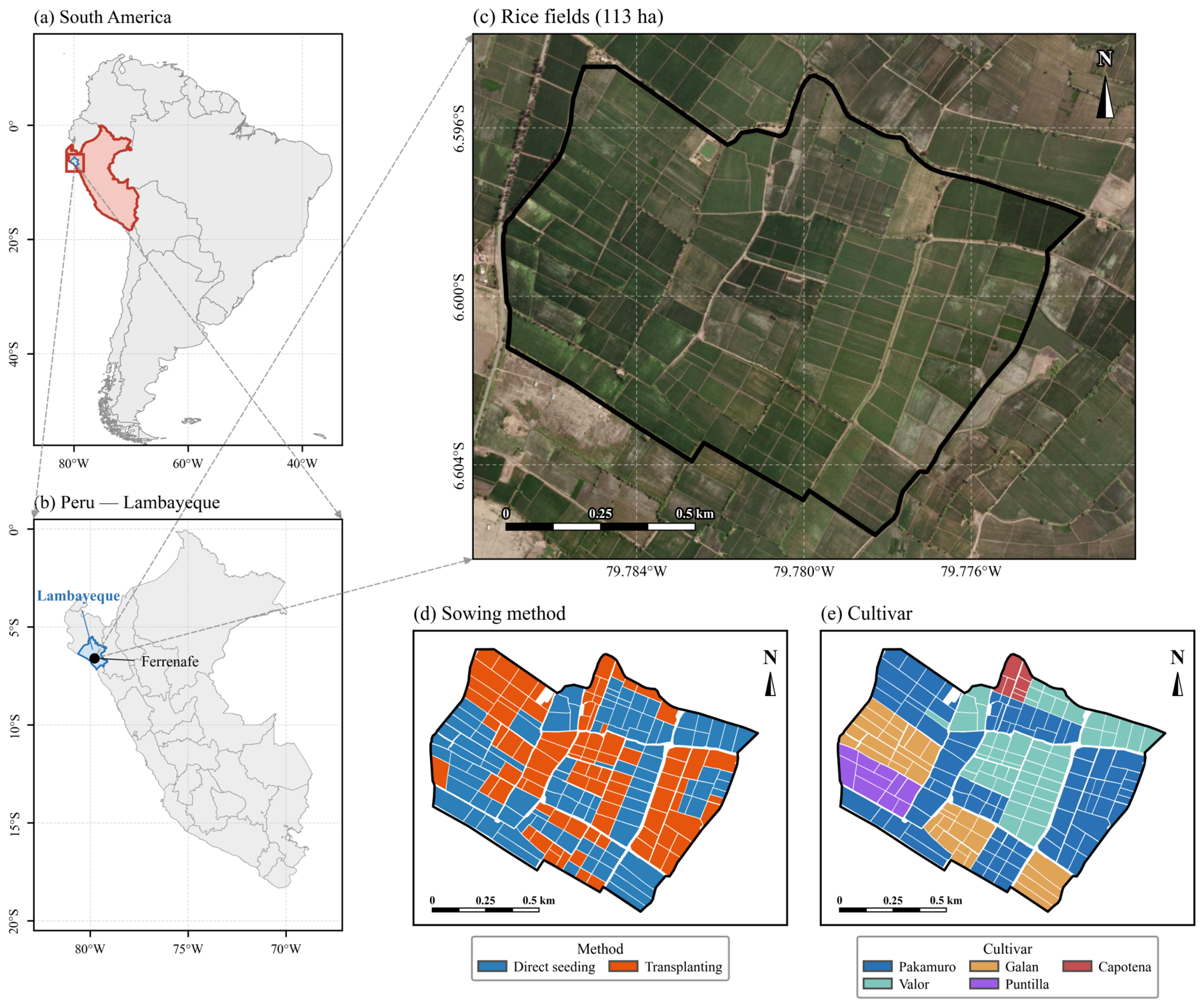
Figure 1. Study area: a flood-irrigated rice block on the arid northern coast of Peru. The figure locates the site and documents the two management attributes against which the spatial variability of ET is later tested. (a) Peru within South America; (b) Ferreñafe District (Lambayeque); (c) the 113 ha rice block, the region of interest (ROI), with the Vista Florida station of the National Institute for Agricultural Innovation (INIA) ∼14 km south; (d) parcels by sowing method; (e) parcels by cultivar. Lambayeque is the leading rice-producing region of Peru, receives about 22 mm of rainfall a year so that the crop depends entirely on irrigation, and is almost cloud-free, which is what makes a ten-date Landsat series possible in one season. Panel (c) basemap: Esri, Maxar, Earthstar Geographics.
Remotesensing 18 02584 g001
Figure 2. Meteorological forcing and its in situ corroboration. The figure documents the evaporative demand that drives the energy balance on each date and how far the reanalysis used as forcing departs from the observations recovered on the ground. (a) ERA5-Land forcing over the ten dates (daily reference evapotranspiration E T o as bars; air temperature T a i r and incoming solar radiation R s divided by 100 at overpass) with the quality-controlled station observations overlaid ( E T o , diamonds; daily-mean air temperature, circles). (b) Hourly FAO-56 E T o at the station for the six recovered dates; the grey band marks the approximate Landsat overpass, at which the instantaneous reference E T o , inst used in the METRIC internal calibration is taken. Station–ERA5-Land agreement is quantified in Figure S10 and Table S11.
Remotesensing 18 02584 g002
Figure 3. Four-stage processing workflow of the METRIC implementation on Google Earth Engine. The diagram shows what is computed, in which order, and on which platform; every block is described in the text. (1) Input data (Landsat 8/9 OLI/TIRS, that is, the Operational Land Imager and the Thermal Infrared Sensor, the Shuttle Radar Topography Mission (SRTM) digital elevation model, and ERA5-Land); (2) pre-processing in Google Earth Engine (radiometric calibration and albedo, vegetation indices and leaf area index (LAI), surface temperature and emissivity); (3) the surface energy balance solved in Python, with the anchor pixels selected automatically by the CIMEC algorithm (Calibration using Inverse Modeling at Extreme Conditions) [33] within the METRIC internal calibration framework [12], and the sensible heat flux H obtained by Monin–Obukhov iteration; and (4) the daily evapotranspiration ( E T 24 h = E T r F · E T o , 24 h ), its comparison against FAO-56, and the spatial analysis by sowing method and cultivar. Box colours follow the legend; solid arrows denote the processing flow, and dotted arrows indicate the ET retrieval and its evaluation. The four grey rounded boxes delimit the four stages, and the green dotted outline around the daily ET box marks the main product of the workflow, the 30 m ET raster on which every result reported below is based.
Remotesensing 18 02584 g003
Figure 4. Timeline of the 2022 campaign. The figure places every experimental step on a common time axis, so that the phenological stage, the imagery, and the meteorological source available on any date can be read together. (a) Crop calendar with the five phenological stages, the ten Landsat 8/9 overpasses by satellite, and the availability of the two meteorological sources: ERA5-Land is continuous, whereas the Vista Florida station has no record for May and lacked a pyranometer and anemometer from January to April, so its reference evapotranspiration ( E T o ) was recovered on only six of the ten dates. The scene set aside by the quality control of Section 2.5.1 (5 May) is crossed out. (b) FAO-56 crop coefficient K c per stage against days after sowing, with each acquisition on its step. The K c = 1.10 step was never applied, because no cloud-free scene fell in that window.
Remotesensing 18 02584 g004
Figure 5. Surface variables retrieved over the ROI at full canopy cover (10 March 2022). The panels show the spatial texture of the four inputs that drive the energy balance on a representative mid-season date: the canopy is closed and fairly uniform, the coolest surfaces coincide with the densest canopy and standing water, and the sharpest contrasts sit at the field edges and in the parcels established later. This is the pattern that later appears in the ET maps. (a) Normalised difference vegetation index (NDVI); (b) leaf area index (LAI); (c) surface temperature ( T s ), derived from a thermal observation acquired at 100 m and resampled to the 30 m grid; and (d) albedo. ROI, region of interest, the 113 ha rice block. Black line, field boundary; grey lines, individual parcels.
Remotesensing 18 02584 g005
Figure 6. Properties of the anchor pixels selected automatically on each date. The internal calibration of METRIC rests entirely on these two pixels, so the figure is the visual check that the automatic rule found a genuine thermal and vegetation contrast on every date. A wide separation in both panels indicates well-conditioned calibration; the narrow separation on 5 May is what the quality control described in Section 2.5.1 detects. Anchor pixels selected by the CIMEC algorithm (Calibration using Inverse Modeling at Extreme Conditions) per date: (a) surface temperature T s of the cold and hot anchors, labelled with the thermal contrast Δ T s ; (b) their normalised difference vegetation index (NDVI).
Remotesensing 18 02584 g006
Figure 7. Surface energy balance components over the ROI at full canopy cover (10 March 2022). The latent heat flux in panel (d) is the residual from which ET is computed: it peaks over the dense-canopy, well-flooded parcels, while the sensible heat flux rises at the edges and in the lower-cover parcels where exposed soil warms the air. (a) Net radiation R n ; (b) soil heat flux G; (c) sensible heat flux H; and (d) latent heat flux L E , all in W m−2. ROI, region of interest, the 113 ha rice block. Black line, field boundary; grey lines, individual parcels.
Remotesensing 18 02584 g007
Figure 8. Seasonal course of the field-mean ET retrieved by METRIC, with NDVI. The figure is the answer to the first objective of the study. Plotting ET against the vegetation index makes the central result visible: the highest water use occurs in January 2022, during flooding and establishment, when NDVI is still low, so evaporation from the free water layer, rather than canopy transpiration, likely governs ET at that stage. This decoupling is what a tabulated crop coefficient, which follows the canopy, cannot reproduce. Daily field-mean evapotranspiration (ET, blue line; shaded band, the spatial minimum to maximum range across the field) and mean normalised difference vegetation index (NDVI, green line) over the 2022 season. The background shading indicates the approximate phenological stages.
Remotesensing 18 02584 g008
Figure 9. Daily ET maps over the ROI for the ten Landsat dates. The maps carry the two results that a point-wise crop coefficient cannot provide: the seasonal decline from flooding in January to harvest in July, and a spatial heterogeneity within the block that persists on every date (coefficient of variation of 6 to 14%; Figure S11). It is this within-field structure, rather than the difference between management groups, that dominates the variability of water use. Daily evapotranspiration (ET, mm d−1) on a common colour scale. ROI, region of interest, the 113 ha rice block. Black line, field boundary; grey lines, individual parcels. Scale bar and north arrow in the first panel.
Remotesensing 18 02584 g009
Figure 10. Comparison of E T METRIC with the FAO-56 reference. The figure identifies the crop stages at which the two approaches agree and those at which they diverge. Both estimates share the same reference E T o , so the panels show consistency between two modelling approaches rather than validation against measured ET. (a) Shown is 1:1 scatter vs. E T F A O - 56 ( K c E T o , 24 h ), points coloured by month (dashed 1:1 line; grey ±20% band); the metrics use the nine dates that passed the quality control and 5 May (open cross) is excluded (Section 2.5.1). (b) METRIC effective crop coefficient ( E T r F = E T METRIC / E T o , 24 h , Equation (6)) vs. the tabulated FAO-56 K c ; both are dimensionless and defined against the same grass E T o , so they are directly comparable.
Remotesensing 18 02584 g010
Figure 11. Distribution of the season-mean ET per parcel by management group. The figure addresses the third objective. The wide overlap between the distributions is the result: neither the sowing method nor the cultivar separates the parcels, and the spread within each group is larger than the distance between group medians. The statistically significant difference among cultivars reported in Table 7 is therefore agronomically minor. Season-mean evapotranspiration (ET) per parcel by (a) sowing method and (b) cultivar. Boxes, the interquartile range (25th to 75th percentile); line, the median; whiskers, 1.5 times the interquartile range (IQR); grey circles, individual parcels (outliers beyond 1.5 IQR omitted; the number of parcels n per group is indicated).
Remotesensing 18 02584 g011
Figure 12. Season-mean ET projected onto the parcels by management group. Filling each parcel with its group mean produces an almost uniform field, which shows that the management grouping explains little of the spatial variability seen in the per-date maps of Figure 9. Groups are distinguished by fill colour (fill and colour bar give the evapotranspiration (ET) value in mm d−1) and identified in the legend by a swatch of their mean-ET colour: (a) sowing method and (b) cultivar. The colour scale spans the group-mean range so that the small between-group differences are visible; the per-parcel distributions are in Figure 11 and Table 7. The legend reports each group’s mean ± standard deviation. Field outlined in grey; thin lines, parcel boundaries; scale bar and north arrow in panel (a).
Remotesensing 18 02584 g012
Table 1. Landsat 8/9 scenes processed for the 2022 rice season. These ten acquisitions define the temporal sampling of the whole study: every ET map, calibration, and comparison reported below is derived from them, and their spacing is what limits the temporal resolution of the seasonal series. Scenes over Ferreñafe (path/row 10/65), all cloud-free over the region of interest (ROI). Cloud cover is the fraction screened pixel by pixel inside the ROI rather than over the whole scene. The reflective bands are acquired at 30 m and the thermal band at a native 100 m resampled onto the same 30 m grid (Section 2.2). L8, Landsat 8; L9, Landsat 9.
DateSensorPath/RowCloud ROI (%)
13 January 2022L910/650
29 January 2022L910/650
10 March 2022L810/650
3 April 2022L910/650
5 May 2022L910/650
21 May 2022L910/650
29 May 2022L810/650
14 June 2022L810/650
22 June 2022L910/650
8 July 2022L910/650
Table 2. Seasonal course of the retrieved surface variables. These four variables are the inputs from which the energy balance is solved, so their seasonal behaviour is what drives the ET dynamics reported later; the table also shows that the retrievals follow crop phenology, which is the first consistency check on the model. Spatial means over the region of interest (ROI, 113 ha) per date: the normalised difference vegetation index (NDVI), the leaf area index (LAI), the surface temperature ( T s ), and the albedo. These are the four variables mapped for the representative full-cover date in Figure 5; their multi-date evolution and intra-field distribution are given in the Supplementary Materials.
DateNDVI
(–)
LAI
(m2 m−2)
Ts
(°C)
Albedo
(–)
13 January 20220.180.0030.00.11
29 January 20220.350.2026.80.11
10 March 20220.690.9825.80.14
3 April 20220.681.0423.80.16
5 May 20220.470.5422.60.19
21 May 20220.320.2428.10.19
29 May 20220.310.2227.40.19
14 June 20220.270.1528.70.18
22 June 20220.230.0829.70.15
8 July 20220.210.0532.50.15
Table 3. METRIC internal calibration coefficients per date. The two automatically selected anchor pixels fix the calibration of the sensible heat flux on each date, so these coefficients and the thermal contrast behind them are the primary diagnostic of how trustworthy each scene is. The 5 May date stands out with the steepest slope and the weakest contrast, which is why it is set aside by the quality control of Section 2.5.1. Coefficients a (slope) and b (intercept) are of the calibration function d T = a T s + b , where d T is the near-surface temperature gradient and T s the surface temperature; cold–hot thermal contrast Δ T s (in K; for a temperature difference, 1 K ≡ 1 °C); and the number of Monin–Obukhov stability iterations (Iter.).
Dateab Δ T s (K)Iter.
13 January 20220.084−21.413.320
29 January 20220.141−39.213.420
10 March 20220.145−40.414.320
3 April 20220.126−33.713.020
5 May 20220.355−101.97.720
21 May 20220.208−59.010.820
29 May 20220.201−56.810.420
14 June 20220.166−46.010.520
22 June 20220.195−55.19.020
8 July 20220.164−45.711.420
Table 4. Seasonal course of the surface energy balance components. The latent heat flux in the last column is the residual from which ET is obtained, so this table shows how the available energy is partitioned through the season and why ET declines towards harvest: net radiation falls while the sensible heat flux rises. Spatial means over the region of interest (ROI, 113 ha) per date: net radiation ( R n ), soil heat flux (G), sensible heat flux (H), and latent heat flux ( L E ). All components are expressed in W m−2.
Date R n GHLE
(W m−2)
13 January 2022655110166380
29 January 2022677107124447
10 March 2022656103147408
3 April 202262596199330
5 May 202255995138326
21 May 202250893150265
29 May 202250792175240
14 June 202248993204192
22 June 202249795155247
8 July 202249399157237
Table 5. Daily field-mean evapotranspiration retrieved by METRIC. This is the main product of the study: the highest ET occurs during flooding at low NDVI, when the free water layer rather than the canopy governs evaporation. Daily field-mean evapotranspiration (ET) per date, with the mean normalised difference vegetation index (NDVI) and leaf area index (LAI) over the region of interest (ROI) and the approximate phenological stage. SD, spatial standard deviation of daily ET across the field (mm d−1); ET range, intra-field minimum to maximum. The maximum ET value is shown in bold.
DateNDVILAIET MeanSDET RangeStage
(m2 m−2)(mm d−1)
13 January 20220.180.007.940.735.39–9.76Establishment
29 January 20220.350.208.130.566.08–9.49Establishment
10 March 20220.690.987.020.475.92–8.98Mid-season (flowering)
3 April 20220.681.045.990.345.13–7.83Mid-season (flowering)
5 May 20220.470.545.560.493.75–6.94Maturation
21 May 20220.320.244.510.483.21–5.86Maturation
29 May 20220.310.224.150.572.66–6.16Maturation
14 June 20220.270.154.270.562.12–6.33Post-harvest
22 June 20220.230.085.040.643.11–6.68Post-harvest
8 July 20220.210.054.860.493.36–6.63Post-harvest
Table 6. Comparison of E T METRIC with the FAO-56 reference, by date. The table identifies the stages at which the two approaches agree and those at which they diverge. Both are built on the same reference E T o , so the statistics measure consistency between two modelling approaches, not accuracy against measured ET. E T METRIC against E T F A O - 56 = K c E T o , 24 h ( E T o , 24 h integrated from 24 hourly ERA5-Land values; K c , tabulated FAO-56 crop coefficient for flooded rice, dimensionless). Diff. = E T METRIC E T F A O - 56 (mm d−1); positive means METRIC gives the higher estimate. RMSE, root mean square error; MAE, mean absolute error; MBE, mean bias error; PBIAS, percent bias; r 2 , squared Pearson correlation. 5 May is excluded by the quality control described in Section 2.5.1; the all-dates values are given alongside so the effect of that decision is visible.
Date K c ETo,24hETFAO-56ETMETRICDiff.Diff. (%)
(–)(mm d−1)(mm d−1)(%)
13 January 20221.055.445.727.94+2.22+38.9
29 January 20221.056.356.678.13+1.46+21.9
10 March 20221.206.487.777.02−0.75−9.7
3 April 20221.205.436.515.99−0.52−8.0
5 May 2022 0.953.573.395.56+2.17+63.9
21 May 20220.954.624.394.51+0.12+2.7
29 May 20220.954.714.484.15−0.33−7.3
14 June 20220.904.343.914.27+0.36+9.3
22 June 20220.804.153.325.04+1.72+51.6
8 July 20220.754.383.294.86+1.57+47.9
Excluding 5 May ( n = 9 ): RMSE = 1.23, MAE = 1.01, MBE = +0.65 mm d−1, PBIAS = +12.7%, r 2 = 0.57. All dates ( n = 10 ): RMSE = 1.35, MAE = 1.12, MBE = +0.80 mm d−1, PBIAS = +16.2%, r 2 = 0.53.
Table 7. Season-mean ET by sowing method and by cultivar. The table answers the third objective of the study, and its result is negative in a useful way: the contrast between management groups is far smaller than the intra-field variability of Table 5, which is what indicates that water use here responds to water management and local phenology rather than to sowing method or cultivar. Season-mean evapotranspiration (ET, mm d−1, area-weighted mean of the ten dates) obtained by overlaying the 189-parcel map with the ET rasters. n, number of parcels in each group; SD, standard deviation across parcels; the p-values come from the Mann–Whitney test between sowing methods and the Kruskal–Wallis test among cultivars. The two rows set in italics, “Sowing method” and “Cultivar”, are block headings that identify the grouping factor of the data rows below them; they carry no data.
GroupArea (ha)Mean ET (mm d−1)
Sowing method
Direct seeding55.55.73
Transplanting48.55.81
Cultivar
Pakamuro50.35.75
Valor25.75.93
Galán18.95.61
Puntilla6.55.73
Capoteña2.45.69
Disclaimer/Publisher’s Note: The statements, opinions and data contained in all publications are solely those of the individual author(s) and contributor(s) and not of MDPI and/or the editor(s). MDPI and/or the editor(s) disclaim responsibility for any injury to people or property resulting from any ideas, methods, instructions or products referred to in the content.