Analysis of Diagnostic Absorption Troughs in Clay Alteration Within the Xiangshan Uranium Deposit Based on ZY1-02E Satellite Hyperspectral Imagery

Highlights

What are the main findings?

• Based on hyperspectral remote sensing, algorithms were designed to quantitatively extract and analyze the diagnostic absorption troughs of the reflectance spectra of clay-altered minerals.
• Based on the distribution characteristics of clay alteration and the regional geology of the Xiangshan area, nine prospective mineral exploration zones have been identified.

What are the implications of the main findings?

• This demonstrates the effectiveness of hyperspectral data in the quantitative identification of altered minerals and in mineral exploration prediction.
• This can provide a reliable remote sensing basis for deep exploration of the Xiangshan uranium deposit and similar volcanic-type uranium deposits.

Abstract

The Xiangshan Uranium Deposit located in Jiangxi Province represents the largest volcanic-hosted uranium deposit in Asia and serves as a critical uranium production base in China. Clay alteration serves as a key prospecting indicator for this deposit, and its quantitative characterization through high-resolution spectroscopy is crucial for elucidating the relationship between hydrothermal activity and uranium mineralization. Addressing the current shortcoming in hyperspectral alteration mapping—which primarily focuses on qualitative mineral identification while lacking systematic quantitative characterization of diagnostic absorption trough parameters—this study utilized ZY1-02E (Chinese Resource Satellite-1-02E) satellite hyperspectral imagery as the data source. Following preprocessing, key parameters of the diagnostic absorption trough at 2205 nm for clay-altered minerals—including depth, area, and symmetry—were quantitatively extracted to construct a spectral index reflecting the intensity of clay alteration. Subsequently, the spatial distribution characteristics of these parameters were systematically analyzed. It was found that, with the line connecting Yankeng, Youjiashan, Xiangshan, and Yunji serving as a boundary, clay alteration generally exhibits a distribution trend of being stronger in the northwest and weaker in the southeast, with morphological features characterized by a combination of strip-like, ring-shaped, and nodular patterns. Based on these findings, nine prospective exploration areas were delineated, including five Class-I and four Class-II prospective exploration areas. High-value anomalies in the absorption trough parameters show good spatial correlation with known uranium deposits and fault structures, effectively indicating the centers of hydrothermal alteration and fluid migration pathways. This study advances the remote sensing identification of clay alteration from qualitative mapping to the quantitative analysis stage, providing a scientific basis for further exploration in the Xiangshan mineralized area. The established method is highly applicable to similar volcanic-type uranium mineralized areas.

1. Introduction

The Xiangshan Uranium Ore Field in Jiangxi is China’s largest volcanic-type uranium ore field, and its formation is strongly associated with active volcanic processes, a complex tectonic setting, and multiphase hydrothermal alteration events [1,2]. To date, 31 uranium deposits have been identified in this field, predominantly concentrated in northern and western sectors of the Xiangshan Volcanic Basin, with only the Yunji deposit located in the eastern part. The host lithologies of these deposits exhibit intense alteration with diverse alteration types. Among them, clay alteration is widely distributed and relatively typical, serving as one of the key prospecting indicators in the region [3]. The Xiangshan uranium deposit experienced multistage magmatic intrusions and volcanic eruptions during Mesozoic tectonic evolution. During the late stage, large-scale fluid circulation driven by magmatic hydrothermal activity triggered intense alteration of the host rock, as well as the activation, migration, and precipitation of uranium. As a key product of this magmatic-hydrothermal mineralization process, clay alteration records changes in the physicochemical conditions of hydrothermal fluids through its mineral assemblages and reflectance spectral characteristics. Therefore, quantitative analysis of its spectral characteristics provides important guidance for reconstructing the evolution of mineralizing fluids and delineating uranium-enriched zones [4,5].

However, the use of traditional geological prospecting methods for mapping surface host rock alteration has several drawbacks, including high costs, low efficiency, and an inability to provide quantitative descriptions; these challenges are particularly acute in areas with vegetation cover. Hyperspectral remote sensing, with its integrated mapping and spectral analysis capabilities, can detect subtle spectral differences caused by mineral group vibrations, providing an effective means for the quantitative identification of altered minerals [6,7,8]. In recent years, domestically produced hyperspectral satellites, such as the ZY1-02D/02E and GF-5, have been launched one after another, providing a stable and reliable data source for large-scale, high-efficiency mineral mapping and prospecting [9,10]. Compared to multispectral remote sensing, hyperspectral remote sensing offers higher spectral resolution and is capable of detecting subtle spectral differences caused by the vibrations of mineral ions and functional groups. This enables accurate identification of the diagnostic absorption trough generated by the Al-OH bond vibration near 2205 nm, which serves as the key spectral basis for distinguishing clay alteration minerals such as kaolinite, illite, and montmorillonite [5,11]. Previously, extensive remote sensing interpretation of host rock alteration has been conducted within the Xiangshan mining district. Methods such as Principal Component Analysis (PCA), Spectral Angle Mapper (SAM), and Mixture Tuned Matched Filter (MTMF) have been widely applied in the extraction of alteration minerals and the study of mineralization zoning [12,13,14,15,16,17]. These studies primarily focused on the identification and spatial zoning of different types of host rock alteration, confirming the effectiveness of hyperspectral imaging in mapping alteration at Xiangshan and revealing patterns such as the annular distribution of alteration and the “acidic above, basic below” pattern [5,18,19,20,21,22].

However, current research still lacks systematic quantitative extraction and analysis of the morphological parameters of diagnostic absorption troughs in clay-altered minerals (such as absorption depth, area, and symmetry). These parameters are directly controlled by mineral crystallinity, relative abundance, and alteration intensity; they contain key information regarding the intensity of hydrothermal activity, the duration of fluid action, and hydrothermal–rock reaction processes, and may be closely related to remote sensing spectral characteristics and uranium mineralization potential. To date, no studies have investigated the quantitative spatial variations in diagnostic absorption trough parameters or their indicative significance for uranium mineralization at the scale of the Xiangshan uranium deposit. This gap not only limits the objective quantitative evaluation of clay alteration intensity but also hinders the transition from qualitative detection to quantitative assessment in mineral exploration prediction using hyperspectral remote sensing.

To this end, this study focuses on the Xiangshan Uranium Deposit as the research area and utilizes ZY1-02E satellite hyperspectral imagery to quantitatively extract parameters such as the depth, area, and symmetry of the diagnostic 2205 nm absorption trough associated with clay alteration. The study analyzes the spatial distribution patterns of these parameters, reveals their spatial relationships with fault structures and known uranium deposits (sites), and explores the indicative significance of these spectral parameters for hydrothermal alteration processes and uranium migration and enrichment, thereby delineating prospective exploration zones. The research findings not only provide new quantitative remote sensing evidence for the next phase of exploration in the Shangshan uranium field but also are expected to offer a replicable and scalable technical approach for quantitative hyperspectral exploration of volcanic-type uranium deposits. Additionally, they provide a spectroscopic basis for a deeper understanding of the alteration response within the magmatic-hydrothermal mineralization system in this region.

2. Geological Overview of the Study Area

2.1. Tectonic Setting

The Xiangshan Uranium Ore Field is situated at the boundary between Le’an County and Chongren County within Fuzhou City, Jiangxi Province, China. Tectonically, the ore field lies within the Xiangshan Volcanic Basin along the northeastern margin of the Yangtze Block’s southeastern extensional zone, specifically within the Le’an–Fuzhou fault-ridge belt system. It lies approximately 50 km north of the Qinzhou–Hangzhou Convergence Zone and 15 km east of the Yingtan–Anyuan deep-seated fault system, with the Suichuan–Dexing Fault traversing the northwestern corner of the basin. This region has experienced successive Caledonian–Yangtze and Indosinian–Haixi orogenies, generating intense structural deformation, magmatism, and associated mineralization episodes. The ore-bearing zone occurs at the intersection between the NE-trending Gan–Hang volcanic belt and the NNW–SSE-striking Dawangshan–Yushan granitic belt, establishing a metallogenic framework conducive to U-polymetallic mineralization [2,23].

2.2. Stratum

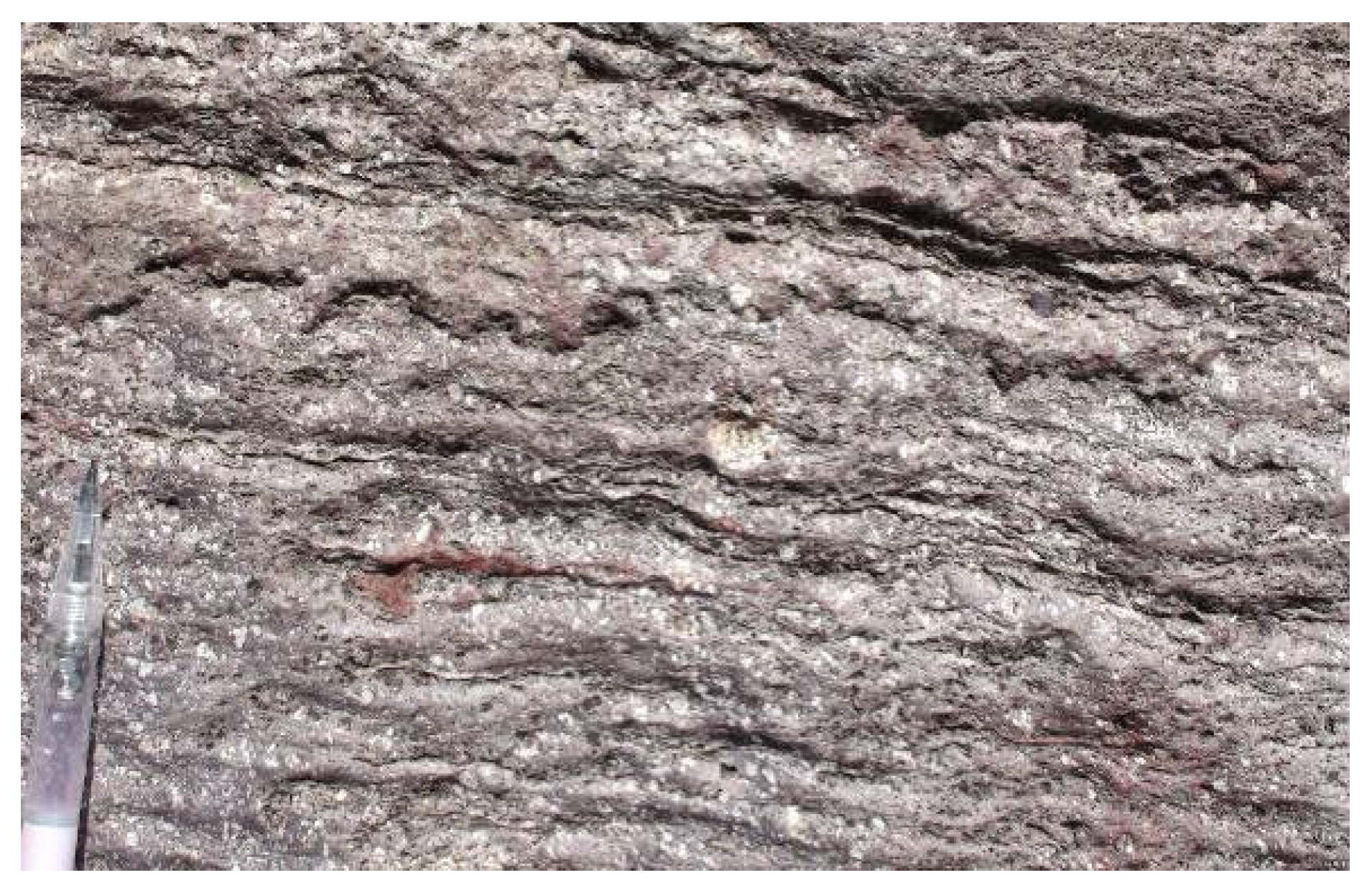
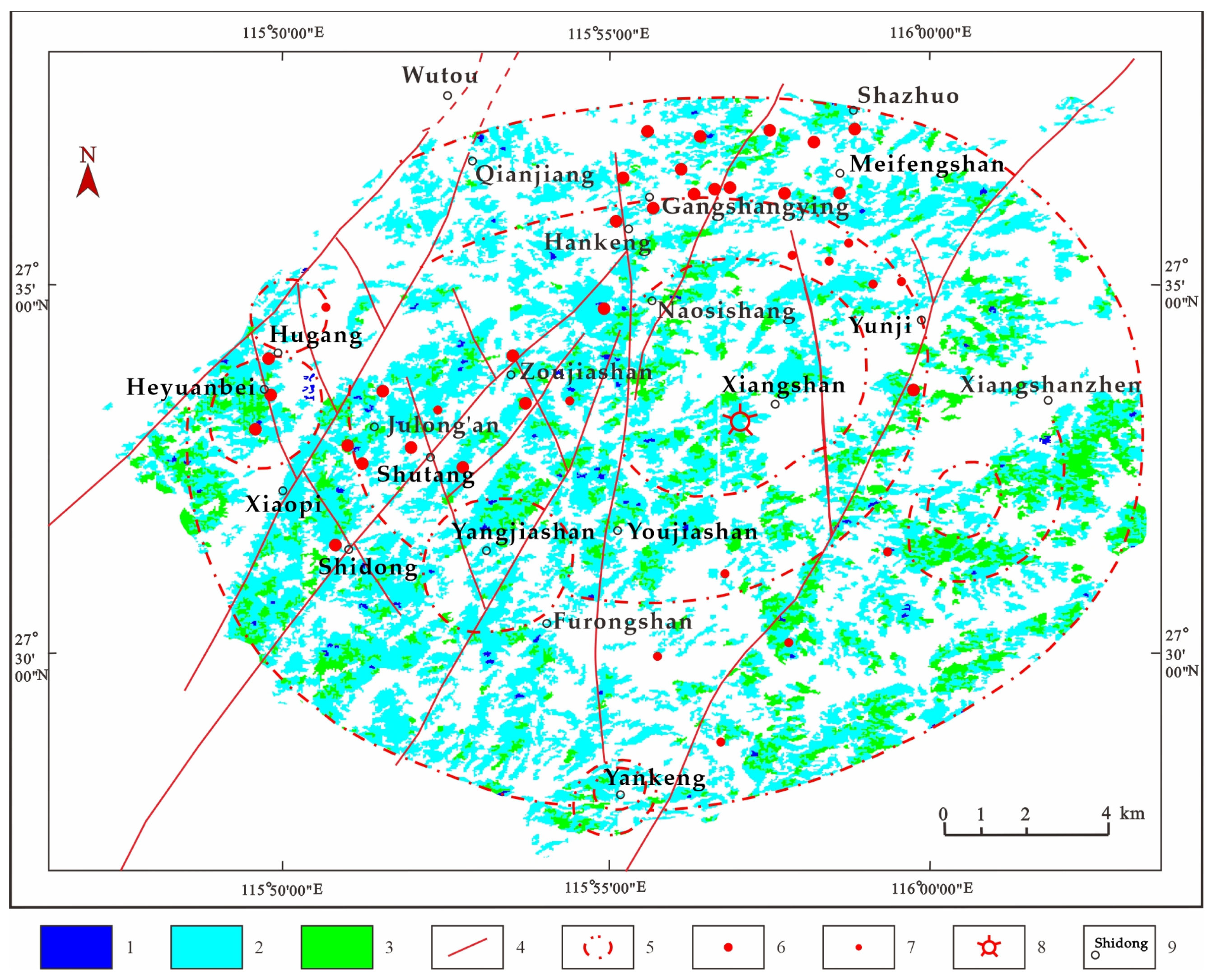
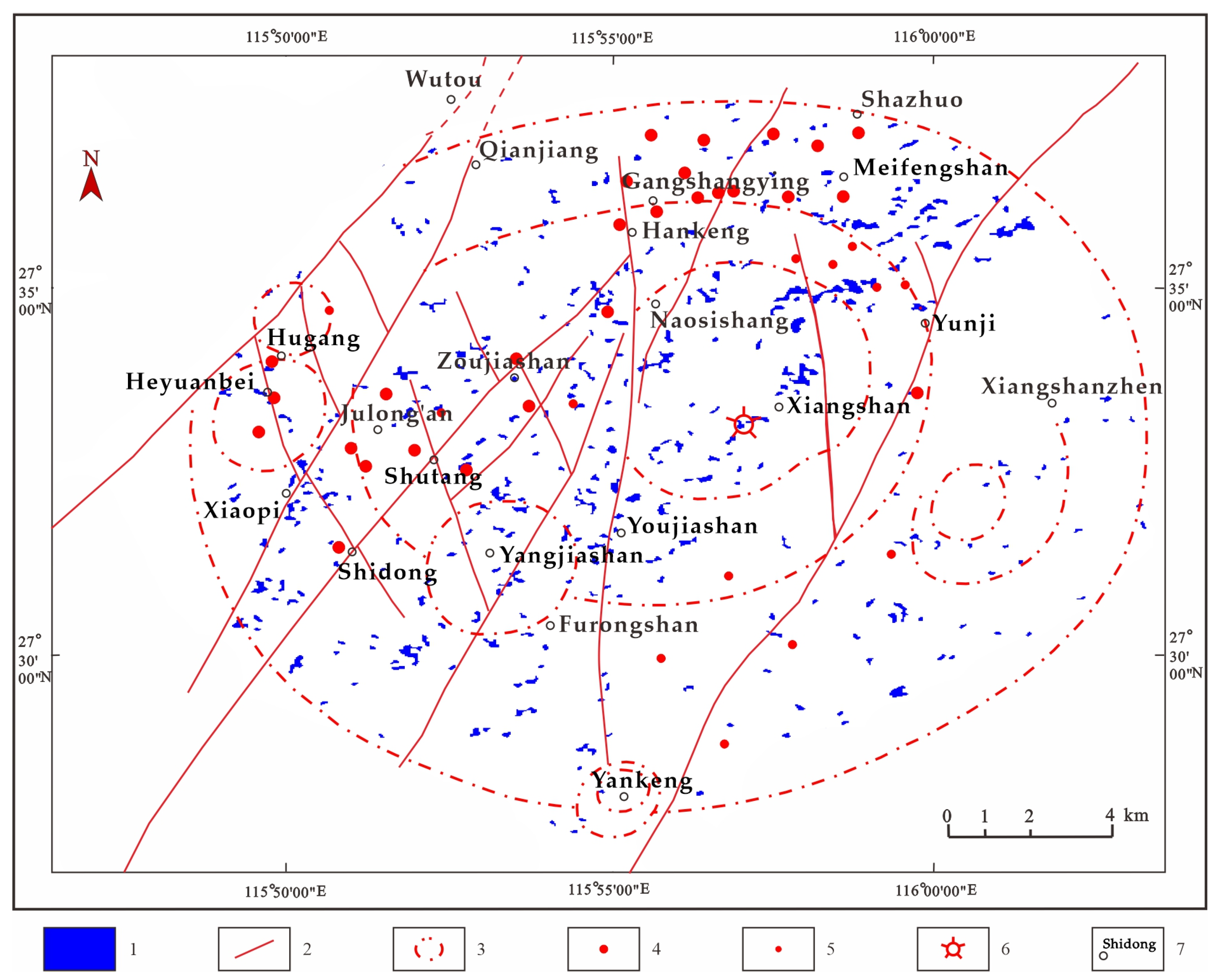
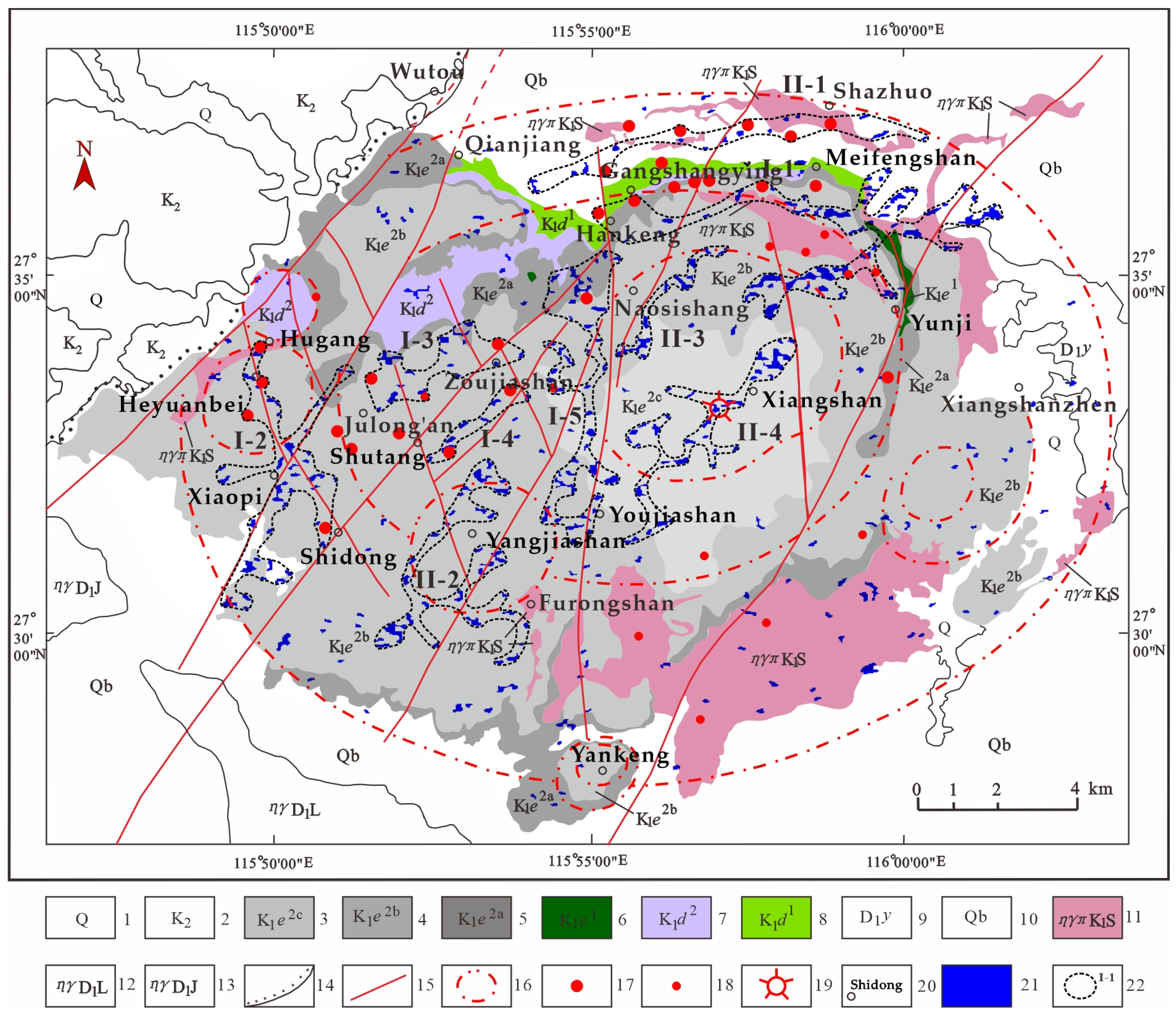
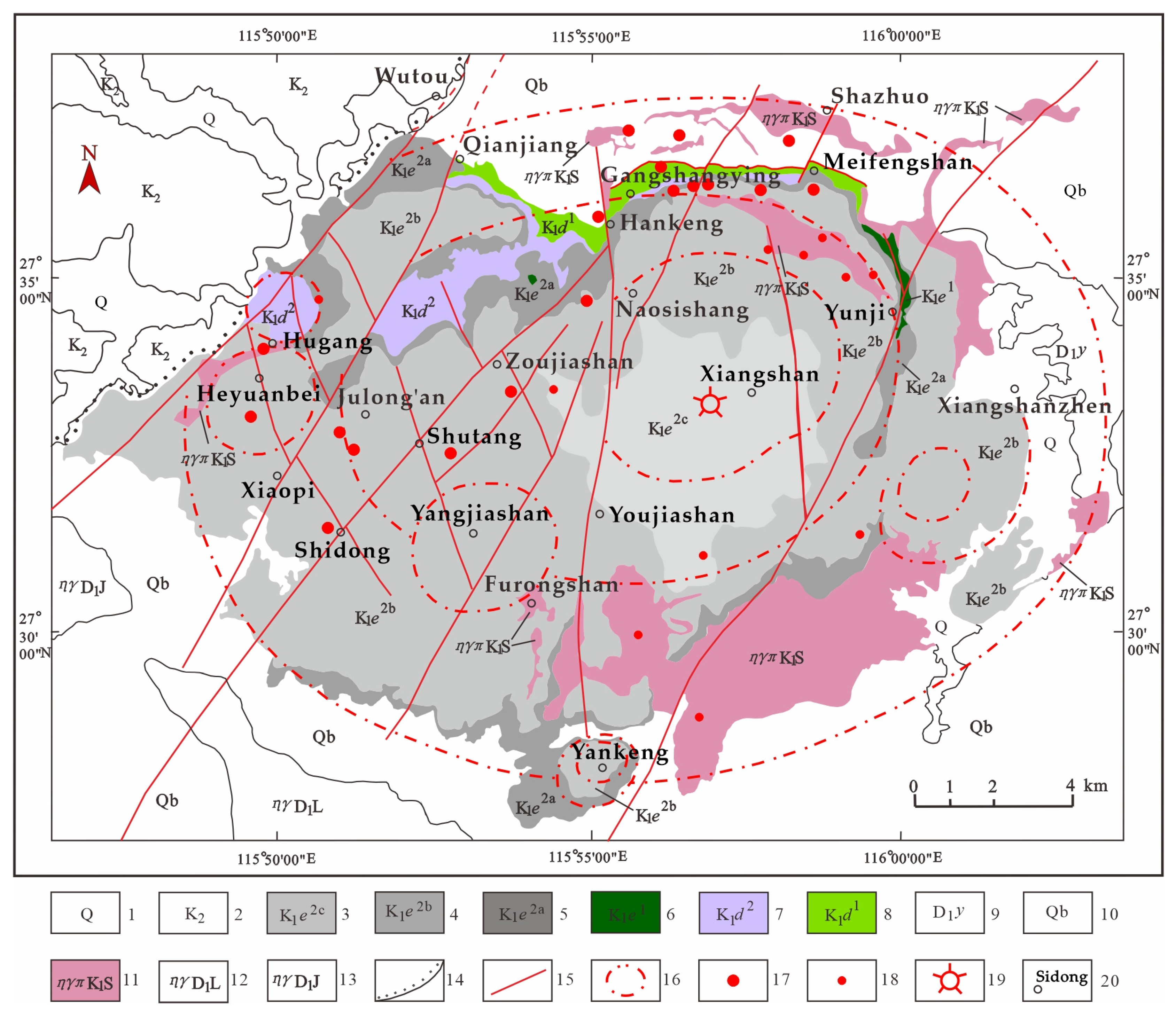
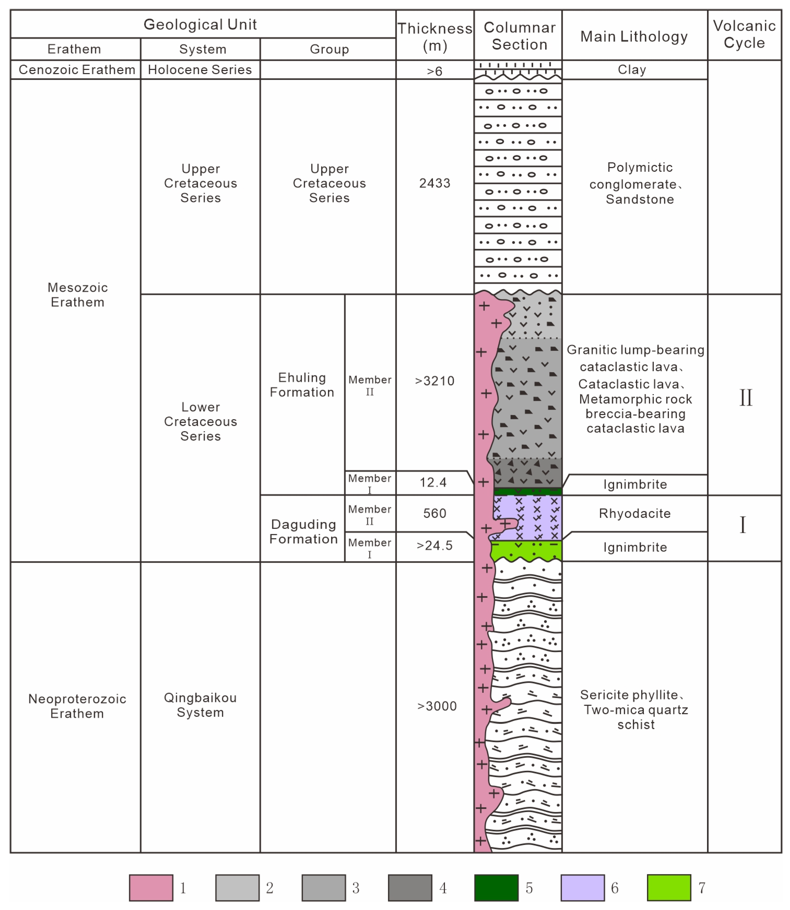
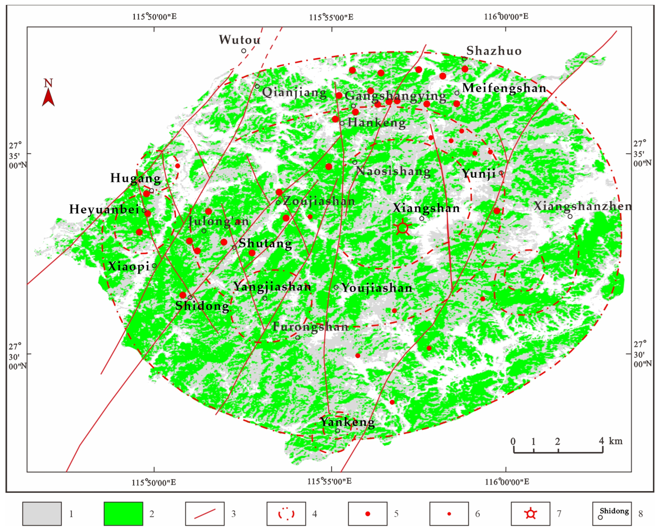
The lithostratigraphic sequence of the Xiangshan Uranium Ore Field is structurally divided into two principal components: the basement and the overlying strata. The basement strata mainly comprise the Shenshan, Kuli, and Shangshi Formations of the Qingbaikou Series, as well as the Yunsan Formation of the Lower Devonian. Metamorphic rocks assigned to the Qingbaikou System (Qb), predominantly greenschist to lower amphibolite facies (medium-low grade), crop out extensively across the study area except in its northwestern sector. This metamorphic suite comprises sericite phyllite and two-mica quartz schist displaying characteristic mineral assemblages of the greenschist-lower amphibolite facies transition [24]. The Lower Devonian Yunsan Formation (D₁y) consists primarily of conglomerates and sandstones. The overlying strata consist mainly of Mesozoic sedimentary-volcanic clastic rocks, intermediate-acidic volcanic lava, and red clastic rocks, comprising the Lower Cretaceous Daguding Formation (K₁d), the Ehuling Formation volcanic series (K₁e), and Upper Cretaceous red clastic rocks (K₂) (Figure 1 and Figure 2). The Daguding (K₁d) and Ehuling (K₁e) Formations each display distinct bipartite stratification patterns. The Daguding Formation Member I (K₁d¹) and Member I (K₁e¹) contain coherent lava flows interbedded with lapilli tuffs and volcanogenic sandstones showing graded bedding. Member II (K₁d²) is characterized by flow-banded rhyolitic lavas containing quartz phenocrysts (Figure 3). Based on lithological characteristics, the second member of the Ehuling Formation can be further subdivided into three sub-members: the marginal sub-member (K₁e^2a), the transitional sub-member (K₁e^2b), and the central sub-member (K₁e^2c), corresponding to lithologies of pyroclastic flow with metamorphic clasts, pyroclastic flow, and pyroclastic flow with granitic clasts, respectively (Figure 4).

Most rhyolite andesites exhibit a flow-banded texture, while a small number have a porphyritic texture. The rock shows significant alteration, with comb-like quartz growing on the walls of the vesicles, filled with sericite. The rock exhibits a porphyritic texture, with a phenocryst content of 10–30%. The phenocrysts consist primarily of plagioclase, potassium feldspar, biotite, and small amounts of quartz, amphibole, and pyroxene; plagioclase accounts for approximately 10–15%, with grain sizes ranging from 0.5 to 1.5 mm; potassium feldspar accounts for approximately 1–5%, with grain sizes ranging from 1 to 4 mm; quartz phenocrysts account for less than 1%, with a grain size of about 1 mm; dark minerals account for about 5%, with amphibole and biotite often exhibiting intense darkening, and pyroxene frequently altered by chlorite. The matrix exhibits a cryptocrystalline structure. It contains metamorphic brecciated basalt with a blocky texture and a brecciated structure. The phenocryst content is 50–60%, consisting primarily of potassium feldspar, quartz, plagioclase, and a small amount of biotite. Phenocrysts account for more than 60% of the rock. Plagioclase is altered to varying degrees by sericite, while biotite exhibits pronounced curving and occasionally shows darkened margins. Most phenocrysts are shattered, forming a fragmented texture. The matrix is cryptocrystalline, accounting for 20–35% of the rock. The rock contains a relatively high proportion of clasts, ranging from 6% to 15%, with sizes generally between 0.5 and 10 cm. The clasts consist primarily of metamorphic rock clasts, with small amounts of tuff and rhyolite. In phaneritic lava, the total phaneritic content can account for about 60% of the total rock. The matrix is highly crystalline, consisting of feldspar, quartz, biotite, and other minerals. In porphyritic lava, the clast content is less than 8%, with the clasts primarily consisting of sandstone, tuff, and rhyolite-andesite. Granitic-included porphyritic lava is similar to porphyritic lava but exhibits a higher degree of crystallization. Its defining characteristic is the presence of granitic inclusions, which account for 5% to 15% of the rock and generally range in size from 5 to 30 cm; these inclusions are granodiorite. Additionally, the rock contains varying amounts of metamorphic rock clasts, accounting for approximately 1% to 12% of the total.

2.3. Intrusive Rock

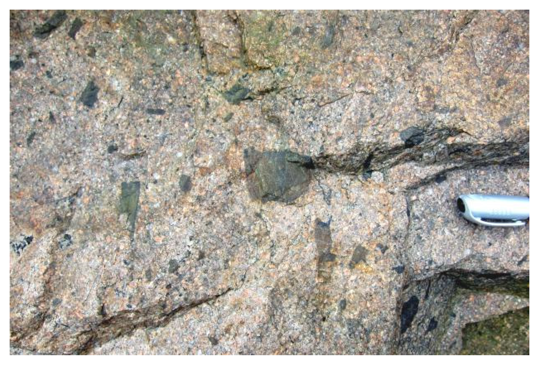
The Xiangshan Uranium Ore Field has undergone intense magmatic activity. The exposed intrusive rocks consist primarily of the Early Cretaceous Shazhou Unit (ηγπK₁S) of shallow-seated intrusions, which are coarse-grained monzogranite porphyry [1]. In addition, minor mafic dyke swarms including dolerite and gabbro occur sporadically [25].

Coarsely porphyritic diorite-granite, with a blocky texture and porphyritic structure. The phenocrysts consist primarily of potassium feldspar, quartz, plagioclase, and biotite. Potassium feldspar accounts for 10–35% of the rock, with the majority (20–30%) having grain sizes ranging from 7 mm × 10 mm to 12 mm × 30 mm; Quartz, with a content of 10–20%, has a grain size of 1–6 mm; plagioclase, with a content of 19–35%, has a grain size of (1–5) mm × 8 mm; Biotite, with a content of 5–10% and a particle size of 0.5–3 mm. The matrix has a cryptocrystalline structure, accounting for approximately 20–35% of the total, and consists of potassium feldspar, plagioclase, quartz, and a small amount of biotite.

2.4. Fault Structures

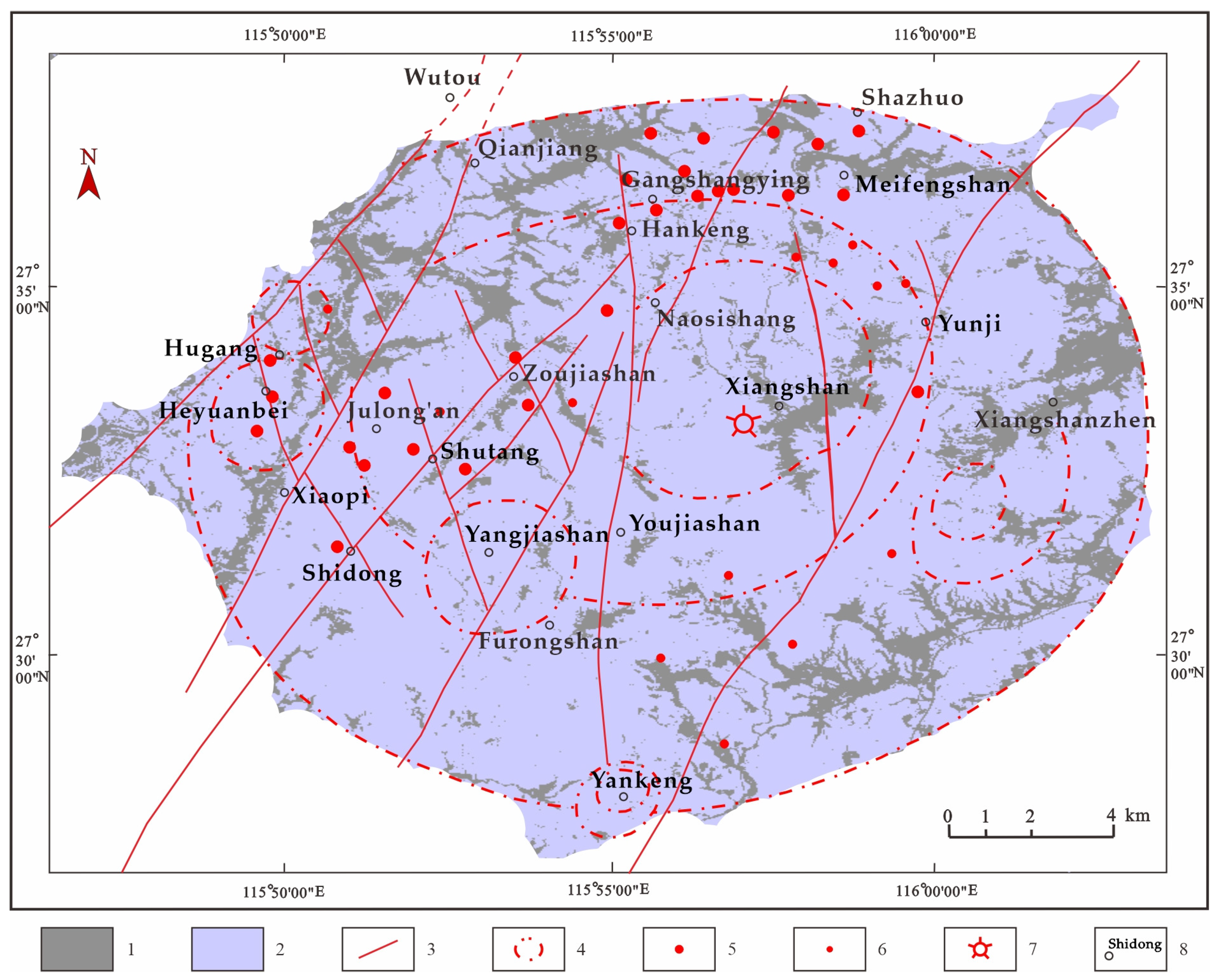
Linear structures are well-developed within the area, primarily trending NE, NW, EW, and SN. Among these, NE-trending structures are the most prominent, extending for tens of kilometers. They are predominantly left-lateral strike-slip faults, though they often exhibit some characteristics of normal faults. NW-trending faults are mostly offshoots of NE-trending faults, extending for several thousand meters. In the western part of Xiangshan, NE- and NW-trending fault structures cut through the Daguding Formation and Ehuling Formation, forming a diamond-shaped grid-like landform. SN-trending faults are less common. The largest SN-trending fault is the Hankan–Youjiashan Fault, which extends over 30 km and cuts across the entire basin [23] (Figure 1). The remaining SN-trending fault structures generally have shorter extensions and are mostly derived from NE- and NW-trending faults. The basin is controlled by large-scale collapse-type volcanic structures, resulting in the formation of numerous ring-shaped structures.

2.5. Uranium Mineralization and Host Rock Alteration

Twenty-four uranium deposits have been identified within the Xiangshan Uranium Ore Field, along with a large number of uranium prospects, mineralized zones, and mineralization anomalies (including alteration zones and geochemical halos). These uranium accumulations exhibit extensive lateral development and high ore grades, making them typical and representative of volcanic-type uranium deposits in China [26]. Based on the spatial distribution of uranium deposits and the similarities and differences in the primary controlling factors, the field can be divided into the western, northern, and eastern mining districts [27]. To date, no deposits have been discovered in the central and southern parts of the field. The Northern Mining Area accounts for 36.7% of total resource reserves, while the Western Mining Area accounts for 56.5%. Moreover, exploration results and future exploration potential in the Western Mining Area are superior to those in the Northern Mining Area [28]. The deposits in the Western and Eastern Mining Areas are of the effusive volcanic facies (VF), with rhyolite and porphyritic lava serving as the primary host rocks. While the deposits in the Northern Mining Area are hypabyssal in type, with medium-to-coarse-grained K-feldspar-plagioclase granodiorite serving as the primary host rock. The former is represented by deposits such as the Zoujia, Julong’an, Heyuanbei, and Lijialing deposits, while the latter is represented by the Hengjian–Gangsang Ying, Hongwei, and Shazhou deposits [29].

The host rocks within the mineralized area exhibit intense alteration characterized by multiple phases and stages. Alteration from different phases overlaps spatially while also displaying a certain degree of zonation. The main alteration types include sericite alteration, chlorite alteration, hematite mineralization, pyrite mineralization, muscovite alteration, fluorite alteration, carbonate alteration, and silicification. Among these, hematitization, fluoritization, and sericitization are important prospecting indicators in the area [30]. Based on the chronological sequence of alteration and its relationship with uranium mineralization, these can be broadly classified into three categories: pre-mineralization hydrothermal alteration, mineralization-phase hydrothermal alteration, and post-mineralization hydrothermal alteration [31]. Pre-mineralization host rock alteration is primarily characterized by sericite alteration, chlorite alteration, and muscovite alteration, with sericite alteration being the most intense and distributed throughout the entire mineralized area [32]. Host rock alteration during the mineralization phase can be divided into two stages: early-stage alteration dominated by hematite mineralization, and late-stage alteration dominated by fluorite, muscovite, and chlorite alteration. The early stage is also accompanied by weaker sodalite, chlorite, and muscovite alteration, while the late stage is accompanied by carbonatization and pyrite mineralization [33]. Host rock alteration during the late stage of mineralization is dominated by carbonatization, silicification, and fluorite mineralization, with a relatively small scale of alteration. In summary, hydromica alteration develops during both the early and main stages of mineralization, covering a large area with intense alteration, and thus holds significant implications for mineral exploration.

3. Introduction to ZY1-02E Satellite Hyperspectral Imagery and Data Preprocessing

3.1. Introduction to ZY1-02E Satellite Hyperspectral Data

On 26 December 2021, the ZY1-02E satellite was successfully launched from the Taiyuan Satellite Launch Center by a Long March 4C carrier rocket. As the ninth satellite in the ZY-1 series, it operates in a constellation with the ZY1-02D satellite launched in 2019, reducing the revisit cycle to two days [34]. The visible/near-infrared (VNIR) sensor and hyperspectral imager onboard the ZY1-02E satellite are similar to those carried by the ZY1-02D satellite, featuring hyperspectral and spatial resolution capabilities. These instruments provide high-quality imagery data for the interpretation of lithology, tectonics, and host rock alteration [35,36,37]. The visible/near-infrared sensor on the ZY1-02E satellite captures a total of 9 bands, including the panchromatic band B01 with a spatial resolution of 2.5 m and the multispectral bands B02–B09 with a spatial resolution of 10 m and a swath width of 115 km. The long-wave infrared camera captures only one band, with a spatial resolution of 15 m and a swath width of 115 km [38,39] (

Table 1. Band setting of ZY1-02E satellite sensor.

Sensor Type	Number of Bands	Spectral Number	Spectral Range	Resolution	Web Width
Hyperspectral imager	166	B01~B166	400~2500 nm	30 m	60 km
Visible/Near-Infrared Sensor	9	B01	452~902 nm	2.5 m	115 km
		B02	450~520 nm	10 m
		B03	520~590 nm
		B04	630~690 nm
		B05	770~890 nm
		B06	400~450 nm
		B07	590~625 nm
		B08	705~745 nm
		B09	860~1040 nm
Long-wave infrared camera	1	B01	8000~10,000 nm	15 m	115 km

). The hyperspectral imager captures a total of 166 bands, with a spectral range of 400–2500 nm, a spatial resolution of 30 m, and a swath width of 60 km. This study selected remote sensing image data from the ZY1-02E satellite, imaged on 21 November 2023, as the data source for the quantitative analysis of diagnostic absorption features associated with clay alteration in the Xiangshan Uranium Ore Field.

3.2. Data Preprocessing

The image data obtained in this study are L1-level data, which contain some striped noise. These periodic noise patterns may compromise diagnostic absorption feature extraction from hydrothermally altered minerals. Therefore, the images require processing such as bad-band removal, radiometric calibration, atmospheric correction, streak noise removal, and geometric correction. All preprocessing operations were conducted in ENVI v5.6 (Environment for Visualizing Images; Harris Geospatial Solutions, Boulder, CO, USA). The ENVI software supports key preprocessing workflows for ZY1-02E hyperspectral satellite data, including data reading, data preprocessing and pixel resampling. Its spectral resampling module enables automated continuum removal and spectral angle mapper (SAM) implementation for alteration mineral identification.

Preprocessing begins with band selection. The ZY1-02E satellite remote sensing imagery consists of 166 bands, including 76 visible and near-infrared bands with a spectral range of 386–1030 nm, and 90 short-wave infrared bands with a spectral range of 1009–2510 nm. To retain bands with a higher signal-to-noise ratio and improve the accuracy of subsequent alteration feature extraction, this study excluded 29 bands that were severely affected by water vapor, had low signal-to-noise ratios, or showed high correlation with adjacent bands, ultimately retaining 137 valid bands (

Table 2. Bad band elimination.

Type	Band	Wavelength Range (nm)
Lower signal-to-noise ratio bands	VN: 1–2	386–396
	SW: 31	1515–1516
	SW: 60–61	2003–2021
	SW: 65	2087–2088
	SW: 88–90	2475–2510
Overlapping bands	SW: 1–2	1009–1027
Periods of significant moisture influence	SW: 22–27	1363–1448
	SW: 48–57	1801–1954
	SW: 82–83	2374–2392

).

On this basis, radiometric calibration was performed to convert the raw digital number (DN) values acquired by the sensor into physically meaningful radiance values. The radiance value is calculated using the following formula:

$${\mathrm{L}}_{\mathsf{\alpha }}=\mathrm{G}\mathrm{a}\mathrm{i}\mathrm{n}·\mathrm{D}\mathrm{N}+\mathrm{O}\mathrm{f}\mathrm{f}\mathrm{s}\mathrm{e}\mathrm{t}$$

(1)

where ${\mathrm{L}}_{\mathsf{\alpha }}$ is the radiance value of the band, DN is the pixel grayscale value, gain is the calibration slope, and offset is the absolute calibration coefficient.

The computed radiance value is a floating-point number between 0 and 1. Because hyperspectral images contain a large number of spectral bands, storing floating-point data directly would consume a significant amount of storage space, resulting in very large file sizes. To standardize the data format and facilitate processing across various software applications, reflectance values ranging from 0 to 1 are typically scaled and converted to integers for storage. In this paper, the scaling factor (OGPScaleFactor) defined in the header file is set to 10,000, meaning the reflectance of the original data has been amplified by a factor of 10,000. Therefore, when calculating band reflectance, the read integer pixel values must be divided by 10,000 to restore the actual reflectance values.

Even after radiometric calibration, images remain subject to atmospheric scattering, reflection, and absorption, which distort the spectral information of ground objects. Atmospheric correction is required to obtain data that more closely reflect the actual reflectance of ground objects, thereby providing reliable image data for subsequent spectral analysis and quantitative inversion. This paper employs the FLAASH (Fast Line-of-sight Atmospheric Analysis of Spectral Hypercubes) module in ENVI software to perform atmospheric correction on ZY1-02E satellite hyperspectral imagery. FLAASH is based on the MODTRAN radiative transfer model and is capable of accurately correcting atmospheric disturbances in the visible to shortwave infrared range, making it particularly suitable for the processing of hyperspectral imagery. During the atmospheric correction process, appropriate atmospheric models and aerosol types were selected based on the image’s acquisition time, geographic location, and sensor parameters. Spectral smoothing and resampling were then performed using the ZY1-02E satellite’s band response functions. Through these steps, surface reflectance images that accurately reflect the spectral characteristics of terrestrial features were ultimately obtained. In the FLAASH model, the surface is assumed to be a standard Lambertian surface. The formula for calculating the spectral radiance of a pixel received by the sensor is as follows:

$${\mathrm{L}}_{\mathsf{\beta }}=\left({\displaystyle \frac{\mathrm{A}\mathsf{\rho }}{1-{\mathsf{\rho }}_{\mathrm{e}}\mathrm{S}}}\right)+\left({\displaystyle \frac{\mathrm{B}{\mathsf{\rho }}_{\mathrm{e}}}{1-{\mathsf{\rho }}_{\mathrm{e}}\mathrm{S}}}\right)+{\mathrm{L}}_{\mathsf{\alpha }}$$

(2)

where ${\mathrm{L}}_{\mathsf{\beta }}$ is the total radiant brightness received by the sensor pixel, $\mathsf{\rho }$ is the surface albedo of the pixel, $\mathrm{S}$ is the spherical albedo at the top of the atmosphere, ${\mathrm{L}}_{\mathsf{\alpha }}$ is the atmospheric backscatter radiance (atmospheric backscatter), $\mathrm{A}$, $\mathrm{B}$ are two independent coefficients dependent on atmospheric and geometric conditions, and ${\mathsf{\rho }}_{\mathrm{e}}$ is the average surface albedo of the surrounding pixels.

The various parameters of the ZY1-02E satellite used in this paper can be obtained from the image header file; see

Table 3. FLAASH model parameters.

Parameter	Value
Sensor Type	Unknown-HSI
Sensor Height	778 km
Central Longitude and Latitude	27°43′23.81″N
	115°54′6.68″E
Duration	21 November 2023 3:21:36
Atmospheric Model	Mid-Latitude Summer
Water Vapor Inversion Occurring	Yes
Aerosol Model	Rural
Aerosol Inversion	2-Band (K-T)

for details on each parameter.

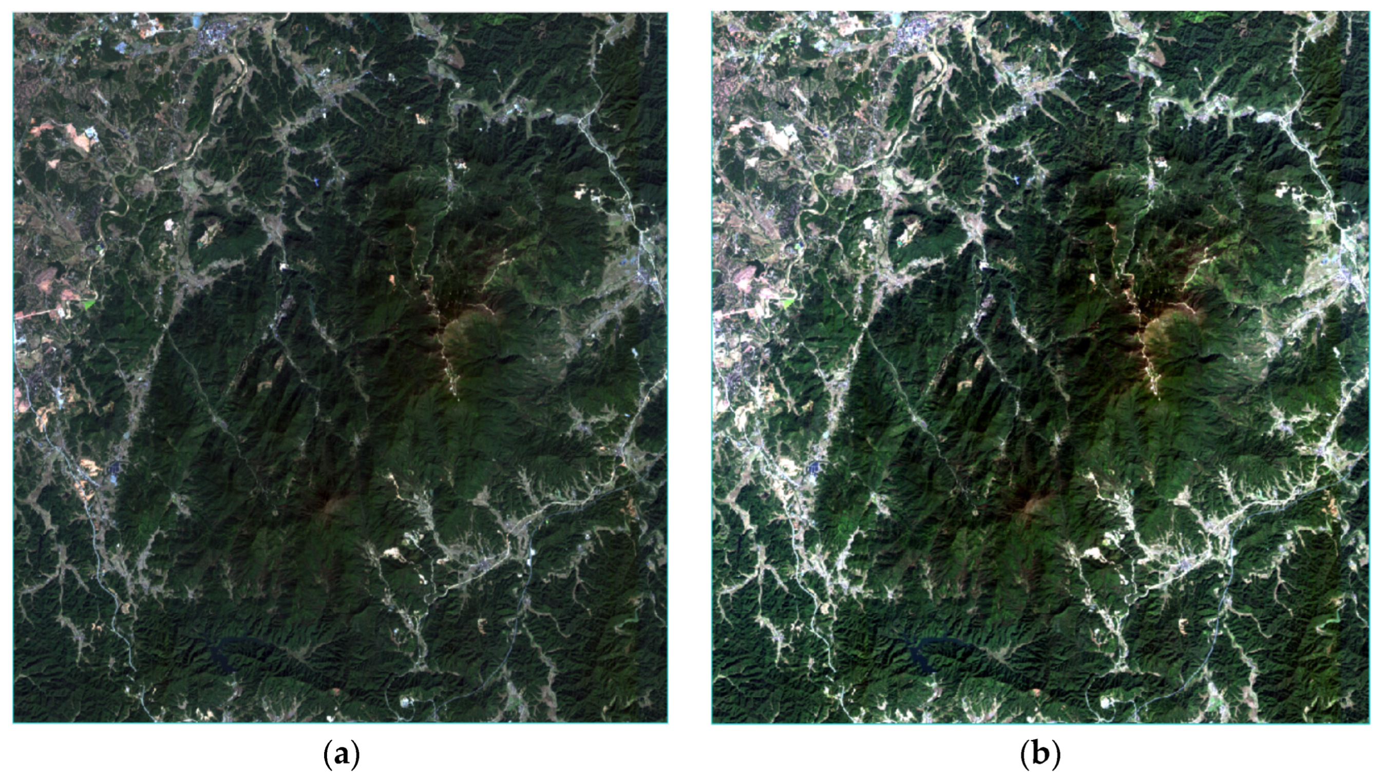
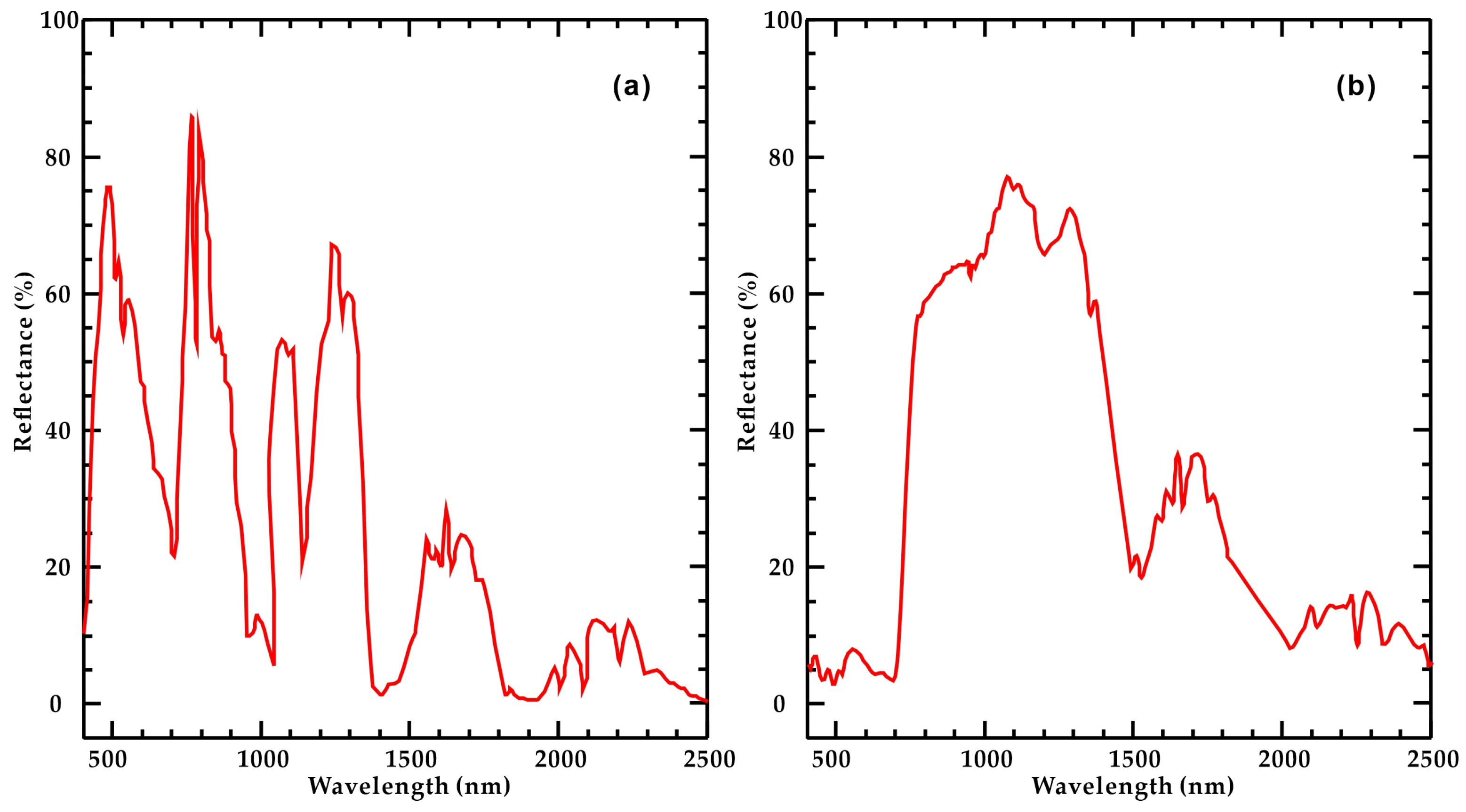
To evaluate the accuracy of atmospheric correction, spectral curves of typical ground-cover pixels in the image were selected for comparison before and after correction (Figure 5a,b). Before correction, the raw spectral curves exhibited overall high reflectance and a flat profile, lacking the characteristic absorption and reflection peaks expected for vegetation or rocks in the visible to near-infrared range (450–900 nm). This was primarily due to the superposition of atmospheric molecular scattering and water vapor absorption; no distinct water vapor absorption bands were observed in the short-wave infrared regions (1350–1450 nm and 1800–1950 nm), indicating that atmospheric effects masked the true spectral response of the land surface. After FLAASH atmospheric correction, the spectral curves of the same pixels regained the typical characteristics of natural surfaces: a reflection peak appeared near 550 nm, a chlorophyll absorption trough was observed near 680 nm, and reflectance increased rapidly in the near-infrared band (760–900 nm), consistent with the typical spectral profiles of vegetation or rocky surfaces; at the same time, distinct water vapor absorption troughs appear at 1400 nm and 1900 nm, coinciding with the locations of atmospheric water vapor absorption bands. A comparison of the images (Figure 6) shows that the pre-corrected image appears generally grayish with low contrast and blurred object boundaries; in the post-corrected image, colors are rendered naturally, tonal differences between areas of varying rock types and vegetation are significantly enhanced, and textural details are clearer. The restoration of the aforementioned spectral patterns, combined with the visual enhancement of the imagery, collectively demonstrates that atmospheric correction effectively removes the effects of atmospheric scattering and absorption. The resulting surface reflectance data exhibit high spectral fidelity and meet the accuracy requirements for the subsequent quantitative extraction of diagnostic absorption trough parameters.

Since the hyperspectral and panchromatic/multispectral cameras on board the ZY1-02E satellite are pushbroom imaging systems, differences in the sensitivity of the detection elements result in striping noise along the track direction, which can interfere with subsequent spectral feature extraction. Therefore, this paper employs a “global demosaicing” method to remove the striping noise, with the calculation formula as follows [40]:

$${\mathrm{X}}_{\mathrm{i}\mathrm{j}\mathrm{k}}^{\prime }={\mathsf{\alpha }}_{\mathrm{k}}{\mathrm{X}}_{\mathrm{i}\mathrm{j}\mathrm{k}}{+\mathsf{\beta }}_{\mathrm{k}}$$

(3)

$${\mathsf{\alpha }}_{\mathrm{k}}=\overline{{\mathrm{s}}_{\mathrm{k}}}/{\mathrm{s}}_{\mathrm{i}\mathrm{k}}$$

(4)

$${\mathsf{\beta }}_{\mathrm{k}}=\overline{{\mathrm{m}}_{\mathrm{k}}}-{\mathsf{\alpha }}_{\mathrm{i}\mathrm{k}}{\mathrm{m}}_{\mathrm{i}\mathrm{k}}$$

(5)

where ${\mathrm{X}}_{\mathrm{i}\mathrm{j}\mathrm{k}}^{\prime }$ is the grayscale value at row i and column j in band K of the corrected image, ${\mathrm{X}}_{\mathrm{i}\mathrm{j}\mathrm{k}}$ is the grayscale value at row i and column j in band K of the original image; ${\mathsf{\alpha }}_{\mathrm{k}}$ is the sensor gain value for band K, ${\mathsf{\beta }}_{\mathrm{k}}$ is the sensor offset value for band K, $\overline{{\mathrm{s}}_{\mathrm{k}}}$ is the standard deviation of band K in the reference image, ${\mathrm{s}}_{\mathrm{i}\mathrm{k}}$ is the standard deviation of row i in band K of the image to be processed, $\overline{{\mathrm{m}}_{\mathrm{k}}}$ is the mean value of band K in the reference image, and ${\mathrm{m}}_{\mathrm{i}\mathrm{k}}$ is the mean value of row i in the band K of the image to be processed.

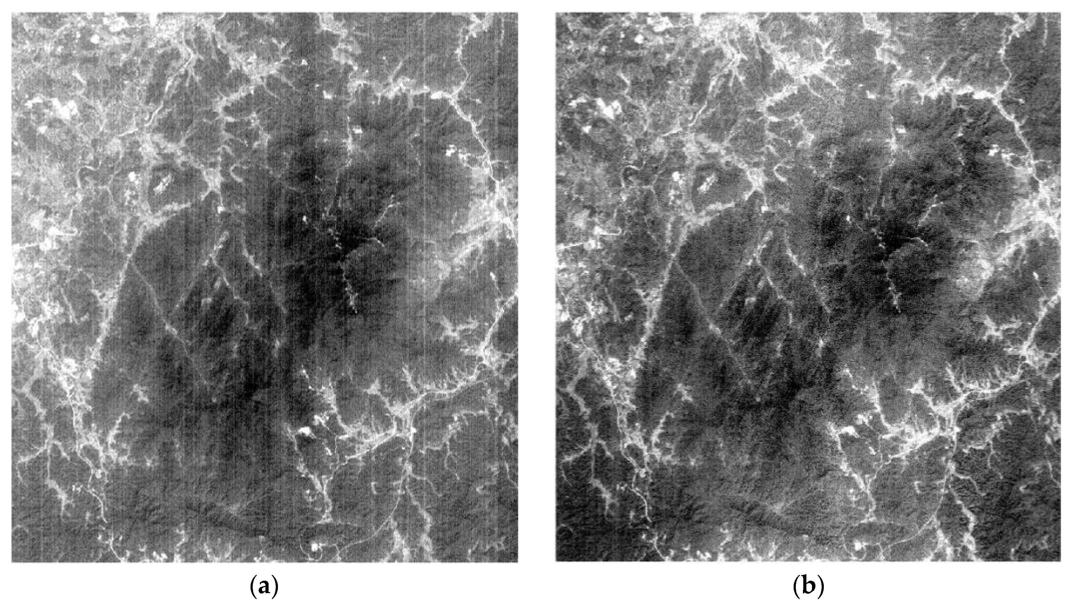
This article uses Python v3.9 programming to remove striped noise from images (see Appendix A for the complete code). The figure below shows a comparison of a 440 nm single-band image before and after stripe removal (Figure 7). After demosaicing, the quality of the hyperspectral image was significantly improved. In the pre-processing image (Figure 7a), numerous uneven light and dark stripes running vertically are visible, with multiple dense columns of brightness anomalies particularly evident in the left and central regions of the image; In the processed image (Figure 7b), these regular stripes have been largely eliminated, the brightness uniformity of the entire image has significantly improved, and the textures of land features previously obscured by the stripes have become much clearer. Furthermore, the processed image shows no obvious distortion in overall texture or brightness distribution, effectively preserving the spectral characteristics of the original land features.

To address the issues of geometric distortion and pixel displacement in hyperspectral imagery caused by satellite attitude, orbital altitude, and terrain undulations during the imaging process [41], this study employed the RPC (Rational Polynomial Coefficient) orthorectification workflow in ENVI software to perform orthorectification on the imagery. Following orthorectification, geometric distortions in the imagery were effectively eliminated, and the spatial matching accuracy between different spectral bands as well as between the imagery and the vector base map was significantly improved. Verification using several ground control points showed that the root mean square error of the orthorectified imagery was less than one pixel, indicating high geometric reliability. Following the aforementioned preprocessing workflow, the images possess unified geographic coordinates and reliable surface reflectance, laying a solid data foundation for subsequent pixel-level diagnostic absorption trough parameter extraction and alteration mineral mapping.

Finally, because the study area contains forested areas and shrubs, resulting in high vegetation cover, and given that the ZY1-02E imagery has a spatial resolution of 30 m, individual pixels are generally composed of a mixture of multiple components—such as vegetation, rock, clay alteration minerals, and Quaternary soils—resulting in a significant mixed-pixel effect. The absorption of chlorophyll and water by vegetation weakens the 2205 nm Al-OH absorption trough signal, leading to underestimates in the calculated depth and area of the absorption trough, and making it easy to overlook weak alteration zones. Therefore, the Normalized Difference Vegetation Index (NDVI) was used to create a mask to eliminate vegetation interference. The near-infrared band (860–1040 nm, corresponding to image band B56) and the red band (630–690 nm, corresponding to image band B32) were selected from the ZY1-02E hyperspectral imagery to construct an NDVI calculation model. combined with field sampling and statistical analysis of vegetation cover in the study area. A uniform threshold of NDVI = 0.3 was set for vegetation masking; pixels with NDVI > 0.3 (indicating dense vegetation) were masked out, retaining only pixels with NDVI ≤ 0.3—representing bare rock, bedrock with low vegetation cover, and thin soil layers—for subsequent quantitative extraction of absorption valley parameters. After masking, interference from the spectral components of vegetation in mixed pixels can be effectively eliminated, reducing the spectral overlap between the vegetation water absorption band and the clay Al-OH absorption valley. This ensures that quantitative parameters such as the depth, area, and symmetry of the 2205 nm absorption valley are determined solely by the spectral differences between hydrothermal clay alteration minerals and fresh host rock, thereby significantly enhancing the accuracy and quantitative reliability of subsequent alteration zoning results.

4. Spectral Characteristics of Major Rocks and Clay-Type Alteration Minerals in the Study Area and Their Implications for Ore Deposits

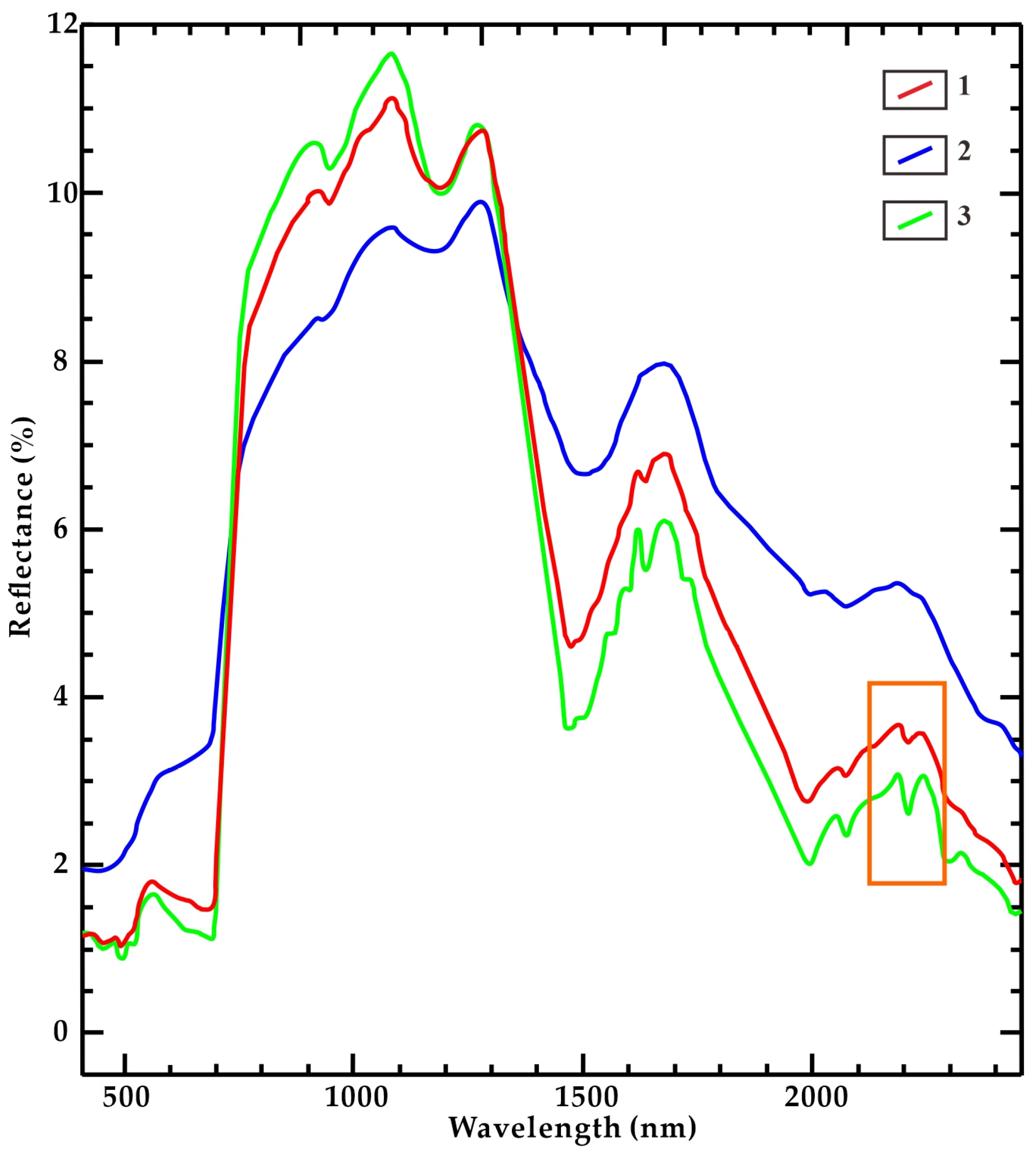
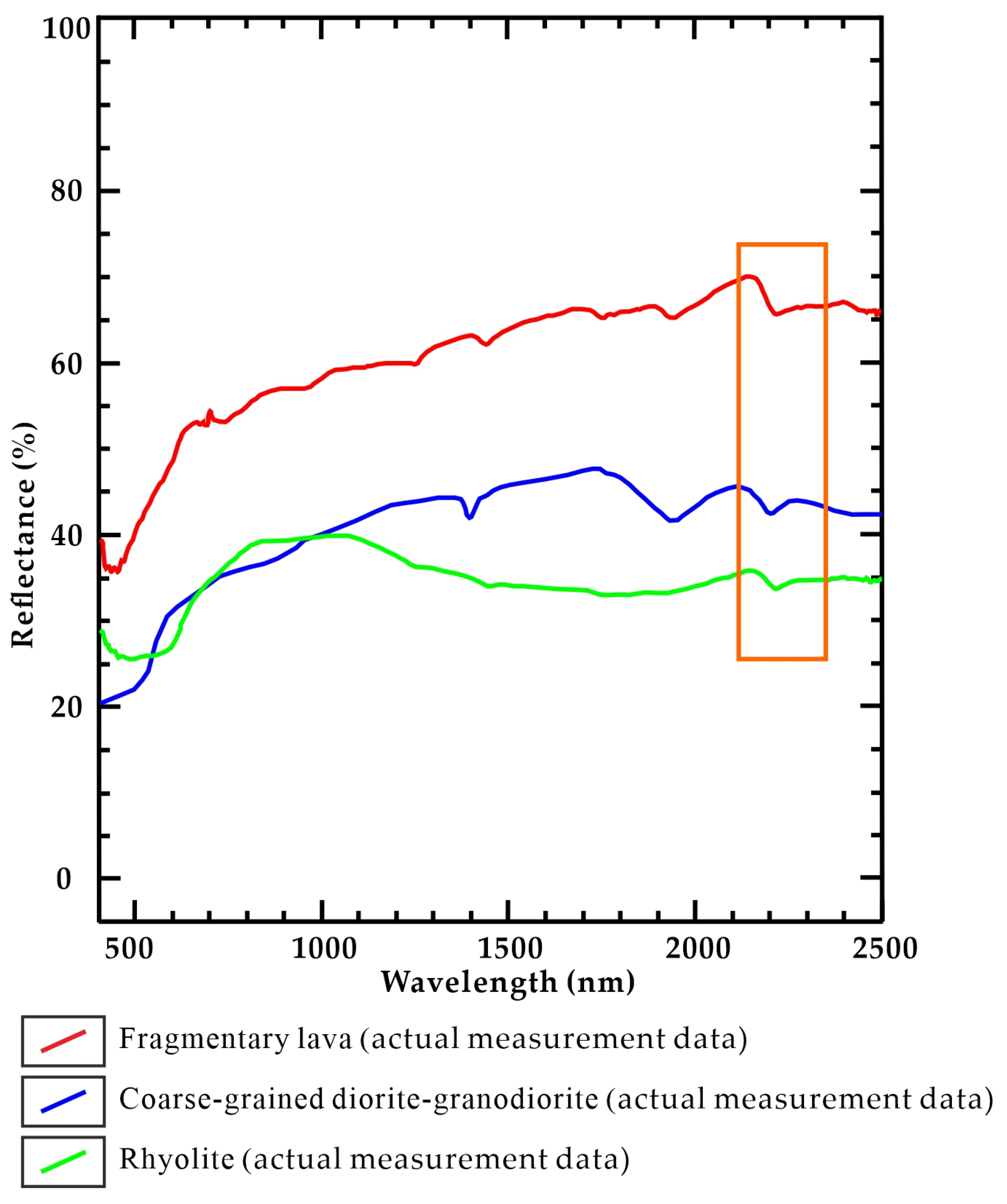
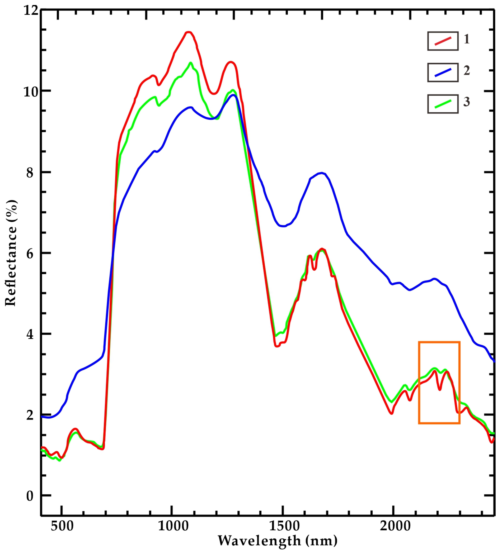
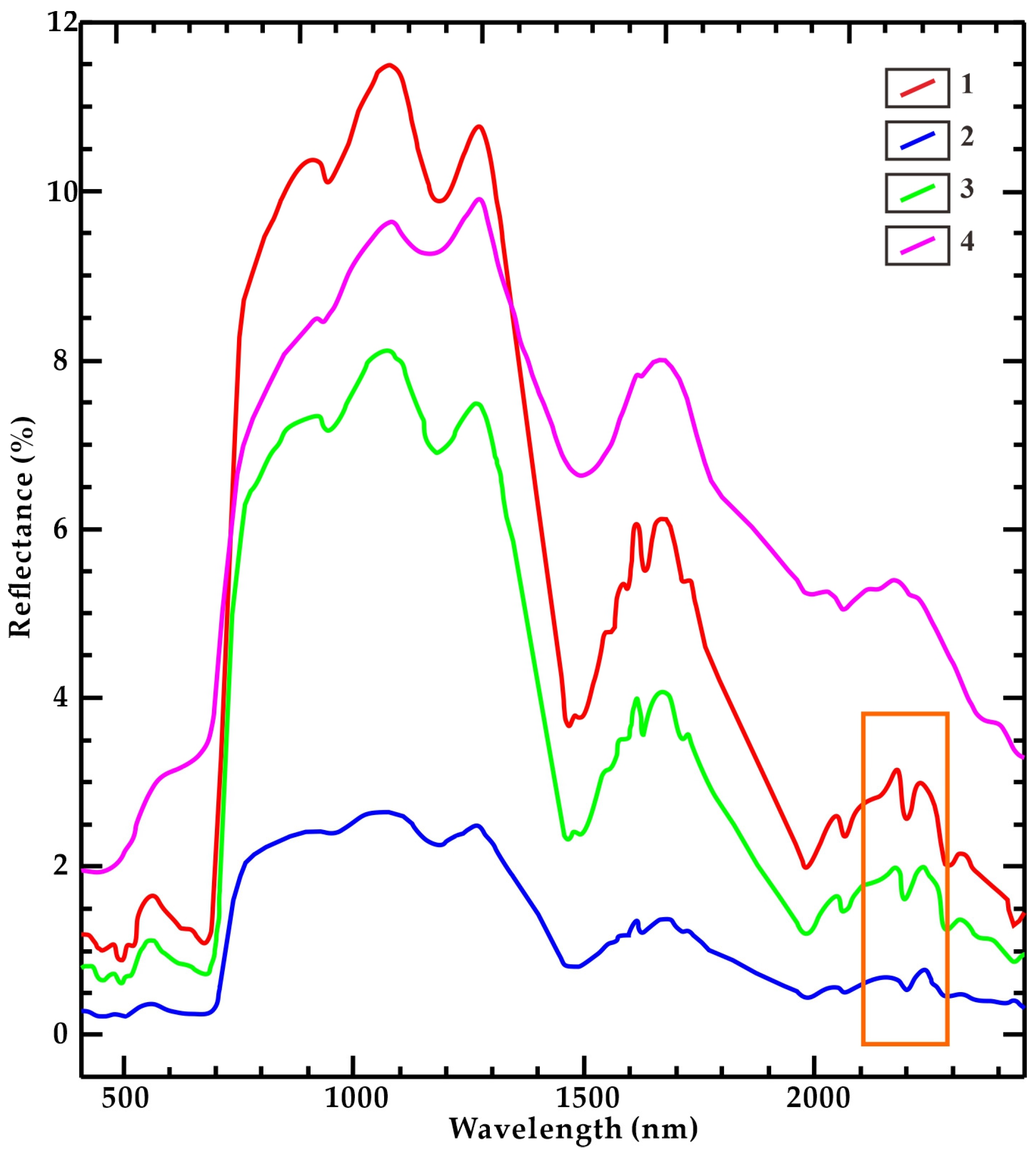
To obtain the reflectance spectral characteristics of the major rock types in the Xiangshan Uranium Deposit, this study used an SVC HR-768 portable spectrometer in a darkroom to measure the reflectance spectra of three major rock types: fresh, unaltered rhyodacite, fragmented porphyritic lava, and coarse-grained diorite porphyry. A 4° field-of-view lens was used for the measurements, with a quartz halogen tungsten lamp manufactured by THORLABS (Newton, NJ, USA) as the light source, and the spectral measurement range was 0.35–2.5 μm. Due to the instrument’s sensor limitations, the raw spectral data exhibited significant noise in the 0.9839–0.9996 μm and 1.8791–1.9237 μm bands; therefore, these segments were removed, and the remaining spectral curves were smoothed. Three spectral curves were measured for each sample, and the final reflectance spectral data were obtained by taking the average (Figure 8). The results show that, although no obvious alteration was observed with the naked eye, all three rock types still exhibited a faint absorption trough near 2205 nm. The origin of this weak absorption signal can be attributed to two main factors: First, due to residual hydrothermal activity during the late stages of magmatic crystallization, weakly acidic residual fluids permeated and altered feldspar phenocrysts, microfractures within the matrix, and grain boundaries—particularly along the cleavage fissures and grain edges of feldspar phenocrysts in fragmented feldspar lava—forming trace amounts of thin-film sericite. Although major aluminum-rich silicate minerals such as plagioclase and potassium feldspar do not exhibit diagnostic absorption features in the short-wave infrared band (0.35–2.5 μm), these scattered, secondary sericite- or clay-altered products are often distributed in thin-film form along cleavage planes, grain boundaries, and microfractures; the Al–OH groups they contain are sufficient to produce detectable, weak absorption signals. Second, biotite in the rock is prone to alteration after the magmatic stage or under epigene conditions, forming small amounts of muscovite; since muscovite contains Al–OH groups, it exhibits distinct spectral absorption features near 2.2 μm. Together, these two factors constitute the material basis for the weak absorption valley at 2205 nm. Such absorption valleys, caused by weak late-stage magmatic self-alteration or secondary mineral changes, are typically shallow and gentle, with low absorption depth values. In contrast, clay-rich alteration associated with hydrothermal activity, due to the large-scale enrichment of clay minerals such as illite and kaolinite, exhibits a deeper and broader characteristic absorption valley at 2205 nm. This significant difference in absorption depth provides a spectroscopic basis for distinguishing between unaltered and altered rock zones using absorption valley depth thresholds.

The clay alteration in the Xiangshan uranium deposit primarily consists of hydromica, chlorite, and sericite alteration, with hydromica being the predominant type. The hydromica is mainly composed of illite and illite–montmorillonite interlayered minerals [32]. These minerals are all layered silicate minerals or mineral assemblages that exhibit characteristic diagnostic absorption features in the visible-near-infrared spectral range (0.4–2.5 μm), making them important indicators for identification and quantitative inversion in hyperspectral remote sensing [42]. However, the aforementioned clay minerals do not exist in isolation; rather, they are direct products of the interaction between hydrothermal fluids and the host rock. Their types, crystallinity, and spatial zoning record information on the evolution of temperature, pH, and fluid composition during the hydrothermal alteration process. In the Xiangshan uranium deposit, uranium precipitation and enrichment primarily occur in the redox transition zone, and the hydrothermal fluid pathways indicated by clay alteration provide favorable physicochemical conditions for the migration and deposition of uranium complexes. Therefore, elucidating the spectral response characteristics of clay minerals is of significant indicative importance for understanding the uranium mineralization process.

Illite exhibits a distinct Al-OH absorption band near 2.2 μm. This absorption band is primarily caused by the vibration of aluminum-oxygen octahedra in the mineral lattice and serves as an important spectral indicator of clay alteration. The shape of the illite absorption band is typically sharp and symmetrical, reflecting its high crystallinity; this characteristic is often associated with high-temperature hydrothermal environments. Kaolinite also exhibits significant absorption near 1.4 μm and 2.2 μm. Its double-trough structure (particularly the strong absorption in the 2.16–2.21 μm range) is often used to distinguish it from minerals such as illite. The spectral characteristics of montmorillonite are similar to those of illite, with a distinct absorption trough near 2.2 μm. Montmorillonite frequently forms interlayered minerals with illite, and its spectrum exhibits a combination of the characteristics of both. The presence of interlayer water in montmorillonite results in a slightly broader absorption trough and reduced symmetry; this spectral difference serves as an effective criterion for distinguishing montmorillonite from illite. Chlorite exhibits an absorption band near 2.3 μm caused by Mg-OH, which differs from the absorption positions of illite and kaolinite; this is a key spectral feature for identifying magnesium-rich alteration.

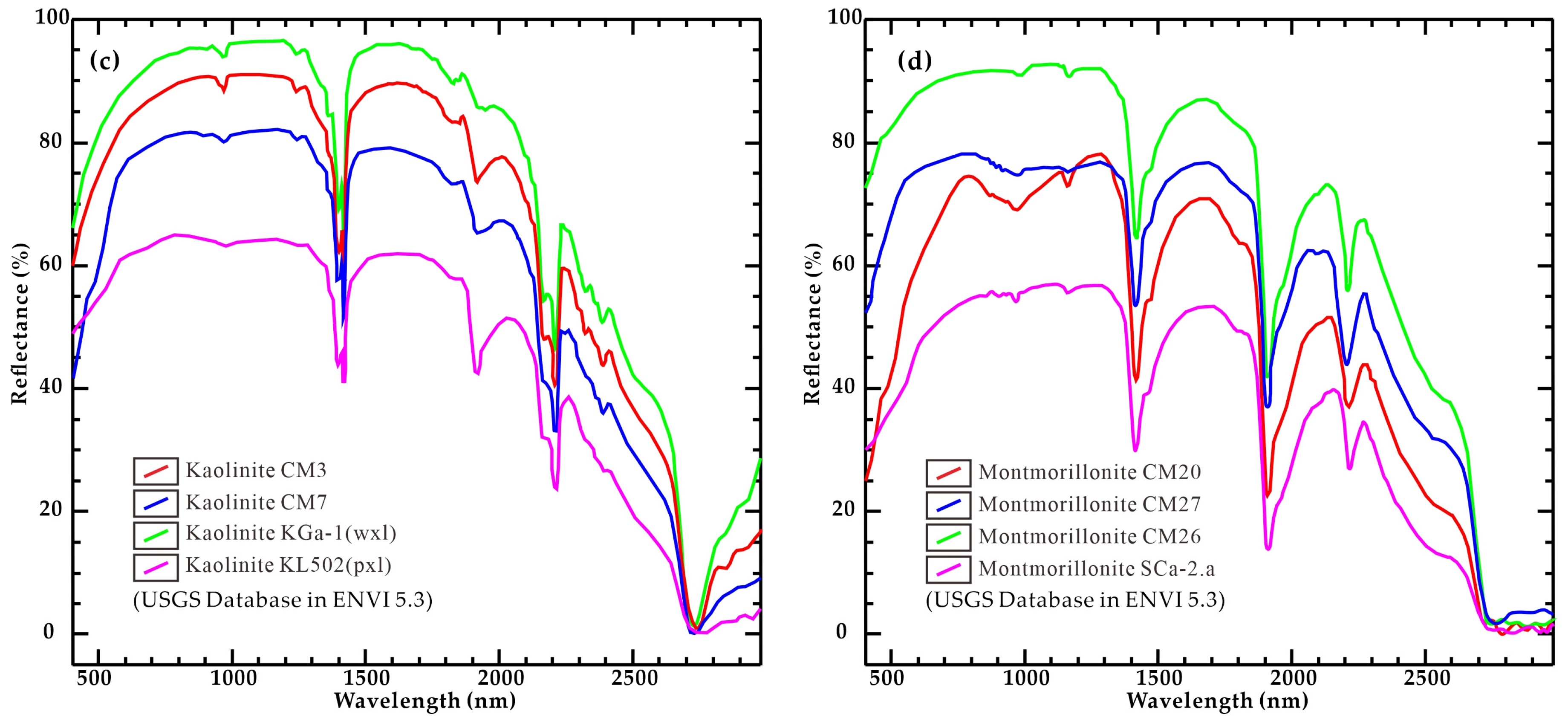
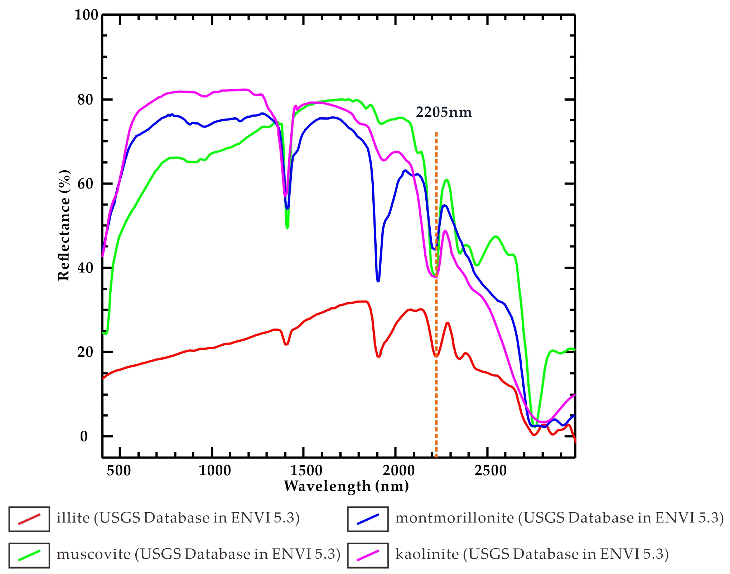
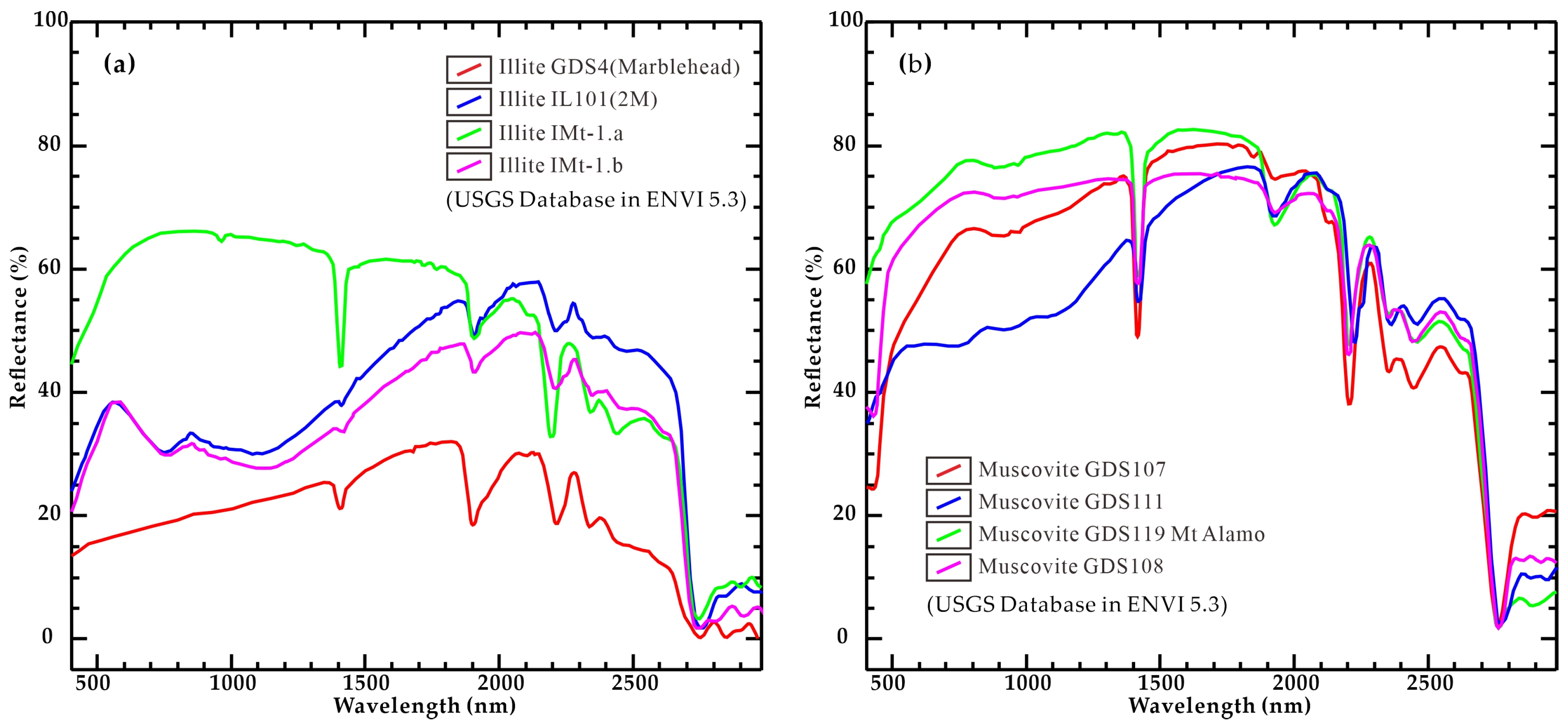
Based on the typical spectral curves in the “USGS Spectral Library” included in ENVI (Figure 9), the reflectance spectra of the aforementioned typical clay alteration minerals exhibit distinct absorption troughs. Kaolinite exhibits absorption troughs at 1413 nm, 1915 nm, 2165 nm, 2205 nm, and 2386 nm, with the absorption feature at 2205 nm being particularly pronounced; Illite exhibits water absorption bands at 1408 nm and 1905 nm, along with characteristic absorption troughs at 2205 nm, 2219 nm, and 2345 nm; montmorillonite’s absorption peaks primarily include water absorption bands at 1411 nm and 1905 nm, as well as a characteristic absorption trough at 2205 nm; The absorption features of muscovite are concentrated near 2205 nm, with water absorption bands at 1412 nm and 1925 nm, and secondary absorption bands at 2352 nm and 2442 nm. These spectral characteristics indicate that the region near 2205 nm is a concentrated response band for Al–OH bond vibrations. Systematic differences exist among various clay minerals in the shape, depth, and symmetry of absorption troughs in this band, providing a physical basis for quantitative mineral identification using hyperspectral data.

A comparison of the reflectance spectra of illite, dolomite, kaolinite and montmorillonite in the USGS spectral library reveals that, near 2205 nm, illite, muscovite, kaolinite and montmorillonite all exhibit distinct absorption troughs. Among these, the absorption troughs of illite and muscovite at this wavelength are relatively clear and symmetrical, reflecting the typical characteristics of Al-OH stretching vibrations in their structures; kaolinite also exhibits an absorption trough at this wavelength, though with slightly lower intensity; the absorption trough of montmorillonite is slightly broader, possibly due to the influence of interlayer water molecules. Overall, 2205 nm is a key wavelength band for identifying hydroxyl-related absorption in these silicate minerals. It can also be observed that the absorption troughs of illite, muscovite, kaolinite and montmorillonite at 2205 nm all exhibit a high left shoulder and a low right shoulder (Figure 10). Systematic variations in the geometric characteristics of the absorption troughs (such as depth, area, and asymmetry) essentially reflect differences in the order of Al-OH octahedra and the chemical environment within the mineral crystal structures. This provides measurable spectral parameters for the quantitative assessment of alteration intensity and hydrothermal activity stages.

The geological significance of these spectral differences lies in the fact that variations in the shape of absorption troughs can reflect environmental conditions—such as temperature and pH—during mineral formation. The crystallinity of illite is positively correlated with the sharpness of its 2205 nm absorption trough; highly crystalline illite typically forms in high-temperature hydrothermal environments, whereas low-crystallinity illite or illite–montmorillonite interlayered minerals are associated with low-temperature diagenesis or weak hydrothermal activity. In the Xiangshan uranium deposit, previous studies have shown that illite crystallinity decreases systematically from the mineralization center toward the periphery [5], and an increase in the proportion of montmorillonite within the illite–montmorillonite mixed-layer minerals indicates a decrease in alteration temperature and a weakening of hydrothermal activity. This spectral-genetic relationship provides a theoretical basis for inferring alteration environments using parameters such as the depth, area, and symmetry of the 2205 nm absorption trough.

Clay alteration is closely linked to uranium mineralization in terms of both spatial distribution and genesis. In the Xiangshan mineralized area, uranium is primarily hosted as pitchblende within sericite alteration zones; clay minerals are not only products of hydrothermal activity but also serve as important geochemical barriers for uranium precipitation and enrichment. Clay minerals can concentrate uranium through mechanisms such as adsorption, reduction, and ion exchange [32]; therefore, zones of intense clay alteration are often favorable sites for uranium mineralization. This study conducts a quantitative assessment based on parameters of the 2205 nm absorption trough, aiming to establish a spatial correlation between spectral response and mineralization intensity, thereby providing quantifiable remote sensing indicators for mineral exploration prediction.

The ZY1-02E satellite’s hyperspectral data offers the advantage of continuous, narrow-band coverage, with a spectral resolution of up to 10 nm in the short-wave infrared region, enabling the precise identification of diagnostic absorption features. To address the characteristic absorption trough of clay minerals near 2.20 μm, the ZY1-02E satellite has multiple contiguous bands in the 2.15–2.25 μm range, which can effectively extract parameters such as the location, depth, and area of the absorption trough, thereby enabling quantitative analysis of minerals. In addition, the bands set by the ZY1-02E satellite near 1.40 μm and 1.90 μm can be used to identify hydroxyl-containing minerals and help eliminate water vapor interference, thereby improving the reliability of alteration information extraction. Compared to wide-band multispectral data (such as ETM+ and ASTER), the ZY1-02E satellite’s hyperspectral characteristics significantly enhance the ability to identify subtle spectral differences in clay minerals, facilitating detailed mapping of clay alteration types and establishing quantitative relationships between spectral parameters and mineralization potential.

5. Quantitative Analysis of Diagnostic Absorption Feature

5.1. Quantitative Analysis Procedure of Diagnostic Absorption Feature

This paper focuses on analyzing the diagnostic absorption feature characteristics of clay minerals in the mineralized rock zones of the Xiangshan Uranium Mine. Specifically, this area includes the second member of the Ehuling Formation, the first member of the Ehuling Formation, the second member of the Daguding Formation, the first member of the Daguding Formation, the area covered by the Shazhou Unit, and the region within the outermost annular structure (Figure 1). Non-mineralized rock zones are excluded from this study.

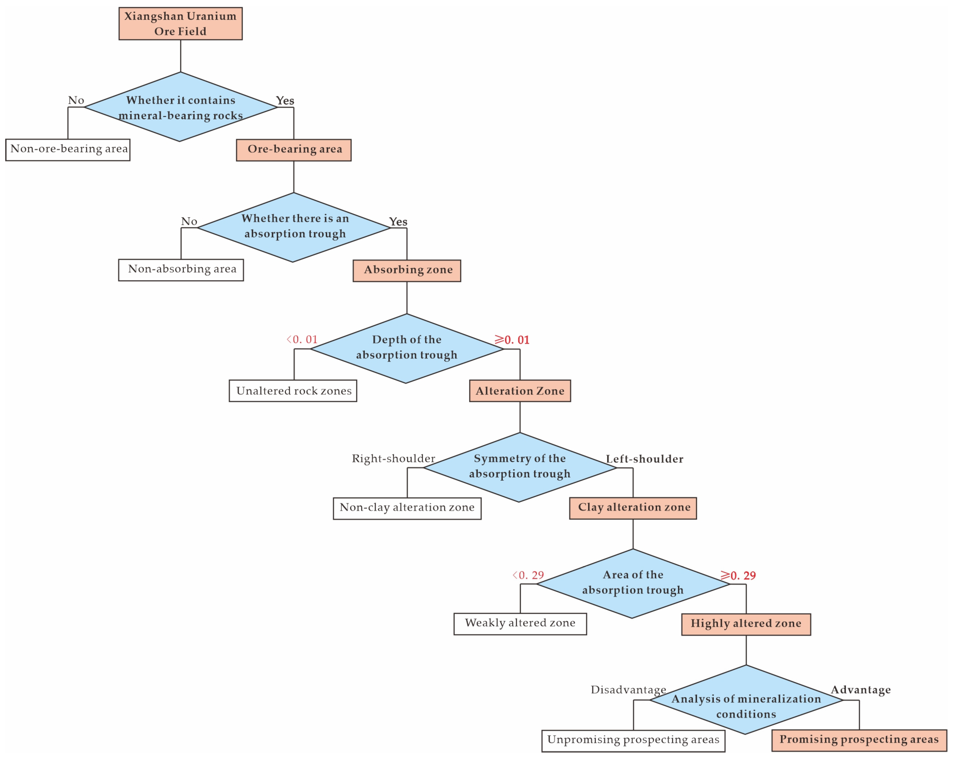
The quantitative analysis method for diagnostic absorption features proposed in this paper follows the main workflow shown in Figure 11: (1) identification and screening of effective absorption feature locations; (2) binary classification to determine the presence of absorption features in ore-bearing zones; (3) calculation of absorption trough depth; (4) using the globally averaged depth, areas with absorption depths below this value are classified as unaltered rock zones, while areas with absorption depths above this value are classified as altered mineral zones; (5) based on the symmetry of the absorption features, left-shoulder-type absorption troughs are defined as clay alteration zones; (6) based on the area of the left-shoulder-type absorption troughs, the clay alteration zones are further classified into weakly altered and strongly altered zones; and (7) on this basis, combined with qualitative analysis of favorable mineralization conditions, prospective exploration zones are delineated within the strongly altered zones.

5.2. Position of the Absorption Trough

When solar radiation is incident on mineral surfaces, differences in their internal chemical compositions and crystal structures cause them to selectively absorb and transmit incident light at specific wavelengths, thereby forming a series of indicative absorption features in the reflectance spectrum. These features give different minerals distinct “diagnostic” spectral responses, serving as a key basis for distinguishing between mineral types. The spectral characteristics of a mineral’s “diagnostic” absorption troughs can typically be quantitatively described using parameters such as absorption position, depth, area, width, and symmetry, as well as the spectral slope and spectral derivative. Among these, absorption position, absorption depth, absorption area, and absorption symmetry are key spectral indicators for identifying the content of clay-altered minerals [10].

In the short-wave infrared region, clay minerals typically exhibit distinct characteristic absorption bands near 2205 nm, 2260 nm, and 2350 nm, with the band at 2205 nm being the most pronounced. Therefore, this study selects the absorption trough at 2205 nm in the image spectrum as a diagnostic feature and performs a quantitative analysis of the depth, area, and symmetry of the absorption trough in the reflectance spectra of clay-altered zones within the Pingshan uranium deposit.

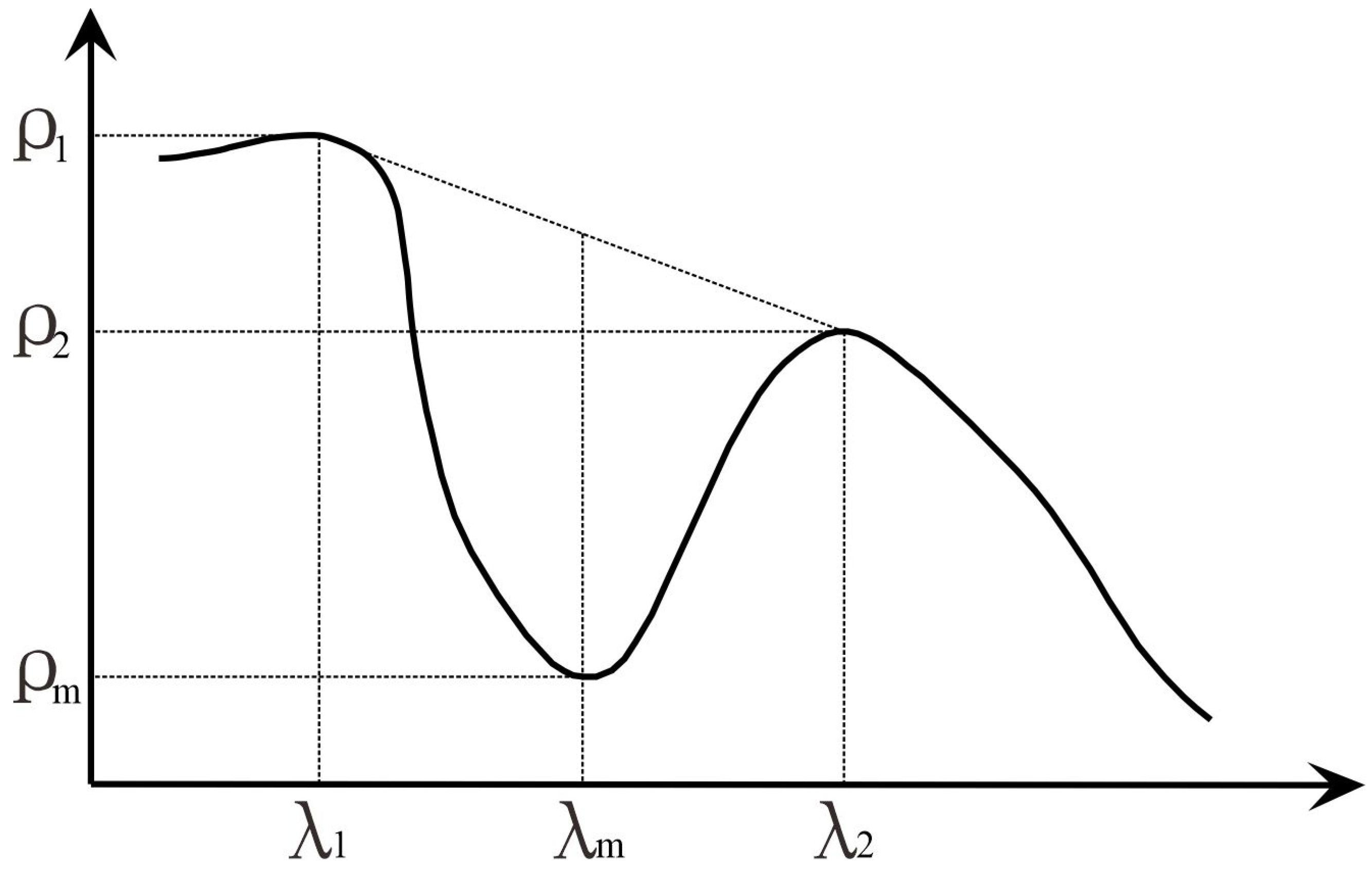
In hyperspectral imagery, the presence and specific location of an absorption trough in a pixel’s spectral curve are typically determined by calculating the first derivative of the pixel’s spectral curve. When an absorption trough exists in the spectral curve, its first derivative exhibits a regular sign change with wavelength. On the left side of the absorption trough, as wavelength increases, reflectance decreases, and the first derivative is negative. At the bottom of the absorption trough, the first derivative is zero or close to zero. To the right of the absorption trough, as wavelength increases, reflectance increases, and the first derivative becomes positive (Figure 12). Therefore, by analyzing the changes in the first derivative of the pixel spectral curve, absorption troughs can be effectively identified and localized.

Based on first-derivative features of hyperspectral imagery, this paper proposes an algorithm for identifying the 2205 nm absorption trough (see Appendix B for the complete code). The algorithm first calculates the minimum Euclidean distance between the input wavelength list and the target wavelength to accurately locate the band index where the target feature resides. Next, the algorithm analyzes the signs of the first derivatives on both sides of the target band on a pixel-by-pixel basis. If the derivative on the left is negative and the derivative on the right is positive, the location is preliminarily identified as a potential absorption trough. To further ensure detection reliability, the algorithm verifies whether the location satisfies the condition of a local minimum in reflectance, i.e., the reflectance in the target band must be lower than that of adjacent bands, thereby eliminating “false” absorption troughs. At the same time, by calculating the absolute values of the first-order derivatives of unaltered country rock, vegetation, and noise pixels, it can be seen that 99% of noise pixels have a first-order derivative absolute value < 0.001. Therefore, a derivative threshold of 0.001 is set to filter out instrument noise and spectral fluctuations caused by vegetation, while retaining faint signals from clay absorption troughs. This effectively balances detection sensitivity with noise suppression, thereby improving the ability to identify pixels with absorption characteristics. The selection of the derivative threshold is based on the signal-to-noise ratio of the sensor in the short-wave infrared band; 0.001 is the minimum effective response value for noise rejection. Values below 0.001 would introduce a large number of false absorption troughs, while values above 0.001 would result in the loss of weak alteration information. Ultimately, the algorithm outputs a binary map of the spatial distribution of absorption troughs (Figure 13).

Based on the binary image showing the presence of absorption valleys (Figure 13), the number of pixels in the non-absorption valley region was calculated to be 133,368, accounting for 20.87%; the number of pixels in the absorption valley region was 505,543, accounting for 79.13%. The average spectral curves for the absorption valley region, the non-absorption valley region, and the entire image were calculated separately (Figure 14). A comparison reveals that at 2205 nm, there is a marked difference between the spectral curves of the absorption valley region and the non-absorption valley region.

5.3. Depth of the Absorption Trough

The depth of the absorption valley is determined by the total relative content of clay minerals and serves as a direct quantitative indicator of the intensity of the rock–water reaction. As deep uranium-rich hydrothermal fluids migrate along tectonic fractures, they undergo metamorphic alteration with the surrounding rhyolite and basaltic lava host rocks, resulting in the massive precipitation of ions such as K⁺ and Al³⁺ and the formation of hydroxyl clay minerals such as illite and kaolinite; The more complete the hydrothermal–rock reaction, the higher the proportion of clay minerals in the rock, the stronger the selective absorption of short-wavelength radiation at 2205 nm, the higher the absorption trough depth value, and the greater the potential for uranium pre-enrichment. Therefore, the absorption trough depth can serve as a basic classification indicator of uranium mineralization potential. The depth of an absorption trough is defined as the vertical distance between the reflectance value at the trough floor and the line connecting the shoulder values on either side of the trough (Figure 12). The formula can be expressed as:

$$\mathrm{D}\mathrm{e}\mathrm{p}\mathrm{t}\mathrm{h}={\displaystyle \frac{{\mathsf{\rho }}_1+{\mathsf{\rho }}_2}{2}}-{\mathsf{\rho }}_{\mathrm{m}}$$

(6)

where Depth is the depth of the absorption trough, ${\mathsf{\rho }}_{\mathrm{m}}$ is the reflectance value at the bottom of the absorption trough (point ${\mathrm{\lambda }}_{\mathrm{m}}$), ${\mathsf{\rho }}_1$ is the reflectance value at the left shoulder of the absorption trough (point ${\mathrm{\lambda }}_1$), and ${\mathsf{\rho }}_2$ is the reflectance value at the right shoulder of the absorption trough (point ${\mathrm{\lambda }}_2$).

The results of the statistical analysis of the depth of the “2205 diagnostic absorption trough” are presented below (

Table 4. The absorption depth of the 2205 diagnostic absorption trough.

Minimum Value	Maximum Value	Average Absorption Depth	Standard Deviation
0.000001	0.409961	0.012547	0.004459

and

Table 5. Statistical Table of Absorption Depth and Frequency at the 2205 nm Absorption Dip.

Absorption Depth	Frequency	Cumulative%
0.000001	0.409961	1.25%
0.002	0.0203	2.03%
0.005	2.336789	9.56%
0.006	3.610988	16.13%
0.008	5.186325	25.07%
0.010	7.054504	36.60%
0.011	9.101111	50.22%
0.013	10.759245	64.81%
0.014	11.516784	78.43%
0.016	10.763001	89.03%
0.018	8.368458	95.52%
0.410	2.366527	100.00%

, Figure 15):

To distinguish the differences in spectral response at 2205 nm between altered minerals and unaltered rocks in the study area, it is necessary to clearly define the numerical boundary between their absorption depths. Although unaltered rocks such as porphyritic lava, rhyolite andesite, and monzogranite porphyry exhibit characteristic absorption valleys near 2205 nm, their absorption depths are generally shallow. This study also confirmed through darkroom spectral measurements that their absorption valleys at 2205 nm are relatively shallow (Figure 8), with absorption depth values significantly lower than the standard absorption depths of typical clay minerals such as illite and kaolinite in the USGS spectral library. Therefore, the statistical mean of the absorption depth at 2205 nm in the study area can naturally serve as a threshold for distinguishing between the two end members (the shallow-absorption zone of unaltered rocks and the deep-absorption zone of altered minerals). Accordingly, based on the binary image of absorption valley presence, this study uses the average absorption depth in the study area as a threshold: regions below this threshold are classified as unaltered rock zones, while those above it are classified as altered mineral zones (Figure 15). The classical adaptive thresholding method was employed to conform to the statistical differentiation patterns of mineral spectra, thereby extracting the distribution range of altered mineral zones based on absorption depth for subsequent analysis. Further statistical analysis was conducted on the data from the unaltered rock zones and altered mineral zones (

Table 6. Information Table for Unaltered Rock Zones and Altered Mineral Zones.

	Pixel Count	Percentage (%)	Minimum	Maximum	Weighted Average Absorption Depth
Unaltered rock zones	240,344	47.54	0.000001	0.012000	0.004101
Alteration zones	265,199	52.46	0.012001	0.409961	0.014431

), and the average spectral curves for these two types of zones were calculated separately (Figure 16). The results show that the absorption valley depth at 2205 nm in the average spectral curve of the altered mineral zones exhibits good consistency with standard spectral characteristics.

5.4. Symmetry of the Absorption Trough

Absorption troughs are typically not perfectly symmetrical in shape, and the height difference between their left and right shoulders serves as an important spectral feature for distinguishing land cover types. As shown in Figure 12, when the left shoulder is higher than the right shoulder, it is referred to as a “left-shoulder absorption trough”. Conversely, when the right shoulder is higher than the left shoulder, it is referred to as a “right-shoulder absorption trough”. Right-skewed absorption troughs are commonly observed in the spectral responses of iron-bearing minerals such as hematite or certain vegetation under stress conditions; this may be related to absorption edge effects or the asymmetry of electronic transitions. Left-skewed absorption troughs, on the other hand, are frequently seen in clay minerals or water-related absorption features, reflecting enhanced absorption or reduced scattering in the long-wavelength region. This asymmetry aids in the precise differentiation of various land cover types and serves as a crucial basis for feature extraction and model development in remote sensing [43].

In the alteration zone, calculate the difference between the left and right shoulders of the absorption valley at 2205 nm. The formula is as follows:

$$\mathsf{\theta }={\mathsf{\rho }}_1-{\mathsf{\rho }}_2$$

(7)

where $\mathsf{\theta }$ is the difference between the left and right shoulders of the absorption trough, ${\mathsf{\rho }}_1$ is the reflectance value at the left shoulder of the absorption trough (point ${\mathrm{\lambda }}_1$), and ${\mathsf{\rho }}_2$ is the reflectance value at the right shoulder of the absorption trough (point ${\mathrm{\lambda }}_2$).

Set the $\mathsf{\theta }$ threshold to 0.001. Absorption troughs where the difference between the left and right shoulders falls between −0.001 and 0.001 are classified as absorption troughs with similar left and right shoulders. If the difference is ≥ 0.001, the left shoulder is higher than the right shoulder, and the trough is classified as a left-skewed absorption trough. If the difference is ≤−0.001, the right shoulder is higher than the left shoulder, and the trough is classified as a right-skewed absorption trough. As demonstrated through comparative spectral analysis, most absorption troughs in the clay alteration standard curve are left-skewed (Figure 9 and Figure 10). Therefore, the distribution area of left-skewed absorption troughs is identified as the clay alteration zone, while the distribution areas of absorption troughs with close left and right shoulders and right-skewed absorption troughs are identified as non-clay alteration zones (Figure 17). The number of pixels in the non-right-skewed absorption trough region was calculated to be 93,721, accounting for 35.34%; the number of pixels in the absorption trough region was 171,478, accounting for 64.66%. The average spectral curves for the above three regions were calculated separately (Figure 18). The results show that the absorption valley feature at 2205 nm in the average spectral curve of the left-skewed absorption valley region is in very good agreement with the spectral characteristics of standard clay alteration minerals.

5.5. Area of the Absorption Trough

The area of the absorption trough comprehensively indicates the duration and spatial extent of hydrothermal fluid activity, while also reflecting the connectivity of tectonic fractures and fluid flux. When fluid seepage occurs only briefly through a single fracture, it results in only small, scattered areas of alteration; however, where NE- and NW-trending faults intersect to form ring-shaped structural zones, they create continuous fluid pathways. After the magmatic phase, hydrothermal fluids can circulate repeatedly over long periods, forming continuous, areal, or banded clay alteration zones along both sides of the fractures. Therefore, a large absorption valley area indicates a long fluid activity cycle and high flux, providing the spatial conditions for large-scale uranium enrichment and precipitation; conversely, pixels with small alteration areas are often located in isolated microfractures, where fluid supply is insufficient to support the formation of industrial-scale uranium mineralization. The area of the absorption trough is defined as the area enclosed by the spectral curve and the lines connecting the shoulder points on either side within the absorption feature wavelength range (Figure 12). This parameter reflects the overall intensity of the absorption feature. The calculation formula is as follows:

$$\mathrm{A}\mathrm{r}\mathrm{e}\mathrm{a}=\left[\left({\displaystyle \frac{{\mathsf{\rho }}_1+{\mathsf{\rho }}_2}{2}}\right)\times \mathrm{n}-\left({\mathsf{\rho }}_1+\cdots {\mathsf{\rho }}_{\mathrm{m}}+\cdots +{\mathsf{\rho }}_2\right)\right]\times \mathrm{\gamma }$$

(8)

$$\mathrm{\gamma }={\displaystyle \frac{{\mathrm{\gamma }}_1-{\mathrm{\gamma }}_2}{\mathrm{n}}}$$

(9)

where $\mathrm{A}\mathrm{r}\mathrm{e}\mathrm{a}$ is the area of the absorption trough, $\mathrm{\gamma }$ is the wavelength interval, $\mathrm{n}$ is the number of bands corresponding to the absorption trough, ${\mathsf{\rho }}_1$ is the reflectance value at the left shoulder of the absorption trough (point ${\mathrm{\lambda }}_1$), ${\mathsf{\rho }}_2$ is the reflectance value at the right shoulder of the absorption trough (point ${\mathrm{\lambda }}_2$), ${\mathsf{\rho }}_{\mathrm{m}}$ is the reflectance value at the trough of the absorption trough (point ${\mathrm{\lambda }}_{\mathrm{m}}$), $\mathrm{\gamma }$1 is the wavelength at the left shoulder, and $\mathrm{\gamma }$2 is the wavelength at the right shoulder.

A statistical analysis was performed on the diagnostic absorption trough areas at 2205 nm, and the results are shown in

Table 7. The absorption area of the 2205 diagnostic absorption trough.

Minimum Value	Maximum Value	Average Absorption Area	Standard Deviation
0.002252	0.478215	0.119866	0.085912

and

Table 8. Statistical Table of 2205 nm absorption trough area and frequency.

Absorption Area	Frequency	Cumulative%
0.002	0.0228	2.28%
0.013	0.0803	10.31%
0.032	0.0994	20.25%
0.055	0.0978	30.03%
0.081	0.1039	40.42%
0.107	0.0987	50.29%
0.135	0.0993	60.22%
0.165	0.0990	70.12%
0.200	0.1039	80.51%
0.243	0.0975	90.26%
0.292	0.0658	96.84%
0.478	0.0316	100.00%

:

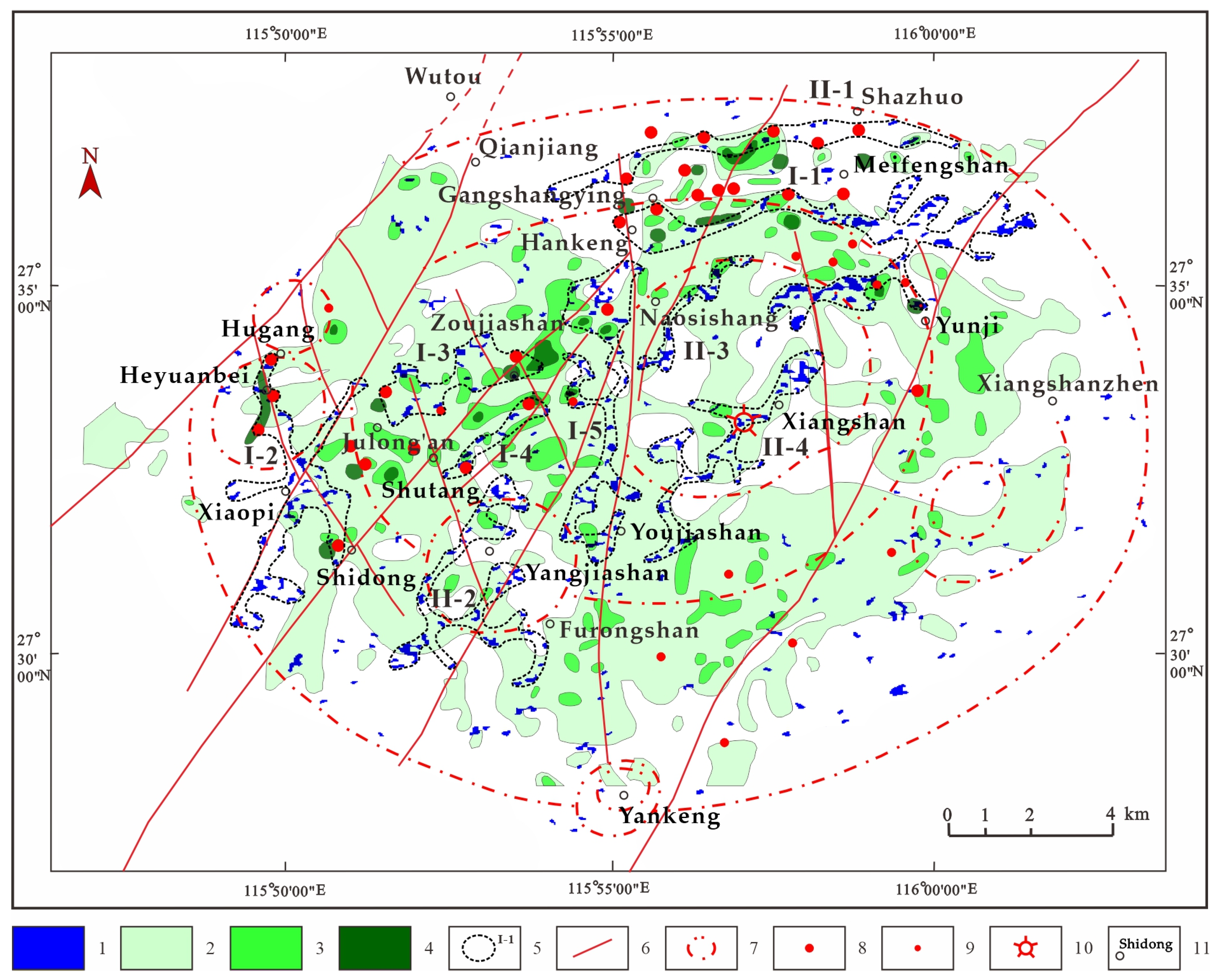
To suppress the interference of noise on alteration information, the images were first subjected to two rounds of 3 × 3 averaging filtering. Next, the thresholding method was used to delineate alteration anomaly zones. The threshold was set to “mean + N × standard deviation (σ),” where N was set to 2 to correspond to the 95% confidence interval under a normal distribution, ensuring the statistical significance of the anomalies while balancing the removal of background noise with the preservation of weak hydrothermal alteration. That is, data below “mean + 2 times the standard deviation” were removed to extract the alteration anomaly zones. To further visualize the distribution characteristics of alteration, the filtering tools in ENVI were used to remove isolated pixels and patches with excessively small areas; a pixel count threshold of 10 was set, and patches with fewer than 10 pixels were removed. To address the issues of voids and fragmentation in the processed results, the clustering tool was used to merge and fill neighboring pixels, ultimately producing a distribution map of clay alteration (Figure 19).

6. Analysis of the Distribution Characteristics of Clay Alteration and Prospecting Predictions

6.1. Analysis of the Distribution Characteristics of Clay Alteration

Based on the results of a combined analysis of the three parameters—absorption trough depth, area, and symmetry—clay alteration is primarily distributed in porphyritic lava and is also present in coarse-grained biotite granodiorite, though on a relatively limited scale (Figure 20). Overall, the distribution of alteration is clearly controlled by circular and linear structures, concentrated in areas of medium-to-high radioactivity, and generally coincides with the spatial distribution of known mineral deposits (locations). To quantitatively assess the relationship between alteration and radioactivity anomalies, this study performed a spatial overlay analysis of alteration intensity parameters and surface gamma-ray spectrometry data. The results show that the spatial overlap between high-alteration intensity zones and medium-to-high radioactivity anomaly zones exceeds 83%, and there is a clear overlap between areas with high gully depth values and areas with strong radioactive anomalies, indicating a clear spatial correlation between alteration anomalies and radioactive anomalies (Figure 21). This quantitative relationship provides empirical support for the validity of clay alteration as a uranium exploration indicator and suggests a close genesis-related connection between the two.

In terms of spatial distribution, the alteration zones primarily exhibit a combination of banded, ring-shaped, and nodular features. Using the line connecting Yankeng–Youjiashan–Xiangshan–Yunji as a boundary, alteration anomalies exhibit distinct spatial differentiation: on the northwestern side, alteration is densely distributed in large-scale continuous bands, with high intensity and clear zonation; absorption trough depths generally exceed 0.05, and area parameter values are high, indicating strong hydrothermal alteration centers. On the southeastern side, alteration is sporadic with poor continuity, and absorption trough parameter values are generally low. This spatial differentiation pattern is consistent with the asymmetric hydrothermal activity characteristics of the Xiangshan Volcanic Basin. Previous studies have suggested that tectonic and hydrothermal activity is more intense on the northwestern side; this study further validates this understanding from a quantitative spectroscopic perspective [23].

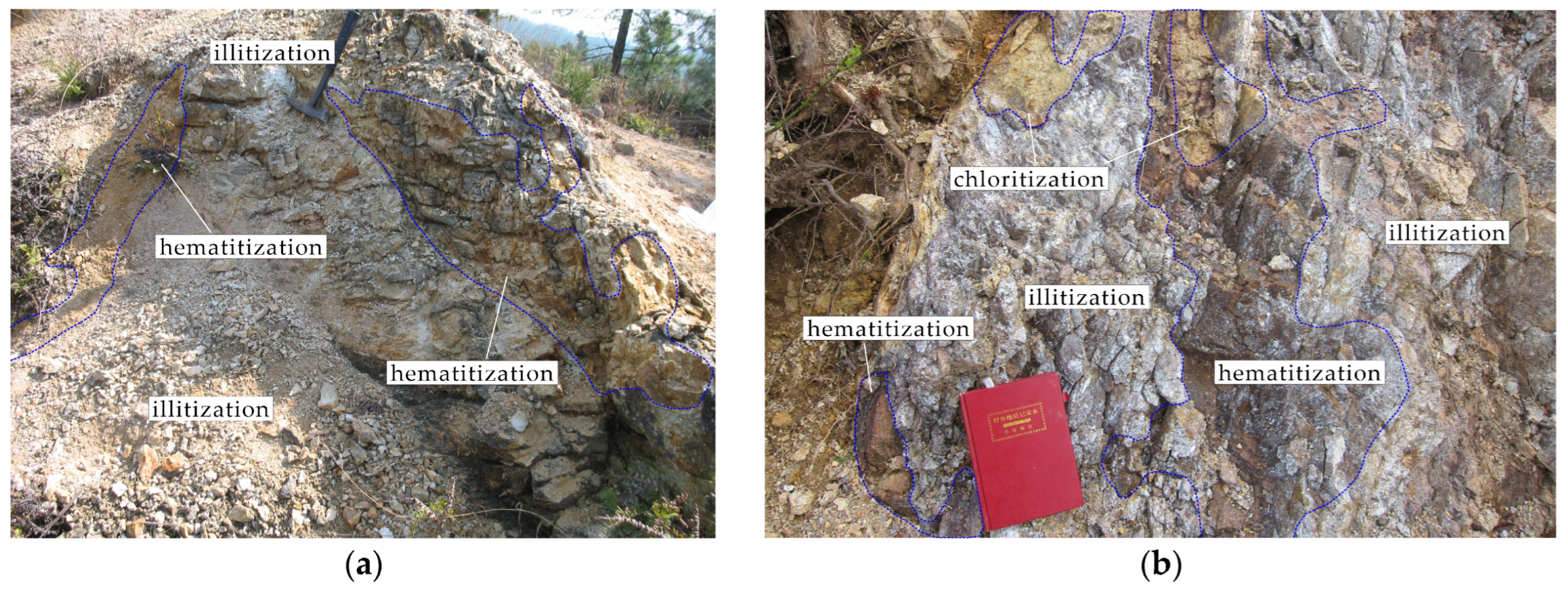
The areas of remote-sensing alteration anomalies generally coincide spatially with fault structures, ring-shaped structures, and known mineral deposits (locations), indicating that the distribution of alteration is clearly controlled by fault structures. As the primary transport pathways for hydrothermal fluids, faults play a key role in controlling the development of clay alteration. Areas of intense alteration show a high degree of overlap with fault lines; for example, in regions such as Heyuanbei (Figure 22a), Julong’an (Figure 22b), Xiaopi, and Yangjiashan, fault structures clearly traverse the centers of alteration zones, indicating that they provided pathways for hydrothermal activity and facilitated the formation of alteration minerals. The high permeability near fault zones facilitates fluid circulation and rock–water reactions, creating favorable ore-forming conditions and leading to the formation of extensive clay alteration zones along both sides of the faults. In particular, northeast-trending or northwest-trending faults dominate the spatial distribution of alteration, which is consistent with the regional tectonic setting of the Xiangshan uranium deposit. Deposits such as Heyuanbei, Shutang, Hankan, Julong’an, and Meifengshan are all located within areas of intense alteration anomalies, further corroborating the close spatial relationship between clay alteration and uranium mineralization.

6.2. Mineral Exploration Forecasting

By integrating multi-source information from the Xiangshan Uranium Field—including its fault structural framework, lithostratigraphic sequences, distribution of known deposits (points), surface radioactive anomalies, and parameters such as absorption trough depth, area, and symmetry extracted in this study—a total of 9 prospective exploration zones were delineated using a multi-parameter weighted spatial superposition method [45]. Level I prospective zones must simultaneously satisfy the following criteria: absorption trough depth > 0.02 (Table 5); the absorption area parameter falls within the top 30% percentile (the top 30% of pixels correspond to fault intersections and hydrothermal centers, and almost coincide with known large-scale deposits; the 70% low-value range consists only of sporadic, weak alteration), be located at fault intersections or areas where ring-shaped structures overlap, and be within a spatial distance of <1 km from known deposits (the hydrothermal alteration halo extends outward along faults to a maximum of approximately 1 km; beyond 1 km, the intensity of rock-water interactions decays rapidly, and there are no records of industrial-scale uranium mineralization) [2]. Level II prospective zones satisfy 2–3 of the above criteria, exhibiting larger-scale alteration but slightly lower parameter values. Based on these criteria, five first-level prospective zones (designated I-1 to I-5) and four second-level prospective zones (designated II-1 to II-4) were delineated (Figure 19 and Figure 20). The characteristics of each zone are as follows:

Zone I-1 (Hankeng–Meifengshan–Yunji Prospective Zone): The western part is primarily controlled by a ring-shaped structure. The uranium deposits in the Hankeng–Meifengshan area are also controlled by this structure. The distribution of alteration is a key indicator of uranium mineralization. The eastern part is controlled by the interaction of the ring-shaped structure and the northeast-trending Wuzhang–Yunji Fault Zone. Extensive clay alteration is exposed in this zone, showing high overlap with multiple known deposits (sites).

Zone I-2 (Heyuanbei–Xiaopi–Shidong Prospective Zone): Controlled jointly by the northwest-trending Heyuanbei–Shidong Fault and the northeast-trending Xiaopi–Qianjiang Fault. Alteration is generally distributed along the fault zones, with increased area and intensity at the intersection of the two fault systems. This intersection zone should be prioritized for future exploration.

Zone I-3 (Julong’an–Zoujiashan Prospective Zone): Controlled by both northeast-trending and northwest-trending faults. Alteration density increases significantly at fault intersections.

Zone I-4 (Shutang Prospective Zone): Controlled by a northeast-trending fault, it is located on the northwest side of the fault and shows good spatial correlation with the distribution of known deposits.

Zone I-5 (Hankeng–Youjiashan Prospective Zone): It generally trends north–south and is primarily controlled by the north–south Hankeng–Youjiashan Fault. At the intersection of the northeast-trending fault and this fault, the extent of alteration expands significantly.

Zone II-1 (Qianjiang–Shazhou Prospective Zone): Extending in a near-east–west direction, this zone is controlled by a ring-shaped structure and lies between two ring-shaped structural belts. It is situated within an area of dense mineralization, exhibiting a close relationship with uranium deposits. Alteration reflects surface information, while mineralization points represent the surface projections of deep ore bodies. There is a certain degree of deviation between the distribution of alteration and the locations of mineralization points.

Zone II-2 (Yangjiashan–Furongshan Prospective Zone): Controlled by a ring-shaped structure and possibly influenced by radial faults associated with this structure. Alteration exhibits a sheet-like distribution at the intersection of the radial faults and the ring-shaped structure, with a marked change in its orientation.

Zone II-3 (Naosishang Prospective Zone): It trends in a northeast direction and is clearly controlled by the northeast-trending Naosishang Fault.

Zone II-4 (Xiangshan Main Crater Prospective Zone): Traces a northeast-trending orientation, consistent with the direction of the main fault. Alteration is primarily distributed near the main crater and is closely related to the crater’s location.

Among these, in the Hankeng–Meifengshan–Yunji, Heyuanbei–Xiaopi–Shidong, Julong’an–Zoujiashan, Shutang, and Hankeng–Youjiashan prospecting zones, clay alteration occurs in sheet-like forms with intense alteration. These zones overlap significantly with the outer and middle rings of the main crater, exhibiting a distribution pattern where rings and lines intersect. They show the highest spatial correlation with known uranium deposits (sites) and should be prioritized as the primary prospecting zones for the next phase. The prospective exploration zones of Qianjiang–Shazhou, Yangjiashan–Furongshan, Naosishang, and the main crater of Xiangshan are distributed in an arc-like belt surrounding the outer edge of the high-value zone. From the area around Heyuanbei and Meifengshan to Youjiashan, they form a semi-enclosing transition zone. Their boundaries are jointly controlled by ring-shaped structures and northeast- and northwest-trending faults. The intensity of alteration increases in a clockwise direction from west to east and from north to south. Although the density of mineral deposits decreases, the scale of alteration remains substantial, making it likely to form secondary mineralization zones controlled by both tectonic and alteration factors. In contrast, the intensity of alteration anomalies in the eastern and southern parts of the mining area is generally below the background threshold, with absorption troughs mostly < 0.02. Alteration is weak, surface radioactivity is also low, and the exploration potential is limited.

7. Results and Discussion

7.1. Conclusions

(1)

This paper proposes a method for the quantitative identification of clay alteration based on the synergistic analysis of three parameters—the depth, area, and symmetry of the diagnostic absorption trough at 2205 nm—derived from ZY1-02E satellite hyperspectral data. This method effectively eliminates interference signals from unaltered rocks by applying an absorption depth threshold, distinguishes the spectral response differences between illite, kaolinite, and montmorillonite based on absorption symmetry, and delineates the extent of strongly altered zones using absorption area. This method focuses on quantitative evaluation based on absorption valley morphological parameters. Compared with traditional qualitative or semi-quantitative methods such as spectral angle mapping and principal component analysis, it has certain distinctive features in terms of alteration intensity grading and parameter quantification; however, its relative superiority still needs to be verified through direct comparative experiments using the same dataset.

(2)

This study quantitatively reveals the spatial distribution patterns of clay alteration in the Xiangshan uranium deposit. Delimited by the line connecting Yankeng, Youjiashan, Xiangshan, and Yunji, the alteration exhibits a distinct asymmetric distribution pattern characterized by “strong in the northwest and weak in the southeast,” with high-intensity alteration zones concentrated along fault intersections. Alteration bodies predominantly occur in a combination of banded, annular, and nodular forms, with this spatial structure being controlled by both regional fault structures and volcanic mechanisms. The significant positive correlation between the depth of the absorption trough and surface radioactivity intensity quantitatively confirms the validity of clay alteration as an indicator for uranium exploration.

(3)

Based on the weighted superposition of multi-source information—including multi-parameter data from absorption troughs, fault structures, and radioactive anomalies—a total of nine prospective mineral exploration zones have been delineated. Among these, there are 5 Class I prospective zones (Hankeng–Meifengshan–Yunji, Heyuanbei–Xiaopi–Shidong, Julong’an–Zoujiashan, Shutang, and Hankeng–Youjiashan), all of which exhibit high absorption trough parameter values, the superimposition of fault and ring-shaped structures, and spatial alignment with known ore deposits. There are 4 Class II prospective zones (Qianjiang–Shazhou, Yangjiashan–Furongshan, Naosishang, and Xiangshan Main Crater), which exhibit larger-scale alteration but slightly lower parameter values, distributed in an arc-like pattern around the periphery of the high-value zones. In areas distant from the aforementioned favorable zones and lacking obvious superimposed ring structures and faults, the Absorption trough parameters are generally below the threshold, and these areas are designated as zones with limited prospecting potential.

The multi-parameter analysis method based on diagnostic absorption troughs proposed in this paper does not rely on specific sensors or mineral end-member databases. As long as the target altered minerals exhibit distinct diagnostic absorption features at specific wavelengths, this method can be generalized for hyperspectral remote sensing detection in other hydrothermal mineralization zones. From the perspective of mineralization mechanisms, the spatial variation in absorption trough parameters reveals the pathways along which post-magmatic hydrothermal activity migrated along volcanoes and faults, triggering hydrothermal-rock interactions. Areas of intense alteration represent the locations where fluid migration and hydrothermal–rock reactions were most vigorous, and these areas are precisely the favorable sites for uranium precipitation and enrichment. Therefore, clay alteration is not only a mineralization indicator but also an external spectral reflection of the spatial structure of the hydrothermal mineralization system. Quantitative remote sensing methods established based on this understanding can provide a reliable scientific basis for deep exploration of the Xiangshan uranium deposit and similar volcanic-type uranium deposits.

7.2. Discussion

The analytical methods employed in this study have yielded preliminary results in the extraction of absorption trough parameters and the delineation of alteration anomalies; however, several limitations remain that require attention and refinement in future research.

(1)

Due to the high vegetation cover and complex topography of the study area, as well as the large scale of the study (hundreds of square kilometers) at the mineralized field level, coupled with constraints related to the project phase and the field sampling window, this study has not yet conducted systematic field validation. Consequently, there is a lack of supporting field-measured reflectance spectra and X-ray diffraction (XRD) sample data; therefore, this paper is currently unable to provide quantitative validation metrics, which is one of its primary limitations. In the next phase, we plan to conduct systematic field hyperspectral measurements and rock sample collection in the identified prospective exploration areas, followed by XRD analysis and field reflectance spectroscopy tests. This will allow for a quantitative assessment of the consistency between the clay alteration parameters extracted by remote sensing and the measured data, thereby verifying the reliability of this method. This will serve as an important direction for future research.

(2)

This study did not compare the method with commonly used host rock alteration extraction methods—such as spectral feature fitting, spectral angular mapping (SAM), and mixed-modulation matched filtering (MTMF)—using the same dataset; therefore, it is not possible to quantitatively demonstrate the advantages of this method in terms of detection accuracy and target detection efficiency. The core contribution of this method lies in incorporating morphological parameters of absorption valleys (depth, area, symmetry, etc.) into a quantitative evaluation system, providing a new approach to classifying alteration intensity; however, its performance metrics require validation through rigorous comparative experiments. Therefore, this paper does not claim that this method is absolutely superior to existing methods but rather regards it as a complementary approach to quantitative alteration analysis using remote sensing.

(3)

The description in this study regarding the spatial overlap rate between alteration anomalies and radioactive anomalies is based solely on rough statistics derived from raster overlay; no spatial correlation analysis or significance tests were conducted. This is primarily because the radioactive data used were aggregated results from previous studies, and the original pixel-level data were unavailable, making it difficult to conduct more detailed statistical analyses. Therefore, the aforementioned overlap rates should be regarded as qualitative references; future research will incorporate independently measured ground-based gamma-ray spectroscopy data to conduct rigorous statistical inferences.

In summary, this study provides a quantitative analysis method for clay alteration based on domestically developed hyperspectral satellites and has achieved preliminary, exploratory results at the Xiangshan Uranium Deposit. Future work will focus on strengthening field validation, multi-method comparisons, and rigorous statistical testing to advance this method from semi-quantitative exploration toward broader application.

References

1. Li, Z.; Chen, A.; Fang, X.; Ou, G.; Zhang, K.; Jiao, Y.; Xia, Y.; Chen, F.; Zhou, W.; Liu, Z.; et al. Metallogenic mechanism and superposition metallogenic model of the sandstone type uranium deposits in northeastern Ordos Basin. Miner. Depos. 2006, 25, 245–248. [Google Scholar] [CrossRef]
2. Guo, F.; Xie, C.; Jiang, Y. Geology of the Xiangshan-Lugang Area in Jiangxi and the Uranium and Polymetallic Mineralization Context; Geology Press: Beijing, China, 2017. [Google Scholar]
3. Zhang, S.; Yu, D.; Wu, R.; Zhang, L. Shoshonitic rock and uranium mineralizatin in Xiangshan uranium ore-field in Jiangxi. Geotecton. Metallog. 2005, 29, 105–114. [Google Scholar] [CrossRef]
4. Masoumeh, A.; Saeed, A.; Daniel, J. Application of ASTER data for exploration of porphyry copper deposits: A case study of Daraloo-Sarmeshk area, southern part of the Kerman copper belt, Iran. Ore Geol. Rev. 2015, 70, 290–304. [Google Scholar] [CrossRef] [Scilit]
5. Zhang, C.; Ye, F.; Wu, D.; Wang, J.; Guo, B. Characteristics recognition of imaging spectra for uranium mineralization altered mineral assemblage in Xiangshan. Uranium Geol. 2021, 37, 69–77. [Google Scholar]
6. Chen, Y.; Cheng, H.; Du, P.; Wei, J.; Lang, F.; Ding, K.; Suo, Z. A review of remote sensing detection and identificationmethods for underground coal fire areas. Remote Sens. Technol. Appl. 2025, 40, 816–834. [Google Scholar]
7. Wang, R.; Gan, F.; Yan, B.; Yang, S.; Wang, Q. Hyperspectral mineral mapping and its application. Remote Sens. Land Resour. 2010, 1, 1–3. [Google Scholar]
8. Cardoso-Fernandes, J.; Teodoro, A.C.; Lima, A. Remote sensing data in lithium (Li) exploration: A new approach for the detection of Li-bearing pegmatites. Int. J. Appl. Earth Obs. Geoinf. 2019, 76, 10–25. [Google Scholar] [CrossRef] [Scilit]
9. Dong, X.; Gan, F.; Li, N.; Yan, B.; Zhang, L.; Zhao, J.; Yu, J.; Liu, R.; Ma, Y. Fine mineral identification of GF-5 hyperspectral image. J. Remote Sens. 2020, 24, 454–464. [Google Scholar] [CrossRef] [Scilit]
10. Tong, Y.; Li, X.; Yang, J.; Wang, F.; Cao, S.; Wei, J. Identification of alteration minerals and linear structures andprediction of metallogenic favorable areabased on ZY-1-02D hyperspectral data. Geol. China 2025, 53, 60–76. [Google Scholar] [CrossRef]
11. Gan, F.; Wang, R.; Ma, A. Spectral identification tree (sit) for mineral extraction based on spectral characteristics of minerals. Earth Sci. Front. 2003, 10, 445–454. [Google Scholar]
12. Wang, Z.; Zhu, Z.; Wang, H.; Liu, Q. Applications of spectral angle mapping method in lithological identification. Natl. Remote Sens. Bull. 1999, 10, 61–62+64–66. [Google Scholar]
13. Tangestani, M.H.; Moore, F. Iron oxide and hydroxyl enhancement using the Crosta Method: A case study from the Zagros Belt, Fars Province, Iran. Int. J. Appl. Earth Obs. Geoinf. 2000, 2, 140–146. [Google Scholar] [CrossRef] [Scilit]
14. Carranza, E.J.; Hale, M. Mineral imaging with Landsat Thematic Mapper data for hydrothermal alteration mapping in heavily vegetated terrane. Int. J. Remote Sens. 2002, 23, 4827–4852. [Google Scholar] [CrossRef] [Scilit]
15. Zhang, Y.; Yao, F. Application study of multi-spectral ASTER data for determination of ETM remote sensing anomaly property: Taking Wulonggou region of eastern KunLun mountain range as example. Acta Petrol. Sin. 2009, 25, 963–970. [Google Scholar]
16. Ahmadfaraj, M.; Mirmohammadi, M.; Afzal, P. Application of fractal modeling and PCA method for hydrothermal alteration mapping in the Saveh area (Central Iran) based on ASTER multispectral data. Int. J. Min. Geo-Eng. 2016, 50, 37–48. [Google Scholar]
17. Frutuoso, R.; Lima, A.; Teodoro, A.C. Application of remote sensing data in gold exploration: Targeting hydrothermal alteration using Landsat 8 imagery in northern Portugal. Arab. J. Geosci. 2021, 14, 459. [Google Scholar] [CrossRef] [Scilit]
18. Sun, Y.; Nie, J.; Tian, F.; Qin, K.; Yang, G.; Wang, J. Alteration mineral mapping of the Xiangshan uranium core using HySpex imaging hyperspectral data and its geological significance. Geol. Explor. 2015, 51, 165–174. [Google Scholar] [CrossRef]
19. Yao, J.; Zhang, C.; Ye, F.; Xu, Q.; Tian, M. Hyperspectral alteration mineral feature and its geological significance of drill core in Zoujiashan uranium deposit of Xiangshan orefield. Uranium Geol. 2017, 33, 376–380. [Google Scholar] [CrossRef]
20. Wu, Z.; Hu, R.; Guo, F.; Liu, L.; Xie, C.; Jiang, Y.; Zhou, W. The extraction of alteration anomaly with remote sensing image of vegetation covered area in Xiangshan uranium field, Jiangxi province. Uranium Geol. 2013, 29, 112–118. [Google Scholar] [CrossRef]
21. Wu, Z.; Guo, F.; Li, H.; Xu, H.; Zhang, S.; Li, G.; Zhang, W.; Zhu, M. Application of principal component analysis in interpretation of alteration zone in the Xiangshan Volcanic Basin. Geotecton. Metallog. 2020, 44, 385–403. [Google Scholar] [CrossRef]
22. Li, Y.; Li, H.; Xu, F. Research progress of hyperspectral remote sensing monitoring in mine environmental contamination. Nonferrous Met. Sci. Eng. 2022, 13, 108–114. [Google Scholar] [CrossRef]
23. Guo, F.; Xie, C.; Deng, J. Methods and Practices of 3D Geological Surveys in Mining Areas: A Case Study of the Xiangshan Volcanic Basin in Jiangxi; Science Press: Beijing, China, 2017. [Google Scholar]
24. Chen, X.; Lu, J.; Liu, C.; Zhao, L.; Wang, D.; Li, H. Single-grain zircon U-Pb isotopic ages of the volcanic-intrusive complexes in Tonglu and Xiangshan areas. Acta Petrol. Sin. 1999, 15, 272–278. [Google Scholar]
25. Yang, Q.; Guo, F.; Zhou, W.; Qu, H. Geochronology and metallogenic model of the Xiangshan U-Pb-Zn deposits, southern Jiangxi, China. Earth Sci. Front. 2017, 24, 283–298. [Google Scholar] [CrossRef]
26. Shao, F.; Chen, X.; Xu, H.; Huang, H.; Tang, X.; Zou, M.; He, X.; Li, M. Metallogenic model of the Xiangshan uranium ore field, Jiangxi Province. J. Geomech. 2008, 14, 65–73. [Google Scholar]
27. Fan, H.; Wang, D.; Liu, C.; Zhao, L.; Shen, W.; Ling, H.; Duan, Y. Discovery of quenched enclaves in subvolcanic rocks in Xiangshan, Jiangxi Province and its genetic mechanism. Acta Geol. Sin. 2001, 75, 64–69. [Google Scholar]
28. Zeng, W.; Chen, R.; Xie, G.; Pang, W.; Wu, Z. Prospecting progress and prospective analysis of uranium deposit in Xiangshan ore field. J. East China Univ. Technol. 2019, 42, 101–107. [Google Scholar] [CrossRef]
29. Zhang, H.; Chen, Z.; Yang, N. Structural control over the ore in Hengjian-Gangshangying deposits in Xiangshan ore field, Jiangxi Province. J. Geomech. 2009, 15, 36–49. [Google Scholar]
30. Guo, F.; Li, Z.; Deng, T.; Qu, M.; Zhou, W.; Huang, Q.; Shang, P.; Zhang, C.; Yan, Z. Key factors controlling volcanic-related uranium mineralization in the Xiangshan Basin, Jiangxi Province, South China: A review. Ore Geol. Rev. 2020, 122, 103517. [Google Scholar] [CrossRef] [Scilit]
31. Huang, Z.; Li, X.; Cai, G. Alteration Zones and Alteration Types in Hydrothermal Uranium Deposits; Atomic Energy Press: Beijing, China, 1999. [Google Scholar]
32. Wen, Z.; Du, L.; Liu, Z. Relationship between hydromicatization and uranium mineralization in the Xiangshan orefield. Mineral. Depos. 2000, 19, 257–264. [Google Scholar]
33. Wu, Z.; Ye, F.; Guo, F.; Liu, W.; Li, H.; Yang, Y. A review on application of techniques of principle component analysis on extracting alteration information of remote sensing. J. Geo-Inf. Sci. 2018, 20, 1644–1656. [Google Scholar] [CrossRef]
34. Chen, B. ZY1-02E Satellite. Satell. Appl. 2022, 2, 70. [Google Scholar]
35. Yang, B.; Wang, M. On-orbit geometric calibration method of ZY-1 02C panchromatic camera. Natl. Remote Sens. Bull. 2013, 17, 1175–1190. [Google Scholar] [CrossRef] [Scilit]
36. Liu, Y.; Li, J.; Xiao, C.; Zhang, F.; Wang, S. Inland water chlorophyll-a retrieval based on ZY-1 02D satellite hyperspectral observations. Natl. Remote Sens. Bull. 2022, 26, 168–178. [Google Scholar] [CrossRef] [Scilit]
37. Wang, M.; Zhao, Q.; Xie, G. A super-resolution method for ZY-1 02E thermal infrared bidirectional sub-pixel shifted sampling mode. Natl. Remote Sens. Bull. 2025, 29, 1649–1658. [Google Scholar]
38. Tang, H.; Xie, J.; Dou, X.; Zhang, H.; Chen, W. On-Orbit vicarious radiometric calibration and validation of ZY1-02E thermal infrared sensor. Remote Sens. 2023, 15, 994. [Google Scholar] [CrossRef] [Scilit]
39. Dou, X.; Li, K.; Zhang, Q.; Ma, C.; Tang, H.; Liu, X.; Qian, Y.; Chen, J.; Li, J.; Li, Y.; et al. Estimation of Land Surface Temperature from Chinese ZY1-02E IRS Data. Remote Sens. 2024, 16, 383. [Google Scholar] [CrossRef] [Scilit]
40. Tan, B.; Li, Z.; Chen, E.; Pang, Y. Preprocessing of EO-1 Hyperion hyperspectral data. Remote Sens. Inf. 2005, 6, 36–41. [Google Scholar]
41. Chen, J.; Zeng, Q.; Jiao, J.; Ye, F.; Zhu, L. Spaceborne SAR image geometric rectification method without ground control points using orbit parameters modulation. Acta Geod. Cartogr. Sin. 2016, 45, 1434. [Google Scholar] [CrossRef]
42. Tong, Q. Spectral Characteristics of Typical Landforms in China and Their Analysis; Science Press: Beijing, China, 1990. [Google Scholar]
43. Yao, F.; Zhang, Y.; Yang, J.; Geng, X. Application of ASTER remote sensing data to extraction of alterration zoning information from Dexing porphyry copper deposit. Miner. Depos. 2012, 31, 881–890. [Google Scholar] [CrossRef]
44. Zhuo, H.; Yao, Y. Practical Application of Integrated Geophysical and Geochemical Remote Sensing Methods in Mineral Exploration in the Luobi Area of the Xiangshan Uranium Deposit. In Proceedings of the 2025 3rd National Mineral Exploration Conference, Nanchang, China, 17–19 September 2025; pp. 996–1001. [Google Scholar] [CrossRef]
45. Bian, Y.; Guo, Y.; Ju, X.; Jia, W.; Yang, Y. Research on metallogenic information detection by multi-source remote sensing spatial superposition technique. China Min. Mag. 2024, 33, 247–254. [Google Scholar] [CrossRef]
Figure 1. Geological Sketch Map of the Xiangshan Uranium Ore Field [23]: 1. quaternary residual and colluvial deposits; 2. Upper Cretaceous red beds; 3. granitic blocky porphyritic lava from the central facies of Stage II of the Lower Cretaceous Ehuling Formation; 4. transitional facies porphyritic lava from Stage II of the Lower Cretaceous Ehuling Formation; 5. Lower Cretaceous Ehuling Formation Stage II marginal-phase porphyritic basalt containing metamorphic clasts; 6. Lower Cretaceous Ehuling Formation Stage I sandstone and tuff; 7. Lower Cretaceous Daguding Formation Stage II rhyanite; 8. Lower Cretaceous Daguding Formation Stage I sandstone and tuff; 9. Lower Devonian Yunsan Formation sandstone; 10. Qingbaikou Series metamorphic rocks; 11. Early Cretaceous diorite; 12. Early Devonian diorite; 13. Early Devonian diorite; 14. angular unconformity boundary of the ring structure; 15. fault; 16. ring structure identified by remote sensing interpretation; 17. uranium deposits; 18. uranium occurrences; 19. crater; 20. place names.
Remotesensing 18 02550 g001
Figure 2. The synthesis column map of major lithology on Xiangshan mine field: 1. Early Cretaceous diorite; 2. granitic blocky porphyritic lava from the central facies of Stage II of the Lower Cretaceous Ehuling Formation; 3. transitional facies porphyritic lava from Stage II of the Lower Cretaceous Ehuling Formation; 4. Lower Cretaceous Ehuling Formation Stage II marginal-phase porphyritic basalt containing metamorphic clasts; 5. Lower Cretaceous Ehuling Formation Stage I sandstone and tuff; 6. Lower Cretaceous Daguding Formation Stage II rhyanite; 7. Lower Cretaceous Daguding Formation Stage I sandstone and tuff.
Remotesensing 18 02550 g002
Figure 3. Photograph of a section of rhyolite from the Daguding Group, Stage II.
Remotesensing 18 02550 g003
Figure 4. Photograph of the predominantly brecciated lava rocks of the Ehuling Formation, Stage II.
Remotesensing 18 02550 g004
Figure 5. Comparison of Spectral Curves for the Same Pixel Before and After Atmospheric Correction: (a) Spectral curves before atmospheric correction; (b) Spectral curve after atmospheric correction.
Remotesensing 18 02550 g005
Figure 6. Comparison of Images Before and After Atmospheric Correction: (a) image before atmospheric correction; (b) image after atmospheric correction.
Remotesensing 18 02550 g006
Figure 7. Comparison diagram before and after removing stripes: (a) the 440 nm image before processing; (b) the 440 nm image after processing.
Remotesensing 18 02550 g007
Figure 8. Spectral Curves of Major Rocks in the Xiangshan Region. (Within the area highlighted by the orange box, absorption troughs can be seen near 2205 nm).
Remotesensing 18 02550 g008
Figure 9. Spectral curve of clay alteration minerals.
Remotesensing 18 02550 g009
Figure 10. Spectral curves of illite, muscovite, kaolinite and montmorillonite: (a) spectral curve of illite; (b) spectral curve of muscovite; (c) spectral curve of kaolinite; (d) spectral curve of montmorillonite.
Remotesensing 18 02550 g010aRemotesensing 18 02550 g010b
Figure 11. Quantitative analysis flow chart of absorption feature.
Remotesensing 18 02550 g011
Figure 12. Schematic diagram of absorption trough.
Remotesensing 18 02550 g012
Figure 13. Binary map of the presence of the 2205 nm absorption trough: 1. non-absorbing zone; 2. absorbing zone; 3. fault; 4. ring structure; 5. uranium deposit; 6. uranium occurrence; 7. crater; 8. place name.
Remotesensing 18 02550 g013
Figure 14. The average spectral curve of absorption trough and non-absorption trough: 1. average spectral curve for the absorption trough region; 2. average spectral curve for the non-absorption trough region; 3. average spectral curve for the study area. (Within the area highlighted by the orange box, the characteristic absorption troughs near 2205 nm are visible).
Remotesensing 18 02550 g014
Figure 15. Map Showing the Distribution of Unaltered Rock Zones and Altered Mineral Zones: 1. unaltered rock zones; 2. alteration zones; 3. fault; 4. ring-shaped structure; 5. uranium deposit; 6. uranium occurrence; 7. crater; 8. place name.
Remotesensing 18 02550 g015
Figure 16. Average spectral curves for Unaltered Rock Zones and Altered Mineral Zones: 1. unaltered rock zones; 2. non-absorbing valley zones; 3. alteration zones. (Within the area highlighted by the orange box, the characteristic absorption troughs near 2205 nm are visible).
Remotesensing 18 02550 g016
Figure 17. The 2205 nm absorption trough symmetry classification diagram: 1. right-shoulder absorption trough; 2. left-shoulder absorption trough; 3. absorption trough with similar left and right shoulders; 4. fault; 5. ring-shaped structure; 6. uranium deposit; 7. uranium occurrence; 8. crater; 9. place name.
Remotesensing 18 02550 g017
Figure 18. The average spectral curves of absorption troughs with different symmetry: 1. average spectral curve for an absorption trough with a left-shoulder; 2. average spectral curve for an absorption trough with a right-shoulder; 3. average spectral curve for an absorption trough with peaks of similar width on both sides; 4. average spectral curve for an absorption trough with no peaks. (Within the area highlighted by the orange box, the characteristic absorption troughs near 2205 nm are visible).
Remotesensing 18 02550 g018
Figure 19. Clay alteration distribution map: 1. alteration anomaly; 2. fault; 3. ring-shaped structure; 4. uranium deposit; 5. uranium occurrence; 6. crater; 7. place name.
Remotesensing 18 02550 g019
Figure 20. Clay alteration distribution map: 1. quaternary residual and colluvial deposits; 2. Upper Cretaceous red beds; 3. granitic blocky porphyritic lava from the central facies of Stage II of the Lower Cretaceous Ehuling Formation; 4. transitional facies porphyritic lava from Stage II of the Lower Cretaceous Ehuling Formation; 5. Lower Cretaceous Ehuling Formation Stage II marginal-phase porphyritic basalt containing metamorphic clasts; 6. Lower Cretaceous Ehuling Formation Stage I sandstone and tuff; 7. Lower Cretaceous Daguding Formation Stage II rhyanite; 8. Lower Cretaceous Daguding Formation Stage I sandstone and tuff; 9. Lower Devonian Yunsan Formation sandstone; 10. Qingbaikou Series metamorphic rocks; 11. Early Cretaceous diorite; 12. Early Devonian diorite; 13. Early Devonian diorite; 14. angular unconformity boundary of the ring structure; 15. Fault; 16. ring structure identified by remote sensing interpretation; 17. uranium deposits; 18. uranium occurrences; 19. crater; 20. place names. 21. areas with clay alteration anomalies; 22. Prospecting target areas and their designations (I-1 through I-5 are primary prospecting zones; II-1 through II-4 are secondary prospecting zones).
Remotesensing 18 02550 g020
Figure 21. Clay alteration and radioactive superposition diagram (Radioactive data from [44]): 1. clay alteration anomaly zones; 2. medium-to-high radioactivity zones; 3. high radioactivity zones; 4. extremely high radioactivity zones (I-1 through I-5 are primary prospecting zones; II-1 through II-4 are secondary prospecting zones); 5. prospecting target zones and their designations; 6. faults; 7. ring-shaped structures; 8. uranium deposits; 9. uranium occurrences; 10. crater lakes; 11. place names.
Remotesensing 18 02550 g021
Figure 22. Field photographs of clay-altered rocks in a fault zone: (a) Heyuanbei Fault Zone; (b) Julong’an Fault Zone.
Remotesensing 18 02550 g022