Article

Impact of Clouds on Infrared and Microwave Sounding Retrieval and an Objective Correction Method for Numerical Weather Prediction


1
Department of Atmospheric Sciences, National Central University, Taoyuan 320317, Taiwan
2
Research Center for Environmental Changes, Academia Sinica, Taipei 115201, Taiwan
3
Central Weather Administration, Taipei 100006, Taiwan
4
National Science and Technology Center for Disaster Reduction, New Taipei 231007, Taiwan
*
Author to whom correspondence should be addressed.
Remote Sens. 2026, 18(15), 2549; https://doi.org/10.3390/rs18152549
Submission received: 14 April 2026 / Revised: 2 July 2026 / Accepted: 7 July 2026 / Published: 3 August 2026

Highlights

What are the main findings?
  • This study reveals that satellite-retrieved atmospheric temperature profiles exhibit significantly greater uncertainty below cloud layers and over land compared to over oceans or in clear-sky conditions.
  • Implementing an objective relative cloud-top pressure level (RCTL) criteria and correction method successfully reduced the retrieved water vapor mixing ratio dry bias.
What are the implications of the main findings?
  • Filtering out high-uncertainty temperature data and applying RCTL-dependent water vapor bias correction yields satellite profiles that are thermodynamically consistent with actual radiosonde observations.
  • Assimilating these objectively corrected soundings into regional weather models improves quantitative precipitation forecasts for challenging transition-season frontal systems while requiring fewer computational resources than direct radiance assimilation.

Abstract

Numerical weather simulations and forecasts are highly sensitive to environmental conditions. This is especially true in Taiwan, an ocean-surrounded island, during its transition season. Atmospheric temperature and moisture profiles retrieved from spaceborne sounders provide essential environmental information in regions lacking in situ observations. However, infrared sounders are sensitive to clouds and may induce uncertainties related to cloud properties. The present study analyzed 1 year of soundings from the National Oceanic and Atmospheric Administration’s Unique Combined Atmospheric Processing System (NUCAPS) to investigate the effects of clouds on the retrievals. The results indicated that the retrieved temperature profiles over land and under clouds had greater uncertainty than over oceans or in clear skies. In addition, the moisture profiles often exhibited a bias against cloud-top pressure. Therefore, this study proposed an objective quality control and bias correction method based on cloud effects. Excluding temperature observations affected by clouds and those over land reduced the root mean square difference from 3.3 K to 1.3 K. The relative cloud-top pressure level was used to conduct water vapor bias correction, which achieved effective correction for dry bias in the retrieved moisture profiles. After appropriate constraint criteria were applied, the bias-corrected profiles demonstrated a reduction in moisture bias from −4% to nearly 0%. That is, we assimilated sounding and radiance data into the regional Weather Research and Forecasting model and evaluated their effects, and we discovered that the retrieved profiles and direct observations positively contributed to the forecast of a spring frontal system. However, experiments using objective-bias-corrected sounding data improved skill scores in precipitation forecasts compared with using original sounding data or radiance data under a standard global operational baseline bias correction.

1. Introduction

The atmospheric state is a crucial and influential component of numerical weather simulations and modeling. Small differences in initial conditions can lead to diverse forecasting results. Therefore, utilizing observations to revise background state information may be beneficial in terms of improving routine weather forecasting and helping research focused on the underlying mechanisms of environmental states. In particular, satellite data, one of the nonconventional observation types, plays an important role when conventional data is sparse [1,2,3,4].
In a previous study conducted in Taiwan, Liu et al. [5] assimilated soundings from hyperspectral infrared and microwave spaceborne sensors at fine and coarse spatial resolutions, respectively. They reported that atmospheric temperature and moisture profiles retrieved from infrared or microwave sensors have a positive influence on numerical weather simulation and forecasting. In addition, they demonstrated the sensitivity of initial and boundary conditions during the transition season between spring and summer in the vicinity of Taiwan. During this transition season, large-scale flows do not substantially drive synoptic circulation, and small variations in the atmospheric thermodynamic state may lead to different patterns of evolution in the regional weather system. This indicates that a precise understanding of the initial field must be obtained to achieve accurate simulations or forecasts [6,7,8].
Notably, the atmospheric observations of advanced infrared and microwave spaceborne sounders are associated with low uncertainties, and they have enabled the retrieval of accurate temperature and moisture profiles [9,10,11,12]. These atmospheric profile data have been widely used in numerical weather prediction (NWP) and simulation models, with several studies contributing to the development of NWP models by assimilating radiance [13,14,15,16,17,18] and sounding [5,19,20] retrieval. Researchers have compared the relative contributions of radiance and sounding retrieval to NWP performance [21] and explored the outcomes of incorporating such data into models. Results have suggested that the equivalence of these approaches should satisfy two conditions. First, the radiance observation operator should approximate linearity in a region of the centered state space. Second, any prior information used to constrain retrieval should represent state variability. Whereas radiance is a fundamental quantity in observations, retrieved soundings are intuitive geophysical parameters. According to Zheng et al. [20], when the aforementioned conditions are met, fewer resources are required for data assimilation when soundings are used than when radiances are. During retrieval, a substantially larger number of channels is utilized compared to radiance assimilation especially for hyperspectral infrared sensors. The vertical structure of temperature and moisture may be better described in specific scenarios, such as during inversion in the atmospheric boundary layer.
The retrieved profile may be biased or uncertain relative to radiosonde observations (RAOBs) [22]. For example, overestimating surface emissivity may affect the forward calculation of radiance at the top of the atmosphere during numerical iteration [23,24,25]. This overestimation may cause the retrieved surface temperature, along with the temperature profile in the lowest atmosphere, to be lower than the reference. Moreover, the presence of clouds in the instrumental field of view may affect retrieval uncertainty because of the complexity of the radiative transfer process. Liu et al. [26] argued that greater uncertainty is associated with a higher field-of-view cloud fraction. Therefore, the quality of retrieved atmospheric temperature and moisture profiles must be quantified and analyzed in terms of both surface type and cloud properties. Another source of uncertainty in this context is the retrieval process depending on prior information during numerical iteration, which can dominate the retrieved moisture structure. For example, a single thick, moisture-rich layer in the atmosphere can produce radiances similar to those of several thin, moist layers, and this can complicate profile reconstruction [27]. Thus, surface microphysical characteristics, clouds, and optical properties remain difficult to measure using passive instruments such as microwave and infrared sounders.
When radiance data are directly assimilated, cloudy regions are often identified by noting differences between observations and background simulations [28]. Although this method can efficiently identify areas with a high probability of clouds, operators must be conservative in selecting relevant information. This often leads to the rejection of substantial observation data, which may include valuable information. Cloud-clearing retrieval can address this problem [29] and can be applied to obtain cloudy-area data for NWP. This method was adopted in National Aeronautics and Space Administration support products (SUPs) and continued in the National Oceanic and Atmospheric Administration (NOAA) Unique Combined Atmospheric Processing System sounding product (NSND). The NUCAPS retrieves atmospheric soundings from the observations of a Cross-track Infrared Sounder (CrIS) with an Advanced Technology Microwave Sounder (ATMS) or an Infrared Atmospheric Sounding Interferometer (IASI) with an Advanced Microwave Sounding Unit (AMSU) [30,31]. Several studies [20,28,29,30] have indicated that assimilating the retrieved data regarding the atmospheric thermodynamic state can improve NWP performance across different weather patterns without bias correction [20,32,33,34]. Notably, SUP and the NUCAPS can provide a unique dataset describing global atmospheric temperature and moisture profiles [35]. However, the retrieved soundings may contain biases related to temperature and moisture, and regional variability may lead to differences between sounding data and tropospheric temperature and moisture information inferred from radio occultation observations. According to the literature, SUPs contain both [19,31,32,33] cold and dry biases [19,35,36,37]. In consideration of this, a linear fit to the European Center’s reanalysis relative humidity field was used to address dry bias and improve forecasting for two typhoons. Singh et al. [38] evaluated the assimilation of SUP data for July 2010. Because they struggled to collect sufficient radiosondes near satellite-retrieved pixels, they calculated bias as the mean difference (MD) between retrievals and background at pressure levels and revised the profiles with this bias. However, in applying this method, they relied heavily on the background field, and the bias-adjusted initial condition consequently led to a poorer forecast [36]. In summary, retrieved profiles must be bias corrected.
In this study, we developed an objective quality control method based on the characteristics of NSND and bias in the cloudy field of regard (FOR) for water vapor profiles. Numerical experiments were conducted using the Weather Research and Forecasting (WRF) model and community grid point statistical interpolation. We evaluated the uncertainty of the NSND relative to various reanalysis fields before their assimilation into a numerical model (Section 2). We exclusively used the NSND because it has a long and stable history, which simplified the evaluation process and therefore enabled us to focus on bias removal. The method was based on the occurrence of clouds and their physical altitudes. In addition, our method was also applied in the study by Wang et al. [36], in which the corrected NUCAPS retrievals were assimilated into a cloud-resolving model for a Mei-Yu case. The results demonstrated improved model performance. Section 2 also presents the cold front case and numerical experimental design, Section 3 presents a result of the impact of these variables on the forecast obtained from the assimilation of objective NSND quality control and correction and presents a comparison of the proposed method with those involving conventional assimilation of radiances, and Section 5 concludes the paper.

2. Materials and Methods

The NUCAPS was developed to process CrIS and ATMS data aboard the SNPP and NOAA-20 satellites [39]. The products include temperature, moisture, and trace gas retrieval profiles. The cloud-top pressures and cloud fractions of two cloud layers were also included. In the NUCAPS algorithm, one ATMS footprint and the clearest of nine CrIS footprints were used to obtain a cloud-cleared infrared spectrum at the FOR. The product consisted of 100 pressure levels from the temperature and moisture profiles that ranged from 0.016 to 1100 hPa at a combined 45 km FOR at nadir. The clearest CrIS radiance produced a cold or dry bias in a few cloudy FORs, and bias correction was required. The NSND data in 5°S–45°N and 65°E–165°E from October 2019 to September 2020 was collected for the uncertainty analysis. Only NSND quality control flags of “accepted” were included in the uncertainty analysis (e.g Quality_Flag = 0). The recent data from June 2025 to May 2026 is shown in Appendix A. The SNPP and NOAA-20 passed this region at approximately 06Z and 18Z, at which times a few conventional observations were obtained. The European Center for Medium-Range Weather Forecasts reanalysis version 5 (ERA5) was used as a reference to identify the uncertainty of NSND. The NUCAPS obtained the same products using an IASI and AMSU, which were installed aboard Metop-A to Metop-C. Metop-A passed the region at approximately 00Z and 12Z, and the data it collected were retrieved for comparison with information from the ERA5 and the Integrated Global Radiosonde Archive (IGRA). The nearest NSND profile was matched with the ERA5 or IGRA, and the matched NSND was logarithmically interpolated to the pressure levels of the ERA5 or IGRA.

2.1. Temperature

The root mean square difference (RMSD) [5] and the square of the correlation coefficient (R2) were used to evaluate temperature performance:
R o o t   m e a n   s q u a r e   d i f f e r e n c e   ( R M S D ) = ( N S N D R E F . ) 2 N
where REF. refers to the reference data and N is the number of the sample size.
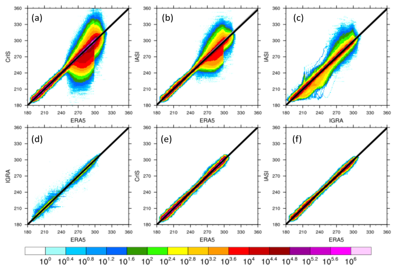
Most of the NSND retrieval temperatures exhibited a favorable relationship with the ERA5 (Figure 1); the data were distributed near the diagonal line. The temperature RMSD associated with CrIS retrieval was 3.3 K (R2 = 0.991), the temperature RMSD associated with IASI retrieval was 3.5 K (R2 = 0.990), and the RMSD calculated by the IASI and IGRA was 3.3 K (R2 = 0.988). The IASI presented similar results for the IGRA and ERA5, indicating that the ERA5 was sufficient to verify the performance of the NSND. A small portion of the data was sparse and deviated from the diagonal line, indicating major overestimation. In this area, the maximum temperature of the NSND was 407.2 K, whereas that of the ERA5 was 311.2 K. In addition, a discontinuous distribution was observed near the ERA5 at 300 K. This phenomenon indicated that further quality control was required for certain data to avoid the negative effects in data assimilation.
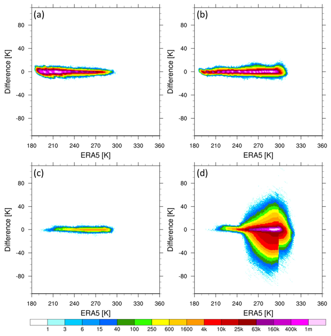
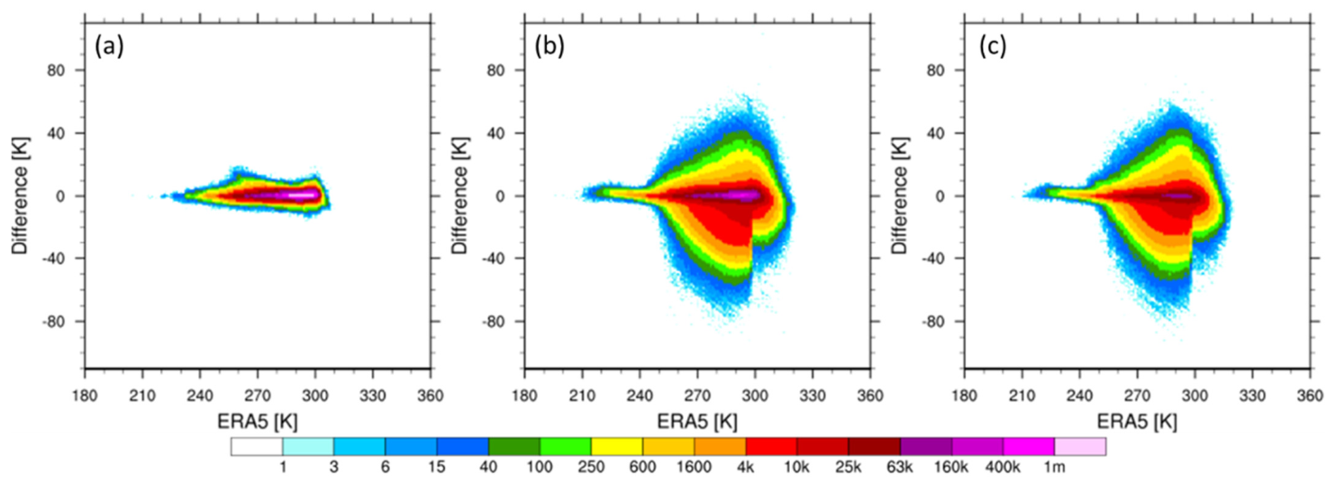
The NSND dataset provided information regarding two layers of cloud-top pressure. The cloud-top pressure in the first layer was lower than that in the second layer [40]. Analysis of the differences between the CrIS and ERA5 by cloud-top pressure category (Figure 2) revealed that 30.63% of the retrievals were from above the two layers of clouds, 38.93% were from between the two layers of clouds, and 30.38% were from below the two layers of clouds; cloud misplacement accounted for 0.06% of the total retrievals. The area between the two clouds presented good quality and a reasonable distribution, even though the cloud misplacement area also performed acceptably. These results confirm the effectiveness of cloud clearing in cloudy areas. Inconsistency occurred below the two-layer cloud area, where infrared retrievals were strongly affected by clouds. Because surface characteristics play a key role in retrieval, we categorized areas below the two clouds by land fraction (Figure 3). The data obtained for the ocean area were of high quality and were considered suitable for use in data assimilation. Discontinuity occurred mainly in the coastal and land areas, likely because of the land surface emissivity in the regression formulation. It indicates that the Masuda emissivity model [31], which was adopted in NUCAPS, performs well over the ocean. We further analyzed surface temperature, pressure, and topographic height, but we did not observe any notable patterns.
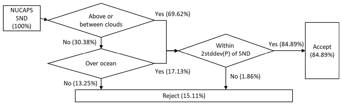
To ensure quality control for the NSND data, low-quality retrievals, including those affected by cloud contamination and complex surface emissions, were filtered out. As illustrated in the flowchart of quality control employed in this study (Figure 4), observations above clouds or between two cloud layers account for 69.62% of the total collected NSND. The remaining 30.38% of the total collected NSND is further evaluated based on whether it is over the ocean. If yes, this portion representing 17.13% of the total collected NSND is retained, while data over land is discarded. For cloud-affected profiles, retrieval accuracy is highly dependent on the underlying land fraction. Observations over the ocean were retained because marine emissions are generally stable. Observations located under clouds and over land were excluded from the analyses, with 13.25% of the total. This exclusion was considered necessary because land surface emission synthesis methods and oceanic models differ considerably. After this stage, the retained data account for 86.75% (69.62% + 17.13%) of the total collected NSND. The data that remained after the aforementioned screening process were subjected to a vertical consistency check to eliminate extreme values in the retrieved temperature profiles. A threshold was established for each vertical pressure layer that was within two standard deviations of the NSND mean. Any observation possessing a temperature value that exceeded this range in any vertical layer was identified as an outlier and subsequently removed. This statistical refinement led to an additional 1.86% of the data being rejected. Ultimately, 84.89% of the NSND data were accepted. The aforementioned process ensured that the dataset used for subsequent analysis and comparison was of high quality. After quality control, the RMSD for the CrIS and ERA5 was 1.3 K (R2 = 0.999), and the RMSD for the IASI and ERA5 was 1.5 K (R2 = 0.998).

2.2. Water Vapor Mixing Ratio

The relative difference (RD) [41] was used to determine the NSND water vapor mixing ratio, which substantially varies with pressure:
R e l a t i v e   d i f f e r e n c e   ( R D ) = ( N S N D R E F . R E F . ) × 100 %
where REF. refers to the reference data.
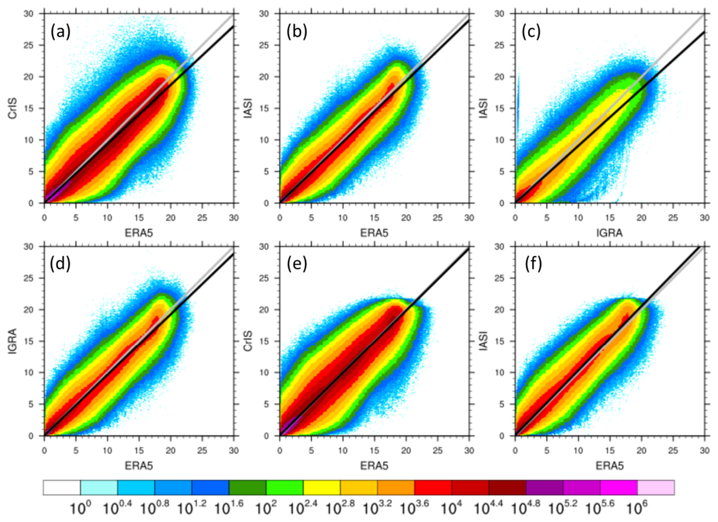
The moisture data this study retrieved from the NSND (expressed in terms of the water vapor mixing ratio) exhibited high performance against the ERA5 and IGRA (Figure 5). The mean RD (MRD) between the CrIS and ERA5 was −8.66% (R2 = 0.957), indicating little data exhibited wet bias. The maximum value was 80 g/kg, which is considered extreme. Additionally, the MRD between the IASI and ERA5 was −3.23%, with an R2 of 0.962. The difference between the IASI and IGRA was −10.95%, with an R2 of 0.905. Although there is no obvious dry bias in Figure 5a, previous studies [19,35,36,37] have indicated that dry bias commonly occurs in cloudy areas. In remote sensing, the level of retrieval is determined by optical depth and surface pressure. The optical depth represents the cumulative absorption and scattering of infrared or microwave radiation along the radiative path between the emission source and the satellite sensor. A larger optical depth indicates stronger radiation attenuation, which shifts the peak of the channel’s weighting function to a higher altitude, thereby limiting the sensor’s ability to see through dense low-level moisture or cloud layers. In the present study, the relative cloud-top pressure level (RCTL) was calculated using air pressure and the highest cloud-top pressure as vertical coordinates as follows:
R C T L = l n ( C T P h i g h e s t P )
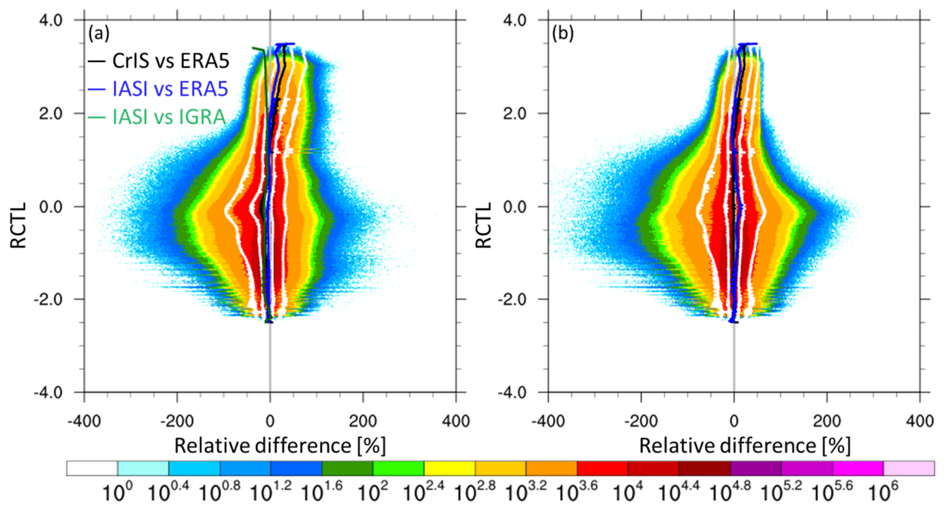
A positive RCTL indicates that the observation data are from above the cloud top, whereas a negative RCTL indicates that the observation data are from below the cloud top. A zero RCTL indicates that the observation data are from the cloud top. Figure 6a presents the RD and the vertical profile obtained by the RCTL. The RCTL was close to zero, and an obvious dry bias was observed. A wet bias was also observed in an area where the RCTL exceeded 1.5. Notably, the IASI exhibited wet bias when its data were compared with those of the ERA5 but not when compared with those of the IGRA. Ideally, satellites observe from space, so higher altitudes would be better than ERA5. Because of this, NSND indicating non-bias at higher altitudes is reasonable, and an RCTL greater than 1.5 should be reserved as the original value. However, the RCTL analysis indicated that nonbiased results were obtained at a value below −0.5. Because of this and because the data passed the NUCAPS’s quality control test, they can be used in this study. Nevertheless, when the level of bias was below the RCTL threshold of 1.5, the water vapor mixing ratio was processed by correcting retrieval bias as follows:
Q c = Q o Y ( R C T L ) × 100 % × Q o
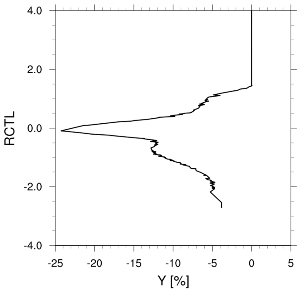
where the subscripts c and o represent the corrected and original values, respectively. This correction involved a synergistic approach, represented by the function Y (Figure 7), that targets the RCTL-dependent systematic MRD. This approach mitigated the distribution of biases through calculation of the MRD between the CrIS NSND and ERA5. This adjustment was strengthened through the use of a correction method designed to address the complex interplay between cloud structure and retrieval precision. Biases when the RCTL was larger than 1.5, where retrieval must have higher performance compared with the ERA5, were not corrected. To ensure data reliability, we filtered out outliers and retained 95% of the observations that were driest. This method utilizes the RCTL to identify and compensate for the dry bias often observed near the cloud top. This RCTL-based compensation enables nuanced refinement of moisture profiles that simple static corrections cannot achieve.
According to our results, the bias-corrected MRD of the CrIS was −0.74%, with an R2 of 0.958. The bias correction method with the same Y from the CrIS and ERA5 also applying to the IASI and which got the MRD was 4.31%, with an R2 of 0.959. After correction, the IASI bias shifted from dry to wet. This was because the correction was based on a full year of statistical data and only accounted for the level of clouds relative to that indicated by the ERA5 rather than the actual cloud morphology. Furthermore, because of the different satellite nadir times during the passage of the NOAA-20 and Metop-A, variations in weather conditions and the stage of convective development resulted in differences in cloud types. The cloud contamination patterns in infrared observations also differed. These results suggest that separate statistical analyses are still required for different sensors to achieve better performance. According to Chen et al. [31], bias patterns are generally inconsistent across different regions; therefore, the Y should be recalculated for individual areas. In the current context, Y represents the MRD of the CrIS and ERA5 at a specific RCTL (i.e., the black line in Figure 6a) and is presented as a lookup table. Biases exceeding 1.5 were not corrected [31].

2.3. Case and Experiment

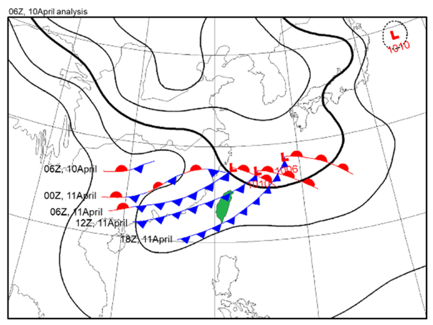
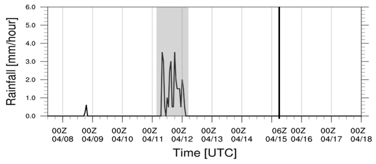
In Taiwan, obtaining forecasts during transition seasons is challenging because the environment near the island is characterized by mean moist static energy, similar to that in the vertical profile [42]. The present study tested its prediction model by considering a spring cold front that occurred in one of Taiwan’s transition seasons, that is, on 12 April 2020, to ensure quality control and review the effectiveness of the NSND’s bias correction. This front originated from the stationary front in the Sichuan Basin at 06Z on 10 April (Figure 8) and moved in the southeast direction, with a high-pressure front moving eastward. At 06Z on 11 April, its movement speed increased, and the system transformed into a cold front, which arrived in northern Taiwan at 12Z on 11 April. From 04Z on 11 April to 04Z on 12 April, the Taiwanese city of Taipei experienced hourly precipitation (Figure 9). The method proposed in this study was also used by Wang et al. [36], who assimilated the corrected NUCAPS retrievals into a cloud-resolving model for a Mei-Yu case and obtained improved results.
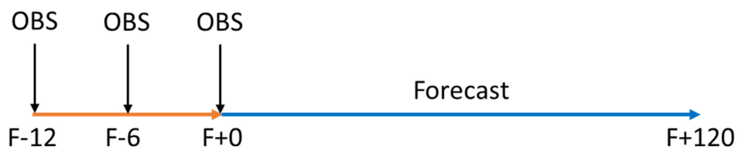
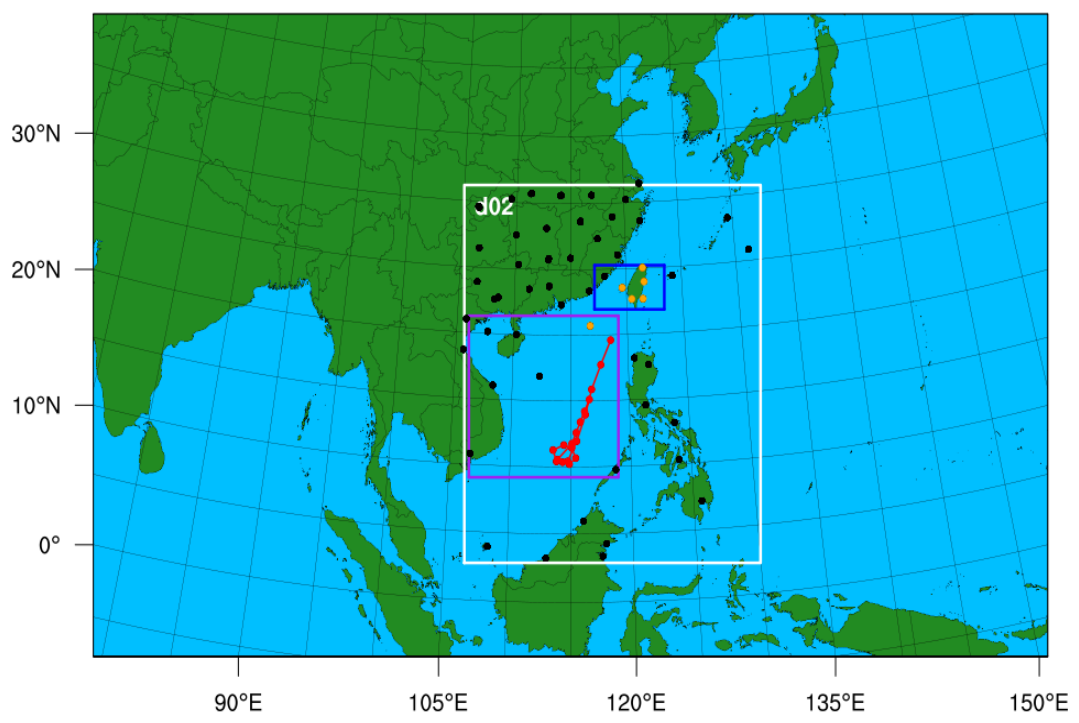
The advanced research version of the WRF model (version 4.2.1) was used as the regional NWP model. Data assimilation was performed using the Developmental Testbed Center’s Gridpoint Statistical Interpolation (GSI) system (version 3.5) with the three-dimensional Var method. Two domains (Figure 10) were configured with resolutions of 27 and 9 km around the South China Sea (SCS) with 55 vertical levels and a model top of 30 hPa. The new Tiedtke scheme was used as the cumulus scheme in all domains [43,44]. The Morrison two-moment scheme [45] and Yonsei University Scheme [46] were selected for microphysical and planetary boundary layer parameterization, respectively. Initial and boundary conditions were obtained from National Centers for Environmental Prediction (NCEP) final analysis data at a resolution of 0.25° × 0.25°. In the current study, a cold start was used in the first cycle of the spread experiments, with a cycling window of 12 h (Figure 11). Data were assimilated every 6 h, followed by 120 h of forecasting. The assimilated data were then tested (Table 1). Global telecommunications system (GTS) data were assimilated as a control experiment. Two experiments, namely SOR and SBC, were designed to investigate the influence of data bias correction on forecasts. The original NSND was used in the SOR experiment, and the quality-controlled NSND was used in the SBC experiment. The NSNDs obtained from the SNPP and Metop-A were used in both experiments. In addition, to compare the effects of assimilating sounding data versus those of assimilating radiance data, we conducted two experiments, namely RFS and ROP, and compared the results with those of the SOR experiment. In the RFS experiment, the operational radiance Binary Universal Form for data representation files were assimilated from 15 AMSU and 616 IASI channels aboard the Metop-A and from 22 ATMS and 399 CrIS channels aboard the SNPP, and the bias correction method and coefficients of the NCEP global data assimilation system were then applied. An additional ROP experiment was conducted in which only data from operational channels were assimilated. Subsequently, the Community Radiative Transfer Model was incorporated into the GSI system as a forward model, which was also adopted by NUCAPS [39]. A 45 km thinning mesh close to the NSND resolution at nadir was configured for the two radiance experiments. Seven forecasts were made as time-lag ensembles. All experiments involved data from the GTS, air force radiosondes, Central Weather Administration (CWA), and R/V Legend. The initial time range spanned from 12Z on 7 April 2020 to 12Z on 10 April 2020, per 12 h.
The R/V Legend had a mission over the SCS during the aforementioned timeframe, and it observed the atmospheric profiles in the region with radiosondes every 12 h (Figure 10). A radiosonde observed at 06Z on 15 April during the SNPP and NOAA-20 pass through the SCS. This provided a good opportunity to assess the impact of the data assimilation. This study also conducted an analysis filed for 06Z on 15 April, at which time the R/V Legend made a radiosonde observation to evaluate performance. Collocated NSNDs were observed under clear-sky conditions at the same time.

3. Results

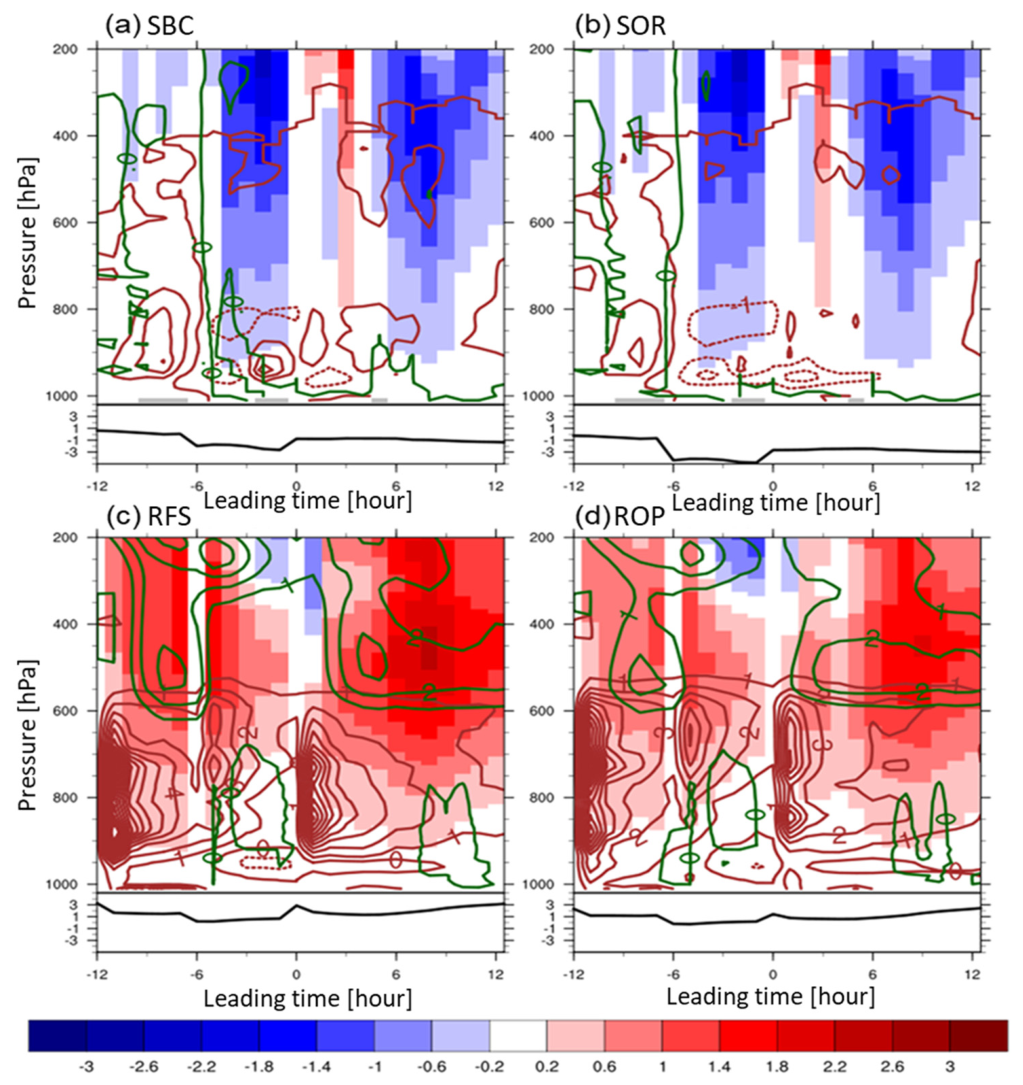
Because the SCS is the main source of water vapor of the fronts that affect Taiwan, this study analyzed changes to the SCS during cycling to evaluate the effectiveness of forecasting completed using the proposed model. In the SBC and SOR experiments (Figure 12a,b), small differences were observed in the first assimilation cycle. In the second assimilation cycle, a negative difference was observed in hydrometeors and vertical velocity. The first 6 h of forecasting indicated a higher vertical velocity at higher levels, but a noticeable reduction was observed at 6–12 h of forecasting. The total volume of precipitable water was consistently smaller in the forecasts than that indicated by the GTS. However, in the RFS and ROP experiments (Figure 12c,d), the forecasts indicated a higher water vapor content relative to that in the GTS observations. This higher water vapor content resulted in strong convection activity in the RFS and ROP experiments, which led to substantial liquid and solid water and a strong updraft. This phenomenon was also observed in the following cycles and forecasts.
All available radiosondes, including those obtained from the GTS, CWA, and R/V Legend, were used to assess the temperature, as MD [5] and RMSD, and the water vapor mixing ratio, as MRD and mean absolute RD (MARD) [41]:
M e a n   d i f f e r e n c e   ( M D ) = ( E X P . R A O B ) N
M e a n   a b s o l u t e   r e l a t i v e   d i f f e r e n c e   ( M A R D ) = | E X P . R A O B R A O B | N
where EXP. refers to the experiment data and N is the number of the sample size.
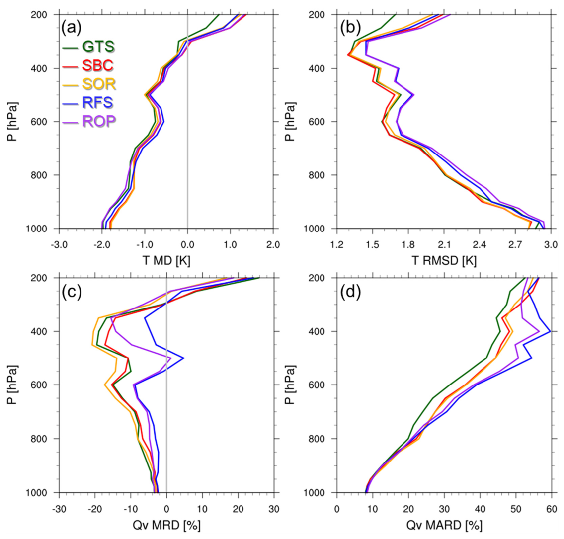
As presented in Figure 13, the GTS had an MD of 2 K from radiosondes at 1000 hPa. When the pressure decreased, this MD decreased to 0.8 K. Specifically, when the pressure decreased from 1000 to 350 hPa, the RMSD of the GTS decreased from 2.85 to 1.3 K (Figure 13b). Between 1000 and 500 hPa in Figure 13a, the MDs in the SBC and SOR experiments were similar and were smaller than those of the GTS. Below 850 hPa in Figure 13b, the RMSDs became smaller than those of the GTS, but they were nearly equal between 850 and 350 hPa. At high levels, the RMSD of the SBC experiment was slightly lower than that of the SOR experiment (Figure 13b). At 700 to 500 hPa in Figure 13a, the RFS experiment had the highest MD (close to 0) and the highest RMSD. At low levels, the ROP experiment had the lowest MD and the highest RMSD. Notably, the highest RMSDs of the RFS and ROP experiments were not suitable for forecasting.
The MRD and MARD of the SBC experiment were more favorable than those of the SOR experiment (Figure 13c,d). This indicates that the bias correction method used in this study was effective. At above 800 hPa in Figure 13c, the SOR experiment indicated a higher degree of dryness than that in the GTS data; this may have been caused by dry bias. Although the MRDs of the RFS and ROP experiments were close to 0% (Figure 13d), the experiments indicated a high concentration of water vapor that was not suitable for NWP. The conditions in these experiments resulted in excessively active convection (Figure 12). The two highest MARDs were those in the RFS and ROP experiments (Figure 13d).
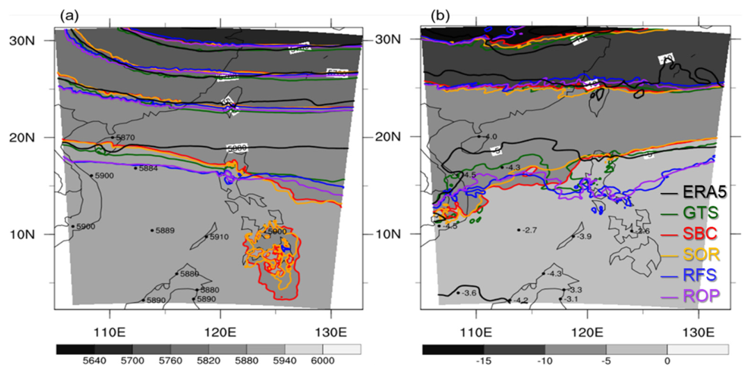
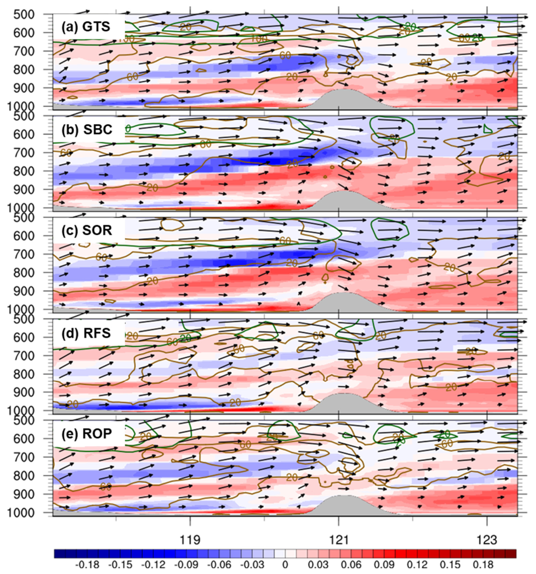
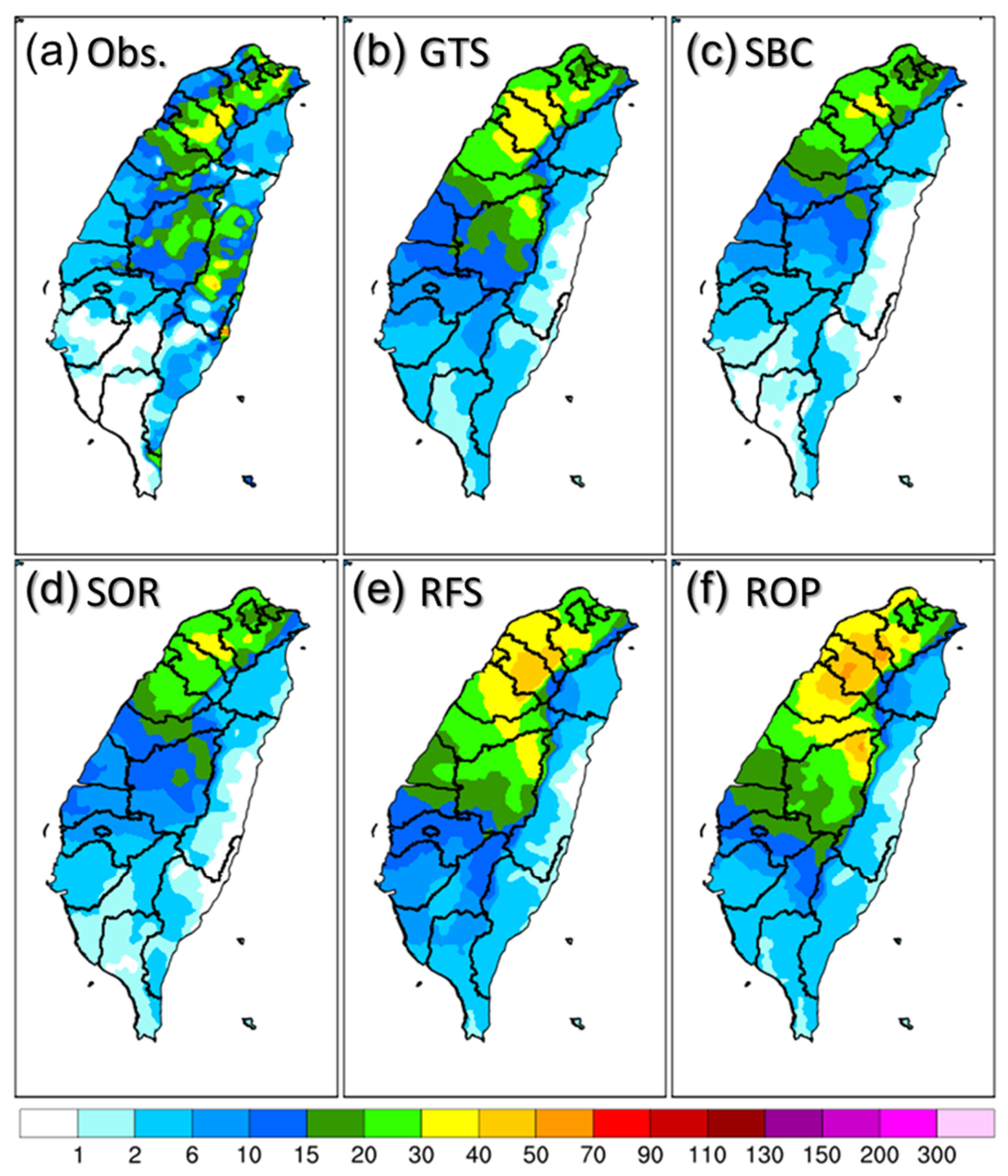
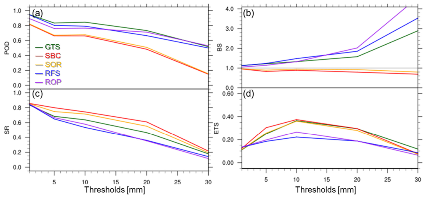
The geopotential height at 500 hPa is crucial to understanding weather and is affected by changes in temperature and moisture. Figure 14 presents the time-lag ensemble mean of geopotential height and temperature at 12Z on 11 April 2020. The heights in the RFS and ROP were nearly parallel to that recorded by the ERA5. However, the forecasts of the experiments underestimated both geopotential height and temperature. In addition, in the SBC and SOR, geopotential height was underestimated west of the 5880 line and overestimated in the eastern direction. As indicated by the temperature field (Figure 14b), in the SBC and SOR, temperature was underestimated west of the −5° line but overestimated to the east. The misestimates along the −5° line refer to ERA5, whereas nearby RAOBs still show about −4°. This pattern indicates that the forecasts of the SBC and SOR were baroclinic. As presented in Figure 15b,c, the magnitude of the vertical gradient of the equivalent potential temperature ( θ e p ) increased. The tilted structure from the west extended to Taiwan and involved a terrain-forced updraft between 120°E and 121°E. This updraft carried water vapor at a high level, where substantial amounts of liquid and solid water were condensed. The dry bias of the NSND caused the forecast of the SOR to indicate weak condensation and a small amount of liquid and solid water (Figure 15c). By contrast, the high concentration of vapor at low levels in the RFS and ROP forecasts led to updrafts over the ocean (from 117°E to 120.5°E), as depicted in Figure 15d,e. Water vapor readily condensed at low levels, producing heavy rainfall (Figure 16e,f). Rainfall occurred in the northwest and central east of Taiwan, and no rain was noted in the southwest (Figure 16a). The maximum amount of rainfall was approximately 30 mm. GTS overestimates the precipitation in the southwest (Figure 16b), shows little rainfall in the east, and overestimates in the northwest. In contrast, SBC more accurately captures the rainfall pattern in the southwest (Figure 16c), though it similarly underestimates the precipitation in the east, while its performance in the northwest aligns much closer with observations. SOR shows a spatial distribution closely resembling SBC but with higher rainfall intensities (Figure 16d). The RFS and ROP forecasts overestimated the amount of rainfall in Taiwan (Figure 16e,f), presenting values of approximately 40 and 50 mm, respectively. This study employed the probability of detection (POD), bias score (BS), and success ratio (SR) from [47], along with the equitable threat score (ETS) proposed by [48], to evaluate rainfall performance as follows (Table 2):
P O D = Y Y Y Y + N Y
B S = Y Y + Y N Y Y + N Y
S R = Y Y Y Y + Y N
R = ( Y Y + Y N ) × ( Y Y + N Y ) T o t a l
E T S = Y Y R Y Y + N Y R
While GTS, RFS, and ROP achieve a higher POD (Figure 17), they suffer from severe frequency overestimation (BS > 2.0) and a lower SR at higher thresholds. In contrast, SBC and SOR maintain a well-balanced frequency bias (BS close to 1.0) and higher SR, even with a lower POD for heavy precipitation. Overall, the ETS highlights that the SBC, GTS, and SOR deliver the highest prediction skill, peaking at the 10 mm threshold, whereas the excessive false alarms in RFS and ROP significantly degrade their overall forecast performance. The SBC forecast presented the most favorable rainfall pattern (Figure 16c) and had the highest ETS (Figure 17d). It should be emphasized that the lower prediction skill and severe moisture overestimation observed in the RFS and ROP experiments do not imply an inherent limitation of radiance assimilation itself. Because the radiance experiments in this study utilized NCEP global bias correction coefficients as a standard baseline, they lacked regional tuning tailored to the specific transition-season environment of Taiwan. The results here should be interpreted as a cautious reminder for regional modelers regarding the sensitivity of radiance bias correction, rather than a generalized conclusion that sounding assimilation inherently outperforms regional radiance assimilation.
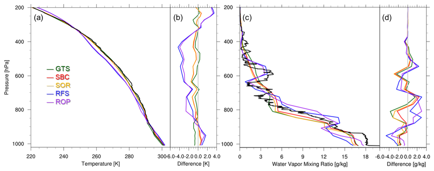
This study also analyzed radiosonde obtained from R/V Legend at 06Z on 15 April under clear-sky conditions. The radiosonde observations were used only for analysis and were not included in the data assimilation. The temperature and water vapor mixing ratio results were classified into radiance and NSND groups (Figure 18). Compared with those in the radiance group, the results in the NSND group exhibited a smaller temperature difference after assimilation and were closer to the observations from R/V Legend. However, the accuracy of the SBC forecast was slightly lower than that of the SOR. Whereas the GTS forecast differed the least in temperature from the observations, the SBC forecast differed the least in the water vapor mixing ratio. Between 550 and 650 hPa, the SBC and SOR forecasts did not indicate higher water vapor mixing ratios than those in the actual observations, indicating that the retrievals did not reveal this pattern. By contrast, the radiance group had relatively high values. Between 750 hPa and the surface, the NSNDs were generally consistent with the observations of R/V Legend but were slightly drier. The wet boundary layer in the radiance group was higher than that in the observations.
Assimilation of objectively bias-corrected NSNDs led to initial conditions in forecasts that were thermodynamically consistent with actual observations. This consistency positively contributed to the representation of frontal baroclinity and substantially improved the performance of quantitative precipitation forecasting model.

4. Discussion

Meteorological satellite-retrieved profiles, particularly those obtained from synergistic hyperspectral infrared and advanced microwave sounders, provide data regarding atmospheric thermodynamic states. These data can be used to improve the initial and boundary conditions for NWP models through the application of data assimilation. Multiple studies have indicated that observed radiances have a positive influence on weather forecasting and simulations. However, the first guess in the retrieval process may not accurately represent an atmospheric state, which can lead to inaccurate temperature and moisture profile estimations. In addition, the presence of clouds in the FOR may lead to systematic bias. To address these problems, this study proposed an objective quality control and cloud-dependent correction method.
The NSND was selected to investigate the proper method, and it was found that the quality of the NSND dependence on the cloud and land fractions within the FOR. Atmospheric temperature profiles under the pressure level of clouds and over land have the largest uncertainty and should not be adopted. After these criteria were applied, the RMSD between the results of the proposed model and the data of the ERA5 decreased from 3.3 to 1.3 K. The retrieved moisture profiles at each altitude level have the relative cloud-top height estimated as the RCTL and can be used to identify the bias and relationship with the RCTL. When these RCTL criteria and biases were applied, the bias in predicting the water vapor mixing ratio decreased from −8.7% to −0.7% in the study area. This decrease led to unbiased and reasonable predictions of temperature and moisture profiles from the NSND. The results from the IASI indicate that bias correction should be performed separately for each sensor.
These unbiased profiles were assimilated into an NWP model, and several experiments were conducted to evaluate the impact of bias correction and operational radiance assimilation. This study confirmed the utility of its model by considering the case of a spring front in Taiwan that occurred on 11 April 2020. The study conducted forecasting experiments, and the results indicated that employing corrected NSND improved the ability to forecast water vapor ratios. In all experiments, the precipitation ETS reached 0.4. Although SBC is relatively optimal, the absolute scores are low. The forecast in transition season still faces challenges. Furthermore, this study compared the use of the NSND and that of radiance in the proposed model. The NSND experiment revealed an enhanced baroclinic front feature, whereas the radiance assimilation experiment overestimated water vapor condensation and weaker baroclinity. The radiance experiment also overestimated rainfall because of the excessive condensation of water vapor. It is worth noting that the radiance assimilation experiments in this study were configured using NCEP global bias correction coefficients to represent a standard baseline scenario, ingesting operational products directly from major weather centers without localized regional adjustments. The lower performance or moisture biases observed in RFS/ROP should be interpreted as a cautious reminder for regional modelers rather than an inherent limitation of radiance assimilation itself.
Recent updates (Appendix A) demonstrate that incorporating shortwave infrared data and refining surface emissivity improve NUCAPS’s temperature quality and stability, needing only minimal outlier removal. However, water vapor still suffers from a dry bias, which remains effectively resolved by our proposed RCTL bias correction method.
In summary, meteorological satellite soundings are crucial in NWP, and incorporating adjusted data regarding atmospheric states in such models can achieve comparable results to incorporating radiances. The proposed method for assimilation requires few resources and it facilitates the quantification of observation-error covariance. Future studies should validate the method in models involving weather phenomena of different spatial scales, such as thunderstorms, typhoons, and atmospheric rivers.

5. Conclusions

This study developed and validated an objective quality control and cloud-dependent bias correction method for the NUCAPS sounding product to optimize its application in NWP. By categorizing retrieval uncertainties based on cloud and surface fractions, we successfully established filtering thresholds that reduced temperature retrieval profiles’ RMSD from 3.3 K to 1.3 K. Concurrently, the implementation of an RCTL-dependent lookup table systematically corrected the dry bias near cloud tops, reducing the water vapor mixing ratio bias closer to 0%.
Data assimilation experiments based on a transition-season front case in Taiwan confirmed that the objectively corrected sounding data generated forecast fields highly consistent with observations. This thermodynamic consistency enhanced the model’s capability to capture frontal baroclinity, yielding the most accurate quantitative precipitation forecast compared to conventional observations and the baseline radiance experiments without regional calibration. Although corrected sounding got the highest ETS, a score of 0.4 still shows that it remains challenging for transition-season cases.

Author Contributions

Conceptualization, K.-S.C., C.-Y.L., and S.-C.H.; Methodology, S.-C.H.; Software, S.-C.H.; Validation, S.-C.H.; Formal Analysis, C.-Y.L. and S.-C.H.; Writing—Original Draft, C.-Y.L. and S.-C.H.; Writing—Review and Editing, C.-Y.L. and S.-C.H.; Visualization, S.-C.H.; Funding Acquisition, Y.-C.S., C.-B.C., Y.-C.C. (Yu-Chun Chen) and Y.-C.C. (Yu-Cheng Chang). All authors have read and agreed to the published version of the manuscript.

Funding

This study was jointly supported by the National Science and Technology Council of Taiwan (grant nos. NSTC 114--2119--M--001--007, NSTC 114--2740--M--001--002, NSTC 114--2111--M--001--01, and NSTC 115-2111-M-001-010) and by Academia Sinica (project no. AS--IAIA--114--M03).

Data Availability Statement

Raw data supporting the conclusions of this study are available from the authors upon reasonable request.

Acknowledgments

The authors would like to thank the Taiwan Central Weather Administration for providing observational data, the operators of R/V Legend for providing radiosonde data, and the National Oceanic and Atmospheric Administration for providing NSND data.

Conflicts of Interest

The authors declare no conflicts of interest.

Appendix A

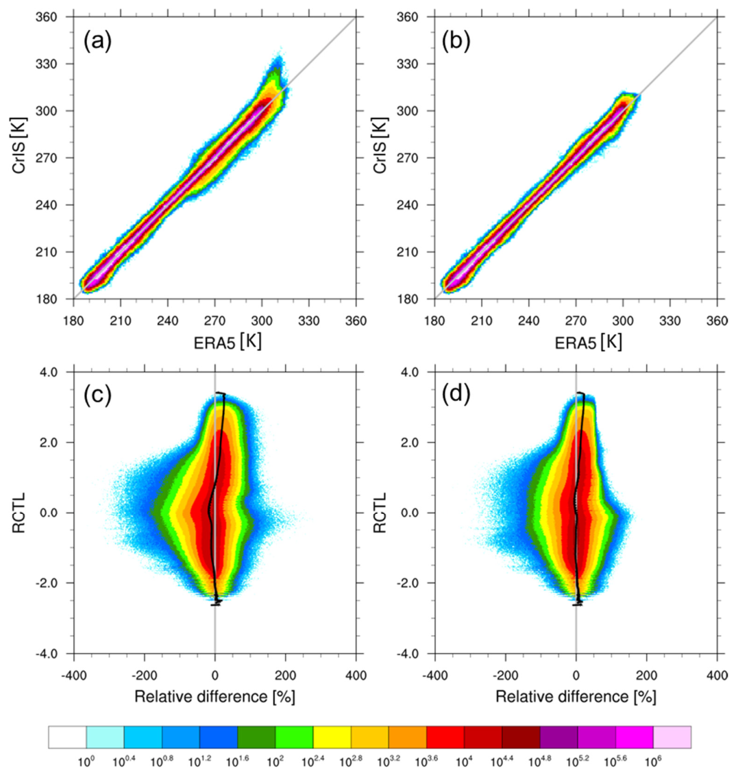
CrIS and ERA5 data from June 2025 to May 2026 were collected to evaluate the quality of the recent SND product and to test the quality control and bias correction methods proposed in this study. Over the past years, the NUCAPS has transitioned into advanced versions within the Hyperspectral Enterprise Algorithm Package to expand its atmospheric composition capabilities. A major milestone was the operational implementation of Averaging Kernels, providing users with essential indicators of vertical sensitivity and information content for greenhouse and trace gases [49,50,51,52]. The updates integrated optimized a priori datasets, while refining surface emissivity and effective reflectivity variables within the retrieval state vector to correct [52]. The update of the Community Radiative Transfer Model, the operator of NUCAPS, has been shown to improve the simulation of CrIS shortwave infrared observations, thereby also improving the increment statistics from applicable CrIS shortwave infrared channels [22,53,54].
For the original atmospheric temperature, the SND product shows significant improvement, with the high uncertainties previously associated with land data no longer existing [22]. However, a warm bias remains within the 300–330 K range, which required the application of QC to remove extreme outliers. Regarding atmospheric water vapor, a dry bias is shown in the raw data, which can be effectively correct using the lookup table (Y) statistically derived from October 2019 to September 2020 data. The small bias indicates that the Y function remains applicable over multiple years.
Figure A1. Two-dimensional frequency histograms of atmospheric temperature [K] for CrIS and ERA5 (a) before and (b) after quality control. Panels (c,d) show the two-dimensional frequency histograms of the relative difference [%] between CrIS and ERA5 as a function of RCTL, (c) before and (d) after bias correction. All data span from June 2025 to May 2026.
Remotesensing 18 02549 g0a1

References

  1. Kalnay, E.; Kanamitsu, M.; Kistler, R.; Collins, W.; Deaven, D.; Gandin, L.; Iredell, M.; Saha, S.; White, G.; Woollen, J.; et al. The NCEP/NCAR 40-Year Reanalysis Project. In Renewable Energy; Routledge: Abingdon, UK, 1996. [Google Scholar]
  2. Eyre, J.R.; Bell, W.; Cotton, J.; English, S.J.; Forsythe, M.; Healy, S.B.; Pavelin, E.G. Assimilation of Satellite Data in Numerical Weather Prediction. Part II: Recent Years. Q. J. R. Meteorol. Soc. 2022, 148, 521–556. [Google Scholar] [CrossRef] [Scilit]
  3. Zhang, Y.; Chen, X.; Stensrud, D.J.; Clothiaux, E.E. Enhancing Severe Weather Prediction with Microwave All-Sky Radiance Assimilation: The 10 August 2020 Midwest Derecho. Geophys. Res. Lett. 2024, 51, e2023GL106602. [Google Scholar] [CrossRef] [Scilit]
  4. Bell, B.; Thépaut, J.; Eyre, J. The Assimilation of Satellite Data in Numerical Weather Prediction Systems. In Satellites for Atmospheric Sciences 2; Wiley: Hoboken, NJ, USA, 2023; pp. 69–95. [Google Scholar]
  5. Liu, C.Y.; Kuo, S.C.; Lim, A.H.N.; Hsu, S.C.; Tseng, K.H.; Yeh, N.C.; Yang, Y.C. Optimal Use of Space-Borne Advanced Infrared and Microwave Soundings for Regional Numerical Weather Prediction. Remote Sens. 2016, 8, 816. [Google Scholar] [CrossRef] [Scilit]
  6. Menzel, W.P.; Schmit, T.J.; Zhang, P.; Li, J. Satellite-Based Atmospheric Infrared Sounder Development and Applications. Bull. Am. Meteorol. Soc. 2018, 99, 583–603. [Google Scholar] [CrossRef] [Scilit]
  7. Aryastana, P.; Liu, C.; Jong-Dao Jou, B.; Cayanan, E.; Punay, J.P.; Chen, Y. Assessment of Satellite Precipitation Data Sets for High Variability and Rapid Evolution of Typhoon Precipitation Events in the Philippines. Earth Space Sci. 2022, 9, e2022EA002382. [Google Scholar] [CrossRef] [Scilit]
  8. Singh, A.K.; Singh, V. Assessing the Accuracy and Reliability of Satellite-Derived Precipitation Products in the Kosi River Basin (India). Environ. Monit. Assess. 2024, 196, 671. [Google Scholar] [CrossRef] [Scilit] [PubMed]
  9. Wu, X.; Li, J.; Huang, A.; Menzel, P. Evaluation of Broadband and Hyperspectral IR Sounders. In Atmospheric and Environmental Remote Sensing Data Processing and Utilization: Numerical Atmospheric Prediction and Environmental Monitoring; Huang, H.-L.A., Bloom, H.J., Xu, X., Dittberner, G.J., Eds.; SPIE: Bellingham, WA, USA, 2005; p. 589005. [Google Scholar]
  10. Divakarla, M.G.; Barnet, C.D.; Goldberg, M.D.; McMillin, L.M.; Maddy, E.; Wolf, W.; Zhou, L.; Liu, X. Validation of Atmospheric Infrared Sounder Temperature and Water Vapor Retrievals with Matched Radiosonde Measurements and Forecasts. J. Geophys. Res. Atmos. 2006, 111, D09S15. [Google Scholar] [CrossRef] [Scilit]
  11. Smith, W.L.; Revercomb, H.; Bingham, G.E.; Larar, A.; Huang, H.; Li, J.; Liu, X.; Kireev, S. Evolution, Current Capabilities, and Advances in Satellite Ultra-spectral IR Sounding. AIP Conf. Proc. 2009, 1100, 335–338. [Google Scholar] [CrossRef] [Scilit]
  12. Liu, C.-Y.; Liu, G.-R.; Lin, T.-H.; Liu, C.-C.; Ren, H.; Young, C.-C. Using Surface Stations to Improve Sounding Retrievals from Hyperspectral Infrared Instruments. IEEE Trans. Geosci. Remote Sens. 2014, 52, 6957–6963. [Google Scholar] [CrossRef] [Scilit]
  13. Bauer, P.; Geer, A.J.; Lopez, P.; Salmond, D. Direct 4D-Var Assimilation of All-Sky Radiances. Part I: Implementation. Q. J. R. Meteorol. Soc. 2010, 136, 1868–1885. [Google Scholar] [CrossRef] [Scilit]
  14. Cardinali, C. Monitoring the Observation Impact on the Short-range Forecast. Q. J. R. Meteorol. Soc. 2009, 135, 239–250. [Google Scholar] [CrossRef] [Scilit]
  15. Geer, A.J.; Lonitz, K.; Weston, P.; Kazumori, M.; Okamoto, K.; Zhu, Y.; Liu, E.H.; Collard, A.; Bell, W.; Migliorini, S.; et al. All-sky Satellite Data Assimilation at Operational Weather Forecasting Centres. Q. J. R. Meteorol. Soc. 2018, 144, 1191–1217. [Google Scholar] [CrossRef] [Scilit]
  16. Le Marshall, J.; Jung, J.; Derber, J.; Chahine, M.; Treadon, R.; Lord, S.J.; Goldberg, M.; Wolf, W.; Liu, H.C.; Joiner, J.; et al. Improving Global Analysis and Forecasting with AIRS. Bull. Am. Meteorol. Soc. 2006, 87, 891–895. [Google Scholar] [CrossRef] [Scilit]
  17. Duruisseau, F.; Chambon, P.; Guedj, S.; Guidard, V.; Fourrié, N.; Taillefer, F.; Brousseau, P.; Mahfouf, J.; Roca, R. Investigating the Potential Benefit to a Mesoscale NWP Model of a Microwave Sounder on Board a Geostationary Satellite. Q. J. R. Meteorol. Soc. 2017, 143, 2104–2115. [Google Scholar] [CrossRef] [Scilit]
  18. McCarty, W.; Jedlovec, G.; Miller, T.L. Impact of the Assimilation of Atmospheric Infrared Sounder Radiance Measurements on Short-term Weather Forecasts. J. Geophys. Res. Atmos. 2009, 114, D18122. [Google Scholar] [CrossRef] [Scilit]
  19. Pu, Z.; Zhang, L. Validation of Atmospheric Infrared Sounder Temperature and Moisture Profiles over Tropical Oceans and Their Impact on Numerical Simulations of Tropical Cyclones. J. Geophys. Res. Atmos. 2010, 115, 24114. [Google Scholar] [CrossRef] [Scilit]
  20. Zheng, J.; Li, J.; Schmit, T.J.; Li, J.; Liu, Z. The Impact of AIRS Atmospheric Temperature and Moisture Profiles on Hurricane Forecasts: Ike (2008) and Irene (2011). Adv. Atmos. Sci. 2015, 32, 319–335. [Google Scholar] [CrossRef] [Scilit]
  21. Migliorini, S. On the Equivalence between Radiance and Retrieval Assimilation. Mon. Weather Rev. 2012, 140, 258–265. [Google Scholar] [CrossRef] [Scilit]
  22. Barnet, C.D.; Smith, N.; Ide, K.; Garrett, K.; Jones, E. Evaluating the Value of CrIS Shortwave-Infrared Channels in Atmospheric-Sounding Retrievals. Remote Sens. 2023, 15, 547. [Google Scholar] [CrossRef] [Scilit]
  23. Bauer, P. Sources of Biases in Microwave Radiative Transfer Modelling. Available online: https://www.ecmwf.int/sites/default/files/elibrary/2005/15837-sources-biases-microwave-radiattive-transfer-modelling.pdf (accessed on 8 June 2026).
  24. Li, Z.-L.; Wu, H.; Wang, N.; Qiu, S.; Sobrino, J.A.; Wan, Z.; Tang, B.-H.; Yan, G. Land Surface Emissivity Retrieval from Satellite Data. Int. J. Remote Sens. 2013, 34, 3084–3127. [Google Scholar] [CrossRef] [Scilit]
  25. Xie, Y.; Huang, X.; Chen, X.; L’Ecuyer, T.S.; Drouin, B.J.; Wang, J. Retrieval of Surface Spectral Emissivity in Polar Regions Based on the Optimal Estimation Method. J. Geophys. Res. Atmos. 2022, 127, e2021JD035677. [Google Scholar] [CrossRef] [Scilit]
  26. Liu, C.; Li, J.; Weisz, E.; Schmit, T.J.; Ackerman, S.A.; Huang, H. Synergistic Use of AIRS and MODIS Radiance Measurements for Atmospheric Profiling. Geophys. Res. Lett. 2008, 35, L21802. [Google Scholar] [CrossRef] [Scilit]
  27. Várnai, T.; Marshak, A. Statistical Analysis of the Uncertainties in Cloud Optical Depth Retrievals Caused by Three-Dimensional Radiative Effects. J. Atmos. Sci. 2001, 58, 1540–1548. [Google Scholar] [CrossRef] [Scilit]
  28. Bauer, P.; Auligné, T.; Bell, W.; Geer, A.; Guidard, V.; Heilliette, S.; Kazumori, M.; Kim, M.; Liu, E.H.-C.; McNally, A.P.; et al. Satellite Cloud and Precipitation Assimilation at Operational NWP Centres. Q. J. R. Meteorol. Soc. 2011, 137, 1934–1951. [Google Scholar] [CrossRef] [Scilit]
  29. Susskind, J.; Barnet, C.D.; Blaisdell, J.M. Retrieval of Atmospheric and Surface Parameters from AIRS/AMSU/HSB Data in the Presence of Clouds. IEEE Trans. Geosci. Remote Sens. 2003, 41, 390–409. [Google Scholar] [CrossRef] [Scilit]
  30. Barnet, C.; Manning, E.; Rosenkranz, P.; Strow, L.; Susskind, J.; Chahine, G.M.T. AIRS-Team Retrieval for Core Products and Geophysical Parameters Level 2; NASA: Washington, DC, USA, 2007.
  31. Barnet, C.D.; Divakarla, M.; Gambacorta, A.; Iturbide-Sanchez, F.; Nalli, N.R.; Pryor, K.; Tan, C.; Wang, T.; Warner, J.; Zhang, K.; et al. NOAA Unique Combined Atmospheric Processing System (NUCAPS) Algorithm Theoretical Basis Document. In AGU Fall Meeting Abstracts; American Geophysical Union (AGU): Washington, DC, USA, 2021. [Google Scholar]
  32. Jones, T.A.; Stensrud, D.J. Assimilating AIRS Temperature and Mixing Ratio Profiles Using an Ensemble Kalman Filter Approach for Convective-Scale Forecasts. Weather Forecast. 2012, 27, 541–564. [Google Scholar] [CrossRef] [Scilit]
  33. Raju, A.; Parekh, A.; Kumar, P.; Gnanaseelan, C. Evaluation of the Impact of AIRS Profiles on Prediction of Indian Summer Monsoon Using WRF Variational Data Assimilation System. J. Geophys. Res. 2015, 120, 8112–8131. [Google Scholar] [CrossRef] [Scilit]
  34. Esmaili, R.B.; Smith, N.; Berndt, E.B.; Dostalek, J.F.; Kahn, B.H.; White, K.; Barnet, C.D.; Sjoberg, W.; Goldberg, M. Adapting Satellite Soundings for Operational Forecasting within the Hazardous Weather Testbed. Remote Sens. 2020, 12, 886. [Google Scholar] [CrossRef] [Scilit]
  35. Chen, S.-Y.; Liu, C.-Y.; Huang, C.-Y.; Hsu, S.-C.; Li, H.-W.; Lin, P.-H.; Cheng, J.-P.; Huang, C.-Y. An Analysis Study of FORMOSAT-7/COSMIC-2 Radio Occultation Data in the Troposphere. Remote Sens. 2021, 13, 717. [Google Scholar] [CrossRef] [Scilit]
  36. Wang, C.-C.; Sung, Y.-T.; Liu, C.-Y.; Chang, C.-S.; Tsuboki, K.; Hsu, S.-C. The Impacts of Hyperspectral Infrared Sounding Assimilation for Cloud-Resolving Model Quantitative Precipitation Forecasts in Taiwan Mei-Yu Rainfall Events. Atmos. Res. 2026, 330, 108504. [Google Scholar] [CrossRef] [Scilit]
  37. Kuciauskas, A.; Reale, A.; Esmaili, R.; Sun, B.; Nalli, N.R.; Morris, V.R. Investigating NUCAPS Skill in Profiling Saharan Dust for Near-Real-Time Forecasting. Remote Sens. 2022, 14, 4261. [Google Scholar] [CrossRef] [Scilit]
  38. Singh, R.; Kishtawal, C.M.; Ojha, S.P.; Pal, P.K. Impact of Assimilation of Atmospheric InfraRed Sounder (AIRS) Radiances and Retrievals in the WRF 3D-Var Assimilation System. J. Geophys. Res. Atmos. 2012, 117, D11107. [Google Scholar] [CrossRef] [Scilit]
  39. Wolf, W.; Liu, M.; Reale, T.; Sharma, A. NUCAPS: NOAA Unique Combined Atmospheric Processing System Environmental Data Record (EDR) Products. Available online: https://www.ncei.noaa.gov/access/metadata/landing-page/bin/iso?id=gov.noaa.ncdc:C00868 (accessed on 8 June 2026).
  40. Thrastarson, H.T.; Manning, E.; Kahn, B.; Fetzer, E.J.; Yue, Q.; Wong, S.; Kalmus, P.; Payne, V.; Wang, T.; Olsen, E.T.; et al. AIRS/AMSU/HSB Version 7 Level 2 Product User Guide. 2021. Available online: https://docserver.gesdisc.eosdis.nasa.gov/public/project/AIRS/V7_L2_Product_User_Guide.pdf (accessed on 8 June 2026).
  41. Toledo, D.; Córdoba-Jabonero, C.; Adame, J.A.; De La Morena, B.; Gil-Ojeda, M. Estimation of the Atmospheric Boundary Layer Height during Different Atmospheric Conditions: A Comparison on Reliability of Several Methods Applied to Lidar Measurements. Int. J. Remote Sens. 2017, 38, 3203–3218. [Google Scholar] [CrossRef] [Scilit]
  42. Chen, C.-S.; Chen, Y.-L. The Rainfall Characteristics of Taiwan. Mon. Weather Rev. 2003, 131, 1323–1341. [Google Scholar] [CrossRef] [Scilit]
  43. Zhang, C.; Wang, Y. Projected Future Changes of Tropical Cyclone Activity over the Western North and South Pacific in a 20-Km-Mesh Regional Climate Model. J. Clim. 2017, 30, 5923–5941. [Google Scholar] [CrossRef] [Scilit]
  44. Zhang, C.; Wang, Y.; Hamilton, K. Improved Representation of Boundary Layer Clouds over the Southeast Pacific in ARW-WRF Using a Modified Tiedtke Cumulus Parameterization Scheme. Mon. Weather Rev. 2011, 139, 3489–3513. [Google Scholar] [CrossRef] [Scilit]
  45. Morrison, H.; Thompson, G.; Tatarskii, V. Impact of Cloud Microphysics on the Development of Trailing Stratiform Precipitation in a Simulated Squall Line: Comparison of One- and Two-Moment Schemes. Mon. Weather Rev. 2009, 137, 991–1007. [Google Scholar] [CrossRef] [Scilit]
  46. Hong, S.-Y.; Noh, Y.; Dudhia, J. A New Vertical Diffusion Package with an Explicit Treatment of Entrainment Processes. Mon. Weather Rev. 2006, 134, 2318–2341. [Google Scholar] [CrossRef] [Scilit]
  47. Wilks, D.S. Statistical Methods in the Atmospheric Sciences; Academic Press: Cambridge, MA, USA, 2006. [Google Scholar]
  48. Schaefer, J.T. The Critical Success Index as an Indicator of Warning Skill. Weather Forecast. 1990, 5, 570–575. [Google Scholar] [CrossRef] [Scilit]
  49. Zhu, T.; Divakarla, M.; Pryor, K.; Petropavlovskikh, I.; Warner, J.; Wilson, M.; Nalli, N.R.; Tan, C.; Kulko, M.; Li, W.; et al. Improvement of Nucaps Ozone Retrieval and Validation with Averaging Kernel Analysis. In Proceedings of the IGARSS 2024—2024 IEEE International Geoscience and Remote Sensing Symposium, Athens, Greece, 7–12 July 2024; IEEE: New York, NY, USA, 2024; pp. 2979–2981. [Google Scholar]
  50. Nalli, N.R.; Tan, C.; Warner, J.; Divakarla, M.; Gambacorta, A.; Wilson, M.; Zhu, T.; Wang, T.; Wei, Z.; Pryor, K.; et al. Validation of Carbon Trace Gas Profile Retrievals from the NOAA-Unique Combined Atmospheric Processing System for the Cross-Track Infrared Sounder. Remote Sens. 2020, 12, 3245. [Google Scholar] [CrossRef] [Scilit]
  51. Warner, J.; Wei, Z.; Divakarla, M.G.; Pryor, K.L.; Nalli, N.R.; Tan, C.; Zhu, T.; Wilson, M.; Zhou, L.; Kalluri, S. Recent Algorithm Updates to the NUCAPS Greenhouse Gas Products and Inter-Comparison to Other Satellite Products. In Proceedings of the 103rd Annual AMS Meeting 2023, Denver, CO, USA, 8–12 January 2023; AMS: Boston, MA, USA, 2023; Volume 103, p. 424. [Google Scholar]
  52. Divakarla, M.G.; Pryor, K.L.; Zhu, T.; Warner, J.; Kulko, M.; Nalli, N.R.; Wilson, M.; Soulliard, L. NUCAPS Hyperspectral Infrared Atmospheric Sounding Products: Recent Algorithm Improvements and Product Updates for JPSS-CrIS and MetOp-IASI. In Proceedings of the 104th Annual AMS Meeting 2024, Baltimore, MD, USA, 28 January–1 February 2024; AMS: Boston, MA, USA, 2024; Volume 104, p. 431406. [Google Scholar]
  53. Jones, E.; Garrett, K.; Ide, K.; Ma, Y.; Karpowicz, B.; Barnet, C.; Boukabara, S. Enabling the Assimilation of CrIS Shortwave Infrared Observations in Global NWP at NOAA. Part I: Background and Methods. J. Atmos. Ocean. Technol. 2024, 41, 1265–1276. [Google Scholar] [CrossRef] [Scilit]
  54. Smith, N.; Barnet, C.D. An Information Content Approach to Diagnosing and Improving CLIMCAPS Retrieval Consistency across Instruments and Satellites. Atmos. Meas. Tech. 2025, 18, 1823–1839. [Google Scholar] [CrossRef] [Scilit]
Figure 1. Two−dimensional atmospheric temperature [K] frequency histograms of the (a) CrIS and ERA5, (b) IASI and ERA5, (c) IASI and IGRA, (d) IGRA and ERA5, (e) CrIS after quality control and ERA5, and (f) IASI after quality control and ERA5. The solid lines represent the linear regression functions (black), diagonal line (gray).
Remotesensing 18 02549 g001
Figure 2. Two−dimensional frequency histograms of the retrieved atmospheric temperature and ERA5 temperature difference (CrIS minus ERA5, y−axis) against the ERA5 (x−axis): (a) pressure levels above the highest layer of clouds, (b) pressure levels between the two layers of clouds, (c) cloud layer misplacement, and (d) pressure levels below the lowest layer of clouds.
Remotesensing 18 02549 g002
Figure 3. Two−dimensional frequency histograms of the differences in the retrieved atmospheric temperatures and ERA5 temperatures (CrIS minus ERA5, y−axis) against the ERA5 (x−axis), with sample categorization into (a) ocean, (b) coastal, and (c) land regions.
Remotesensing 18 02549 g003
Figure 4. Flowchart of the procedure used for quality control of the retrieved atmospheric temperature data. The percentages represent the proportions of total matched NSNDs during October 2019 to September 2020.
Remotesensing 18 02549 g004
Figure 5. Two−dimensional frequency histogram of the water vapor mixing ratio [g/kg] between the (a) CrIS and ERA5, (b) IASI and ERA5, (c) IASI and IGRA, (d) IGRA and ERA5, (e) CrIS after quality control and ERA5, and (f) IASI after quality control and ERA5. The solid lines represent the linear regression functions (black), diagonal line (gray).
Remotesensing 18 02549 g005
Figure 6. Two−dimensional histogram of the water vapor RD between the CrIS and ERA5 (colored). The y−axis represents the logarithm of relative pressure from the highest cloud top pressure, and the x−axis represents the water vapor relative difference [%] relative to the ERA5 or IGRA. The colored solid curves represent the mean values for the difference between the CrIS and ERA5 (black), IASI and ERA5 (blue), and IASI and IGRA (green) at a given RCTL. The white solid curves represent one and two standard deviations at a given RCTL. Panel (a) presents the original NSND data against the ERA5 or IGRA, and panel (b) presents the data after bias correction.
Remotesensing 18 02549 g006
Figure 7. The Y (RCTL) distribution. Y is the lookup table for the bias correction coefficient, defined as the average of RD along the RCTL (black line in Figure 6a). It is set to 0 when the RCTL exceeds 1.5, indicating that no correction is applied.
Remotesensing 18 02549 g007
Figure 8. Composited surface front locations overlaid on a CWA weather map at 06Z on 10 April 2020. The front was located at 06Z on 10 April and at 00/06/12/18Z on 11 April. The black contours represent the sea level pressure at 06Z on 10 April.
Remotesensing 18 02549 g008
Figure 9. Hourly rainfall intensity [mm/h] in Taipei from 8 to 18 April 2020. The primary rain event in Taipei occurred from 06Z on 11 April to 06Z on 12 April (shading in the plot). The bold black vertical line represents the radiosonde released by R/V Legend at 12.569°N, 115.462°E at 06Z on 15 April.
Remotesensing 18 02549 g009
Figure 10. Areas in East Asia and the western North Pacific region (entire region) in which the effectiveness of data assimilation was analyzed. The grid resolution for the region is 27 km, and the inner domain (white box, d02) is 9 km. The sources of the radiosondes from the GTS, CWA, and R/V Legend are depicted as black, yellow, and red dots, respectively. The subregions analyzed in Figure 11 and Figure 14 are indicated using purple and blue boxes, respectively.
Remotesensing 18 02549 g010
Figure 11. A schematic illustration for model run. A cold start was implemented for the initial cycle of the spread experiments, utilizing a 12 h cycling window. Data assimilation was performed at 6 h intervals, followed by a 120 h forecast period.
Remotesensing 18 02549 g011
Figure 12. Time−lag ensemble MD of vertical velocity (indicated using color in a 10 2 m/s interval transitioning from blue to red), liquid water mixing ratio (brown contours), solid water mixing ratio (green contours), and precipitable water (black curves in the bottom subplot of each panel) over time (purple box in Figure 10). The positive (negative) differences between the liquid water mixing ratio and the solid water mixing ratio are indicated using solid (dashed) contour lines with a 1 g/kg interval. The vertical axis represents pressure in hectopascals. The horizontal axis represents forecasting time in hours; negative values represent the data assimilation window, and positive values represent forecasting hours. The bottom subplot of each panel represents total precipitable water in millimeters for the (a) SBC, (b) SOR, (c) RFS, and (d) ROP experiments.
Remotesensing 18 02549 g012
Figure 13. Time−lag ensemble MD (a) and RMSD (b) of temperature from 1000 to 200 hPa compared with radiosondes in the second domain in Figure 10 within 24 to 120 h of forecasting. The MRD and MARD of water vapor are presented in panels (c) and (d), respectively. The SBC, SOR, RFS, and ROP experiments are presented as red, orange, blue, and purple curves, respectively, and the GTS experiment is presented as a green curve.
Remotesensing 18 02549 g013
Figure 14. (a) Geopotential height [gpm] and (b) temperature [°C] at 500 hPa at 12Z on 11 April 2020. The bold black curves represent reference data obtained from the ERA5, and the dots with values represent data obtained from GTS radiosondes. The red curve and gray shading represent the results of the SBC experiment. The results of the SOR, RFS, and ROP experiments are labeled in orange, blue, and purple, respectively.
Remotesensing 18 02549 g014
Figure 15. Subdomain longitudinal mean of θ e p (colors, in K/hPa), liquid water vapor mixing ratio (brown contours from 20 to 100 per 40 g/kg), solid water vapor mixing ratio (green contours from 20 to 100 per 40 g/kg), and terrain (gray area) as indicated by the blue box in Figure 10 at 12Z on 11 April 2020. The arrows represent composited horizontal wind speed and 100 times of vertical velocity in meters per second. Panels (a), (b), (c), (d), and (e) represent the GTS, SBC, SOR, RFS, and ROP experiments, respectively.
Remotesensing 18 02549 g015
Figure 16. Accumulated rainfall [mm] observed (a) from 04Z on 11 April to 04Z on 12 April 2020. Panels (b), (c), (d), (e), and (f) present rainfall accumulation over this period in the GTS, SBC, SOR, RFS, and ROP experiments, respectively.
Remotesensing 18 02549 g016
Figure 17. (a) POD, (b) BS, (c) SR, and (d) ETS at different thresholds from 5 to 30 mm during the rainfall accumulation window from 04Z on 11 April to 04Z on 12 April 2020. The data for the GTS, SBC, SOR, RFS, and ROP experiments are represented as green, red, orange, blue, and purple curves, respectively.
Remotesensing 18 02549 g017
Figure 18. Analysis of (a) temperature and (c) water vapor mixing ratio. The GTS (green), SBC (red), SOR (orange), RFS (blue), and ROP (purple) forecasts are overlaid with radiosonde data from R/V Legend (black) at 06Z on 15 April 2020, as labeled in Figure 9. Panels (b,d) present the analysis without R/V Legend’s radiosondes of temperature and the water vapor mixing ratio.
Remotesensing 18 02549 g018
Table 1. Experiments involving assimilated data for sensitivity analysis.
ExperimentAssimilated Data
GTSGTS only
SBCGTS and quality controlled and bias corrected NSND
SORGTS and original NSND
RFSGTS and full spectral radiance
ROPGTS and operational channel radiance
Table 2. Contingency table used for verification of dichotomous forecasts and observations.
ForecastObservationTotal
YesNo
YesHits (YY)False alarms (YN)YY + YN
NoMisses (NY)Correct rejections (NN)NY + NN
TotalYY + NYYN + NNTotal = YY + YN + NY + NN
Disclaimer/Publisher’s Note: The statements, opinions and data contained in all publications are solely those of the individual author(s) and contributor(s) and not of MDPI and/or the editor(s). MDPI and/or the editor(s) disclaim responsibility for any injury to people or property resulting from any ideas, methods, instructions or products referred to in the content.