Aliasing Suppression in Synthetic Aperture Interferometric Radiometers Using Subarray-Based Antenna Architecture

Highlights

What are the main findings?

• A subarray-based antenna architecture is proposed to suppress aliasing artifacts in synthetic aperture interferometric radiometers by aligning subarray pattern nulls with sparse array grating lobe directions.
• The proposed method reduces grating lobe levels and aliasing artifacts while maintaining competitive spatial resolution and radiometric sensitivity.

What are the implications of the main findings?

• The proposed architecture provides a practical approach for mitigating aliasing effects in SAIR systems without requiring additional receiving channels or post processing.
• The analysis of subarray configurations and direction dependent suppression characteristics provides guidance for SAIR antenna design under sparse spatial frequency sampling.

Abstract

Synthetic aperture interferometric radiometers (SAIRs) have emerged as a promising technology for high-resolution remote sensing and target detection by synthesizing spatially distributed antenna elements into a large virtual aperture. To achieve high angular resolution and radiometric sensitivity, SAIR systems often employ sparse antenna arrays composed of antenna elements with large apertures and high gain, resulting in element spacings exceeding half a wavelength. Such undersampling violates the Nyquist sampling criterion, generating grating lobes in the array factor (AF) and resulting in spatial aliasing artifacts in reconstructed brightness temperature (TB) images, which degrade imaging and detection performance. To mitigate this problem, this paper proposes an aliasing suppression method based on a subarray-based antenna architecture. First, the grating lobe directions of the sparse array are identified through AF analysis. Each conventional antenna element is then replaced with a properly designed subarray antenna whose radiation pattern introduces nulls are placed near the grating lobe directions, thereby reducing the corresponding aliasing artifacts in reconstructed TB images. Simulation results and an equivalent experimental emulation demonstrate that the proposed method reduces aliasing artifacts while maintaining competitive spatial resolution and radiometric sensitivity. Additional analyses investigate the effects of subarray layout, the number of subarray elements, and wideband operation, as well as the direction dependence of grating lobe suppression, providing practical guidance for SAIR system design.

1. Introduction

Synthetic aperture interferometric radiometers (SAIRs) are passive microwave remote sensing instruments that reconstruct brightness temperature (TB) distributions from measured visibilities. By synthesizing a large virtual aperture, SAIRs achieve high spatial resolution with a compact physical configuration compared with conventional real-aperture radiometers. In addition, they provide instantaneous imaging capability with all-weather and day-and-night observation [1,2,3]. These advantages have attracted increasing interest in SAIR technology for Earth observation applications and target detection [4,5,6,7,8].

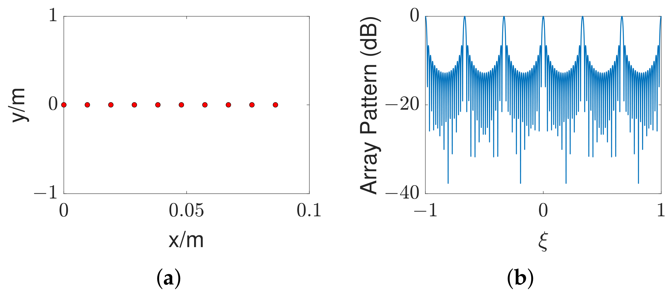
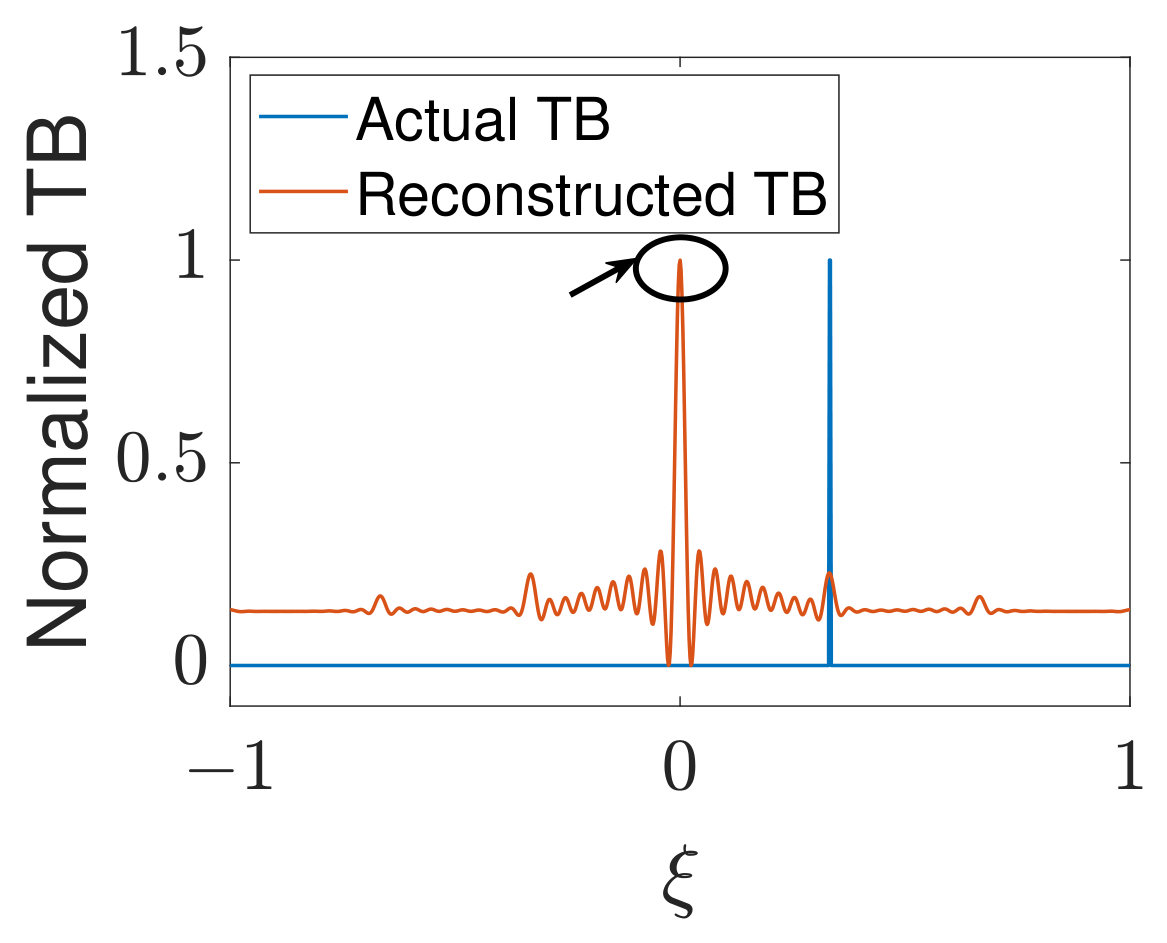
Target detection using SAIR relies on the TB contrast between the target and the background. In general, higher angular resolution and radiometric sensitivity improve detection performance [7]. To achieve these requirements, SAIR systems often employ sparse antenna arrays composed of antenna elements with large apertures and high gain. However, the resulting element spacing may exceed half a wavelength [1,9,10,11]. Such undersampling violates the Nyquist sampling criterion and produces grating lobes in the array factor (AF). These grating lobes introduce periodic spatial aliasing artifacts in the reconstructed TB images, which may degrade imaging reliability and detection performance. Consequently, the suppression of grating lobes and spatial aliasing has become an important research topic in SAIR systems.

Existing approaches for suppressing grating lobes in SAIR systems can be broadly categorized into two groups: array-configuration-based approaches and post-processing-based approaches.

The first group aims to suppress grating lobes through array configuration design and can be further divided into uniform and nonuniform array strategies. For uniform-array-based designs, Zhang et al. [11] employed three smaller antennas, each with half the diameter of the original elements, to achieve shorter baselines, thereby improving low-frequency coverage and spatial frequency sampling. However, this design increases system complexity and introduces challenges such as inconsistent antenna responses. In addition, a beamforming-based radiometer with steerable elements was proposed in [12], which enables more flexible beam pattern control. However, its effectiveness is limited to narrow bandwidths and requires highly accurate beamforming control. From a hardware-cost perspective, Zheng et al. [13] proposed a uniform linear array that doubles the effective field of view (FOV) at the expense of degraded angular resolution and unsatisfactory imaging performance for extended targets. Alternatively, nonuniform array designs redistribute grating lobe energy to reduce aliasing artifacts [14,15]. However, as the element spacing increases, strong sparsity still leads to high sidelobes. Moreover, the design of large-scale nonuniform arrays becomes increasingly challenging, and the resulting irregular spatial frequency sampling typically requires dedicated reconstruction algorithms.

The second group includes post-processing techniques, mainly based on interpolation and weighting schemes. Interpolation methods [9,16] enhance the spatial frequency sampling by estimating intermediate visibility samples, thereby reducing imaging artifacts. However, interpolation may introduce residual errors. Weighting schemes have also been investigated to suppress sidelobes. For instance, Peng et al. [17] proposed an adaptive weighting method that reduces sidelobes in the reconstructed image. Nevertheless, such approaches increase computational complexity and may limit their applicability in large-scale real-time SAIR systems.

In summary, array-configuration-based approaches often increase system complexity due to the need for additional antennas, channels, or correlators, and may lead to degraded angular resolution and imaging quality. Post-processing-based approaches are computationally expensive and may introduce residual errors.

To address these limitations, this paper proposes an aliasing suppression method based on a subarray-based antenna architecture for SAIR systems. Instead of modifying the array configuration or relying on post-processing algorithms, the proposed approach exploits the additional degree of freedom in antenna pattern design. Specifically, the grating lobe directions of the sparse array are first identified through AF characterization. Then, a subarray-based antenna is designed such that its pattern introduces nulls aligned with these grating lobe directions. By replacing each conventional antenna element with the designed subarray-based antenna, aliasing artifacts can be suppressed while maintaining competitive spatial resolution and radiometric sensitivity, without increasing the number of channels or correlators. Furthermore, the effects of several practical design factors are systematically investigated, including the subarray layout, the number of elements within each subarray, and the operating bandwidth. The direction dependence of the resulting suppression performance is also examined to provide practical guidance for SAIR system design.

It is important to clarify the relationship between the proposed subarray-based antenna architecture and subarray concepts in phased-array systems [18]. The proposed mechanism is related to the classical pattern multiplication principle, where the overall array response is jointly determined by the AF and the element or subarray pattern [18]. Therefore, using element or subarray pattern nulls to control grating lobes within a prescribed angular region has precedents in antenna array theory [19,20,21]. However, the present SAIR formulation differs from conventional phased-array in its operating mode and design objective. In phased-array systems, nulling is usually achieved by actively controlling the excitation amplitudes and phases of array elements or subarray ports to synthesize a desired beam pattern, such as beam steering, sidelobe reduction, or interference suppression. In contrast, SAIR systems operate in a passive mode, where cross-correlations between receiving channels are measured as visibilities and then inverted to reconstruct the TB distribution. Thus, the proposed method does not perform active beam synthesis. Instead, it uses a fixed passive subarray pattern to modulate the spatial response of the SAIR system at the antenna-pattern level, thereby attenuating contributions from grating lobe directions and reducing aliasing artifacts in reconstructed TB images. This design introduces an additional degree of freedom for element pattern control without altering the sparse array configuration or increasing the number of receiving channels, enabling system response shaping in SAIR systems. Accordingly, this work focuses on formulating and validating this mechanism within the SAIR visibility measurement and TB reconstruction framework.

The main contributions of this article are summarized as follows:

• This work introduces an element-level design degree of freedom for grating lobe suppression in sparse array SAIR systems. While pattern null placement is related to classical subarray and pattern multiplication theory, this work incorporates this mechanism into the SAIR visibility measurement and TB reconstruction framework. Specifically, the subarray-based antenna is designed to place pattern nulls near the grating lobe directions of the sparse array, so that the spatial response is attenuated in these directions. As a result, grating-lobe-induced aliasing artifacts are reduced in the reconstructed TB images without increasing the number of receiving channels or correlators.
• The proposed method is demonstrated using several representative array configurations. In addition, the effects of practical design factors, including subarray layout, the number of elements within each subarray, and wideband operation, are systematically analyzed, and the direction dependence of grating lobe suppression is further examined to provide practical design guidelines.

The remainder of this article is organized as follows: Section 2 introduces the principle and the performance metrics of SAIR systems. Section 3 analyzes grating lobes in sparse arrays and presents a subarray-based antenna design method. Section 4 presents numerical simulations and equivalent experimental validation of the proposed method, including array response analysis, imaging performance evaluation, and analyses of practical design factors such as subarray layout, element number, and wideband operation. The direction dependence of grating lobe suppression is further evaluated to provide a more complete assessment of the proposed design rule. Section 5 provides further discussion on the physical mechanism of the proposed method, its relation to classical subarray theory and existing SAIR approaches, and its practical implementation issues and limitations. Section 6 concludes the article.

2. Principles

2.1. Array Pattern of SAIRs

For an ideal SAIR system, the visibility function $V(u_{ij},v_{ij})$ in the far-field condition has the following relationship with the modified brightness temperature (TB) $T_M(\xi ,\eta )$ [22]:

$$\begin{array}{cc}\hfill V(u_{ij},v_{ij})=& \underset{{\xi }^2+{\eta }^2\le 1}{\int \int }{T}_M(\xi ,\eta )·e^{-j2\pi (u_{ij}\xi +v_{ij}\eta )}d\xi d\eta ,\hfill \end{array}$$

(1)

$$T_M(\xi ,\eta )={\int }_{-\infty }^{+\infty }{\int }_{-\infty }^{+\infty }V(u,v)·e^{j2\pi (u\xi +v\eta )}dudv,$$

(2)

with

$$\begin{array}{c}\hfill T_M(\xi ,\eta )={\displaystyle \frac{1}{\sqrt{{\mathsf{\Omega }}_i{\mathsf{\Omega }}_j}}}·{\displaystyle \frac{T_B(\xi ,\eta )}{\sqrt{1-{\xi }^2-{\eta }^2}}}·f_i(\xi ,\eta )·f_j^{\ast }(\xi ,\eta )·{\tilde{r}}_{ij}\left(-{\displaystyle \frac{(u_{ij}\xi +v_{ij}\eta )}{f_0}}\right),\end{array}$$

(3)

where $T_B(\xi ,\eta )$ denotes the scene TB, $(u_{ij},v_{ij})$ denotes the spatial frequency, $\lambda$ denotes the wavelength, $(\xi ,\eta )$ denotes the direction cosine, ${\mathsf{\Omega }}_i$ denotes the equivalent solid angle of the ith antenna, $f_i(\xi ,\eta )$ denotes the normalized voltage pattern of the ith antenna, ${\tilde{r}}_{ij}(·)$ denotes the fringe-washing function, and $1/\sqrt{1-{\xi }^2-{\eta }^2}$ denotes the obliquity factor.

For an actual SAIR system, the number of antennas is finite, then the sampled visibility is expressed as:

$$V_s(u,v)=V(u,v)·{\displaystyle \sum _{k=1}^{N_v}}{w}_k·{\delta }_{u,u_k}·{\delta }_{v,v_k},$$

(4)

where $N_v$ denotes the number of non-redundant baselines, $w_k$ denotes the weight value, ${\delta }_{u,u_k}$ and ${\delta }_{v,v_k}$ denote the Kronecker delta functions.

Due to discrete sampling, the estimated TB can be obtained via the inverse discrete Fourier transform (IDFT) [23]. Based on Equations (2) and (4), the relationship between the estimated TB and the modified TB can be expressed as:

$$\begin{array}{cc}\hfill \widehat{T}(\xi ,\eta )& ={\displaystyle \sum _{k=1}^{N_v}}{V}_s(u_k,v_k)·e^{j2\pi (u_k\xi +v_k\eta )}·\Delta s_k\hfill \\ \hfill & =\underset{{{\xi }^{\prime }}^2+{{\eta }^{\prime }}^2\le 1}{\int \int }{T}_M({\xi }^{\prime },{\eta }^{\prime })·A{F}_{eq}(\xi -{\xi }^{\prime },\eta -{\eta }^{\prime })d{\xi }^{\prime }d{\eta }^{\prime },\hfill \end{array}$$

(5)

where $\Delta s_k$ denotes the sampling area of the kth baseline, and $A{F}_{eq}(\xi -{\xi }^{\prime },\eta -{\eta }^{\prime })$ represents the equivalent AF, which characterizes the gain of the incident signal from direction $({\xi }^{\prime },{\eta }^{\prime })$ when the main lobe points toward $(\xi ,\eta )$. The equivalent AF is given by:

$$\begin{array}{cc}\hfill A{F}_{eq}(\xi -{\xi }^{\prime },\eta -{\eta }^{\prime })& ={\displaystyle \sum _{k=1}^{N_v}}{w}_k·e^{j2\pi (u_k(\xi -{\xi }^{\prime })+v_k(\eta -{\eta }^{\prime }))}·\Delta s_k.\hfill \end{array}$$

(6)

As shown in Equation (5), the estimated TB can be expressed as the convolution of the modified TB with the equivalent AF. As a result, improving imaging quality is often achieved by suppressing the sidelobes of the AF. Nevertheless, in practical systems, the imaging response is also influenced by the element antenna patterns. By substituting Equation (3) into Equation (5), the following expression is obtained:

$$\begin{array}{c}\hfill \widehat{T}(\xi ,\eta )=\underset{{{\xi }^{\prime }}^2+{{\eta }^{\prime }}^2\le 1}{\int \int }{\displaystyle \frac{1}{\sqrt{{\mathsf{\Omega }}_i{\mathsf{\Omega }}_j}}}·{\displaystyle \frac{T_B({\xi }^{\prime },{\eta }^{\prime })}{\sqrt{1-{{\xi }^{\prime }}^2-{{\eta }^{\prime }}^2}}}·f_i(\xi ,\eta )·f_j^{\ast }(\xi ,\eta )·A{F}_{eq}(\xi -{\xi }^{\prime },\eta -{\eta }^{\prime })d{\xi }^{\prime }d{\eta }^{\prime }.\end{array}$$

(7)

Rewrite Equation (7) in an angular form as:

$$\begin{array}{c}\hfill \widehat{T}(\theta ,\varphi )={\displaystyle \frac{1}{4\pi }}\underset{FOV}{\int \int }{T}_B({\theta }^{\prime },{\varphi }^{\prime })·G_{syn}(\theta ,\varphi ;{\theta }^{\prime },{\varphi }^{\prime })d{\mathsf{\Omega }}^{\prime },\end{array}$$

(8)

with

$$G_{syn}(\theta ,\varphi ;{\theta }^{\prime },{\varphi }^{\prime })=f_i(\theta ,\varphi )·f_j^{\ast }(\theta ,\varphi )·A{F}_{eq}(\theta ,\varphi ;{\theta }^{\prime },{\varphi }^{\prime }),$$

(9)

where $G_{syn}(\theta ,\varphi ;{\theta }^{\prime },{\varphi }^{\prime })$ denotes the power pattern of the SAIR system, also known as the array pattern. Equations (8) and (9) show that the system response is jointly determined by the equivalent AF and the antenna voltage pattern.

2.2. Performance Metrics of SAIRs

The detection range [6] and the differential signal-to-noise ratio (SNR) of reconstructed TB images [8] have been used to characterize the detection performance of SAIRs. The detection range is mainly determined by angular resolution and radiometric sensitivity, whereas the differential SNR is closely related to the sidelobe level of the array response. Therefore, this section presents the mathematical definitions of angular resolution, radiometric sensitivity, and sidelobe level, which are closely related to SAIR detection performance.

2.2.1. Angular Resolution

Angular resolution denotes the minimum angular separation at which two point sources can be resolved. It is typically characterized by the half-power beamwidth (HPBW) of the array pattern at the center of the FOV (i.e., ${\theta }^{\prime }=0,{\varphi }^{\prime }=0$), and is expressed as:

$$\begin{array}{cc}\hfill \Delta \theta =& \underset{\theta }{\arg }\left[{\displaystyle \frac{G_{syn}(\theta ,0)}{max\left\{G_{syn}\right\}}}=0.5\right]+\underset{\varphi }{\arg }\left[{\displaystyle \frac{G_{syn}(0,\varphi )}{max\left\{G_{syn}\right\}}}=0.5\right].\hfill \end{array}$$

(10)

where the two terms represent the HPBWs in the $\theta$ and $\varphi$ planes, respectively.

2.2.2. Radiometric Sensitivity

Radiometric sensitivity is defined as the minimum change in the scene TB that can be detected [24]. In SAIR systems, it is commonly quantified by the standard deviation of the reconstructed TB image [25]. Under uniformly spaced baselines in the spatial-frequency domain and uncorrelated visibility noise, the standard deviation of the modified TB can be calculated as [25]:

$$\Delta T_M=\Delta s·{\displaystyle \frac{T_A+T_R}{\sqrt{B\tau }}}·{\displaystyle \frac{{\alpha }_{ol}}{{\alpha }_f}}·\sqrt{\sum _{k=1}^{N_v}{\displaystyle \frac{w_k^2}{r_k}}}$$

(11)

with

$$T_A={\displaystyle \frac{1}{\mathsf{\Omega }}}{\int }_{-1}^1{\int }_{-1}^1{T}_B\left(\xi ,\eta \right)F_n\left(\xi ,\eta \right){\displaystyle \frac{d\xi d\eta }{\sqrt{1-{\xi }^2-{\eta }^2}}}$$

(12)

where ${\alpha }_{lo}$ and ${\alpha }_f$ are the factors that depend on the demodulation type and frequency response shape, respectively, $T_A$ and $T_R$ are the antenna and receiver noise temperatures, respectively, B is the receiver bandwidth, $\tau$ is the effective integration time, $w_k$ and $r_k$ are the weight value and redundancy of the kth visibility sample, respectively, and $\Delta s$ is the sampling area in the spatial frequency domain.

Considering the relationship between the modified TB and the actual TB, the standard deviation of the reconstructed TB, i.e., the radiometric sensitivity of the SAIR system, can be obtained as:

$$\Delta T\left(\xi ,\eta \right)=\mathsf{\Omega }·{\displaystyle \frac{\sqrt{1-{\xi }^2-{\eta }^2}}{{\left|f_n\left(\xi ,\eta \right)\right|}^2}}·\Delta T_M.$$

(13)

Equation (11) gives the standard deviation of the reconstructed modified TB, whereas Equation (13) gives the standard deviation of the reconstructed actual TB.

2.2.3. Sidelobe Level

Sidelobes and grating lobes are undesired components of the array pattern, which lead to artifacts and imaging quality degradation. The peak sidelobe level (PSLL) is used to quantify sidelobe performance, which is expressed as:

$$\mathrm{PSLL}\triangleq {\displaystyle \frac{ma{x}_{\theta ,\varphi \in U_s}\left|G_{syn}(\theta ,\varphi )\right|}{max|G_{syn}|}},$$

(14)

where $U_s$ represents the sidelobe region.

3. Subarray-Based Antenna Design for Aliasing Suppression in SAIR

3.1. Illustration of Grating Lobes and Imaging Aliasing in a Sparse Array

Consider a uniform linear array with an inter-element spacing of $d_{\min }=3\lambda$, as shown in Figure 1a. Owing to the large element spacing, the corresponding AF contains multiple grating lobes, as shown in Figure 1b.

The array is then used to reconstruct the TB image of a point target. The antenna element is modeled as a rectangular horn whose aperture size is determined by the minimum element spacing. As shown in Figure 2, the grating lobes produce distinct aliasing artifacts at their corresponding directions.

According to (7), the synthesized system response is jointly determined by the AF and the element antenna pattern. For a sparse array with a prescribed aperture and element spacing, the grating lobe suppression achievable through array optimization alone is limited. Motivated by this observation, this work exploits the element antenna pattern as an additional design degree of freedom and proposes a subarray-based antenna architecture whose pattern nulls are placed near the grating lobe directions of the sparse array.

3.2. Subarray-Based Antenna Design for Aliasing Suppression

This subsection proposes an aliasing suppression method by replacing each conventional element antenna with a subarray-based antenna. In this article, the term “array” refers to the overall antenna array, while “subarray” denotes the subarray-based array.

Consider a uniformly distributed array, where the element spacing along the x-axis is $d_x$, and the element spacing along the y-axis is $d_y$. The corresponding minimum sampling baselines are:

$$\begin{array}{c}\hfill \Delta u={\displaystyle \frac{d_x}{\lambda }},\Delta v={\displaystyle \frac{d_y}{\lambda }}.\end{array}$$

(15)

Then, for a source located at $({\xi }_0,{\eta }_0)$, the AF exhibits grating lobes in the following directions:

$$\begin{array}{cc}\hfill {\xi }_g& ={\xi }_0+{\displaystyle \frac{k_{\xi }}{\Delta u}},k_{\xi }=0,\pm 1,\pm 2,\dots ,\hfill \\ \hfill {\eta }_g& ={\eta }_0+{\displaystyle \frac{k_{\eta }}{\Delta v}},k_{\eta }=0,\pm 1,\pm 2,\dots ,\hfill \end{array}$$

(16)

where $k_{\xi }$ and $k_{\eta }$ are the integer grating lobe order indices, with $(k_{\xi },k_{\eta })\ne (0,0)$, and ${\xi }_g^2+{\eta }_g^2\le 1$.

For a subarray-based antenna composed of $M\times N$ elements, the pattern is computed as:

$$\begin{array}{cc}\hfill f_s(\xi ,\eta )& =({\displaystyle \sum _{n=0}^{M-1}}{\displaystyle \sum _{m=0}^{N-1}}{e}^{-j{\displaystyle \frac{2\pi }{\lambda }}(m{d}_{\xi }·\xi +n{d}_{\eta }·\eta )})·f_n\left(\xi \right),\hfill \end{array}$$

(17)

where the first term $({\sum }_{n=0}^{M-1}{\sum }_{m=0}^{N-1}{e}^{-j{\displaystyle \frac{2\pi }{\lambda }}(m{d}_{\xi }·\xi +n{d}_{\eta }·\eta )})$ is the AF of the subarray, and the second term $f_n\left(\xi \right)$ represents the pattern of the element in the subarray. The amplitude of the subarray AF can be reformulated as:

$$\begin{array}{cc}\hfill \left|{\displaystyle \sum _{n=0}^{M-1}}{\displaystyle \sum _{m=0}^{N-1}}{e}^{-j{\displaystyle \frac{2\pi }{\lambda }}(m{d}_{\xi }·\xi +n{d}_{\eta }·\eta )}\right|=& \left|{\displaystyle \sum _{n=0}^{M-1}}{e}^{-j{\displaystyle \frac{2\pi }{\lambda }}(m{d}_{\xi }·\xi )}\right|·\left|{\displaystyle \sum _{m=0}^{N-1}}{e}^{-j{\displaystyle \frac{2\pi }{\lambda }}(n{d}_{\eta }·\eta )}\right|\hfill \\ \hfill =& \left|{\displaystyle \frac{\sin \left(M\pi d_{\xi }\xi /\lambda \right)}{\sin \left(\pi d_{\xi }\xi /\lambda \right)}}\right|·\left|{\displaystyle \frac{\sin \left(N\pi d_{\eta }\eta /\lambda \right)}{\sin \left(\pi d_{\eta }\eta /\lambda \right)}}\right|.\hfill \end{array}$$

(18)

To suppress grating lobes, the null directions of the subarray-based antenna pattern should coincide with the grating lobe directions. This requirement can be expressed as:

$$\left|{\displaystyle \frac{\sin \left(M\pi d_{\xi }{\xi }_g/\lambda \right)}{\sin \left(\pi d_{\xi }{\xi }_g/\lambda \right)}}\right|=0,\left|{\displaystyle \frac{\sin \left(N\pi d_{\eta }{\eta }_g/\lambda \right)}{\sin \left(\pi d_{\eta }{\eta }_g/\lambda \right)}}\right|=0.$$

(19)

To derive the null alignment condition, we first consider a source at the FOV center, i.e., $({\xi }_0,{\eta }_0)=(0,0)$. Under this condition, the grating lobe locations of the AF are given by

$${\xi }_g={\displaystyle \frac{k_{\xi }}{\Delta u}}={\displaystyle \frac{k_{\xi }\lambda }{d_x}},{\eta }_g={\displaystyle \frac{k_{\eta }}{\Delta v}}={\displaystyle \frac{k_{\eta }\lambda }{d_y}}.$$

(20)

The nearest grating lobes around the main response are selected as the primary suppression targets because they are most likely to produce aliasing artifacts in the reconstructed image.

For a source located at the FOV center, the nearest grating lobe orders satisfy $|k_{\xi }|=1$ and $|k_{\eta }|=1$. Solving Equation (19) for these orders gives the required subarray element spacings:

$$d_{\xi }={\displaystyle \frac{d_x}{M}},d_{\eta }={\displaystyle \frac{d_y}{N}}.$$

(21)

The null alignment for higher order grating lobes depends on the grating lobe orders and the number of elements in the subarray. For a source at the FOV center, substituting the grating lobe locations given by Equation (16) and the spacings in Equation (21) into the subarray AF gives

$$A{F}_s(k_{\xi },k_{\eta })=\left|{\displaystyle \frac{\sin \left(\pi k_{\xi }\right)}{\sin (\pi k_{\xi }/M)}}\right|\left|{\displaystyle \frac{\sin \left(\pi k_{\eta }\right)}{\sin (\pi k_{\eta }/N)}}\right|.$$

(22)

Equation (22) gives the subarray AF evaluated at different grating lobe orders. A grating lobe direction coincides with a null of the subarray AF when $k_{\xi }$ is not an integer multiple of M or $k_{\eta }$ is not an integer multiple of N, namely

$$k_{\xi }\notin M\mathbb{Z}\mathrm{or}{k}_{\eta }\notin N\mathbb{Z},$$

(23)

where $\mathbb{Z}$ denotes the set of integers. In contrast, when $k_{\xi }$ and $k_{\eta }$ are integer multiples of M and N, respectively,

$$k_{\xi }\in M\mathbb{Z}\mathrm{and}{k}_{\eta }\in N\mathbb{Z},$$

(24)

the corresponding grating lobe direction does not coincide with a null of the subarray AF.

Table 1. Relation between the number of subarray elements and the grating lobe orders aligned with subarray pattern nulls at the FOV center.

Subarray	Spacing	Orders Aligned with Nulls	Orders Not Aligned with Nulls
$3\times 3$	$d_x/3,d_y/3$	$k_{\xi }\notin 3\mathbb{Z}$ or $k_{\eta }\notin 3\mathbb{Z}$	$k_{\xi }\in 3\mathbb{Z}$ and $k_{\eta }\in 3\mathbb{Z}$
$4\times 4$	$d_x/4,d_y/4$	$k_{\xi }\notin 4\mathbb{Z}$ or $k_{\eta }\notin 4\mathbb{Z}$	$k_{\xi }\in 4\mathbb{Z}$ and $k_{\eta }\in 4\mathbb{Z}$
$M\times N$	$d_x/M,d_y/N$	$k_{\xi }\notin M\mathbb{Z}$ or $k_{\eta }\notin N\mathbb{Z}$	$k_{\xi }\in M\mathbb{Z}$ and $k_{\eta }\in N\mathbb{Z}$

summarizes these null alignment conditions for different numbers of subarray elements.

When the source moves away from the FOV center, the grating lobe locations shift according to Equation (16), and the alignment between the subarray pattern nulls and the grating lobes changes accordingly. Therefore, the realized suppression performance depends not only on the number and layout of the subarray elements, but also on the sparse array configuration and source direction. These effects are evaluated through the parametric studies in Section 4.4, with the direction dependence analyzed quantitatively in Section 4.4.4.

4. Simulation and Experimental Results

This section presents numerical simulations and an equivalent experimental emulation of the proposed subarray-based antenna architecture for aliasing suppression in SAIR systems. First, several representative sparse array configurations are investigated to verify the aliasing suppression capability of the proposed method. Array performance and imaging simulations are then conducted to evaluate the improvement in reconstructed TB images. The effects of practical design factors, including the subarray layout, the number of subarray elements, and the operating bandwidth, are further analyzed, and the direction dependence of grating lobe suppression is examined to clarify the applicable scope of the design rule. Finally, an equivalent experimental emulation based on a one-dimensional SAIR system is presented to demonstrate the effectiveness of the proposed method.

4.1. Verification with Typical Array Configurations

This subsection presents the design process and validates the proposed method through three typical array configurations. In all cases, the center frequency of the SAIR is set to 94 GHz, and the conventional antennas are modeled as horn elements. Each subarray-based antenna consists of a $3\times 3$ array of smaller horn elements. The aperture dimensions of each small horn element are denoted by $a_{\xi }$ and $a_{\eta }$, while the center-to-center spacings between adjacent elements are denoted by $d_{\xi }$ and $d_{\eta }$. The internal spacings are determined from the null alignment condition according to the grating lobe locations of the sparse array.

After the subarray geometry is determined, the total aperture dimensions of the complete subarray-based antenna are denoted by $A_{\xi }$ and $A_{\eta }$ and are calculated as

$$\begin{array}{c}\hfill A_{\xi }=a_{\xi }+2d_{\xi },A_{\eta }=a_{\eta }+2d_{\eta }.\end{array}$$

(25)

For a fair comparison, the conventional horn antenna in each case is assigned the same aperture dimensions as the corresponding subarray-based antenna.

4.1.1. Case 1: A Uniform Rectangular Array with 36 Elements and $d_{min}=6.58\lambda$

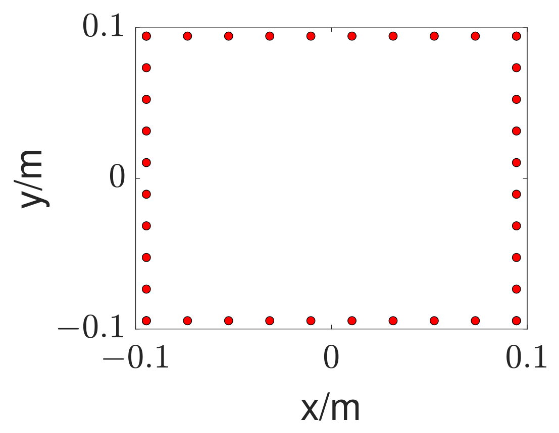
A 36-element equally spaced rectangular array with the element spacing $d_x=d_y=d_{min}=6.58\lambda$ is adopted as the first example. The rectangular array geometry is shown in Figure 3.

According to Equation (16), the positions of the grating lobes are calculated as:

$$\begin{array}{c}\hfill {\xi }_g={\displaystyle \frac{k_{\xi }}{\Delta u}}={\displaystyle \frac{k_{\xi }}{6.58}},{\eta }_g={\displaystyle \frac{k_{\eta }}{\Delta v}}={\displaystyle \frac{k_{\eta }}{6.58}}.\end{array}$$

(26)

Next, the number of elements in the subarray is set to $3\times 3$, i.e., $M=N=3$. The subarray antenna pattern is expressed as:

$$f_{s2}\left(\xi ,\eta \right)=\left({\displaystyle \sum _{m=0}^2}{\displaystyle \sum _{n=0}^2}{e}^{-j{\displaystyle \frac{2\pi }{\lambda }}(m{d}_{\xi }\xi +n{d}_{\eta }\eta )}\right)·f_{n2}\left(\xi ,\eta \right).$$

(27)

To align the nulls of the subarray antenna with the grating lobes of the array, the following equations should be satisfied:

$$\left|{\displaystyle \frac{\sin \left(3\pi d_{\xi }{\xi }_g/\lambda \right)}{\sin \left(\pi d_{\xi }{\xi }_g/\lambda \right)}}\right|=0,\left|{\displaystyle \frac{\sin \left(3\pi d_{\eta }{\eta }_g/\lambda \right)}{\sin \left(\pi d_{\eta }{\eta }_g/\lambda \right)}}\right|=0.$$

(28)

By solving Equation (28), we obtain

$$\begin{array}{c}\hfill d_{\xi }={\displaystyle \frac{d_x}{M}}={\displaystyle \frac{6.58\lambda }{3}}=2.19\lambda ,d_{\eta }={\displaystyle \frac{d_y}{N}}={\displaystyle \frac{6.58\lambda }{3}}=2.19\lambda .\end{array}$$

(29)

At the operating frequency, the derived spacings correspond to $d_{\xi }=d_{\eta }=7.00$ mm and are used as the center-to-center spacings between adjacent small horn elements. For the HFSS model, the aperture dimensions of each small horn are selected as 7 mm × 5.33 mm. This choice ensures a physically realizable $3\times 3$ arrangement while keeping the total aperture of the complete subarray antenna within the minimum element spacing of the sparse array. The resulting total aperture dimensions of the complete subarray antenna are 21 mm × 19.33 mm in the $\eta$ and $\xi$ directions, respectively. For a fair comparison, the conventional rectangular horn antenna is assigned the same aperture dimensions.

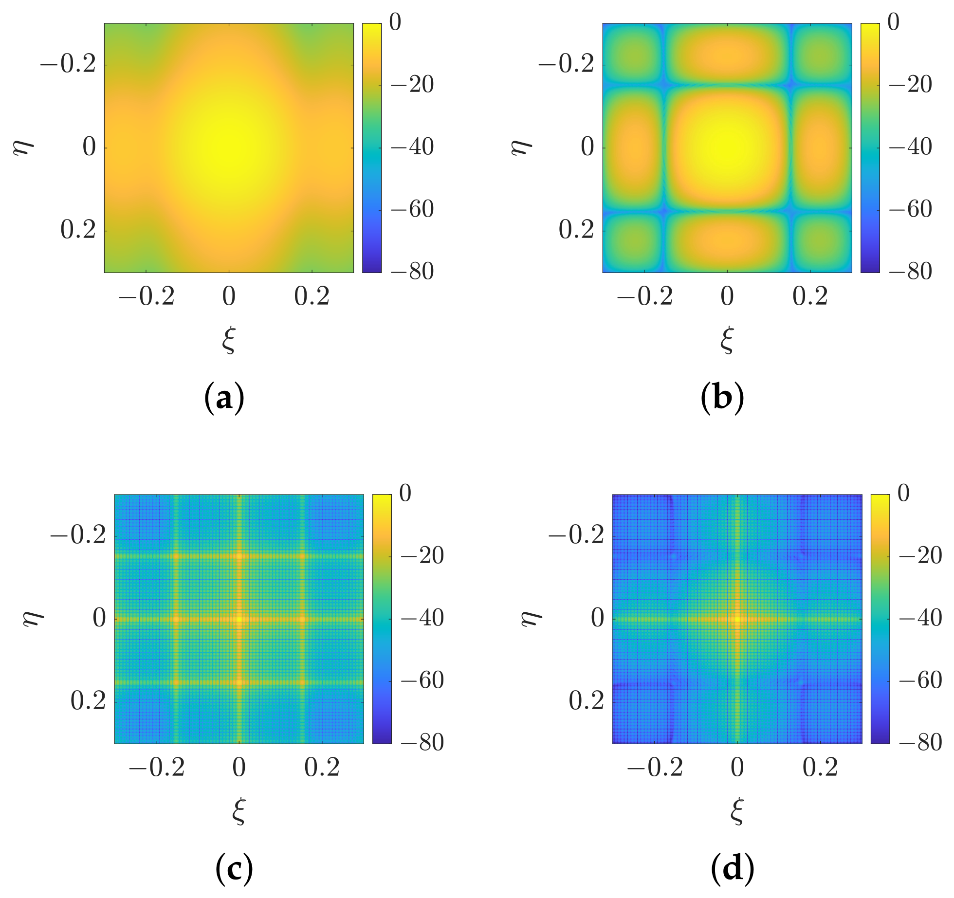
Full-wave electromagnetic simulations of the conventional horn antenna and the subarray-based antenna are then conducted in HFSS. The radiation patterns of the two antennas are shown in Figure 4a,b. By combining the antenna patterns with the corresponding array factors, the resulting array patterns are obtained and illustrated in Figure 4c,d.

As shown in Figure 4, the nulls of the subarray antenna pattern are located near the nearest grating lobe directions, effectively suppressing them.

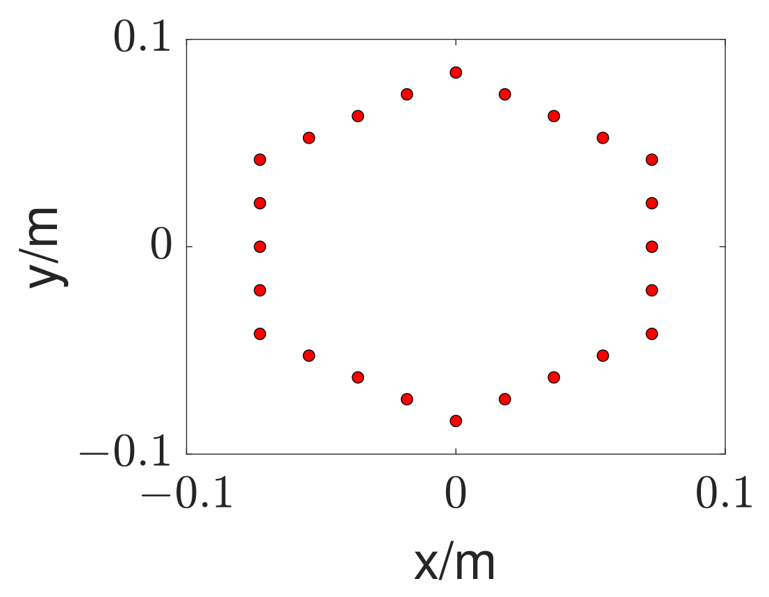
4.1.2. Case 2: A Uniform Hexagonal Array with 24 Elements and $d_{\min }=6.58\lambda$

A 24-element uniform hexagonal array with a minimum element spacing of $d_{\min }=6.58\lambda$ is considered as the second example. Its geometry is shown in Figure 5.

For a source at the FOV center, Equation (16) gives the grating lobe locations as

$$\begin{array}{cc}\hfill {\xi }_g& ={\displaystyle \frac{k_{\xi }}{\Delta u}}={\displaystyle \frac{k_{\xi }}{\left(\sqrt{3}/2\right)d_{\min }/\lambda }}={\displaystyle \frac{k_{\xi }}{5.6984}},{\eta }_g={\displaystyle \frac{k_{\eta }}{\Delta v}}={\displaystyle \frac{k_{\eta }}{d_{\min }/\lambda }}={\displaystyle \frac{k_{\eta }}{6.58}}.\hfill \end{array}$$

(30)

Applying the same design procedure with $M=N=3$ gives

$$\begin{array}{cc}\hfill d_{\xi }& ={\displaystyle \frac{d_x}{M}}={\displaystyle \frac{\left(\sqrt{3}/2\right)d_{\min }}{3}}=1.89\lambda ,d_{\eta }={\displaystyle \frac{d_y}{N}}={\displaystyle \frac{d_{\min }}{3}}=2.19\lambda .\hfill \end{array}$$

(31)

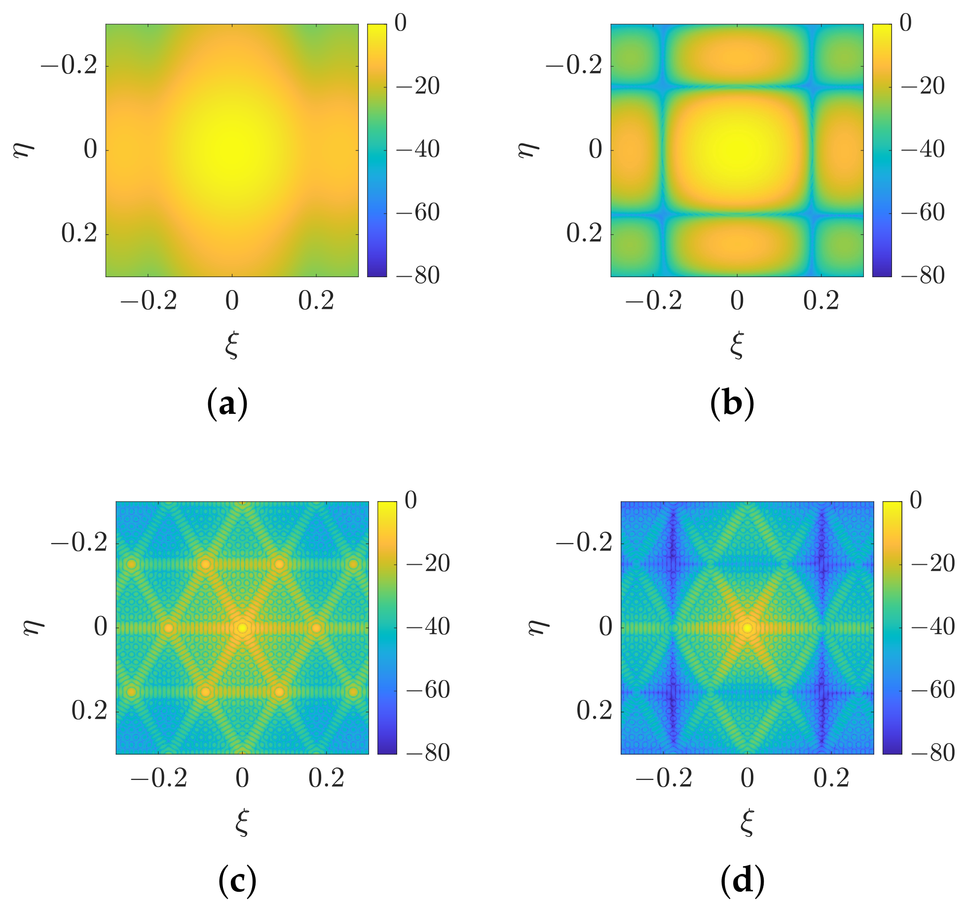
At the operating frequency, these spacings correspond to $d_{\xi }=6.06$ mm and $d_{\eta }=7.00$ mm. The aperture dimensions of each small horn are selected as 7 mm × 5.33 mm, resulting in total aperture dimensions of 21 mm × 17.45 mm in the $\eta$ and $\xi$ directions, respectively. The conventional rectangular horn antenna is assigned the same aperture dimensions. The corresponding HFSS antenna patterns and the resulting array patterns are shown in Figure 6a–d.

As shown in Figure 6, the subarray antenna pattern places nulls near the nearest grating lobe directions, thereby suppressing the corresponding grating lobe responses.

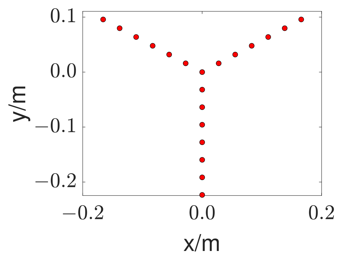
4.1.3. Case 3: A Uniform Y-Shaped Array with 22 Elements and $d_{\min }=10\lambda$

A 22-element uniform Y-shaped array with a minimum element spacing of $d_{\min }=10\lambda$ is considered as the third example. Its geometry is shown in Figure 7.

For a source at the FOV center, Equation (16) gives the grating lobe locations as

$$\begin{array}{cc}\hfill {\xi }_g& ={\displaystyle \frac{k_{\xi }}{\Delta u}}={\displaystyle \frac{k_{\xi }}{\left(\sqrt{3}/2\right)d_{\min }/\lambda }}={\displaystyle \frac{k_{\xi }}{8.6603}},{\eta }_g={\displaystyle \frac{k_{\eta }}{\Delta v}}={\displaystyle \frac{k_{\eta }}{d_{\min }/\lambda }}={\displaystyle \frac{k_{\eta }}{10}}.\hfill \end{array}$$

(32)

Applying the same design procedure with $M=N=3$ gives

$$\begin{array}{cc}\hfill d_{\xi }& ={\displaystyle \frac{d_x}{M}}={\displaystyle \frac{\left(\sqrt{3}/2\right)d_{\min }}{3}}=2.89\lambda ,d_{\eta }={\displaystyle \frac{d_y}{N}}={\displaystyle \frac{d_{\min }}{3}}=3.33\lambda .\hfill \end{array}$$

(33)

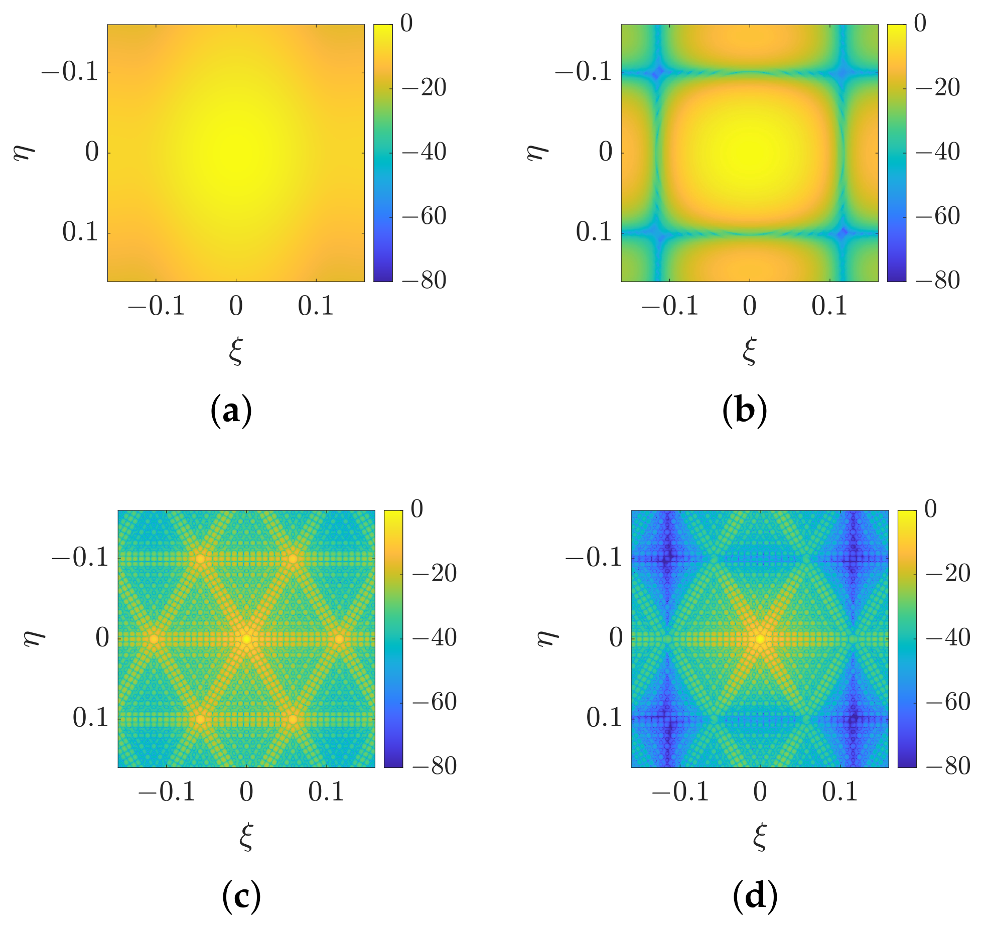
At the operating frequency, these spacings correspond to $d_{\xi }=9.21$ mm and $d_{\eta }=10.64$ mm. The aperture dimensions of each small horn are selected as 10.63 mm × 8.09 mm, resulting in total aperture dimensions of 31.91 mm × 26.51 mm in the $\eta$ and $\xi$ directions, respectively. The conventional rectangular horn antenna is assigned the same aperture dimensions. The corresponding HFSS antenna patterns and the resulting array patterns are shown in Figure 8a–d.

As shown in Figure 8, the subarray antenna pattern places nulls near the nearest grating lobe directions at the FOV center, thereby suppressing the corresponding grating lobe responses.

For clarity and reproducibility,

Table 2. Geometrical parameters of the conventional and subarray-based antenna models used in the HFSS simulations for Cases 1–3.

Case	Antenna Model	Horn Aperture ${\mathit{a}}_{\mathit{\eta }}\times {\mathit{a}}_{\mathit{\xi }}$ (mm)	Phase-Center Spacings ${\mathit{d}}_{\mathit{\eta }},{\mathit{d}}_{\mathit{\xi }}$ (mm)	Overall Aperture ${\mathit{A}}_{\mathit{\eta }}\times {\mathit{A}}_{\mathit{\xi }}$ (mm)
Case 1	conventional	$21.00\times 19.33$	–	$21.00\times 19.33$
	subarray	$7.00\times 5.33$	$7.00,7.00$	$21.00\times 19.33$
Case 2	conventional	$21.00\times 17.45$	–	$21.00\times 17.45$
	subarray	$7.00\times 5.33$	$7.00,6.06$	$21.00\times 17.45$
Case 3	conventional	$31.91\times 26.51$	–	$31.91\times 26.51$
	subarray	$10.63\times 8.09$	$10.63,9.21$	$31.91\times 26.51$

summarizes the geometrical parameters used in the HFSS simulations for Cases 1–3. For the subarray-based antenna, $d_{\eta }$ and $d_{\xi }$ denote the center-to-center spacings between adjacent small horn elements in the $\eta$ and $\xi$ directions, respectively. The horn aperture listed for the conventional antenna represents the aperture of the single horn, whereas that listed for the subarray-based antenna represents the aperture of each small horn element. The overall aperture represents the complete physical aperture of the conventional horn or the complete $3\times 3$ subarray antenna.

In all three cases, the $\eta$ and $\xi$ directions are aligned with the x- and y-axes, respectively. All horn elements have the same orientation, and the aperture center of the conventional horn and that of the central small horn in the subarray are located at the coordinate origin.

4.2. Array Performance Comparison

Based on the previous simulation results, this subsection compares the conventional and subarray-based antenna arrays in terms of angular resolution, sensitivity, and sidelobe level.

4.2.1. Angular Resolution

To assess the impact of the proposed subarray design on both antenna-level and array-level performance,

Table 3. HPBW, angular resolution, and gain comparison between the conventional and subarray-based antenna arrays in Cases 1–3.

Case	Array	HPBW	Angular Resolution	Gain
Case 1	conventional	10.42°	0.55°	24.61 dB
	subarray	7.84°	0.55°	25.72 dB
Case 2	conventional	10.07°	0.79°	24.86 dB
	subarray	8.43°	0.79°	25.85 dB
Case 3	conventional	7.55°	0.40°	26.74 dB
	subarray	5.55°	0.40°	28.56 dB

summarizes the HPBW of the antenna pattern, the angular resolution of the array, and the gain of the antenna pattern for the conventional and subarray-based antenna arrays in Cases 1–3.

As shown in Table 3, the subarray antennas have narrower main lobes and provide higher main beam gain.The angular resolution of the two arrays remains nearly identical, since it is primarily determined by the sparse array layout rather than the element antenna pattern.

4.2.2. Sensitivity

This subsection evaluates the sensitivity performance of the arrays in Case 1 and Case 2 using theoretical calculations and imaging simulations. The simulations assume a uniform TB scene of 323 K, with $T_A=323$ K, $T_R=500$ K, $B=1$ GHz, and $\tau =0.1$ s. In the sensitivity calculation, the 1.2 dB value is treated as an estimated excess insertion loss of the feed network.

Using Case 1 as an example, according to Equations (11) and (13), the theoretical value of the standard deviation of the modified TB is:

$$\Delta T_M=42.33\mathrm{K},$$

(34)

and the theoretical values of the standard deviation of the actual TB at boresight are:

$$\begin{array}{cc}\hfill \Delta T_{con}(0,0)& =2.10\mathrm{K},\hfill \\ \hfill \Delta T_{sub}(0,0)& =1.88\mathrm{K}.\hfill \end{array}$$

(35)

where $\Delta T_M$ denotes the modified TB standard deviation, $\Delta T_{con}$ and $\Delta T_{sub}$ denote the actual TB standard deviation of the conventional array and the subarray-based antenna array at boresight, respectively.

To validate these theoretical results, imaging simulations are conducted, and the Allan standard deviation of each pixel is computed as:

$$\begin{array}{c}\hfill \Delta T_M^{\prime }\left(\xi ,\eta \right)=\sqrt{{\displaystyle \frac{1}{2\left(N-1\right)}}\sum _{i=1}^{N-1}{\left({\widehat{T}}_{i+1}\left(\xi ,\eta \right)-{\widehat{T}}_i\left(\xi ,\eta \right)\right)}^2},\\ \hfill \Delta T^{\prime }\left(\xi ,\eta \right)=\sqrt{{\displaystyle \frac{1}{2\left(N-1\right)}}\sum _{i=1}^{N-1}{\left({\widehat{T}}_{B,i+1}\left(\xi ,\eta \right)-{\widehat{T}}_{B,i}\left(\xi ,\eta \right)\right)}^2},\end{array}$$

(36)

where the number of independent reconstructions N is set to 1000.

According to Equation (36), the standard deviations of the modified TB and the actual TB at boresight are:

$$\begin{array}{cc}\hfill \Delta T_M^{\prime }& =46.48\mathrm{K},\hfill \\ \hfill \Delta T_{con}^{\prime }(0,0)& =2.31\mathrm{K},\hfill \\ \hfill \Delta T_{sub}^{\prime }(0,0)& =2.06\mathrm{K}.\hfill \end{array}$$

(37)

The sensitivities obtained from imaging simulations are slightly higher than the theoretical values, while exhibiting the same distribution and trends.

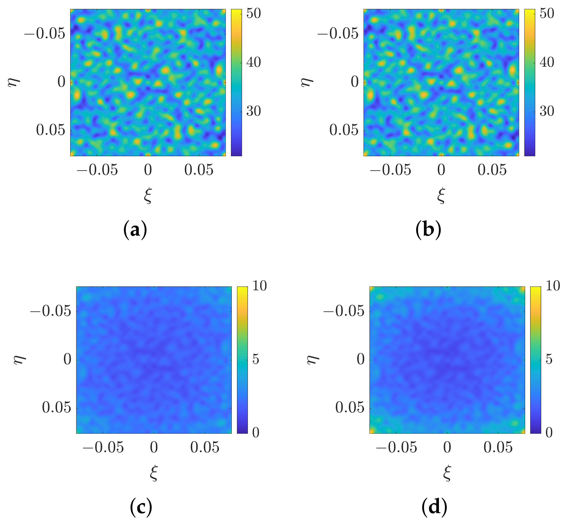
The distributions of the modified TB standard deviation and actual TB standard deviation in Case 1 are shown in Figure 9. The results show that the modified TB standard deviations of the conventional and subarray-based antenna arrays are nearly identical. The actual TB standard deviation of the subarray-based antenna array slightly degrades near the edge of the effective FOV, mainly due to the reduced gain of the subarray antenna pattern in that direction.

To further quantify the impact of the subarray-based antenna on sensitivity performance, we compare the boresight standard deviation and the average standard deviation of reconstructed TB images within the effective FOV.

Table 4. Boresight standard deviation of the reconstructed TB for the conventional and subarray-based arrays in Cases 1 and 2.

Case	Array	$\mathbf{\Delta }{\mathit{T}}_{\mathit{M}}$	$\mathbf{\Delta }\mathit{T}$	$\mathbf{\Delta }{\mathit{T}}_{\mathit{M}}^{\prime }$	$\mathbf{\Delta }{\mathit{T}}^{\prime }$
Case 1	conventional	42.33 K	2.10 K	46.48 K	2.31 K
	subarray	42.33 K	1.88 K	46.48 K	2.06 K
Case 2	conventional	30.63 K	1.52 K	34.00 K	1.74 K
	subarray	30.63 K	1.32 K	34.00 K	1.51 K

and

Table 5. Average standard deviation of the reconstructed TB over the effective FOV for the conventional and subarray-based arrays in Cases 1 and 2.

Case	Array	$\overline{\mathbf{\Delta }{\mathit{T}}_{\mathit{M}}^{\prime }}$	$\overline{\mathbf{\Delta }{\mathit{T}}^{\prime }}$
Case 1	conventional	39.35 K	2.22 K
	subarray	39.35 K	2.74 K
Case 2	conventional	23.20 K	1.74 K
	subarray	23.20 K	2.13 K

list the results for Case 1 and Case 2.

Table 4 and Table 5 show that the modified TB standard deviations of the conventional and subarray-based antenna arrays are nearly identical within the effective FOV. For the actual TB standard deviation, the result becomes direction dependent. At boresight, the subarray-based antenna array achieves a lower actual TB standard deviation than the conventional array. Near the edge of the effective FOV, however, the actual TB standard deviation of the subarray-based antenna array increases. This is mainly because the subarray antenna gain in these directions is lower than that of the conventional antenna.

The influence on detection performance can be quantified using the minimum detectable TB difference. If the detection threshold is defined as $k\Delta T^{\prime }$, where k is a prescribed threshold factor and $\Delta T^{\prime }$ is the actual TB standard deviation, the increase in the minimum detectable actual TB difference is $k\Delta T^{\prime }$. According to Table 5, the average actual TB standard deviation increases from 2.22 K to 2.74 K in Case 1 and from 1.74 K to 2.13 K in Case 2. Therefore, the corresponding increases in the minimum detectable actual TB difference are $0.52k$ K and $0.39k$ K, respectively. For example, if a $3\sigma$ detection threshold is used, the increases are 1.56 K and 1.17 K for Case 1 and Case 2, respectively. These results show that the sensitivity penalty for actual TB retrieval is limited in absolute magnitude, although it should still be considered when accurate quantitative TB retrieval is required. For detection-oriented SAIR applications based on the reconstructed modified TB, the modified TB standard deviation remains nearly unchanged, so the corresponding change in the detection threshold is negligible.

4.2.3. Grating Lobe and Sidelobe Level

As observed from Figure 4, Figure 5, Figure 6, Figure 7 and Figure 8, the nulls of the subarray pattern can be aligned with the grating lobes of the AF, leading to suppression of these grating lobes in the array pattern. The PSLL values of the conventional and subarray-based arrays are very close in all three cases. In Case 1, the PSLL changes from −6.63 dB to −6.78 dB. In Case 2, it changes from −8.33 dB to −8.38 dB. In Case 3, it changes from −7.14 dB to −7.68 dB. The corresponding differences are within 0.54 dB, indicating comparable sidelobe levels.

In summary, aligning the nulls of the subarray antenna pattern with the grating lobe directions effectively suppresses grating lobes while maintaining sidelobe levels comparable to those of the conventional array.

4.3. Imaging Performance Comparison

This subsection compares the imaging performance of the conventional array and the subarray-based array. The simulated arrays and antennas are consistent with the Case 1 configuration. The IDFT method is employed for image reconstruction.

The imaging performance is evaluated under the following scenarios:

• Targets within the effective FOV: The target is within the effective FOV, and the target gradually moves from the center to the edge of the FOV.
• Interference targets: Targets may exist both inside and outside the effective FOV. Targets located outside the effective FOV can be aliased into it, thereby interfering with target detection and localization.

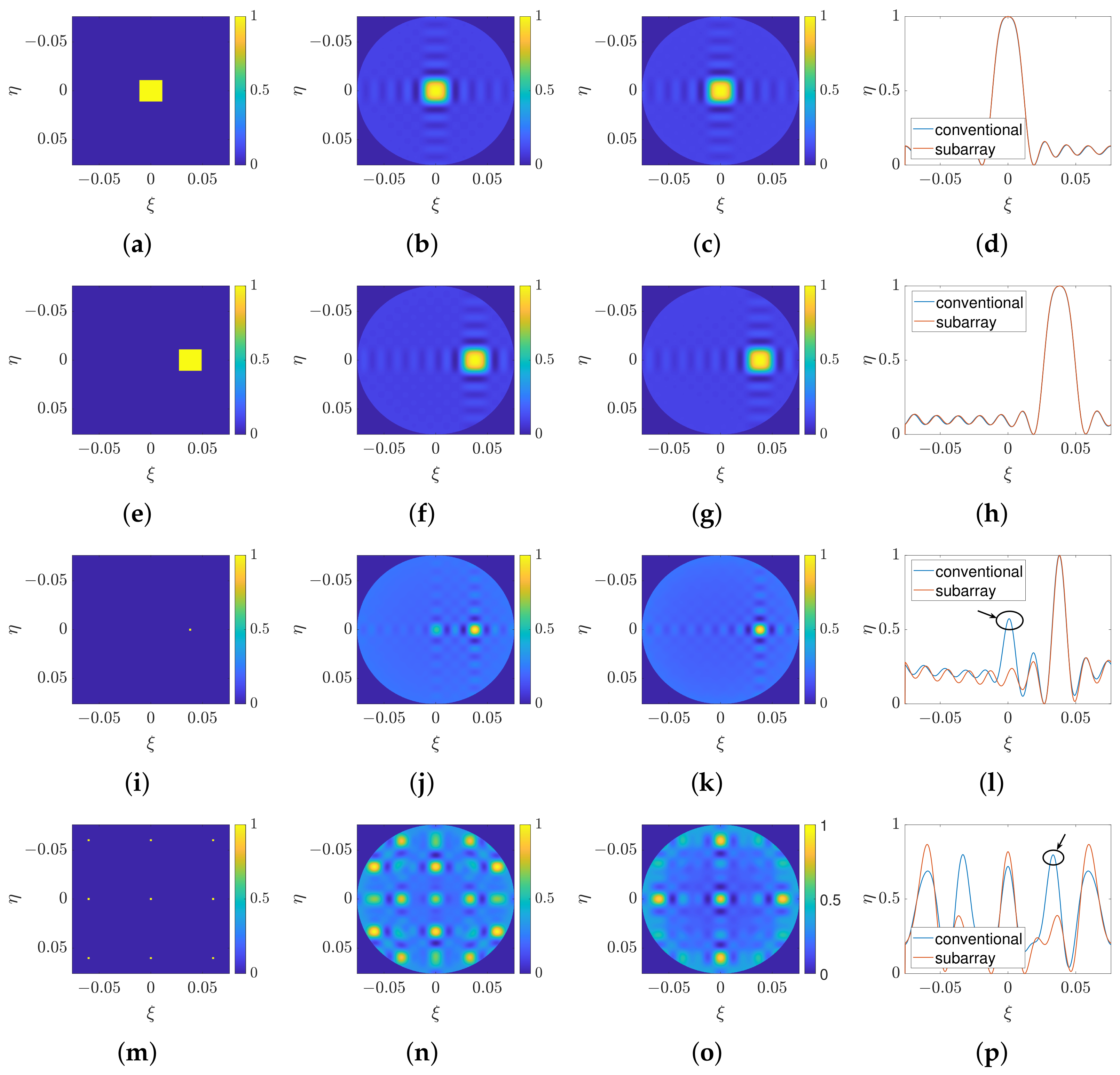
Figure 10 illustrates the imaging results of the conventional array and the subarray array. The actual TB distribution is shown in the first column. The second column shows the imaging results of the conventional array, the third column shows those of the subarray array, and the fourth column shows a cross-sectional comparison of the reconstructed TB images.

As shown in Figure 10a–h, for targets located within the effective FOV, the subarray antenna achieves imaging performance comparable to that of the conventional array. As shown in Figure 10i–p, the imaging results of the conventional array exhibit aliasing artifacts. In contrast, the proposed array effectively suppresses these artifacts, thereby improving the image quality. In the multiple point source scenario, the imaging results of the conventional array show more background noise and stronger artifacts, while the subarray configuration shows a smoother background and clearer target responses.

To further evaluate the imaging performance of the subarray and conventional arrays, the quantitative results for the root mean square error (RMSE), peak signal-to-noise ratio (PSNR), structural similarity index (SSIM), and signal-to-clutter ratio (SCR) [26] are summarized in

Table 6. Comparison of RMSE, PSNR, SSIM, and SCR of the reconstructed TB images obtained with the conventional and subarray-based antenna arrays in Case 1 for targets within the effective FOV (In-FOV targets) and aliased targets.

Metrics	Arrays	In-FOV	In-FOV	Aliased	Aliased
		Target 1	Target 2	Target 1	Target 2
RMSE	subarray	0.1007	0.1038	0.0760	0.2574
	conventional	0.1011	0.1028	0.1860	0.3142
PSNR	subarray	19.9391	19.6874	14.6094	10.5660
	conventional	19.9087	19.7610	13.9810	10.0551
SSIM	subarray	0.9992	0.9991	0.9959	0.9908
	conventional	0.9992	0.9991	0.9953	0.9898
SCR	subarray	22.2865	21.8677	16.2202	5.3113
	conventional	22.1487	21.8089	16.0778	5.0756

.

As shown in Table 6, the RMSE, PSNR, SSIM, and SCR values are very close for the two arrays. For the aliased-target scenarios, the subarray-based array provides lower RMSE and higher PSNR values than the conventional array, which indicates reduced reconstruction error and improved image quality. The SCR metric further characterizes the contrast between the target response and the residual background clutter. The higher SCR values obtained by the subarray-based array in the aliased-target cases indicate improved target-background separability and more effective suppression of residual aliasing artifacts. These quantitative results are consistent with the visual comparison of the reconstructed images.

In summary, the subarray-based array maintains similar imaging performance to the conventional array for targets within the FOV, while offering aliasing artifact suppression in interference scenarios.

4.4. Parametric Analysis

4.4.1. Impact of Subarray Layout

The subarray layout determines the distribution of the pattern nulls and therefore influences grating lobe suppression. To examine this effect, the hexagonal sparse array in Case 2 is considered, whose nearest grating lobes exhibit sixfold angular symmetry. Rectangular and hexagonal subarray layouts are compared under the same total aperture constraint to evaluate their null alignment with the grating lobes and the resulting suppression performance.

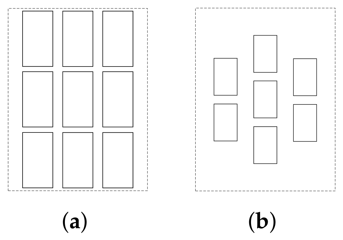
The rectangular subarray layout has been designedin Case 2 in Section 4.1. To design the hexagonal subarray, a seven-element hexagonal subarray consisting of one central element and six surrounding elements is considered, as shown in Figure 11b. Let $d_h$ denote the spacing between adjacent elements in the hexagonal subarray. The coordinates of the seven subarray elements are given by

$$\begin{array}{cc}\hfill & (0,0),(0,d_h),\left({\displaystyle \frac{\sqrt{3}{d}_h}{2}},{\displaystyle \frac{d_h}{2}}\right),\left({\displaystyle \frac{\sqrt{3}{d}_h}{2}},-{\displaystyle \frac{d_h}{2}}\right),\hfill \\ \hfill & (0,-d_h),\left(-{\displaystyle \frac{\sqrt{3}{d}_h}{2}},-{\displaystyle \frac{d_h}{2}}\right),\left(-{\displaystyle \frac{\sqrt{3}{d}_h}{2}},{\displaystyle \frac{d_h}{2}}\right).\hfill \end{array}$$

(38)

Accordingly, the array factor of the hexagonal subarray can be written as

$$A{F}_{\mathrm{hex}}(\xi ,\eta )=1+2\cos \left({\displaystyle \frac{2\pi d_h}{\lambda }}\eta \right)+4\cos \left({\displaystyle \frac{\pi d_h}{\lambda }}\eta \right)\cos \left({\displaystyle \frac{\sqrt{3}\pi d_h}{\lambda }}\xi \right).$$

(39)

For a sparse hexagonal array with the minimum element spacing $d_{\min }$, the nearest grating lobe directions can be expressed as

$$({\xi }_g,{\eta }_g)\in \left\{\left(\pm {\displaystyle \frac{2\lambda }{\sqrt{3}{d}_{\min }}},0\right),\left(\pm {\displaystyle \frac{\lambda }{\sqrt{3}{d}_{\min }}},\pm {\displaystyle \frac{\lambda }{d_{\min }}}\right)\right\}.$$

(40)

Owing to the symmetry of the hexagonal subarray factor, the spacing $d_h$ can be determined by matching the null of $A{F}_{\mathrm{hex}}(\xi ,\eta )$ with one representative nearest grating lobe direction. Taking $({\xi }_g,{\eta }_g)=\left(2\lambda /\left(\sqrt{3}{d}_{\min }\right),0\right)$, Equation (39) becomes

$$A{F}_{\mathrm{hex}}({\xi }_g,{\eta }_g)=3+4\cos \left({\displaystyle \frac{\sqrt{3}\pi d_h}{\lambda }}·{\displaystyle \frac{2\lambda }{\sqrt{3}{d}_{\min }}}\right).$$

(41)

By enforcing $A{F}_{\mathrm{hex}}({\xi }_g,{\eta }_g)=0$, the element spacing of the hexagonal subarray is obtained as

$$d_h={\displaystyle \frac{d_{\min }}{2\pi }}{\cos }^{-1}\left(-{\displaystyle \frac{3}{4}}\right).$$

(42)

Let $a_h\times b_h$ denote the aperture dimensions of each smaller horn element. According to the geometry in Figure 11b, the horizontal and vertical dimensions of the hexagonal subarray are

$$W_h=\sqrt{3}{d}_h+a_h,H_h=2d_h+b_h,$$

(43)

where $W_h$ and $H_h$ denote the overall horizontal and vertical extents of the hexagonal subarray, respectively. For the case considered here, $d_{\min }=6.58\lambda$, giving $d_h=2.533\lambda$, or $8.08\mathrm{mm}$ at 94 GHz. To maintain the same total aperture dimensions as those used in Case 2, the horizontal and vertical extents of the hexagonal subarray are set to $W_h=17.45\mathrm{mm}$ and $H_h=21\mathrm{mm}$, respectively. According to Equation (43), the aperture dimensions of each smaller horn element are therefore determined as $a_h\times b_h=3.46\mathrm{mm}\times 4.84\mathrm{mm}$.

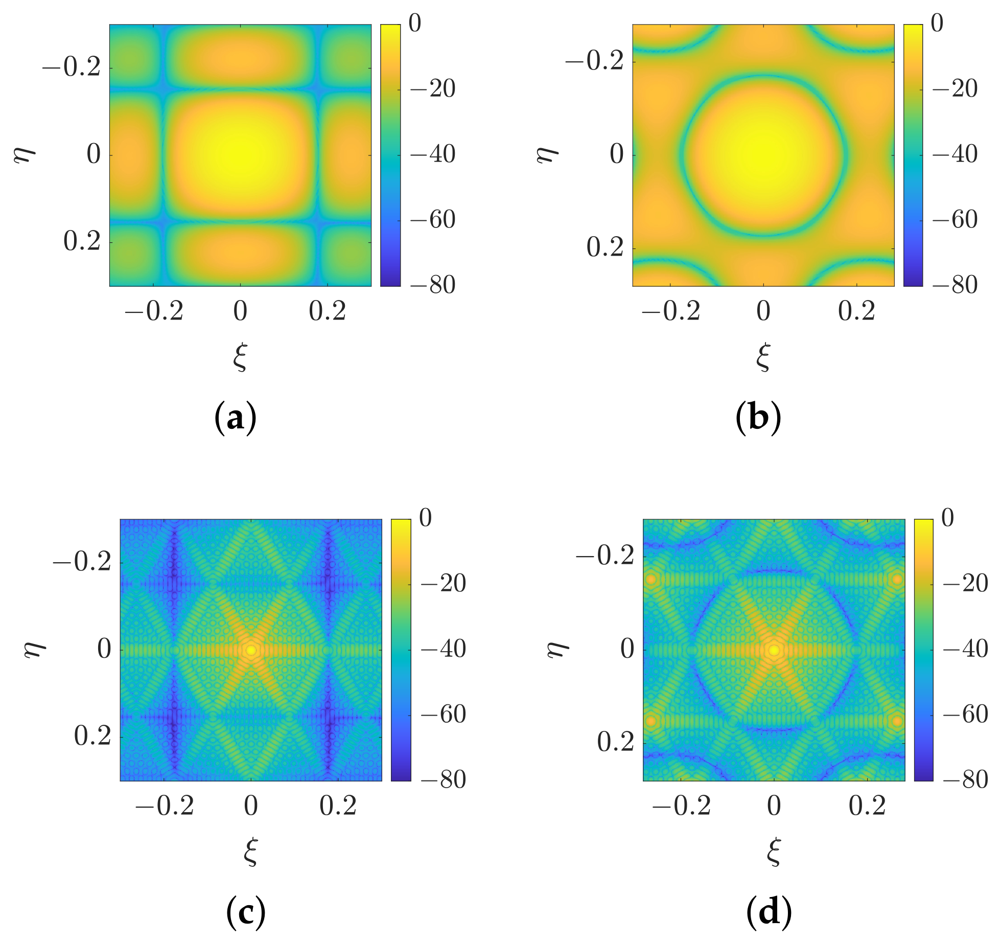
To further compare the practical suppression performance of the two layouts, the simulated antenna patterns and array patterns are shown in Figure 12. Figure 12a,b show the antenna patterns of the rectangular and hexagonal subarrays, while Figure 12c,d present the corresponding array patterns.

As shown in Figure 12, both the rectangular and hexagonal subarrays introduce pattern nulls near the nearest grating lobe directions of the sparse array. The rectangular subarray produces a more regular null distribution, which provides suppression not only at the nearest grating lobe directions but also over a broader set of grating lobe locations, as shown in Figure 12a,c. In comparison, the seven-element hexagonal subarray places its principal nulls near the six nearest grating lobe directions, while the null distribution is less regular at other grating lobe locations, as shown in Figure 12b,d. Therefore, although both layouts suppress the nearest grating lobes, the rectangular subarray provides more consistent suppression over the considered grating lobe distribution. This comparison indicates that the subarray layout should be selected according to the grating lobe distribution of the sparse array and the required suppression range.

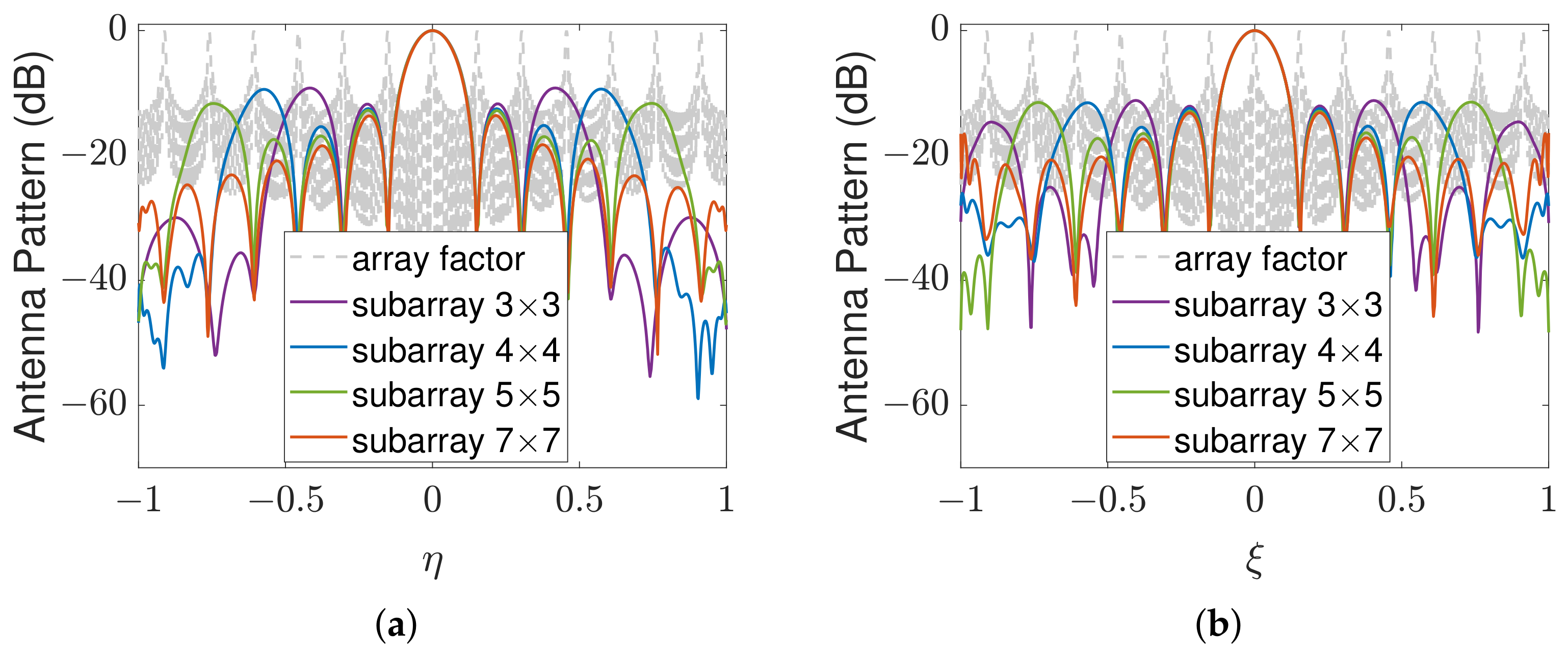
4.4.2. Impact of the Number of Subarray Elements

To examine the effect of the number of subarray elements, the rectangular sparse array in Case 1 is used as a representative example. The total aperture dimensions of the subarray antenna are kept unchanged, while the subarray configuration is varied from $3\times 3$ to $4\times 4$, $5\times 5$, and $7\times 7$. The resulting antenna patterns are shown in Figure 13.

As shown in Figure 13, increasing the number of elements under a fixed total aperture mainly changes the sidelobe characteristics of the subarray antenna pattern, while the main lobe width varies only slightly. The corresponding HPBW, peak sidelobe level (PSLL), and average sidelobe level (ASLL) are summarized in

Table 7. Performance comparison of subarrays with different numbers of elements.

Subarray	HPBW	PSLL	ASLL
$3\times 3$	7.84°	$-9.19$ dB	$-22.87$ dB
$4\times 4$	7.80°	$-9.36$ dB	$-23.00$ dB
$5\times 5$	7.79°	$-11.45$ dB	$-23.36$ dB
$7\times 7$	7.72°	$-13.18$ dB	$-25.13$ dB

.

As the subarray configuration increases from $3\times 3$ to $7\times 7$, the HPBW changes only from 7.84° to 7.72°, indicating that the main lobe width is nearly unchanged under the fixed aperture constraint. In contrast, the PSLL decreases from $-9.19$ dB to $-13.18$ dB, and the ASLL decreases from $-22.87$ dB to $-25.13$ dB. These results show that increasing the number of subarray elements improves the sidelobe characteristics of the antenna pattern without substantially changing its HPBW. The lower sidelobe response can provide additional attenuation at grating lobe directions when the subarray antenna is used in the sparse array.

Therefore, under a fixed total aperture, a larger number of subarray elements provides improved sidelobe control, although it also increases the complexity of the feed network. The number of elements should thus be selected by balancing the required pattern performance and implementation complexity.

4.4.3. Subarray Performance Under Wideband Operation

SAIR systems generally operate over a wide frequency range to improve radiometric sensitivity. Since both the grating lobe locations of the sparse-array AF and the null locations of the subarray AF vary with frequency, their alignment over the operating band should be examined.

Consider a uniformly spaced rectangular array with element spacings $d_x$ and $d_y$ along the x-axis and y-axis, respectively. According to Equation (16), at frequency $f_1$ with wavelength ${\lambda }_1$, the grating lobe locations for a source at the FOV center are

$${\xi }_{g_1}={\displaystyle \frac{k_{\xi }{\lambda }_1}{d_x}},{\eta }_{g_1}={\displaystyle \frac{k_{\eta }{\lambda }_1}{d_y}}.$$

(44)

To suppress the grating lobes at frequency $f_1$, an $M\times N$ subarray is designed with the element spacings

$$d_{{\xi }_1}={\displaystyle \frac{d_x}{M}},d_{{\eta }_1}={\displaystyle \frac{d_y}{N}}.$$

(45)

At a different operating frequency $f_2$, the physical geometry of the subarray remains unchanged. Therefore,

$$d_{{\xi }_2}=d_{{\xi }_1}={\displaystyle \frac{d_x}{M}},d_{{\eta }_2}=d_{{\eta }_1}={\displaystyle \frac{d_y}{N}}.$$

(46)

At frequency $f_2$, the grating lobe locations become

$$\begin{array}{cc}\hfill {\xi }_{g_2}& ={\displaystyle \frac{k_{\xi }}{\Delta u}}={\displaystyle \frac{k_{\xi }}{d_x/{\lambda }_2}},{\eta }_{g_2}={\displaystyle \frac{k_{\eta }}{\Delta v}}={\displaystyle \frac{k_{\eta }}{d_y/{\lambda }_2}}.\hfill \end{array}$$

(47)

Substituting Equations (46) and (47) into the null alignment condition in Equation (19) gives

$$\left|{\displaystyle \frac{\sin \left(M\pi d_{{\xi }_2}{\xi }_{g_2}/{\lambda }_2\right)}{\sin \left(\pi d_{{\xi }_2}{\xi }_{g_2}/{\lambda }_2\right)}}\right|=0,\left|{\displaystyle \frac{\sin \left(N\pi d_{{\eta }_2}{\eta }_{g_2}/{\lambda }_2\right)}{\sin \left(\pi d_{{\eta }_2}{\eta }_{g_2}/{\lambda }_2\right)}}\right|=0.$$

(48)

Therefore, the nulls remain aligned with the corresponding grating lobe locations at frequency $f_2$.

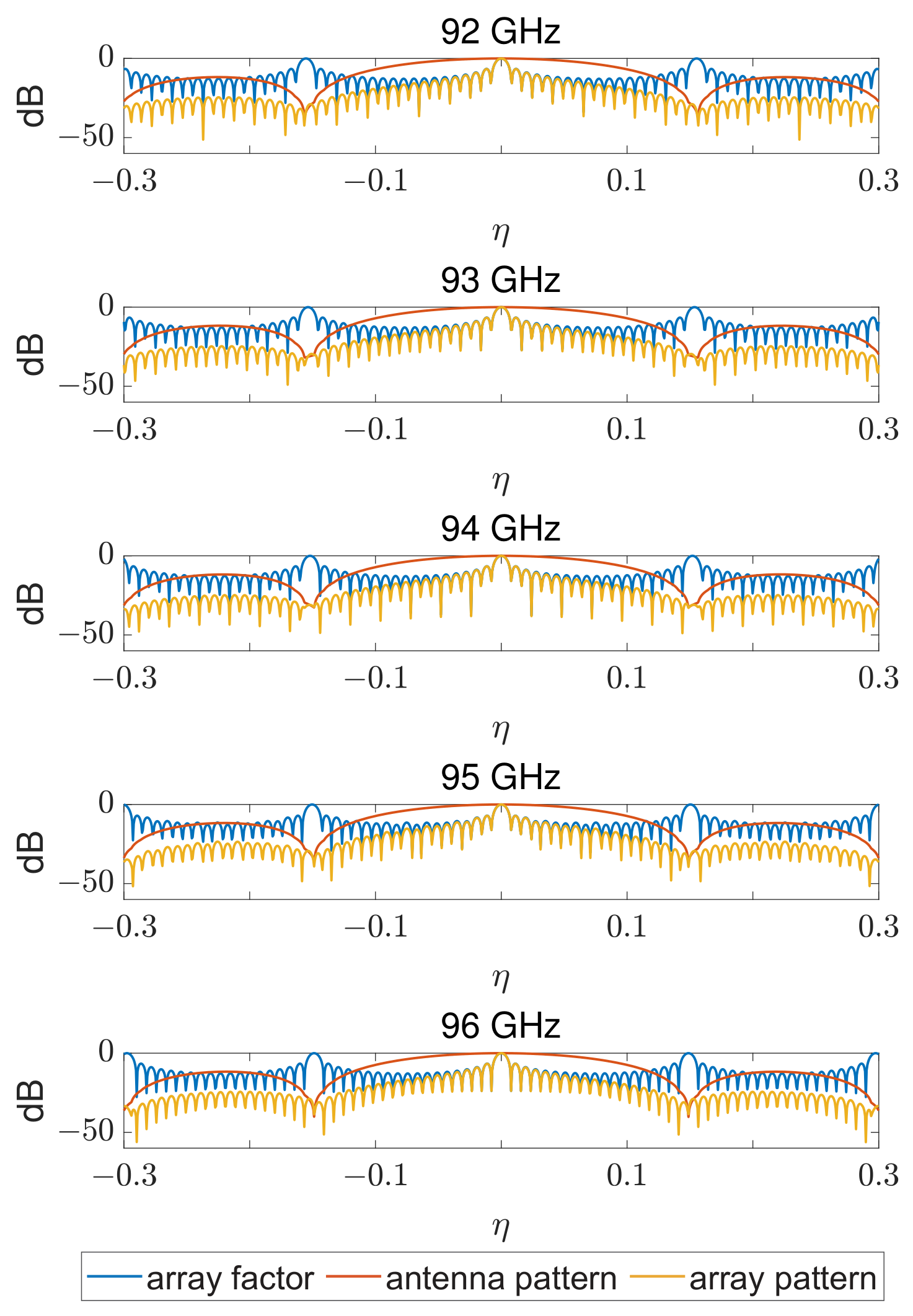
To verify this behavior, the rectangular array in Case 1 is simulated at 92, 93, 94, 95, and 96 GHz. The corresponding subarray antenna patterns, AFs, and overall array patterns are shown in Figure 14. The normalized overall array pattern levels at the nearest grating lobe directions are summarized in

Table 8. Nearest grating lobe levels from 92 to 96 GHz.

Frequency (GHz)	92	93	94	95	96
Nearest Grating lobe level (dB)	$-42.42$	$-40.03$	$-40.35$	$-39.45$	$-40.15$

.

As shown in Figure 14, the subarray pattern nulls remain close to the nearest grating lobe locations over the tested frequency range. The corresponding grating lobe levels remain below $-39$ dB from 92 to 96 GHz, indicating that strong suppression is maintained for the simulated antenna configuration.

The above analysis assumes that the antenna elements and feed network maintain sufficiently stable responses over the operating band. In a fabricated system, frequency dependent insertion loss, amplitude and phase imbalance, element mismatch, and mutual coupling may reduce the realized null depth. These effects should therefore be considered in the wideband feed design and calibration.

4.4.4. Direction Dependence of Grating Lobe Suppression

The preceding design rule is derived for a source at the FOV center. When the source direction changes, the grating lobe locations shift according to Equation (16), whereas the subarray pattern nulls remain fixed by the subarray geometry. The resulting suppression performance is therefore direction dependent. Case 1 is used to evaluate this dependence at the pattern level and its impact on aliasing artifacts in the reconstructed TB images.

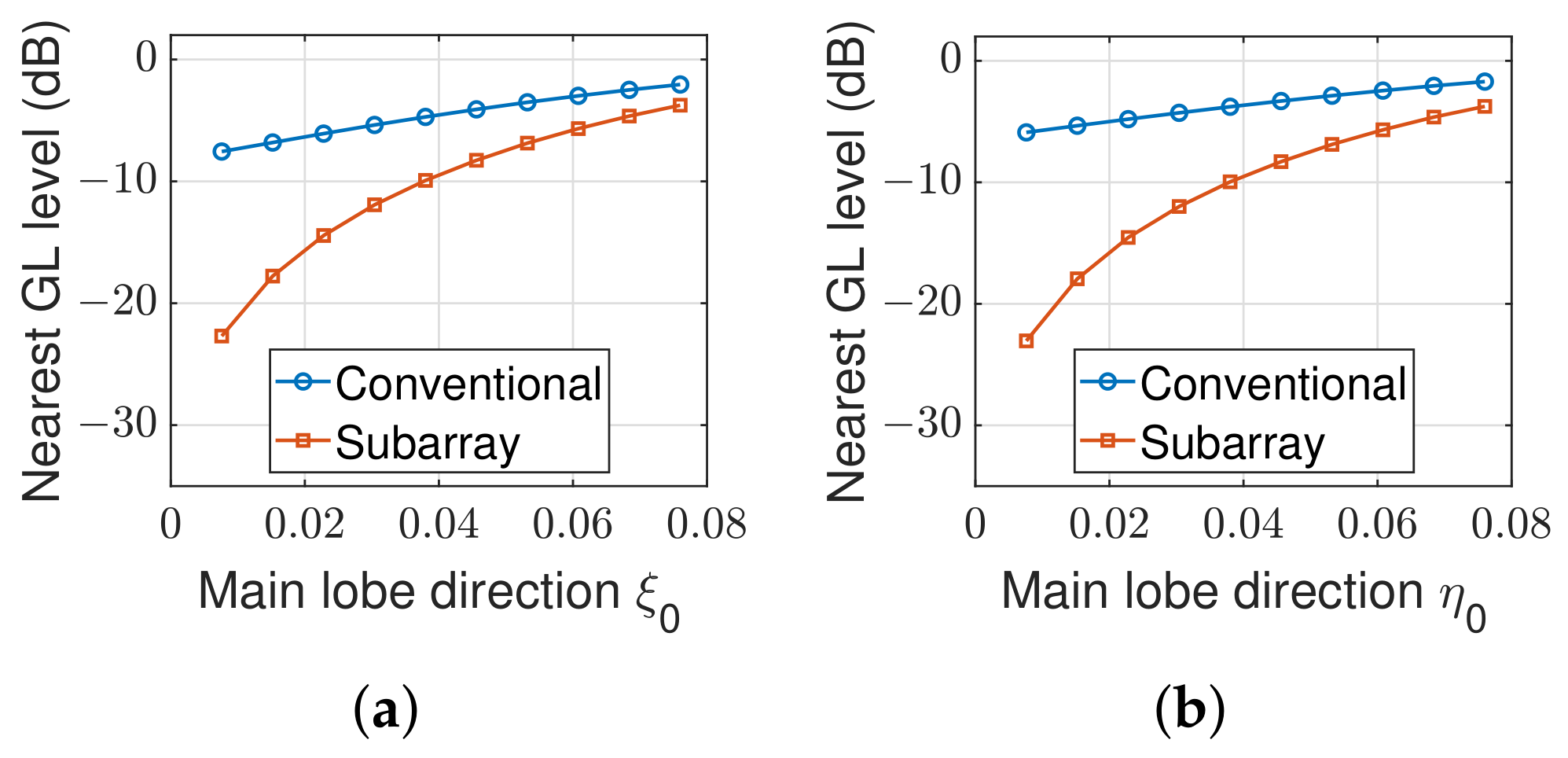
For the pattern level analysis, the source is scanned from the FOV center to the FOV edge along the two coordinate axes. Specifically, ${\eta }_0=0$ and ${\xi }_0\in [0,{\xi }_{\mathrm{FOV}}]$ for the $\xi$-axis scan, while ${\xi }_0=0$ and ${\eta }_0\in [0,{\eta }_{\mathrm{FOV}}]$ for the $\eta$-axis scan, where ${\xi }_{\mathrm{FOV}}=1/(2\Delta u)$ and ${\eta }_{\mathrm{FOV}}=1/(2\Delta v)$. Only the positive half of each axis is considered because of the symmetry.

Let $AP(\xi ,\eta )$ denote the normalized array power pattern. The nearest grating lobe levels for the two scans are defined as

$$\begin{array}{cc}\hfill L_{\xi }\left({\xi }_0\right)& =10{\log }_{10}\left[\underset{k_{\xi }=\pm 1}{\max }AP\left({\xi }_0+{\displaystyle \frac{k_{\xi }}{\Delta u}},0\right)\right],\hfill \\ \hfill L_{\eta }\left({\eta }_0\right)& =10{\log }_{10}\left[\underset{k_{\eta }=\pm 1}{\max }AP\left(0,{\eta }_0+{\displaystyle \frac{k_{\eta }}{\Delta v}}\right)\right].\hfill \end{array}$$

(49)

The nearest grating lobe levels obtained from the two source-direction scans are shown in Figure 15.

As shown in Figure 15, the subarray-based antenna array provides lower nearest grating lobe levels than the conventional antenna array over the examined range. The suppression is strongest near the FOV center and gradually decreases toward the FOV edge. This trend results from the increasing displacement between the shifted grating lobes and the fixed subarray pattern nulls. Consequently, the difference between the two antenna configurations becomes smaller for off-center source directions.

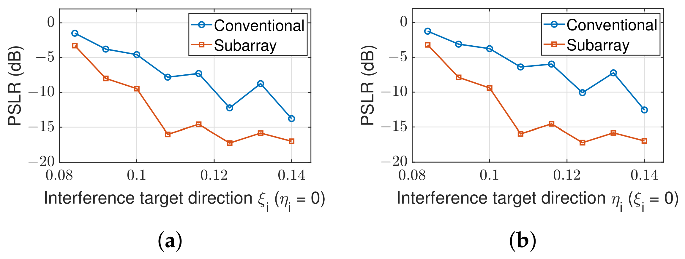
The resulting effect on the reconstructed TB images is evaluated by fixing a target at $({\xi }_t,{\eta }_t)=(0,0)$ and moving an interference source outside the effective FOV. The target and interference source have the same brightness temperature. For the two scans, the interference source is located at $({\xi }_i,0)$ with ${\xi }_i\in [{\xi }_{\mathrm{FOV}},G_{\xi }]$ and at $(0,{\eta }_i)$ with ${\eta }_i\in [{\eta }_{\mathrm{FOV}},G_{\eta }]$, where $G_{\xi }=1/\Delta u$ and $G_{\eta }=1/\Delta v$.

For each interference source direction, the reconstructed TB image is evaluated using the peak sidelobe ratio (PSLR) [27], defined as

$$\mathrm{PSLR}\left(\mathrm{dB}\right)=10{\log }_{10}\left({\displaystyle \frac{I_{\mathrm{artifact}}^{\max }}{I_{\mathrm{target}}^{\mathrm{peak}}}}\right),$$

(50)

where $I_{\mathrm{target}}^{\mathrm{peak}}$ is the reconstructed target peak and $I_{\mathrm{artifact}}^{\max }$ is the maximum sidelobe or aliasing artifact outside the target region. The resulting PSLR values for the two interference-source scans are shown in Figure 16. A lower PSLR indicates stronger artifact suppression.

As shown in Figure 16, the PSLR varies with the interference source direction. The subarray-based antenna array achieves lower PSLR than the conventional antenna array throughout the examined range, with a greater reduction when the interference direction is closer to a designed null region. The exact PSLR values also depend on the target distribution and imaging scene. Therefore, these reconstructed results provide a scene-specific evaluation of the direction dependence rather than a general direction independent bound.

Overall, the proposed spacing rule should be regarded as a nominal design rule for aligning the subarray pattern nulls with the nearest grating lobes under the FOV center condition. As the source or interference direction changes, the null alignment and the resulting suppression depth vary accordingly. Practical implementation should therefore account for both the intended source directions and the specific imaging scenarios.

4.5. Equivalent Experimental Emulation

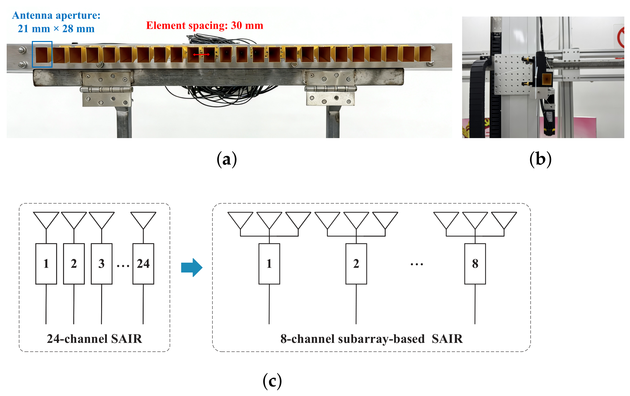
In this subsection, an equivalent experiment based on measured visibility data is presented to evaluate the proposed aliasing suppression method. Since a physical subarray antenna has not yet been fabricated, an existing 24-channel SAIR system is employed to emulate an equivalent 8-channel subarray-based SAIR system. Specifically, three adjacent antenna elements in the original array are grouped to emulate one subarray element according to the designed subarray geometry. The equivalent subarray visibility data are constructed from the measured visibilities of the physical 24-channel SAIR, and the feasibility of this equivalent experiment is theoretically analyzed in Appendix A.

It should be emphasized that the experiment is an equivalent emulation rather than a direct measurement of a fabricated subarray-based antenna. In this experiment, several receiving channels are grouped and combined in post-processing to emulate the effect of a subarray-based receiving element on the measured visibilities and reconstructed TB image. This procedure assumes calibrated channel amplitude and phase responses and negligible radiation pattern mismatch among the grouped elements. Accordingly, the experiment verifies the system-level influence of the proposed subarray concept on SAIR reconstruction, while practical antenna-level effects, such as mutual coupling, feed network loss, and fabrication tolerances, are outside the scope of this emulation and are discussed in Section 5.

The experimental configuration is illustrated in Figure 17. The center frequency of the SAIR system is 94 GHz with a bandwidth of 400 MHz. The original SAIR system consists of 24 receiving elements arranged in a linear array. The aperture size of each rectangular horn antenna is $21\mathrm{mm}\times 28\mathrm{mm}$, and the spacing between adjacent elements is $30\mathrm{mm}$. In the equivalent emulation, every three adjacent antenna channels are grouped as one equivalent subarray-based receiving element, resulting in an equivalent 8-channel subarray SAIR system. The corresponding grouping scheme is shown in Figure 17c. Figure 17a shows the physical layout of the 24-element antenna array, while Figure 17b depicts the noise source used in the experiment. The antenna array and the noise source are located at the same height and separated by 6 m along the horizontal direction. During the measurement, the received signals from all antenna channels are cross-correlated to obtain the measured visibilities. These measured visibility data are subsequently combined according to the grouping scheme shown in Figure 17c to construct the equivalent visibility data of the 8-channel subarray-based SAIR. The TB distributions are then reconstructed using the IDFT.

Two experimental scenarios are considered:

• Targets located within the effective FOV.
• Interference scenario, in which targets are present both inside and outside the effective FOV. Targets located outside the effective FOV may be aliased into the FOV, thereby degrading image quality and target detection.

To verify the effectiveness of the proposed aliasing suppression method, the imaging results of the subarray-based array are compared with those of a conventional antenna array while maintaining identical baseline distributions. Since the subarray-based antenna is realized through an equivalent modeling approach, its effective radiation aperture differs from that of the conventional rectangular horn antenna. Therefore, this experiment focuses exclusively on evaluating the aliasing suppression performance, rather than comparing antenna gain or other radiation characteristics.

Before image reconstruction, the measured visibility samples are calibrated to reduce the influence of receiver gain/phase errors and additive bias terms. Following the standard calibration procedure for SAIRs [28], the calibrated visibility sample is obtained as

$$\tilde{V}={\displaystyle \frac{V_m-V_{\mathrm{bias}}}{V_{\mathrm{cal}}-V_{\mathrm{bias}}}},$$

(51)

where $V_m$ is the measured visibility sample for the point source, $V_{\mathrm{bias}}$ is the bias measurement obtained without the noise source, and $V_{\mathrm{cal}}$ is the calibration measurement obtained with the noise source placed at the boresight. The calibrated visibility samples $\tilde{V}$ are then used in the IDFT method to obtain the TB distribution.

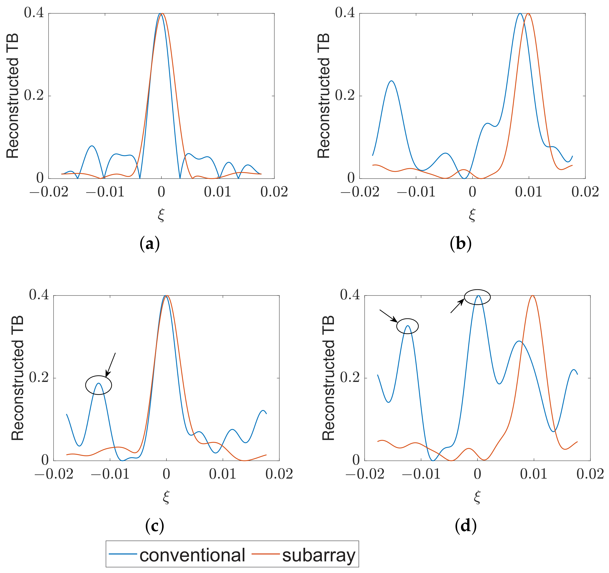
The imaging results for targets within the effective FOV and the interference scenario are shown in Figure 18. Figure 18a,b present the imaging results for targets located within the effective FOV, while Figure 18c,d show the imaging results for the interference scenario, which includes one target inside and one target outside the effective FOV.

To quantitatively evaluate the aliasing suppression capability in the reconstructed TB distributions, the PSLR [27] is analyzed. It is calculated according to Equation (50). The resulting PSLR values for different target scenarios are summarized in

Table 9. Comparison of the peak sidelobe ratio (PSLR) of reconstructed TB distributions obtained with the conventional and subarray-based antenna arrays.

Arrays	In-FOV	In-FOV	Interference	Interference
	Target 1	Target 2	Target 1	Target 2
subarray	−15.61 dB	−12.65 dB	−9.53 dB	−11.27 dB
conventional	−7.03 dB	−2.28 dB	−3.29 dB	2.79 dB

.

As shown in Figure 18a,b, for targets located within the effective FOV, the subarray-based approach yields imaging results with noticeably reduced sidelobe levels compared with the conventional array, indicating improved imaging quality. For the interference scenario shown in Figure 18c,d, the conventional array suffers from pronounced aliasing artifacts within the effective FOV due to the presence of interference targets outside the effective FOV. In contrast, the proposed subarray-based array suppresses these aliasing artifacts, resulting in a cleaner reconstruction of the target within the effective FOV.

Table 9 further provides a quantitative comparison of the PSLR values for different target scenarios. For targets located within the effective FOV, the proposed subarray-based array achieves PSLR values of $-15.61$ dB and $-12.65$ dB for target 1 and target 2, respectively, whereas the conventional array only achieves $-7.03$ dB and $-2.28$ dB. This corresponds to an artifact suppression improvement of approximately $8.58$ dB and $10.37$ dB, respectively. For aliased targets outside the effective FOV, the subarray-based array also provides improved suppression, yielding PSLR values of $-9.53$ dB and $-11.27$ dB compared with $-3.29$ dB and $2.79$ dB obtained with the conventional array. The corresponding improvements reach $6.24$ dB and $14.06$ dB, respectively. These equivalent emulation results support the effectiveness of the proposed subarray-based antenna architecture in suppressing aliasing artifacts under the stated system-level assumptions.

5. Discussion

This section discusses the physical mbechanism of the proposed method, its relation to existing SAIR approaches, and the main practical considerations and limitations.

5.1. Physical Mechanism and Relation to Classical Subarray Theory

According to the pattern multiplication principle, the system response is jointly determined by the AF and the element pattern. Therefore, grating lobe responses can be attenuated by placing nulls of the element pattern near the corresponding grating lobe directions. This mechanism is consistent with the pattern synthesis principle of classical subarray theory. However, its implementation in the proposed SAIR architecture differs from conventional active phased-array. In phased arrays, undesired responses are commonly controlled by adjusting the excitation amplitudes and phases of the array elements, and the resulting performance is mainly evaluated from the radiation pattern. In the proposed architecture, each conventional antenna is replaced by a passive subarray-based antenna with a single output. The signals received by the internal elements are combined before the correlation stage and therefore do not introduce additional channels or correlators. The resulting subarray pattern is fixed by the subarray geometry, element characteristics, and feed network In the SAIR measurement process, this pattern acts as a receiving response that weights the observed TB distribution before correlation. The subarray pattern therefore provides an additional design degree of freedom for suppressing grating lobe responses, and its effectiveness is evaluated through both the overall array pattern and the aliasing artifacts in the reconstructed TB images.

5.2. Comparison with Existing Approaches

Existing aliasing suppression approaches for sparse SAIR systems mainly modify the array configuration, spatial frequency samples, or reconstruction weights. Dense array configurations improve sampling density at the cost of additional antenna elements, receiving channels, and correlators; nonuniform and doubled-FOV array designs modify the distribution of grating lobes or the effective FOV, although they may introduce residual sidelobes, reconstruction complexity, or resolution loss. Interpolation and weighting methods retain the original hardware but may introduce interpolation errors or additional computational burden. In comparison, the proposed method shapes the receiving element pattern to attenuate dominant grating lobe responses without increasing the number of channels or requiring additional reconstruction procedures. Its main implementation requirements are transferred to the passive antenna front end, including subarray design, feed network realization, and calibration.

Table 10. Comparison of representative grating lobe and aliasing suppression approaches for SAIR systems.

Approach	Main Idea	Hardware Requirement	Backend Processing	Main Limitation
Dense array configuration [11]	Uses smaller and more numerous antenna elements to reduce the effective antenna spacing and introduce more short baselines	More antenna elements, receiving channels, and correlators are required	Low	Increased hardware complexity and system cost
Doubled-FOV array design [13]	Enlarges the effective FOV without reducing the minimum antenna spacing	Requires a specific array configuration	Low	Angular resolution loss and degraded imaging performance for extended targets
Nonuniform array design [14,15]	Redistributes grating lobe energy into irregular sidelobes by changing antenna positions	Unchanged	Medium to high	Residual high sidelobes and more complicated reconstruction may remain under strong sparsity
Interpolation-based method [9,16]	Estimates visibility samples to enhance spatial frequency sampling	Unchanged	Medium to high	Interpolation errors may propagate into the reconstructed TB image
Weighting-based method [17]	Suppresses sidelobes by modifying the weighting of measured visibilities	Unchanged	Medium to high	Sidelobe suppression may be accompanied by noise amplification or increased computational cost
Proposed method	Shapes the element antenna pattern to attenuate sparse array grating lobes	Additional subarray antenna and feed network; no additional channels or correlators	Low	Possible feed network loss and imbalance

summarizes these differences.

5.3. Practical Nonidealities and Implementation Considerations

The numerical simulations and equivalent experimental emulation presented in this work are conducted under controlled conditions and therefore do not include all nonidealities of a practical SAIR implementation. The full-wave simulations account for the electromagnetic interactions within each complete subarray antenna, while the practical nonidealities associated with the combining network are not explicitly modeled. The equivalent emulation uses calibrated channels of a one-dimensional SAIR system to reproduce the system-level effect of the proposed subarray concept on measured visibilities and reconstructed TB images, rather than directly characterizing a fabricated subarray antenna. In a practical implementation, frequency dependent feed-network loss, branch amplitude and phase imbalance, fabrication tolerances, element mismatch, and possible coupling between neighboring subarray antennas after integration into the complete sparse array may alter the realized antenna pattern, reduce the null depth, or degrade radiometric sensitivity. These effects should therefore be addressed through feed-network design, calibration, full-array electromagnetic analysis, and fabricated antenna measurements.

5.4. Limitations and Future Work

The proposed spacing rule is derived by aligning the subarray pattern nulls with the nearest grating lobes for a source at the FOV center. Its suppression performance may decrease as the source direction moves away from the designed angular region, as demonstrated by the direction dependence analysis. The rule should therefore be regarded as a nominal design guideline rather than a direction independent suppression rule. In addition, the present study mainly considers representative regular sparse arrays, whereas irregular arrays may exhibit more complicated sidelobe and artifact distributions that cannot be addressed by matching a small number of predetermined null directions. Although the proposed architecture avoids additional receiving channels and correlators, it increases the complexity of the passive antenna front end and its calibration. Future work will therefore investigate joint optimization of the sparse array geometry and element pattern, wider angular and frequency ranges, coupling between neighboring subarray antennas, and fabricated subarray measurements including feed network loss, amplitude and phase imbalance, manufacturing tolerances, and the resulting aliasing suppression performance.

6. Conclusions

This paper proposes an aliasing suppression method for sparse array SAIR systems using a subarray-based antenna architecture. The proposed approach first identifies the grating lobe directions introduced by the sparse array configuration through AF analysis. Then, each conventional antenna element is replaced by a properly designed subarray-based antenna whose pattern introduces nulls aligned with these grating lobe directions, thereby suppressing aliasing artifacts in the reconstructed TB images. Simulation results and equivalent experimental emulation demonstrate that the proposed subarray-based antenna architecture can effectively reduce grating lobe-induced aliasing artifacts while preserving comparable angular resolution and sensitivity. Further analysis evaluates the effects of subarray layout, subarray element number, wideband operation, and source direction on the suppression performance, providing guidance for the application of the proposed design rule in SAIR systems.

Future work will explore more flexible subarray layouts and address practical implementation issues.