


Highlights
What are the main findings?
- An integrated Autonomous Surface Vehicle ASV–drone system enabled high-resolution (centimeter-scale) mapping of chlorophyll-a, turbidity, and fluorescent dissolved organic matter, capturing fine-scale spatial variability not resolved by Sentinel-2 or Landsat imagery.
- Machine learning approaches, particularly Random Forest and ensemble models, outperformed traditional empirical models and demonstrated improved accuracy and generalization across contrasting aquatic environments.
What are the implications of the main findings?
- The integrated monitoring approach provides a flexible and scalable solution for real-time, high-resolution water quality assessment, bridging the gap between point-based sampling and satellite observations.
- The ability to detect fine-scale features such as sediment plumes and near-shore gradients enables more targeted and timely water resource management, including early warning of water quality deterioration and algal blooms.
Abstract
Effective monitoring of inland waters requires approaches capable of capturing high spatial and temporal variability. Traditional in situ sampling provides accurate point measurements but lacks spatial coverage, while satellite remote sensing is often limited by coarse spatial resolution and cloud cover. To address these limitations, this study developed and validated an integrated monitoring platform combining an Autonomous Surface Vehicle (ASV) and a drone-based multispectral imaging system for flexible, high-resolution water quality monitoring. The study was conducted in two contrasting aquatic environments in Alabama: the North River–Lake Tuscaloosa system and the Sardine Pass and Duck Skiff Pass tidal inlets in Mobile Bay. A HyCAT ASV equipped with a YSI EXO2 multiparameter sonde collected continuous in situ measurements of turbidity, chlorophyll-a (Chl-a), and fluorescent dissolved organic matter (fDOM), which served as water-truth for a MicaSense Dual multispectral camera onboard a DJI Inspire-2 drone platform acquiring imagery in 10 spectral bands at ~8 cm spatial resolution. Machine learning models, including ensemble and Random Forest approaches, were developed and compared with traditional empirical algorithms. Ensemble models consistently outperformed empirical approaches, while Random Forest models achieved the highest accuracy and best generalization across variable environmental conditions. Compared with Sentinel-2 and Landsat-8 imagery, the drone-derived maps resolved fine-scale spatial variability, including sediment plumes and near-shore gradients, that could not be detected by satellite sensors. To facilitate operational implementation, the RS-WaterQuality Mapper software tool was expanded to support ensemble and Random Forest analyses for MicaSense imagery. Overall, the integrated ASV–drone system demonstrated substantial advantages over traditional sampling and satellite remote sensing, including rapid deployment, user-controlled acquisition timing, high spatial resolution, and improved monitoring of small and optically complex water bodies, highlighting its potential for adaptive water resource management and early warning applications.
1. Introduction
Inland water bodies, such as rivers, reservoirs, and lakes, are indispensable resources for drinking water supply, irrigation, and ecosystem services. The North River watershed and its primary impoundment, Lake Tuscaloosa in Alabama, exemplify this importance, serving as the primary drinking water source for more than 200,000 people while also supporting extensive recreational activities. However, this system is increasingly stressed by anthropogenic pressures, including urban runoff and agricultural practices, which can result in substantial water quality degradation. The North River has been classified as an impaired water body since 1998, underscoring the urgent need for effective and comprehensive monitoring to support management and restoration efforts [1].
Beyond inland freshwater systems, coastal and estuarine environments are characterized by strong hydrodynamic variability, tidal mixing, and salinity gradients. Mobile Bay, the largest estuary in Alabama and one of the largest estuaries in the United States, was designated an Estuary of National Significance in 1995 under the U.S. Environmental Protection Agency’s National Estuary Program, reflecting its high ecological value and the need for coordinated management of water quality [2,3]. Within the Mobile Bay system, tidal inlets, such as Sardine Pass and Duck Skiff Pass, play a critical role in regulating water exchange between the bay and adjacent coastal waters and represent highly dynamic transition zones between estuarine and coastal environments.
Together, the North River-Lake Tuscaloosa and the Mobile Bay tidal passes represent contrasting yet complementary aquatic environments, spanning freshwater, transitional, and estuarine systems. Studying these sites jointly enables evaluation of remote sensing water quality monitoring approaches across a broad range of optical conditions, hydrological regimes, and anthropogenic influences.
Water quality monitoring is essential, particularly in narrow and highly dynamic aquatic systems, for detecting pollution, managing eutrophication, and providing early warnings of harmful algal blooms. However, such systems are inherently challenging to monitor and often require more sophisticated observation approaches [4,5,6]. Historically, water quality assessment has relied on traditional methods, involving periodic discrete water samples followed by laboratory analysis or stationary sensors from predetermined locations. While providing high-accuracy data for specific points in time and space, field based periodic sampling approach suffers from profound limitations. It is exceptionally labor-intensive, costly, and yields data that is too spatially and temporally sparse to capture fine-scale spatial patterns or the dynamic nature of riverine and lacustrine environments [5,7]. Transient events, such as sediment plumes following a storm or the rapid onset of an algal bloom, are often missed entirely, leading to an incomplete and potentially misleading understanding of the ecosystem’s health.
The advent of satellite-based remote sensing marked a significant advancement, offering the ability to monitor vast areas synoptically and repeatedly. Platforms like Landsat and Copernicus Sentinel-2 series have been instrumental in large-scale water quality studies [8]. However, for the small-to-medium-sized water bodies that constitute most inland water systems, satellite remote sensing faces persistent challenges. The spatial resolution of freely available sensors, such as Sentinel-2 (up to 10–20 m resolution) and Landsat-8 and 9 (up to 30 m resolution), is often too coarse to resolve the fine-scale spatial heterogeneity of these systems. This leads to the problem of mixed pixels, particularly along convoluted shorelines and in narrow river channels, such as, the North River and Mobile Bay Passes where the spectral signature of water is contaminated by that of adjacent land, hence confounding accurate water quality retrieval [6,9]. Furthermore, cloud cover at satellite overpass time can render satellite imagery unusable, and the fixed revisit intervals (e.g., five days for Sentinel-2) are often insufficient to monitor ephemeral water quality events [10].
Autonomous Surface Vehicles (ASVs) and Unmanned Aerial Vehicles (UAVs) (drones) are emerging as transformative tools for high-resolution, flexible water quality monitoring, offering unique advantages that directly address the shortcomings of traditional field and satellite-based approaches [6,11,12,13,14]. ASVs are unmanned boat platforms that can carry water quality sondes and other instruments through difficult-to-access or hazardous waters. They can autonomously navigate pre-programmed routes and continuously log high-fidelity in situ water quality parameters like temperature, dissolved oxygen, algal pigments, and water turbidity. Compared to traditional manned boat surveys, ASVs offer extended endurance, finer spatial coverage, and safer operation in shallow or debris-laden waters. By traversing pre-programmed transects, an ASV can generate dense water quality measurements that overcome the spatial sparseness of fixed monitoring buoys or manned boat discrete point samples. UAVs equipped with multispectral cameras can acquire ultra-high spatial resolution imagery (centimeter-scale) on demand, flying below clouds and targeting specific areas of interest at user-defined temporal frequencies. Drones can thus fill a critical scale gap between point-based sampling and coarse satellite pixels, making them exceptionally well-suited for mapping the fine-scale spatial patterns of optically active water constituents and revealing a level of detail that was previously unattainable.
Previous studies have explored the use of UAVs and autonomous or semi-autonomous aquatic platforms for water quality monitoring. For example, Koparan et al. [15] developed a UAV-based system capable of collecting in situ water quality measurements using onboard sensors and water samplers, while Ryu et al. [16] presented a drone-based real-time water quality monitoring and sampling platform. Other studies have investigated ASVs equipped with water quality sondes for spatially continuous aquatic monitoring. For example, Demetillo et al. [17] developed a low-cost unmanned surface vehicle for real-time water quality monitoring in small aquatic environments, integrating onboard water quality sensors with wireless data transmission. Cryer et al. [18] presented an ASV, equipped with the Chl-a, CDOM, turbidity, and other sensors, to collect high-resolution measurements in shallow coastal environments. However, these studies have primarily focused on either UAV-based sensing/sampling or ASV-based in situ observations independently, rather than integrated workflows that combine synchronous ASV measurements with very high-resolution multispectral drone imaging, machine learning-based retrieval modeling, and operational GIS implementation for water quality mapping across contrasting aquatic environments.
This study aims to demonstrate and validate the capabilities of this integrated autonomous system for high-resolution water quality monitoring that presents an integrated autonomous approach to water quality monitoring in the North River and Mobile Bay Passes using a portable ASV and a drone-based multispectral imaging system. In this research, we deployed and validated an integrated monitoring system comprising a HyCAT ASV (Xylem/YSI Inc., Yellow Springs, OH, USA) equipped with YSI multi-sensor water quality sonde to collect in situ water quality data at high spatial resolution and a DJI Inspire-2 drone (DJI, Shenzhen, China) with a MicaSense Dual camera (MicaSense, Seattle, WA, USA) to acquire simultaneous multispectral imagery. Based on the drone and ASV data, we developed and evaluated machine learning models in comparison with traditional empirical spectral-index algorithms for mapping key water quality parameters, specifically turbidity, chlorophyll-a (Chl-a), and fluorescent dissolved organic matter (fDOM). We demonstrated the superior spatial mapping capabilities of the ASV–drone system through qualitative visual comparisons of its high-resolution outputs with data from traditional sampling and contemporaneous Sentinel-2A and Landsat 8 satellite imagery and highlighted the operational advantages of this flexible, autonomous approach for enabling adaptive and targeted watershed management.
2. Materials and Methods
The overall methodological framework adopted in this study is illustrated in Figure 1. The workflow consists of six major stages: (1) field data acquisition using ASV equipped with a multiparameter water quality sonde and UAV equipped with a multispectral imaging system; (2) UAV image preprocessing to generate radiometrically calibrated reflectance orthomosaics; (3) spatial and temporal matching of in situ water quality measurements with multispectral imagery to construct the modeling dataset; (4) development of empirical, Random Forest, and multipredictor ensemble models for retrieving Chl-a, turbidity, and fDOM; (5) model calibration and independent validation; and (6) application of the best-performing models to generate high-resolution water quality maps. The following subsections describe each stage of the methodology in detail.
Figure 1.
Overall workflow of the proposed multi-platform water quality mapping framework, illustrating field data acquisition, drone image processing, model development, validation, and generation of high-resolution water quality maps.
2.1. Study Area and Field Campaign
The North River is a 72 km long tributary of the Black Warrior River in Alabama and serves as the primary inflow to Lake Tuscaloosa (Figure 2a). The river drains a watershed characterized by mixed agricultural and forested land cover and includes several tributary creeks, with channel widths varying from approximately 30 to 100 m. Water quality in the North River is seasonally influenced by rainfall-driven runoff and temperature, with occasional algal blooms reported during late summer.
Figure 2.
Case study areas and survey designs: (a) North River; (b) Sardine Pass and Duck Skiff Pass.
In 1969, the lower reach of the North River was impounded to form Lake Tuscaloosa, a 24-km2 reservoir with approximately 285 km of shoreline and a storage capacity of about 40 billion gallons. Lake Tuscaloosa exhibits a pronounced longitudinal water quality gradient, with clearer, less productive waters near the dam and increasingly turbid, nutrient-rich conditions in the upstream reaches influenced by riverine inflow. This pronounced spatial heterogeneity along the river–reservoir continuum provides a suitable setting for evaluating high-resolution water quality mapping approaches under varying optical and environmental conditions within a single system.
The second case study area is Duck Skiff Pass and Sardine Pass; two narrow tidal inlets located within the Mobile Bay estuarine system in coastal Alabama (Figure 2b). Duck Skiff Pass is approximately 1 km in length, and Sardine Pass is approximately 0.6 km. These tidal passes are characterized by confined channel geometry and strong hydrodynamic forcing driven by tidal currents, wind, and variable freshwater influence. Water quality conditions within these tidal passes exhibit pronounced spatial and temporal variability associated with tidal mixing, sediment resuspension, and fluctuating salinity gradients. Suspended sediment concentrations and optical water properties can change rapidly over short distances, producing complex conditions distinct from both inland rivers and open estuarine waters. This confined and dynamic setting provides a suitable context for evaluating high-resolution, spatially explicit water quality mapping approaches under highly variable estuarine conditions.
A coordinated field campaign was conducted for each case study site on a single day under clear-sky conditions to ensure consistent illumination and to minimize temporal variability in water quality. The data acquisition platforms and sensors used during the field campaigns are shown in Figure 3, and their key technical specifications are summarized in Table 1.
Figure 3.
Integrated autonomous water quality monitoring system used in this study: (a,b) HyCAT autonomous surface vehicle (ASV); (c) YSI multi-parameter water quality sonde mounted on ASV; (d,e) DJI Inspire 2 unmanned aerial vehicle (UAV); (f) MicaSense Dual multispectral camera mounted on the drone.
Table 1.
Data Acquisition Platforms and Sensors.
For the North River–Lake Tuscaloosa study area, the ASV and UAV surveys were conducted in close succession along an approximately 2.5 km reach of the North River and its mouth region within Lake Tuscaloosa (Figure 2a) on 25 June 2025. The UAV multispectral survey covered approximately 0.48 km2, encompassing the entire ASV survey transect and corresponding in situ water quality measurement locations. Each UAV flight polygon required up to 10 min to complete. In situ water quality measurements were collected immediately before UAV data acquisition, with the time interval between field measurements and the corresponding UAV survey typically not exceeding 10–15 min. Drone flights began at approximately 2:00 PM under clear-sky conditions to optimize illumination geometry and minimize sun-glint effects on the water surface. Satellite observations were also processed to support multi-scale comparison and analysis, including a Sentinel-2C multi-spectral imagery coincident with the field campaign on 25 June 2025 and additional Sentinel-2A multi-spectral imagery on 27 June 2025.
The coordinated field campaign for the Mobile Bay tidal passes was conducted on 2 October 2025 (Figure 2b). In situ water quality measurements using a YSI EXO2 sonde were completed immediately before the UAV survey. Each UAV flight polygon required up to 14 min to complete, and the time interval between in situ measurements and the corresponding UAV data acquisition typically did not exceed 10–15 min. Drone flights began at approximately 1:00 PM under clear-sky conditions. The UAV multispectral survey covered approximately 0.39 km2, encompassing Duck Skiff Pass and Sardine Pass over a combined along-channel distance of approximately 1.6 km together with the corresponding in situ water quality measurement locations. Coincident Landsat-8 satellite overpasses occurred during the field campaign on 2 October 2025, and a Sentinel-2C overpass occurred on 3 October 2025, providing multi-platform observations of the study area for cross-comparison.
2.2. Water Quality Field Data from Autonomous Surface Vehicle
We used a HyCAT Autonomous Surface Vehicle (ASV) (Xylem/YSI Inc., Yellow Springs, OH, USA) to obtain in situ water quality data. The HyCAT is a small (1.8 m length) catamaran ASV designed for remote water monitoring (Figure 3a,b). It is easily portable (≈53 kg) and can be launched from shore without a dock, making it ideal for small rivers. The ASV is battery-powered with an endurance of ~8 h at 2 kts speed, sufficient to cover the study reach in each mission. Its key features include unsinkable foam-filled hulls and a differential thrust steering system powered by two protected pocket thrusters, allowing for high maneuverability. Autonomous navigation and mission planning are managed by an onboard Intel Core i5 computer running HYPACK MAX software v2024 Q2, which uses positioning data from a A222 RTK-compatible GNSS receiver (Hemisphere GNSS, Scottsdale, AZ, USA) to achieve centimeter-level accuracy. The HyCAT was operated in autonomous mode while an onboard GPS provided real-time navigation and data geotagging. A wireless 5.8 GHz link allowed for line-of-sight remote control and data monitoring.
For water quality sensing, the primary in situ sensor payload on HyCAT is a YSI EXO2 multiparameter sonde (Yellow Springs Instruments, Yellow Springs, OH, USA) (Figure 3c), which is seamlessly integrated into one of the vehicle’s hulls. The EXO2 is a state-of-the-art instrument capable of measuring a comprehensive suite of WQPs simultaneously. The EXO2 carried sensors for temperature, conductivity (salinity), pH, dissolved oxygen, turbidity, chlorophyll-a, and fDOM (fluorescent dissolved organic matter) among others. The turbidity sensor is an optical nephelometer (calibrated in NTU), while the chlorophyll-a sensor is a fluorescence probe (excitation/emission for chlorophyll, calibrated to µg L−1 Chl-a). The fDOM sensor (excitation ~365 nm, emission ~450 nm) provides a proxy for CDOM (colored dissolved organic matter) concentration in quinine sulfate units (QSUs). The sensors were calibrated for conductivity, pH, DO, Chl-a, turbidity and fDOM prior to the field survey campaigns with standard solutions, respectively.
During each mission, the ASV continuously logged water quality data at 1 Hz as it traversed the river, producing a dense dataset of georeferenced in situ measurements. Analysis focused on near-surface observations (upper 0.5 m) to align with the effective sensing depth of UAV-based multispectral imagery, which primarily captures reflectance from the water surface and shallow subsurface. In daytime conditions, the North River was generally well mixed, and near-surface measurements were therefore considered representative of bulk water conditions. The ASV navigation path was designed to sample both mid-channel and near-shore zones, enabling characterization of spatial gradients in water quality across the river–reservoir transition. At the Mobile Bay tidal passes, continuous in situ water quality measurements were collected using a manually operated YSI EXO2 sonde due to ASV transportation constraints. Following each field mission, the georeferenced water quality datasets, including latitude, longitude, time, and measured parameters, were retrieved and processed. These in situ measurements were used as reference data for training and validating the remote sensing water quality models.
2.3. Very High-Resolution Imagery from Drone Multispectral Imaging System
The drone platform was a DJI Inspire 2 (Figure 3d,e), a professional-grade quadcopter known for its stability, redundant systems, and powerful flight performance. Its dual-battery system provides a flight time of approximately 23–27 min, and its advanced obstacle avoidance system ensures safe operation over complex environments like river corridors. Mounted on the drone was the MicaSense Dual camera system (MicaSense, Seattle, WA, USA) (Figure 3f).
This advanced sensor payload integrates two cameras to capture imagery in 10 narrow spectral bands. The spectral bands span roughly 440–840 nm, including coastal blue, blue, two green bands, two red bands, three red-edge bands, and a near-infrared (NIR) band. The specific center wavelengths and full-width at half-maximum (FWHM) bandwidths of the bands used in our study were approximately: 444 nm (28 nm), 475 nm (32 nm), 531 nm (14 nm), 560 nm (27 nm), 650 nm (16 nm), 668 nm (14 nm), 705 nm (10 nm), 717 nm (12 nm), 740 nm (18 nm), and 842 nm (57 nm). Each multispectral image has a 1.2 MP resolution per band, yielding a ground sampling distance (GSD) of ~8 cm/pixel at our flight altitude of about 110 m. In addition, the camera captures a co-registered RGB image (at 3.6 MP) for visualization. The MicaSense system includes an upward-facing Downwelling Light Sensor (DLS 2) that logs real-time ambient light and solar angle, and a calibrated reflectance panel (CRP) for on-site radiometric calibration. Together, these components enable precise radiometric correction, converting raw image data into scientifically accurate reflectance values that are comparable across different times and locations.
All flight operations were executed using DJI GS Pro software v.2.0.18, which controlled the Inspire 2 platform, while the MicaSense Dual camera was externally triggered during flight for synchronized multispectral image acquisition. Each survey was flown at 110 m above ground level (AGL) to balance coverage and resolution, achieving a ground sampling distance (GSD) of ~7.5 cm for the multispectral bands. Flights along the river corridor with 40% front overlap and 75% side overlap between images for North River and 75% front overlap and 75% side overlap for Mobile Bay Passes to ensure complete coverage and reliable photogrammetric stitching. The drone’s speed was maintained at ~5 m/s, and the camera was triggered at 1 image per second (nadir oriented) to achieve the desired overlaps. With these settings, each flight covered ~0.5 km of river length per battery (~7 min flight time). Inspire 2’s dual-battery system and high stability allowed safe flights following the sinuous river path even in moderate wind conditions. 23 Ground control points were deployed along North River banks and 10 Ground control points at Sardine Pass bank, their geolocation are measured using differential GPS system. The MicaSense’s built-in GPS geotagging (horizontal accuracy of ~5 m) provided initial georeferencing of the imagery, and then precisely orthorectified with the differential GPS measured GCPs.
After each flight, radiometric calibration of the multispectral imagery was performed using calibrated reflectance panel (CRP) data. Before and after each flight, the UAV hovered and captured images of the reflectance panel under consistent illumination conditions. These panel images, together with downwelling light sensor (DLS) measurements recorded in the image metadata, were used to correct for variable illumination and convert raw digital numbers (DN) to at-surface reflectance.
Initial Drone image processing was conducted using two structure-from-motion photogrammetry software that are widely used for UAV-based remote sensing applications: Pix4D Mapper (Pix4D S.A., Prilly, Switzerland) and Agisoft Metashape Professional (Agisoft LLC, St. Petersburg, Russia). Processing with Pix4D resulted in visible mosaicking artifacts over water surfaces, and therefore Agisoft Metashape Professional was used in this project. The processing workflow consists of several technical steps: (1) importing multispectral drone images (10 spectral images per acquisition, automatically grouped by timestamp); (2) aligning images to generate a three-dimensional point cloud and digital surface model (DSM); (3) applying MicaSense radiometric calibration using the Camera and Sun Irradiance correction, incorporating reflectance panel measurements and downwelling light sensor (DLS) data; and (4) projecting and mosaicking the calibrated reflectance imagery onto the DSM to generate band-specific orthorectified reflectance images (Figure 4).
Figure 4.
True color (RGB) composites of drone multispectral imagery: (a) North River; (b) Sardine Pass and Duck Skiff Pass.
To ensure quality, we visually inspected all drone images, those with motion blur or other distortions were excluded by quality checks. Any obvious sun glint or reflection from the ASV itself was masked out manually. Separate orthomosaics were generated for each of the 10 spectral bands at a spatial resolution of 8 cm, with pixel values representing surface reflectance (0–1.0). Owing to the low flight altitude, atmospheric effects were negligible, and no atmospheric correction was applied to the UAV imagery although rigorous radiometric calibration was performed. The resulting georeferenced reflectance products (WGS84 UTM projection) were subsequently used for spectral extraction at in situ sampling locations and for the computation of spectral indices across the river.
The final reflectance mosaics showed clear delineation of the river channel against the land (vegetation and soil), with minimal image stitching artifacts over water.
2.4. Satellite Data Integration
To investigate multi-scale water quality monitoring and assess algorithm transferability across sensors, satellite imagery was incorporated alongside UAV imagery and in situ water quality observations. For visualization and comparison, the UAV orthomosaics, satellite imagery, and in situ measurement locations were referenced to the same WGS 84 coordinate reference system. For the North River–Lake Tuscaloosa study area, Sentinel-2 imagery from the European Space Agency’s Copernicus program was evaluated. Sentinel-2 carries the MultiSpectral Instrument (MSI), which provides 13 spectral bands at spatial resolutions ranging from 10 to 60 m.
A Sentinel-2C acquisition coincident with the field campaign on 25 June 2025 was heavily affected by cloud cover (>97%) and was therefore unsuitable for comparative analysis. Consequently, a Sentinel-2A Level-1C top-of-atmosphere image acquired on 27 June 2025 with less than 25% scene cloud cover was selected for the comparison analysis. Sentinel-2A imagery was atmospherically corrected to surface reflectance (Level-2A) using the ACOLITE atmospheric correction software v.20250402.0 (Figure 5a). ACOLITE is designed for aquatic remote sensing applications, and its Dark Spectrum Fitting (DSF) algorithm has demonstrated robust performance in optically complex and turbid inland waters by mitigating sun-glint and adjacency effects [19,20].
Figure 5.
True color (RGB) composites of Satellite Multispectral imagery: (a) Sentinel-2A over North River on 27 June 2025; (b) Landsat-8 over Sardine Pass and Duck Skiff Pass on 2 October 2025.
For the Mobile Bay tidal passes, a Landsat 8 multispectral imagery acquired on 2 October 2025 is available, coincident with our UAV flight and in situ survey on the same day. Landsat 8 OLI multispectral imagery contains visible, near-infrared, and shortwave infrared spectral bands at 30 m spatial resolution. The Landsat 8 Level-1 imagery was processed using the same ACOLITE atmospheric correction workflow applied to Sentinel-2, generating remote sensing reflectance (Rrs) products suitable for aquatic and estuarine analysis (Figure 5b). This consistent preprocessing approach facilitated multi-platform interpretation of water quality patterns across the study sites.
2.5. Development of Water Quality Retrieval Models
A matchup dataset was created by spatially and temporally linking the ASV’s in situ measurements with the remotely sensed data. The in situ values were paired with the reflectance values extracted from the corresponding pixels in the drone orthomosaic and the satellite images, forming the basis for model development and validation.
Two classes of models were developed to predict WQPs from the drone’s multispectral reflectance data. This multi-model approach was chosen to scientifically determine the most robust method for this specific environment, rather than assuming a single model fits all conditions.
2.5.1. Spectral Indices and Empirical Models
The empirical models are based on established physical principles of light interaction with water constituents and typically involve spectral indices and combinations of different spectral bands. We focused on the following algorithms previously reported as effective in Case 2 (inland) waters:
- Two-band algorithms (2BDA). Two-band algorithms are among the most widely used empirical approaches for water quality retrieval and are typically based on simple band ratios, differences, or linear combinations of two spectral wavelengths. In inland and estuarine waters, turbidity is primarily driven by suspended particulate matter, which increases backscattering and reflectance in the red and NIR spectral regions. As a result, red-based and red–NIR band combinations have been widely applied for turbidity retrieval, especially under high-turbidity conditions [21,22,23]. In addition, the green band has been shown to be sensitive to suspended solids, while the blue band is comparatively less responsive to changes in turbidity. Consequently, green–blue band ratios have been commonly used as predictors of turbidity [24,25].
For chlorophyll-a (Chl-a), many studies exploit the strong absorption of chlorophyll in the red region and the reflectance peak in the near-infrared (NIR) or red-edge region. A classic example is Gitelson’s two-band algorithm, originally developed for turbid and productive waters, which uses red and NIR (or red-edge) bands to estimate Chl-a concentration through a linear relationship after accounting for baseline scattering effects [26,27,28]. In addition to red–NIR formulations, alternative two-band combinations have been reported for Chl-a estimation, including blue–green and red–green ratios, particularly in optically complex inland and estuarine waters [29,30].
Two-band formulations were further examined for fDOM estimation. fDOM and CDOM primarily influence absorption in the blue portion of the visible spectrum, resulting in reduced blue reflectance relative to longer wavelengths. Accordingly, blue-green and blue-red band ratios have been widely used to estimate fDOM or CDOM concentrations in inland and coastal waters [31,32,33].
- 2.
- Three-band algorithms (3BDA). Three-band algorithms were evaluated as an extension of single- and two-band approaches for retrieving chlorophyll-a (Chl-a). These algorithms combine reflectance from three spectral bands to improve sensitivity to Chl-a under optically complex conditions.
A widely used three-band chlorophyll formulation was proposed by Dall’Olmo and Gitelson, specifically for turbid and productive waters, and exploits strong chlorophyll absorption in the red region while using red-edge and longer-wavelength bands to enhance robustness in the presence of background scattering effects [27]. Additional three-band chlorophyll formulations combining red and red-edge bands have also been reported for multispectral sensors [34,35]. Three-band approaches using blue and green wavelengths have also been applied for Chl-a estimation in estuarine and freshwater environments, particularly where blue reflectance retains sensitivity to chlorophyll variability [36].
- 3.
- Normalized Difference Chlorophyll Index (NDCI) and Normalized Difference Turbidity Index (NTDI). The Normalized Difference Chlorophyll Index (NDCI) is a widely used spectral index developed for chlorophyll-a (Chl-a) retrieval in turbid and productive aquatic environments. NDCI leverages the contrast between strong chlorophyll absorption in the red portion of the spectrum and increased reflectance at longer wavelengths, providing improved sensitivity to chlorophyll variations under optically complex conditions. Previous studies have demonstrated that NDCI performs well in eutrophic waters and often outperforms vegetation-based indices when applied to aquatic systems [37]. Similarly, the Normalized Difference Turbidity Index (NDTI) was calculated as an analogue to NDCI but using red and green bands to enhance sensitivity to suspended sediments [23]. This formulation is based on the tendency for reflectance in the red band to increase with particle scattering, while the green band responds differently under varying sediment loads, making NDTI a commonly used proxy for turbidity in inland and estuarine waters.
- 4.
- Other spectral indices. Several additional spectral indices were calculated to provide complementary information on water optical properties and surface conditions. These indices were included to examine their potential utility in characterizing turbidity, dissolved organic matter, and surface algal features under the observed environmental conditions.
The Surface Algal Bloom Index (SABI) was computed to highlight areas of elevated algal biomass at or near the water surface. SABI combines red and/or longer-wavelength bands with blue–green wavelengths to enhance the spectral signature of dense algal accumulations relative to surrounding waters [38].
We also evaluated the Cyanobacteria Index (CI), which is designed to detect cyanobacterial dominance and surface accumulations based on spectral curvature between the red and red-edge/near-infrared region (~709 nm). However, CI is primarily sensitive to moderate-to-high biomass conditions and dense surface blooms in relatively calm waters. In our analysis, CI as defined by Wynne et al., 2008 for MERIS [39] was computed but did not exhibit a strong or consistent signal, likely because chlorophyll-a concentrations in the North River system were low and concentrations in the Mobile Bay tidal passes, while occasionally exceeding ~10 µg L−1, remained below levels typically associated with cyanobacterial surface scum formation during the survey periods.
From the drone reflectance mosaics, we extracted band values for each parameter’s training and validation dataset. Reflectance values (for all relevant bands) were then used to compute the water quality indices. We performed linear regression of each index against the measured in situ values of Chl-a (µg L−1), turbidity (NTU), and fDOM (QSU). The best-performing index for each water quality parameter was selected for comparison with the ML models.
2.5.2. Machine Learning Models
In addition to spectral index based empirical regression models, we implemented two types of machine learning (ML) models to estimate and map water quality parameters from UAV multispectral imagery.
- Random Forest (RF) model. RF model was applied as a non-parametric machine learning approach for modeling potentially non-linear relationships between UAV-derived spectral indices and water quality parameters. RF constructs multiple decision trees using bootstrap resampling of the training data and aggregates their predictions to improve model robustness and generalization [40,41]. Random Forest has been successfully applied in previous studies to estimate water quality parameters in optically complex inland waters, demonstrating strong performance under non-linear reflectance–concentration relationships [42].
In this study, RF models were trained using 250 regression trees and bootstrap sampling, with a minimum leaf size of 1–15 samples and 2–30 minimum samples to split. All predictor variables were considered at each split, and input predictors were standardized using z-scores based on the training data prior to model fitting.
- 2.
- Multi-predictor Ensemble Model. In addition to Random Forest model, a multi-predictor ensemble learning model was implemented to improve the robustness and generalization of water quality retrieval across optically variable conditions. The ensemble learning model follows the selection-based framework proposed by Xu et al. [35], in which multiple candidate empirical models are jointly to form a model base. These empirical models derived from different spectral indices (e.g., two-band, three-band, normalized difference, and band-ratio formulations) are first calibrated independently using the available training data. These component models together cover and represent various optical and environmental conditions related to phytoplankton absorption, scattering, and background water constituents.
The ensemble employs a spectral-space partitioning strategy, in which the most appropriate component model is dynamically selected for prediction based on the spectral characteristics of each observation. This selection is implemented using a supervised decision tree classifier trained in spectral feature space, allowing different empirical models to be preferentially applied under distinct optical regimes [35].
In this study, the decision tree classifier used for ensemble model selection was trained with a minimum of 10–40 samples per terminal node and a maximum tree depth 3, providing a balance between model flexibility and overfitting control.
The component models of ensemble learning approach are the same as those spectral indices based empirical models, enabling direct comparison between individual empirical models and their ensemble-based integration.
2.5.3. Model Implementation and Evaluation
Separate models were developed and evaluated for each target water quality parameter, including turbidity, chlorophyll-a (Chl-a), and fluorescent dissolved organic matter (fDOM). Prior to model development, paired spectral reflectance and in situ water quality datasets were screened for statistical outliers using a three-standard-deviation (3σ) criterion, as well as residual, leverage, and Cook’s distance diagnostics. The cleaned datasets were then randomly divided into calibration (training) and validation subsets, with 75% of the samples used for model calibration and 25% reserved for independent validation (North River: 327 training points and 109 validation points; Sardine Pass and Duck Skiff Pass: 501 training points and 167 validation points). All model tuning and calibration procedures were performed exclusively on the training data to prevent information leakage, and model performance was assessed using the independent validation dataset.
Model performance was evaluated using the coefficient of determination (R2), Root Mean Square Error (RMSE) and Mean Absolute Error (MAE). These metrics were computed consistently across empirical and machine-learning approaches to enable direct comparison of model performance.
In addition to separate modeling for each study area, the machine-learning models were also trained and evaluated using a combined dataset from both the North River–Lake Tuscaloosa system and the Mobile Bay tidal passes. The combined dataset included 1104 observations, with 828 samples used for model training and 276 samples reserved for validation. With this combined-dataset, we examined model behavior across a broader range of optical conditions and hydrodynamic environments, while maintaining the same training–validation framework and performance metrics.
To operationalize model development, validation, and spatial application, we enhanced a previously developed QGIS-based water quality software tool [43] in order to support the analyses conducted in this study. The tool provided an integrated environment for model training, validation, and raster-based application of empirical, Random Forest, and ensemble models [43]. Our enhancements to the QGIS-based water quality tool include to add the support for the MicaSense Dual sensor; incorporate additional spectral indices for drone data on analogies with Sentinel-2 and Landsat 8/9 formulations, refine ISODATA clustering and decision tree training rules for ensemble learning model, implement predictor normalization for Random Forest and ensemble modeling, extend Random Forest models to support multi-feature (multi-index) inputs; and develop point-based validation tools for both Random Forest and ensemble models.
3. Results
3.1. In Situ Water Quality Conditions
The in situ data collected by the HyCAT ASV and YSI EXO2 provided a high-resolution characterization of surface water quality conditions in the Lake Tuscaloosa system and the Mobile Bay tidal passes during the field campaigns. Descriptive statistics of the measured parameters are summarized in Table 2.
Table 2.
Descriptive Statistics of In Situ Water Quality Parameters.
In the North River system, turbidity varied between 5.33 and 19.51 NTU, reflecting relatively clear baseflow conditions in the area close to main reservoir (Lake Tuscaloosa). Chlorophyll-a concentrations ranged from 1.03 to 9.16 µg L−1, indicating generally low to moderate phytoplankton biomass. CDOM (measured as fDOM in QSU) ranged from 16.32 to 23.57 QSU, with higher values observed in upstream and forest-influenced reaches and slightly lower values in the area close to main reservoir. Dissolved oxygen remained relatively stable (6.99–8.54 mg L−1), and pH ranged between 6.32 and 6.81, indicating mildly acidic to neutral conditions typical of southeastern U.S. reservoirs. Specific conductivity was low (56.60–72.31 µS cm−1), consistent with freshwater conditions.
In contrast, the Mobile Bay passes exhibited more saline estuarine conditions. Specific conductivity values were markedly higher (2118–10,571 µS cm−1), reflecting tidal exchange with saline coastal waters. Turbidity ranged from 5.80 to 24.37 NTU that aligns with North River system, while chlorophyll-a concentrations were substantially higher, ranging from 3.97 to 24.65 µg L−1. CDOM (fDOM) levels were also elevated (32.71–39.47 QSU), reflecting strong terrestrial and estuarine organic matter inputs. Dissolved oxygen ranged from 6.51 to 10.01 mg L−1, and pH was moderately alkaline (7.33–8.08).
The observed variability in turbidity, chlorophyll-a, and fDOM across both systems provided a suitable gradient for remote sensing model development, enabling evaluation of retrieval algorithms under differing optical regimes dominated by phytoplankton, suspended sediments, and dissolved organic matter.
Because turbidity, chlorophyll-a, and fDOM exhibited skewed distributions and deviated from normality, these variables were log10-transformed prior to model development. The log transformation reduced heteroscedasticity and improved linear model stability.
3.2. Comparative Performance of Water Quality Retrieval Models
The performance of the empirical and machine learning models was evaluated using the independent validation dataset. The results, summarized in Table 3, clearly demonstrate the superior predictive power of the machine learning approaches over the traditional empirical algorithms for all three water quality parameters (WQPs).
Table 3.
Performance Evaluation of Empirical and Machine Learning.
Correlation analysis between spectral predictors and water quality parameters identified several candidate empirical relationships. Subsequent evaluation using empirical, ensemble, and Random Forest approaches demonstrated varying predictive performance across sites (Figure 6 and Figure 7). The final best-performing models and spectral predictors differed among water quality parameters and environments.
Figure 6.
Model validation by comparing chlorophyll-a, turbidity, and fDOM predicted by empirical, ensemble, and Random Forest models against field observations for North River.
Figure 7.
Model validation by comparing chlorophyll-a, turbidity, and fDOM predicted by empirical, ensemble, and Random Forest models against field observations for Mobile Bay Passes.
For turbidity, the strongest empirical relationships were obtained using for North River and for Sardine and Duck Skiff Passes. Ensemble turbidity models combined the best-performing turbidity-related spectral indices, including and , whereas Random Forest models incorporated additional spectral predictors, including (red/blue ratio) and (green/blue ratio), resulting in the highest predictive performance across both study areas.
For Chl-a, the best empirical predictors were for North River and for Sardine and Duck Skiff Passes. Ensemble Chl-a models combined the strongest chlorophyll-related spectral indices, including , , , , and , whereas Random Forest models integrated these spectral predictors, producing improved predictive performance across both study areas.
For fDOM, the strongest empirical relationships were obtained using for North River and for Sardine and Duck Skiff Passes. Ensemble fDOM models combined green-red and green-blue spectral indices, including , , and , whereas Random Forest models incorporated these complementary spectral relationships, resulting in improved predictive performance across both study areas.
Turbidity was the most consistently retrievable parameter, particularly in the Mobile Bay passes, where the empirical, ensemble, and Random Forest models achieved R2 values of 0.838, 0.847, and 0.897, respectively. Performance was lower in North River, with corresponding R2 values of 0.509, 0.603, and 0.702. The stronger performance in the estuarine environment may reflect more pronounced sediment-driven spectral signals. When observations from both study areas were combined, the Random Forest turbidity model achieved the highest overall performance (R2 = 0.981; RMSE = 0.019 in log10 units), indicating that nonlinear modeling using a broader range of freshwater and estuarine conditions improved the representation of turbidity-related spectral variability. This finding suggests that turbidity retrieval particularly benefits from machine-learning approaches because the optical response associated with turbidity is influenced not only by suspended sediments but also by concurrent variations in phytoplankton and dissolved organic matter, resulting in complex nonlinear spectral relationships.
Chlorophyll-a was more challenging to retrieve across both environments. Empirical and ensemble models produced similar moderate performance, with R2 values ranging from 0.546 to 0.571. The modest improvement achieved by the ensemble approach suggests that spectral-space partitioning provided some benefit across varying optical regimes, although it was insufficient to fully capture the complexity of chlorophyll-related spectral variability. The study-area-specific Random Forest models provided further improvements (R2 = 0.586 for North River and 0.636 for the Mobile Bay passes). The combined-dataset Random Forest model performed substantially better, explaining approximately 88% of the validation variance, although its RMSE remained higher than those of the study-area-specific models because the combined dataset encompassed a substantially broader chlorophyll-a range and contrasting optical environments. These results indicate that chlorophyll-a retrieval benefited from nonlinear modeling and more environmentally diverse training data but remained sensitive to optical heterogeneity.
fDOM exhibited the strongest contrast in model performance between the two study areas. In North River, empirical, ensemble, and Random Forest models achieved R2 values of 0.703, 0.710, and 0.810, respectively. In the Mobile Bay passes, performance was lower, particularly for the empirical model (R2 = 0.375), while ensemble and Random Forest models improved the R2 to 0.525 and 0.534. The lower estuarine performance may be associated with the relatively narrow fDOM range and the complex mixing of terrestrial and marine dissolved organic matter. Nevertheless, the combined-dataset Random Forest model achieved strong overall performance (R2 = 0.931), suggesting that inclusion of contrasting freshwater and estuarine observations improved the model’s ability to represent fDOM variability across broader optical conditions.
Taken together, these results show that no single empirical relationship adequately captured variability across all optical conditions. The optimal spectral relationships differed between North River and the Mobile Bay passes, demonstrating the limited transferability of study-area-specific empirical models across contrasting aquatic systems. For example, chlorophyll retrieval relationships differed between sites, potentially reflecting shifts in phytoplankton community composition (e.g., differences in pigment packaging or dominance of distinct taxa) that influence reflectance spectra. This observation is consistent with previous findings that a single empirical model often cannot reproduce spatial and temporal variability in dynamic aquatic systems. Empirical indices nevertheless provided useful baseline models and remain valuable for rapid mapping applications where extensive training data are unavailable, whereas Random Forest was better able to incorporate multiple spectral relationships and accommodate nonlinear variability. The improved performance of the combined-dataset Random Forest models further highlights the importance of environmentally diverse training observations for developing models that are applicable across contrasting freshwater and estuarine conditions.
Cross-site application of study-area-specific models revealed reduced performance when applied outside their calibration domain, reinforcing that spatial transferability remains a key challenge in aquatic remote sensing. However, Random Forest models trained on the combined dataset demonstrated substantially improved robustness, particularly for turbidity (R2 = 0.981) and fDOM (R2 = 0.931). Unlike the study-area-specific models, which were calibrated using relatively constrained optical conditions, the combined Random Forest models were trained simultaneously using observations from both freshwater and estuarine environments. This broader training dataset exposed the models to substantially greater optical and environmental variability than was represented within the individual study-area-specific datasets. Exposure to a broader range of spectral responses and environmental conditions enabled machine-learning models to better capture variability across freshwater and estuarine systems, highlighting the importance of diverse training data for enhancing model generalization. These results suggest that improved robustness was achieved not through direct transferability of individual study-area-specific models, but through incorporation of broader environmental variability during model training.
Despite the improved performance of the combined-dataset Random Forest models, comparable combined-dataset empirical and ensemble-model results were not reported because these approaches showed substantially reduced predictive performance when equations developed from the merged dataset were applied to the individual study-area-specific datasets. Although moderate overall statistical relationships could still be obtained from the aggregated datasets, observed-versus-predicted comparisons revealed partially separated study-area-specific clusters associated with contrasting freshwater and estuarine optical conditions, resulting in poor agreement for individual environments. In contrast, the combined-dataset Random Forest models maintained substantially stronger agreement between observed and predicted values, particularly for turbidity and fDOM, demonstrating improved robustness under increased optical heterogeneity. Furthermore, the combined-dataset Random Forest turbidity model also demonstrated strong predictive capability when applied to the individual study-area-specific datasets, achieving R2 values of 0.879 for Sardine Pass and Duck Skiff Passes and 0.669 for North River, further supporting its improved generalization capability across contrasting aquatic environments.
To further evaluate model robustness under spatially separated validation conditions, additional transect-based holdout validation experiments were performed using geographically distinct validation subsets within the Mobile Bay passes (see Supplementary Materials). The resulting water quality models demonstrated generally comparable predictive behavior to the original random-split validation framework, particularly for turbidity models, which maintained strong predictive performance (R2 ≈ 0.85–0.89 compared to R2 = 0.84 for the original random split validation). Chlorophyll-a and fDOM models also retained moderate predictive capability across the spatial validation experiments, although some variability in performance was observed between spatial partitions, reflecting optical heterogeneity, estuarine mixing complexity, and residual flight-to-flight radiometric variability. Additional testing using stratified random splitting also produced generally comparable model performance. These supplementary analyses suggest that the derived empirical relationships retained meaningful predictive capability under spatially separated validation conditions while supporting the suitability of the original random partitioning strategy for preserving representative optical and water quality variability across the datasets.
3.3. High-Resolution Spatial Mapping
Using the best-performing algorithms, we generated high-resolution maps of water quality parameters for each study site. Figure 8 and Figure 9 present water quality maps for North River and Mobile Bay Passes. For interpretability, mapped water quality values are presented in back-transformed native units, while model calibration and statistical evaluation were performed using log10-transformed variables. For an enlarged visualization, only flight polygons 1 and 2 are included for North River in Figure 8.
Figure 8.
Water quality maps derived from drone multispectral imagery for North River.
Figure 9.
Water quality maps derived from drone multispectral imagery for Sardine Pass and Duck Skiff Pass.
The high-resolution water quality maps for the North River (Figure 8) show clear changes along the flow path toward Lake Tuscaloosa. Spatial patterns reflect tributary inputs and the gradual transition from riverine to reservoir conditions.
The turbidity map for North River system shows moderate-to-high turbidity across much of the mapped reach, with localized plume-like features where turbidity reaches 16–33 NTU that suggest inputs from small inflows and/or near-bank sediment sources. In contrast to turbidity, chlorophyll-a appears lower toward the southern end of the mapped reach near the reservoir interface. This downstream reduction is consistent with a transition to slower-flow conditions where suspended particles may settle and clearer reservoir-influenced water mixes into the channel.
The chlorophyll-a map for North River system shows a clear longitudinal increase toward the southern end of the mapped reach, just upstream of Lake Tuscaloosa. The highest values (3–6 µg L−1) occur near the river–reservoir transition zone, suggesting increased residence time and enhanced phytoplankton growth as flow slows before entering the reservoir. Upstream reaches exhibit lower chlorophyll concentrations, consistent with faster-flowing riverine conditions. This pattern highlights the influence of hydrodynamic transition on algal biomass distribution.
The fDOM map for North River system also shows a clear longitudinal gradient, with higher fDOM in the upstream (northern) portions of the reach and a progressive decrease toward the south as the river approaches Lake Tuscaloosa with minimum fDOM values of 14–20 QSU. This pattern is consistent with terrestrially derived dissolved organic matter inputs in upstream riverine sections followed by dilution and mixing as water transitions toward reservoir conditions. Unlike turbidity, fDOM appears smoother and more longitudinally structured, indicating that dissolved organic matter varies primarily along the flow path.
The insert maps highlight fine-scale spatial structure within the channel, demonstrating that water quality parameters vary over short distances and are strongly influenced by local mixing processes.
The high-resolution water quality maps for Sardine Pass and Duck Skiff Pass (Figure 9) reveal strong spatial gradients associated with tidal exchange and estuarine mixing. Unlike the river–reservoir transition observed in the North River system, these tidal inlets exhibit bidirectional flow influence and dynamic mixing between bay waters and marsh/nearshore inputs.
The turbidity map for Mobile Bay Passes highlights pronounced spatial heterogeneity. Duck Skiff Pass exhibits generally higher turbidity, with large portions mapped in the upper classes (~11–19 NTU). In contrast, Sardine Pass is dominated by lower to moderate turbidity (~6–11 NTU), with localized higher-turbidity zones near channel bends and mixing areas.
This pattern is consistent with tidal resuspension processes and sediment-rich bay waters entering the inlets. The plume-like distribution near channel bends suggests localized mixing zones and sediment entrainment driven by tidal currents. The generally higher turbidity observed in the narrower Duck Skiff Pass is likely associated with increased flow velocities and bed shear stress in the constricted channel, which promote sediment resuspension compared to the wider Sardine Pass.
The chlorophyll-a map for Mobile Bay Passes shows moderate-to-elevated biomass throughout the tidal channels, with values generally ranging from 7 to 16 µg L−1. Higher chlorophyll concentrations are evident in Sardine Pass and along broader channel segments, suggesting areas of increased water residence time or localized accumulation.
In contrast to the North River system, chlorophyll concentrations here are consistently higher across the mapped area, reflecting the more productive estuarine environment of Mobile Bay. The relatively continuous distribution along the channel indicates well-mixed phytoplankton populations influenced by tidal circulation.
The fDOM map for Mobile Bay Passes shows elevated dissolved organic matter throughout the system, with values primarily between 36 and 41 QSU. Higher fDOM concentrations are particularly evident in Sardine Pass that has densely vegetated shoreline areas. This pattern suggests contributions from organic-rich nearshore zones and tidal exchange processes within the estuarine system.
Unlike the North River system, where fDOM exhibited a clear longitudinal decline toward the reservoir, the Mobile Bay passes show relatively sustained high fDOM values along much of the channel, reflecting the complex mixing of marine and terrestrially derived organic matter in estuarine environments.
The spatial patterns observed were validated against field observations and qualitative visual inspection. The area of high turbidity correlated with visible yellowish murkiness and higher flow disturbance. High chlorophyll corresponded to stretches where we noted a subtle green hue and some filamentous algae at the surface. These maps underscore the value of the integrated ASV–UAV framework for high-resolution water quality monitoring. By combining synchronized ASV-based in situ water quality measurements with multispectral UAV imagery, the framework enables robust model development while providing a spatially detailed view of water quality that captures heterogeneity critical for management (e.g., identifying specific tributaries as sediment hotspots or locating areas where algae are accumulating). Water managers could use such maps to target on-the-ground actions, such as erosion control in sediment source areas or deployment of additional sensors where emerging water quality problems are detected.
3.4. Multi-Platform Comparison
To examine cross-platform consistency, YSI in situ measurements were matched with atmospherically corrected remote sensing reflectance (Rrs) from Sentinel-2A (North River) and Landsat 8 (Mobile Bay Passes). Empirical algorithms derived were subsequently applied to the satellite imagery. The resulting satellite-based maps are presented for qualitative comparison (Figure 10).
Figure 10.
Water quality maps derived from: (a) Sentinel-2A (27 June 2025) data for North River; (b) Landsat 8 (2 October 2025) for Mobile Bay Passes.
A visual comparison between drone-derived and satellite-derived water quality maps reveals substantial differences in spatial detail and interpretability. The drone products, generated at approximately 8 cm spatial resolution, resolve fine-scale features such as narrow turbidity plumes entering the main channel, sharp chlorophyll gradients along shorelines, and localized spatial variability in fDOM. These patterns reflect small-scale hydrodynamic processes, tributary inputs, and mixing zones that are critical for understanding ecosystem function and identifying potential pollution sources.
In contrast, the satellite-derived maps (10 m resolution for Sentinel-2 and 30 m for Landsat 8) present a spatially generalized representation of water quality. Individual satellite pixels integrate reflectance over large areas, effectively averaging fine-scale heterogeneity into broader, smoother gradients. In addition, several practical limitations affected the qualitative comparison between the UAV- and satellite-derived maps. These include cloud contamination, partial cloud masking, adjacency effects from surrounding land, mixed land–water pixels in narrow channels, and misalignment along shorelines. These factors introduce additional uncertainty and limit the suitability of the satellite maps for detailed quantitative analysis within narrow river reaches or tidal inlets. For the North River site, an additional limitation was that the Sentinel-2A image was acquired two days after the UAV survey because the same-day Sentinel-2C acquisition was heavily obscured by cloud cover and therefore unsuitable for analysis. Consequently, the UAV and satellite observations for this site were not perfectly temporally coincident.
It is important to emphasize that the satellite-derived maps are shown here primarily for qualitative demonstration of cross-scale differences between satellite and drone imaging systems and for illustrating the limitations of satellite sensors in resolving small- and medium-sized rivers and streams. Because of differences in acquisition dates, spatial resolution, and mixed-pixel effects, the comparison should not be interpreted as a quantitative validation of UAV-derived water quality products. The primary objective of this comparison was not rigorous quantitative intercomparison between UAV and satellite retrieval products, but rather to demonstrate the ability of the integrated ASV–drone system to capture fine-scale spatial variability that cannot be resolved by coarser-resolution satellite imagery. Satellite sensors remain valuable for synoptic, large-area monitoring and temporal trend analysis for relatively large rivers and water bodies; however, in spatially constrained environments such as narrow rivers and tidal passes, the coarse pixel size and mixed-pixel effects of satellite observations substantially reduce their ability to resolve ecologically meaningful gradients.
Overall, the multi-platform comparison highlights the complementary roles of drone and satellite remote sensing. While satellite imagery provides regional-scale coverage, drone-based mapping offers high-fidelity, fine-resolution information capable of resolving sub-channel variability. The integration of both platforms therefore provides a scalable monitoring framework, with drones supplying detailed diagnostics in priority areas identified from broader satellite observations.
4. Discussion
4.1. The Integrated ASV–Drone System: A New Frontier in Water Resource Monitoring
This study demonstrates that the true power of autonomous systems lies in their integration. The ASV–drone platform is a cohesive system that leverages the strengths of each component to create a uniquely powerful tool for environmental science. The operational advantages are manifold: flexibility to deploy on demand, the ability to operate under cloud cover that grounds satellite observations, and the capacity for rapid response to environmental events like spills or floods. This integrated system enables a paradigm shift towards adaptive water quality monitoring. The workflow is not unidirectional; it can function as a dynamic feedback loop. A rapid drone survey can be used as a reconnaissance tool to identify areas of interest. The ASV can then be autonomously navigated to these specific locations for intensive, high-frequency in situ sampling, providing a level of targeted detail that would be impossible to achieve with a fixed sampling grid. Conversely, the in situ data collected by the ASV can be used to calibrate or refine the drone’s retrieval algorithms, improving the accuracy of the maps as the survey progresses.
The ASV could reach almost any point along the river (even shallow or debris-laden sections that would be difficult by boat) and collect high-density ground truth data simultaneously with drone high-resolution imagery. This addresses a common limitation in remote sensing studies—the scarcity of ground truth, by effectively pairing a large quantity of image pixels with co-located in situ readings for remote sensing model calibration and validation.
Compared to traditional methods, the efficiency gains are significant. A manual approach (team on a boat or wading) to obtain a similar number of points would take much longer and still miss continuous coverage. Moreover, certain areas have no road or boat access (shallow riffles, private land). The ASV, being small and remotely controlled, could traverse these with minimal disturbance. Meanwhile, the drone flies above any terrain constraints, surveying segments that one might not even be able to reach on foot. This ability to monitor boat-inaccessible environments is a clear advantage, ensuring that no critical segment of the water body is left unobserved.
Although high-density ASV measurements can be spatially interpolated to generate continuous water quality surfaces, interpolation-based products remain constrained by transect geometry and navigability limitations. In some shallow near-shore environments, submerged vegetation zones, and obstacle-rich areas, complete ASV coverage may not always be achievable. Consequently, interpolation may not fully resolve abrupt spatial gradients, localized mixing zones, shoreline variability, or narrow sediment plumes occurring outside or between transects. In contrast, the drone-based multispectral imagery provided spatially continuous observations across the entire survey extent at centimeter-scale resolution, enabling direct mapping of fine-scale spatial heterogeneity throughout both accessible and inaccessible areas. The integration of ASV and UAV systems therefore combines the strengths of direct in situ measurements and high-resolution spatial mapping, providing a more comprehensive characterization of complex aquatic environments than either approach alone.
When comparing to satellite remote sensing, our approach offers vastly improved spatial resolution and timeliness. Drones can be deployed under clouds and at user-defined times (for example, immediately following a storm event to capture its impact), whereas satellites operate on fixed orbit overpass time and often miss such episodic events due to revisiting gaps or cloud cover. For example, Sentinel-2C acquisition at 11 am on 25 June 2025 was heavily affected by cloud cover (>97%), but on the same day we flew drone multispectral imaging system at 2 pm, resulting clear and high quality imagery (Figure 4a). For small water bodies like the North River and Mobile Bay Passes, satellite pixels also mix land and water signals (adjacency effect) and cannot resolve narrow features or sharp gradients. The drone’s ~8 cm pixels easily resolved the ~30 m wide river and even observing internal flow structure (like the turbid plume along one bank). Essentially, drones fill the “resolution gap” between detailed but point-based in situ data and coarse satellite data, an idea echoed by recent research. Our results reinforce that UAV-based mapping can greatly enhance monitoring of small-to-medium inland waters, which are numerous and often crucial (e.g., headwater streams, farm ponds), yet usually beyond the reach of satellites and too costly to monitor extensively by conventional means.
The ASV and drone are highly complementary. The ASV can carry specialized sensors to directly measure parameters that optical remote sensing can only infer. In our case, having the EXO2 sonde gave us immediate calibration points for the drone’s optical chlorophyll, turbidity, and fDOM estimates. Traditional satellite algorithms often require assumptions about water quality parameters or water IOPs (Inherent Optical Properties). The ASV measurements help constrain those assumptions in real time. Additionally, the ASV can operate in conditions where the drone cannot, such as at night or during modest rain (the HyCAT is weatherproof, whereas drones generally avoid rain). This could be useful for continuous monitoring or capturing diurnal cycles (e.g., nighttime oxygen levels or fluorescence). Conversely, the drone’s strength is covering large water surface areas quickly: one drone can map the whole river surface in 30 min, something an ASV, moving at a few knots, would take hours to do. By running the ASV slowly and thoroughly, and the drone quickly overhead, we effectively achieved both high spatial resolution and near-synoptic coverage.
4.2. Empirical vs. Machine Learning Models for Optically Complex Inland Waters
Our comparison of empirical spectral indices with machine learning models provides insights into algorithm selection for water quality remote sensing. Empirical algorithms have the benefit of simplicity and often a basis in optical physics or bio-optical models. However, empirical indices are typically tuned to specific ranges or conditions. One solution is to develop region- and time-specific empirical algorithms, but that reduces their general usefulness.
Machine learning models, specifically ensemble and Random Forest approaches, offered higher accuracy and adaptability. By feeding the multi-predictor ensemble model a rich set of spectral features (component models), they effectively “discover” the best component. ML can handle nonlinear relationships, such as the flattening of reflectance at high chlorophyll or the secondary effects of extreme CDOM.
Another aspect is computational efficiency. Once trained, our ML models can output water quality maps nearly instantly from new imagery, just like an index. Training them is not onerous given modern computing, but the need for ground truth data collection represents the challenging effort. In scenarios where obtaining field data is hard (to feed an ML), empirical algorithms derived from literature might be the only option. Fortunately, our study and others provide a library of such indices that can serve as a first guess, which can then be refined with local calibration. In practice, an optimal strategy could be a tiered approach: use simple indices as initial estimates or for anomalies detection and apply ML models for higher precision mapping when calibration data are available. The empirical methods could also inform the ML (e.g., as features), effectively blending domain knowledge with data-driven approaches.
The optical properties of the water can change dramatically with variations in river flow, sediment resuspension, and seasonal phytoplankton succession. Therefore, the integrated ASV–drone approach, which ensures the collection of concurrent in situ data for model training and validation, is not just a convenience but a scientific necessity for maintaining accuracy over time.
An important limitation of the present study is that model calibration and validation were performed using datasets collected during the same field campaigns and were not independently evaluated using imagery and in situ observations acquired on additional dates. Consequently, although the combined-dataset Random Forest models demonstrated improved robustness across contrasting freshwater and estuarine optical conditions, temporal transferability under varying seasonal, hydrological, and environmental conditions was not explicitly assessed here. Nevertheless, our previous work by Xu et al. (2022) [35] demonstrated the temporal transferability potential of multipredictor ensemble learning approaches for water quality retrieval using multispectral remote sensing data.
Another important consideration relates to the spatial structure of the calibration and validation datasets. Because the in situ measurements were collected continuously along high-density ASV transects, some degree of spatial autocorrelation likely existed among neighboring observations. Consequently, the random split used in this study may have placed spatially adjacent samples into both calibration and validation datasets, potentially contributing to somewhat optimistic validation statistics, including inflated R2 values and reduced RMSE/MAE. This consideration applies to all modeling approaches evaluated in this study but is particularly relevant when interpreting the very high predictive performance achieved by the combined-dataset Random Forest models (R2 = 0.981 for turbidity and R2 = 0.931 for fDOM). Accordingly, although the combined-dataset Random Forest models achieved very high predictive performance under the adopted validation framework, these results should not be interpreted as demonstrating complete spatial or temporal transferability beyond the environments represented in the present study. Rather, they demonstrate that incorporating environmentally diverse training observations can substantially improve predictive performance within the range of optical conditions included in the available dataset. Independent validation using additional study areas and acquisition dates will be required to establish broader model generalizability.
The calibration and validation datasets were randomly partitioned to preserve representative variability across the observed range of water quality conditions and spectral reflectance characteristics, which was important for stable model development and intercomparison of empirical, ensemble, and Random Forest approaches. In addition, the datasets were acquired across multiple drone flights, resulting in slightly varying illumination conditions. Although radiometric correction and reflectance calibration procedures were applied, some residual flight-to-flight radiometric variability remained, which is common in UAV multispectral remote sensing datasets. Because UAV-based surveys are constrained by flight duration and battery limitations, multiple consecutive flight segments were required to achieve complete spatial coverage of the study areas. Consequently, exposing the models to observations acquired under slightly different radiometric and environmental conditions was important for preserving representative optical variability across the calibration and validation datasets. Distributing observations from multiple flights between the calibration and validation subsets therefore contributed to more stable model development and evaluation across the range of water quality and optical conditions.
To further evaluate model robustness, additional transect-based holdout validation experiments using spatially distinct validation subsets were performed (see Supplementary Materials). The resulting water quality models demonstrated generally consistent predictive behavior across the tested spatial partitions and maintained predictive performance comparable to the original random-split validation results. Additional testing using stratified random splitting also produced generally comparable model performance, suggesting that the datasets maintained relatively consistent distributions of water quality conditions between calibration and validation subsets and further indicating that the original random partitioning provided a reasonably representative distribution of water quality conditions for model evaluation.
4.3. Unprecedented High-Resolution Water Quality Mapping
The high-resolution maps generated in this study provide a new level of actionable intelligence for water resource managers. This supports our second hypothesis that the integrated system reveals critical features undetectable by other means. Satellite remote sensing, with its 10–30 m resolution, is invaluable for assessing regional trends and broad-scale changes in large water bodies. However, it fundamentally fails to resolve the critical processes occurring at the land-water interface and within smaller tributaries.
Our drone-based maps, with a GSD of approximately 8 cm, bridge this critical scale gap. For the first time, managers of the North River watershed as well as Sardine and Duck Skiff Passes can visualize the precise entry points and mixing dynamics of tributary plumes. A satellite image might indicate that a particular section of the lake has elevated turbidity, but the drone map can pinpoint the specific creek responsible for the sediment load. This allows for the targeted implementation of Best Management Practices (BMPs), such as streambank restoration or sediment control measures, directly at the source of the problem. This capability directly addresses the core objectives of the watershed management plans calling for the identification of pollution sources to guide restoration efforts. Furthermore, the ability to accurately map the extent of algal blooms with high precision is essential for issuing timely public health advisories and for understanding the environmental drivers that trigger bloom formation in specific lakes, inlets, or estuaries.
4.4. Implications for Future Water Quality Monitoring Programs
Our findings have implications for designing future water quality monitoring programs. Because the integrated ASV–Drone system is autonomous and relatively low-cost per deployment (after initial setup), it can be used to monitor vulnerable areas at a higher frequency than monthly sampling. For example, during peak summer, one could schedule weekly or even semi-weekly drone flights over critical parts of a reservoir. If any flight shows an unusual spike in chlorophyll in a lake or estuary, managers can be alerted days or weeks before that bloom spreads or toxins accumulate. This is comparable to how NOAA uses satellites for coastal HAB early warning but scaled down to local water bodies. Drones can complement satellites by covering times when satellites are absent or obscured.
A known gap in water management is the monitoring of small tributaries and ponds that feed larger water supplies. Our results show the feasibility of monitoring these via drone/ASV. This is important because interventions (like nutrient reduction or aeration) are often more effective at the source. In the North River and Mobile Bay Passes context, identifying that a particular tributary has high nutrient runoff (perhaps evidenced by localized algal growth or high CDOM from pasture runoff) can direct mitigation efforts upstream, before problems reach the main reservoir/bay.
After events like chemical spills or sewage discharges, sending personnel into the water can be dangerous. An ASV can safely enter contaminated or hazardous waters to collect samples and data, while a drone surveys from above. This could significantly speed up response times and reduce risk to humans. In our study, we simulated a scenario where the ASV collected water samples, all while the operators stayed onshore. The combination of immediate mapping and actual sample collection is very powerful for confirming and quantifying hazards.
Traditional methods, satellite remote sensing, and drone/ASV systems are not mutually exclusive. Instead, they should be integrated synergistically. Routine satellite monitoring provides a broad overview and long-term trends. Continuous in situ sensors and periodic manual sampling anchor the data in ground truth and provide regulatory compliance data; then drone/ASV missions are deployed strategically to capture high-resolution snapshots and to investigate anomalies or areas of concern. Such a tiered approach was suggested by recent reviews calling for multi-platform strategies. Our study provides a successful case example of the UAV+ASV tier in action.
Although dense ASV measurements were collected in this study to provide robust calibration and validation datasets, routine operational monitoring would not necessarily require equally intensive in situ surveys during every deployment. Once calibrated, the drone-based multispectral system can rapidly generate spatially continuous high-resolution water quality maps over large areas, while targeted ASV measurements can be used periodically for recalibration and validation. This integrated strategy substantially reduces the need for in situ sampling while still maintaining the advantages of physically based ground observations and high-resolution spatial mapping.
For inland water bodies like the North River and Lake Tuscaloosa as well as estuarine systems as Sardine and Duck Skiff Passes of Mobile Bay, this approach could mean monthly satellite-derived algal and sediment estimates, weekly drone maps in summer or after heavy rain, and an ASV doing vertical profiles monthly or after events to calibrate those estimates. The data fusion could even extend to modeling and forecasting, feeding these detailed maps into hydrodynamic models to predict the transport of pollutants, or into ecological models to forecast bloom growth. Early warnings from such models can then trigger targeted field validation (again using drones/ASVs, creating a feedback loop).
Another implication is the democratization of environmental monitoring. In many regions, community groups or local stakeholders could operate low-cost drones or ASVs (or even simpler: remote-controlled boats with sensors) to keep an eye on water quality in real time, supplementing official data. The North River is used for recreation and fishing; having readily available maps of, say, E. coli or algal toxins (if sensors/cameras for those were deployed) could inform the public about where it is safe to swim or which areas to avoid. Our multispectral system was not directly detecting bacteria or toxins, but high chlorophyll and certain spectral signatures (like the cyanobacteria index) can serve as proxies for potential toxin-producing blooms. With further development, drone-based hyperspectral imagers could even identify specific algal species by their spectral fingerprints, giving early warning of harmful species.
Operational constraints on drones and ASVs should be noted. Drones have limited flight time (Inspire 2~25 min per battery with payload) and are subject to regulatory restrictions (e.g., line-of-sight flying, weather). In our case, covering the 1 km stretch required multiple flight segments. Coordination with the ASV is also a factor, we had to maintain roughly contemporaneous measurements (we solved this by having the ASV start earlier, and the drone follow the ASV’s route somewhat). The ASV, while autonomous on water, still requires transport and launch access.
The integration of autonomous surface vehicles and drone-based multispectral imaging offers a step change in our ability to monitor inland waters with high resolution, flexibility, and responsiveness. This approach aligns well with the future of water quality management, which is moving towards real-time, predictive, and spatially explicit strategies.
5. Conclusions
By integrating an aerial drone and an ASV, our approach leverages the strengths of both platforms. The drone provides flexible, targeted remote sensing coverage at unprecedented spatial detail, while the ASV supplies geo-referenced water quality ground-truth data. Such synergy addresses identified knowledge gaps in water quality monitoring, notably the under-utilization of drones for inland waters, and the need to link near-surface optical measurements with in situ sensor networks. The results of this study demonstrate how drone–ASV systems can complement conventional monitoring and satellite observations, particularly for dynamic or small rivers and water bodies where neither method alone is adequate. We also discuss the implications for early warning of algal blooms and real-time water quality management, as our high-resolution mapping technique can quickly identify hotspots of deteriorating water quality (e.g., rising chlorophyll or turbidity plumes) that might be missed by weekly sampling or 10–30 m satellite imagery.
The HyCAT ASV and Inspire-2 drone operated synergistically. The ASV’s in situ measurements allowed accurate calibration of the drone’s remote sensing data, while the drone’s coverage vastly extended the spatial context of the ASV’s point data. This validates the concept of using mobile in situ platforms to ground-truth remote sensing in real time.
The drone–ASV system offers rapid deployment, flexibility in timing, and high-density data that surpass conventional boat sampling in spatial/temporal resolution and overcome satellite limitations in smaller water bodies and cloudy conditions. In dynamic and boat-inaccessible environments like parts of the North River and Mobile Bay Passes, this approach is especially advantageous. We showed that continuous monitoring is feasible without continuous human presence, which can greatly expand monitoring coverage while reducing cost and safety risks.
We demonstrated that the deployment of a HyCAT ASV for continuous in situ data collection and a MicaSense-equipped drone for high-resolution multispectral imaging was validated as a robust and effective system for characterizing complex inland water systems like the North River as well as Sardine and Duck Skiff Passes. The integrated ASV–drone system leverages the combined strengths of an autonomous surface vehicle and a drone-based multispectral imaging platform. It provided water quality maps at centimeter to meter resolution, revealing fine-scale spatial heterogeneity (e.g., tributary mixing zones, near-shore gradients) that are undetectable by either satellite imagery or traditional point-sampling methods.
Such high-resolution monitoring enables earlier detection of emerging water quality issues. For example, an incipient algal bloom could be mapped in its early stages, allowing mitigation (e.g., aeration, circulation, or targeted algaecide application) before it becomes a serious HAB. Integration with sensor networks and satellite data means this approach can be scaled and used to inform multi-scale models and decision support systems. The knowledge of where and when water quality is degrading allows resource managers to take proactive measures (like investigating upstream sources of nutrients or sediment) rather than reactive ones.
Empirical spectral algorithms were generally effective for single-factor estimations, but showed limitations when water conditions changed. Machine learning models, particularly the multi-predictor ensemble models and Random Forest models, achieved higher accuracy (up to R2~0.9 for turbidity and fDOM) and were more robust across the range of conditions encountered. The ensemble and Random Forest models were able to generalize and reconcile the influence of multiple optical constituents, highlighting the value of advanced data-driven approaches in water quality remote sensing. Nonetheless, empirical indices remain valuable for quick assessments and as interpretable descriptors of water properties.
In summary, the integrated ASV–drone platform represents a significant leap forward in our ability to monitor and manage vital water resources. It exemplifies how emerging technologies can augment and revolutionize environmental monitoring, providing detailed, timely data for preserving water resources. By bridging the gap between sparse, point-based in situ sampling and coarse-resolution satellite imagery, this approach provides a scalable, flexible, and scientifically rigorous framework for generating actionable environmental intelligence. Future work will aim to automate more of the data processing (e.g., real-time mapping), incorporate additional sensors (such as hyperspectral cameras or lidar for bathymetry), and apply this approach to other inland waters, including those with different characteristics (e.g., larger lakes, urban rivers, or wetlands). We will also explore the potential of predictive analytics by coupling these detailed observations with hydrodynamic-algal models to forecast water quality under various scenarios. The positive outcomes from the North River and Mobile Bay Passes study encourage broader adoption of drone and ASV technologies, moving towards a new paradigm of autonomous, high-resolution water quality surveillance for research and management of aquatic systems.
Supplementary Materials
The following supporting information can be downloaded at: https://www.mdpi.com/article/10.3390/rs18152473/s1, Figure S1: Spatial validation areas used for two transect-based holdout validation experiments within the Mobile Bay passes. Red boxes show the areas containing the validation points; Figure S2: Probability distributions of turbidity, chlorophyll-a, and fDOM values for the training (top row) and validation (bottom row) datasets used in two transect-based holdout validation experiments and the original random-split approach within the Mobile Bay passes; Figure S3: Probability distributions of reflectance values at 444, 560, 650, 668, and 842 nm for the training (top row) and validation (bottom row) datasets used in two transect-based holdout validation experiments and the original random-split approach within the Mobile Bay passes; Figure S4: Model validation by comparing chlorophyll-a, turbidity, and fDOM predicted by empirical models against field observations for two transect-based holdout validation experiments and original random split based approach within the Mobile Bay passes (numbers correspond to the box numbers in Figure S1); Table S1: Performance evaluation of empirical water quality models for two transect-based holdout validation experiments within the Mobile Bay passes.
Author Contributions
Conceptualization, E.M. and H.L.; methodology, E.M., H.L., H.S., A.P. (Amanjit Premsagar) and J.M.; software, E.M. and H.S.; data collection, E.M., A.P. (Amanjit Premsagar), J.M., Y.L., A.P. (Anindya Palaparthi), T.M., J.S. and D.T.; data analysis, validation, and visualization, E.M.; QGIS plugin development and upgrade, H.S. and E.M.; writing, E.M., H.L. and J.M. All authors have read and agreed to the published version of the manuscript.
Funding
This work was supported in part by USGS through NOAA CIROH Grant NA22NWS4320003: Advancing Water Quality Monitoring and Prediction Capability of USGS NGWOS Program with Satellite and Drone Remote Sensing Technologies.
Data Availability Statement
The original contributions presented in this study are included in the article/Supplementary Materials. Further inquiries can be directed to the corresponding author.
Conflicts of Interest
The authors declare no conflicts of interest.
References
- Alabama Department of Environmental Management (ADEM). Final 2024 303(d) List; Alabama Department of Environmental Management: Montgomery, AL, USA, 2024. Available online: https://adem.alabama.gov (accessed on 18 April 2026).
- Mobile Bay National Estuary Program. A Division of the Dauphin Island Sea Lab. Available online: https://www.mobilebaynep.com/ (accessed on 12 January 2026).
- EPA—National Estuary Program (NEP). Available online: https://www.epa.gov/nep (accessed on 12 January 2026).
- Brooks, B.W.; Lazorchak, J.M.; Howard, M.D.; Johnson, M.V.; Morton, S.L.; Perkins, D.A.; Reavie, E.D.; Scott, G.I.; Smith, S.A.; Steevens, J.A. Are harmful algal blooms becoming the greatest inland water quality threat to public health and aquatic ecosystems? Environ. Toxicol. Chem. 2016, 35, 6–13. [Google Scholar] [CrossRef] [Scilit] [PubMed]
- Arango, J.G.; Nairn, R.W. Prediction of Optical and Non-Optical Water Quality Parameters in Oligotrophic and Eutrophic Aquatic Systems Using a Small Unmanned Aerial System. Drones 2019, 4, 1. [Google Scholar] [CrossRef] [Scilit]
- Cillero Castro, C.; Domínguez Gómez, J.A.; Delgado Martín, J.; Hinojo Sánchez, B.A.; Cereijo Arango, J.L.; Cheda Tuya, F.A.; Díaz-Varela, R. An UAV and Satellite Multispectral Data Approach to Monitor Water Quality in Small Reservoirs. Remote Sens. 2020, 12, 1514. [Google Scholar] [CrossRef] [Scilit]
- Ritchie, J.C.; Zimba, P.V.; Everitt, J.H. Remote Sensing Techniques to Assess Water Quality. Photogramm. Eng. Remote Sens. 2003, 69, 695–704. [Google Scholar] [CrossRef] [Scilit]
- Pahlevan, N.; Smith, B.; Alikas, K.; Anstee, J.; Barbosa, C.; Binding, C.; Bresciani, M.; Cremella, B.; Giardino, C.; Gurlin, D.; et al. Simultaneous retrieval of selected optical water quality indicators from Landsat-8, Sentinel-2, and Sentinel-3. Remote Sens. Environ. 2022, 270, 112860. [Google Scholar] [CrossRef] [Scilit]
- Isgró, M.A.; Basallote, M.D.; Caballero, I.; Barbero, L. Comparison of UAS and Sentinel-2 Multispectral Imagery for Water Quality Monitoring: A Case Study for Acid Mine Drainage Affected Areas (SW Spain). Remote Sens. 2022, 14, 4053. [Google Scholar] [CrossRef] [Scilit]
- Yan, Y.; Wang, Y.; Yu, C.; Zhang, Z. Multispectral Remote Sensing for Estimating Water Quality Parameters: A Comparative Study of Inversion Methods Using Unmanned Aerial Vehicles (UAVs). Sustainability 2023, 15, 10298. [Google Scholar] [CrossRef] [Scilit]
- Dunbabin, M.; Grinham, A. Experimental evaluation of an Autonomous Surface Vehicle for water quality and greenhouse gas emission monitoring. In Proceedings of the 2010 IEEE International Conference on Robotics and Automation, Anchorage, AK, USA, 3–7 May 2010; pp. 5268–5274. [Google Scholar]
- Yang, T.H.; Hsiung, S.H.; Kuo, C.H.; Tsai, Y.D.; Peng, K.C.; Peng, K.C.; Hsieh, Y.C.; Shen, Z.J.; Feng, J.; Kuo, C. Development of unmanned surface vehicle for water quality monitoring and measurement. In Proceedings of the 2018 IEEE International Conference on Applied System Invention (ICASI), Chiba, Japan, 13–17 April 2018; pp. 566–569. [Google Scholar]
- Katsouras, G.; Dimitriou, E.; Karavoltsos, S.; Samios, S.; Sakellari, A.; Mentzafou, A.; Tsalas, N.; Scoullos, M. Use of Unmanned Surface Vehicles (USVs) in Water Chemistry Studies. Sensors 2024, 24, 2809. [Google Scholar] [CrossRef] [Scilit] [PubMed]
- Pillay, S.J.; Bangira, T.; Sibanda, M.; Kebede Gurmessa, S.; Clulow, A.; Mabhaudhi, T. Assessing Drone-Based Remote Sensing for Monitoring Water Temperature, Suspended Solids and CDOM in Inland Waters: A Global Systematic Review of Challenges and Opportunities. Drones 2024, 8, 733. [Google Scholar] [CrossRef] [Scilit]
- Koparan, C.; Koc, A.; Privette, C.; Sawyer, C. In Situ Water Quality Measurements Using an Unmanned Aerial Vehicle (UAV) System. Water 2018, 10, 264. [Google Scholar] [CrossRef] [Scilit]
- Ryu, J.H. UAS-based real-time water quality monitoring, sampling, and visualization platform (UASWQP). HardwareX 2022, 11, e00277. [Google Scholar] [CrossRef] [Scilit] [PubMed]
- Demetillo, A.T.; Taboada, E.B. Real-Time Water Quality Monitoring For Small Aquatic Area Using Unmanned Surface Vehicle. Eng. Technol. Appl. Sci. Res. 2019, 9, 3959–3964. [Google Scholar] [CrossRef] [Scilit]
- Cryer, S.; Carvalho, F.; Wood, T.; Strong, J.A.; Brown, P.; Loucaides, S.; Young, A.; Sanders, R.; Evans, C. Evaluating the Sensor-Equipped Autonomous Surface Vehicle C-Worker 4 as a Tool for Identifying Coastal Ocean Acidification and Changes in Carbonate Chemistry. J. Mar. Sci. Eng. 2020, 8, 939. [Google Scholar] [CrossRef] [Scilit]
- Vanhellemont, Q. Adaptation of the dark spectrum fitting atmospheric correction for aquatic applications of the Landsat and Sentinel-2 archives. Remote Sens. Environ. 2019, 225, 175–192. [Google Scholar] [CrossRef] [Scilit]
- Vanhellemont, Q.; Ruddick, K. Atmospheric correction of metre-scale optical satellite data for inland and coastal water applications. Remote Sens. Environ. 2018, 216, 586–597. [Google Scholar] [CrossRef] [Scilit]
- Xu, M.; Liu, H.; Mitchell, D.; Lu, Y.; Beck, R.; Cohen, S.; Shu, S.; Dimova, N. Mapping river turbidity at a large basin-scale with a spatially transferable ensemble model using Landsat 8 multispectral imagery. Int. J. Remote Sens. 2023, 44, 4486–4505. [Google Scholar] [CrossRef] [Scilit]
- Matthews, M.W. A current review of empirical procedures of remote sensing in inland and near-coastal transitional waters. Int. J. Remote Sens. 2011, 32, 6855–6899. [Google Scholar] [CrossRef] [Scilit]
- Baughman, C.A.; Jones, B.M.; Bartz, K.K.; Young, D.B.; Zimmerman, C.E. Reconstructing Turbidity in a Glacially Influenced Lake Using the Landsat TM and ETM+ Surface Reflectance Climate Data Record Archive, Lake Clark, Alaska. Remote Sens. 2015, 7, 13692–13710. [Google Scholar] [CrossRef] [Scilit]
- Olmanson, L.G.; Brezonik, P.L.; Bauer, M.E. Remote Sensing for Regional Lake Water Quality Assessment: Capabilities and Limitations of Current and Upcoming Satellite Systems. In Advances in Watershed Science and Assessment; Younos, T., Parece, T.E., Eds.; Springer International Publishing: Cham, Switzerland, 2015; pp. 111–140. [Google Scholar]
- Grayson, R.B.; Finlayson, B.L.; Gippel, C.J.; Hart, B.T. The Potential of Field Turbidity Measurements for the Computation of Total Phosphorus and Suspended Solids Loads. J. Environ. Manag. 1996, 47, 257–267. [Google Scholar] [CrossRef] [Scilit]
- Gitelson, A.A.; Kondratyev, K.Y. Optical models of mesotrophic and eutrophic water bodies. Int. J. Remote Sens. 1991, 12, 373–385. [Google Scholar] [CrossRef] [Scilit]
- Gitelson, A.A.; Dall’Olmo, G.; Moses, W.; Rundquist, D.C.; Barrow, T.; Fisher, T.R.; Gurlin, D.; Holz, J. A simple semi-analytical model for remote estimation of chlorophyll-a in turbid waters: Validation. Remote Sens. Environ. 2008, 112, 3582–3593. [Google Scholar] [CrossRef] [Scilit]
- Gitelson, A.; Keydan, G.; Shishkin, V. Inland waters quality assessment from satellite data in visible range of the spectrum. Sov. Remote Sens. 1985, 6, 28–36. [Google Scholar]
- Oliveira, E.N.; Fernandes, A.M.; Kampel, M.; Cordeiro, R.C.; Brandini, N.; Vinzon, S.B.; Grassi, R.M.; Pinto, F.N.; Fillipo, A.M.; Paranhos, R. Assessment of remotely sensed chlorophyll- a concentration in Guanabara Bay, Brazil. J. Appl. Remote Sens. 2016, 10, 026003. [Google Scholar] [CrossRef] [Scilit]
- Ha, N.T.T.; Thao, N.T.P.; Koike, K.; Nhuan, M.T. Selecting the Best Band Ratio to Estimate Chlorophyll-a Concentration in a Tropical Freshwater Lake Using Sentinel 2A Images from a Case Study of Lake Ba Be (Northern Vietnam). ISPRS Int. J. Geo-Inf. 2017, 6, 290. [Google Scholar] [CrossRef] [Scilit]
- Keith, D.; Lunetta, R.; Schaeffer, B. Optical Models for Remote Sensing of Colored Dissolved Organic Matter Absorption and Salinity in New England, Middle Atlantic and Gulf Coast Estuaries USA. Remote Sens. 2016, 8, 283. [Google Scholar] [CrossRef] [Scilit]
- Kutser, T.; Metsamaa, L.; Strömbeck, N.; Vahtmäe, E. Monitoring cyanobacterial blooms by satellite remote sensing. Estuar. Coast. Shelf Sci. 2006, 67, 303–312. [Google Scholar] [CrossRef] [Scilit]
- Tiwari, S.P.; Shanmugam, P. An optical model for the remote sensing of coloured dissolved organic matter in coastal/ocean waters. Estuar. Coast. Shelf Sci. 2011, 93, 396–402. [Google Scholar] [CrossRef] [Scilit]
- Brivio, P.A.; Giardino, C.; Zilioli, E. Determination of chlorophyll concentration changes in Lake Garda using an image-based radiative transfer code for Landsat TM images. Int. J. Remote Sens. 2010, 22, 487–502. [Google Scholar] [CrossRef] [Scilit]
- Xu, M.; Liu, H.; Beck, R.A.; Lekki, J.; Yang, B.; Liu, Y.; Shu, S.; Wang, S.; Tokars, R.; Anderson, R.; et al. Implementation Strategy and Spatiotemporal Extensibility of Multipredictor Ensemble Model for Water Quality Parameter Retrieval With Multispectral Remote Sensing Data. IEEE Trans. Geosci. Remote Sens. 2022, 60, 4200616. [Google Scholar] [CrossRef] [Scilit]
- Harding, L.W.J.; Itsweire, E.C.; Esaias, W.E. Algorithm development for recovering chlorophyll concentrations in the Chesapeake Bay using aircraft remote senging, 1989-91. Photogramm. Eng. Remote Sens. 1995, 61, 177–185. [Google Scholar]
- Mishra, S.; Mishra, D.R. Normalized difference chlorophyll index: A novel model for remote estimation of chlorophyll-a concentration in turbid productive waters. Remote Sens. Environ. 2012, 117, 394–406. [Google Scholar] [CrossRef] [Scilit]
- Alawadi, F. Detection of Surface Algal Blooms Using the Newly Developed Algorithm Surface Algal Bloom Index (SABI); SPIE: Bellingham, WA, USA, 2010; Volume 7825. [Google Scholar]
- Wynne, T.T.; Stumpf, R.P.; Tomlinson, M.C.; Warner, R.A.; Tester, P.A.; Dyble, J.; Fahnenstiel, G.L. Relating spectral shape to cyanobacterial blooms in the Laurentian Great Lakes. Int. J. Remote Sens. 2008, 29, 3665–3672. [Google Scholar] [CrossRef] [Scilit]
- Breiman, L. Random Forests. Mach. Learn. 2001, 45, 5–32. [Google Scholar] [CrossRef] [Scilit]
- Belgiu, M.; Drăguţ, L. Random forest in remote sensing: A review of applications and future directions. ISPRS J. Photogramm. Remote Sens. 2016, 114, 24–31. [Google Scholar] [CrossRef] [Scilit]
- Xu, J.; Xu, Z.; Kuang, J.; Lin, C.; Xiao, L.; Huang, X.; Zhang, Y. An Alternative to Laboratory Testing: Random Forest-Based Water Quality Prediction Framework for Inland and Nearshore Water Bodies. Water 2021, 13, 3262. [Google Scholar] [CrossRef] [Scilit]
- Su, H.; Liu, H.; Wang, L.; Miliutina, E.; Men, J.; Tian, D.; Lu, Y.; Shu, S.; Beck, R.; Premsagar, A. RS-WaterQuality Mapper: An open-source water quality remote sensing toolbox in QGIS. Earth Sci. Inform. 2026, 19, 43. [Google Scholar] [CrossRef] [Scilit] [PubMed]
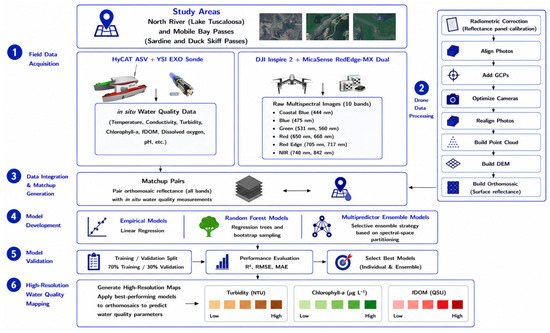
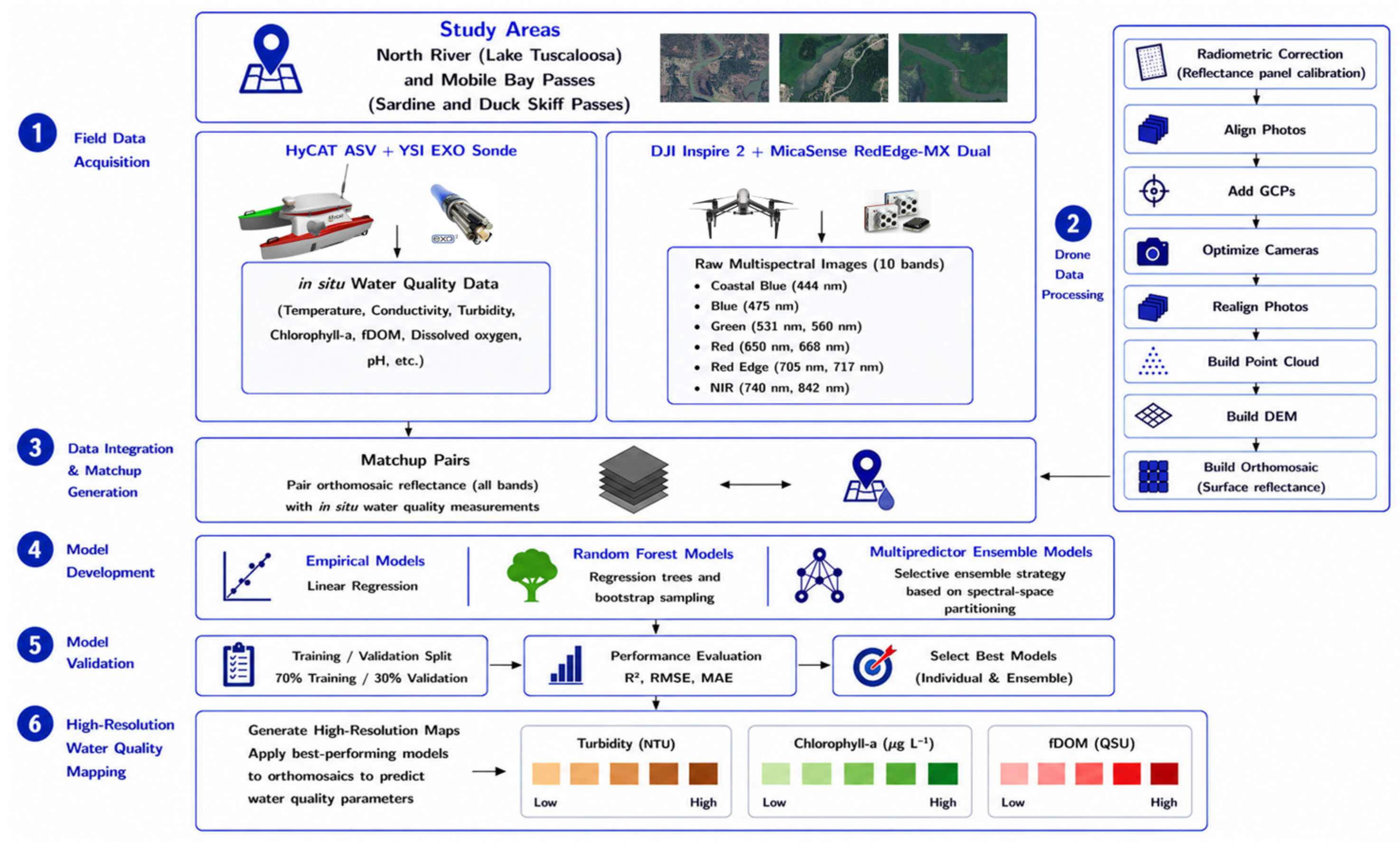
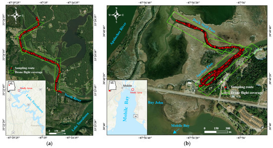
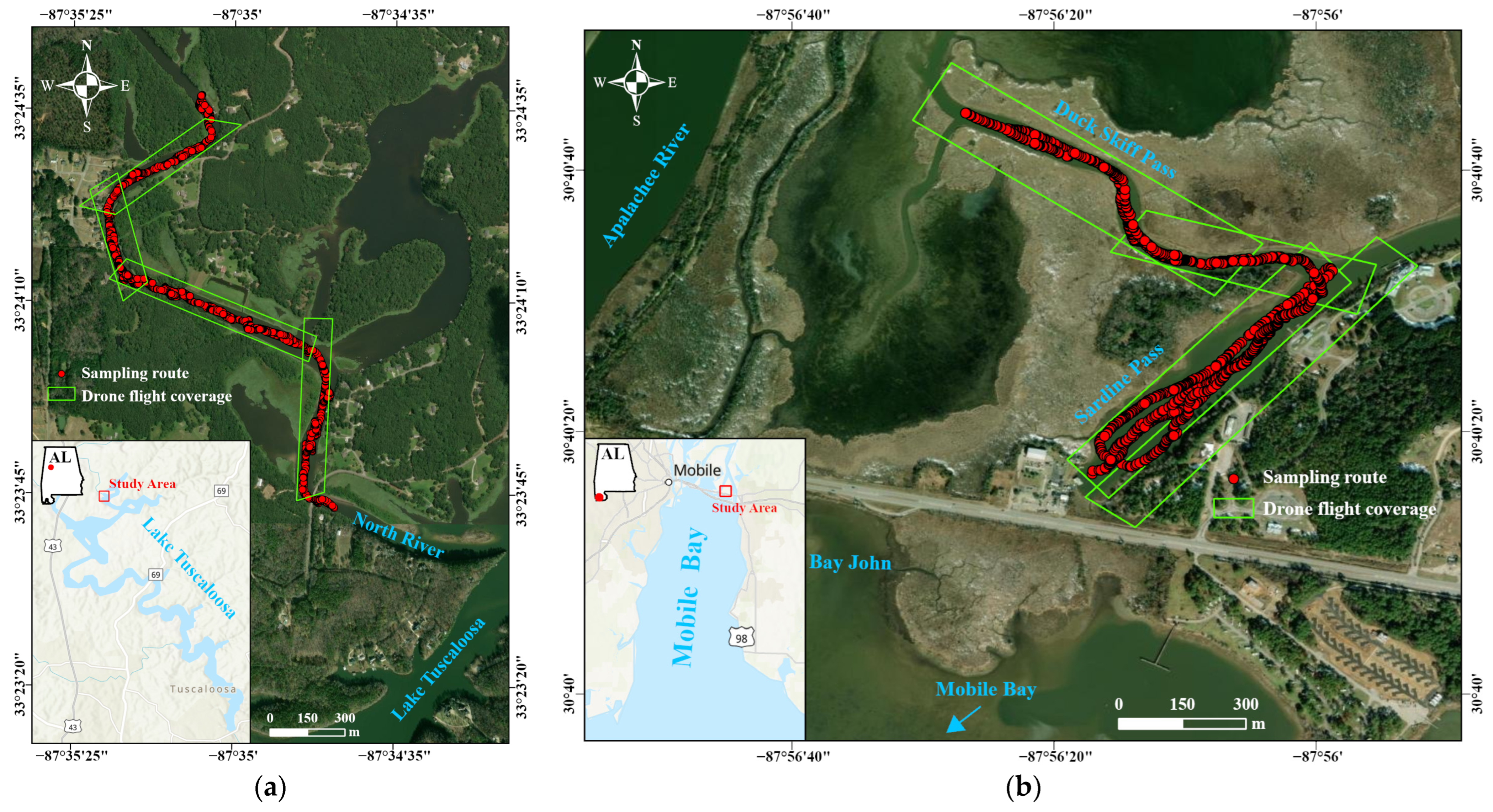
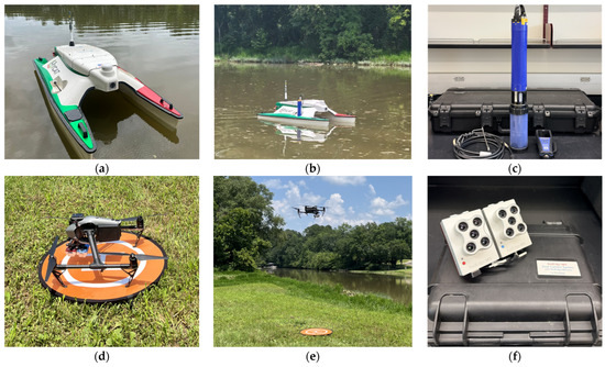
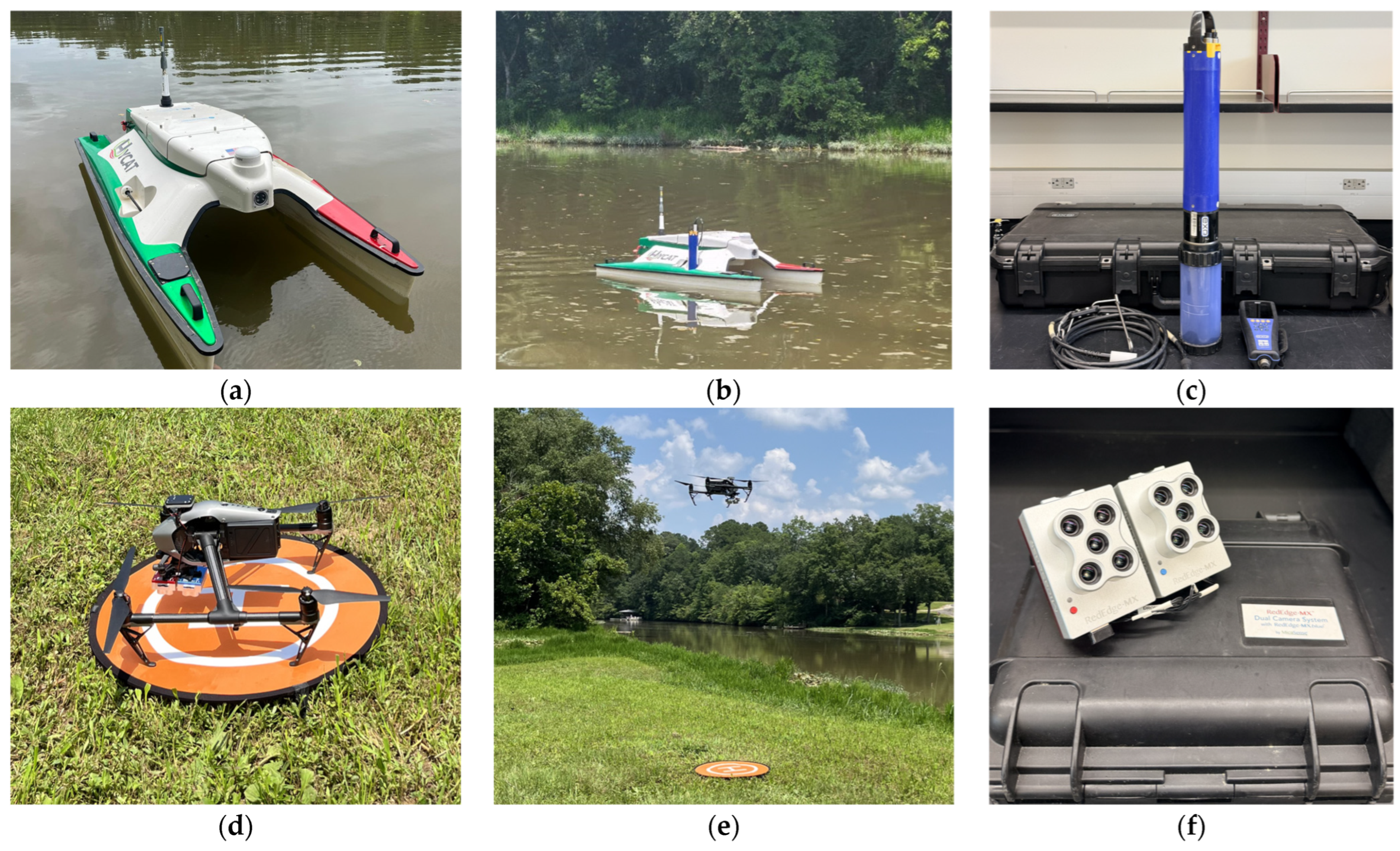
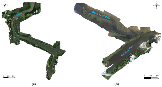
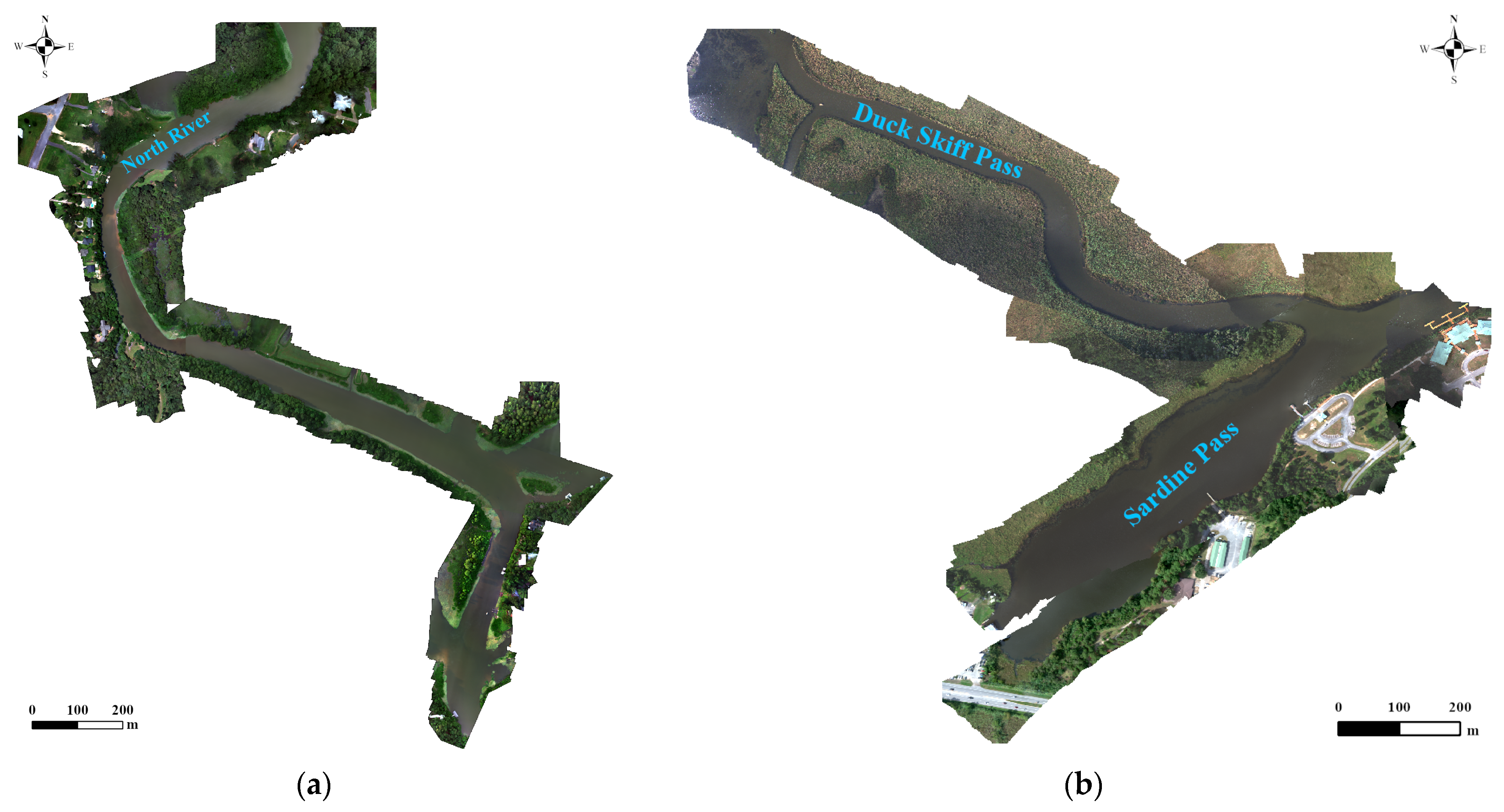
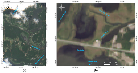
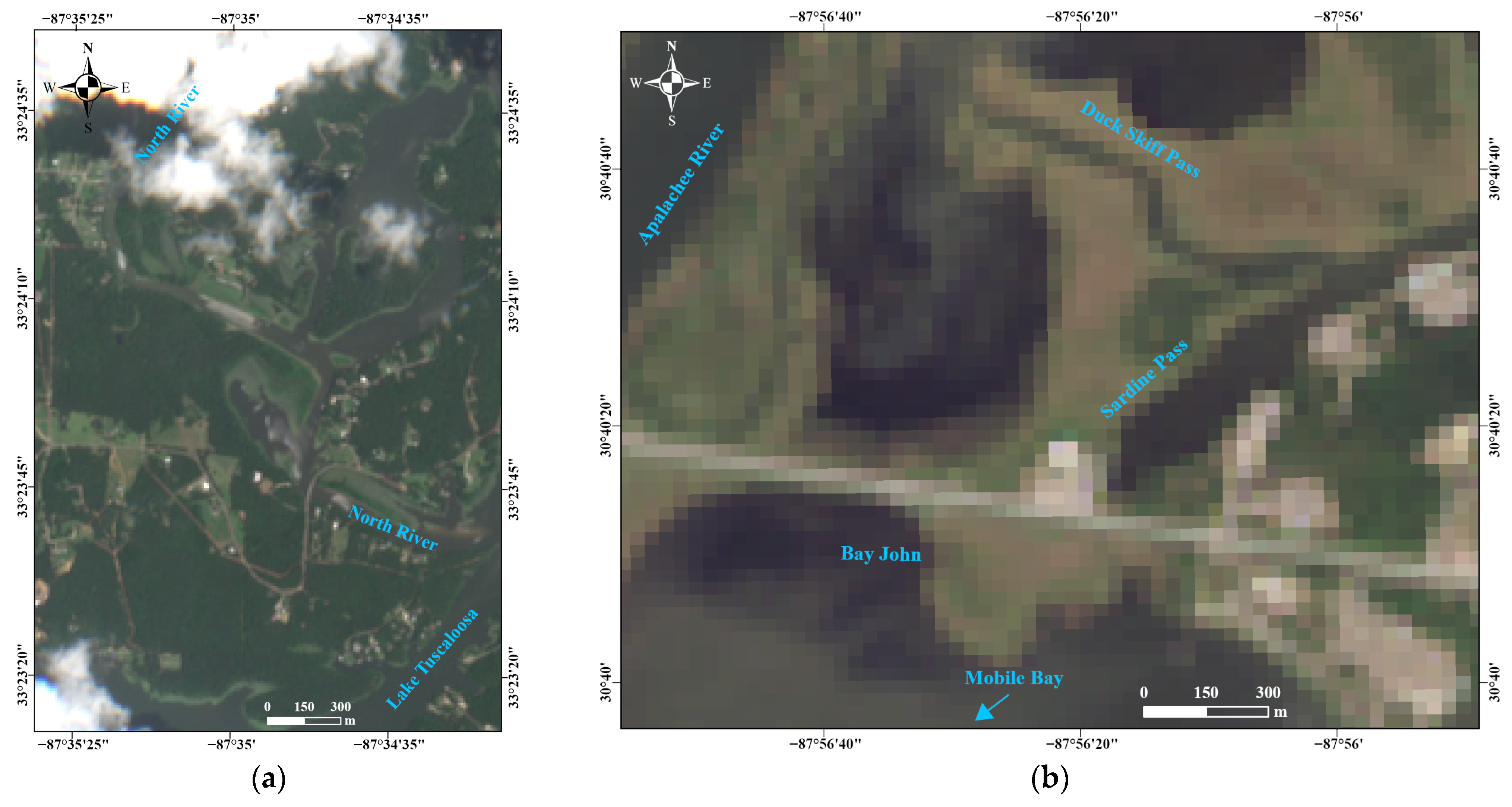
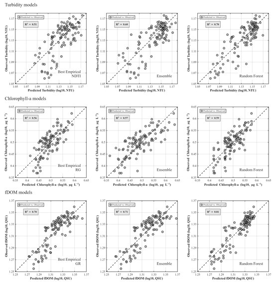
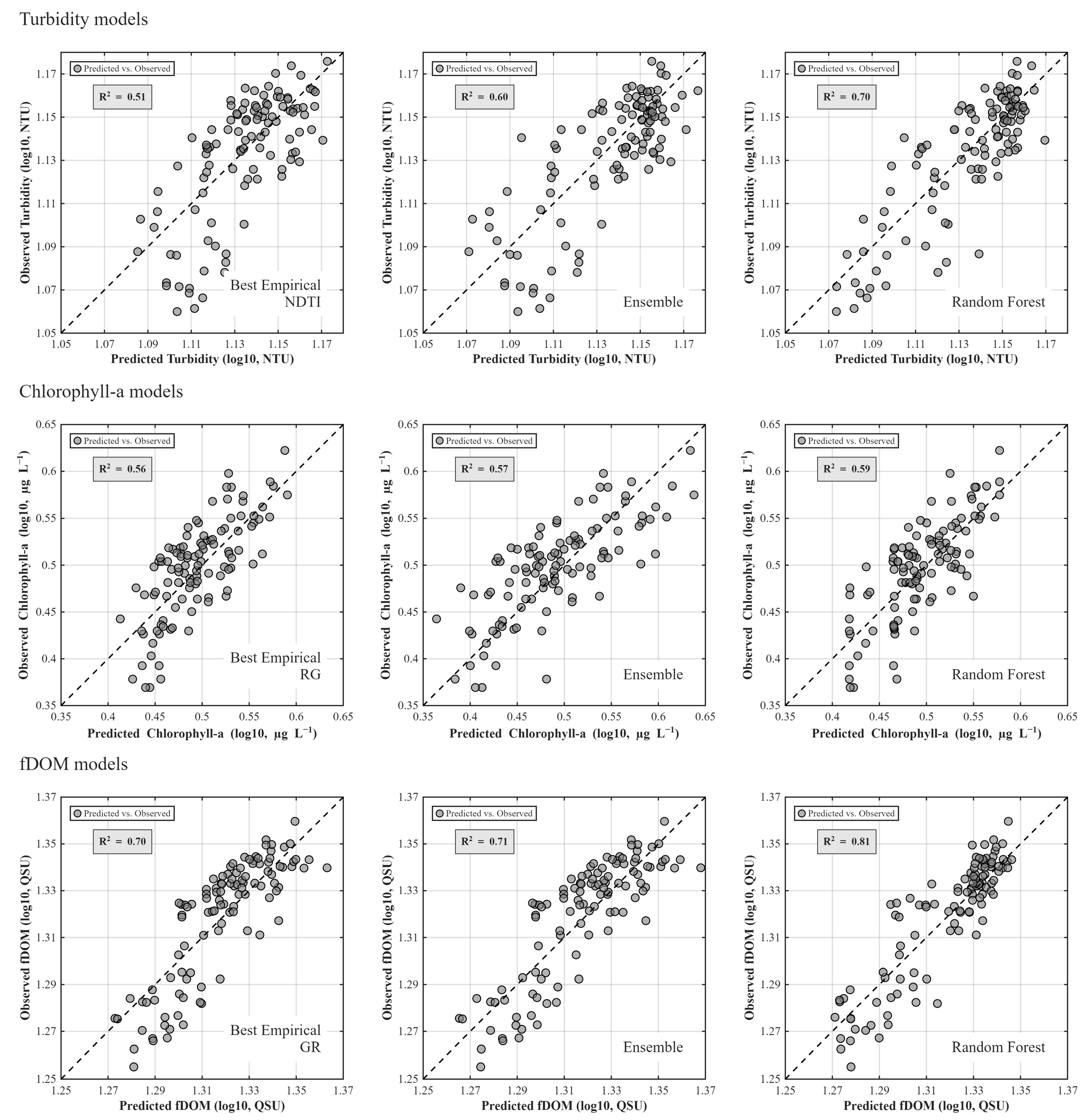
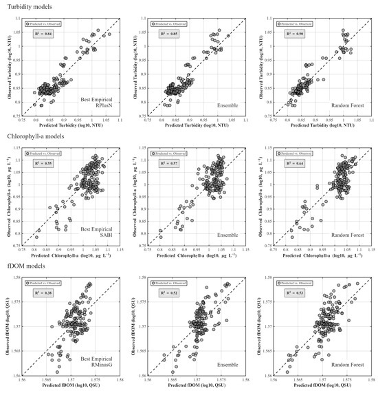
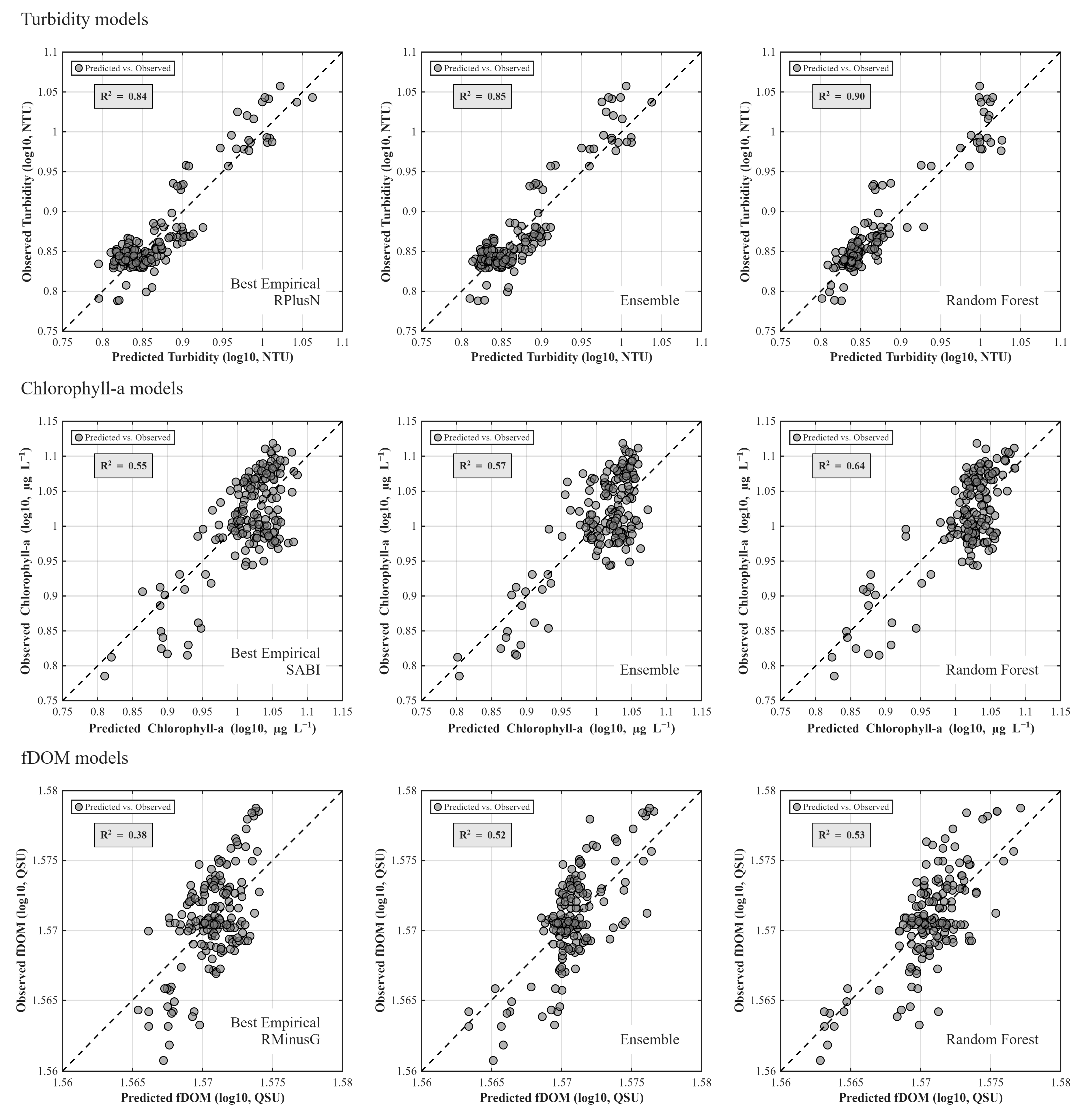
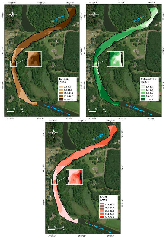
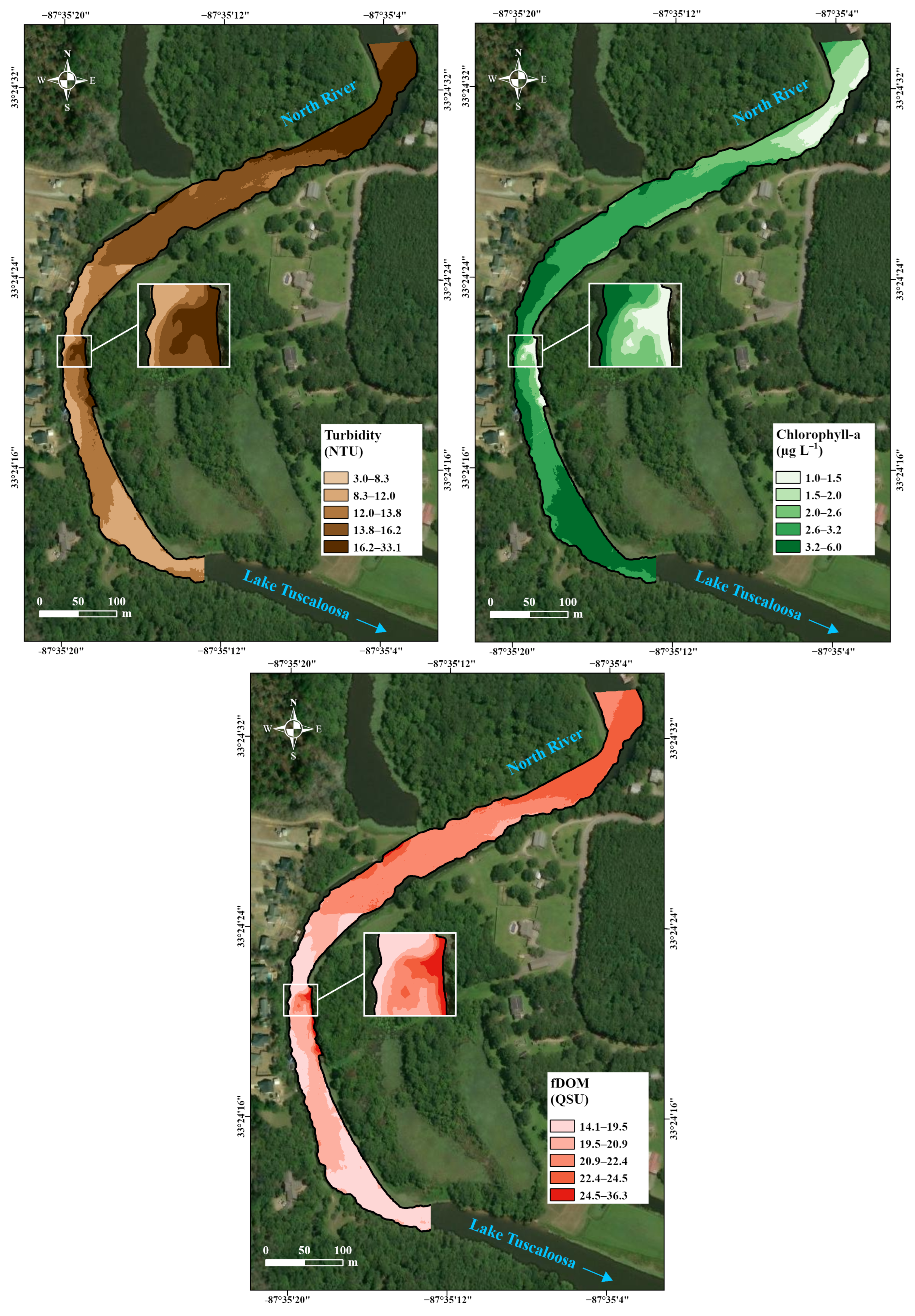
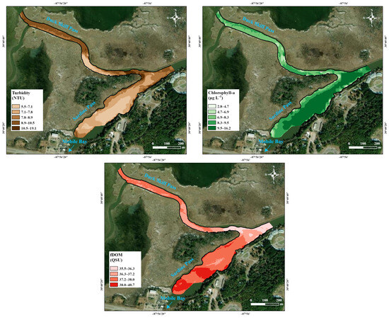
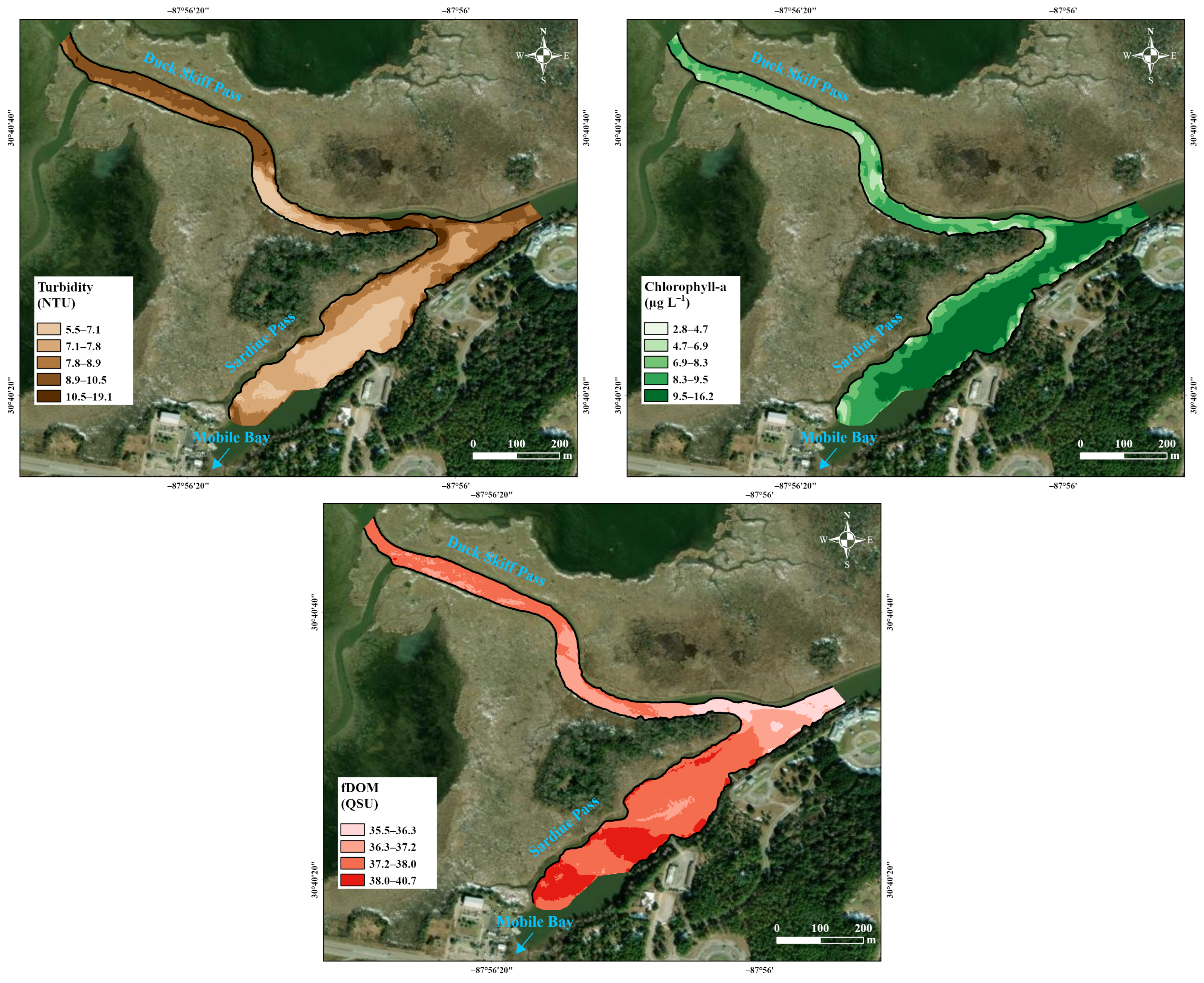
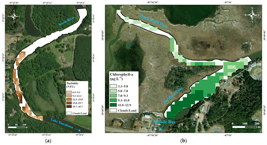
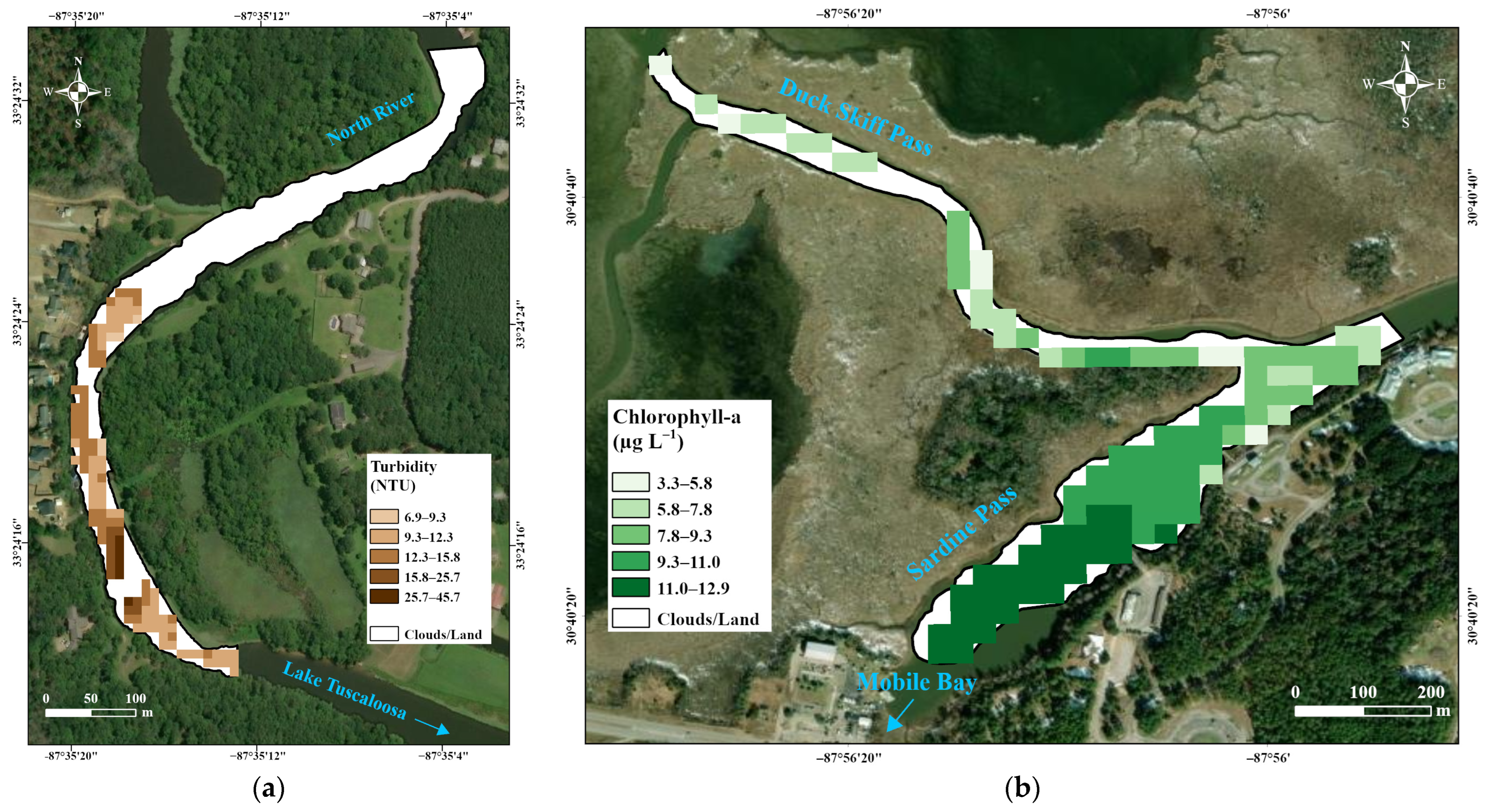

Disclaimer/Publisher’s Note: The statements, opinions and data contained in all publications are solely those of the individual author(s) and contributor(s) and not of MDPI and/or the editor(s). MDPI and/or the editor(s) disclaim responsibility for any injury to people or property resulting from any ideas, methods, instructions or products referred to in the content. |
© 2026 by the authors. Licensee MDPI, Basel, Switzerland. This article is an open access article distributed under the terms and conditions of the Creative Commons Attribution (CC BY) license.