SwinEADFormer: An Edge-Aware Dynamic Swin Transformer for Building Change Detection in High-Resolution Remote Sensing Images

Highlights

What are the main findings?

• SwinEADFormer conditions S3 cross-temporal interaction on image-pair-specific difference evidence and explicitly models the discrepancy between the two temporal directions.
• $\mathrm{\Phi }$ fusion combines directional interaction discrepancy with learned and direct S3 temporal differences. Five-seed ablations provide the strongest support for $\mathrm{\Phi }$ fusion and bidirectional interaction, while the router provides modest spatial modulation.

What are the implication of the main findings?

• Building change detection benefits from the coordination of interaction control, directional comparison, and direct difference preservation rather than relying on a single temporal interaction pathway.
• The proposed evidence chain addresses sparse changed regions while retaining structural information for region discrimination and boundary localization.

Abstract

Binary building change detection in high-resolution optical remote sensing images requires accurate temporal comparison and precise boundary localization. Existing methods often apply cross-temporal interaction uniformly to all spatial tokens at a selected feature level. When true changes are sparse, appearance differences at unchanged locations may still produce nonzero interaction responses. To address this issue, we propose SwinEADFormer, a difference-conditioned and discrepancy-aware cross-temporal interaction framework. A shared Swin-Tiny encoder extracts hierarchical bitemporal features. An image-pair-specific router generated from S3 difference cues and S4 semantic context modulates cross-temporal attention outputs before residual addition. The model explicitly computes the discrepancy between the two temporal interaction directions and fuses it with learned and direct S3 difference evidence. This design conditions interaction on estimated change evidence while preserving direct temporal differences. A multi-scale decoder produces the final change map. Experiments on LEVIR-CD, WHU-CD, and SYSU-CD show competitive region-level performance against representative baselines. On LEVIR-CD, SwinEADFormer achieves the highest mean B-recall and B-F1. Five-seed ablations show that $\mathrm{\Phi }$ fusion and bidirectional interaction provide the clearest improvements, while the router yields smaller mean gains.

1. Introduction

High-resolution remote sensing image change detection aims to identify land-cover or object-level changes from multi-temporal observations acquired over the same geographical area [1,2,3]. Among different change detection tasks, building change detection is particularly important for the monitoring of urban expansion, land resource management, disaster assessment, and inspection of illegal construction. With the increasing availability of very-high-resolution optical imagery, this task requires not only semantic discrimination of changed buildings but also accurate localization of object boundaries. Deep learning-based change detection methods usually adopt Siamese networks or encoder–decoder architectures to extract paired temporal features and compare them in a shared representation space [4,5,6,7]. These methods have achieved clear improvements over traditional hand-crafted difference operators. However, convolutional features are mainly driven by local receptive fields and may be insufficient for the modeling of long-range spatial–temporal dependencies in complex urban scenes. Transformer-based methods alleviate this limitation by introducing global or window-based attention mechanisms [8,9,10,11,12]. However, temporal feature exchange or cross-temporal attention is often applied to every spatial token at the selected feature level without change-dependent spatial modulation. Illumination, shadows, texture variations, or slight misregistration may then produce nonzero interaction responses at unchanged locations. These responses contain little structural change evidence but can still be propagated to the decoder. We refer to such responses as redundant background responses.

For binary building change detection, three issues remain important. First, temporal differences caused by illumination variation, shadows, seasonal changes, or slight misregistration should be suppressed when they do not correspond to real structural changes. Second, temporal interaction should consider both directions because buildings may appear, disappear or be partially occluded between two acquisitions. Third, building changes usually have clear structural boundaries, while predictions with high region-level accuracy may still suffer from eroded, expanded, or fragmented contours.

These properties motivate a task-driven interaction-evidence design. Cross-temporal interaction is conditioned on image-pair-specific difference evidence, while the discrepancy between the two temporal directions is combined with learned and direct temporal differences. S3 features support difference construction and bidirectional interaction, S4 features provide coarse semantic context for spatial modulation, and S1–S2 features support spatial recovery. This organization links interaction control, directional comparison, and direct evidence preservation in a single architecture.

Accordingly, this paper proposes SwinEADFormer, an edge-aware dynamic Swin Transformer framework for binary building change detection. SwinEADFormer uses a shared Swin-Tiny encoder to extract hierarchical bitemporal features and constructs an explicit stage-3 (S3) difference representation by combining original temporal features, absolute differences, and element-wise products. Based on this representation and high-level semantic context, an image-pair-specific edge–region–semantic router generates a soft spatial gate from edge, region, and semantic cues. The router modulates bidirectional edge-aware dynamic (EAD) interaction between the two temporal features. The $\mathrm{\Phi }$ fusion module further combines interaction-aware temporal discrepancy with direct difference evidence. A multi-scale decoder then produces the final change map.

The main contributions of this work are summarized as follows:

• We formulate a difference-conditioned cross-temporal interaction design for sparse building change detection. Image-pair-specific difference cues modulate S3 attention outputs before residual addition, while the original query feature remains in the residual path.
• We explicitly model the discrepancy between the $T_1\to T_2$ and $T_2\to T_1$ interaction outputs and fuse it with learned and direct S3 temporal differences. This design coordinates interaction-derived evidence with untransformed structural difference evidence.
• We evaluate the proposed design on LEVIR-CD, WHU-CD, and SYSU-CD under a controlled five-seed protocol. The ablations show that $\mathrm{\Phi }$ fusion and bidirectional interaction provide the strongest empirical support, while the router provides modest spatial modulation.

2. Related Work

2.1. Deep Learning-Based Change Detection

Deep learning has become the dominant paradigm for remote sensing change detection [13,14,15,16,17]. Early convolutional methods usually adopted Siamese or encoder-decoder architectures to extract bitemporal features and predict change maps from feature differences [4,5,18,19,20]. Siamese networks are widely used because they process two temporal images with shared weights, making the extracted features more comparable in the same representation space. Generic visual architectures also establish residual, densely connected, and multi-scale feature representations [21,22,23]. In remote sensing change detection, models combine semantically aware dense representations, dense skip connections, deeply supervised branches, metric learning, recurrent temporal modeling, or attention mechanisms to improve feature discrimination and localization [6,7,24,25,26,27,28,29].

Despite their effectiveness, convolutional change detection models mainly rely on local receptive fields. For high-resolution building change detection, local features are useful for capturing edges and textures, but they may be insufficient to model long-range spatial context and complex temporal dependencies. Simple feature subtraction or concatenation may also respond to irrelevant appearance variations, such as illumination changes, shadows, and slight misregistration [4,6,30]. These limitations motivate the use of stronger contextual modeling and more selective temporal interaction mechanisms.

2.2. Transformer-Based Change Detection

Transformer architectures have recently been introduced into remote sensing change detection to model long-range dependencies and global context [8,9,11,12,31]. Representative methods use token-based or hierarchical Transformer structures to capture spatial–temporal relationships between bitemporal images. Compared with convolutional models, Transformer-based methods are better suited for the modeling of non-local interactions and large-scale contextual dependencies, which are important for complex urban scenes. Related vision Transformer studies in detection and segmentation also show that attention-based representations can serve as broad visual backbones [32,33,34]. Window-based Transformers further reduce the computational burden of global self-attention while preserving hierarchical multi-scale representations [10,35].

Several Transformer-based change detection methods, including BIT, ChangeFormer, Changer, and CTDFormer, perform temporal feature exchange or cross-temporal relation modeling at the selected feature level [11,12,30,36]. In the building datasets used here, unchanged pixels dominate the images (

Table 1. Patch-level data split used in the experiments. The changed-pixel ratio is computed from the binary masks over all splits of each dataset.

Dataset	Patch Size	Train	Val	Test	Changed Pixels (%)
LEVIR-CD	$256\times 256$	7120	1024	2048	4.65
WHU-CD	$256\times 256$	1134	126	690	5.96
SYSU-CD	$256\times 256$	12,000	4000	4000	21.83

). Therefore, appearance variations at unchanged locations may generate nonzero interaction responses that contain limited change evidence but are still propagated to the decoder. A spatially adaptive mechanism can reweight these responses toward structurally meaningful and potentially changed regions.

Recent preprints have also adapted foundation or multimodal models to change detection, including SAM-based adaptation, language-guided change detection, and diffusion-feature-based joint registration and change detection [37,38,39]. These studies address foundation-model transfer, text-guided change detection, or explicit misregistration handling. The controlled experiments in this paper use visual-only binary change detection benchmarks. LEVIR-CD and WHU-CD are building-focused, while SYSU-CD provides a broader change setting.

2.3. Difference Interaction and Boundary-Aware Modeling

Difference feature modeling is a key component of remote sensing change detection [4,6,40,41,42]. Common strategies include feature concatenation, absolute differencing, element-wise multiplication, and attention-based fusion. These operations provide temporal contrast, but they may also respond to illumination changes, shadows, seasonal effects, or slight misregistration. For building change detection, boundary quality is also important because changed buildings often have regular shapes and sharp contours [43,44,45,46,47]. Existing boundary-aware methods usually use edge information as auxiliary supervision, boundary refinement, or feature enhancement. In contrast, SwinEADFormer uses the edge cue as one component of a router that modulates cross-temporal attention outputs.

2.4. Difference Relative to Existing Methods

BIT and ChangeFormer model bitemporal dependencies through token-based or hierarchical Transformer representations [11,12]. Changer further introduces feature exchange and alignment-based fusion for bitemporal interaction [30]. SwinEADFormer instead applies an image-pair-specific edge–region–semantic router to the outputs of S3 cross-temporal attention in both temporal directions. The discrepancy between the two directional outputs is then fused with direct S3 difference evidence through $\mathrm{\Phi }$ fusion.

Edge-CVT uses edge-informed modules to strengthen change representation and preserve building boundaries [46]. SwinEADFormer uses the edge response as one component of a soft interaction gate. The edge, region, and semantic cues jointly generate the router, which directly reweights the cross-temporal attention outputs.

SwinEADFormer follows a unified interaction-evidence chain. Image-pair-specific difference cues first condition the spatial amplitude of S3 cross-temporal attention outputs. The two temporal directions are then compared through the absolute discrepancy of their interaction outputs rather than being only added or concatenated. This discrepancy is finally fused with learned and direct S3 differences. The design therefore links difference construction, interaction control, directional comparison, and direct evidence preservation within one mechanism.

3. Materials and Methods

3.1. Overall Architecture

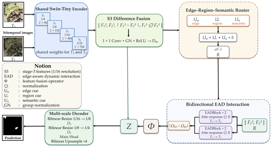
Given a pair of co-registered bitemporal images, $I_1$ and $I_2$, the goal of binary building change detection is to predict a change probability map ($\widehat{Y}$) indicating changed building regions. As shown in Figure 1, the proposed SwinEADFormer follows a shared Siamese encoder–decoder architecture. A shared Swin-Tiny encoder first extracts hierarchical features from the two temporal images [10]. Then, a stage-3 (S3) difference fusion module at $1/16$ input resolution constructs a mid-level difference representation. Based on this representation and high-level semantic context, an image-pair-specific edge–region–semantic router generates a soft spatial gate. The router is used to modulate bidirectional edge-aware dynamic (EAD) interaction between the two temporal features. Finally, the $\mathrm{\Phi }$ fusion module integrates interaction-aware discrepancy and direct difference evidence, and a multi-scale decoder produces the final change prediction.

Four connected choices define this interaction-evidence design. First, the router is generated from the current image pair using S3 edge and region cues, together with S4 semantic context. Second, the router gates the cross-temporal attention output before residual addition, preserving the original query feature in the identity path. Third, the two temporal directions are compared through the discrepancy of their interaction outputs. Fourth, this discrepancy is fused with learned and direct S3 difference evidence. These choices condition temporal interaction on estimated change evidence without making the final representation depend only on transformed attention features.

The shared encoder produces four-stage hierarchical features for each temporal image, as defined in Equation (1):

$$\{F_i^1,F_i^2,F_i^3,F_i^4\}=E\left(I_i\right),i\in \{1,2\},$$

(1)

Here, $F_i^1$, $F_i^2$, $F_i^3$, and $F_i^4$ denote the four encoder-stage features. For an input image of size $H_0\times W_0$, their dimensions are $F_i^1\in {\mathbb{R}}^{B\times 96\times H_0/4\times W_0/4}$, $F_i^2\in {\mathbb{R}}^{B\times 192\times H_0/8\times W_0/8}$, $F_i^3\in {\mathbb{R}}^{B\times 384\times H_0/16\times W_0/16}$, and $F_i^4\in {\mathbb{R}}^{B\times 768\times H_0/32\times W_0/32}$. The shared encoder weights ensure that the two temporal images are mapped into a comparable representation space.

All GroupNorm layers in the proposed modules use eight groups. A feature tensor with C channels is divided into groups of $C/8$ channels.

The overall design follows a coarse-to-fine strategy: S3 features support difference construction and router-guided interaction, high-level features provide semantic context for the router, and shallow features are used as decoder skips for spatial recovery. This design avoids applying cross-temporal attention at every encoder stage. The interaction is performed only at S3, where changed building structures remain spatially distinguishable and the features are more semantically reliable than shallow responses.

3.2. S3 Difference Fusion

Direct subtraction of two temporal features may be sensitive to illumination changes, shadows, and slight registration errors. To obtain a more discriminative mid-level difference representation, we construct an explicit fused difference feature at the S3 level by combining original temporal features, the absolute difference, and the element-wise product, as shown in Equation (2):

$$D_m={\varphi }_d\left(\left[F_1^3,F_2^3,|F_1^3-F_2^3|,F_1^3\odot F_2^3\right]\right),$$

(2)

Here, $[·]$ denotes channel-wise concatenation and ⊙ denotes element-wise multiplication. The ${\varphi }_d(·)$ operator uses a $1\times 1$ convolution to project the concatenated 1536-channel tensor to 384 channels, followed by GroupNorm with eight groups and ReLU activation. Here, S3 refers to $F_i^3$, the third encoder stage at $1/16$ input resolution. This feature level is selected because it provides a balance between semantic abstraction and spatial detail, which is important for distinguishing building changes while preserving object-level structures.

We also use the high-level semantic difference in Equation (3):

$$D_h=|F_1^4-F_2^4|,$$

(3)

which provides coarse semantic context for subsequent router generation.

3.3. Image-Pair-Specific Edge–Region–Semantic Router

At S3, cross-temporal attention produces interaction responses for all spatial tokens. Since unchanged regions dominate the image, appearance differences in these regions may introduce responses unrelated to true building changes. To suppress such responses, the image-pair-specific edge–region–semantic router generates a soft spatial gate for reweighting of the attention outputs.

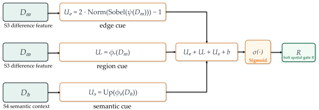
The router combines three cues with complementary spatial roles. The edge cue describes local structural transitions, but edge responses alone are insufficient because unchanged buildings, roads, and shadows may also produce strong local gradients. The region cue provides compact change evidence at S3, while the semantic cue supplies coarser contextual guidance from S4. Their combination estimates the spatial relevance of cross-temporal interaction responses rather than producing three independent change predictions. The edge cue is a Sobel response computed from a learned feature map, whereas the boundary target described in Section 3.5 is a binary supervision map derived from the ground-truth change mask. The three router cues are defined as follows:

$$\begin{array}{cc}\hfill U_e& =2·Norm\left(Sobel\left(\psi \left(D_m\right)\right)\right)-1,\hfill \\ \hfill U_r& ={\varphi }_r\left(D_m\right),\hfill \\ \hfill U_s& =Up\left({\varphi }_s\left(D_h\right)\right),\hfill \end{array}$$

(4)

The $\psi (·)$ projection applies group normalization with eight groups, followed by a bias-free $1\times 1$ convolution that maps $D_m$ to a single-channel feature (G). The Sobel operator uses the fixed kernels ($K_x=\left[\begin{array}{ccc}-1& 0& 1\\ -2& 0& 2\\ -1& 0& 1\end{array}\right]$ and $K_y=\left[\begin{array}{ccc}-1& -2& -1\\ 0& 0& 0\\ 1& 2& 1\end{array}\right]$), with a stride of 1 and padding of 1. The directional responses are $G_x=G\ast K_x$ and $G_y=G\ast K_y$, where ∗ denotes convolution. The edge magnitude is $M=\sqrt{G_x^2+G_y^2+ϵ}$, with $ϵ={10}^{-6}$. For each sample, it is normalized as $Norm\left(M\right)=clip\left(M/({max}_{h,w}M+ϵ),0,1\right)$ and rescaled from $[0,1]$ to $[-1,1]$ to obtain $U_e$.

The $Up(·)$ operator denotes bilinear interpolation and resizes the semantic logit map to the spatial resolution of $D_m$. The ${\varphi }_r(·)$ and ${\varphi }_s(·)$ projections share the same architecture but use independent parameters. Each projection consists of a $3\times 3$ convolution with a stride of 1 and padding of 1, group normalization with eight groups, ReLU activation, and a $1\times 1$ convolution that outputs a single-channel logit map.

The router map is then obtained by combining the three cues with a learnable bias, as given in Equation (5):

$$R=\sigma (U_e+U_r+U_s+b),$$

(5)

Here, b is a learnable scalar bias, and $\sigma (·)$ denotes the sigmoid function. The bias is initialized to $-1.0$ to provide a negative prior because changed pixels are usually sparse. The edge cue ($U_e$) is explicitly bounded in $[-1, 1]$. The region cue ($U_r$) and semantic cue ($U_s$) are learned logit maps. Their intermediate features are processed by group normalization, but their final logits and the learnable bias (b) are not explicitly clipped or bounded.

The router-logit scale is moderated by group normalization in the region and semantic branches, the initial bias ($b=-1.0$), the router edge loss, the sparsity loss, and gradients from the prediction losses. No explicit clipping is applied to $U_r$, $U_s$, or b, so large logit magnitudes may still saturate the sigmoid.

The R gate is broadcast along the channel dimension and multiplies the cross-temporal attention output before residual addition. This placement preserves the original query feature in the residual path and treats the router as a controller of the interaction increment rather than as a mask on the original representation. All spatial tokens remain in the attention computation; the gate changes only the spatial amplitude of the resulting interaction responses and does not reduce the attention FLOPs.

Figure 2 illustrates how edge, region, and semantic cues are combined in the router map (R) for subsequent cross-temporal attention.

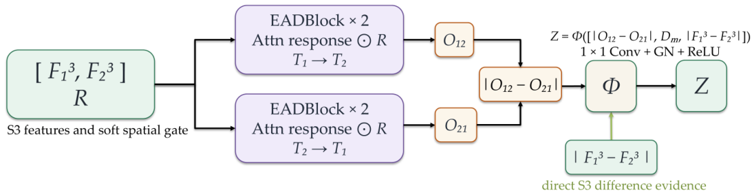
3.4. Bidirectional EAD Interaction and Φ Fusion

Given the paired S3 features ($F_1^3$ and $F_2^3$) and the router map (R), we perform router-guided, bidirectional edge-aware dynamic (EAD) interaction. Cross-temporal attention is directional because the query and reference features play different roles. We therefore compute both $T_1\to T_2$ and $T_2\to T_1$ interactions. The forward direction uses $F_1^3$ as the query feature and $F_2^3$ as the reference feature, while the reverse direction exchanges their roles. These two directions provide the basis for explicit modeling of direction-dependent interaction discrepancy, as formulated in Equations (6) and (7):

$$O_{12}={EAD}^{\left(2\right)}(F_1^3,F_2^3,R),$$

(6)

$$O_{21}={EAD}^{\left(2\right)}(F_2^3,F_1^3,R),$$

(7)

where ${EAD}^{\left(2\right)}(X,Y,R)$ denotes two consecutive EAD blocks that use the same reference feature (Y) and router map (R).

Each EAD block contains cross-temporal attention, router-based output gating, and a convolutional feed-forward network. Let $X,Y\in {\mathbb{R}}^{B\times C\times H\times W}$ denote the query and reference features, respectively, and let $R\in {\mathbb{R}}^{B\times 1\times H\times W}$ denote the router map. The router is broadcast along the channel dimension. The EAD block is defined as

$$\tilde{X}=Attn\left(GN\left(X\right),GN\left(Y\right)\right)\odot R,$$

(8)

$$X^{\prime }=X+\tilde{X},$$

(9)

$$EAD(X,Y,R)=X^{\prime }+0.5MLP\left(GN\left(X^{\prime }\right)\right).$$

(10)

The MLP takes the normalized residual feature ($GN\left(X^{\prime }\right)$) as input. It consists of a $1\times 1$ convolution that expands the channel dimension from C to $4C$, a GELU activation, and a second $1\times 1$ convolution that projects the feature back to C channels. The $0.5$ factor is fixed in all experiments. The router gates the attention output before the residual addition, while the original query feature (X) remains unchanged in the residual path.

The two directional outputs are not directly added or concatenated. Their absolute discrepancy is explicitly modeled as interaction-derived change evidence and is then integrated with learned and direct S3 difference evidence through the $\mathrm{\Phi }$ fusion module in Equation (11):

$$Z=\mathrm{\Phi }\left(\left[|O_{12}-O_{21}|,D_m,|F_1^3-F_2^3|\right]\right),$$

(11)

Here, $[·]$ denotes channel-wise concatenation. Each of the $|O_{12}-O_{21}|$, $D_m$, and $|F_1^3-F_2^3|$ inputs belongs to ${\mathbb{R}}^{B\times C\times H\times W}$, with $C=384$ in the Swin-Tiny implementation. Their concatenation is projected from $3C$ to C channels by a $1\times 1$ convolution, followed by group normalization with eight groups and ReLU activation, producing $Z\in {\mathbb{R}}^{B\times C\times H\times W}$. The three inputs provide bidirectional interaction discrepancy, learned S3 difference features, and direct temporal-difference evidence, respectively. Thus, $\mathrm{\Phi }$ fusion is a lightweight convolutional fusion operator rather than an additional attention module.

Figure 3 shows how the router-gated bidirectional branches are fused with direct stage-3 (S3) difference evidence to obtain Z.

The absolute discrepancy ($|O_{12}-O_{21}|$) captures differences between the two directional interaction outputs. It is fused with $D_m$ and $|F_1^3-F_2^3|$ to combine interaction-derived, learned, and direct temporal-difference evidence.

3.5. Decoder and Training Objective

To recover spatial details, the multi-scale decoder progressively fuses Z with lower-level absolute-difference skip features. Let ${\mathcal{U}}_{h,w}\left(X\right)$ denote bilinear interpolation of X to a spatial size of $h\times w$. The first decoder stage is defined as

$$D_3={\rho }_3\left(\left[{\mathcal{U}}_{H_0/8,W_0/8}\left(Z\right),|F_1^2-F_2^2|\right]\right),$$

(12)

The second decoder stage is defined as

$$D_2={\rho }_2\left(\left[{\mathcal{U}}_{H_0/4,W_0/4}\left(D_3\right),|F_1^1-F_2^1|\right]\right),$$

(13)

The decoder contains two refinement stages. First, Z is resized from $H_0/16\times W_0/16$ to $H_0/8\times W_0/8$ and concatenated with the 192-channel stage-2 absolute-difference feature. The resulting 576-channel tensor is processed by ${\rho }_3(·)$ through two $3\times 3$ convolutions with channel dimensions of $576\to 192\to 192$. Next, $D_3$ is resized to $H_0/4\times W_0/4$ and concatenated with the 96-channel stage-1 difference feature. The resulting 288-channel tensor is processed by ${\rho }_2(·)$ with channel dimensions of $288\to 96\to 96$. Each decoder convolution uses a stride of 1, padding of 1, GroupNorm with eight groups, and ReLU activation.

A $1\times 1$ convolution projects the 96-channel $D_2$ feature to one logit channel. The logit map is resized from $H_0/4\times W_0/4$ to $H_0\times W_0$ by bilinear interpolation:

$$P=\mathrm{Head}\left(D_2\right),\tilde{P}={Up}_4\left(P\right),\widehat{Y}=\sigma \left(\tilde{P}\right).$$

(14)

The training objective combines the final prediction loss, an auxiliary prediction loss, a router edge loss, and a router sparsity loss. A $1\times 1$ auxiliary head projects the 384-channel feature (Z) to the single-channel logit ($P_{aux}$). The auxiliary logit and router map are resized to the input resolution by bilinear interpolation, producing ${\tilde{P}}_{aux}$ and $\tilde{R}$. The total loss is

$$\mathcal{L}={\mathcal{L}}_{main}+{\lambda }_{aux}{\mathcal{L}}_{aux}+{\lambda }_{edge}{\mathcal{L}}_{edge}+{\lambda }_s{\mathcal{L}}_{sparse}.$$

(15)

The main and auxiliary branches use the same prediction loss. For a prediction logit map (Q), we first compute the bounded probability map:

$$S=clip\left(\sigma \left(Q\right),{10}^{-6},1-{10}^{-6}\right).$$

(16)

The prediction loss is defined as

$${\mathcal{L}}_{pred}(Q,Y)={\mathcal{L}}_{focal}(Q,Y)+{\mathcal{L}}_{dice}(S,Y)+0.4{\mathcal{L}}_{bc}(S,Y).$$

(17)

The binary focal loss [48] uses ${\alpha }_f=0.5$ and $\gamma =2.0$. Specifically,

$$\begin{array}{cc}\hfill p_t& =S\odot Y+(1-S)\odot (1-Y),\hfill \\ \hfill {\alpha }_t& ={\alpha }_{f}Y+(1-{\alpha }_f)(1-Y),\hfill \\ \hfill {\mathcal{L}}_{focal}& =mean\left[{\alpha }_t{(1-p_t)}^{\gamma }{\mathit{\ell }}_{\mathrm{BCE}}(Q,Y)\right],\hfill \end{array}$$

(18)

Here, ${\mathit{\ell }}_{\mathrm{BCE}}(Q,Y)$ denotes the unreduced pixel-wise binary cross-entropy-with-logits term.

The Dice loss [49] is computed independently for each image, then averaged over the batch:

$${\mathcal{L}}_{dice}=1-{\displaystyle \frac{1}{B}}{\displaystyle \sum _{i=1}^B}{\displaystyle \frac{2{\sum }_{h,w}{S}_i{Y}_i+{10}^{-5}}{{\sum }_{h,w}{S}_i+{\sum }_{h,w}{Y}_i+{10}^{-5}}}.$$

(19)

For the boundary-consistency term, we use the fixed Laplacian kernel:

$$K=\left[\begin{array}{ccc}0& 1& 0\\ 1& -4& 1\\ 0& 1& 0\end{array}\right].$$

(20)

The soft Laplacian boundary response for an input map (X) is defined as $\mathcal{B}\left(X\right)=|X\ast K|$, where ∗ denotes convolution with a padding of 1.

$${\mathcal{L}}_{bc}(S,Y)=mean\left(\left|\mathcal{B}\left(S\right)-\mathcal{B}\left(Y\right)\right|\right).$$

(21)

The prediction boundary is computed from the sigmoid probability map (S), while the target boundary is computed from the binary ground-truth mask (Y). Neither boundary response is binarized in ${\mathcal{L}}_{bc}$. Their discrepancy is measured using the mean absolute error. Therefore, the main and auxiliary losses are

$${\mathcal{L}}_{main}={\mathcal{L}}_{pred}(\tilde{P},Y),{\mathcal{L}}_{aux}={\mathcal{L}}_{pred}({\tilde{P}}_{aux},Y).$$

(22)

The router edge loss constrains the resized router map using a Laplacian-derived binary target:

$${\mathcal{L}}_{edge}=\mathrm{BCE}\left(\tilde{R},\mathrm{EdgeGT}\left(Y\right)\right),$$

(23)

$$\mathrm{EdgeGT}\left(Y\right)=\mathbb{I}\left(|Y\ast K|>0\right),$$

(24)

Here, K is the fixed $3\times 3$ Laplacian kernel in Equation (20), and the convolution uses a padding of 1. The indicator function ($\mathbb{I}(·)$) converts the absolute Laplacian response into a binary edge target. The resized router map ($\tilde{R}$) is clipped to $[{10}^{-6}, 1-{10}^{-6}]$ before binary cross-entropy is computed.

The router sparsity loss is defined as

$${\mathcal{L}}_{sparse}={\displaystyle \frac{1}{BHW}}{\displaystyle \sum _{b=1}^B}{\displaystyle \sum _{h=1}^H}{\displaystyle \sum _{w=1}^W}{R}_{b,1,h,w},$$

(25)

The average is computed over all samples and spatial locations of the single-channel router map. The original router map (R) is used for sparsity regularization, while the resized map ($\tilde{R}$) is used for router-edge supervision.

The auxiliary, router-edge, and sparsity loss weights are fixed to ${\lambda }_{aux}=0.4$, ${\lambda }_{edge}=0.2$, and ${\lambda }_s={10}^{-4}$, respectively. The coefficient of the boundary-consistency term in ${\mathcal{L}}_{pred}$ is fixed to 0.4. These coefficients are fixed across all experiments, and the validation set is used only for checkpoint selection according to the F1 score.

4. Results

4.1. Experimental Setup

We evaluate SwinEADFormer on three public optical binary change detection datasets: LEVIR-CD [50], WHU-CD [51], and SYSU-CD [29]. All images used in our experiments contain three visible bands—namely, red, green, and blue. No near-infrared, multispectral, or SAR channels are used. LEVIR-CD and WHU-CD are building-focused benchmarks, whereas SYSU-CD contains both building and non-building changes. Table 1 reports the patch-level splits used in our experiments.

LEVIR-CD contains Google Earth images collected from urban and suburban regions in Texas, USA. The images have a spatial resolution of 0.5 m per pixel, and the acquisition dates span from 2002 to 2018. The labeled changes mainly correspond to building construction and removal, while roads, vegetation, and other urban surfaces form complex backgrounds [50]. WHU-CD contains aerial images covering Christchurch, New Zealand, acquired in 2012 and 2016 with a spatial resolution of 0.2 m per pixel. It mainly captures building additions and removals during post-earthquake urban reconstruction. The scenes include residential and industrial buildings with different sizes and structural patterns, together with roads, vegetation, parking areas, and shadows [51]. SYSU-CD contains aerial images from Hong Kong, China, with a spatial resolution of 0.5 m per pixel, and its image pairs span from 2007 to 2014. Compared with LEVIR-CD and WHU-CD, SYSU-CD contains a wider range of change types, including urban construction, suburban expansion, vegetation change, road expansion, and coastal construction [29]. We therefore use SYSU-CD as a broader binary change detection benchmark rather than a purely building-specific dataset.

The changed-pixel ratios show clear class imbalance. Changed pixels account for only 4.65% and 5.96% of all pixels in LEVIR-CD and WHU-CD, respectively. SYSU-CD has a higher changed-pixel ratio of 21.83%, but unchanged pixels still dominate. We therefore report precision, recall, F1 score, and IoU, together with OA.

SwinEADFormer is implemented in PyTorch 2.5.1 with CUDA 12.1 using an ImageNet-pretrained Swin-Tiny encoder provided by timm 1.0.27. All bilinear interpolation operations are implemented in PyTorch with align_corners=False. All competing methods are retrained from the official implementations released by the corresponding authors. Their original architectures, method-specific modules, and training objectives are retained.

Within each dataset, all methods use the same data split, input resolution, paired data augmentation, optimizer, learning-rate schedule, training epochs, random seeds, checkpoint-selection rule, prediction threshold, and metric implementation. LEVIR-CD and WHU-CD are trained for 100 epochs with a batch size of 8. SYSU-CD is trained for 30 epochs with a batch size of 32, except for CDMamba, whose batch size is reduced to 8 because of GPU memory limits. AdamW [52] is used with an initial learning rate of $3\times {10}^{-5}$, a weight decay of ${10}^{-2}$, five warm-up epochs, and cosine decay. Method-specific settings outside this common protocol follow the corresponding official configurations.

All main comparisons and component ablations are repeated using the same five random seeds. For each run, the checkpoint with the highest validation F1 score is evaluated once on the test set. All five test results are included in the reported mean and standard deviation, and no run is selected according to test performance. Methods are ranked according to their mean values.

We report precision, recall, F1 score, IoU, and OA as region-level metrics. We also report boundary precision, boundary recall, boundary F1 score, and boundary IoU [44] as boundary-level metrics. For all methods, we extract boundary bands by symmetric morphology with a width of three pixels. We use a two-pixel matching tolerance for boundary F1, while boundary IoU is computed as the direct overlap of the extracted boundary bands.

4.2. Comparison with Representative Methods

We first compare SwinEADFormer with representative change detection methods on LEVIR-CD. The CNN-based baselines include FC-EF and FC-Siam variants [4], SNUNet-CD [7], and FCCDN [28]. The Transformer-based baselines include BIT [11] and ChangeFormer [12]. We also include recent interaction, boundary-aware, and sequence models, including Changer [30], ChangeMamba [53], Edge-CVT [46], and CDMamba [54].

Table 2. Region-level comparison on LEVIR-CD. Results are reported as mean ± standard deviation over five random seeds. The best mean value is shown in bold.

Method	Precision	Recall	F1	IoU	OA
CNN-based
FC-Siam-diff	$90.09\pm 0.05$	$83.50\pm 0.22$	$86.67\pm 0.11$	$76.48\pm 0.17$	$98.67\pm 0.01$
FC-EF	$90.12\pm 0.06$	$86.65\pm 0.12$	$88.35\pm 0.07$	$79.14\pm 0.12$	$98.82\pm 0.01$
FC-Siam-conc	$90.65\pm 0.16$	$87.36\pm 0.18$	$88.97\pm 0.12$	$80.14\pm 0.20$	$98.88\pm 0.01$
Nested/dense CNN
SNUNet-CD	$90.76\pm 0.09$	$88.09\pm 0.11$	$89.40\pm 0.07$	$80.84\pm 0.11$	$98.92\pm 0.01$
FCCDN	$90.62\pm 0.12$	$88.56\pm 0.08$	$89.58\pm 0.11$	$81.12\pm 0.18$	$98.94\pm 0.01$
Transformer-based
ChangeFormer	$90.30\pm 0.04$	$87.82\pm 0.14$	$89.04\pm 0.09$	$80.25\pm 0.14$	$98.88\pm 0.01$
BIT	$\mathbf{91.49}\mathbf{\pm }\mathbf{0.09}$	$87.17\pm 0.11$	$89.28\pm 0.10$	$80.64\pm 0.16$	$98.92\pm 0.01$
Recent interaction/edge-aware/state-space models
Changer	$90.07\pm 0.11$	$85.49\pm 0.09$	$87.72\pm 0.08$	$78.13\pm 0.13$	$98.76\pm 0.01$
ChangeMamba	$89.67\pm 0.09$	$86.80\pm 0.13$	$88.21\pm 0.06$	$78.91\pm 0.10$	$98.80\pm 0.01$
Edge-CVT	$90.96\pm 0.07$	$89.10\pm 0.14$	$90.02\pm 0.08$	$81.86\pm 0.13$	$98.98\pm 0.01$
CDMamba	$90.39\pm 0.11$	$88.40\pm 0.12$	$89.38\pm 0.10$	$80.80\pm 0.16$	$98.92\pm 0.01$
Proposed
SwinEADFormer	$91.14\pm 0.08$	$\mathbf{89.52}\mathbf{\pm }\mathbf{0.13}$	$\mathbf{90.32}\mathbf{\pm }\mathbf{0.07}$	$\mathbf{82.35}\mathbf{\pm }\mathbf{0.12}$	$\mathbf{99.01}\mathbf{\pm }\mathbf{0.01}$

and

Table 3. Boundary-level comparison on LEVIR-CD. Results are reported as mean ± standard deviation over five random seeds. The best mean value is shown in bold.

Method	B-Precision	B-Recall	B-F1	B-IoU
CNN-based
FC-Siam-diff	$91.46\pm 0.24$	$88.94\pm 0.18$	$90.18\pm 0.10$	$63.93\pm 0.19$
FC-EF	$92.62\pm 0.27$	$91.12\pm 0.15$	$91.86\pm 0.07$	$66.82\pm 0.21$
FC-Siam-conc	$92.35\pm 0.11$	$92.39\pm 0.12$	$92.37\pm 0.08$	$68.28\pm 0.19$
Nested/dense CNN
SNUNet-CD	$93.41\pm 0.21$	$92.56\pm 0.12$	$92.98\pm 0.06$	$69.44\pm 0.11$
FCCDN	$93.57\pm 0.08$	$93.01\pm 0.21$	$93.29\pm 0.13$	$69.31\pm 0.18$
Transformer-based
ChangeFormer	$93.46\pm 0.10$	$92.02\pm 0.15$	$92.73\pm 0.10$	$67.92\pm 0.15$
BIT	$\mathbf{96.01}\mathbf{\pm }\mathbf{0.12}$	$90.27\pm 0.22$	$93.05\pm 0.07$	$67.39\pm 0.17$
Recent interaction/edge-aware/state-space models
Changer	$92.53\pm 0.13$	$90.41\pm 0.16$	$91.46\pm 0.08$	$66.90\pm 0.15$
ChangeMamba	$90.26\pm 0.20$	$91.48\pm 0.18$	$90.87\pm 0.11$	$65.71\pm 0.14$
Edge-CVT	$93.93\pm 0.22$	$92.31\pm 0.16$	$93.11\pm 0.08$	$69.79\pm 0.21$
CDMamba	$94.09\pm 0.10$	$92.98\pm 0.17$	$93.53\pm 0.14$	$\mathbf{70.58}\mathbf{\pm }\mathbf{0.18}$
Proposed
SwinEADFormer	$95.54\pm 0.09$	$\mathbf{93.08}\mathbf{\pm }\mathbf{0.13}$	$\mathbf{94.29}\mathbf{\pm }\mathbf{0.10}$	$69.82\pm 0.15$

report the region-level and boundary-level metrics, respectively. The former evaluates overall changed-building prediction, while the latter reflects contour completeness and localization.

Table 2 reports the region-level results on LEVIR-CD. SwinEADFormer achieves the highest mean recall, F1 score, IoU, and OA among the compared methods. Compared with Edge-CVT, the strongest competing method in terms of mean F1 score and IoU, SwinEADFormer improves the F1 score from 90.02% to 90.32% and IoU from 81.86% to 82.35%. These correspond to gains of 0.30 and 0.49 percentage points, respectively. BIT achieves the highest precision, indicating a more conservative prediction tendency. Overall, SwinEADFormer provides a better balance between change-region completeness and false-alarm control.

Region-level and boundary-level metrics evaluate different aspects of the prediction. The F1 score and IoU measure the overlap of changed-building regions, but they may not fully reflect contour fragmentation or local boundary displacement. B-precision and B-recall evaluate boundary detection within the predefined matching tolerance, while B-IoU uses the direct overlap of boundary bands and therefore imposes a stricter localization requirement. A method may consequently recover more complete contours without achieving the highest B-IoU. We therefore analyze the boundary-level results separately.

Table 3 reports the boundary-level results on LEVIR-CD. SwinEADFormer achieves the highest mean B-recall and B-F1, while BIT obtains the highest B-precision and CDMamba achieves the highest B-IoU. SwinEADFormer obtains the second-highest B-IoU, although its advantage over Edge-CVT on this metric is marginal.

The different rankings across the boundary metrics reflect distinct prediction behaviors. BIT achieves the highest B-precision but a lower B-recall, indicating that its predicted boundaries are relatively conservative. CDMamba obtains the highest B-IoU, which suggests stronger strict overlap between the predicted and reference boundary bands. SwinEADFormer achieves the highest B-recall and B-F1. This result indicates that it recovers a larger proportion of the reference boundaries while maintaining a balanced precision–recall trade-off. The small difference between SwinEADFormer and Edge-CVT in B-IoU also shows that the gain is more evident under tolerance-based boundary matching than under strict boundary-band overlap. Therefore, the boundary results support improved contour completeness, but they do not indicate uniform superiority under every boundary criterion.

4.3. Ablation Study

To assess the contribution of each component, we conduct five-seed ablation experiments on LEVIR-CD.

Table 4. Multi-seed component ablation on LEVIR-CD using $256\times 256$ input patches. Results are reported as mean ± standard deviation over five random seeds. The best mean value is shown in bold.

Variant	F1	IoU	B-F1	B-IoU
Full	$\mathbf{90.32}\mathbf{\pm }\mathbf{0.07}$	$\mathbf{82.35}\mathbf{\pm }\mathbf{0.12}$	$\mathbf{94.29}\mathbf{\pm }\mathbf{0.10}$	$\mathbf{69.82}\mathbf{\pm }\mathbf{0.15}$
w/o $\mathrm{\Phi }$ fusion	$89.73\pm 0.11$	$81.37\pm 0.10$	$93.75\pm 0.13$	$68.32\pm 0.12$
w/o router	$90.12\pm 0.08$	$82.02\pm 0.14$	$94.17\pm 0.10$	$69.38\pm 0.10$
Unidirectional interaction	$89.88\pm 0.09$	$81.62\pm 0.11$	$93.68\pm 0.12$	$68.44\pm 0.15$
Semantic cue only (s)	$90.27\pm 0.05$	$82.27\pm 0.13$	$94.15\pm 0.12$	$69.52\pm 0.16$
w/o edge cue ($r+s$)	$90.12\pm 0.09$	$82.02\pm 0.13$	$94.16\pm 0.05$	$69.41\pm 0.11$

reports the mean and standard deviation over the five runs. The tested variants remove or simplify $\mathrm{\Phi }$ fusion, the dynamic router, bidirectional interaction, and the router’s cue composition.

In the w/o $\mathrm{\Phi }$ fusion variant, the model uses only the bidirectional interaction discrepancy ($|O_{12}-O_{21}|$) and excludes $D_m$ and $|F_1^3-F_2^3|$ from the final fusion, while all other settings remain unchanged.

Removing $\mathrm{\Phi }$ fusion decreases the F1 score, IoU, B-F1, and B-IoU by 0.59, 0.98, 0.54, and 1.50 percentage points, respectively. These reductions show that combining interaction-aware discrepancy with direct difference evidence is important for both region prediction and strict boundary overlap.

Replacing bidirectional interaction with unidirectional interaction decreases the F1 score, IoU, B-F1, and B-IoU by 0.44, 0.73, 0.61, and 1.38 percentage points, respectively. These reductions show that the two temporal directions provide complementary evidence for both region prediction and boundary recovery. The effect is more pronounced on the boundary metrics, which suggests that bidirectional interaction is particularly helpful for recovering boundary continuity and reducing local fragmentation.

Removing the router decreases the mean F1 score, IoU, B-F1, and B-IoU by 0.20, 0.33, 0.12, and 0.44 percentage points, respectively. The full configuration also achieves higher mean values than the semantic-only variant on all four metrics, with differences of 0.05, 0.08, 0.14, and 0.30 points. These margins remain small and are largest in B-IoU. The results indicate that the complete cue configuration provides modest mean improvements, mainly in boundary overlap.

Taken together, these ablations support the proposed interaction-evidence chain. The larger degradations caused by removing $\mathrm{\Phi }$ fusion and replacing bidirectional interaction with a unidirectional variant indicate that explicit directional comparison and the fusion of interaction-derived and direct difference evidence are the most strongly supported design choices. The smaller but consistent router-related changes show that difference-conditioned routing provides secondary spatial modulation, mainly for strict boundary overlap.

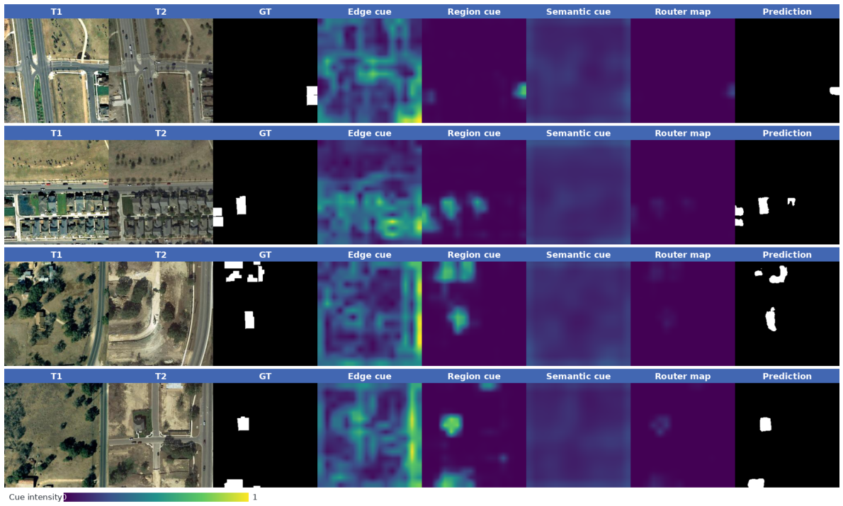
Figure 4 visualizes the three router cues and the final router map. The edge cue highlights local structural transitions, the region cue responds to candidate changed areas, and the semantic cue provides smoother contextual guidance. The final router map assigns stronger responses to structurally relevant locations. This pattern is consistent with Table 4, where the complete cue configuration is shown to achieve modest gains over the reduced variants.

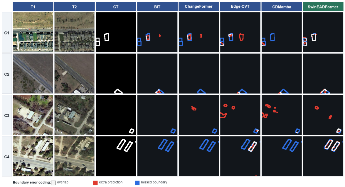
Figure 5 and Figure 6 show region predictions and boundary errors for the same test cases. They complement the quantitative results in Table 2 and Table 3.

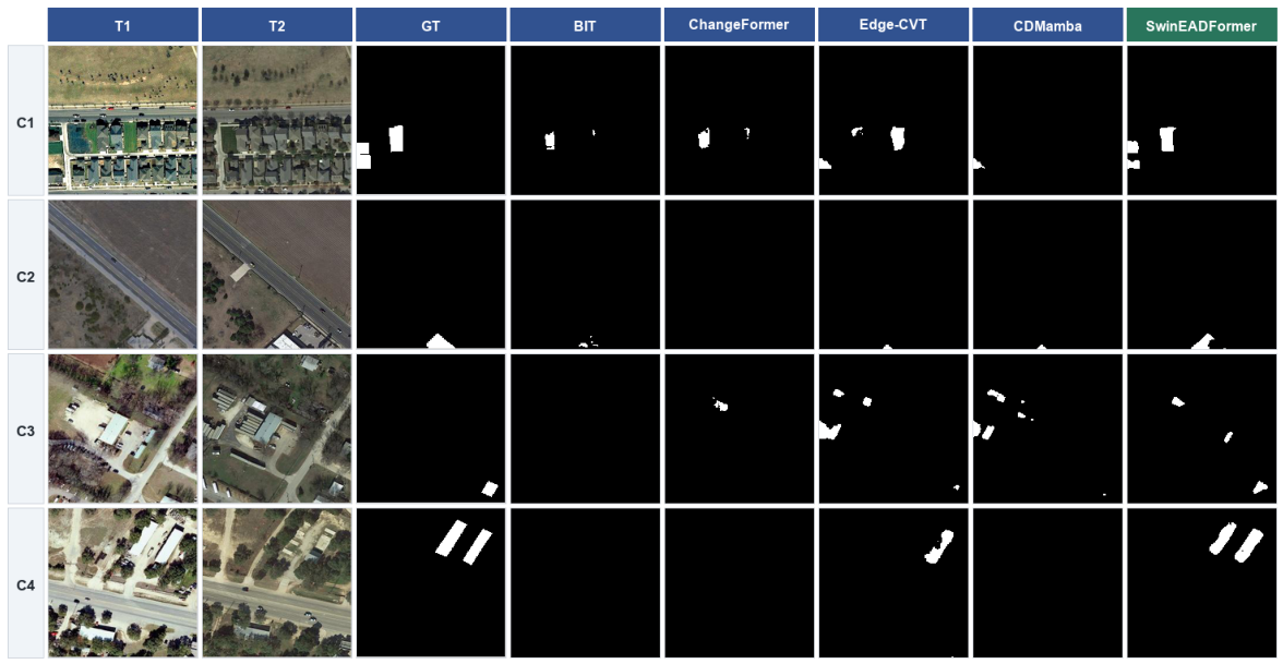
As shown in Figure 5, several competing methods miss narrow buildings, small objects, or parts of fragmented change regions, while others produce isolated false responses. SwinEADFormer yields more continuous predictions in these cases, consistent with its higher mean recall and F1 score.

Figure 6 shows missed and extra boundaries. SwinEADFormer recovers more complete contours in several illustrated cases, although false-positive and missed segments remain in heterogeneous backgrounds. It achieves the highest mean boundary F1 but not the best boundary IoU, indicating stronger tolerance-based contour recovery than strict boundary-band overlap.

4.4. Additional Dataset Evaluation and Efficiency Analysis

To evaluate performance beyond LEVIR-CD,

Table 5. Multi-seed comparison on the WHU-CD and SYSU-CD datasets. Results are reported as mean ± standard deviation over five random seeds and are expressed as percentages. The best mean value for each dataset is shown in bold.

Dataset	Method	Precision	Recall	F1	IoU	OA
WHU-CD	FCCDN	$74.32\pm 0.15$	$77.04\pm 0.21$	$75.66\pm 0.05$	$60.84\pm 0.07$	$97.03\pm 0.01$
	SNUNet-CD	$66.04\pm 0.18$	$\mathbf{82.20}\mathbf{\pm }\mathbf{0.24}$	$73.24\pm 0.13$	$57.78\pm 0.16$	$96.40\pm 0.02$
	Edge-CVT	$66.56\pm 0.17$	$77.81\pm 0.20$	$71.75\pm 0.12$	$55.94\pm 0.14$	$96.32\pm 0.02$
	CDMamba	$72.43\pm 0.14$	$77.44\pm 0.18$	$74.85\pm 0.14$	$59.81\pm 0.18$	$96.88\pm 0.02$
	BIT	$\mathbf{84.01}\mathbf{\pm }\mathbf{0.11}$	$61.67\pm 0.19$	$71.13\pm 0.14$	$55.19\pm 0.17$	$97.00\pm 0.01$
	ChangeFormer	$82.86\pm 0.10$	$70.87\pm 0.17$	$\mathbf{76.40}\mathbf{\pm }\mathbf{0.07}$	$\mathbf{61.81}\mathbf{\pm }\mathbf{0.09}$	$\mathbf{97.37}\mathbf{\pm }\mathbf{0.01}$
	SwinEADFormer	$76.66\pm 0.12$	$75.75\pm 0.16$	$76.20\pm 0.13$	$61.55\pm 0.17$	$97.16\pm 0.02$
SYSU-CD	FCCDN	$75.94\pm 0.14$	$76.97\pm 0.18$	$76.45\pm 0.11$	$61.88\pm 0.14$	$88.86\pm 0.05$
	SNUNet-CD	$80.04\pm 0.12$	$79.27\pm 0.16$	$79.65\pm 0.13$	$66.19\pm 0.18$	$90.48\pm 0.06$
	Edge-CVT	$78.97\pm 0.11$	$78.67\pm 0.15$	$78.82\pm 0.12$	$65.04\pm 0.17$	$90.06\pm 0.06$
	CDMamba	$79.32\pm 0.13$	$81.06\pm 0.17$	$80.18\pm 0.15$	$66.92\pm 0.20$	$90.58\pm 0.07$
	BIT	$80.96\pm 0.10$	$74.79\pm 0.18$	$77.75\pm 0.06$	$63.60\pm 0.09$	$89.94\pm 0.02$
	ChangeFormer	$80.47\pm 0.12$	$74.23\pm 0.20$	$77.22\pm 0.16$	$62.90\pm 0.21$	$89.71\pm 0.06$
	SwinEADFormer	$\mathbf{83.87}\mathbf{\pm }\mathbf{0.09}$	$\mathbf{83.39}\mathbf{\pm }\mathbf{0.12}$	$\mathbf{83.63}\mathbf{\pm }\mathbf{0.09}$	$\mathbf{71.86}\mathbf{\pm }\mathbf{0.13}$	$\mathbf{92.32}\mathbf{\pm }\mathbf{0.04}$

reports the results on WHU-CD and SYSU-CD. These datasets provide additional evaluation settings with different data distributions and change patterns. Each model is trained and tested separately on each dataset. This experiment evaluates within-dataset performance under different data distributions and does not evaluate cross-dataset transfer.

For efficiency analysis,

Table 6. Model complexity and runtime comparison at an input resolution of $256\times 256$.

Method	Params	FLOPs	Latency	FPS	Peak Mem.
	(M)	(G)	(ms)	(Image/s)	(GB)
FC-EF	1.95	21.37	2.00	499.79	0.08
FC-Siam-conc	2.44	34.05	3.28	304.89	0.12
FC-Siam-diff	1.95	28.01	2.83	353.77	0.11
BIT	12.40	21.65	12.36	80.89	0.08
Edge-CVT	7.27	58.77	5.70	175.33	0.14
CDMamba	20.19	164.96	16.33	61.23	0.28
ChangeFormer	41.03	234.56	19.73	50.68	0.45
SwinEADFormer	35.43	39.84	20.45	48.89	0.17

reports the number of parameters, FLOPs, latency, throughput, and peak GPU memory at an input resolution of $256\times 256$. All methods are profiled under the same hardware and software environment using a batch size of 1, 20 warm-up iterations, and 100 measured iterations.

Table 6 shows that SwinEADFormer requires 39.84 G FLOPs and 0.17 GB of peak GPU memory, both of which are lower than those of ChangeFormer and CDMamba. However, it contains 35.43 M parameters and has the highest measured latency and the lowest FPS among the compared methods. These measurements indicate moderate arithmetic complexity but limited wall-clock efficiency. Runtime is also affected by kernel efficiency, memory access, tensor operations, and attention implementation. Therefore, the reported measurements describe an accuracy–resource trade-off for the current implementation and hardware.

5. Discussion

The ablation results show the largest degradations when $\mathrm{\Phi }$ fusion is removed or bidirectional interaction is replaced with unidirectional interaction. The S3 difference representation provides direct mid-level change evidence, while the bidirectional EAD branches capture temporal discrepancies from both directions. $\mathrm{\Phi }$ fusion combines the interaction-aware discrepancy with direct difference features.

SwinEADFormer differs from Changer by applying an image-pair-specific edge–region–semantic router to S3 cross-temporal attention in both temporal directions. It differs from Edge-CVT in how edge information is used: the edge response forms one component of an image-pair-specific gate that directly modulates cross-temporal attention outputs. The complete pipeline links direct difference evidence, spatially modulated cross-temporal attention, and bidirectional discrepancy fusion.

The ablation results empirically support the proposed interaction-evidence organization. Removing $\mathrm{\Phi }$ fusion causes the largest overall degradation, indicating that interaction-derived features alone are insufficient and that learned and direct S3 difference evidence remains important. Replacing bidirectional interaction with a unidirectional variant also reduces region-level and boundary-level performance, supporting the explicit modeling of directional interaction discrepancy. Router-related variants produce smaller but consistent changes, showing that the router provides secondary spatial modulation rather than acting as the dominant source of improvement. These findings support the proposed architecture as a task-driven inductive bias for sparse building change detection. They provide empirical evidence under the evaluated datasets and protocols but do not constitute a formal theoretical guarantee.

The quantitative and qualitative results indicate that SwinEADFormer favors complete recovery of changed-building regions. The method achieves competitive F1-score and IoU values across the evaluated datasets. On LEVIR-CD, it obtains the highest mean B-recall and B-F1 among the compared methods. However, the improvements over strong recent baselines are moderate. The method does not achieve the best precision or boundary IoU in every setting. This suggests a trade-off between region completeness, false-alarm control, and strict boundary overlap. Background structures with building-like textures, local radiometric differences, and imperfect boundary alignment remain important sources of error.

The conclusions of this study are limited to co-registered high-resolution optical change detection under the evaluated datasets and protocols. LEVIR-CD and WHU-CD provide building-focused settings, whereas SYSU-CD includes a broader range of binary changes. Future work will examine multispectral, SAR, cross-sensor, and seasonally diverse image pairs, with particular attention to sensor adaptation and cross-modal alignment.

6. Conclusions

This paper presented SwinEADFormer, a difference-conditioned and discrepancy-aware cross-temporal interaction framework for binary building change detection. An image-pair-specific router modulates S3 attention outputs before residual addition while preserving the original query path. The model explicitly represents the discrepancy between the two temporal interaction directions and fuses it with learned and direct S3 difference evidence. Therefore, the resulting representation retains both interaction-derived evidence and direct temporal differences.

Experiments on LEVIR-CD, WHU-CD, and SYSU-CD show competitive region-level performance against representative baselines. On LEVIR-CD, SwinEADFormer achieves the highest mean B-recall and B-F1. Five-seed ablations show clearer gains from $\mathrm{\Phi }$ fusion and bidirectional interaction, while router-related variants produce smaller mean changes. Therefore, the router contributes modest spatial guidance to cross-temporal interaction.

The current evaluation is limited to co-registered high-resolution optical change detection datasets. LEVIR-CD and WHU-CD are building-focused, whereas SYSU-CD includes broader binary changes. The experiments do not establish performance on SAR, multispectral, cross-sensor, or strongly seasonal image pairs. Future work will examine sensor adaptation, cross-modal alignment, false-positive suppression, and more efficient router designs.

References

- Singh, A. Digital change detection techniques using remotely-sensed data. Int. J. Remote Sens. 1989, 10, 989–1003. [Google Scholar] [CrossRef] [Scilit]
- Lu, D.; Mausel, P.; Brondizio, E.; Moran, E. Change detection techniques. Int. J. Remote Sens. 2004, 25, 2365–2401. [Google Scholar] [CrossRef] [Scilit]
- Coppin, P.; Jonckheere, I.; Nackaerts, K.; Muys, B.; Lambin, E. Digital change detection methods in ecosystem monitoring: A review. Int. J. Remote Sens. 2004, 25, 1565–1596. [Google Scholar] [CrossRef] [Scilit]
- Daudt, R.C.; Le Saux, B.; Boulch, A. Fully convolutional Siamese networks for change detection. In Proceedings of the 25th IEEE International Conference on Image Processing (ICIP), Athens, Greece, 7–10 October 2018; pp. 4063–4067. [Google Scholar] [CrossRef] [Scilit]
- Zhan, Y.; Fu, K.; Yan, M.; Sun, X.; Wang, H.; Qiu, X. Change detection based on deep Siamese convolutional network for optical aerial images. IEEE Geosci. Remote Sens. Lett. 2017, 14, 1845–1849. [Google Scholar] [CrossRef] [Scilit]
- Zhang, C.; Yue, P.; Tapete, D.; Jiang, L.; Shangguan, B.; Huang, L.; Liu, G. A deeply supervised image fusion network for change detection in high resolution bi-temporal remote sensing images. ISPRS J. Photogramm. Remote Sens. 2020, 166, 183–200. [Google Scholar] [CrossRef] [Scilit]
- Fang, S.; Li, K.; Shao, J.; Li, Z. SNUNet-CD: A densely connected Siamese network for change detection of VHR images. IEEE Geosci. Remote Sens. Lett. 2022, 19, 8007805. [Google Scholar] [CrossRef] [Scilit]
- Vaswani, A.; Shazeer, N.; Parmar, N.; Uszkoreit, J.; Jones, L.; Gomez, A.N.; Kaiser, Ł.; Polosukhin, I. Attention is all you need. In Proceedings of the Advances in Neural Information Processing Systems, Long Beach, CA, USA, 4–9 December 2017; Volume 30, pp. 5998–6008. [Google Scholar]
- Dosovitskiy, A.; Beyer, L.; Kolesnikov, A.; Weissenborn, D.; Zhai, X.; Unterthiner, T.; Dehghani, M.; Minderer, M.; Heigold, G.; Gelly, S.; et al. An image is worth 16×16 words: Transformers for image recognition at scale. In Proceedings of the International Conference on Learning Representations, Virtual Event, 3–7 May 2021. [Google Scholar]
- Liu, Z.; Lin, Y.; Cao, Y.; Hu, H.; Wei, Y.; Zhang, Z. Swin Transformer: Hierarchical vision Transformer using shifted windows. In Proceedings of the IEEE/CVF International Conference on Computer Vision (ICCV), Montreal, QC, Canada, 10–17 October 2021; pp. 9992–10002. [Google Scholar] [CrossRef] [Scilit]
- Chen, H.; Qi, Z.; Shi, Z. Remote sensing image change detection with Transformers. IEEE Trans. Geosci. Remote Sens. 2022, 60, 5607514. [Google Scholar] [CrossRef] [Scilit]
- Bandara, W.G.C.; Patel, V.M. A Transformer-based Siamese network for change detection. In Proceedings of the 2022 IEEE International Geoscience and Remote Sensing Symposium, Kuala Lumpur, Malaysia, 17–22 July 2022; pp. 207–210. [Google Scholar] [CrossRef] [Scilit]
- Saha, S.; Bovolo, F.; Bruzzone, L. Unsupervised deep change vector analysis for multiple-change detection in VHR images. IEEE Trans. Geosci. Remote Sens. 2019, 57, 3677–3693. [Google Scholar] [CrossRef] [Scilit]
- Zhu, X.X.; Tuia, D.; Mou, L.; Xia, G.-S.; Zhang, L.; Xu, F. Deep learning in remote sensing: A comprehensive review and list of resources. IEEE Geosci. Remote Sens. Mag. 2017, 5, 8–36. [Google Scholar] [CrossRef] [Scilit]
- Ma, L.; Liu, Y.; Zhang, X.; Ye, Y.; Yin, G.; Johnson, B.A. Deep learning in remote sensing applications: A meta-analysis and review. ISPRS J. Photogramm. Remote Sens. 2019, 152, 166–177. [Google Scholar] [CrossRef] [Scilit]
- Shafique, A.; Cao, G.; Khan, Z.; Asad, M.; Aslam, M. Deep learning-based change detection in remote sensing images: A review. Remote Sens. 2022, 14, 871. [Google Scholar] [CrossRef] [Scilit]
- Parelius, E.J. A review of deep-learning methods for change detection in multispectral remote sensing images. Remote Sens. 2023, 15, 2092. [Google Scholar] [CrossRef] [Scilit]
- Long, J.; Shelhamer, E.; Darrell, T. Fully convolutional networks for semantic segmentation. In Proceedings of the IEEE Conference on Computer Vision and Pattern Recognition (CVPR), Boston, MA, USA, 7–12 June 2015; pp. 3431–3440. [Google Scholar] [CrossRef] [Scilit]
- Ronneberger, O.; Fischer, P.; Brox, T. U-Net: Convolutional networks for biomedical image segmentation. In Proceedings of the Medical Image Computing and Computer-Assisted Intervention; Springer: Cham, Switzerland, 2015; pp. 234–241. [Google Scholar] [CrossRef] [Scilit]
- Badrinarayanan, V.; Kendall, A.; Cipolla, R. SegNet: A deep convolutional encoder-decoder architecture for image segmentation. IEEE Trans. Pattern Anal. Mach. Intell. 2017, 39, 2481–2495. [Google Scholar] [CrossRef] [Scilit] [PubMed]
- He, K.; Zhang, X.; Ren, S.; Sun, J. Deep residual learning for image recognition. In Proceedings of the IEEE Conference on Computer Vision and Pattern Recognition (CVPR), Las Vegas, NV, USA, 27–30 June 2016; pp. 770–778. [Google Scholar] [CrossRef] [Scilit]
- Huang, G.; Liu, Z.; Van Der Maaten, L.; Weinberger, K.Q. Densely connected convolutional networks. In Proceedings of the IEEE Conference on Computer Vision and Pattern Recognition (CVPR), Honolulu, HI, USA, 21–26 July 2017; pp. 2261–2269. [Google Scholar] [CrossRef] [Scilit]
- Lin, T.Y.; Dollar, P.; Girshick, R.; He, K.; Hariharan, B.; Belongie, S. Feature pyramid networks for object detection. In Proceedings of the IEEE Conference on Computer Vision and Pattern Recognition (CVPR), Honolulu, HI, USA, 21–26 July 2017; pp. 936–944. [Google Scholar] [CrossRef] [Scilit]
- Chen, H.; Li, W.; Chen, S.; Shi, Z. Semantic-aware dense representation learning for remote sensing image change detection. IEEE Trans. Geosci. Remote Sens. 2022, 60, 5630018. [Google Scholar] [CrossRef] [Scilit]
- Mou, L.; Bruzzone, L.; Zhu, X.X. Learning spectral-spatial-temporal features via a recurrent convolutional neural network for change detection in multispectral imagery. IEEE Trans. Geosci. Remote Sens. 2019, 57, 924–935. [Google Scholar] [CrossRef] [Scilit]
- Peng, D.; Zhang, Y.; Guan, H. End-to-end change detection for high resolution satellite images using improved UNet++. Remote Sens. 2019, 11, 1382. [Google Scholar] [CrossRef] [Scilit]
- Chen, J.; Yuan, Z.; Peng, J.; Chen, L.; Huang, H.; Zhu, J. DASNet: Dual attentive fully convolutional Siamese networks for change detection in high-resolution satellite images. IEEE J. Sel. Top. Appl. Earth Obs. Remote Sens. 2021, 14, 1194–1206. [Google Scholar] [CrossRef] [Scilit]
- Chen, P.; Zhang, B.; Hong, D.; Chen, Z.; Yang, X.; Li, B. FCCDN: Feature constraint network for VHR image change detection. ISPRS J. Photogramm. Remote Sens. 2022, 187, 101–119. [Google Scholar] [CrossRef] [Scilit]
- Shi, Q.; Liu, M.; Li, S.; Liu, X.; Wang, F.; Zhang, L. A deeply supervised attention metric-based network and an open aerial image dataset for remote sensing change detection. IEEE Trans. Geosci. Remote Sens. 2022, 60, 5604816. [Google Scholar] [CrossRef] [Scilit]
- Fang, S.; Li, K.; Li, Z. Changer: Feature interaction is what you need for change detection. IEEE Trans. Geosci. Remote Sens. 2023, 61, 5610111. [Google Scholar] [CrossRef] [Scilit]
- Noman, M.; Fiaz, M.; Cholakkal, H.; Narayan, S.; Anwer, R.M.; Khan, S. Remote sensing change detection with Transformers trained from scratch. IEEE Trans. Geosci. Remote Sens. 2024, 62, 4704214. [Google Scholar] [CrossRef] [Scilit]
- Carion, N.; Massa, F.; Synnaeve, G.; Usunier, N.; Kirillov, A.; Zagoruyko, S. End-to-end object detection with Transformers. In Proceedings of the Computer Vision–ECCV 2020; Springer: Cham, Switzerland, 2020; pp. 213–229. [Google Scholar] [CrossRef] [Scilit]
- Zheng, S.; Lu, J.; Zhao, H.; Zhu, X.; Luo, Z.; Wang, Y. Rethinking semantic segmentation from a sequence-to-sequence perspective with Transformers. In Proceedings of the IEEE/CVF Conference on Computer Vision and Pattern Recognition (CVPR), Nashville, TN, USA, 20–25 June 2021; pp. 6877–6886. [Google Scholar] [CrossRef] [Scilit]
- Xie, E.; Wang, W.; Yu, Z.; Anandkumar, A.; Alvarez, J.M.; Luo, P. SegFormer: Simple and efficient design for semantic segmentation with Transformers. In Proceedings of the Advances in Neural Information Processing Systems, Online, 6–14 December 2021; Volume 34, pp. 12077–12090. [Google Scholar]
- Zhang, C.; Wang, L.; Cheng, S.; Li, Y. SwinSUNet: Pure Transformer network for remote sensing image change detection. IEEE Trans. Geosci. Remote Sens. 2022, 60, 5224713. [Google Scholar] [CrossRef] [Scilit]
- Zhang, K.; Zhao, X.; Zhang, F.; Ding, L.; Sun, J.; Bruzzone, L. Relation changes matter: Cross-temporal difference Transformer for change detection in remote sensing images. IEEE Trans. Geosci. Remote Sens. 2023, 61, 5611615. [Google Scholar] [CrossRef] [Scilit]
- Naveed, H.; Zeng, X.; Bryson, M.; Mehrseresht, N. Multi-Receptive Field Ensemble with Cross-Entropy Masking for Class Imbalance in Remote Sensing Change Detection. arXiv 2025, arXiv:2508.10568. [Google Scholar] [CrossRef] [Scilit]
- Liu, Y.; Yang, Y.; Li, J.; Tao, J.; Li, R.; Wang, X.; Zhu, M.; Cheng, J. LG-CD: Enhancing language-guided change detection through SAM2 adaptation. arXiv 2025, arXiv:2509.21894. [Google Scholar] [CrossRef] [Scilit]
- Madani, S.; Chellappa, R.; Patel, V.M. DiffRegCD: Integrated registration and change detection with diffusion features. arXiv 2025, arXiv:2511.07935. [Google Scholar] [CrossRef] [Scilit]
- Otsu, N. A threshold selection method from gray-level histograms. IEEE Trans. Syst. Man Cybern. 1979, 9, 62–66. [Google Scholar] [CrossRef] [Scilit]
- Bruzzone, L.; Prieto, D.F. Automatic analysis of the difference image for unsupervised change detection. IEEE Trans. Geosci. Remote Sens. 2000, 38, 1171–1182. [Google Scholar] [CrossRef] [Scilit]
- Celik, T. Unsupervised change detection in satellite images using principal component analysis and k-means clustering. IEEE Geosci. Remote Sens. Lett. 2009, 6, 772–776. [Google Scholar] [CrossRef] [Scilit]
- Kervadec, H.; Bouchtiba, J.; Desrosiers, C.; Granger, E.; Dolz, J.; Ben Ayed, I. Boundary loss for highly unbalanced segmentation. Med. Image Anal. 2021, 67, 101851. [Google Scholar] [CrossRef] [Scilit] [PubMed]
- Cheng, B.; Girshick, R.; Dollar, P.; Berg, A.C.; Kirillov, A. Boundary IoU: Improving object-centric image segmentation evaluation. In Proceedings of the IEEE/CVF Conference on Computer Vision and Pattern Recognition (CVPR), Nashville, TN, USA, 20–25 June 2021; pp. 15329–15337. [Google Scholar] [CrossRef] [Scilit]
- Yang, B.; Huang, Y.; Su, X.; Guo, H. MAEANet: Multiscale attention and edge-aware Siamese network for building change detection in high-resolution remote sensing images. Remote Sens. 2022, 14, 4895. [Google Scholar] [CrossRef] [Scilit]
- Holail, S.; Saleh, T.; Xiao, X.; Zahran, M.; Xia, G.S.; Li, D. Edge-CVT: Edge-informed CNN and vision transformer for building change detection in satellite imagery. ISPRS J. Photogramm. Remote Sens. 2025, 227, 48–68. [Google Scholar] [CrossRef] [Scilit]
- Li, Y.C.; Lei, S.; Zhao, Y.T.; Li, H.C.; Li, J.; Plaza, A.J. SAM-Based building change detection with distribution-aware Fourier adaptation and edge-constrained warping. IEEE Trans. Geosci. Remote Sens. 2025, 63, 5651114. [Google Scholar] [CrossRef] [Scilit]
- Lin, T.Y.; Goyal, P.; Girshick, R.; He, K.; Dollar, P. Focal loss for dense object detection. In Proceedings of the IEEE International Conference on Computer Vision (ICCV), Venice, Italy, 22–29 October 2017; pp. 2999–3007. [Google Scholar] [CrossRef] [Scilit]
- Milletari, F.; Navab, N.; Ahmadi, S.A. V-Net: Fully convolutional neural networks for volumetric medical image segmentation. In Proceedings of the Fourth International Conference on 3D Vision (3DV), Stanford, CA, USA, 25–28 October 2016; pp. 565–571. [Google Scholar] [CrossRef] [Scilit]
- Chen, H.; Shi, Z. A spatial-temporal attention-based method and a new dataset for remote sensing image change detection. Remote Sens. 2020, 12, 1662. [Google Scholar] [CrossRef] [Scilit]
- Ji, S.; Wei, S.; Lu, M. Fully convolutional networks for multisource building extraction from an open aerial and satellite imagery data set. IEEE Trans. Geosci. Remote Sens. 2019, 57, 574–586. [Google Scholar] [CrossRef] [Scilit]
- Loshchilov, I.; Hutter, F. Decoupled weight decay regularization. In Proceedings of the International Conference on Learning Representations, New Orleans, LA, USA, 6–9 May 2019. [Google Scholar]
- Chen, H.; Song, J.; Han, C.; Xia, J.; Yokoya, N. ChangeMamba: Remote sensing change detection with spatiotemporal state space model. IEEE Trans. Geosci. Remote Sens. 2024, 62, 4409720. [Google Scholar] [CrossRef] [Scilit]
- Zhang, H.; Chen, K.; Liu, C.; Chen, H.; Zou, Z.; Shi, Z. CDMamba: Incorporating local clues into Mamba for remote sensing image binary change detection. arXiv 2024, arXiv:2406.04207. [Google Scholar] [CrossRef] [Scilit]
Figure 1.
Overall architecture of the proposed SwinEADFormer. The model extracts hierarchical bitemporal features with a shared Swin-Tiny encoder, constructs a stage-3 (S3) difference representation, generates an image-pair-specific edge–region–semantic router, performs bidirectional edge-aware dynamic (EAD) interaction, and decodes the fused change representation into the final prediction. Here, S3 denotes stage-3 encoder features at input resolution; EAD denotes edge-aware dynamic interaction; denotes the feature fusion operator; ⊙ denotes element-wise multiplication; and , , and denote edge, region, and semantic cues, respectively.