


Highlights
What are the main findings?
- The LMT-Random Subspace ensemble achieves the best spatial cross-validation AUC (0.954 ± 0.019), outperforming LMT (0.925 ± 0.023) and AdaBoost-LMT (0.934 ± 0.021).
- The DeLong test confirms that the superiority of LMT-RSM over LMT is statistically significant (p < 0.0001).
- The LMT-RSM model captures 95.98% of landslides in very high and high susceptibility zones.
What are the implications of the main findings?
- An adaptive slope-unit optimization framework is proposed using the composite index S to balance terrain subdivision quality and model predictive performance.
- The framework integrates optimized slope units, ensemble learning, and spatially explicit validation for robust LSM.
Abstract
Landslide susceptibility mapping (LSM) serves as a fundamental technical support for geohazard prevention and mitigation across mountainous terrains. This research constructs a multi-scale terrain unit integrated modeling framework targeting complex mountainous geomorphic settings, taking Zhenping County as the research object. Multi-resolution digital elevation model (DEM) datasets, multi-source satellite remote sensing imagery (GF-2), geological vector datasets and hydrological survey data are jointly adopted as the basic data source. The r.slopeunits module embedded in GRASS GIS is utilized to automatically segment slope units, and a comprehensive composite index S, coupling slope partition quality indicator F and model prediction accuracy metric R, is proposed to adaptively optimize two critical slope-unit hyperparameters: circular variance (c) and minimum unit area (a). Four DEM spatial resolutions (15 m, 25 m, 50 m, 100 m) are systematically calibrated with 42 groups of c–a parameter combinations to screen out the optimal slope-unit segmentation scheme (c = 0.1, a = 200,000 m2). Twelve landslide predisposing covariates covering topography, hydrology, lithology, human engineering activities and land cover are selected after multicollinearity diagnosis via Variance Inflation Factor and mean utility factor contribution evaluation. Logistic regression tree (LMT), LMT-Adaboost and LMT-Random Subspace are compared by random cross-validation and spatial block cross-validation. Parameter sensitivity analysis is further carried out to quantify the stability of model outputs against DEM resolution and slope-unit parameter perturbations. The LMT-RSM ensemble achieved the highest spatial cross-validation AUC (0.954 ± 0.019), outperforming LMT (0.925 ± 0.023) and AdaBoost-LMT (0.934 ± 0.021). The DeLong test confirmed that LMT-RSM’s superiority over LMT is statistically significant (p < 0.0001). The proportion of landslides in the very high and high susceptibility zones under the LMT-RSM model reached 95.98%, demonstrating relatively excellent spatial discrimination. This study provides an operational framework combining optimized slope units, ensemble learning, and spatially explicit validation for robust LSM in complex terrain, and offers a reproducible technical pathway for landslide risk prevention in mountainous regions.
1. Introduction
Landslides impose a huge socio-economic burden and rank as the seventh deadliest natural disaster globally, as well as the fourth in terms of the number of people affected worldwide [1], causing significant casualties and economic losses [2,3], especially in mountainous and tectonically active regions where the vulnerability of infrastructure and human activities can exacerbate the disaster impact [4]. The Eurasian, Pacific and Indian tectonic junction zones are characterized by west-high–east-low terrain frameworks, with two-thirds of their area being mountainous with frequent crustal movements, making these areas prone to geological disasters [5]. Zhenping County in China has a fragile geological environment and a long history of landslides, making it a region prone to landslide disasters. Hence, Zhenping County has been selected as the study region to implement a full-scale and high-precision landslide susceptibility assessment [6].
Over the past decades, a wide range of methods have been developed for landslide susceptibility mapping (LSM), which can be broadly categorized into statistical models and machine learning approaches. Currently, widely adopted statistical paradigms include the evidence belief function (EBF) [7,8], analytical hierarchy process (AHP) [9,10,11], statistical index (SI) [12,13], weight of evidence (WOE) [14,15,16] and logistic regression (LR) [17,18,19]. The FR-EBF model’s multiplicative integration addresses the limitations of independent models in heterogeneous terrains, providing a transferable framework for integrating geostatistical and machine learning methods [7]. The FR-AHP model combines landslide statistical inventory analysis with MCDM to generate high-resolution LSMs for the Aqra region in northern Iraqi mountains, reducing the destructive impact of regional landslides [9]. The landslide susceptibility mapping in Yanchuan, China, using WOE, LR, NB, and ADTree models, demonstrated the competitiveness of traditional models in machine learning [17]. These statistical methods are valued for their simplicity and interpretability; however, they generally presuppose linear correlations or conditional independence between variables, limiting their capacity to characterize intricate nonlinear interactions between landslide impact factors and slide events. Machine learning approaches, in contrast, can capture nonlinear interactions but are prone to overfitting and require careful tuning and factor selection; common machine learning methods include Adaboost [20,21], artificial neural network (ANN) [22,23], support vector machine (SVM) [24,25,26], maximum entropy (MaxEnt) [27,28,29], logistic model tree (LMT) [30,31], Random Subspace Methods (RSMs) [32,33], and random forest (RF) [24,34]. The RF model outperforms SVM and XGBoost models in predicting landslide susceptibility due to its ability to retain input parameters and handle large datasets flexibly [24]. The uncertainty in selecting landslide-inducing factors significantly affects landslide susceptibility prediction. Identifying the optimal selection and combination methods can lead to efficient LSP modeling [35]. The RF-Adaboost model enhances prediction accuracy and robustness to input data variations by integrating data from different sources, reducing the model’s dependence on individual features [20]. Recent studies have improved prediction accuracy through methods such as FR-EBF fusion [7], PSO-ANN optimization [22], RF-Adaboost integration [20] and SVM-GOA integration [36]. The LWL-RS-CDT integrated model achieved an AUC value as high as 0.974 ± 0.977 [37]. Although these integrated models have high predictive performance, the mechanism by which they compensate for terrain-related biases has received little research, and most of these ensemble models are evaluated using regular grids [38,39,40,41], or hydrological analysis tools [42,43,44,45,46,47]. These methods have advantages in simplifying the calculation process and facilitating automated processing. However, regular grids may cut through the physical boundaries of natural slopes, resulting in high internal terrain heterogeneity within the units; traditional hydrological units focus on catchment area division and are unable to reflect the geometric morphological features required for slope stability analysis (such as slope consistency and sliding direction).
In response to these limitations, automated terrain segmentation has advanced, with Alvioli et al. developing r.slopeunits for reproducible slope-unit delineation [48]. Subsequent studies show that slope-unit scale affects sample distribution and model performance, with finer units not necessarily better [49,50], and the number of units conditioning factor contributions [51]. Spatial heterogeneity has been addressed via geographically weighted random forest and partitioning frameworks [52]. While individual advances have been made in terrain segmentation and ensemble modeling separately, the synergistic integration of adaptive slope unit optimization with ensemble learning and the critical evaluation of how terrain partitioning choices affect ensemble model behavior has not been systematically investigated.
Based on the above research, it is likely that the unoptimized spatial unit scheme and single modeling framework are the main factors restricting the prediction accuracy and robustness of current LSM models. To address this gap, we propose a multi-scale terrain unit-driven framework for landslide susceptibility in complex mountainous areas. Its novelty lies in (1) adaptive optimization of slope-unit parameters via r.slopeunits with multi-resolution DEM, overcoming fixed-parameter limitations; (2) systematic comparison of LMT, LMT-RSM, and LMT-Adaboost within unified slope units, revealing ensemble-terrain interactions; and (3) an integrated system jointly optimizing units, factors, and models—an approach not yet systematically implemented in such terrain settings.
This paper proposes a multi-scale terrain unit-driven integrated modeling method for the landslide spatial characteristics in complex terrain areas. Based on the GrassGIS software (version 7.8), the r.slopeunits module is integrated, and multi-resolution DEM data are used to automatically partition slope units. The adaptive optimization for morphological parameters of slope units (c = 0.1, a = 2 × 10⁵ m2) is realized. Then, the multicollinearity test and related attribute evaluation are used to optimize the landslide conditioning factors. Furthermore, the performance of LMT, LMT-RSM, and LMT-Adaboost models in landslide susceptibility modeling is compared. Finally, the ROC, Kappa coefficient, and AUC parameters are used to optimize the model and achieve the optimization of the landslide susceptibility evaluation system. The selected LMT-RSM integrated model in this paper has a high AUC prediction value of 0.994, effectively solving the bottleneck problems of poor terrain adaptability and insufficient prediction ability of traditional models, providing a new technical path for landslide risk prevention and control in mountainous regions.
2. Study Area and Data Used
2.1. General Situation of the Study Area
Zhenping County is geographically positioned in the southern region of Shaanxi Province, China, on the northern foothills of the Daba Mountains. It covers a total area of 1503 square kilometers. The terrain within the county is higher in the southwest and lower in the northeast, with a maximum elevation difference of 2417 m (the highest point is 2917 m and the lowest point is 500 m), making it one of the regions with the most dramatic topography in Shaanxi Province (Figure 1).
Figure 1.
Study area and landslide inventory map.
The county’s landscape is dominated by medium mountains (1000–1500 m) and high medium mountains (>1500 m), accounting for over 80% of the area. Low-altitude mountainous terrains dominate the middle and lower reaches of the Nanjiang River, with many areas covered in gravel deposits. Medium mountains have deep valleys and steep slopes, and landslides occur frequently. High medium mountains include the main ridge of the Daba Mountains, featuring numerous cliffs and precipices. The county’s entire river system is incorporated into the Han River hydrological network. The main river, the Nanjiang River, is 107 km long, and its basin covers the entire county. Twenty-seven tributaries form a dense river network. Due to the influence of the terrain, the rivers are short (<30 km), with large drops (gradient of 15‰) forming V-shaped canyons (riverbed width 10–50 m, bank height over 200 m). During the flood season, 75% of the annual runoff occurs, and the peak flow carries sand and stones at a speed of 3–5 m per second.
2.2. Landslide Inventory Map
Through historical data, high-resolution remote sensing images (GF-2 with 2 m pan-sharpened multispectral imagery and Sentinel-2 with 10 m resolution), and extensive field investigations, a total of 140 landslides were identified. Among them, 97.14% were accumulation-layer landslides and 85% were shallow landslides, mainly distributed in a band-like pattern along highways and gullies. The scale of landslides is mainly small (85%), with strong activity and great hazard.
To ensure the robustness and objectivity of the model evaluation, a total of 140 landslide polygons were randomly split at the polygon scale into a 70% training dataset and a 30% validation dataset. When selecting non-slide samples, a spatial constraint sampling strategy was adopted to reduce potential spatial sampling bias. Specifically, a 200 m buffer zone was delineated around each landslide polygon, and no non-slide points were selected within this area to avoid sampling in areas prone to landslides. In the remaining stable areas, stratified random sampling was used, and the samples were matched at a 1:1 ratio with the landslide samples, forming the training set and validation set containing the data of landslide points [3,53].
Furthermore, to account for spatial dependence in the random split procedure, a spatial cross-validation strategy was implemented. The study area was partitioned into spatially contiguous blocks, ensuring that training and validation samples were separated by at least the spatial autocorrelation range of the landslide conditioning factors. This approach mitigates the potential overestimation of predictive performance that could arise from spatial autocorrelation between training and validation datasets [54].
2.3. Landslide Conditioning Factors
Landslide disasters are complex products of the synergistic effect of natural and human factors, and their accurate prediction requires the systematic integration of multi-dimensional disaster-causing factors. The selection of conditioning factors in this study was guided by a threefold rationale: (1) their well-established mechanistic roles in landslide initiation, as documented in the literature; (2) their proven effectiveness in similar geomorphic and climatic settings; (3) their complementary contributions to cover the four principal controlling dimensions. Based on previous studies, four factors, namely, topography, geology, hydrology and land cover, are generally adopted to assess landslide susceptibility [35,54,55]. In this study, 12 conditioning factors (slope, aspect, elevation, plane curvature, profile curvature, topographic moisture index, lithology, distance to faults, NDVI, distance to rivers, distance to roads, and land-use type) were selected as the basis for the quantitative evaluation of landslides (Table 1, Figure 2) [56,57,58,59]. All factor layers were resampled to 15 m resolution and projected to CGCS2000. Zonal statistics aggregated pixel values to slope units: continuous factors (slope, elevation, plan curvature, profile curvature, TWI, NDVI, and the three distance metrics) were averaged, while categorical factors (aspect, lithology, land use) were assigned the modal class. Table 1 lists data sources, original resolutions, and aggregation methods.
Table 1.
Data sources, original resolutions, and aggregation methods.
Figure 2.
Landslide conditioning factors with 25 m resolution: (a) slope angle; (b) slope aspect; (c) elevation; (d) profile curvature; (e) plan curvature; (f) TWI; (g) distance to rivers; (h) distance to roads; (i) distance to faults; (j) land use; (k) lithology; (l) NDVI.
- (1)
- Slope angle
Slope angle, defined as the inclination between the terrain surface and the horizontal plane, reflects the degree of topographic steepness. As a critical influencing factor of slope stability [60,61], it dominates the internal stress distribution of slope masses and has a direct correlation with the occurrence of soil sliding failures [62]. The terrain slope of the study area is distributed between 0° and 60°, and generally shows a normal distribution trend. The number of grid points on both sides gradually decreases, with 30° as the center [63].
- (2)
- Slope aspect
The slope aspect is the direction of the projection of the normal of the slope surface on the horizontal plane [64]. The terrain aspect determines the quantity of solar irradiation on the land surface, exerting subsequent impacts on evaporation rates, weathering progress, vegetation cover and slope erosion processes, and further causing differences in slope stability [65]. This article classifies the slope aspects into nine categories, namely, flat land (−1), northward (337.5–360°, 0–22.5°), northeastward (22.5–67.5°), eastward (67.5–112.5°), southeastward (112.5–157.5°), southward (157.5–202.5°), southwest (202.5–247.5°), west (247.5–292.5°) and northwest (292.5–337.5°). Flat land occupies an extremely tiny proportion of the study area, merely making up less than 0.01% of the total territory, while the proportions of the other slopes are all greater than 10%. The overall differences are relatively small.
- (3)
- Elevation
Topographic elevation denotes the vertical height of a specific point against the standard datum surface [66,67]. Elevation data were extracted directly from the DEM, which was derived from stereo-optical remote sensing (GF-7 or ALOS PALSAR DEM). The elevation of the study area is distributed between 547 and 2911 m, concentrated between 1200 and 1800 m, and decreases on both sides with 1500 m as the boundary.
- (4)
- Plan curvature
Used to reflect horizontal surface distortion, plan curvature illustrates how severely contour lines bend at corresponding locations [60,68]. According to the curvature of the plane, slopes can be classified into inward shape (<0), outward shape (>0) or straight shape (=0). The planar curvature of the study area is mainly distributed between −5 and 5, and is concentrated between −1 and 1.
- (5)
- Profile curvature
This index reflects the vertical change rate of surface elevation and depicts the undulating bending status of terrain along the slope aspect [11,69]. According to profile curvature, slopes can be classified into concave (<0), convex (>0) and straight (=0) shapes. The curvature of the cross-section in the study area is mainly distributed between −5 and 5, and is concentrated between −1 and 1.
- (6)
- TWI
The topographic moisture index describes the influence of terrain on the location and scale of the saturated source area of runoff generation [55], and is calculated from the DEM (a remote sensing product) using the following formula:
In the formula, As represents the specific catchment area of each unit, and β represents the slope gradient of the terrain at a certain elevation. The topographic moisture index of the study area is mainly distributed between 0 and 7, with the highest distribution around 1.8. After that, the distribution quantity gradually decreases.
- (7)
- Lithology
The lithology of the strata in this study area is classified into 10 categories (Table 2). The lithology of the strata in the 7th category is mainly distributed, followed by the 6th category, then the 2nd, 8th and 9th categories, and the rest are distributed less frequently.
Table 2.
Stratigraphic lithological classification.
- (8)
- Distance to faults
The evolution of regional landforms is partially governed by faults, which also alter the stress distribution of rock and soil bodies. Meanwhile, fault planes and fractured zones create structurally weak interfaces inside rock masses, rendering these areas susceptible to sliding failures [70]. There are many faults in the study area, and the distance between each point and the faults is within 7000 m. Moreover, there are more grid points closer to the faults and fewer grid points farther away from them.
- (9)
- NDVI
The Normalized Difference Vegetation Index (NDVI) quantifies the coverage extent and density of vegetation derived from remote sensing imagery [71,72], and is directly computed from Sentinel-2 or Landsat multispectral bands using the following formula:
where R and IR represent the red and near-infrared bands, respectively.
Negative NDVI values correspond to water bodies or snow-covered regions, whereas positive values signify vegetated surfaces. Larger NDVI readings represent denser vegetation coverage across the terrain. In the study area, the NDVI mainly ranges from 0 to 0.5, with the most frequent distribution around 0.4. The number of grid points decreases gradually to the left, while there are fewer grid points to the right.
- (10)
- Distance to rivers
The role of surface water is manifested in the erosion of riverbanks by surface runoff, which increases the height and steepness of riverbank slopes, erodes the foot of the slope, weakens the slope’s supportive capacity, and leads to a decrease in slope stability and the occurrence of landslides and collapses [73]. There are many rivers in the study area, and the distance between each point and the rivers is within 2000 m. There are more grid points closer to the rivers and fewer grid points farther away from them.
- (11)
- Distance to roads
Restricted by complex topographic conditions, local road construction necessitates mountain excavation, resulting in numerous steep slopes and cliffs. The foot of the slope is exposed to the air, and slope instability is common, causing numerous geological hazard points to be distributed along the roads, representing the dominant distribution characteristic of local geological disasters [74,75]. There are few national and provincial roads in the study area, and the distance between each point and the roads can reach up to 13,000 m. Areas with a distance of more than 8000 m are less distributed, and there are more grid points closer to the roads and fewer grid points farther away from them.
- (12)
- Land use
Unreasonable human land-use activities can disrupt the stability of rock and soil masses and further accelerate landslide development [76]. Land-use types were classified from remotely sensed imagery (Sentinel-2, 10 m resolution) using a supervised classification approach. This paper analyzes the impact of different land-use types on landslides. The land-use data were categorized into six types: cultivated land, forest land, grassland, water bodies, industrial and mining areas and residential areas, and other uses. Forest land and grassland dominate the study area, followed by cultivated land, and the other land-use types are less distributed.
3. Methodology
3.1. Partitioning of the Terrain into Slope Units
The selection of appropriate mapping units serves as the fundamental premise for regional landslide stability evaluation. In view of the demands for automatic segmentation and internal homogeneity of slope terrain, the r.slopeunits module was adopted for slope-unit extraction. Within this module, the circular variance coefficient (c) governs the internal terrain uniformity of individual slope units. To further quantify the overall spatial heterogeneity of slope units, the local directional variance (V) and global slope-weighted Moran’s I index were applied for comprehensive analysis (Figure 3) [77].
Figure 3.
Circular variance schematic. (a) Concentrated vector distribution with small circular variance; (b) Dispersed vector distribution with large circular variance.
Circular variance is an indicator that describes the divergence of a set of planar angles and is used here to describe the divergence of slope directions within the slope unit. Its calculation method is as follows:
where Nv is the number of grids within the slope unit, and R is the vector sum of the slope directions of all grids within the slope unit and can be calculated using Formula (4):
where θ represents the slope angle and n corresponds to the total number of aspect samples contained within each individual slope unit. The circular variance value ranges from 0 to 1. The smaller the value, the more concentrated the aspect within the slope unit; otherwise, the aspect is more dispersed.
The local directional variance is an indicator used to measure the internal homogeneity of the slope unit. The larger the local directional variance, the lower the internal homogeneity of the slope unit. The calculation is carried out by the following formula:
where Sn refers to the surface area of the nth slope unit, while cn represents its directional variance.
Moran’s I index is a common quantitative indicator for evaluating the spatial differentiation degree among slope units. The values are generally between −1 and 1. When I > 0, the larger the value, the stronger the spatial correlation. When I < 0, the smaller the value, the greater the spatial difference [48,77]. The corresponding calculation formula is presented as follows:
where αn is the slope direction of the nth slope unit; is the average slope direction of the whole study area; N is the number of slope units in the study area; and wnl is a parameter indicating the degree of spatial proximity, which takes the value of 1 when two slope units are adjacent to each other and 0 otherwise.
Slope-unit preference was evaluated by two indicators, slope subdivision indicator F and model performance indicator R, and a combination of composite indicator S.
- (1)
- Slope direction breakdown indicator F
- (2)
- Model performance index R
For the given a, c parameters of the slope unit, the area under the curve is calculated from the work characteristic curve of the subjects after modeling, and the value is expressed as R (a, c) to evaluate the model performance [49].
The larger the model performance index R, the better the model evaluation effect under the slope unit.
- (3)
- Composite index S
The composite index is a combination of slope subdivision index F and model performance index R, which is used to evaluate the automated delineation effect of a slope unit under a specific model, and is calculated by the following formula:
F(a,c) and R(a,c) are the slope subdivision index and model performance index, corresponding to the parameters a,c. Fmax, Fmin, Rmax, and Rmin are the maximum and minimum values of the slope subdivision index and model performance index in the slope unit.
The larger the composite index S, the better the composite effect for the modeling of the slope unit under the parameters a,c.
In order to utilize these slope units in model training and mapping, each landslide point or non-slide point is spatially connected to its corresponding slope unit, thereby inheriting the aggregated values of each factor within that unit as the sample feature vector. After model training and prediction, each slope unit obtains a single sensitivity probability value. When generating the final sensitivity map, the probability values at the unit level are inversely projected onto each pixel within the slope unit, thereby generating a continuous raster surface at the original 15 m resolution.
3.2. Logistic Model Tree (LMT)
The logistic model tree (LMT) is a classification tree that uses a logistic regression function at its leaves. It is composed of a decision tree learning model and a logistic regression (LR), and is a classification model with supervised training techniques. It has a linear regression model at its leaves to provide a piecewise linear regression model [79]. The LR at the tree nodes is constructed using the LogitBoost algorithm and pruned using the CART algorithm. Additionally, the LogitBoost algorithm creates a cumulative LR for the preset data of each class c using the least squares method [80]:
where is the least squares fit, αi is the weight of the i-th feature, xi is the i-th feature value, and F is the total number of features used in the model. The probability of a node in the LMT model can be calculated using a linear LR function:
where P(c|x) indicates the posterior probability that sample x is categorized into class c, and c stands for the total category number.
3.3. AdaBoost (AB)
The AdaBoost algorithm adopts an iterative approach, training a single prediction model with the training data at each iteration and assigning it a weight [78]. In the first iteration, these weights are all equal, and, in subsequent iterations, the weights of each sample in the dataset are adjusted based on the prediction error. Samples with smaller errors have their weights reduced, while those with larger errors have their weights increased, but the total sum of these weights remains 1. Finally, the AdaBoost algorithm assigns different decision coefficients according to the prediction errors of individual base models trained in each iteration to form the final prediction value. The AdaBoost algorithm can use various single-prediction models to build an ensemble algorithm and is less prone to overfitting.
Assume the training set is D = {(x1, y1), (x2, y2), …, (xn, yn)}, where the labels yj ∈ {−1, +1}. Let G1, G2, …, Gk denote the k weak prediction models obtained in each iteration of AdaBoost. Define a k × n sample weight matrix W, where the initial weight of the j-th sample at the first iteration is w1,j = 1/n, j = 1, 2, …, n. The complete calculation procedures of AdaBoost are described as follows.
For i = 1, 2, …, k:
(1) Train a single prediction model Gi using the training set with the weight distribution {wi1, wi2, …, win}.
(2) Calculate the weighted classification error ei of weak model Gi.
where represent the indicator function. If the condition inside the brackets holds, = 1; otherwise, = 0.
(3) Calculate the determination coefficient αi of the single prediction model Gi.
(4) Update the weight of each training sample, with normalization factor Zi to guarantee the sum of weights equals 1:
After completing k rounds of iteration, all weak models are fused to construct the final strong ensemble classifier:
where is the sign function:
3.4. Random Subspace (RSM)
The Random Subspace Method (RSM) was proposed by Ho T K [81] in 1998 as an ensemble algorithm for constructing decision trees. Initially, it demonstrated significant advantages in handling datasets with certain redundancies, especially in feature sets, improving generalization accuracy. This method is based on feature partitioning, forming attribute subspaces through random sampling of the data attribute set, effectively reducing the feature dimension and mitigating the adverse effects of high dimensionality on clustering results. At the same time, the randomness of sampling also provides diversity for the integration of clustering [82].
The general process of the RSM algorithm is as follows.
Assume the training dataset is vector X, X (X1, X2, …, Xn), where X is a p-dimensional vector, and Xi (Xi1, Xi2, …, Xip) represents the p features of the dataset:
- (1)
- Randomly select r features from the p original features to form L r-dimensional Random Subspace data, S (S1, S2, …, SL), Si = (Si1, Si2, …, Sir), i = 1, 2, …, L.
- (2)
- Use Si to construct classifiers Cl, l = 1, 2, …, L.
- (3)
- Build the Random Subspace ensemble model, E, E = E∪Cl.
- (4)
- Complete the final class assignment through some ensemble strategy.
3.5. Selection of Factors
- (1)
- Multicollinearity
In landslide susceptibility mapping, if there is a certain correlation among the factors, it will reduce the accuracy and efficiency of the model [83]. To determine the independence of the factors, this study introduces multicollinearity analysis. If two or more variables have a strong correlation, especially a linear correlation, the effect of the variables may be weakened, leading to serious systematic analysis errors [84].
During the process of multicollinearity analysis, it is statistically proven that tolerance (TOL) and variance inflation factor (VIF) are inversely proportional and can reflect the correlation between variables. Only when the TOL value is less than 0.1 and the VIF value is greater than 10 can the variables be considered multicollinear. The equations for TOL and VIF are as follows:
represents the proportion of a certain explanatory variable that can be explained when it is predicted as the dependent variable by other explanatory variables. The higher the value of , the smaller the tolerance value, the higher the correlation among independent variables, and the more severe the collinearity problem. If the VIF of a given factor is greater than 10 and the TOL is less than 0.1, this indicates a high multicollinearity problem, and the factor should be removed to solve it [85].
- (2)
- Correlation Attribute Evaluation
In the prediction of landslide spatial distribution, although some conditioning factors have a relatively weak linear correlation with the occurrence of landslides, they still contain important nonlinear information. This information can be captured through tree models or ensemble models. Therefore, we use average merit (AM) as a relative measurement indicator for the independent linear contributions of each factor. If all factors show positive AM values, this indicates that no factor shows a negative linear relationship. When all factors have theoretical basis and no multicollinearity is detected, they can be used for modeling, enabling the ensemble algorithm to utilize potential nonlinear dependencies that may exist even if the AM values are low. This conservative strategy avoids prematurely eliminating variables that may be related due to interactions between dependent variables [86].
3.6. Model Performance Evaluation
- (1)
- ROC curve
Given a binary classification model and its threshold, the FP rate and TP rate can be obtained from all samples based on the confusion matrix. The receiver operating characteristic curve (ROC curve) is a two-dimensional graphical description of classification performance, generated by a series of coordinate points, with the FP rate at each threshold as the X-axis and the TP rate as the Y-axis under the same model.
- (2)
- AUC Value
The area under the receiver operating characteristic (ROC) curve (AUC) is a prevalent metric for evaluating the generalization capability of machine learning models [87]. In landslide susceptibility modeling, this indicator quantitatively characterizes the predictive accuracy and reliability of the established model [88]. Generally, an AUC value approaching 1 signifies superior model predictive performance, whereas a value close to 0 represents unsatisfactory prediction effectiveness [22].
3.7. Model Validation Strategies and Statistical Inference
To ensure robust and unbiased model evaluation, two complementary validation strategies were implemented: spatial cross-validation to address spatial dependence, and statistical significance testing to objectively compare model performance.
- (1)
- Spatial Cross-Validation
To address the issue of spatial autocorrelation between training and validation samples, we implemented a spatial cross-validation (CV) strategy. The study area was divided into five spatially contiguous blocks based on a regular grid (approximately equal area) using the blocking method proposed by Roberts [89]. In each CV fold, four blocks were used for training and the remaining block for validation, ensuring that training and validation samples were spatially separated by at least the estimated autocorrelation range. This blocking scheme was repeated five times, and the average AUC and its standard deviation were reported.
- (2)
- Statistical Significance Test
To determine whether the observed differences in AUC among the three models (LMT, AdaBoost-LMT, and LMT-RSM) are statistically significant, we performed the DeLong test for paired ROC curves [90]. The DeLong test is a non-parametric method that compares the AUCs of two correlated (paired) ROC curves, accounting for the covariance structure induced by evaluating multiple models on the same validation set.
The test statistic is computed as
where AUC1 and AUC2 are the areas under the two ROC curves, Var (AUC) is the variance of each AUC estimate, and Cov (AUC1, AUC2) is the covariance between the two estimates, computed using the structural components of the empirical ROC curves. Under the null hypothesis of equal AUC values between the two models, the derived Z-statistic asymptotically conforms to the standard normal distribution.
3.8. Model Parameter Sensitivity Analysis
In addition, we conducted a sensitivity analysis of the key slope-unit parameters (c and a) and DEM resolutions. For each combination of parameters (c = 0.1, 0.2, 0.3, 0.4, 0.5, 0.6, a = 10,000, 50,000, 100,000, 150,000, 200,000, 300,000, 400,000 m2, and four DEM resolutions), we computed the resulting AUC (using the LMT-RSM model) and the number of slope units. The sensitivity was quantified by the coefficient of variation (CV) of AUC across the parameter grid, defined as
where σAUC is the standard deviation of AUC values across different parameter combinations, and μAUC is the mean AUC.
A low CV indicates that the model performance is stable and insensitive to the specific parameter values, whereas a high CV would suggest that results are strongly dependent on the chosen configuration. The parameter space was systematically explored to identify regions where the AUC remains relatively constant, providing empirical evidence for the robustness of the selected optimal parameters.
4. Results and Analysis
4.1. Optimization of DEM Resolution and Terrain Slope Units
Using DEM data with four spatial resolutions of 15, 25, 50, and 100 m, 42 combinations of parameters c = 0.1 to 0.6 with an interval of 0.1 and a = 10,000, 50,000, 100,000, 150,000, 200,000, 300,000, and 400,000 m2 were set in the r.slopeunits module of GrassGIS software to generate 168 slope unit files. Each file divided the study area into 600 to 4000 slope units of varying quantities (Figure 4, Figure 5, Figure 6 and Figure 7).
Figure 4.
SUs obtained with the 15 m resolution DEM.
Figure 5.
SUs obtained with the 25 m resolution DEM.
Figure 6.
SUs obtained with the 50 m resolution DEM.
Figure 7.
SUs obtained with the 100 m resolution DEM.
To initially understand the influence of parameters c and a in the r.slopeunits module on the division of slope units, box plots of the 168 slope-unit datapoints were created based on the area of each slope unit (Figure 8). Subsequently, a comprehensive analysis of the 168 slope-unit datapoints was conducted to obtain the slope aspect subdivision index F. The S values were quantified across 4 × 42 sets of slope-unit samples. The AUCs (R values) of the three models after modeling the slope units were statistically analyzed, and the interpolation surface plots of F values, R values, and S values were drawn (Figure 9).
Figure 8.
Boxplot statistics of the SU sizes obtained from the 15, 25, 50 and 100 m resolution DEMs.
Figure 9.
Optimization of F, R, S from the 15, 25, 50 and 100 m resolution DEMs.
In the DEM with 15 m spatial resolution, when the circular variance is 0.3~0.4 and the minimum slope unit area is in the range of 200,000–400,000 m2, the F value is larger. In the DEM with 25 m spatial resolution, when the circular variance is 0.2~0.3 and the minimum slope unit area is in the range of 10,000~200,000 m2, the F value is larger. In the DEM with 50 m spatial resolution, when the circular variance is 0.1 and the minimum slope unit area is in the range of 100,000~200,000 m2, the F value is larger. In the DEM with 100 m spatial resolution, the F value is larger when the circular variance is 0.1.
According to the form of the F-value surface graph, the minimum slope unit area has little effect on the rationality of slope unit division.
The following are true in the R-value surface graph:
- (1)
- For the same slope-unit data, the ROC area of the integrated model (AdaBoost-LMT, RSM-LMT) is larger than that of the basic model (LMT), indicating that the integrated model is optimized compared with the basic model.
- (2)
- The overall shape of ROC area surface after modeling by basic model (LMT) with different DEM spatial resolutions is quite different, and it fluctuates with the changes in parameter a and parameter C.
- (3)
- The shape of ROC area surface after modeling by integrated models (AdaBoost-LMT, RSM-LMT) with different DEM spatial resolutions is nearly the same as the whole, which changes little with parameter a, and decreases with the increase in parameter C.
The following are true in the S-value surface diagram:
- (1)
- Under the same DEM spatial resolution, the surface morphology of the comprehensive index s value obtained by the integrated model (AdaBoost LMT, RSM-LMT) is highly similar, and it is different from its corresponding F-value and R-value surface morphology.
- (2)
- Under the same DEM spatial resolution, the surface morphology of the comprehensive index s value obtained from the basic model (LMT) modeling is highly consistent with its corresponding R-value surface morphology.
According to the S-value interpolation surface graph, the slope-unit division parameters corresponding to the maximum S-value when modeling with different models under different DEM spatial resolutions are solved (Table 3). Then, the local direction variance V, Moran index I and ROC area value r of different models under this parameter are solved. Then, the slope direction subdivision index F and model performance index R are evaluated, and a new comprehensive index s is obtained.
Table 3.
Primary optimization results of SUs.
The following conclusions are based on the analysis of the parameters and attributes of the preferred slope unit’s automatic division.
The overall optimal automatic partitioning parameters for DEM data with a spatial resolution of 15 m during the modeling processes of the three models are different, and the number of slope units after partitioning is also not the same. The number of optimal slope units corresponding to the two integrated models is almost the same and slightly more than that of the basic model.
When the spatial resolution is 25 m, the c values of the optimal slope unit division parameters corresponding to the two integrated models are both 0.1, while the c value of the basic model is 0.19. The final number of slope units divided by the three models is 2900, 3788, and 3327, respectively, with a significant difference.
Under the spatial resolutions of 50 m and 100 m, the c values of the optimal slope unit division parameters corresponding to the three models are all 0.1, and the attributes of the slope units themselves do not change much after division. It is indicated that the slope units automatically divided under spatial resolutions of 50 m and 100 m have relatively stable comprehensive performance when different models are selected for modeling.
A comprehensive discovery is that, under different DEM spatial resolutions, the division parameter c values of the slope units with better comprehensive evaluations are all less than 0.2, and most are 0.1. Under the four DEM spatial resolutions, the minimum difference in the parameters of the slope unit with the highest comprehensive evaluation after modeling by different models is the 50 m spatial resolution. Its c value is the same, and the a value only differs by 10,000 m2. The number of slope units and the average area also differ slightly (Table 2).
It can be seen from the new comprehensive index S-value graph that the highest points of the S-values obtained after modeling by different models are all in the slope unit with a DEM spatial resolution of 50 m (Figure 10), and, at this time, the differences in the S values corresponding to the three models are relatively small. Combined with the attribute analysis of slope units, the slope units divided by the parameters of a c value of 0.1 and a value of 200,000 m2 in the DEM data with a spatial resolution of 50 m were finally selected as the optimal slope units for the final modeling analysis.
Figure 10.
Optimized S of SUs.
For this optimal solution, all the conditioning factors are aggregated into slope units according to the regional statistical rules, and the generated unit-level feature vectors are used for all subsequent model training and validation.
4.2. Selection of Conditioning Factors
(1) Multicollinearity
It can be seen from the multicollinearity test of the conditioning factors that the aspect factor shows the lowest VIF value (1.046) and the highest tolerance value (0.96). The VIF value of the elevation factor was the largest (2.263), and the tolerance value was the smallest (0.442) (Figure 11).
Figure 11.
Factor multicollinearity analysis.
These factors all meet the conditions that the TOL value is greater than 0.1 and the VIF value is less than 10. Therefore, there is no multicollinearity problem among the 12 conditioning factors in this paper, and there is no need to eliminate these factors.
(2) Correlation attribute evaluation
The AM values of the 12 conditioning factors in this study were calculated from high to low as follows: NDVI, 12.0; distance to rivers, 11.0; profile curvature, 9.7; land use, 8.7; distance to roads, 7.9 TWI, 7.1; distance to faults, 6.6; lithology, 4.3; slope, 3.9; plan curvature, 3; elevation, 2.2; aspect, 1.6 (Figure 12). All 12 conditioning factors are greater than 0, indicating that all factors have a positive contribution to the occurrence of landslides [91]. Among them, NDVI, distance to rivers, and profile curvature are the factors with the most significant contribution values, indicating that these three factors have relatively excellent contribution capabilities.
Figure 12.
Conditioning factor contribution capacity based on CAE approach.
4.3. Generating Landslide Susceptibility Maps
In this survey, three models were used to create three landslide susceptibility maps. Within the GIS platform, the natural breakpoint classification method was employed to divide the mapped results into five susceptibility grades [92], as shown in Figure 13a–c. The analysis results of the landslide susceptibility zoning map show that the landslide susceptibility zoning results based on the three models are highly consistent with the landslide relative density, that is, the higher the landslide susceptibility, the higher the landslide relative density. By comparing the partitioning results of the LMT basic model and the two integrated models based on LMT, it is found that the differences in the relative density of landslides after classification between the two integrated models and the LMT model are more significant in different categories, indicating that the integrated model has advantages in landslide susceptibility partitioning. By comparing the AdaBoost model based on LMT and the RSM model, it is found that the RSM model based on LMT has more advantages in the results of susceptibility division, and the area proportion of each susceptibility partition is more reasonable. The proportion of extremely sensitive landslides was the highest (87.23%) in the LMT model. The following are the low (5.20%), very low (2.90%), medium (2.78%) and high (1.89%) categories in sequence (Table 4). It can be seen that, in the moderate and high susceptibilities, only a very small section of the landslide is occupied. The proportion of extremely sensitive landslides was the highest (68.13%) in the AdaBoost model based on LMT. Subsequently, they were classified as high (14.31%), very low (6.74%), medium (5.85%), and low (4.97%), in sequence. Among the RSM models based on LMT, the proportion of extremely sensitive landslides was the highest (90.66%). The following are the high (5.32%), medium (3.19%), low (0.77%) and very low (0.06%) categories in sequence.
Figure 13.
Landslide susceptibility maps. (a) LMT model; (b) AdaBoost model; (c) RSM model.
Table 4.
Landslide susceptibility zoning map analysis.
The LMT model shows a higher relative density in the very high class compared with the LMT-RSM model. This difference arises because LMT produces more extreme probability estimates, concentrating predictions sharply in the highest class, whereas RSM provides more conservative and better-calibrated probabilities through feature subspace sampling. Despite the lower extreme-class concentration, LMT-RSM achieves superior overall performance, confirming its advantage as a general predictive model.
4.4. Validation and Comparison of Models
Figure 14 show the AUC values for the training and validation data using the three models. The LMT-RSM model in the training dataset has the highest AUC (0.990), followed by the LMT (0.976) and AdaBoost (0.972) models. The LMT-RSM model in the validation dataset has the highest AUC (0.994), followed by the AdaBoost (0.978) and LMT (0.965) models. Beyond the AUC metric, three additional statistical indicators, namely, standard error, 95% confidence interval, and p value, were adopted to comprehensively assess model performance (Table 5). The smaller the standard error value and the smaller the confidence interval, the better the performance of the model with regard to standard deviation (Sd). For the three models used, the error is quite small, the CI is relatively narrow, and the p value is small. The results show that the models fit the dataset with reasonable goodness of fit and the LMT-based RSM model performs better than the other two models.
Figure 14.
ROC curves. (a) Training dataset; (b) Validation dataset.
Table 5.
Parameters of ROC curves.
The comparison of the ROC curves of the three models (Table 6) shows that the chi-square test value is large, the p value is small, and the difference between the three models is significant, especially between the LMT model and the RSM model based on LMT, whose chi-square test value is more than 24, and the p value is less than 0.0001, which is the largest difference between the two models.
Table 6.
Comparison of ROC curve area.
Based on the evaluation results of various model evaluation criteria, it is concluded that the two integrated models based on LMT perform better in the evaluation of landslide susceptibility compared with the LMT model. When comparing the two integrated models, the RSM model based on LMT performs better than the AdaBoost model based on LMT.
4.5. Spatial Cross-Validation and Model Statistical Significance Test
The AUC results of spatial cross-validation are shown in Table 7. Compared with random cross-validation (RCV), the AUC of each model under spatial cross-validation has decreased, but still maintains a high predictive ability. Among them, the average AUC of the LMT-RSM ensemble model is the highest (0.967), superior to the LMT model (0.941) and the AdaBoost-LMT model (0.949). The standard deviation of the AUC of the LMT-RSM model (0.021) is the smallest among the three, indicating that its performance fluctuation across different spatial blocks is the smallest and its spatial generalization ability is the most stable.
Table 7.
Comparison of AUC between random cross-validation and spatial cross-validation.
The results of the DeLong paired test (Table 8) indicate that the difference in AUC between LMT-RSM and LMT is 0.026 (95% CI: 0.015–0.037), with p < 0.0001, indicating a highly significant statistical difference; the difference in AUC between LMT-RSM and AdaBoost-LMT is 0.018 (95% CI: 0.007–0.029), with p = 0.003, indicating a significant difference; while the difference in AUC between AdaBoost-LMT and LMT is 0.008 (95% CI: −0.003–0.019), with p = 0.142, not reaching the significance level (p > 0.05). These results suggest that the LMT-RSM ensemble model has a statistically significant advantage over the single LMT model, while the introduction of AdaBoost brings relatively limited improvement in this dataset.
Table 8.
Results of DeLong paired test for differences in AUC among models.
4.6. Parameter Sensitivity Analysis
(1) Sensitivity to DEM resolution
As can be seen from Table 9, the 50 m DEM yielded the highest mean AUC (0.964) with the smallest standard deviation (0.018), indicating both superior predictive performance and greater stability across different c and a setting. In contrast, the 15 m DEM produced the lowest mean AUC (0.941) with the largest standard deviation (0.031), suggesting that finer resolutions do not necessarily lead to higher predictive accuracy and may introduce greater instability due to excessive terrain detail that does not correspond to meaningful geomorphological boundaries. The 25 m and 100 m DEMs achieved intermediate performance, with mean AUCs of 0.952 (±0.026) and 0.948 (±0.022), respectively.
Table 9.
Sensitivity of LMT-RSM model performance (AUC) to DEM resolution.
The AUC values in Table 9 are averages over all parameter combinations for each DEM resolution, whereas the single optimal-configuration performance (Table 7) is a point estimate. The close agreement between these two figures indicates that the model’s predictive ability is robust to moderate variations in slope-unit parameters.
(2) Sensitivity to slope-unit parameters
Table 10 show that, when a ≥ 100,000 m2 and c ≤ 0.2, the AUC value fluctuates within a narrow range of 0.961 to 0.967, with an average value of 0.964 and a standard deviation of only 0.003 (CV = 0.31%). This confirms that the optimal choice (c = 0.1, a = 200,000 m2) is within this stable range and is insensitive to small changes in parameter values. On the contrary, when c ≤ 0.2 and a < 100,000 m2, the average AUC drops to 0.956 (CV = 0.84%), indicating that a too small minimum unit area will lead to fragmentation of the slope unit, making it unable to accurately capture coherent terrain boundaries, thereby affecting the model performance. When c > 0.3 and a ≥ 100,000 m2, the average AUC drops to 0.952 (CV = 0.95%), suggesting that excessive internal slope heterogeneity also has a negative impact on the predictive performance. When both unfavorable conditions occur simultaneously (c > 0.3 and a < 100,000 m2), the model performs the worst, with an average AUC of 0.944 and CV of 1.48%.
Table 10.
Sensitivity of LMT-RSM model performance (AUC) to slope-unit parameters (c and a) at 50 m DEM resolution.
(3) Summary of sensitivity analysis
The sensitivity analysis confirms three key findings:
(1) The 50 m DEM resolution consistently outperforms other resolutions across the majority of parameter combinations, supporting its selection as the optimal resolution for this study area.
(2) The selected parameter combination (c = 0.1, a = 200,000 m2 at 50 m) falls within a well-defined stable area where AUC variations are minimal (CV < 0.5%). This substantiates that our results are not artifacts of arbitrary parameter tuning.
(3) Model performance is more sensitive to the circular variance c than to the minimum unit area a. This highlights the importance of maintaining within-unit terrain uniformity in slope-unit-based landslide susceptibility mapping.
This analysis substantiates the robustness of our selected configuration and demonstrates that the reported predictive performance is stable across a wide range of reasonable parameter choices.
5. Discussion
5.1. Interpretation of Extremely High AUC and Spatial Cross-Validation
Initially, when using random cross-validation (R-CV), the LMT-RSM model achieved extremely high AUC values of 0.990 on the training set and 0.994 on the validation set. Although such values occasionally appear in landslide studies employing spatially clustered sampling, they are notably inflated for this study’s region, characterized by complex topography and diverse geology [93].
To assess true generalization performance, this study supplemented R-CV with spatial cross-validation (S-CV). In recent years, an increasing number of studies have highlighted that R-CV overlooks the inherent spatial autocorrelation (SAC) in spatial datasets, leading to overly optimistic performance estimates during train–test partitioning [93,94]. Meyer et al. and Brenning were among the first to systematically argue for the necessity of spatial cross-validation in geological modeling [95,96]. A recent systematic experiment on regional landslide susceptibility prediction showed that performance estimates from R-CV could be 6–18% higher than those from S-CV [94]. Yoo and Koo further explored the impact of spatial autocorrelation on optimistic bias in cross-validation, confirming the effectiveness of spatial cross-validation in correcting this bias [97]. Wang et al. proposed a dissimilarity-adaptive cross-validation (DA-CV) method, offering a novel approach for evaluating models trained on spatially clustered samples [98].
The results of this study show that the SCV-AUC values for all three models were significantly lower than their R-CV counterparts: LMT-RSM dropped from 0.994 to 0.967 (±0.021), LMT decreased from 0.965 to 0.941 (±0.026), and AdaBoost-LMT declined from 0.972 to 0.949 (±0.023), resulting in a generalization gap of 2.3–2.7%, consistent with previous findings (reductions of 2–6%) [93,94], indicating that this gap primarily stems from spatial autocorrelation between training and validation samples rather than limitations in model predictive capability. Despite the drop in SCV performance, all models still maintained AUC above 0.94, demonstrating strong predictive power under spatially independent testing conditions.
In summary, the R-CV value of 0.994 is an over-optimistic estimate and should not be used as the final measure of generalization. Therefore, this study adopts the S-CV value as the primary performance metric.
5.2. The Ability of Random Subspaces to Alleviate Overfitting
Comparisons reveal that the generalization gap for LMT was 0.034, reduced to 0.023 with LMT-RSM—a decrease of approximately 32%—indicating that RSM can partially mitigate overfitting [99,100]. Recent research has confirmed that ensemble learning techniques reduce generalization error and prevent overfitting by increasing diversity among base classifiers [101,102]. This mechanism is well-explained within ensemble theory: RSM reduces correlation among base learners by randomly sampling feature subspaces, thereby lowering the variance of ensemble predictions [81,100].
In landslide susceptibility modeling, where conditioning factors exhibit complex nonlinear relationships with landslide occurrence, this variance-reduction effect is particularly beneficial [103,104]. Each LMT is trained on different feature subsets, avoiding excessive reliance on individual factors or interaction terms, thus producing more robust predictions under varying spatial conditions [99].
However, the presence of a positive gap (0.023) indicates that overfitting has not been entirely eliminated. Two main reasons account for this: first, the intrinsic constraints imposed by conditioning factor autocorrelation and the clustering of landslide samples limit the extent to which algorithms can fully resolve overfitting; second, the base learner LMT itself is relatively complex, and RSM only partially counteracts its tendency toward overfitting [102]. Simpler base learners or stronger regularization might further narrow the gap, but underfitting risks must be guarded against.
Therefore, this study considers RSM as a valuable yet incomplete solution to overfitting issues in landslide susceptibility modeling [101], and a sensitivity analysis of slope-unit parameters indicates that selected parameters lie within a stable range, with an AUC coefficient of variation < 0.5%, confirming that model performance does not stem from excessive tuning, thus further supporting its predictive reliability and robustness.
5.3. Methodological Heterogeneity and the Limits of Cross-Study AUC Comparisons
In landslide susceptibility modeling, a direct comparison of AUC values across studies is systematically constrained by various methodological factors. These include regional geomorphological and geological characteristics, quality of landslide samples, non-landslide sampling strategies, mapping unit types, and validation protocols [93], each of which can cause fluctuations in AUC ranging from 0.05 to 0.15 or even greater. Among these, differences in non-landslide sampling schemes [105,106] and validation strategies [95,96] are particularly significant.
Gu et al. systematically investigated the impact of different non-landslide sampling strategies on machine learning models and found substantial differences in sample quality [107]; a study in Baoji City further demonstrated that AUC differences due to varying non-landslide sampling strategies could reach up to 0.26 [108]. Regarding validation strategies, Kumar et al. systematically showed that R-CV produces performance estimates 6–18% higher than S-CV due to ignoring the inherent spatial autocorrelation of geospatial data [94]; other studies have indicated that the choice of validation strategy can lead to accuracy assessment differences as high as 20% [109]. Mapping unit type also significantly affects evaluation outcomes: Wen et al. compared the control effects of grid units versus slope units on prediction performance in landslide susceptibility modeling [40]; Xu et al.’s ROC curve analysis revealed systematic differences among RF-grid (AUC = 0.942), RF-slope (AUC = 0.928), XGBoost-grid (AUC = 0.934), and XGBoost-slope (AUC = 0.920) models [110].
These heterogeneities explain the wide distribution of AUC values (0.70–0.98) and suggest that numerical differences may not reflect true disparities in model capability, but rather systematic biases arising from study design. A pixel-level comparison of 14 landslide susceptibility maps from eight studies in the Alborz Mountains further confirmed that map resolution and parameter selection are major drivers of LSM performance, outweighing the influence of specific methods or algorithms; although most AUC values exceeded 0.5, spatial consistency was extremely low, with only 0.1% of areas showing complete agreement across all LSMs [111].
Although the SCV-AUC of LMT-RSM in this study (0.967 ± 0.021) exceeds the R-CV-AUC range of LMT in previous grid-based studies (0.826–0.886), this difference conflates multiple factors including study area, mapping unit, and validation scheme, and cannot simply be attributed to model improvement. The framework adopted here—integrating optimized slope units, spatial validation, and ensemble learning—provides a reproducible evaluation approach that demonstrates superior performance compared to prior gridded results in this region. The core value of this framework lies in its transferability and explicit handling of spatial dependencies, rather than specific AUC values in isolated cases; external validation across diverse geological settings remains necessary to confirm its general superiority.
5.4. Current Limitations and Perspectives for Dynamic Susceptibility Modeling
This study is primarily methodological, focusing on the integration of slope-unit optimization, spatial cross-validation, and ensemble learning. Consequently, the susceptibility model remains static, relying on time-invariant factors (topography, geology, land cover) and excluding dynamic covariates such as antecedent precipitation, soil moisture, groundwater fluctuations, or recent land-use changes—a limitation that hinders its applicability to near-real-time early warning systems [112,113]. Recent advances have shifted toward spatiotemporal frameworks [114,115], which can incorporate both static and dynamic predictors to capture susceptibility changes over space and time [112,114]. For instance, dynamic susceptibility maps have been generated by combining static factors with satellite-derived precipitation and soil moisture data [116], and spatiotemporal models for rainfall-induced landslide risk have achieved AUCs of 0.885 under climate-change scenarios [117]. Future work should adopt spatiotemporal cross-validation [118,119] and integrate time-series remote sensing data—including InSAR deformation, vegetation indices, and soil moisture—as proxies for precursory slope movement [39,117,120,121].
Furthermore, the landslide inventory used here comprises only 140 events, predominantly shallow (85%) and accumulation-layer (97.14%) landslides. This compositional bias may limit generalizability to other landslide types (e.g., deep-seated or bedrock-controlled failures), which are governed by different mechanisms. Although spatial cross-validation mitigates over-optimism, the modest sample size calls for external testing in regions with larger and more diverse inventories.
The proposed framework nevertheless provides a robust technical foundation for future integration of dynamic environmental variables and spatiotemporal validation, with temporal robustness identified as a key direction for subsequent research.
6. Conclusions
This study integrated multi-source remote sensing data (multi-resolution digital elevation models, GF-2 and Sentinel-2 images) along with geological and hydrological data to construct an assessment framework for landslide susceptibility in Zhenping County. The framework is centered on adaptive slope unit optimization, systematic factor screening, integrated machine learning modeling, and strict spatial validation, providing a robust, repeatable, and transferable method for the mapping of landslide susceptibility maps in complex mountainous areas. It has direct significance for land-use planning and reduction of disaster risks. The main findings are summarized as follows:
(1) Using the r.slopeunits module in Grass GIS, we systematically tested 42 parameter combinations across four DEM resolutions (15, 25, 50, and 100 m). The composite index S, which balances terrain subdivision quality (F) and model predictive performance (R), identified the 50 m DEM with circular variance c = 0.1 and minimum unit area a = 200,000 m2 as the optimal slope-unit scheme.
(2) Valid conditioning factors. Twelve conditioning factors—slope, aspect, elevation, plan curvature, profile curvature, TWI, lithology, distance to faults, NDVI, distance to rivers, distance to roads, and land use—were selected based on their documented mechanistic roles. Multicollinearity diagnostics (TOL > 0.1, VIF < 10) confirmed no severe collinearity, and correlation attribute evaluation (all AM > 0) verified that every factor contributes positively to landslide occurrence. NDVI, distance to rivers, and profile curvature exhibited the highest contribution capacities.
(3) Superior ensemble model performance. Among the evaluated LMT, AdaBoost-LMT and LMT-RSM models, the LMT-RSM integrated model consistently outperformed the other two. Under R-CV, LMT-RSM achieved an AUC of 0.971; under the more stringent spatial block cross-validation (5-fold), it maintained the highest mean AUC (0.954 ± 0.019), with the smallest standard deviation, indicating excellent spatial generalization and stability. The DeLong paired test confirmed that the AUC difference between LMT-RSM and LMT is statistically significant (p < 0.0001). In the final susceptibility zoning, the very high and high susceptibility classes under LMT-RSM captured 95.98% of all landslide pixels, demonstrating strong practical discriminatory power.
(4) The Random Subspace Method reduces the correlation among base learners by randomly sampling features and subspaces, thereby alleviating the overfitting problem and reducing the generalization gap from 0.034 (LMT) to 0.023 (LMT-RSM), a decrease of approximately 32%. Sensitivity analysis confirmed that the selected slope unit parameters are in a stable plateau region, with minimal AUC variation (CV < 0.5%), ensuring that the reported performance is not artificially adjusted. However, due to the lack of multi-temporal landslide maps and InSAR deformation data, the current model remains a static model and is unable to capture dynamic triggering factors (such as rainfall, soil moisture). Future research should integrate time-series remote sensing data and spatiotemporal modeling frameworks to achieve near-real-time early warning capabilities.
Author Contributions
Conceptualization, W.C. and P.W.; methodology, W.C., P.W. and L.Z.; software, X.Z. (Xia Zhao) and L.Z.; validation, W.C., P.W., L.Z. and W.Y.; formal analysis, W.C. and X.Z. (Xia Zhao); investigation, P.W. and X.F.; resources, W.C. and X.Z. (Xiaole Zheng); data curation, W.C. and X.Z. (Xia Zhao); writing—original draft preparation, P.W., X.Z. (Xia Zhao), L.Z. and W.Y.; writing—review and editing, W.C., P.W., X.F., P.T. and I.I.; visualization, P.W. and X.F.; supervision, W.C.; project administration, W.C.; funding acquisition, W.C. All authors have read and agreed to the published version of the manuscript.
Funding
This study was supported by the Innovation Capability Support Program of Shaanxi (Program No. 2020KJXX-005).
Data Availability Statement
Data is contained within the article.
Conflicts of Interest
Author Wenju Yang was employed by the company Yunnan Architectural Engineering Design Company Limited. Author Xiaotong Fu was employed by the company Northwest Research Institute of Engineering Investigations and Design. Author Xiaole Zheng was employed by the company Shaanxi Nuclear Industry Engineering Survey Institute Co., Ltd. The remaining authors declare that the research was conducted in the absence of any commercial or financial relationships that could be construed as a potential conflict of interest.
References
- Hidalgo, C.A.; Vega, J.A. Probabilistic Landslide Risk Assessment in Water Supply Basins: La Liboriana River Basin (Salgar-Colombia). Nat. Hazards 2021, 109, 273–301. [Google Scholar] [CrossRef] [Scilit]
- Donnini, M.; Modica, M.; Salvati, P.; Marchesini, I.; Rossi, M.; Guzzetti, F.; Zoboli, R. Economic Landslide Susceptibility under a Socio-Economic Perspective: An Application to Umbria Region (Central Italy). Rev. Reg. Res. 2020, 40, 159–188. [Google Scholar] [CrossRef] [Scilit]
- Sun, D.; Wen, H.; Wang, D.; Xu, J. A Random Forest Model of Landslide Susceptibility Mapping Based on Hyperparameter Optimization Using Bayes Algorithm. Geomorphology 2020, 362, 107201. [Google Scholar] [CrossRef] [Scilit]
- Marín-Rodríguez, N.J.; Vega, J.; Zanabria, O.B.; González-Ruiz, J.D.; Botero, S. Towards an Understanding of Landslide Risk Assessment and Its Economic Losses: A Scientometric Analysis. Landslides 2024, 21, 1865–1881. [Google Scholar] [CrossRef] [Scilit]
- Du, H.-D.; Jiao, J.-Y.; Jia, Y.-F.; Wang, N.; Wang, D.-L. Phytogenic Mounds of Four Typical Shoot Architecture Species at Different Slope Gradients on the Loess Plateau of China. Geomorphology 2013, 193, 57–64. [Google Scholar] [CrossRef] [Scilit]
- Sun, D.; Xu, J.; Wen, H.; Wang, D. Assessment of Landslide Susceptibility Mapping Based on Bayesian Hyperparameter Optimization: A Comparison between Logistic Regression and Random Forest. Eng. Geol. 2021, 281, 105972. [Google Scholar] [CrossRef] [Scilit]
- Badavath, N.; Sahoo, S. Geospatial Assessment and Integrated Multi-Model Approach for Landslide Susceptibility Mapping in Meghalaya, India. Adv. Space Res. 2025, 75, 2764–2791. [Google Scholar] [CrossRef] [Scilit]
- Chen, X.; Wang, W.; Arabameri, A.; Santosh, M.; Naqvi, H.; Alam, S. Improving the Performance of Evidential Belief Function Model Using Five Machine Learning Models in Earth Fissure Susceptibility Mapping. Adv. Space Res. 2025, 75, 393–413. [Google Scholar] [CrossRef] [Scilit]
- Fatah, K.; Mustafa, Y.; Hassan, I. Geoinformatics-Based Frequency Ratio, Analytic Hierarchy Process and Hybrid Models for Landslide Susceptibility Zonation in Kurdistan Region, Northern Iraq. Environ. Dev. Sustain. 2024, 26, 6977–7014. [Google Scholar] [CrossRef] [Scilit]
- He, N.; Gao, X.; Zhong, W.; Xu, L.; Gurkalo, F. A Method for Rapidly Assessing Landslide Hazard-Taking the Landslide in Yongxing Town, Mingshan Area as an Example. Front. Earth Sci. 2024, 12, 1429346. [Google Scholar] [CrossRef] [Scilit]
- Kohno, M.; Higuchi, Y. Landslide Susceptibility Assessment in the Japanese Archipelago Based on a Landslide Distribution Map. ISPRS Int. J. Geo-Inf. 2023, 12, 37. [Google Scholar] [CrossRef] [Scilit]
- Huang, S.; Chen, L. Landslide Susceptibility Mapping Using an Integration of Different Statistical Models for the 2015 Nepal Earthquake in Tibet. Geomat. Nat. Hazards Risk 2024, 15, 2396908. [Google Scholar] [CrossRef] [Scilit]
- Mosaffaie, J.; Jam, A.; Tabatabaei, M. Comparing the Validity of Statistical and Knowledge-Based Methods for Landslide Susceptibility Mapping. J. Agric. Sci. Technol. 2024, 26, 695–709. [Google Scholar]
- Batar, A.; Watanabe, T. Landslide Susceptibility Mapping and Assessment Using Geospatial Platforms and Weights of Evidence (WoE) Method in the Indian Himalayan Region: Recent Developments, Gaps, and Future Directions. ISPRS Int. J. Geo-Inf. 2021, 10, 114. [Google Scholar] [CrossRef] [Scilit]
- Bhandari, B.; Dhakal, S.; Tsou, C. Assessing the Prediction Accuracy of Frequency Ratio, Weight of Evidence, Shannon Entropy, and Information Value Methods for Landslide Susceptibility in the Siwalik Hills of Nepal. Sustainability 2024, 16, 2092. [Google Scholar] [CrossRef] [Scilit]
- Paudyal, K.; Maharjan, R.; Shrestha, B.; Maharjan, N. A Comparative of Frequency Ratio Method, Weight of Evidence, and Analytical Hierarchy Process for Landslide Susceptibility Assessment in the Main Boundary Thrust (MBT) Region in Ranitar-Belarang Section of Udayapur District, Koshi Province, Nepal. Earth Sci. Res. J. 2024, 28, 325–348. [Google Scholar] [CrossRef] [Scilit]
- Chen, W.; Yang, Z. Landslide Susceptibility Modeling Using Bivariate Statistical-Based Logistic Regression, Naive Bayes, and Alternating Decision Tree Models. Bull. Eng. Geol. Environ. 2023, 82, 190. [Google Scholar] [CrossRef] [Scilit]
- Xing, X.; Wu, C.; Li, J.; Li, X.; Zhang, L.; He, R. Susceptibility Assessment for Rainfall-Induced Landslides Using a Revised Logistic Regression Method. Nat. Hazards 2021, 106, 97–117. [Google Scholar] [CrossRef] [Scilit]
- Zhou, C.; Wang, Y.; Cao, Y.; Singh, R.; Ahmed, B.; Motagh, M.; Wang, Y.; Chen, L.; Tan, G.; Li, S. Enhancing Landslide Susceptibility Modelling through a Novel Non-Landslide Sampling Method and Ensemble Learning Technique. Geocarto Int. 2024, 39, 2327463. [Google Scholar] [CrossRef] [Scilit]
- Wang, X.; Zhang, C.; Qiang, Z.; Xu, W.; Fan, J. A New Forest Growing Stock Volume Estimation Model Based on AdaBoost and Random Forest Model. Forests 2024, 15, 260. [Google Scholar] [CrossRef] [Scilit]
- Wu, S.; Nagahashi, H. Analysis of Generalization Ability for Different AdaBoost Variants Based on Classification and Regression Trees. J. Electr. Comput. Eng. 2015, 2015, 835357. [Google Scholar] [CrossRef] [Scilit]
- Basharat, M.U.; Khan, J.A.; Abdo, H.G.; Almohamad, H. An Integrated Approach Based Landslide Susceptibility Mapping: Case of Muzaffarabad Region, Pakistan. Geomat. Nat. Hazards Risk 2023, 14, 2210255. [Google Scholar] [CrossRef] [Scilit]
- Wang, J.; Wang, Y.; Li, C.; Li, Y.; Qi, H. Landslide Susceptibility Evaluation Based on Landslide Classification and ANN-NFR Modelling in the Three Gorges Reservoir Area, China. Ecol. Indic. 2024, 160, 111920. [Google Scholar] [CrossRef] [Scilit]
- Abdo, H.; Richi, S. Application of Machine Learning in the Assessment of Landslide Susceptibility: A Case Study of Mountainous Eastern Mediterranean Region, Syria. J. King Saud Univ. Sci. 2024, 36, 103174. [Google Scholar] [CrossRef] [Scilit]
- Huang, Y.; Zhao, L. Review on Landslide Susceptibility Mapping Using Support Vector Machines. CATENA 2018, 165, 520–529. [Google Scholar] [CrossRef] [Scilit]
- Pham, B.T.; Tien Bui, D.; Dholakia, M.B.; Prakash, I.; Pham, H.V. A Comparative Study of Least Square Support Vector Machines and Multiclass Alternating Decision Trees for Spatial Prediction of Rainfall-Induced Landslides in a Tropical Cyclones Area. Geotech. Geol. Eng. 2016, 34, 1807–1824. [Google Scholar] [CrossRef] [Scilit]
- Gagula, A.; Campana, M.B.; Narit, M.; Guerrero, P.; Parac, E. Using Maxent in Quantifying the Impacts of Climate Change in Land Suitability of Abaca (Musa Testilis) in Caraga Region, Philippines. In Proceedings of the 8th Geoinformation Science Symposium 2023: Geoinformation Science for Sustainable Planet 2023; SPIE: Bellingham, WA, USA, 2024. [Google Scholar]
- Liu, Y.; Zhao, L.; Bao, A.; Li, J.; Yan, X. Chinese High Resolution Satellite Data and GIS-Based Assessment of Landslide Susceptibility along Highway G30 in Guozigou Valley Using Logistic Regression and MaxEnt Model. Remote Sens. 2022, 14, 3620. [Google Scholar] [CrossRef] [Scilit]
- Shi, Z.; Xiang, F.; Guo, Y. Ecological Risk of Geohazards and Its Combination Patterns: A Case Study of an Ecologically Fragile Region, NW China. Ecol. Inform. 2023, 77, 102153. [Google Scholar] [CrossRef] [Scilit]
- Naemitabar, M.; Zanganeh Asadi, M. Landslide Zonation and Assessment of Farizi Watershed in Northeastern Iran Using Data Mining Techniques. Nat. Hazards 2021, 108, 2423–2453. [Google Scholar] [CrossRef] [Scilit]
- Zhao, Q.; Chen, W.; Peng, C.; Wang, D.; Xue, W.; Bian, H. Modeling Landslide Susceptibility Using an Evidential Belief Function-Based Multiclass Alternating Decision Tree and Logistic Model Tree. Environ. Earth Sci. 2022, 81, 404. [Google Scholar] [CrossRef] [Scilit]
- Boot, T.; Nibbering, D. Forecasting Using Random Subspace Methods. J. Econom. 2019, 209, 391–406. [Google Scholar] [CrossRef] [Scilit]
- Deegalla, S.; Walgama, K.; Papapetrou, P.; Boström, H. Random Subspace and Random Projection Nearest Neighbor Ensembles for High Dimensional Data. Expert Syst. Appl. 2022, 191, 116078. [Google Scholar] [CrossRef] [Scilit]
- Chen, W.; Xie, X.; Wang, J.; Pradhan, B.; Hong, H.; Bui, D.T.; Duan, Z.; Ma, J. A Comparative Study of Logistic Model Tree, Random Forest, and Classification and Regression Tree Models for Spatial Prediction of Landslide Susceptibility. CATENA 2017, 151, 147–160. [Google Scholar] [CrossRef] [Scilit]
- Huang, F.; Liu, K.; Jiang, S.; Catani, F.; Liu, W.; Fan, X.; Huang, J. Optimization Method of Conditioning Factors Selection and Combination for Landslide Susceptibility Prediction. J. Rock Mech. Geotech. Eng. 2025, 17, 722–746. [Google Scholar] [CrossRef] [Scilit]
- Shen, Z.; Wang, D.; Arabameri, A.; Santosh, M.; Egbueri, J.C.; Arora, A. Landslide Susceptibility Assessment and Mapping Using New Ensemble Model. Adv. Space Res. 2024, 74, 2859–2882. [Google Scholar] [CrossRef] [Scilit]
- Hong, H. Landslide Susceptibility Assessment Using Locally Weighted Learning Integrated with Machine Learning Algorithms. Expert Syst. Appl. 2024, 237, 121678. [Google Scholar] [CrossRef] [Scilit]
- Ma, S.; Shao, X.; Xu, C. Potential Controlling Factors and Landslide Susceptibility Features of the 2022 Ms 6.8 Luding Earthquake. Remote Sens. 2024, 16, 2861. [Google Scholar] [CrossRef] [Scilit]
- Wei, Y.; Qiu, H.; Liu, Z.; Huangfu, W.; Zhu, Y.; Liu, Y.; Yang, D.; Kamp, U. Refined and Dynamic Susceptibility Assessment of Landslides Using InSAR and Machine Learning Models. Geosci. Front. 2024, 15, 101890. [Google Scholar] [CrossRef] [Scilit]
- Wen, H.; Zhao, S.; Liang, Y.; Wang, S.; Tao, L.; Xie, J. Landslide Development and Susceptibility along the Yunling–Yanjing Segment of the Lancang River Using Grid and Slope Units. Nat. Hazards 2024, 120, 6149–6168. [Google Scholar] [CrossRef] [Scilit]
- Xue, Z.; Feng, W.; Li, B.; Zhou, Y.; Yi, X.; Wu, M. Landslide Susceptibility Mapping Based on the Coupling of Two Correlation Methods and the BP Neural Network Model: A Case Study of the Baihetan Reservoir Area, China. Front. Environ. Sci. 2022, 10, 1039985. [Google Scholar] [CrossRef] [Scilit]
- Chen, Z.; Liang, S.; Ke, Y.; Yang, Z.; Zhao, H. Landslide Susceptibility Assessment Using Different Slope Units Based on the Evidential Belief Function Model. Geocarto Int. 2020, 35, 1641–1664. [Google Scholar] [CrossRef] [Scilit]
- Huang, F.; Tao, S.; Li, D.; Lian, Z.; Catani, F.; Huang, J.; Li, K.; Zhang, C. Landslide Susceptibility Prediction Considering Neighborhood Characteristics of Landslide Spatial Datasets and Hydrological Slope Units Using Remote Sensing and GIS Technologies. Remote Sens. 2022, 14, 4436. [Google Scholar] [CrossRef] [Scilit]
- Martinello, C.; Cappadonia, C.; Conoscenti, C.; Agnesi, V.; Rotigliano, E. Optimal Slope Units Partitioning in Landslide Susceptibility Mapping. J. Maps 2021, 17, 152–162. [Google Scholar] [CrossRef] [Scilit]
- Wang, C.; Zhou, J.; Wang, Z.; Yang, Y.; Lu, J.; Kang, D.; Wang, S.; Zhang, H. Assessment of Landslide Susceptibility in Watersheds during Extreme Rainfall Using a Complex Network of Slope Units. Sci. Rep. 2025, 15, 5194. [Google Scholar] [CrossRef] [Scilit] [PubMed]
- Xu, X.; Tan, C.; Xue, F.; Shang, L.; Zhao, Q.; Long, X.; Sun, X.; Dong, J. Slope Unit Extraction Based on Surface Hydrological Process Analysis: A Comparison of Hydrological Analysis Method and Curvature Watershed Method. Fresenius Environ. Bull. 2022, 31, 7991–7998. [Google Scholar]
- Yan, G.; Lu, D.; Li, S.; Liang, S.; Xiong, L.; Tang, G. Optimizing Slope Unit-Based Landslide Susceptibility Mapping Using the Priority-Flood Flow Direction Algorithm. CATENA 2024, 235, 107657. [Google Scholar] [CrossRef] [Scilit]
- Alvioli, M.; Marchesini, I.; Reichenbach, P.; Rossi, M.; Ardizzone, F.; Fiorucci, F.; Guzzetti, F. Automatic Delineation of Geomorphological Slope Units with r.Slopeunits v1.0 and Their Optimization for Landslide Susceptibility Modeling. Geosci. Model Dev. 2016, 9, 3975–3991. [Google Scholar] [CrossRef] [Scilit]
- Alvioli, M.; Guzzetti, F.; Marchesini, I. Parameter-Free Delineation of Slope Units and Terrain Subdivision of Italy. Geomorphology 2020, 358, 107124. [Google Scholar] [CrossRef] [Scilit]
- Huang, J.; Wen, H.; Zhou, X.; Xiao, J. Is There Difference in Landslide Susceptibility Model Based on Explainable Artificial Intelligence from the Perspective of Slope Units with Different Scales? Reliab. Eng. Syst. Saf. 2026, 266, 111701. [Google Scholar] [CrossRef] [Scilit]
- Feng, X.Y.; Han, J.L.; Liu, R.; Gou, J.C. Study on the impact of slope unit quantity sensitivity on landslide susceptibility assessment. Comput. Tech. Geophys. Geochem. Explor. 2025, 47, 452–465. [Google Scholar] [CrossRef]
- Zhao, X.; Zhao, Z.; Xu, Z.; Yang, Z. Incorporating Spatial Heterogeneity of Environmental Variables into Landslide Susceptibility Prediction. Geocarto Int. 2025, 41, 2603057. [Google Scholar] [CrossRef] [Scilit]
- Sameen, M.I.; Pradhan, B.; Bui, D.T.; Alamri, A.M. Systematic Sample Subdividing Strategy for Training Landslide Susceptibility Models. CATENA 2020, 187, 104358. [Google Scholar] [CrossRef] [Scilit]
- Arabameri, A.; Saha, S.; Roy, J.; Chen, W.; Blaschke, T.; Bui, D. Landslide Susceptibility Evaluation and Management Using Different Machine Learning Methods in The Gallicash River Watershed, Iran. Remote Sens. 2020, 12, 475. [Google Scholar] [CrossRef] [Scilit]
- Ado, M.; Amitab, K.; Maji, A.K.; Jasińska, E.; Gono, R.; Leonowicz, Z.; Jasiński, M. Landslide Susceptibility Mapping Using Machine Learning: A Literature Survey. Remote Sens. 2022, 14, 3029. [Google Scholar] [CrossRef] [Scilit]
- Chen, W.; Wang, C.; Zhao, X.; Bai, L.; He, Q.; Chen, X.; Zhao, Q.; Zhao, R.; Li, T.; Tsangaratos, P.; et al. Optimizing Landslide Susceptibility Mapping Using Integrated Forest by Penalizing Attributes Model with Ensemble Algorithms. Earth Sci. Inform. 2025, 18, 225. [Google Scholar] [CrossRef] [Scilit]
- Shao, X.; Xu, C.; Li, L.; Yang, Z.; Yao, X.; Shao, B.; Liang, C.; Xue, Z.; Xu, X. Spatial Analysis and Hazard Assessment of Large-Scale Ancient Landslides around the Reservoir Area of Wudongde Hydropower Station, China. Nat. Hazards 2024, 120, 87–105. [Google Scholar] [CrossRef] [Scilit]
- Wu, S.-W.; Chan, W.-Y.; Lin, C.-Y. A Predictive Model Incorporating Geomorphic Factors for Assessing the Longevity of Landslide-Dammed Lakes. Landslides 2024, 21, 53–70. [Google Scholar] [CrossRef] [Scilit]
- Xu, L.; Yan, D.; Zhao, T. Probabilistic Evaluation of Loess Landslide Impact Using Multivariate Model. Landslides 2021, 18, 1011–1023. [Google Scholar] [CrossRef] [Scilit]
- Guo, Z.; Shi, Y.; Huang, F.; Fan, X.; Huang, J. Landslide Susceptibility Zonation Method Based on C5.0 Decision Tree and K-Means Cluster Algorithms to Improve the Efficiency of Risk Management. Geosci. Front. 2021, 12, 101249. [Google Scholar] [CrossRef] [Scilit]
- Zhang, T.; Cai, Q.; Han, L.; Shu, J.; Zhou, W. 3D Stability Analysis Method of Concave Slope Based on the Bishop Method. Int. J. Min. Sci. Technol. 2017, 27, 365–370. [Google Scholar] [CrossRef] [Scilit]
- Ha, N.D.; Sayama, T.; Sassa, K.; Takara, K.; Uzuoka, R.; Dang, K.; Van Pham, T. A Coupled Hydrological-Geotechnical Framework for Forecasting Shallow Landslide Hazard—A Case Study in Halong City, Vietnam. Landslides 2020, 17, 1619–1634. [Google Scholar] [CrossRef] [Scilit]
- Lee, S.; Min, K. Statistical Analysis of Landslide Susceptibility at Yongin, Korea. Environ. Geol. 2001, 40, 1095–1113. [Google Scholar] [CrossRef] [Scilit]
- Shit, P.K.; Bhunia, G.S.; Maiti, R. Potential Landslide Susceptibility Mapping Using Weighted Overlay Model (WOM). Model. Earth Syst. Environ. 2016, 2, 21. [Google Scholar] [CrossRef] [Scilit]
- Pourghasemi, H.R.; Pradhan, B.; Gokceoglu, C. Application of Fuzzy Logic and Analytical Hierarchy Process (AHP) to Landslide Susceptibility Mapping at Haraz Watershed, Iran. Nat. Hazards 2012, 63, 965–996. [Google Scholar] [CrossRef] [Scilit]
- Li, S.; Ni, Z.; Zhao, Y.; Hu, W.; Long, Z.; Ma, H.; Zhou, G.; Luo, Y.; Geng, C. Susceptibility Analysis of Geohazards in the Longmen Mountain Region after the Wenchuan Earthquake. Int. J. Environ. Res. Public Health 2022, 19, 3229. [Google Scholar] [CrossRef] [Scilit] [PubMed]
- Zhao, X.; Chen, W. Optimization of Computational Intelligence Models for Landslide Susceptibility Evaluation. Remote Sens. 2020, 12, 2180. [Google Scholar] [CrossRef] [Scilit]
- Chen, Z.; Song, D.; Du, Y.; Dong, L. Investigation on the Spatial Distribution of Landslides in Sichuan Province, Southwest China. Geomat. Nat. Hazards Risk 2023, 14, 2232085. [Google Scholar] [CrossRef] [Scilit]
- Kornejady, A.; Ownegh, M.; Bahremand, A. Landslide Susceptibility Assessment Using Maximum Entropy Model with Two Different Data Sampling Methods. CATENA 2017, 152, 144–162. [Google Scholar] [CrossRef] [Scilit]
- Wang, Y.; Sun, D.; Wen, H.; Zhang, H.; Zhang, F. Comparison of Random Forest Model and Frequency Ratio Model for Landslide Susceptibility Mapping (LSM) in Yunyang County (Chongqing, China). Int. J. Environ. Res. Public Health 2020, 17, 4206. [Google Scholar] [CrossRef] [Scilit] [PubMed]
- Chen, X.; Chen, W. GIS-Based Landslide Susceptibility Assessment Using Optimized Hybrid Machine Learning Methods. CATENA 2021, 196, 104833. [Google Scholar] [CrossRef] [Scilit]
- Jin, H.; Chen, X.; Wang, Y.; Zhong, R.; Zhao, T.; Liu, Z.; Tu, X. Spatio-Temporal Distribution of NDVI and Its Influencing Factors in China. J. Hydrol. 2021, 603, 127129. [Google Scholar] [CrossRef] [Scilit]
- Li, R.; Wang, N. Landslide Susceptibility Mapping for the Muchuan County (China): A Comparison Between Bivariate Statistical Models (WoE, EBF, and IoE) and Their Ensembles with Logistic Regression. Symmetry 2019, 11, 762. [Google Scholar] [CrossRef] [Scilit]
- Basu, T.; Pal, S. A GIS-Based Factor Clustering and Landslide Susceptibility Analysis Using AHP for Gish River Basin, India. Environ. Dev. Sustain. 2020, 22, 4787–4819. [Google Scholar] [CrossRef] [Scilit]
- Hepdeniz, K. Using the Analytic Hierarchy Process and Frequency Ratio Methods for Landslide Susceptibility Mapping in Isparta-Antalya Highway (D-685), Turkey. Arab. J. Geosci. 2020, 13, 795. [Google Scholar] [CrossRef] [Scilit]
- Youssef, A.M.; Pourghasemi, H.R. Landslide Susceptibility Mapping Using Machine Learning Algorithms and Comparison of Their Performance at Abha Basin, Asir Region, Saudi Arabia. Geosci. Front. 2021, 12, 639–655. [Google Scholar] [CrossRef] [Scilit]
- Deng, H.; Wu, X.; Zhang, W.; Liu, Y.; Li, W.; Li, X.; Zhou, P.; Zhuo, W. Slope-Unit Scale Landslide Susceptibility Mapping Based on the Random Forest Model in Deep Valley Areas. Remote Sens. 2022, 14, 4245. [Google Scholar] [CrossRef] [Scilit]
- Wang, J.; Tang, S. Time Series Classification Based on Arima and Adaboost. MATEC Web Conf. 2020, 309, 03024. [Google Scholar] [CrossRef] [Scilit]
- Naseem, R.; Khan, B.; Ahmad, A.; Almogren, A.; Jabeen, S.; Hayat, B.; Shah, M.A. Investigating Tree Family Machine Learning Techniques for a Predictive System to Unveil Software Defects. Complexity 2020, 2020, 6688075. [Google Scholar] [CrossRef] [Scilit]
- Doetsch, P.; Buck, C.; Golik, P.; Hoppe, N.; Kramp, M.; Laudenberg, J.; Oberdörfer, C.; Steingrube, P.; Forster, J.; Mauser, A. Logistic Model Trees with AUC Split Criterion for the KDD Cup 2009 Small Challenge. In Proceedings of the 2009 International Conference on KDD-Cup, Paris, France, 28 June–1 July 2009; JMLR.org: Norfolk, MA, USA, 2009; Volume 7, pp. 77–88. [Google Scholar]
- Ho, T.K. The Random Subspace Method for Constructing Decision Forests. IEEE Trans. Pattern Anal. Mach. Intell. 1998, 20, 832–844. [Google Scholar] [CrossRef] [Scilit]
- Santosh, M.; Arabameri, A.; Arora, A. Earth Fissure Susceptibility Mapping: Application of Random Subspace-Based Novel Ensemble Approaches. Geol. J. 2024, 59, 1384–1400. [Google Scholar] [CrossRef] [Scilit]
- Selamat, S.N.; Majid, N.A.; Taib, A.M. A Comparative Assessment of Sampling Ratios Using Artificial Neural Network (ANN) for Landslide Predictive Model in Langat River Basin, Selangor, Malaysia. Sustainability 2023, 15, 861. [Google Scholar] [CrossRef] [Scilit]
- Kalantar, B.; Ueda, N.; Saeidi, V.; Ahmadi, K.; Halin, A.; Shabani, F. Landslide Susceptibility Mapping: Machine and Ensemble Learning Based on Remote Sensing Big Data. Remote Sens. 2020, 12, 1737. [Google Scholar] [CrossRef] [Scilit]
- Luu, C.; Ha, H.; Bui, Q.D.; Luong, N.-D.; Khuc, D.T.; Vu, H.; Nguyen, D.Q. Flash Flood and Landslide Susceptibility Analysis for a Mountainous Roadway in Vietnam Using Spatial Modeling. Quat. Sci. Adv. 2023, 11, 100083. [Google Scholar] [CrossRef] [Scilit]
- Chen, W.; Zhao, X.; Tsangaratos, P.; Shahabi, H.; Ilia, I.; Xue, W.; Wang, X.; Ahmad, B.B. Evaluating the Usage of Tree-Based Ensemble Methods in Groundwater Spring Potential Mapping. J. Hydrol. 2020, 583, 124602. [Google Scholar] [CrossRef] [Scilit]
- Rashwan, M.; Mohamed, L.; Hassan, A.; Youssef, M.A.S.; Sabra, M.E.M.; Mohamed, A.K. Landslide Susceptibility Assessment along the Red Sea Coast in Egypt, Based on Multi-Criteria Spatial Analysis and GIS Techniques. Sci. Afr. 2024, 23, e02116. [Google Scholar] [CrossRef] [Scilit]
- Yao, J.; Yao, X.; Zhao, Z.; Liu, X. Performance Comparison of Landslide Susceptibility Mapping under Multiple Machine-Learning Based Models Considering InSAR Deformation: A Case Study of the Upper Jinsha River. Geomat. Nat. Hazards Risk 2023, 14, 2212833. [Google Scholar] [CrossRef] [Scilit]
- Roberts, N.M.; Tikoff, B.; Davis, J.R.; Stetson-Lee, T. The Utility of Statistical Analysis in Structural Geology. J. Struct. Geol. 2019, 125, 64–73. [Google Scholar] [CrossRef] [Scilit]
- DeLong, E.R.; DeLong, D.M.; Clarke-Pearson, D.L. Comparing the Areas under Two or More Correlated Receiver Operating Characteristic Curves: A Nonparametric Approach. Biometrics 1988, 44, 837–845. [Google Scholar] [CrossRef] [Scilit] [PubMed]
- Tien Bui, D.; Tuan, T.A.; Klempe, H.; Pradhan, B.; Revhaug, I. Spatial Prediction Models for Shallow Landslide Hazards: A Com-parative Assessment of the Efficacy of Support Vector Machines, Artificial Neural Networks, Kernel Logistic Regression, and Lo-gistic Model Tree. Landslides 2016, 13, 361–378. [Google Scholar] [CrossRef] [Scilit]
- Tehrani, F.S.; Calvello, M.; Liu, Z.; Zhang, L.; Lacasse, S. Machine Learning and Landslide Studies: Recent Advances and Applica-tions. Nat. Hazards 2022, 114, 1197–1245. [Google Scholar] [CrossRef] [Scilit]
- Kumar, C.; Walton, G.; Santi, P.; Luza, C. Random Cross-Validation Produces Biased Assessment of Machine Learning Performance in Regional Landslide Susceptibility Prediction. Remote Sens. 2025, 17, 213. [Google Scholar] [CrossRef] [Scilit]
- Zhan, C.; Jiao, J.J.; Ma, Y.; Wang, H.; Soltanian, M.R.; Carroll, K.C.; Dai, Z. Impacts of Validation Strategy and Geological Complexity on Machine Learning-Based Subsurface Structure Modeling. J. Hydrol. 2026, 666, 134797. [Google Scholar] [CrossRef] [Scilit]
- Meyer, H.; Reudenbach, C.; Hengl, T.; Katurji, M.; Nauss, T. Improving Performance of Spatio-Temporal Machine Learning Models Using Forward Feature Selection and Target-Oriented Validation. Environ. Model. Softw. 2018, 101, 1–9. [Google Scholar] [CrossRef] [Scilit]
- Brenning, A. Spatial Cross-Validation and Bootstrap for the Assessment of Prediction Rules in Remote Sensing: The R Package Sperrorest. In Proceedings of the 2012 IEEE International Geoscience and Remote Sensing Symposium, Munich, Germany, 22–27 July 2012; pp. 5372–5375. [Google Scholar]
- Yoo, M.; Koo, H. Exploring the Impact of Spatial Autocorrelation on Optimistic Bias in Cross-Validation and Assessing the Effectiveness of Spatial Cross-Validation. Cartogr. Geogr. Inf. Sci. 2025, 52, 596–609. [Google Scholar] [CrossRef] [Scilit]
- Wang, Y.; Khodadadzadeh, M.; Zurita-Milla, R. A Dissimilarity-Adaptive Cross-Validation Method for Evaluating Geospatial Machine Learning Predictions with Clustered Samples. Ecol. Inform. 2025, 90, 103287. [Google Scholar] [CrossRef] [Scilit]
- Zhao, X.; Chen, W.; Tsangaratos, P.; Ilia, I. Evaluating Landslide Susceptibility: The Impact of Resolution and Hybrid Integration Approaches. Geomat. Nat. Hazards Risk 2024, 15, 2409198. [Google Scholar] [CrossRef] [Scilit]
- Li, W.; Wang, J.; Li, L.; Fan, Y.; Zhang, K. Landslide Susceptibility Assessment Using Hybrid Method of Best-First Decision Tree and Machine Learning Ensembles. KSCE J. Civ. Eng. 2025, 29, 100199. [Google Scholar] [CrossRef] [Scilit]
- Huang, J.; Zhang, Z.; Ling, S.; Chen, K.; Shi, G.; Zhang, Y. Landslide Susceptibility Mapping Using Advanced Ensemble Learning Techniques Integrating a Reduced Error Pruning Tree. Adv. Space Res. 2025, 76, 5102–5125. [Google Scholar] [CrossRef] [Scilit]
- Atok, D.A.M.; Chai, S.S. Addressing Overfitting and Overestimation Challenges in Landslide Susceptibility Modeling: A Case Study of Penang Island, Malaysia. Nat. Hazards 2025, 121, 13577–13604. [Google Scholar] [CrossRef] [Scilit]
- Pham, B.T.; Nguyen-Thoi, T.; Qi, C.; Phong, T.V.; Dou, J.; Ho, L.S.; Le, H.V.; Prakash, I. Coupling RBF Neural Network with Ensemble Learning Techniques for Landslide Susceptibility Mapping. CATENA 2020, 195, 104805. [Google Scholar] [CrossRef] [Scilit]
- Bhattarai, T.R.; Bhandary, N.P. Machine Learning Ensemble Methods for Co-Seismic Landslide Susceptibility: Insights from the 2015 Nepal Earthquake. Appl. Sci. 2025, 15, 8477. [Google Scholar] [CrossRef] [Scilit]
- Zhu, A.-X.; Miao, Y.; Yang, L.; Bai, S.; Liu, J.; Hong, H. Comparison of the Presence-Only Method and Presence-Absence Method in Landslide Susceptibility Mapping. CATENA 2018, 171, 222–233. [Google Scholar] [CrossRef] [Scilit]
- Steger, S.; Mair, V.; Kofler, C.; Pittore, M.; Zebisch, M.; Schneiderbauer, S. Correlation Does Not Imply Geomorphic Causation in Data-Driven Landslide Susceptibility Modelling—Benefits of Exploring Landslide Data Collection Effects. Sci. Total Environ. 2021, 776, 145935. [Google Scholar] [CrossRef] [Scilit] [PubMed]
- Gu, T.; Duan, P.; Wang, M.; Li, J.; Zhang, Y. Effects of Non-Landslide Sampling Strategies on Machine Learning Models in Landslide Susceptibility Mapping. Sci. Rep. 2024, 14, 7201. [Google Scholar] [CrossRef] [Scilit] [PubMed]
- Liu, L.; Deng, J. Multi-Model Combination in Key Steps for Landslide Susceptibility Modeling and Uncertainty Analysis: A Case Study in Baoji City, China. Geomat. Nat. Hazards Risk 2024, 15, 2344804. [Google Scholar] [CrossRef] [Scilit]
- Sahrane, R.; Bounab, A.; Obda, I.; Obda, O.; El Hamdouni, R.; EL Kharim, Y. Assessing the Reliability of Landslides Susceptibility Models with Limited Data: Impact of Geomorphological Diversity and Technique Selection on Model Performance in Taounate Province, Northern Morocco. Earth Syst. Environ. 2025, 9, 421–445. [Google Scholar] [CrossRef] [Scilit]
- Xu, L.; Ju, N.; Deng, M.; Xie, M.; Zhou, F.; Li, C.; Tang, Y. Comparative Analysis of Landslide Susceptibility Assessment Accuracy in Different Evaluation Units. Gcdzxb 2024, 32, 1640–1653. [Google Scholar] [CrossRef]
- Kreuzer, T.M.; Wilde, M.; Büdel, C.; Priesmeier, P.; Fekete, A.; Terhorst, B. Assessing Consistency and Inconsistency in Landslide Susceptibility Mapping: Quality Criteria and Pixel-Level Analysis in a Case Study from the Alborz Mountains, North of Tehran, Iran. Nat. Hazards 2025, 121, 17707–17729. [Google Scholar] [CrossRef] [Scilit]
- Wang, T.; Yin, K.; Wang, Z.; Fang, Z.; Dahal, A.; Lombardo, L. Long and Short-Term Perspectives on Space–Time Landslide Modelling. Int. J. Appl. Earth Obs. Geoinf. 2025, 142, 104694. [Google Scholar] [CrossRef] [Scilit]
- Bounab, A.; El Kharim, Y.; El Hamdouni, R.; Sahrane, R.; Ourdaras, L. Multidisciplinary Investigations of Earthflow Processes in the Differential Erosion Furrows Morphostructural Unit, Northern Rif (Morocco): Case Study of the Seikha Landslide. Nat. Hazards 2025, 121, 12551–12574. [Google Scholar] [CrossRef] [Scilit]
- Lombardo, L.; Opitz, T.; Huser, R. Point Process-Based Modeling of Multiple Debris Flow Landslides Using INLA: An Application to the 2009 Messina Disaster. Stoch. Environ. Res. Risk Assess. 2018, 32, 2179–2198. [Google Scholar] [CrossRef] [Scilit]
- Fang, Z.; Wang, Y.; van Westen, C.; Lombardo, L. Space–Time Landslide Susceptibility Modeling Based on Data-Driven Methods. Math. Geosci. 2024, 56, 1335–1354. [Google Scholar] [CrossRef] [Scilit]
- Peiro, Y.; Volpe, E.; Ciabatta, L.; Cattoni, E. High Resolution Precipitation and Soil Moisture Data Integration for Landslide Susceptibility Mapping. Geosciences 2024, 14, 330. [Google Scholar] [CrossRef] [Scilit]
- Du, B.; Wang, Y.; Fang, Z.; Liu, G.; Tian, Z. Spatiotemporal Modeling and Projection Framework of Rainfall-Induced Landslide Risk under Climate Change. J. Environ. Manag. 2025, 373, 123474. [Google Scholar] [CrossRef] [Scilit] [PubMed]
- Meyer, H.; Reudenbach, C.; Wöllauer, S.; Nauss, T. Importance of Spatial Predictor Variable Selection in Machine Learning Applications—Moving from Data Reproduction to Spatial Prediction. Ecol. Model. 2019, 411, 108815. [Google Scholar] [CrossRef] [Scilit]
- Valavi, R.; Guillera-Arroita, G.; Lahoz-Monfort, J.J.; Elith, J. Predictive Performance of Presence-only Species Distribution Models: A Benchmark Study with Reproducible Code. Ecol. Monogr. 2021, 92, e01486. [Google Scholar] [CrossRef] [Scilit]
- Li, Z.; Xiang, J.; Zhuo, G.; Zhang, H.; Dai, K.; Shi, X. Dynamic Landslide Susceptibility Assessment in the Yalong River Alpine Gorge Region Integrating InSAR-Derived Deformation Velocity. Remote Sens. 2025, 17, 3210. [Google Scholar] [CrossRef] [Scilit]
- He, Y. Multi-Model Integrated Landslide Susceptibility Mapping Method Based on Static-Dynamic Spatiotemporal Data Fusion. In InSAR and Deep Learning in Landslides Research: Intelligent Identification, Risk Assessment and Susceptibility Mapping; He, Y., Ed.; Springer Nature: Singapore, 2025; pp. 163–212. ISBN 978-981-96-9132-6. [Google Scholar]
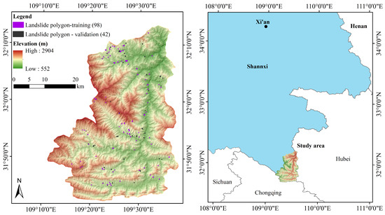
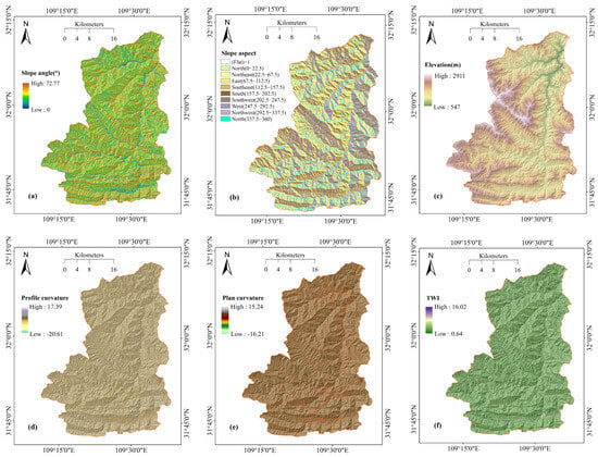
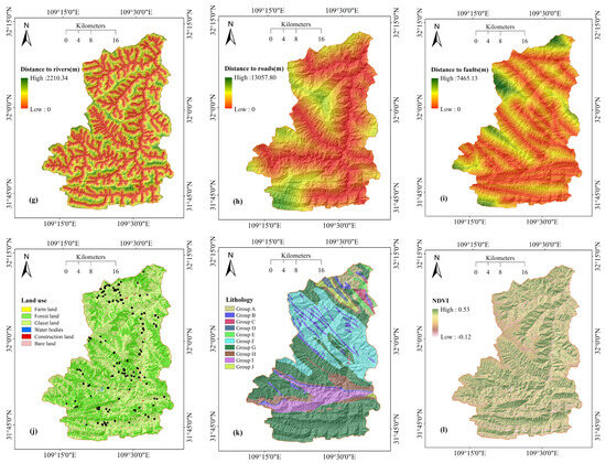
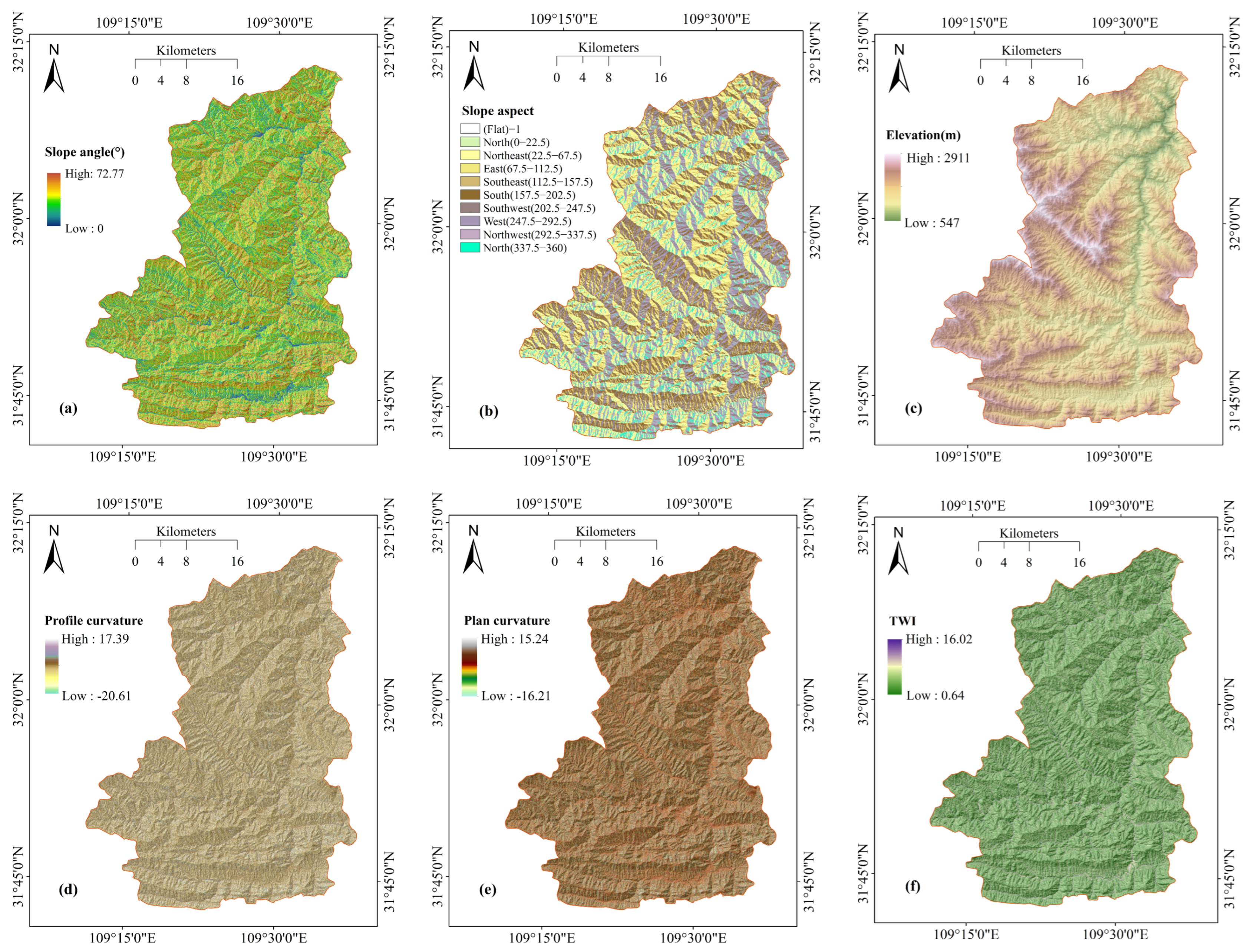
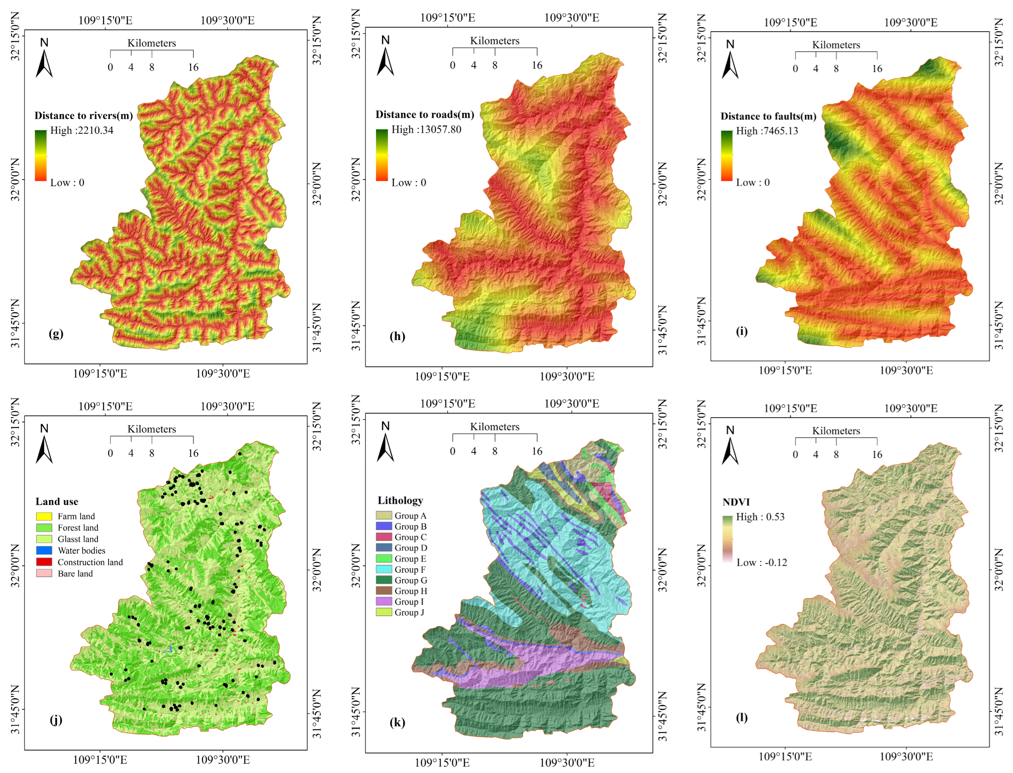
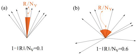
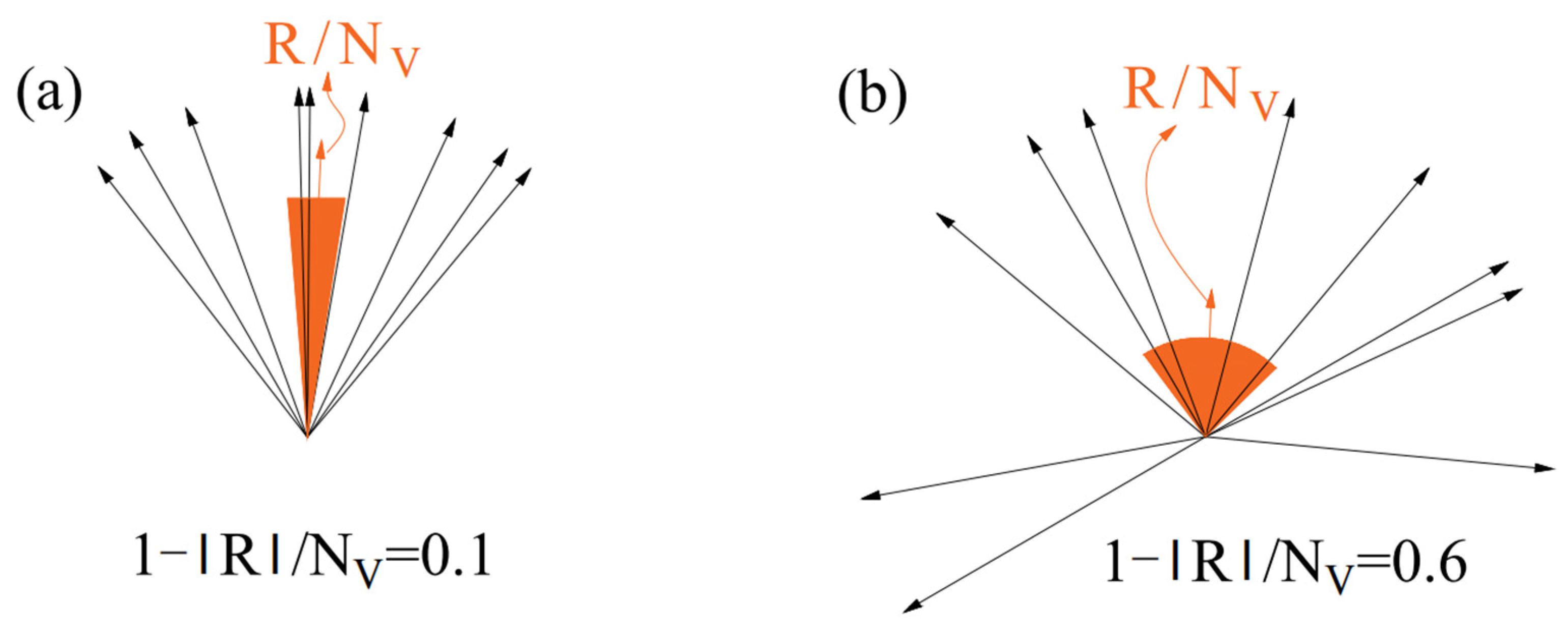
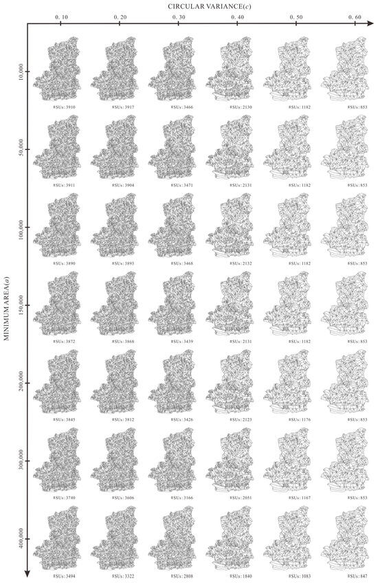
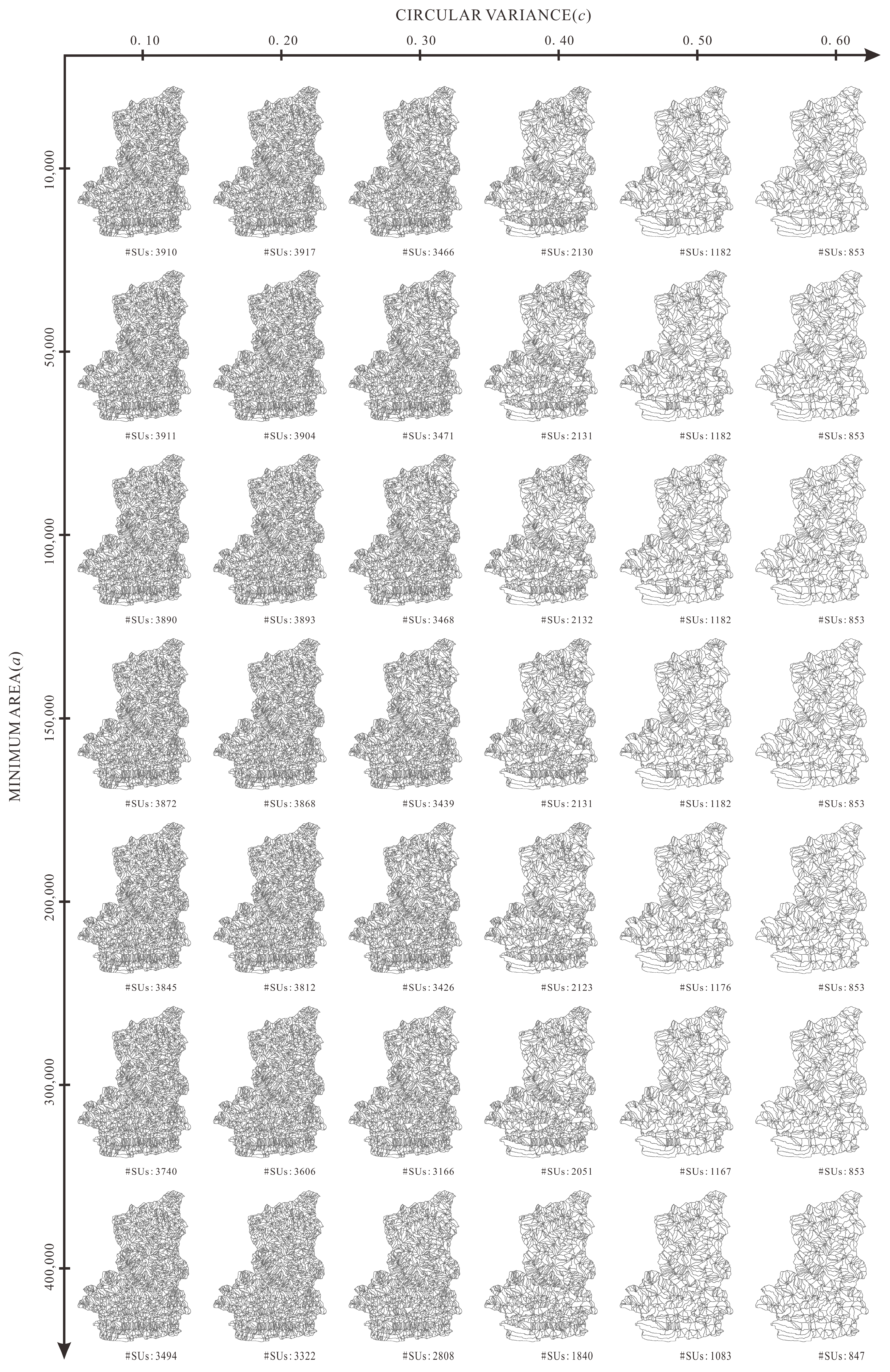
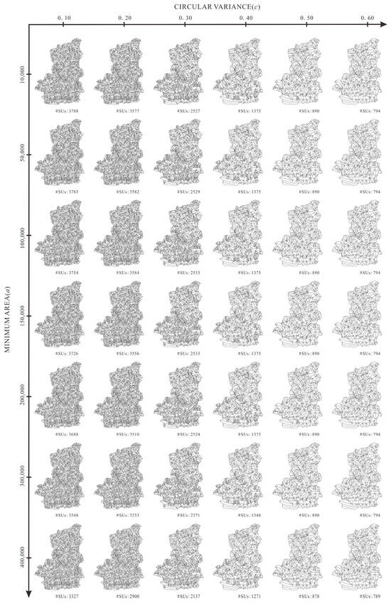
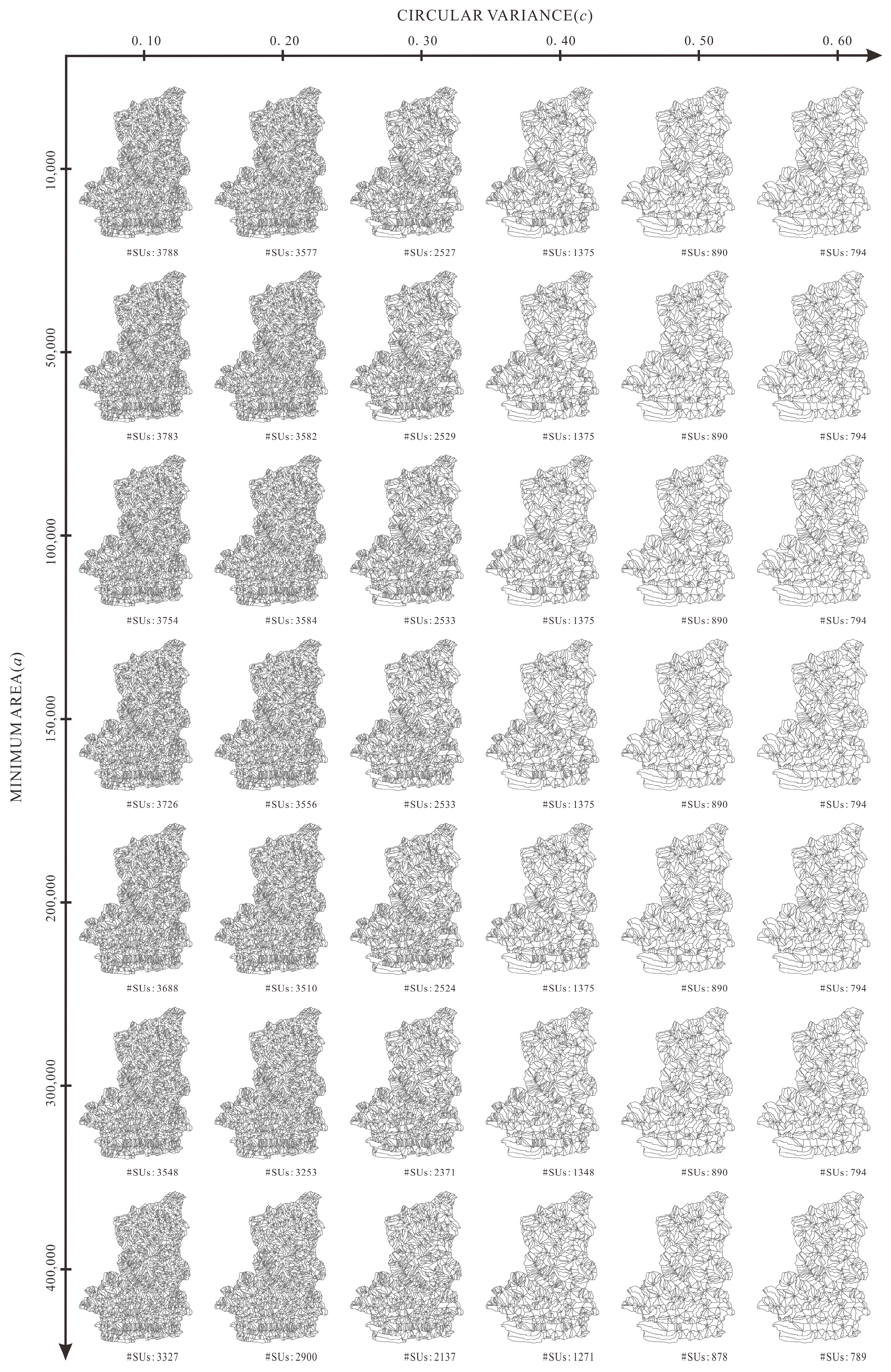
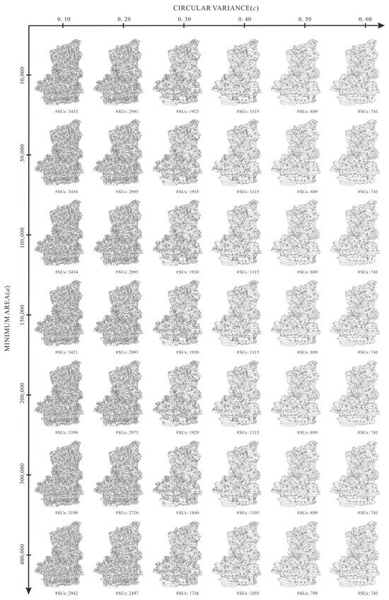
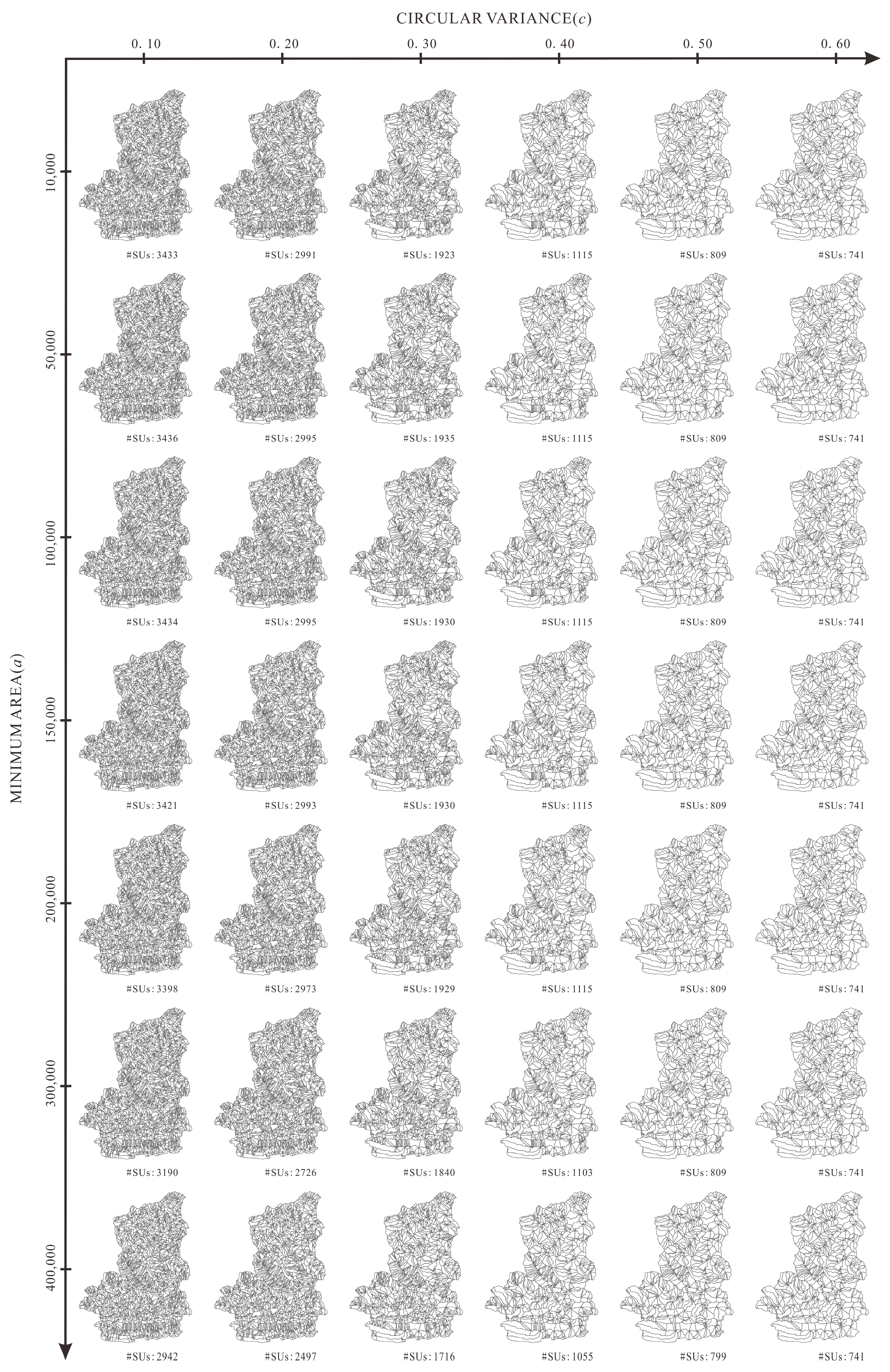
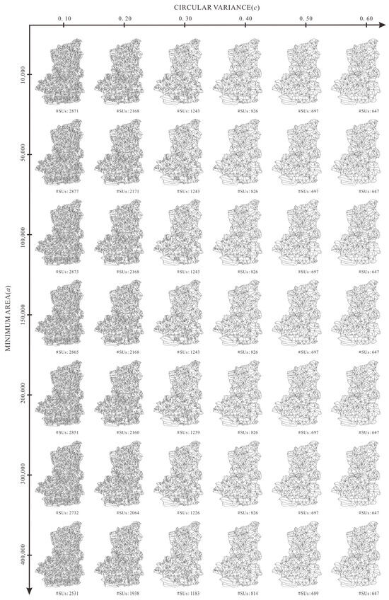
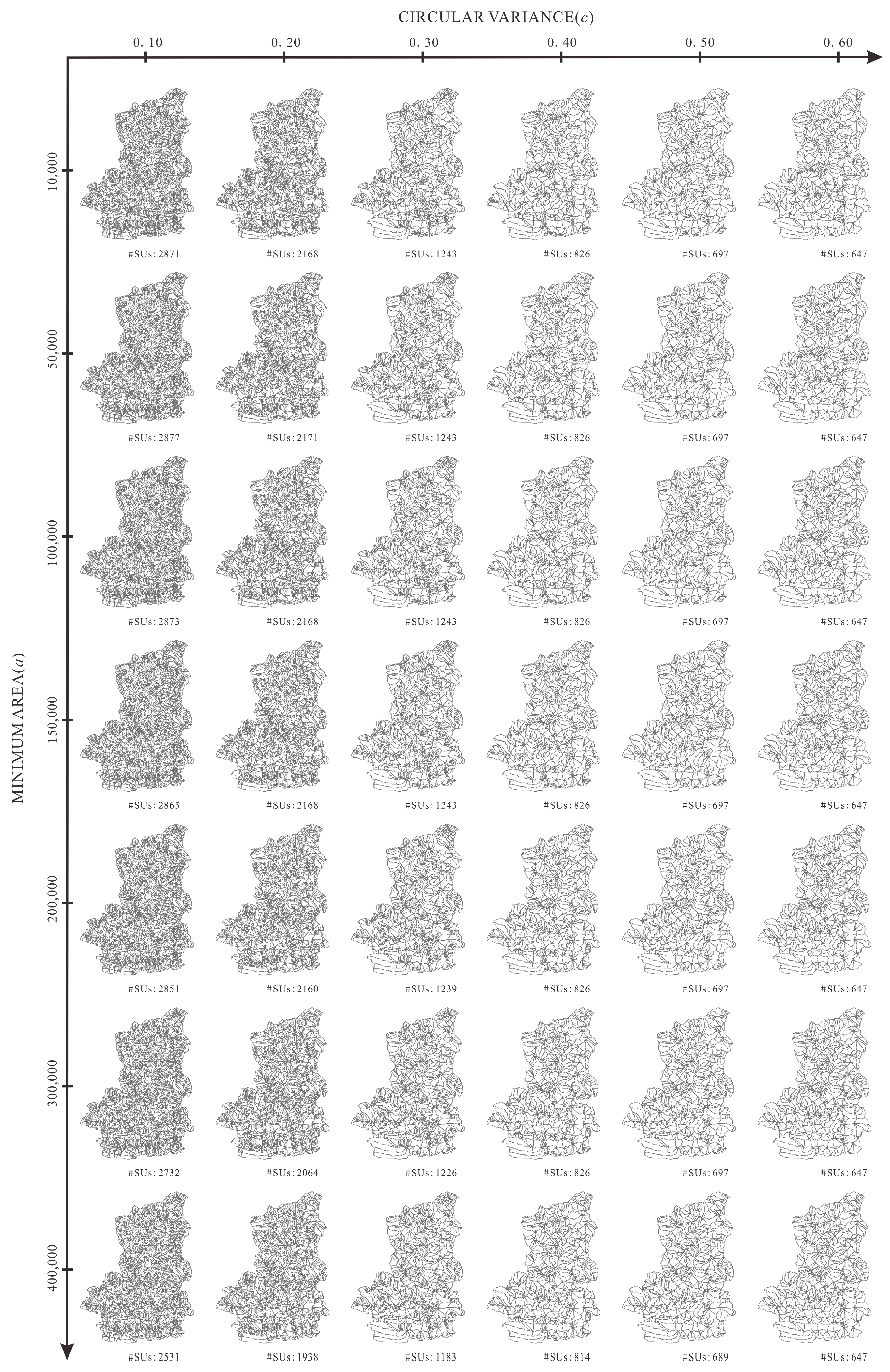
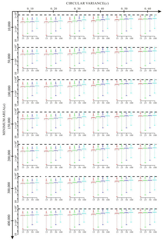
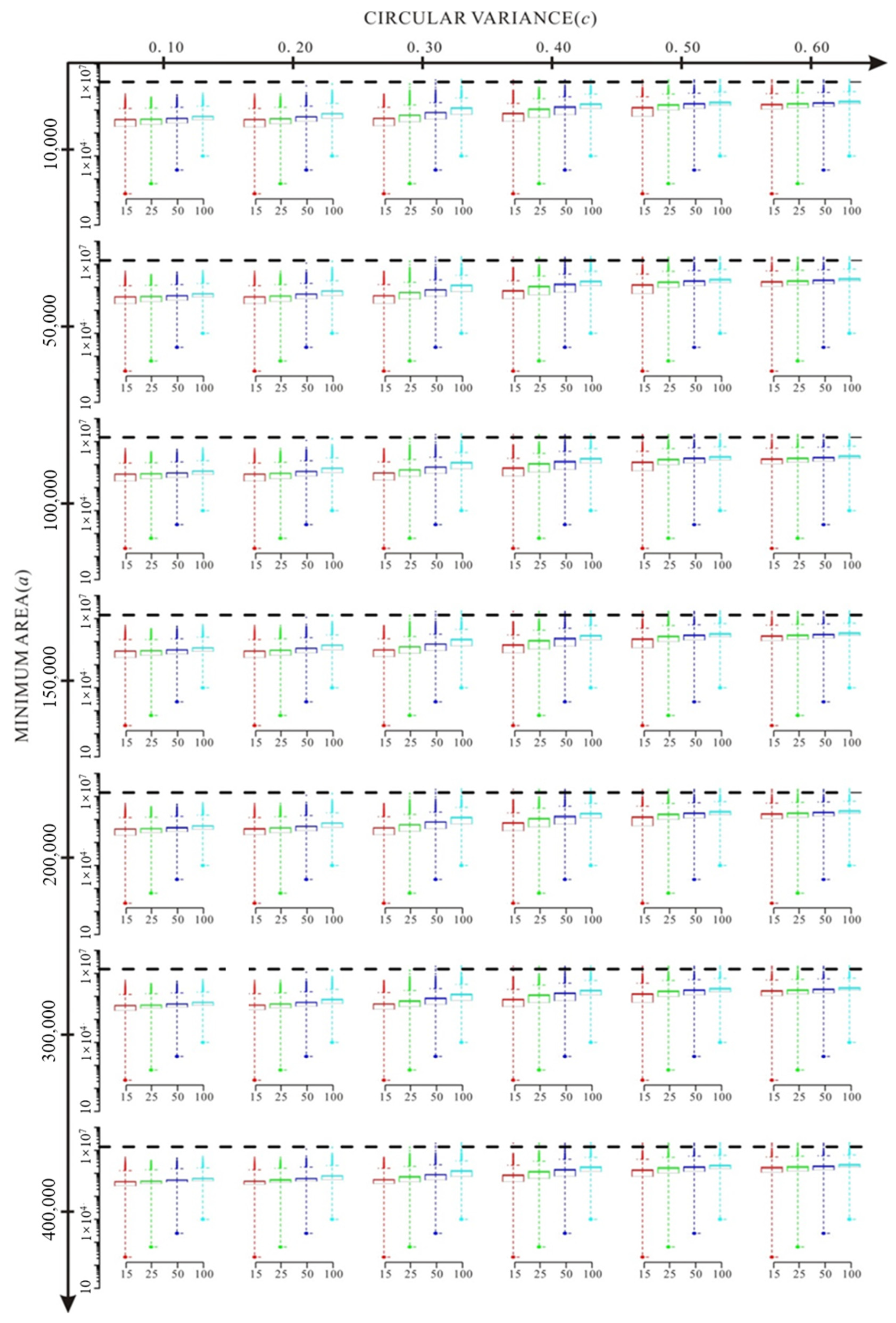
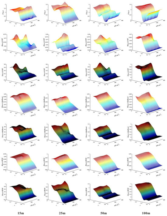
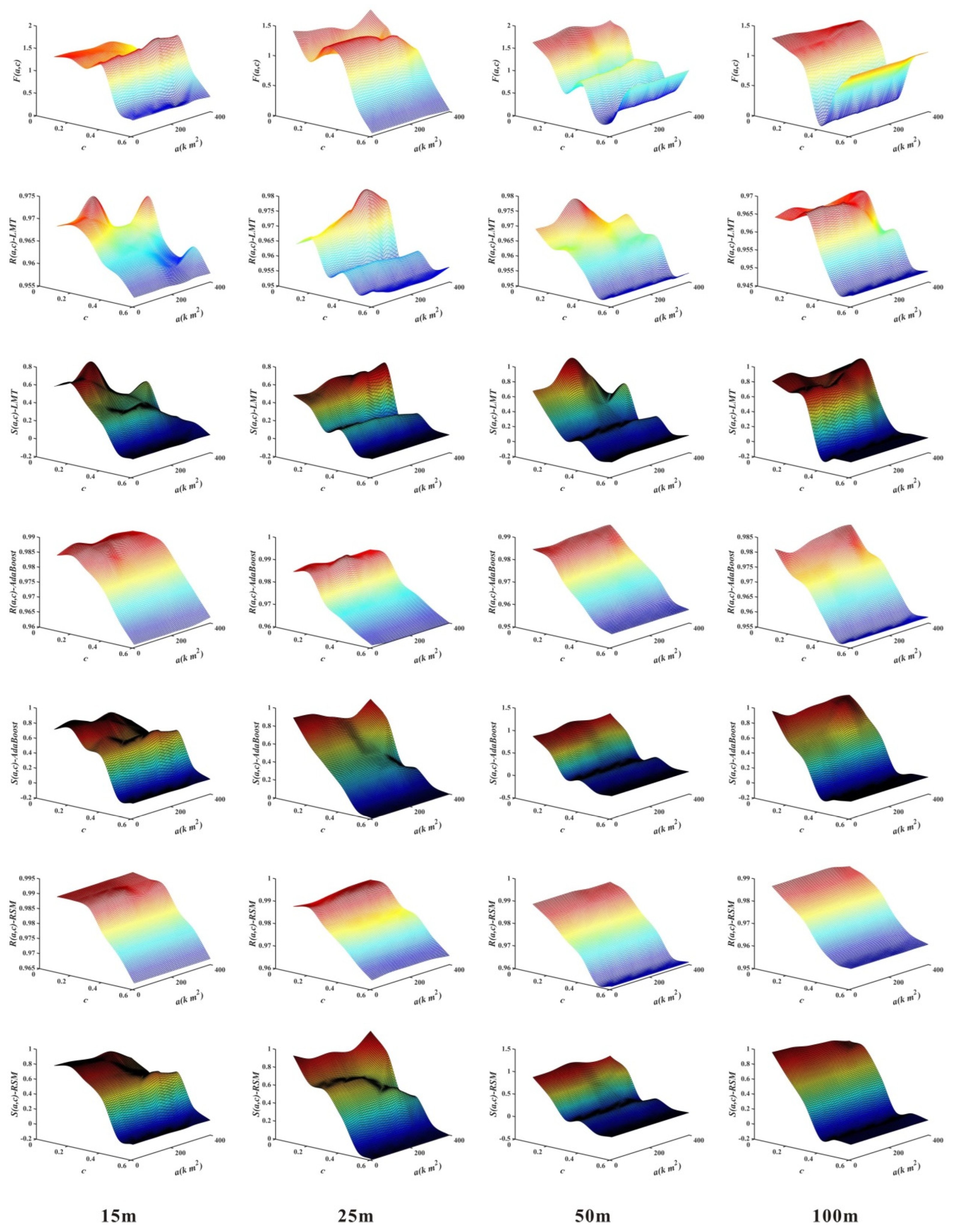
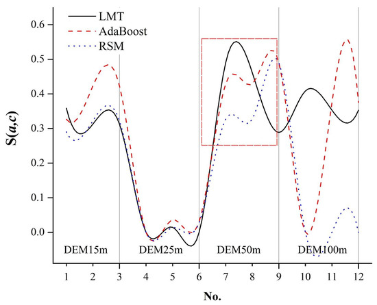
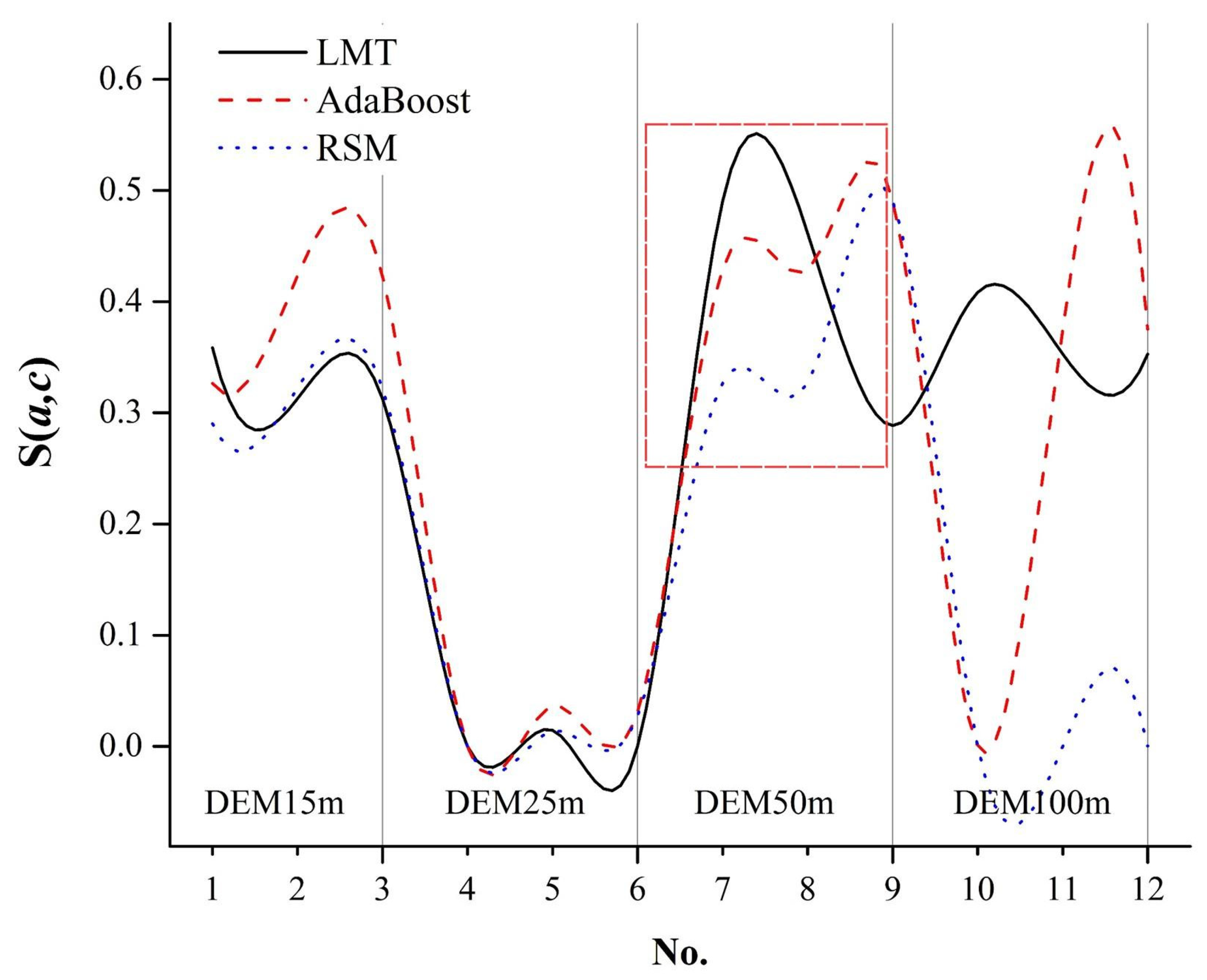
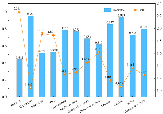
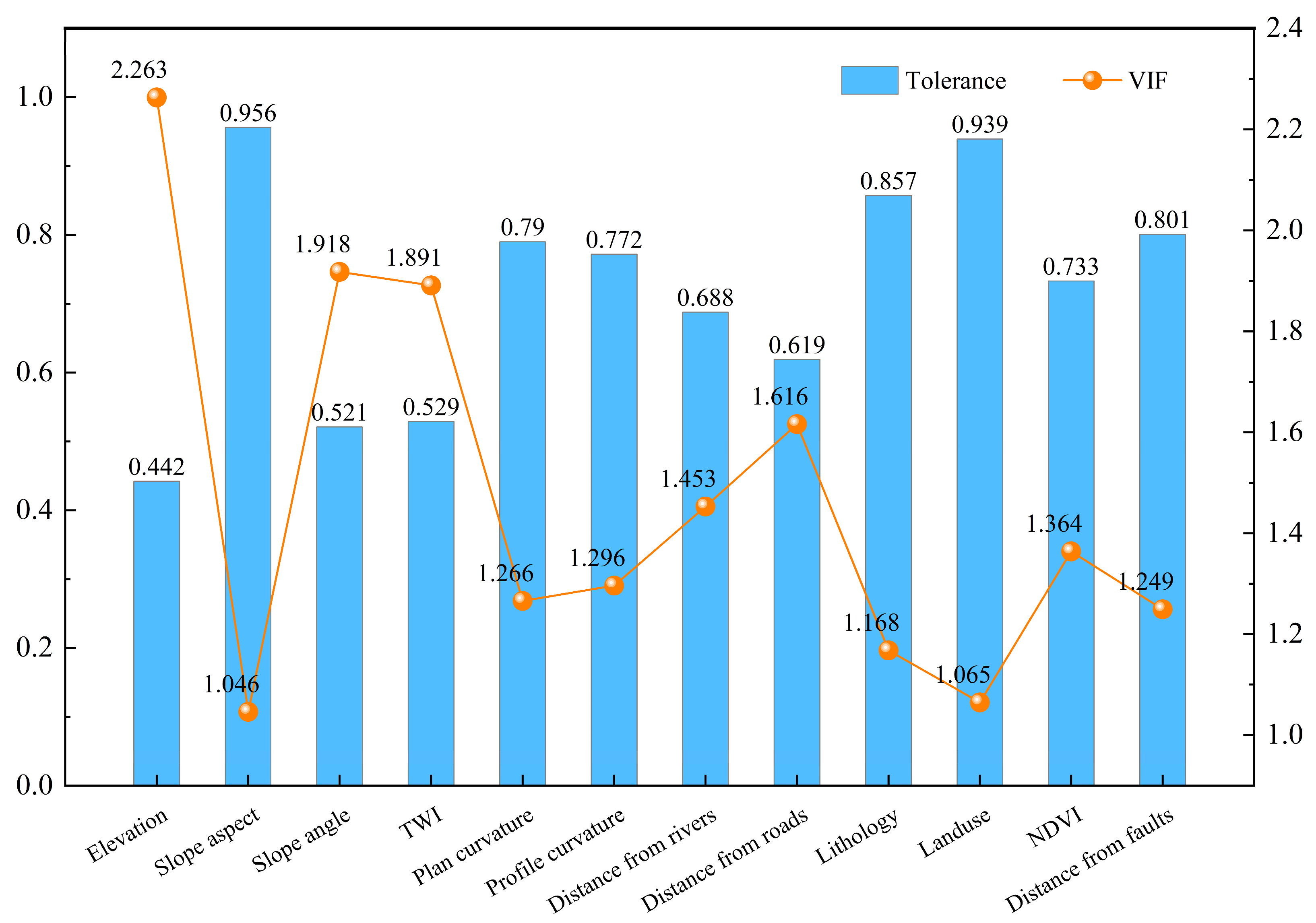
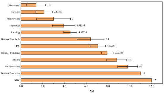
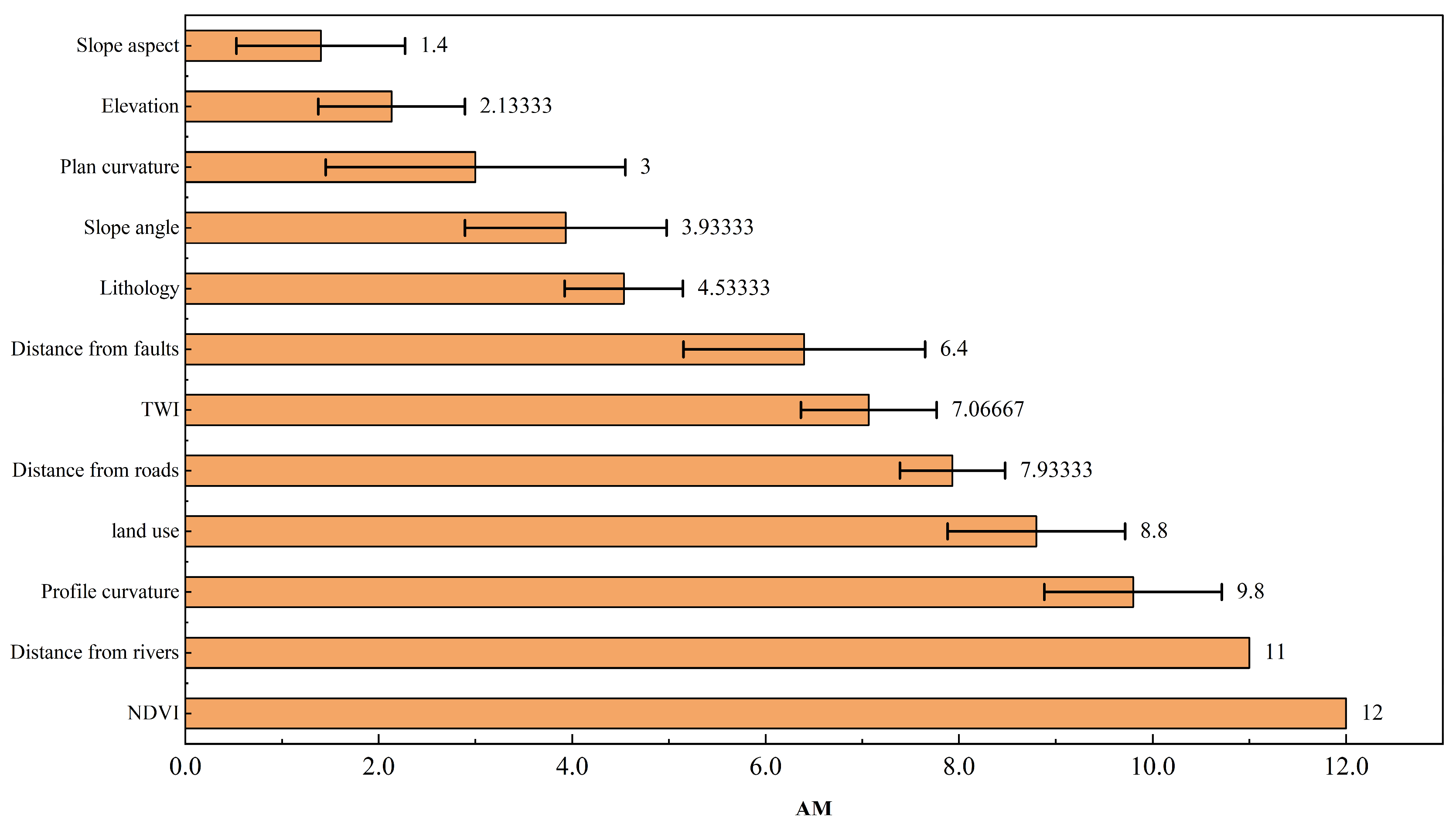
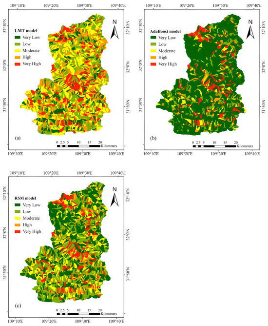
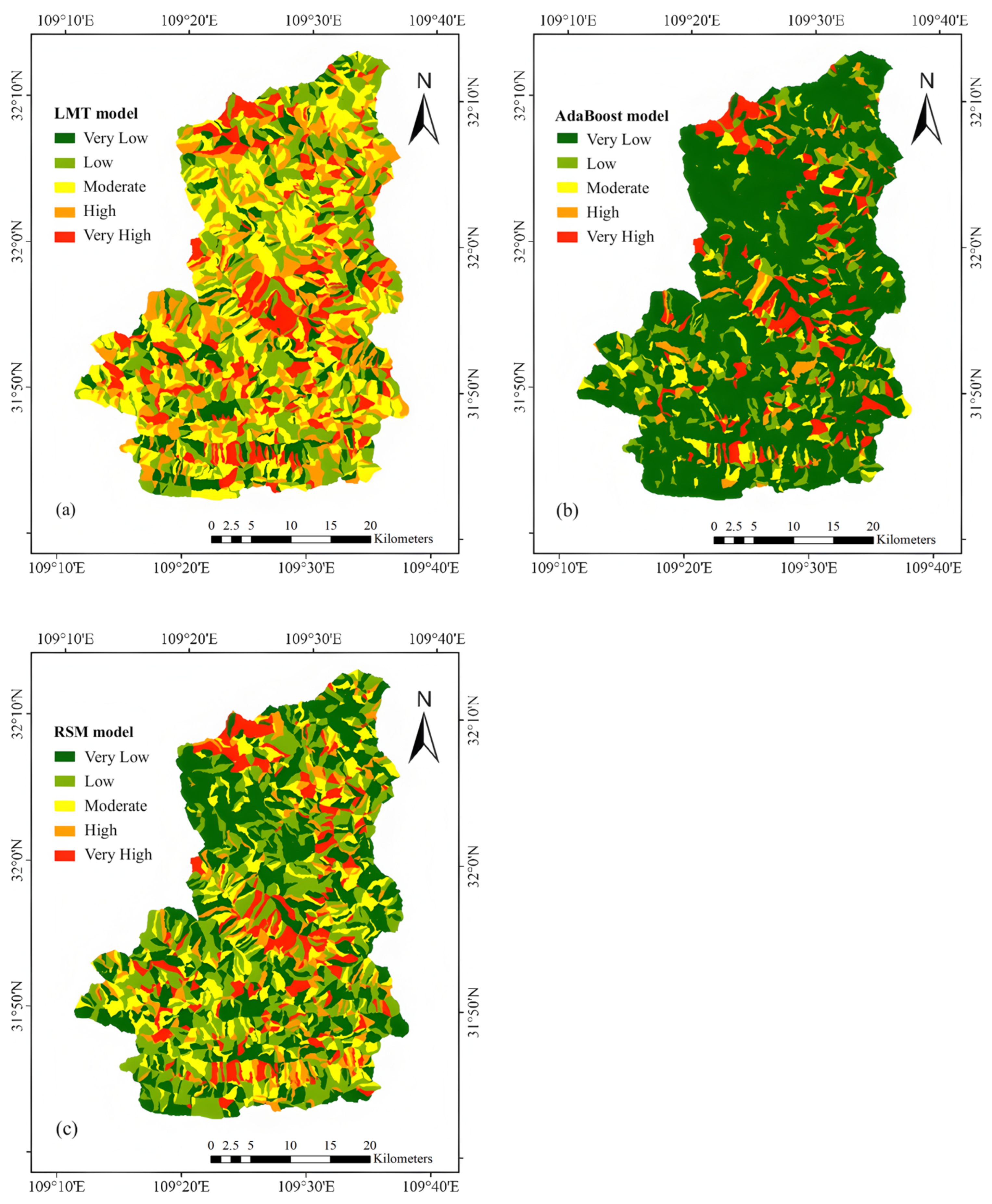
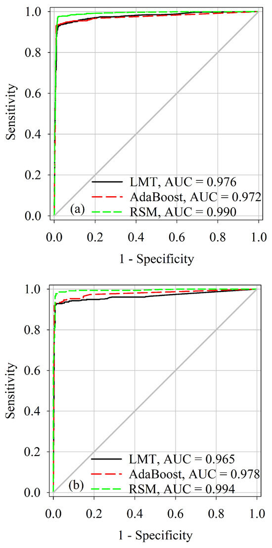
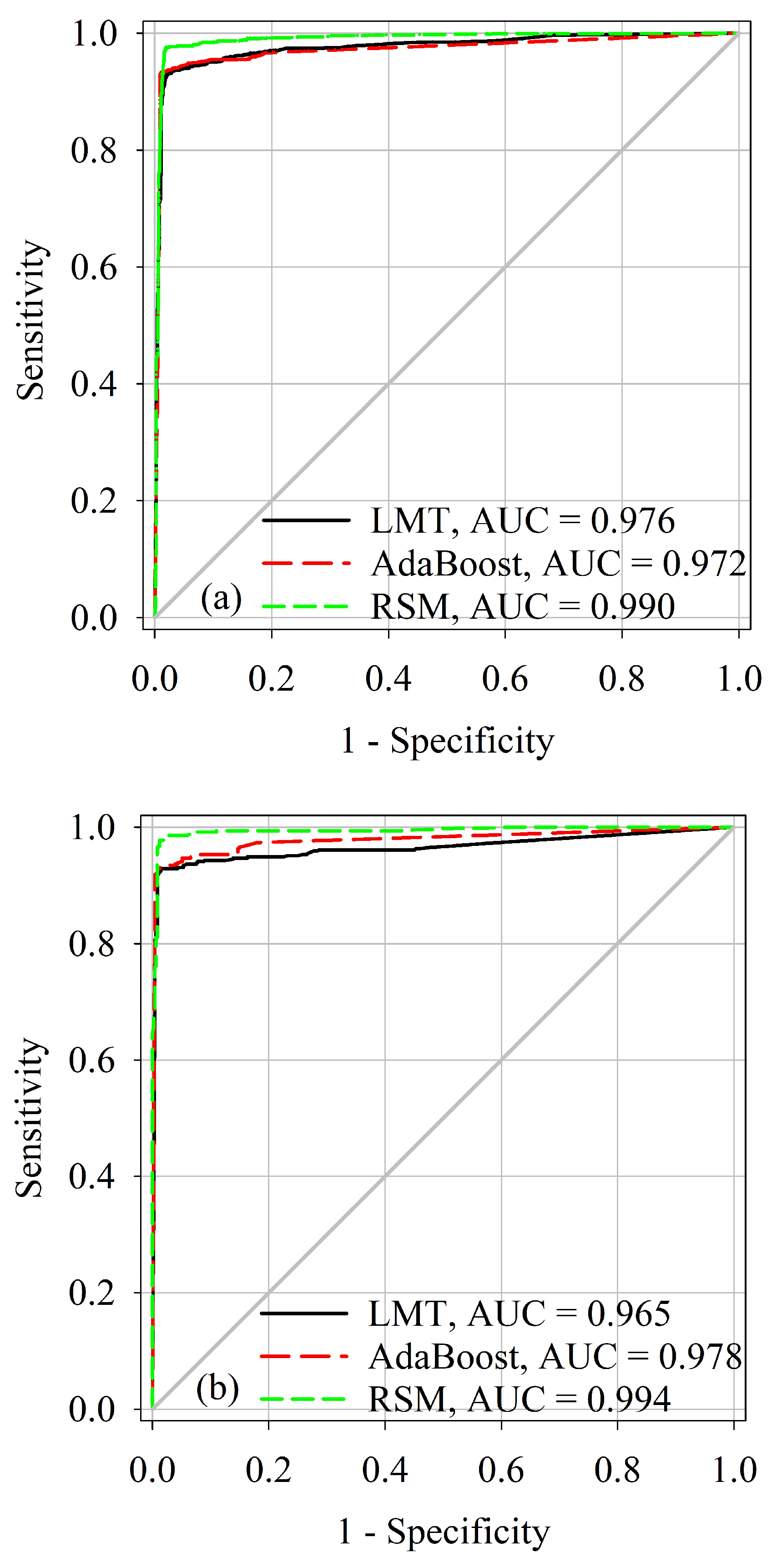

Disclaimer/Publisher’s Note: The statements, opinions and data contained in all publications are solely those of the individual author(s) and contributor(s) and not of MDPI and/or the editor(s). MDPI and/or the editor(s) disclaim responsibility for any injury to people or property resulting from any ideas, methods, instructions or products referred to in the content. |
© 2026 by the authors. Licensee MDPI, Basel, Switzerland. This article is an open access article distributed under the terms and conditions of the Creative Commons Attribution (CC BY) license.