


Highlights
What are the main findings?
- A Knowledge-Guided Factor Graph Neural Network (KG-FGNN) is proposed for online detection of attitude and orbit maneuver events of non-cooperative space targets in cross-scale, space-based optical observation scenarios.
- KG-FGNN converts domain knowledge into a computable heterogeneous graph to resolve multi-cause coupling, dynamically weights features by observation scale to emphasize reliable information, and leverages temporal residuals to exploit normal evolution predictability for isolating sudden events.
What are the implications of the main findings?
- It provides an autonomous online detection capability to support timely space situational awareness in time-critical scenarios such as rendezvous.
- The proposed framework deeply integrates knowledge guidance and data-driven learning, improving both detection accuracy and physical interpretability, and can inform other sequence analysis tasks involving complex physical coupling.
Abstract
Online abnormal event detection of non-cooperative space targets based on space-based optical observations is an urgent requirement for ensuring space security, particularly for sudden state changes such as attitude and orbit maneuver events. However, existing methods are dominated by ground-based monitoring and offline analysis, while space-based online methods are still under development and struggle to handle tasks under changing observation scales. To address this issue, we propose a Knowledge-Guided Factor Graph Neural Network (KG-FGNN). A heterogeneous graph is constructed to model high-order relationships among target properties, behaviors, observation conditions, and image features. Then, a dual-confidence dynamic weighting mechanism is designed to adaptively adjust the confidence of nodes and edges according to the observation scale. Finally, bidirectional temporal residuals are introduced to explicitly decouple sudden events from normal evolution using forward and backward prediction errors in an image sequence. Experimental results on simulated datasets demonstrate that KG-FGNN achieves higher detection accuracy for events compared to existing methods, while maintaining stable performance under cross-scale observation scenarios. This study provides an effective technical approach for online event detection in space-based optical image sequences and contributes to enhancing space situational awareness.
1. Introduction
To ensure the safety of space assets, online detection of sudden abnormal events is required when observing non-cooperative space targets from space-based platforms. Optical detection offers advantages such as long range, rich information content, and independence from target cooperation, making it a powerful technical approach for non-cooperative space target observation. However, existing methods are dominated by ground-based monitoring [1,2,3,4,5] and offline analysis [1,2,3,6], while space-based online methods [7,8,9,10] are still under development and insufficient to meet the timely perception requirements for sudden abnormal behaviors of non-cooperative targets in dynamic scenarios such as orbital rendezvous.
The majority of space targets in orbit are artificial satellites, and their behaviors can be classified into normal and abnormal. Normal behaviors are typically necessary operations for orbit maintenance or mission execution, such as smooth attitude maneuvers (change in spin angular acceleration °/s2 [11,12]) and small orbital maneuvers (change in velocity m/s [13,14,15]). If a target suddenly undergoes a large-amplitude maneuver that significantly exceeds the normal range, it is considered abnormal. For example, the target exhibits a sudden step change from three-axis stabilization to rapid rotation with spin angular velocity jumping from zero to above 5°/s, or a sudden large orbital maneuver with a velocity increment above 50 m/s. Such abnormal behaviors are the sudden events that require focused attention.
Achieving accurate event detection faces two key challenges. The first is the decoupling challenge under multivariate coupling. The observed features result from the combined effects of the target’s own behavior and the observation conditions, making it difficult to identify the true state changes caused by sudden events. The second is the lack of scale adaptability in methods. Most existing methods are designed for a single observation scale, so when the detection distance changes, they experience severe feature drift and lack cross-scale processing capability.
To address these challenges, we propose a Knowledge-Guided Factor Graph Neural Network (KG-FGNN) for event detection of non-cooperative space targets. KG-FGNN not only uses domain knowledge as a soft constraint but also embeds physical principles directly into the model’s computational structure. It uses structured prior knowledge as guidance, employs dynamic weighting to enhance multi-scale adaptability, and integrates a temporal residual decoupling mechanism to achieve accurate detection of sudden events. The main contributions are as follows:
- A heterogeneous graph is constructed to model multivariate high-order correlations among cause nodes (target properties, motion states, observation conditions) and feature nodes (image features). The graph encodes cause–feature relationships derived from optical imaging physics, converting scattered domain knowledge into a physically constrained computational prior. This computable structured topology guides the model to attribute feature variations to their underlying physical causes.
- A factor graph dynamic weighting mechanism based on dual confidence is designed. According to the observation scale, the reliability of features and the influence of causes on features are dynamically quantified as node and edge confidences. These confidences are computed as learnable monotonic functions of the target’s short-side pixel count, enabling the factor graph to smoothly recalibrate feature importance during message passing, achieving cross-scale robustness at the architectural level.
- A decoupling mechanism of a Factor Graph Neural Network (FGNN) incorporating temporal residuals is proposed. The FGNN is extended with temporal modeling via cross-frame factor reconstruction, then further equipped with bidirectional temporal residuals to strip away normal evolution patterns and explicitly decouple sudden events from observation conditions, thereby improving both detection accuracy and physical interpretability.
2. Related Work
This section first reviews existing methods for space target event detection and their limitations, then traces the development of the FGNN.
2.1. Space Target Event Detection
Existing space target event detection methods are undergoing an evolution from offline analysis to online perception and from ground-based to space-based observations.
Methods based on Two-Line Element (TLE) data accumulated by ground-based optical and radar monitoring networks [1,3] have become relatively mature. They can detect events by analyzing changes in orbital elements but are limited by data update delays and lack online detection capability. Then, researchers proposed real-time maneuver detection methods using data from ground-based monitoring networks [4,5]. Nevertheless, they rely heavily on ground-based observation systems and cannot be deployed on space-based platforms.
Subsequently, space-based optical methods have emerged, including maneuvering parameter inversion using short-arc historical data [6], approach perception using angle-only information [7], orbital maneuver detection using Line-of-Sight (LOS) measurements [8], and anomaly detection methods based on light curves [9,10]. However, these methods still have limitations in timeliness and scene adaptability: the short-arc method remains offline analysis; the angle-only method is only applicable to trend-based approaches and cannot handle sudden anomalies; the LOS method supports online processing but cannot detect attitude anomalies; the light curve methods require long-term observation accumulation and cannot adapt to fast rendezvous scenarios.
In addition, methods based on inverse synthetic aperture radar [16,17] and event cameras [18,19] have shown potential, but the technologies themselves are still immature.
In summary, existing methods still have a clear gap in online detection of sudden abnormal events of non-cooperative space targets on space-based platforms. There is an urgent need to develop a space-based optical event detection method that adapts to dynamically changing scales and can identify multiple types of sudden events.
2.2. Factor Graph Neural Network
A factor graph [20] is a probabilistic graphical model that captures local dependencies among variables by factorizing a multivariate function. Given a set of variables , if their joint distribution can be factorized into a product of factor functions, i.e.,
where . Then a bipartite graph representing the connections between variable nodes and factor nodes can be constructed, which is called a factor graph. The belief propagation algorithm on factor graphs, which iteratively passes messages to compute marginal distributions and maximum a posteriori estimates, is a classic tool for statistical inference.
Traditional factor graph methods rely on accurate model assumptions and face performance bottlenecks in high-dimensional, nonlinear, and incomplete scenarios. To overcome this limitation, Shlezinger et al. proposed learned factor graphs [20,21], where some factor nodes are parameterized as learnable neural network modules, and successfully applied them in biomedical fields [22,23,24]. Building on this, Zhang et al. further proposed FGNN [25], which fully maps the message passing and aggregation process of factor graphs into learnable layers of neural networks, enabling end-to-end learning of complex factor functions and inference rules. FGNN has already demonstrated effectiveness in structured inference tasks such as communication channel decoding [26].
The above studies have demonstrated the potential of FGNN in inverse problems. However, current research mainly focuses on static inference problems, while their application to dynamic, multivariate coupled tasks such as event detection of non-cooperative space targets is still in its infancy, representing a promising and urgently needed direction for further exploration.
3. Methods Section
This section first provides a formal formulation of space target event detection, followed by a detailed elaboration of the multivariate association heterogeneous graph, the dynamically weighted temporal factor graph, the structure of KG-FGNN, and the design of the loss function. The overall architecture of KG-FGNN is shown in Figure 1.
Figure 1.
Schematic of the KG-FGNN architecture.
3.1. Problem Formulation
The task of space target event detection aims to perform online detection of abnormal events from continuously acquired temporal image sequences and to identify the specific types of events.
Suppose the image acquired at the current time step is . It is combined with the previous multiple frames to form an image sequence of length :
A feature extractor is designed to extract features from each image:
and the feature sequence is formed as
Define the set of event labels as , where 0 denotes no event, and denote different types of events. In this study, , corresponding to attitude maneuver start/stop and orbital acceleration/deceleration, respectively. The task of event detection is to construct a multi-label detection model that takes the feature sequence as input and outputs predicted labels:
Each predicted label is a binary variable of 0 or 1. If all outputs are 0, it indicates no event; if , it means that an event of type has occurred. This output mode allows multiple types of events to occur within the same time window. The model learns to decouple the latent representations of target properties, states, and observation conditions from the image features, minimizing the discrepancy between predicted labels and ground truth.
3.2. Multivariate Association Heterogeneous Graph
In existing optical detection models for space targets [27,28,29,30], the spectral radiance at a pixel with coordinates in the image of a target is the sum of the reflected light from multiple facets on the corresponding target, given by
where is the spectral wavelength, is the conversion coefficient determined by the detection system, is the area of facet , is the distance from to the detector, is the solar irradiance reflected by , and is the earthshine irradiance reflected by ; is the solar spectral irradiance, is the solar incidence angle on , is the spectral bidirectional reflectance distribution function (sBRDF) [31] of the material corresponding to , and is the angle between the viewing direction and the specular reflection direction of sunlight on .
From (6) to (7), the causes that influence single-frame image features mainly include detection system parameters, detection distance, observation direction, illumination conditions (sunlight direction and earthshine), as well as target properties (structure, components, and material distribution) and attitude. The target properties, attitude, and observation direction determine the area, contour, and material distribution of the target’s projection onto the image plane. The detection distance, projected area, and illumination conditions affect the pixel count occupied by the target. The illumination conditions and the projected contour influence shape features. The detection system parameters, illumination conditions, and projected material distribution affect gray-level statistics, while the latter two also influence texture and spectral features.
Among the above causes, detection distance, observation direction, illumination conditions, and attitude vary over time. Detection distance is determined by the approach velocity; observation direction and illumination conditions are determined by orbital elements; and attitude is determined by the spin state. Approach velocity, orbital elements, and spin state are all time-varying causes, and thus directly affect the temporal features of the target.
Next, to clearly represent the complex influence relationships between causes and features, a heterogeneous graph [32,33] is constructed. It captures the multivariate associations and high-order couplings among multiple causes, denoted as , where and are the sets of cause nodes and feature nodes, respectively, and is the set of directed edges representing unidirectional influence relationships. The cause nodes are further divided into three categories according to their nature: property nodes , behavior nodes , and condition nodes , which describe the target’s intrinsic properties, motion state, and observation conditions, respectively.
The specific content of each node type is listed in Table 1, and the overall structure of the heterogeneous graph is shown in Figure 2 (for clarity, only some representative edges are shown). It is worth noting that directed edges exist between cause nodes, while no edges exist between feature nodes; only directed edges from cause nodes to feature nodes are present. Through this collaborative representation of multiple types of nodes, the heterogeneous graph provides more physically grounded structural prior for subsequent factor graph inference.
Table 1.
Node types in the multivariate heterogeneous graph.
Figure 2.
Overall structure of the heterogeneous graph (only representative edges are shown for clarity).
3.3. Dynamically Weighted Temporal Factor Graph
Guided by the associations in the heterogeneous graph, a temporal factor graph for space targets is constructed, and its scale adaptability is enhanced by a dynamic weighting mechanism.
First, according to the unidirectional influence relationships of target properties, behaviors, and observation conditions on image features, the cause nodes at the current time step are taken as variable nodes, and the feature nodes at the same time step are taken as factor nodes. Since a factor graph is a bipartite graph where no edges are allowed between variable nodes, all variable nodes on the same causal path are connected directly to the corresponding factor node, eliminating edges between variable nodes and implicitly encoding multi-level influence relationships into the factor function. For example, given a multi-level association , a direct edge is established, and the original edge is removed.
Next, a temporal evolution process is introduced. The factor node from the previous time step is treated as a variable node at the current time step, and the same type of factor nodes at adjacent time steps are connected to represent the evolution of target features.
The resulting temporal factor graph is denoted as , where is the set of variable nodes, is the set of factor nodes, and is the edge set. is the set of edges between and after reconnection, and is the set of edges between and across adjacent time steps.
According to the physical principles of optical imaging, under the same observation scale, the reliability of different features varies, and the reliability of the associations between features and causes also differs (i.e., the degree of influence varies). When the observation scale changes, these reliabilities change dynamically; for example, when the number of pixels on the short side of the target in the image decreases, the reliability of texture features drops. Therefore, a dynamic weighting mechanism [34,35,36,37] is introduced into the temporal factor graph. We define node confidence and edge confidence, where dynamic node confidence is defined only for factor nodes ; dynamic edge confidence describes the degree of influence of causes on features and only acts on ; the confidence of other nodes and edges is fixed to 1. The dynamically weighted temporal factor graph is illustrated in Figure 3.
Figure 3.
Dynamically weighted temporal factor graph based on target observation scale (short-side pixel count). The circles represent different nodes, and the red frame indicates the short side of the target in the images.
The dynamic node confidence is calculated based on the short-side pixel count of the target at the current time step, using a monotonically increasing Sigmoid function:
where and denote the pixel count thresholds at which feature starts to become reliable and reaches saturation, respectively. To ensure , a reparameterization is applied:
where and are learnable parameters, and the Softplus function ensures that is always positive and smooth.
Similarly, the dynamic edge confidence is expressed as
where and denote the pixel count thresholds at which the influence of cause on feature starts to become significant and reaches saturation, respectively, and and are learnable parameters.
3.4. Knowledge-Guided Factor Graph Neural Network
Based on the dynamically weighted temporal factor graph, this section further completes the construction of KG-FGNN. As illustrated in Figure 1, the network first encodes the image sequence into node embeddings, adaptively weights confidences by observation scale, and uses FGNN for cyclic feature-cause decomposition, followed by bidirectional temporal residual computation for event detection.
To better illustrate the design evolution of KG-FGNN, Figure 4 presents a step-by-step comparison from standard FGNN to the proposed framework. The standard FGNN (Figure 4①) performs bidirectional message passing between variable and factor nodes, which serves as the backbone inherited from conventional FGNN. Building upon this, the Temporal FGNN (Figure 4②) introduces temporal modeling by reconstructing current factor nodes from previous states and incorporates a reconstruction loss to preserve information, together with node/edge confidence weighting for scale adaptability. Then, the Temporal Residual FGNN (Figure 4③) further equips the network with bidirectional Gated Recurrent Unit (GRU) predictors and temporal residual computation. These extensions are not isolated additions but operate synergistically within a unified factor graph inference framework to achieve accurate detection of sudden events.
Figure 4.
Architecture evolution from standard FGNN to the proposed KG-FGNN.
3.4.1. Feature Extraction and Factor Graph Initialization
First, image features are divided into analytical and deep features. The former (e.g., pixel count, aspect ratio) have clear physical meanings and can be obtained by analytical formulas; their count is denoted as . The latter (e.g., contours, textures) represent spatial distribution patterns in images and are highly complex, and thus more suitable for learning via deep neural networks; their count is denoted as . Hence, the number of factor nodes in the factor graph is .
An analytical feature calculator containing multiple feature computation methods is designed to extract analytical features from the image:
where is a vector of length . Each component of is then broadcast to a vector of length and assigned as the factor node embedding in .
A deep feature encoder composed of a Fully Convolutional Network (FCN) and Spatial Pyramid Pooling (SPP) [38,39] then encodes the image into deep features :
where has dimensions , with the first dimension being the number of channels and the latter two spatial dimensions. Adaptive Average Pooling (AAP) is applied to adjust the spatial size of to , where (assuming is a perfect square). Then the spatial dimensions are flattened:
yielding vectors of length , which are also assigned as node embeddings to the corresponding factor nodes.
For the variable nodes in the factor graph, those belonging to are initialized with random embeddings; if some causes are known in advance, they can be linearly encoded and assigned to the corresponding nodes; those belonging to directly inherit the feature vectors from the previous time step as their node embeddings.
Next, the thresholds required by the dynamic weighting mechanism are learned from the global information in . A Global Average Pooling (GAP) is applied to , followed by a Multi-Layer Perceptron (MLP):
where , . Then, using (8)–(15), the dynamic node/edge confidences and are computed and assigned to and the edges in . The confidences of , and edges in are fixed to 1.
At this stage, all nodes have obtained their initial embeddings and confidences, and all edges have also obtained their corresponding confidences. The factor node embeddings are denoted as , the variable node embeddings belonging to as , and the variable node embeddings belonging to as .
3.4.2. Factor Graph Neural Network with Temporal Residuals
For the image sequence within a detection window, the above steps yield temporal factor graphs, denoted as . Among them, has no previous image, so it does not contain the corresponding , , or .
FGNN is used to compute variable node embeddings frame by frame. To adapt to the temporal characteristics of space-based observations, the original FGNN is specifically modified. The FGNN is divided into a Factor-to-Variable (F2V) module and a Variable-to-Factor (V2F) module. The former is still used to decompose features into causes, while the latter is changed to reconstruct the current features from the causes and the previous-time-step features, expressed as
where is an aggregator, and and are the MLP layers of the F2V and V2F modules. A message passing mechanism with a fixed number of iterations is adopted. In each iteration, (20) updates the variable node embeddings of to ; known assigned variable nodes can be unchanged. The factor node embeddings and the variable node embeddings of are not updated. After iterations, (21) reconstructs , which is then used to compute the feature reconstruction loss.
At this point, the updated variable node embeddings and the reconstructed factor node embeddings are obtained (feature reconstruction is not performed for because it lacks ).
Next, to enhance sensitivity to sudden events, a bidirectional temporal residual mechanism is introduced. For consecutive frames in the middle of the time window (), the start index and end index are defined as
where is the floor operation.
As illustrated in Figure 5, for each intermediate frame , the node embeddings of the current frame are predicted using both historical frames (forward) and future frames (backward) within the window, and bidirectional residuals are computed. It should be noted that to ensure real-time performance, the detection delay must be less than the task tolerance, i.e.,
where is the image acquisition frame rate, is the average detection delay, and is the maximum tolerable delay for the task.
Figure 5.
Schematic of the bidirectional temporal residual computation process.
Specifically, the forward GRU is first used to predict the intermediate frame’s from its historical frames:
where denotes the forward predictor. Then, together with are fed into (21) to reconstruct and the forward residual is computed:
Similarly, the backward GRU is used to predict the current frame from its future frames, yielding the backward residual :
where denotes the backward predictor.
Finally, all forward and backward residuals of the intermediate frames are concatenated and fed into a Multi-Head Multi-Layer Perceptron (MHMLP) to obtain the final event detection result:
where , , is the multi-label detector, and is the predicted result for event type .
This design allows the residuals to directly reflect the deviation of actual features from the normal evolution pattern, explicitly decoupling sudden events from observation conditions.
3.5. Loss Function
The loss function of KG-FGNN consists of a dynamic weighting regularization loss, a feature reconstruction loss, a property consistency loss, and an event detection loss. Specifically, the following applies.
Dynamic weighting regularization loss is used to constrain the value ranges of , keeping the dynamic changes in node/edge confidence within reasonable bounds. It is expressed as
where , , and and can be set according to the distribution of target features in the observed images.
Feature reconstruction loss is used to constrain the accuracy of the V2F module in reconstructing image features, ensuring that the latent variables contain sufficient information. It is expressed as
where , , is the Mean Absolute Error (MAE), and the subscript indicates averaging over all corresponding terms.
Property consistency loss is used to enforce that the intrinsic properties of the target remain unchanged during temporal prediction; i.e., the property node embeddings in the variable nodes stay constant within the same time window. It is expressed as
where , .
Event detection loss is used to enforce consistency between the multi-label detection results and the ground-truth events. It is expressed as
where , is the predicted result, is the ground truth, and is the cross-entropy function, with the subscript indicating averaging over all corresponding terms.
The final loss function is a weighted sum of the above terms:
where are the weights of each loss term. The multiple losses are jointly optimized to improve the accuracy and physical interpretability of event detection.
4. Results
This section describes the experiments and results. First, the datasets are introduced, followed by a detailed explanation of the experimental setup. Finally, the experimental results are presented to validate the performance of the proposed method.
4.1. Datasets
Existing public datasets for space targets mostly consist of light curves or static high-resolution images [40,41,42,43], lacking sequential image data for event detection. Therefore, we generate high-fidelity sequential images using a Hardware-in-the-Loop (HIL) simulation method for space targets based on dynamic scenes [44] to support the research and validation of event detection methods.
4.1.1. Event Label Definition
We focus on large-amplitude sudden abnormal events, as summarized in Table 2.
Table 2.
Definition of abnormal events.
Since the normal behaviors of space targets are necessary operations to maintain attitude and orbit stability, and after successful execution the target remains in a normal operational state, they are not additionally simulated.
4.1.2. Scenario-Specific Decoupled Combination Generation Strategy
To balance data diversity and generation efficiency, we adopt a scenario-specific decoupled combination generation strategy to produce the simulation datasets, obtaining multiple image sequences under different observation scenarios. Each sequence lasts approximately 9–15 s, with a frame rate of 15 FPS and 1–3 events. Starting from the orbital coordinate system of the space-based platform, two types of key causes affecting the observational data are decoupled:
- Orbital geometry: including detection distance and LOS angles, determined by the relative motion between the space-based platform and the target, used to simulate orbital maneuver events.
- Imaging geometry: including solar phase angle and target attitude, which determine the imaging characteristics of the target, used to simulate attitude maneuver events.
Within an observation period of about ten seconds, the solar phase angle remains nearly constant in co-orbital scenarios, while it shows a continuous trend of change in rendezvous scenarios. To maintain macroscopic physical plausibility, co-orbital and rendezvous scenarios are designed separately; orbital geometry sequences and imaging geometry sequences are independently generated for each scenario and then randomly paired and combined to obtain a large number of physically self-consistent simulation sequences. The specific generation methods are as follows:
Orbital geometry sequences are generated using the orbit integration method based on the two-body dynamics model [8]. It takes the orbital elements of the space-based platform and the target as initial inputs and sets the specific time of the orbital maneuver, as well as the direction and magnitude of the velocity change. By solving the two-body motion equations through high-precision numerical integration, an instantaneous velocity pulse is applied at the preset event time to simulate the orbital maneuver, and then the integration continues to the end of the simulation, thereby obtaining sequences of detection distance, approach velocity, and LOS angles (i.e., the azimuth and elevation of the observation direction in the orbital coordinate system).
Imaging geometry sequences are generated by calculating the geometric relationship among the sun, target, and detector at multiple time instants, based on the set orbital elements, spin axis direction and spin angular velocity, as well as the occurrence time and magnitude of attitude maneuver events, yielding the solar phase angle and the relative attitude sequence of the target.
4.1.3. HIL Simulation
Then, according to the two types of cause sequences, sequential images are acquired through HIL simulation experiments.
We design an on-orbit space-based detection system and an HIL simulation detection system based on space-based observation requirements [45,46,47] and HIL conditions. Both systems are staring visible-band spectral imaging systems based on an Acousto-Optic Tunable Filter (AOTF), featuring coaxial common field-of-view (FOV) panchromatic and spectral channels. Their specifications are shown in Table 3. The systems acquire data in groups; each group takes 3 s to measure and contains 45 panchromatic/spectral image pairs, covering a wavelength range of 440 nm to 780 nm.
Table 3.
Specifications for the space-based and HIL simulation detection systems.
In the HIL experiments, the imaging geometry sequences are transformed into the coordinate system of the HIL platform, and the simulation detection system is used for image acquisition, followed by image background removal and spectral reflectance inversion. Finally, to match the resolution of the on-orbit system, the panchromatic and spectral images are downsampled according to the detection distance in the corresponding orbital geometry sequences, obtaining simulation image sequences that are consistent with on-orbit observation conditions.
It should be noted that the decoupled combination strategy uses relative quantities in the detection coordinate system instead of absolute orbital parameters. This suffices to characterize feature changes and aligns with space-based observation practice, so the validation of event detection is not affected.
We selected three satellites as targets: GAOFEN-6 in Low Earth Orbit (LEO), BEIDOU-2 M5 in Medium Earth Orbit (MEO), and BEIDOU-2 G2 in Geostationary Earth Orbit (GEO). The maximum length of GAOFEN-6 is approximately 8 m, and its main body dimensions are approximately 1.7 m × 1.8 m × 2 m. The maximum length of BEIDOU-2 G2/M5 is approximately 17.5 m, and its main body dimensions are approximately 2.2 m × 1.7 m × 2.3 m.
A 30:1 scaled model of GAOFEN-6 and a 35:1 scaled model of BEIDOU-2 were used as HIL targets. The models include typical components such as the main body, solar panels, and antennas, and are covered with six typical materials: gold mylar, solar cell, aluminum, carbon fiber, lens, and white paint. Among these, the first four materials are common to both scaled models; the lens is unique to GAOFEN-6, distributed on its Earth observation payload; and the white paint is unique to BEIDOU-2, distributed on its parabolic antennas. The two models and their material reflectance spectra are shown in Figure 6 and Figure 7.
Figure 6.
Space target scaled models. (a) GAOFEN-6 model (30:1); (b) BEIDOU-2 model (35:1).
Figure 7.
The reflectance spectra of space target model materials. (a) Reflectance spectra of materials with larger surface coverage. (b) Reflectance spectra of materials with smaller surface coverage.
During the simulation of GAOFEN-6, because it operates in LEO and is illuminated by both sunlight and earthshine, a tungsten halogen lamp was used as a solar simulator, and indoor uniform diffuse ambient light was used to simulate earthshine, with the latter being significantly dimmer than the former. For the simulation of BEIDOU-2 G2/M5, as it operates in MEO and GEO where the energy of earthshine has decayed to a negligible level, we used a darkroom environment and only a solar simulator. The schematic diagrams and photographs of the HIL simulation experiments for both cases are shown in Figure 8.
Figure 8.
Space target HIL simulation experiments. (a) Schematic of experiments for GAOFEN-6. (b) Schematic of experiments for BEIDOU-2. (c) Photograph of experiments for GAOFEN-6. (d) Photograph of experiments for BEIDOU-2.
Finally, for the three targets, three HIL simulation datasets were generated. The datasets contain 140 simulation image sequences, with a total duration of 1530 s and 22,950 panchromatic/spectral image pairs, including a total of 280 attitude/orbit maneuver events of the targets. The simulation parameter configurations for each target are listed in Table 4. The detection distance ranges from 50 to 1000 km, and the solar phase angle ranges from 30° to 130°. The relative attitude of the target is intuitively represented by the observation azimuth and observation elevation angles in the target’s body coordinate system, with the observation azimuth covering 0° to 360° and the observation elevation ranging from −3° to 53°. The change in relative spin angular velocity during attitude maneuver events ranges from 6.1 to 9.6°/s, and the change in approach velocity during orbital maneuver events ranges from 50 to 95 m/s.
Table 4.
Parameter configurations for the space target space-based detection simulation.
GAOFEN-6 and BEIDOU-2 M5 are set as co-orbital scenarios, where the detection distance and solar phase angle change very little, the approach velocity ranges from −0.1 to 0.4 km/s, and the rate of change in the solar phase angle ranges from −0.1 to 0.1°/s. BEIDOU-2 G2 adopts rendezvous scenarios, with an approach velocity ranging from −1.28 to 4.65 km/s (including both the approaching phase before rendezvous and the receding phase after rendezvous), and the change rate of the solar phase angle ranges from −9.2 to −0.2°/s. The variation trends of the parameters in each simulation sequence conform to the physical characteristics of the corresponding scenarios, providing sufficiently diverse samples for subsequent model training and evaluation.
Examples of single-frame images in the datasets are shown in Figure 9, including schematic diagrams of the target’s attitude, raw acquired images after background removal, and simulated images matched to the on-orbit system. As the detection distance increases, the spatial details in the panchromatic images gradually decrease: from resolved targets (detection distance 50–300 km, short-side pixels ≥ 20) to partially resolved targets (detection distance 300–800 km, short-side pixels 5–20), and finally to unresolved targets (detection distance 800–1000 km, short-side pixels ≤ 5), where spatial features become almost unavailable. The spatial resolution of the target in the spectral images is lower than that of the panchromatic images, and the spectral images are mainly used to provide material-related spectral information.
Figure 9.
Simulated image examples of space targets at different detection distances in the datasets. The red frames indicate the target areas in the simulated panchromatic images. The colors in the attitude illustrations correspond to different material types, as shown in Figure 7.
Examples of image sequences are shown in Figure 10 and Figure 11, illustrating the evolution of target features over time under different scenarios, as well as the changes in the relative spin angular velocity and approach velocity of the target when attitude and orbital maneuver events occur. It can be observed that the image features are affected by the coupled influences of factors such as attitude and detection distance, exhibiting complex nonlinear variation patterns. This constitutes a primary challenge in space target application missions.
Figure 10.
Image sequence example 1 (target: GAOFEN-6, scenario: co-orbit, events: attitude maneuver start/stop and orbital deceleration).
Figure 11.
Image sequence example 2 (target: BEIDOU-2 G2, scenario: rendezvous, events: attitude maneuver start and orbital deceleration).
4.2. Experimental Setup
This section describes the sample generation method, implementation details, and evaluation metrics.
4.2.1. Sample Generation
A temporal sample generation strategy combining a sliding window with soft labels was adopted [48,49,50]. Each sample consists of 10 consecutive frames, with a stride of 1 frame. A sample is labeled as positive if the frame difference between its central frame and any event frame is within 3 frames; otherwise, it is labeled as negative. The 140 sequences were divided into training, validation, and test sets in a ratio of 5:2:3. Specifically:
- After generation, the training and validation samples were randomly shuffled. The sampling ratio was adjusted to maintain an approximate 1:1:3 proportion among attitude maneuver positive samples, orbit maneuver positive samples, and event-free negative samples, thereby preventing the proposed method from biasing toward negative predictions due to class imbalance.
- The test set was generated in the original temporal order of the sequences to simulate an online detection scenario.
The event type distribution of samples across the training, validation, and test sets is shown in Table 5. It should be noted that a small number of samples contain both attitude and orbit maneuver events; therefore, the sum of the sample counts across event types slightly exceeds the total number of samples.
Table 5.
Sample statistics of different event types in training, validation, and test sets.
4.2.2. Implementation Details
The implementation, hyperparameter configuration, and training details are described below. The specific analytical features adopted in this study are listed in Table 6. The selected known causes include detection system parameters, detection distance, observation direction, and sunlight direction, all of which are observation conditions that can be acquired in real time. Their detailed contents and acquisition methods are provided in Table 7. Notably, the current accuracy of space-based ranging methods is on the order of kilometers [51,52,53,54,55], which is insufficient to serve as a direct criterion for orbit maneuver events but can be used as prior information to assist event detection.
Table 6.
Different types of analytical features and their source images.
Table 7.
Contents and acquisition methods of the known causes.
The complete implementation and configuration of the model are presented in Table 8, where the network structures and hyperparameters of feature extraction, node embedding, dynamic weighting, FGNN, temporal residual, and loss function are listed by processing phase. During training, the batch size was set to 10, and the total number of epochs was 100. The Adam optimizer was used with an initial learning rate of 0.001. An adaptive learning rate decay strategy was applied: the learning rate was multiplied by a factor of 0.1 when the validation loss failed to decrease over five consecutive epochs.
Table 8.
Details of implementation and configuration.
4.2.3. Evaluation Metrics
All samples in a sequence are fed into the model in temporal order to obtain frame-wise detection results. Different event types are processed independently. For event type , a sample is considered positive if its confidence score exceeds the corresponding threshold . Temporally consecutive positive samples are merged into predicted segments, taking the highest-confidence frame in each as its representative, yielding non-overlapping predicted segments.
For each event type, all temporally consecutive samples with positive soft labels are merged to form the ground-truth event windows. A predicted segment is regarded as a correct detection if its Temporal Intersection over Union (TIoU) [56] with the corresponding event window is no less than 0.5 and the predicted label matches the ground-truth event type; otherwise, it is considered incorrect.
Precision, recall, and F1-score are adopted as evaluation metrics and are calculated separately for each event type as follows:
where is the number of correctly detected predicted segments, is the total number of predicted segments, and is the total number of ground-truth events.
To determine the optimal threshold for each event type, we use the validation set reorganized in the original temporal order of the sequences. Multiple computations are performed over the range [0.01, 0.99] on the validation set, and the configuration yielding the highest F1-score is selected as the final result. These selected thresholds are then applied to the test set to report the performance. Finally, the overall precision, recall, and F1-score are obtained by aggregating the total number of correct detections, predicted segments, and ground-truth events across all event types.
4.3. Experimental Results
This section presents a comprehensive evaluation of the trained KG-FGNN. The overall performance is first reported, followed by comparisons with existing methods, an ablation study, model interpretability visualization, and noise adaptability evaluation.
4.3.1. Detection Performance
KG-FGNN was evaluated on the test set, and the evaluation metrics for different targets, event types, and the overall performance are shown in Table 9 and Table 10. The F1-score curves for each event type at different thresholds on the test and validation sets are shown in Figure 12.
Table 9.
Performance metrics for event detection on different targets.
Table 10.
Performance metrics for different event types.
Figure 12.
F1-score curves of event detection on the test and validation sets (the red lines indicate the best thresholds of events). (a) Attitude maneuver start; (b) attitude maneuver end; (c) orbit maneuver acceleration; (d) orbit maneuver deceleration.
It can be seen that, under the optimal threshold settings, the proposed method achieves an overall F1-score of 0.844, validating its effectiveness on the event detection task. In terms of individual targets, BEIDOU-2 M5 and BEIDOU-2 G2 show comparable performance with F1-scores of 0.850 and 0.869, respectively, whereas GAOFEN-6 reaches only 0.765, revealing a notable performance gap.
With respect to event types, attitude maneuver start and end events show comparable detection performance, both achieving an F1-score of 0.930, indicating the method’s high detection sensitivity for attitude maneuvers. In contrast, orbit maneuver events are considerably more challenging to detect. The F1-scores for orbit maneuver acceleration and deceleration are 0.800 and 0.703, representing the performance bottleneck of the method. Furthermore, the F1-score curves demonstrate that attitude maneuver events maintain relatively high and stable performance across a wide range of thresholds, whereas orbit maneuver events are noticeably more sensitive to threshold variations, further reflecting the greater difficulty in their detection.
4.3.2. Comparative Experiments
Existing methods suitable for optical space-based online event detection can be broadly divided into two categories: orbit maneuver detection methods based on LOS angle measurements and attitude maneuver detection methods based on light curve analysis. We select one recent representative method from each category as a baseline: Space-based Passive Orbital Maneuver Detection (SPOMD) [8] from 2024 for binary orbit maneuver detection and Temporal-Attention Long Short-Term Memory network (TA-LSTM) [10] from 2025 for binary attitude maneuver detection.
These two methods are valuable references in their own subdomains, but because they operate on different input modalities and target different application scenarios, a direct comparison with our method is not completely fair. Therefore, we additionally include three well-established baselines that take the same image sequence inputs as KG-FGNN, providing a more equitable evaluation: an FGNN [25] which serves as the backbone, a Convolutional Neural Network Long Short-Term Memory network (CNN-LSTM) [57,58] for spatiotemporal feature aggregation, and a Transformer [59,60] for temporal self-attention modeling. Table 11 lists the inputs, outputs, and computational complexity of the baseline methods and the proposed method.
Table 11.
Comparison of different methods for space target event detection.
The low-dimensional inputs of SPOMD and TA-LSTM limit their information capacity, so adequate observation length is theoretically required for good performance. To examine the applicability of these two methods under different scenarios, this paper evaluates them with multiple numbers of frames per sample, specifically 10, 20, 30, 45, and 60 frames, corresponding to sample durations of 0.67 s, 1.33 s, 2.00 s, 3.00 s, and 4.00 s, respectively.
FGNN, CNN-LSTM, and Transformer share the same deep feature encoder as our method to extract per-frame feature vectors, ensuring a fair comparison. Specifically, FGNN applies standard factor graph message passing without knowledge guidance or temporal residuals; CNN-LSTM feeds the feature vectors into a two-layer LSTM; Transformer uses a two-layer encoder with multi-head self-attention. These methods use a fixed window of 10 frames (0.67 s), which is the same as the detection window of KG-FGNN.
Figure 13 and Figure 14 show the performance metrics of the SPOMD and TA-LSTM under different sample frame numbers. It can be observed that, as the frame number increases, the F1-score of SPOMD gradually improves from 0.173 to 0.508, showing an upward trend. However, even when the frame number is several times that of KG-FGNN, SPOMD still underperforms KG-FGNN across all metrics. This indicates that SPOMD can be useful in co-orbital scenarios where ample observation time is available, but its effectiveness is limited in time-critical rendezvous scenarios. In contrast, KG-FGNN maintains high detection performance under various conditions.
Figure 13.
Performance metrics of orbit maneuver detection using SPOMD with different numbers of frames per sample.
Figure 14.
Performance metrics of attitude maneuver detection using TA-LSTM with different numbers of frames per sample.
The performance of TA-LSTM does not improve with increasing sample frame numbers, and its F1-score remains between 0.2 and 0.3, far below that of KG-FGNN. This suggests that, under complex observation conditions, the average brightness of a target is affected by the coupling of multiple causes. Relying solely on light curves makes it difficult to achieve reliable and timely attitude maneuver detection, and richer feature information extracted from images is required as effective support.
Figure 15 shows the F1-scores of FGNN, CNN-LSTM, Transformer, and KG-FGNN. The FGNN achieves an overall F1 of only 0.503, confirming that single-frame message passing is insufficient for event detection. CNN-LSTM and Transformer obtain overall F1-scores of 0.787 and 0.777, respectively, showing a small difference and jointly demonstrating the importance of temporal modeling. KG-FGNN outperforms all baselines with an overall F1 of 0.844, particularly improving orbit maneuver detection, which validates the effectiveness of the knowledge-guided design and bidirectional temporal residuals.
Figure 15.
Performance comparison of FGNN, CNN-LSTM, Transformer, and KG-FGNN for attitude and orbit maneuver detection.
Altogether, the comparative experiments demonstrate that, for space-based online detection tasks with limited observation windows, the proposed method offers a clear advantage over all baseline methods.
4.3.3. Ablation Study
We designed five ablation experiments, labeled -A to -E, with detailed configurations shown in Table 12. The F1-score results for different event types and detection distances are presented in Table 13 and Table 14. Specifically:
Table 12.
Ablation study configurations: -A: without knowledge guidance; -B: without dynamic weighting; -C: replace FGNN with GCN; -D: without temporal residual; FULL: complete model; -E: only event detection loss.
Table 13.
Ablation study results of F1-scores for different event types.
Table 14.
Ablation study results of F1-scores for different detection distances.
- -A (without knowledge guidance) aims to validate the effectiveness of the knowledge guidance mechanism. The overall F1-score of -A is 5.3 percentage points lower than that of the full model (FULL). This demonstrates that the heterogeneous graph structure, analytic features, and known causes injection can effectively encode prior knowledge and significantly improve performance.
- -B (without dynamic weighting) is designed to evaluate the contribution of dynamic weighting to cross-scale adaptation. The overall F1-score of -B drops by 2.4 percentage points compared with FULL. In the distance-wise results, -B shows a slight increase in the 550–800 km interval but decreases in other intervals. This suggests that without dynamic weighting, the model tends to over-fit a dominant scale, whereas introducing dynamic weighting allows the model to balance performance across different scales and achieve a global improvement.
- -C (replace the FGNN and temporal residuals with a Graph Convolutional Network (GCN) [61,62]) is used to validate the comprehensive advantage of FGNN with temporal residuals. The overall F1-score of -C is 9.5 percentage points lower than FULL. For event types, attitude maneuver end and orbit maneuver deceleration show slight increases, while the others drop significantly. This indicates that GCN tends to be biased toward certain event types and neglect others, whereas FGNN can accurately capture the weak signals of various events.
- -D (without temporal residuals) examines the sensitivity of temporal residuals to event detection. The overall F1-score of -D drops sharply by 15.3 percentage points relative to FULL, and it is even worse than the GCN baseline (-C). This indicates that temporal residuals are a critical component for FGNN to function effectively. They not only provide temporal variation information but also likely guide feature reconstruction and optimize variable node embeddings.
- -E (only event detection loss) examines the contribution of the auxiliary losses. Removing these auxiliary losses reduces the overall F1-score by 1.4 percentage points. The degradation is more pronounced for orbit maneuvers than for attitude maneuvers. These results indicate that the auxiliary losses provide useful regularization and additional supervision for challenging orbit maneuvers.
Collectively, all ablation configurations perform worse than the full model, which confirms the effectiveness of knowledge guidance, dynamic weighting, the FGNN architecture, temporal residuals, and loss function, as well as their synergistic effects.
4.3.4. Model Interpretability Visualization
To demonstrate the effectiveness of the knowledge-guided design and the physical interpretability of KG-FGNN, we visualize the learned node confidences, edge confidences, and temporal residual responses.
The definitions of node confidence and edge confidence are detailed in Section 3.3, Equations (8)–(15). Both are Sigmoid functions of the short-side pixel count. The parameter controls the position where confidence begins to rise; a larger indicates that more pixels are required for the feature to become reliable. The parameter controls the steepness of the curve; a larger indicates a more gradual increase in confidence.
Figure 16 presents the confidence parameters of the 49 factor nodes (hereafter referred to as and values). The corresponding features of these factor nodes are detailed in Section 4.2.2. Averaging the parameters of each feature type yields the confidence curves shown in Figure 17. Specifically:
Figure 16.
Statistical plot of node confidence parameters .
Figure 17.
Node confidence curves of different feature types as a function of short-side pixel count.
- For pixel count, gray-level statistics, shape features, and texture features, the values are larger than the values ( 42–47, 3–33). They have confidence below 0.2 when the short-side pixel count is less than 20 and rise steadily within the 20–60 range.
- For spectral features and temporal features, the values are larger than the values ( 2–16, 21–45). They already exhibit a confidence of approximately 0.4–0.5 when the pixel count is below 5, with a gentle increase afterward.
- Deep features exhibit a mixed pattern with notable variations, suggesting that the network learns diversified feature representations across channels.
This is largely consistent with physical priors: pixel count, gray-level statistics, shape features, and texture features all require sufficient resolution to be accurately extracted, whereas spectral and temporal features are less dependent on spatial resolution and remain reliable even in long-range blurred images. Deep features, which integrate multi-level image information, exhibit confidence behavior that lies between these two categories.
Figure 18 presents heatmaps of the average and of the edge confidence parameters for 13 causes across 7 feature types. In general, edges with larger and smaller are more sensitive to resolution, with very low confidence at low resolution; in other cases, confidence generally remains above 0.2. The following can be observed.
Figure 18.
Heatmaps of edge confidence parameters. (a) ; (b) .
For temporal features’ edges, both and values lie in the range of 6–17, making them the most stable feature type across all causes. For pixel count and shape features, most edges have values smaller than their corresponding values, indicating generally stable confidence. For gray-level statistics and texture features, the values of the edges are generally high, suggesting a certain degree of resolution dependence.
For spectral features, most edges are stable, except for the observation direction, whose influence is significantly resolution-dependent. For deep features, the sensitivity to resolution varies considerably across causes, with attitude, spin rate, and observation direction being the most sensitive causes.
The above analysis demonstrates that the cause–feature dependencies learned by KG-FGNN are physically interpretable.
We further examine the residual-based detection mechanism by visualizing the temporal residual responses. Figure 19 presents the residual strength across different feature types under various event types, where the residual strength is obtained by taking the maximum over forward/backward residuals, the time dimension, and the embedding dimension, and then averaging over samples of each event type.
Figure 19.
Heatmap of temporal residual responses under different event types.
No-event samples exhibit the lowest residuals across all feature types, indicating that the model accurately predicts normal evolution patterns. Residuals are predominantly significant in spectral features, temporal features, and deep features, while responses in other feature types are weaker. Attitude maneuvers produce more pronounced residuals than orbit maneuvers, and the ranking of residual strength is consistent with the ranking of detection performance for each event type.
Notably, the three feature types with the strongest residual responses are exactly the same three types that maintain high confidence at long ranges. This forms a complete chain of evidence from high confidence to strong residual response to high detection performance, supporting the effectiveness of the knowledge-guided design in model training.
4.3.5. Noise Adaptability Evaluation
When space-based optical platforms image faint targets over long distances of hundreds of kilometers, sensor noise can cause a significant degradation in the image signal-to-noise ratio (SNR), severely interfering with the detection and recognition of space targets [63]. To simulate these observation conditions, we quantitatively introduce mixed Poisson–Gaussian noise to evaluate the adaptability of KG-FGNN under different SNR levels.
The mixed Poisson–Gaussian noise model is a widely used approach for characterizing noise in real remote sensing sensors, where the Poisson component models the signal-dependent photon shot noise, and the Gaussian component models the signal-independent readout noise and thermal noise [64,65]. Its mathematical formulation can be expressed as
where are the pixel coordinates, is the gray value of the original noise-free image (normalized to [0, 1]), and is the gray value after noise addition. is the Poisson noise following the distribution , where is the scaling factor of the Poisson noise. is the Gaussian noise following the distribution , where is the variance of the Gaussian noise. A larger results in stronger Poisson noise, while a larger leads to stronger Gaussian noise.
The SNR is defined as the ratio of signal power to noise power, expressed in decibels (dB):
where is the variance of the original clean image, and is the total noise variance, which is jointly determined by and .
By jointly adjusting and to control the overall noise level, we generate noisy image samples with SNR levels ranging from 5 dB to 30 dB. Table 15 lists the parameter configurations for each SNR level, and Figure 20 shows example images under different SNR levels. The measured SNR values deviate from the preset values by less than ±1 dB.
Table 15.
Configurations of mixed Poisson–Gaussian noise and corresponding SNR levels.
Figure 20.
Example target images at different SNR levels. The colors in the attitude illustration correspond to different material types, as shown in Figure 7.
We retrain the model by adding mixed Poisson–Gaussian noise with a randomly selected SNR level (as listed in Table 15) to each training sample with a 50% probability. Then, in the testing phase, the model is evaluated on both the clean test set and the noise-corrupted test sets at SNR levels of 5–30 dB. Table 16 reports the F1-scores for each event type and the overall performance under different SNR levels, and Figure 21 shows the corresponding F1-score curves as a function of SNR.
Table 16.
F1-scores of KG-FGNN under different SNR levels.
Figure 21.
F1-score curves of KG-FGNN under different SNR levels.
KG-FGNN achieves an overall F1-score of 0.825 on the clean test set, slightly lower than the original model (0.844), a minor and acceptable trade-off for improved noise robustness. When SNR ≥ 15 dB, the overall F1-score remains stable between 0.79 and 0.80, indicating that the model exhibits good robustness to weak-to-strong sensor noise. At SNR = 10 dB, the overall F1-score is approximately 0.75, suggesting that the model still maintains a certain level of detection capability under low SNR conditions. However, when SNR further decreases to 5 dB, the overall F1-score drops to 0.691, with image features severely corrupted, leading to a significant performance degradation.
In terms of event types, the F1-scores for attitude maneuvers remain above 0.75 across all SNR levels, demonstrating strong resistance to noise interference. In contrast, orbit maneuvers are more sensitive to noise, with a drop of more than 10 percentage points in F1-score, falling to 0.627 and 0.552 at 5 dB, respectively.
These results indicate that, after noise-augmented training, KG-FGNN achieves reliable event detection capability for SNR ≥ 10 dB. However, its effective operating range is exceeded when SNR < 5 dB, particularly for orbit maneuver detection.
5. Discussion
This section first analyzes the main causes affecting event detection performance, and then discusses the limitations of the current method and the directions for future improvement.
5.1. Analysis of Event Detection Performance
As can be seen from Table 9 and Table 10, among the three targets, GAOFEN-6 exhibits significantly weaker event detection performance compared with BEIDOU-2 M5/G2. Meanwhile, across the four event types, attitude maneuver events are detected considerably better than orbit maneuver events.
5.1.1. Influence of Earthshine on Detection Performance
The lower performance on GAOFEN-6 may be attributed to the fact that GAOFEN-6 operates in LEO, where the interference from earthshine cannot be neglected. Earthshine, being influenced by surface conditions, cloud cover, and atmospheric properties, exhibits a spectral distribution different from that of direct sunlight. Consequently, it introduces more complex and less predictable variations in the spectral signatures of target materials, and KG-FGNN fails to adequately learn the feature variation patterns under the influence of earthshine, leading to degraded performance.
To quantify this effect, we selected gold mylar and solar cell, the two primary materials common to both GAOFEN-6 and BEIDOU-2 M5/G2, and computed the spectral separability index [66] as well as t-distributed Stochastic Neighbor Embedding (t-SNE) [67,68] visualizations for these materials using relatively static HIL simulated data. Figure 22 shows the t-SNE visualizations, with 0.691 for BEIDOU-2 M5/G2 and 0.304 for GAOFEN-6. It is evident that the spectral consistency and discriminability of different materials on BEIDOU-2 M5/G2 are significantly superior to those on GAOFEN-6. This confirms the adverse effect of earthshine on the decoupling of target features from physical causes.
Figure 22.
t-SNE visualization of spectral features for the two primary materials (gold mylar and solar cell). (a) GAOFEN-6 ( 0.304); (b) BEIDOU-2 M5/G2 ( 0.691).
5.1.2. Difficulty in Orbit Maneuver Detection
The lower performance on orbit maneuver events may be explained by the different extent of feature changes that attitude and orbit maneuvers produce in the images. Specifically, an attitude maneuver simultaneously causes changes in the target’s pixel count, shape, texture, and gray level. Although these changes are interrelated in a highly nonlinear manner, their magnitudes are relatively large and thus easier to capture. In contrast, an orbit maneuver also affects the target’s pixel count and observation direction, but suffers from two disadvantages:
- At medium-to-long distances (on the order of hundreds of kilometers), the change in pixel count is very subtle.
- The degree of change in the observation direction depends on the direction of the target’s velocity vector: when the velocity increment is largely aligned with the LOS between the detector and the target, the change in the LOS angle is negligible, making orbit maneuver events difficult to detect effectively.
5.1.3. Influence of Detection Distance and Imaging Geometry
To exclude the interference of earthshine, we further analyze the performance solely on BEIDOU-2 M5/G2, as shown in Figure 23. Overall, within the distance range of 300 km to 1000 km, the F1-score gradually increases as the detection distance decreases, rising from 0.837 to 0.917. This is consistent with the theoretical expectation that a shorter distance yields clearer target details and thus better detection performance. As shown in Figure 24, at a longer range (859 km), the target appears severely blurred; such weak signals cause the pixel-level changes induced by an orbit event to fall below the detection threshold, resulting in a missed detection.
Figure 23.
Performance metrics of BEIDOU-2 M5/G2 under different detection distances.
Figure 24.
A missed detection example of an orbit maneuver deceleration event at 859 km (BEIDOU-2 M5 under co-orbit scenario). The grey shade indicates the position of the missed detection example.
However, within the 50 km to 300 km range, the F1-score unexpectedly drops to 0.824. A case-by-case examination reveals that all false and missed detections in this distance range originate from rendezvous scenarios (BEIDOU-2 M5 achieves an F1-score of 1.000, whereas BEIDOU-2 G2 attains only 0.727). This is likely due to the drastic variations in imaging geometry at close range during rendezvous. Figure 25 shows a false alarm at 231 km, where the continuously changing approach velocity and relative spin angular velocity cause complex image feature variations, misleading the model into flagging a normal frame as an event.
Figure 25.
A false alarm example in an orbit maneuver acceleration event at 231 km (BEIDOU-2 G2 under rendezvous scenario). The grey shade indicates the position of the false alarm example.
Furthermore, we illustrate the variation in imaging geometry throughout the entire rendezvous process. As shown in Figure 26, in a rendezvous scenario, the change rate in the imaging geometry accelerates as the distance decreases. This rate remains relatively gentle at longer distances but rises sharply near the closest point. Such rapid geometric changes exceed the decoupling capability of KG-FGNN, leading to detection errors.
Figure 26.
Example of variation in solar phase angle and approach velocity with range in a rendezvous scenario (approach from 240 km to the closest point at 60 km).
In summary, event detection performance is jointly governed by two causes. Under relatively stable imaging geometry, a shorter detection distance indeed leads to better detection performance; however, when the imaging geometry undergoes drastic changes, detection performance is severely degraded.
5.2. Limitations and Future Work
Several limitations remain in the current study, including event modeling simplifications, data simulation fidelity, and onboard deployment feasibility.
5.2.1. Event Modeling
Both the definition and simulation of events in this study are subject to certain simplifications. First, regarding the event definition, we regard “abnormal” as a sudden deviation of the target from its predictable normal motion pattern. Regardless of whether the deviation originates from a controlled maneuver or a malfunction, as long as it poses a threat that requires close attention from the observer, it is classified as an abnormal event.
Second, in terms of event simulation, we employ a random combination of abrupt changes in relative spin angular velocity and approach velocity. It should be noted that this is a simplified approximation of real-world conditions. In practice, attitude and orbit maneuvers involve a short-duration transition process and are often not independent of each other; rather, they exhibit a strong correlation and frequently occur simultaneously. Moreover, satellites conduct different maneuvering strategies depending on the specific purpose. Common purposes of maneuvers include collision avoidance [69,70], mission requirements [71,72], and in-orbit fault recovery [73,74,75].
The maneuvering strategies under the above-mentioned purposes differ significantly in terms of timing, spatial position, attitude variation patterns, and duration, encompassing small-amplitude continuous adjustments, phased maneuvers, and mission-driven non-fixed patterns. These differences correspond to distinct feature change patterns in optical images. The simplified simulation approach adopted in this study is only suitable for verifying the basic feasibility of the proposed method. When facing more complex anomaly patterns, the generalization capability of the model may be limited.
To further enhance its practical engineering value, future work should design more targeted maneuver models and feature perturbations according to the actual requirements of different maneuvering scenarios, thereby more comprehensively validating and improving the performance of the event detection method in real-world applications.
5.2.2. Data Simulation
The experimental validation is based on datasets generated from HIL simulation, which still suffers from several limitations in terms of simulation fidelity. On one hand, the diversity of space targets is insufficient. Currently, we only consider three representative targets, namely GAOFEN-6 (LEO), BEIDOU-2 M5 (MEO), and BEIDOU-2 G2 (GEO), whose structures, materials, and size ranges are limited. Consequently, they cannot cover a broader spectrum of space target types.
On the other hand, the simulation scenarios do not fully account for all interference factors present in real space environments. We primarily consider variations in distance, attitude, and illumination conditions, and introduce mixed Poisson–Gaussian noise to model sensor noise. However, real space environments involve more complex disturbances, including motion blur, stray light, star background, imaging degradation, and orbital perturbations [76,77]. These factors have not yet been fully modeled in the current simulation data, which may affect the model’s generalization capability in real-world scenarios.
Future work will incorporate a wider variety of target types and more realistic noise models, and further validate the model’s performance on real on-orbit data.
5.2.3. Onboard Deployment
Due to the current lack of space-based onboard hardware platforms, direct deployment experiments cannot be conducted. Therefore, we evaluate the feasibility of onboard deployment by measuring key metrics of KG-FGNN, including inference latency, model size, memory consumption, and power consumption.
Table 17 summarizes the hardware specifications and inference performance comparison between the ground testbed and candidate onboard platform. Ground experiments are conducted on an NVIDIA RTX A4000 (16 GB) [78] with FP32 precision, delivering 19.2 TFLOPS of computing power and a rated power consumption of 140 W. Measurements show that KG-FGNN has 4.38 M parameters and a model size of 16.69 MB (FP32). For a single sample, the peak GPU memory usage is 35.90 MB, the inference power is 45.36 W, and the inference latency is 279.17 ms.
Table 17.
Hardware specifications and inference performance on the ground testbed and candidate onboard platform.
For onboard deployment, the HUAWEI Atlas 200I A2 (12 GB) accelerator module [79] is selected as the candidate hardware, which supports FP16 precision with 10 TFLOPS of computational power and a power consumption of 25 W. Since the model size and memory requirements of KG-FGNN are far below the storage and memory capacity of the Atlas platform, they do not pose a deployment bottleneck. Therefore, the main focus is on estimating inference power and inference latency.
Assuming the model is quantized to FP16 and deployed on the Atlas platform, based on the computational power ratio and the typical FP16 speedup of 1.5–2× [80], the estimated inference power is approximately 10–20 W, and the estimated inference latency is approximately 268–357 ms. Combined with the detection delay introduced by the sliding window design (0.33 s), the total latency is approximately 0.60–0.69 s. This latency is considered acceptable for near-real-time space situational awareness tasks such as space target threat assessment.
If higher real-time performance is required, future work may consider model lightweight strategies such as pruning, quantization-aware training, and knowledge distillation [81]. Subsequent work will conduct deployment experiments on actual space-based hardware platforms to validate the theoretical analysis presented above.
6. Conclusions
To address the online detection of sudden abnormal events of non-cooperative space targets in simulated space-based optical observations, we propose a Knowledge-Guided Factor Graph Neural Network. It constructs a heterogeneous graph to model the high-order associations among target attributes, motion states, observation conditions, and image features, thereby providing structured prior knowledge for event reasoning. A dual-confidence dynamic weighting mechanism is designed to adaptively adjust the confidence of nodes and edges in the factor graph according to the observation scale, enhancing the adaptability to cross-scale observations. Furthermore, a bidirectional temporal residual decoupling mechanism is introduced, which uses the forward and backward prediction errors to strip away normal evolution patterns and explicitly separate abnormal events from complex observation conditions.
Experimental validation was conducted on HIL simulation datasets encompassing multiple targets, orbital types, and distance ranges. The results show that our method achieves an overall F1-score of 0.844 across the four event types, including attitude maneuver start, attitude maneuver end, orbit maneuver acceleration, and orbit maneuver deceleration, and outperforms existing methods, while also demonstrating certain noise adaptability with reliable detection performance maintained under image SNR ≥ 10 dB conditions.
There are still several limitations, including the use of simulated rather than real on-orbit data, limited target and event diversity, weaker detection performance for orbit maneuvers, and the lack of onboard hardware deployment validation. Future work will focus on developing more realistic simulation frameworks covering multiple targets and maneuver strategies, improving the orbit maneuver detection performance, validating on real on-orbit data, and conducting deployment experiments on actual space-based hardware platforms.
Author Contributions
Conceptualization, C.G. and N.L.; methodology, C.G., N.L. and H.Z.; software, C.G.; validation, C.G., J.Y., N.L., G.J. and S.K.; formal analysis, C.G., N.L. and J.Y.; investigation, C.G., N.L., J.Y. and S.K.; resources, N.L., H.Z. and G.J.; data curation, C.G., J.Y. and S.K.; writing—original draft preparation, C.G. and N.L.; writing—review and editing, N.L. and H.Z.; visualization, C.G.; supervision, N.L., H.Z. and G.J.; project administration, N.L.; funding acquisition, N.L., H.Z. and G.J. All authors have read and agreed to the published version of the manuscript.
Funding
This research received no external funding.
Data Availability Statement
The data presented in this study are available on request from the corresponding author. The datasets are not publicly available due to the ownership restrictions of the simulation laboratories.
Acknowledgments
The authors thank the National Astronomical Observatories, Chinese Academy of Sciences for providing the HIL simulation facilities and experimental equipment.
Conflicts of Interest
The authors declare no conflicts of interest.
References
- Zhang, H.; Zhao, C.; He, Z. Two-Line Element Outlier and Space Event Detection Method Based on Multi-Strategy Genetic Algorithm. Appl. Sci. 2024, 14, 3729. [Google Scholar] [CrossRef] [Scilit]
- Li, F.; Zhao, Y.; Zhang, J.; Zhang, Z.; Wu, D. A Station-Keeping Maneuver Detection Method of Non-Cooperative Geosynchronous Satellites. Adv. Space Res. 2024, 73, 160–169. [Google Scholar] [CrossRef] [Scilit]
- Dráček, F.; Ďurikovič, R.; Šilha, J. Validation of Unsupervised Anomaly Detection from Historical Satellite Positional Data. In Proceedings of the 2024 28th International Conference Information Visualisation (IV), Coimbra, Portugal, 22–26 July 2024; pp. 70–74. [Google Scholar] [CrossRef] [Scilit]
- Zhang, J.; Zhu, T.; Zhao, C.; Liu, A. Online Maneuver Detection of Non-Cooperative Mega-Constellations. Acta Astron. Sin. 2025, 66, 27–43. [Google Scholar] [CrossRef]
- Zhang, P.; Wu, D.; Baoyin, H. Real-Time Hybrid Method for Maneuver Detection and Estimation of Non-Cooperative Space Targets. Astrodynamics 2024, 8, 437–453. [Google Scholar] [CrossRef] [Scilit]
- Deng, H.; Zhang, X.; Gong, B.C.; Han, F.; Ning, X. Orbital Maneuvering Characteristic Parameters Detection Method for Space Non-Cooperative Targets. J. Astronaut. 2025, 46, 168–180. [Google Scholar] [CrossRef]
- Wang, L.; Lei, Y.; Zhang, X.; Zhang, H.; Wu, Y. Angles-Only Method of Space Objects Approach Perception Based on Optical Imaging. Infrared Laser Eng. 2024, 53, 20240183. [Google Scholar] [CrossRef] [Scilit]
- Yang, S.; Jin, X.; Gong, B.; Han, F. Space-Based Passive Orbital Maneuver Detection Algorithm for High-Altitude Situational Awareness. Aerospace 2024, 11, 563. [Google Scholar] [CrossRef] [Scilit]
- Goumiri, I.; Muyskens, A.; Priest, B.; Armstrong, R. Light Curve Forecasting and Anomaly Detection Using Scalable, Anisotropic, and Heteroscedastic Gaussian Process Models. In Proceedings of the Advanced Maui Optical and Space Surveillance (AMOS) Technologies Conference, Maui, HI, USA, 19–22 September 2023; p. 110. [Google Scholar]
- Li, W.; Zhang, Y.; Wang, J.; Chen, G.; Zhi, H.; Zeng, X.; Qiu, P.; Wang, L.; Yin, J. Detecting Anomalies in Space-Object Light Curves Using Temporal-Attention LSTM. Space Habitat. 2025, 1, 100007. [Google Scholar] [CrossRef] [Scilit]
- Gordon, R.; Ceriotti, M.; Worrall, K. Effects of Model Fidelity and Uncertainty on a Model-Based Attitude Controller for Satellites with Flexible Appendages. Acta Astronaut. 2024, 214, 30–45. [Google Scholar] [CrossRef] [Scilit]
- Lee, D.; Song, Y.J. Closed-Form Solutions for Single-Axis Slew Maneuvers Under a Fixed Final Time Constraint. Int. J. Aeronaut. Space Sci. 2024, 25, 635–646. [Google Scholar] [CrossRef] [Scilit]
- Renevey, S.; Spencer, D.A. Establishment and control of spacecraft formations using artificial potential functions. Acta Astronaut. 2019, 162, 314–326. [Google Scholar] [CrossRef] [Scilit]
- Sannino, A.; Mungiguerra, S.; Cassese, S.; Savino, R.; Fedele, A.; Natalucci, S. Fast reconfiguration maneuvers of a micro-satellite constellation based on a hybrid rocket engine. Aerotec. Missili Spaz. 2024, 103, 401–412. [Google Scholar] [CrossRef] [Scilit]
- Mahfouz, A.; Gaias, G.; Dalla Vedova, F.; Voos, H. Delta-V-optimal centralized guidance strategy for under-actuated N-satellite formations. Acta Astronaut. 2025, 228, 69–87. [Google Scholar] [CrossRef] [Scilit]
- Hu, N.; Duan, J.; Zhang, L. Dynamic Anomaly Detection of Space Targets from Sequential ISAR with Spatio-Temporal Graph Convolutional Networks. IEEE Geosci. Remote Sens. Lett. 2025, 22, 3504805. [Google Scholar] [CrossRef] [Scilit]
- Wang, Z.; Duan, J.; Zhang, L. Explainable Shape Anomaly Detection of Space Targets from ISAR Image Sequences. Remote Sens. 2025, 17, 3541. [Google Scholar] [CrossRef] [Scilit]
- Lei, Y. Spatial Non-Cooperative Target Detection and Tracking Based on Neuromorphic Sensors. In Proceedings of the 22nd IAA Symposium on Space Debris, Milan, Italy, 14–18 October 2024; pp. 1351–1358. [Google Scholar] [CrossRef] [Scilit]
- Li, P.J.; Zhang, Y.S.; Fang, Y.Q.; Yin, Z.Y.; Xiao, K. Research of Event Cameras in Space Object Detection. In Proceedings of the Sixth Conference on Frontiers in Optical Imaging Technology and Applications, Nanjing, China, 22–24 October 2024; SPIE: Bellingham, WA, USA, 2024; Volume 13157. [Google Scholar] [CrossRef] [Scilit]
- Shlezinger, N.; Farsad, N.; Eldar, Y.C.; Goldsmith, A.J. Learned Factor Graphs for Inference from Stationary Time Sequences. IEEE Trans. Signal Process. 2022, 70, 366–380. [Google Scholar] [CrossRef] [Scilit]
- Rapp, L.; Schmid, L.; Rode, A.; Schmalen, L. Structural Optimization of Factor Graphs for Symbol Detection via Continuous Clustering and Machine Learning. In Proceedings of the ICASSP 2023—2023 IEEE International Conference on Acoustics, Speech and Signal Processing (ICASSP), Rhodes Island, Greece, 4–10 June 2023; pp. 1–5. [Google Scholar] [CrossRef] [Scilit]
- Rubinstein, B.; Filin, Y.; Shlezinger, N.; Farsad, N. Personalized Sleep State Classification via Learned Factor Graphs. In Proceedings of the 2022 30th European Signal Processing Conference (EUSIPCO), Belgrade, Serbia, 29 August–2 September 2022; pp. 1427–1431. [Google Scholar] [CrossRef] [Scilit]
- Salafian, B.; Ben-Knaan, E.F.; Shlezinger, N.; De Ribaupierre, S.; Farsad, N. CNN-Aided Factor Graphs with Estimated Mutual Information Features for Seizure Detection. In Proceedings of the ICASSP 2022—2022 IEEE International Conference on Acoustics, Speech and Signal Processing (ICASSP), Singapore, 23–27 May 2022; pp. 8677–8681. [Google Scholar] [CrossRef] [Scilit]
- Salafian, B.; Ben-Knaan, E.F.; Shlezinger, N.; De Ribaupierre, S.; Farsad, N. MICAL: Mutual Information-Based CNN-Aided Learned Factor Graphs for Seizure Detection from EEG Signals. IEEE Access 2023, 11, 23085–23096. [Google Scholar] [CrossRef] [Scilit]
- Zhang, Z.; Dupty, M.H.; Wu, F.; Shi, J.Q.; Lee, W.S. Factor Graph Neural Networks. J. Mach. Learn. Res. 2023, 24, 181. [Google Scholar]
- Yang, K.; Du, W. A Low-Density Parity-Check Coding Scheme for LoRa Networking. ACM Trans. Sens. Netw. 2024, 20, 98. [Google Scholar] [CrossRef] [Scilit]
- Musallam, M.A.; Gaudilliere, V.; Ghorbel, E.; Al Ismaeil, K.; Perez, M.D.; Poucet, M. Spacecraft Recognition Leveraging Knowledge of Space Environment: Simulator, Dataset, Competition Design and Analysis. In Proceedings of the 2021 IEEE International Conference on Image Processing Challenges (ICIPC), Anchorage, AK, USA, 19–22 September 2021; pp. 11–15. [Google Scholar] [CrossRef] [Scilit]
- Zhang, Z.; Deng, C.; Deng, Z. A Diverse Space Target Dataset with Multidebris and Realistic On-Orbit Environment. IEEE J. Sel. Top. Appl. Earth Obs. Remote Sens. 2022, 15, 9102–9114. [Google Scholar] [CrossRef] [Scilit]
- Park, T.H.; Märtens, M.; Lecuyer, G.; Izzo, D.; D’Amico, S. SPEED+: Next-Generation Dataset for Spacecraft Pose Estimation Across Domain Gap. In Proceedings of the IEEE Aerospace Conference, Big Sky, MT, USA, 5–12 March 2022; pp. 1–15. [Google Scholar] [CrossRef] [Scilit]
- Lin, D.Y.; Zhao, C.H.; Yan, S.C.; Wang, A.R. A Method for Constructing a Multi-Sensor Measurement Simulation Platform for Three-Dimensional Reconstruction of Spatial Targets. In Proceedings of the 2024 5th International Conference on Computer Vision, Image and Deep Learning (CVIDL), Zhuhai, China, 19–21 April 2024; pp. 572–576. [Google Scholar] [CrossRef] [Scilit]
- Liu, C.; Li, Z.; Xu, C. A Modified Phong Model for Fresnel Reflection Phenomenon of Commonly Used Materials for Space Targets. Laser Optoelectron. Prog. 2017, 54, 446–454. [Google Scholar] [CrossRef] [Scilit]
- Gong, C.H.; Cheng, Y.; Yu, J.X.; Xu, C.; Shan, C.H.; Luo, S.Q.; Li, X. A Survey on Learning from Graphs with Heterophily: Recent Advances and Future Directions. Front. Comput. Sci. 2026, 20, 2002314. [Google Scholar] [CrossRef] [Scilit]
- Lu, H.R.; Wang, L.; Ma, X.L.; Cheng, J.; Zhou, M.C. A Survey of Graph Neural Networks and Their Industrial Applications. Neurocomputing 2025, 614, 128761. [Google Scholar] [CrossRef] [Scilit]
- Zhou, J.; Tong, X.Q.; Bai, S.X.; Zhou, J. A LightGBM-Based Power Grid Frequency Prediction Method with Dynamic Significance–Correlation Feature Weighting. Energies 2025, 18, 3308. [Google Scholar] [CrossRef] [Scilit]
- Mandler, H.; Weigand, B. A Review and Benchmark of Feature Importance Methods for Neural Networks. ACM Comput. Surv. 2024, 56, 318. [Google Scholar] [CrossRef] [Scilit]
- Atmakuru, A.; Di Fatta, G.; Nicosia, G.; Varzandian, A.; Badii, A. Sensitivity Analysis for Feature Importance in Predicting Alzheimer’s Disease. In Machine Learning, Optimization, and Data Science: 9th International Conference, LOD 2023, Grasmere, UK, 22–26 September 2024; Springer Nature: Cham, Switzerland; pp. 449–465. [CrossRef] [Scilit]
- Ewald, F.K.; Bothmann, L.; Wright, M.N.; Bischl, B.; Casalicchio, G.; König, G. A Guide to Feature Importance Methods for Scientific Inference. In Proceedings of the 2024 2nd World Conference on eXplainable Artificial Intelligence (xAI), Valletta, Malta, 17–19 July 2024; pp. 440–464. [Google Scholar] [CrossRef] [Scilit]
- Liu, Y.; Dong, Y. CSPPNet: Cascade Space Pyramid Pooling Network for Object Detection. Comput. Vis. Image Underst. 2025, 258, 104377. [Google Scholar] [CrossRef] [Scilit]
- Wang, L.B.; Li, D.X.; Dong, S.J.; Meng, X.L.; Zhang, X.K.; Hong, D.F. PyramidMamba: Rethinking Pyramid Feature Fusion with Selective Space State Model for Semantic Segmentation of Remote Sensing Imagery. Int. J. Appl. Earth Obs. Geoinf. 2025, 144, 104884. [Google Scholar] [CrossRef] [Scilit]
- Beskin, G.M.; Karpov, S.V.; Biryukov, A.V.; Bondar, S.F.; Ivanov, E.A.; Katkova, E.V.; Orekhova, N.V.; Perkov, A.V.; Sasyuk, V.V. Wide-Field Optical Monitoring with Mini-MegaTORTORA (MMT-9) Multichannel High Temporal Resolution Telescope. Astrophys. Bull. 2017, 72, 81–92. [Google Scholar] [CrossRef] [Scilit]
- Bencivenga, P.; Matacera, M.A.; Isoletta, G.; Opromolla, R.; Fasano, G. A Neural Network Analysis of Single-Channel Light Curves for the Characterization of Resident Space Objects. In Proceedings of the 2025 IEEE 12th International Workshop on Metrology for AeroSpace (MetroAeroSpace), Naples, Italy, 18–20 June 2025; pp. 471–476. [Google Scholar] [CrossRef] [Scilit]
- Zhang, H.; Zhang, Y.; Feng, Q.J.; Zhang, K.B. Review of Machine-Learning Approaches for Object and Component Detection in Space Electro-Optical Satellites. Int. J. Aeronaut. Space Sci. 2024, 25, 277–292. [Google Scholar] [CrossRef] [Scilit]
- Wang, S.Y.; Zhao, D.P.; Hong, H.K.; Sun, K.X. A Review of Space Target Recognition Based on Ensemble Learning. Aerospace 2025, 12, 278. [Google Scholar] [CrossRef] [Scilit]
- Gong, C.G.; Li, N.; Zhao, H.J.; Gan, Q.B.; Yan, J.Y. Hardware-in-the-Loop Space Debris Simulation Method Using Dynamic Optical Detection Scenarios. Astron. Tech. Instrum. 2026, 3, 145–157. [Google Scholar] [CrossRef] [Scilit]
- Niu, Z.D.; Wang, L.; Duan, Y.; Pan, J.M.; Chen, Z.P. Review of Foreign Space-Based Optical Surveillance Strategies for GEO Objects. Chin. Opt. 2017, 10, 310–320. [Google Scholar] [CrossRef] [Scilit]
- Du, J.L.; Chen, J.Y.; Li, B.; Sang, J.Z. Tentative Design of SBSS Constellations for LEO Debris Catalog Maintenance. Acta Astronaut. 2019, 155, 379–388. [Google Scholar] [CrossRef] [Scilit]
- Li, Y.F.; Li, Z.X.; Wang, T.C.; Tao, S.P.; Zhang, D.F.; Ren, S.H.; Ma, B.; Zhang, C.H. Research on the Design and Alignment Method of the Optic-Mechanical System of an Ultra-Compact Fully Freeform Space Camera. Sensors 2023, 23, 9399. [Google Scholar] [CrossRef] [Scilit] [PubMed]
- Fu, W.W.; An, Z.H.; Huang, W.D.; Sun, H.R.; Gong, W.J.; Gonzàlez, J. A Spatio-Temporal Spotting Network with Sliding Windows for Micro-Expression Detection. Electronics 2023, 12, 3947. [Google Scholar] [CrossRef] [Scilit]
- Tian, Y.H.; Li, C.; Guo, X.L.; Jiang, Z.B. Gaussian Sliding Window Smoothing for Human Action Segmentation. In Proceedings of the 2024 IEEE 2nd International Conference on Sensors, Electronics and Computer Engineering (ICSECE), Jinzhou, China, 29–31 August 2024; pp. 379–382. [Google Scholar] [CrossRef] [Scilit]
- Li, N.; Yang, X.; Zhao, H. DBMSTN: A Dual Branch Multiscale Spatio-Temporal Network for Dim-Small Target Detection in Infrared Image. Pattern Recognit. 2025, 162, 111372. [Google Scholar] [CrossRef] [Scilit]
- Li, H.; Liu, Y.; Shi, J.; Zhou, Y.; Zhuo, R.; Li, S. Multimodal LSTM Forecasting for LEO Satellite Communication Terminal Access. In Proceedings of the 2023 IEEE 97th Vehicular Technology Conference (VTC2023-Spring), Florence, Italy, 20–23 June 2023; pp. 1–5. [Google Scholar] [CrossRef] [Scilit]
- Thammawichai, M.; Luangwilai, T. Data-Driven Satellite Orbit Prediction Using Two-Line Elements. Astron. Comput. 2024, 46, 100782. [Google Scholar] [CrossRef] [Scilit]
- Hu, K.H.; Chen, J.Y.; Lin, C.S.; Li, Z.J.; Wu, Y.; Wen, Z.Y. High-Precision Orbit Synthesis of Two-Line Elements Based on Long Short-Term Memory Network. Chin. J. Space Sci. 2025, 46, 762–775. [Google Scholar] [CrossRef] [Scilit]
- Zhang, D.; Wang, H.; Zhao, Q. Non-Cooperative Target Ranging Based on High-Orbit Single-Star Temporal–Spatial Characteristics. Appl. Sci. 2024, 14, 11232. [Google Scholar] [CrossRef] [Scilit]
- Dai, C.; Qiang, H.; Zhang, D.; Hu, S.; Gong, B. Relative Orbit Determination Algorithm of Space Targets with Passive Observation. J. Syst. Eng. Electron. 2024, 35, 793–804. [Google Scholar] [CrossRef] [Scilit]
- Wang, H.Y.; Damen, D.; Mirmehdi, M.; Perrett, T. TVNet: Temporal Voting Network for Action Localization. In Proceedings of the 17th International Joint Conference on Computer Vision, Imaging and Computer Graphics Theory and Applications (VISIGRAPP 2022)—Volume 5: VISAPP; SciTePress: Setúbal, Portugal, 2022; pp. 550–558. [Google Scholar] [CrossRef] [Scilit]
- Ng, J.Y.H.; Hausknecht, M.; Vijayanarasimhan, S.; Vinyals, O.; Monga, R.; Toderici, G. Beyond Short Snippets: Deep Networks for Video Classification. In Proceedings of the IEEE Conference on Computer Vision and Pattern Recognition (CVPR), Boston, MA, USA, 7–12 June 2015; pp. 4694–4702. [Google Scholar]
- Hasan, N.; Islam, M.S. A Lightweight CNN-LSTM Hybrid Model for Land Cover Classification in Satellite Imagery. Geocarto Int. 2025, 40, 2521828. [Google Scholar] [CrossRef] [Scilit]
- Vaswani, A.; Shazeer, N.; Parmar, N.; Uszkoreit, J.; Jones, L.; Gomez, A.N.; Kaiser, Ł.; Polosukhin, I. Attention Is All You Need. In Proceedings of the 31st International Conference on Neural Information Processing Systems (NIPS), Long Beach, CA, USA, 4–9 December 2017; Curran Associates Inc.: Red Hook, NY, USA, 2017; pp. 6000–6010. [Google Scholar]
- Appiah-Twum, M.; Xu, W.; Acheampong, E.M. DenseViT: A Hybrid CNN-Vision Transformer Model for an Improved Multisensor Lithological Classification. In Proceedings of the 2024 IEEE International Geoscience and Remote Sensing Symposium (IGARSS), Athens, Greece, 7–12 July 2024; pp. 3418–3422. [Google Scholar] [CrossRef] [Scilit]
- Li, N.; Gong, C.G.; Zhao, H.J.; Ma, Y. Space Target Material Identification Based on Graph Convolutional Neural Network. Remote Sens. 2023, 15, 1937. [Google Scholar] [CrossRef] [Scilit]
- Luo, Y.; Shi, L.; Wu, X.-M. Can classic GNNs be strong baselines for graph-level tasks? Simple architectures meet excellence. In Proceedings of the 42nd International Conference on Machine Learning (ICML 2025), Vancouver, Canada, 14–19 July 2025; pp. 41290–41310. [Google Scholar]
- Zhao, L.B.; Yang, N.; Fang, J.; Han, J.; Wei, W.; Hu, L. Space Debris Detection Method for Sequential Optical Astronomical Images. Opt. Lasers Eng. 2026, 200, 109598. [Google Scholar] [CrossRef] [Scilit]
- Gholami Bahador, F.; Mokhtary, P.; Lakestani, M. Mixed Poisson-Gaussian Noise Reduction Using a Time-Space Fractional Differential Equations. Inf. Sci. 2023, 647, 119417. [Google Scholar] [CrossRef] [Scilit]
- Chen, Q.; Xing, Y.; Song, L. Neighbor2Global: Self-Supervised Image Denoising for Poisson-Gaussian Noise. J. Vis. Commun. Image Represent. 2024, 98, 104049. [Google Scholar] [CrossRef] [Scilit]
- Du, Q.; Younan, N.H. On the Performance Improvement for Linear Discriminant Analysis-Based Hyperspectral Image Classification. In Proceedings of the 2008 IAPR Workshop on Pattern Recognition in Remote Sensing (PRRS 2008), Tampa, FL, USA, 7 December 2008; pp. 1–4. [Google Scholar] [CrossRef] [Scilit]
- van der Maaten, L.; Hinton, G. Visualizing Data Using t-SNE. J. Mach. Learn. Res. 2008, 9, 2579–2605. [Google Scholar]
- Patel, T.; Jones, M.W.; Redfern, T. Manifold Explorer: Satellite Image Labelling and Clustering Tool with Using Deep Convolutional Autoencoders. Algorithms 2023, 16, 469. [Google Scholar] [CrossRef] [Scilit]
- Wang, C.; Chen, D.; Liao, W. Research on maneuver strategy in satellite observation and counter-observation game. Adv. Space Res. 2024, 74, 3170–3185. [Google Scholar] [CrossRef] [Scilit]
- Iwata, H.; Keshtkar, S.; Kojima, H.; Trivailo, P.M. Attitude maneuvers of satellite with variable shape functions using invariant manifold-based feedback/switching control. Adv. Space Res. 2026, 77, 901–922. [Google Scholar] [CrossRef] [Scilit]
- Liu, A.R.; Xu, X.L.; Xiong, Y.Q.; Yu, S.X. Maneuver strategies of Starlink satellite based on SpaceX-released ephemeris. Adv. Space Res. 2024, 74, 3157–3169. [Google Scholar] [CrossRef] [Scilit]
- Sun, Y.Q.; Wu, X.D.; Park, H.; Dong, C. Orbit maneuver planning of earth observation satellite swarm for unreachable targets. Acta Astronaut. 2026, 241, 620–636. [Google Scholar] [CrossRef] [Scilit]
- He, Y.K.; Yang, S.; Lin, S.Y.; He, W.; Yang, Z. Satellite attitude control for emergency mode using reaction wheels and magnetic torquers. In Proceedings of the 2023 6th International Conference on Robotics, Control and Automation Engineering (RCAE), Suzhou, China, 3–5 November 2023; pp. 207–211. [Google Scholar] [CrossRef] [Scilit]
- Zhang, X.Y.; Zong, Q.; Dou, L.Q.; Tian, B.L.; Liu, W.J. Finite-time attitude optimization maneuver control for coupled spacecraft under attitude measurement errors and actuator faults. IEEE Trans. Syst. Man Cybern. Syst. 2023, 53, 3082–3091. [Google Scholar] [CrossRef] [Scilit]
- Santos, W.G.; Mason, P.; Stoneking, E.T.; Sarli, B.V. Reconfigurable guidance strategy for compensating actuator faults in spacecraft formation flying. J. Guid. Control Dyn. 2025, 48, 282–296. [Google Scholar] [CrossRef] [Scilit]
- Zhang, D.Y.; Zheng, R.; Cheng, H.Y.; Meng, X.D.; Li, L. Review of Space Dim Target Detection Methods. In Proceedings of the 2023 2nd International Conference on Image Processing and Media Computing (ICIPMC), Xi’an, China, 26–28 May 2023; pp. 118–127. [Google Scholar] [CrossRef] [Scilit]
- Zhu, Z.J.; Dan, B.B.; Long, H.F.; Yi, J.H.; Liang, Z.; Liu, E.H. A Multistar Topological Features Guided Point-Like Space Target Detection Framework. IEEE Geosci. Remote Sens. Lett. 2024, 21, 6015605. [Google Scholar] [CrossRef] [Scilit]
- NVIDIA Corporation. NVIDIA RTX A4000 Graphics Card. Available online: https://www.nvidia.com/en-sg/products/workstations/rtx-a4000/ (accessed on 19 June 2026).
- Huawei Technologies Co., Ltd. Atlas 200I A2 Accelerator Module. Available online: https://e.huawei.com/cn/products/computing/ascend/atlas-200-ai (accessed on 19 June 2026).
- Dodović, M.; Veselinović, M.; Mišić, M. Analyzing the Impact of Kernel Fusion on GPU Tensor Operation Performance: A Systematic Performance Study. Electronics 2026, 15, 1034. [Google Scholar] [CrossRef] [Scilit]
- Qiao, J.J.; Cao, Y.T.; Du, Y.B.; Song, H.B. Advances and Prospects in Deep Neural Network Lightweighting: From Isolated Compression to Co-Design and Automated Systems. In Proceedings of the 2026 2nd International Conference on Electrical Automation and Artificial Intelligence (ICEAAI), Guangzhou, China, 16–18 January 2026; pp. 1091–1098. [Google Scholar] [CrossRef] [Scilit]
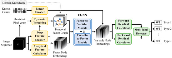
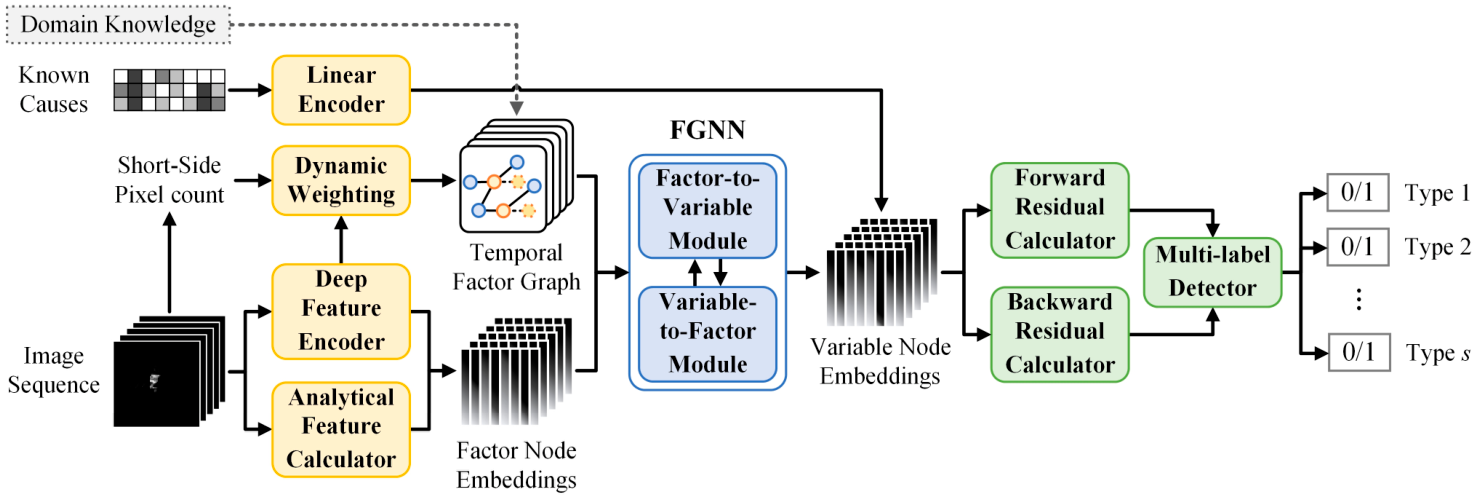
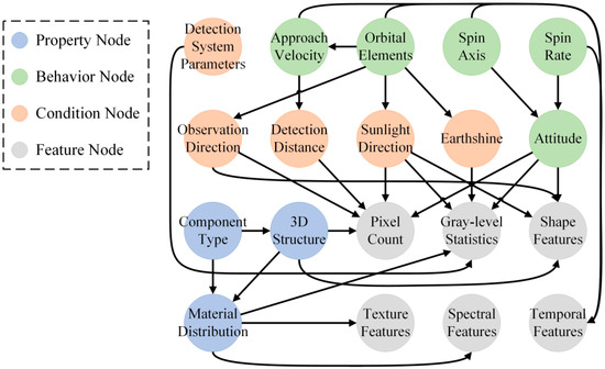
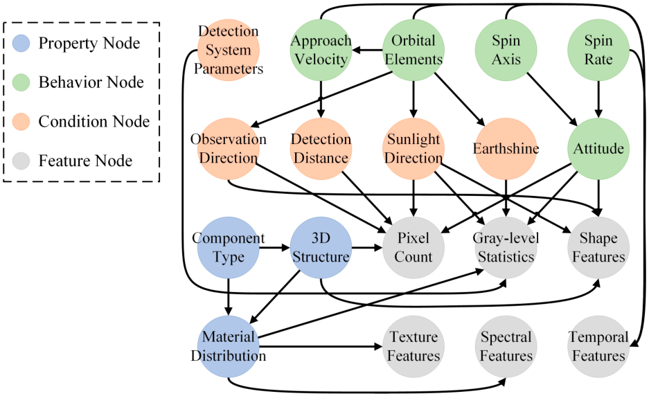
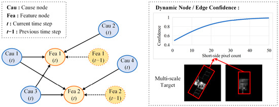
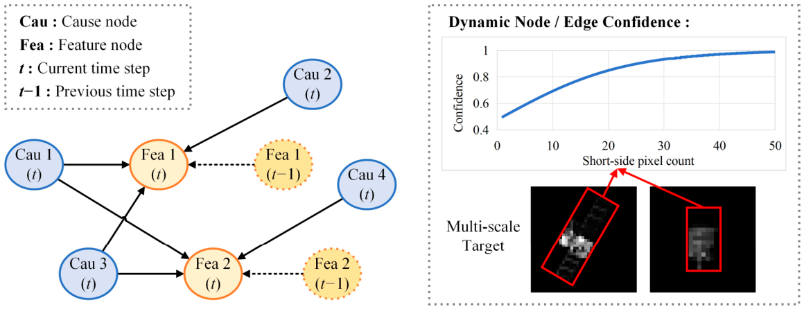
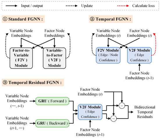
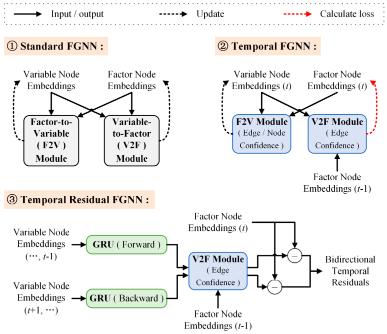
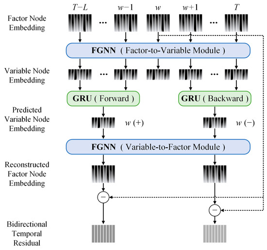
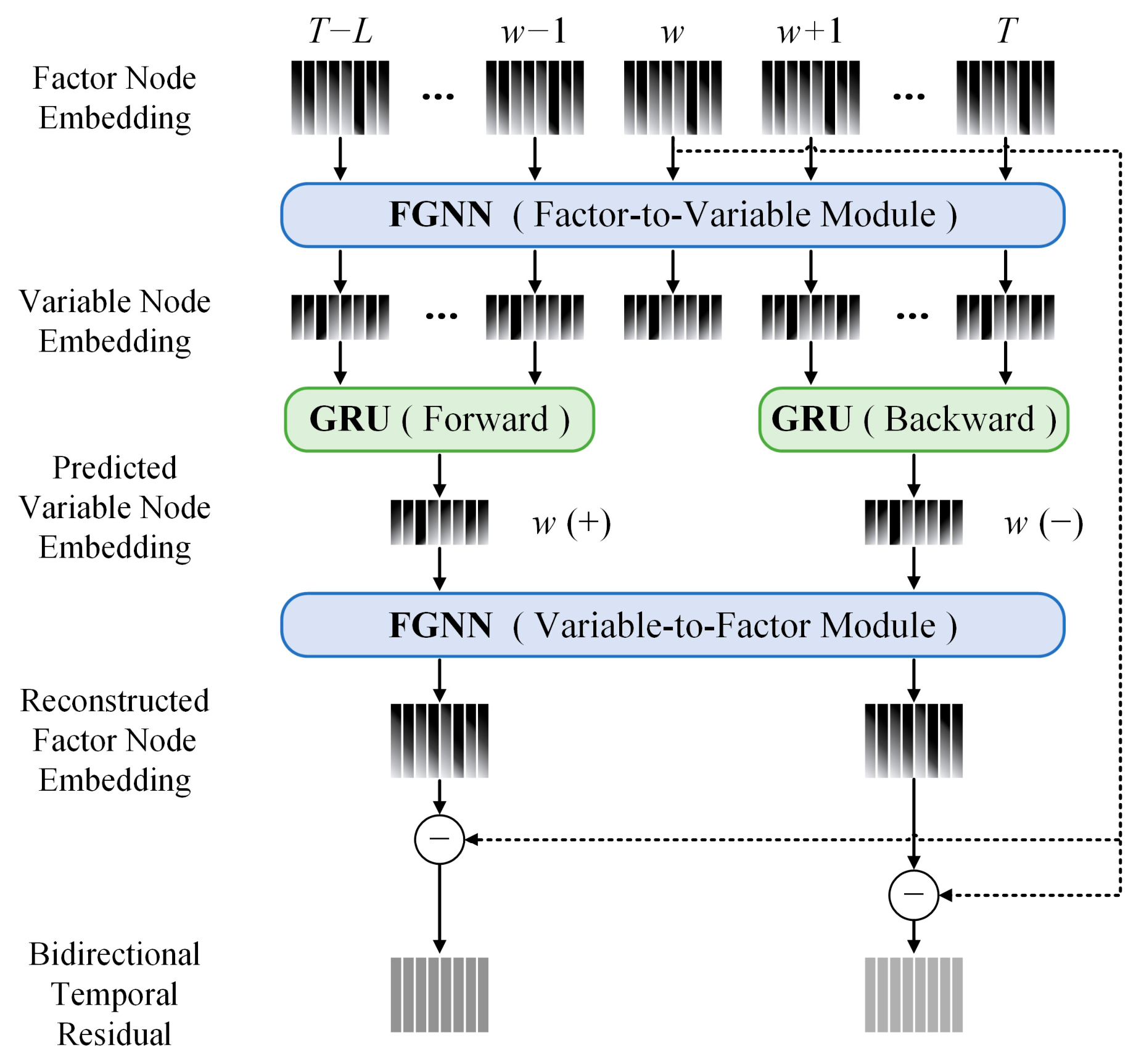
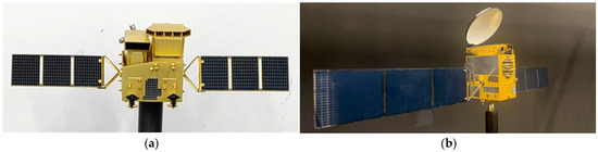
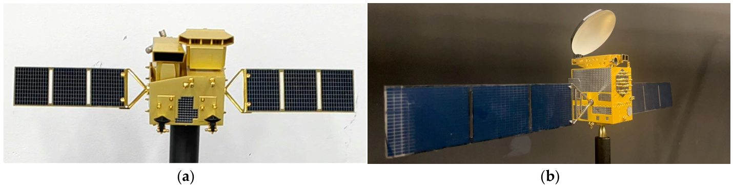
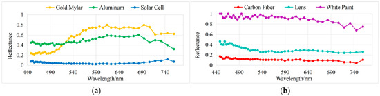
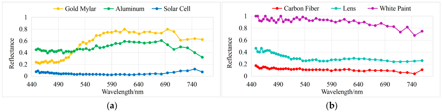
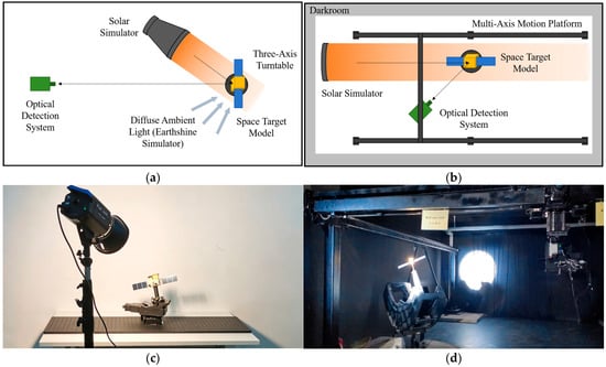
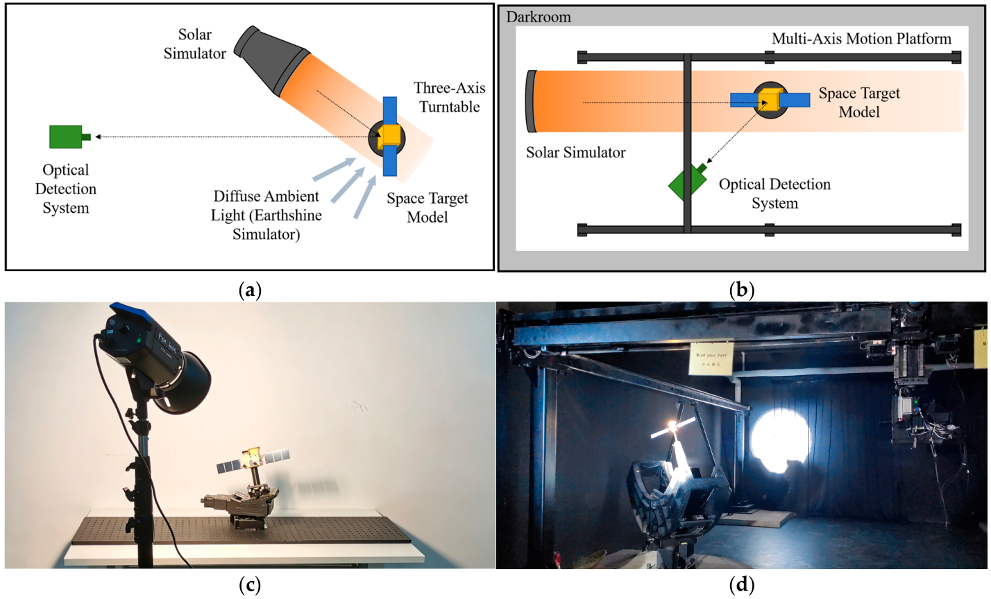
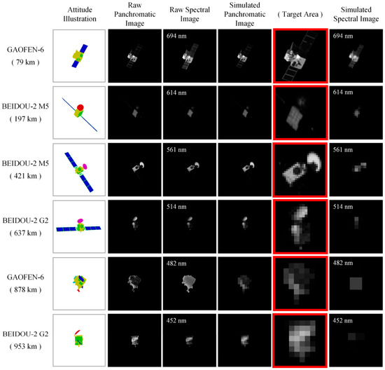
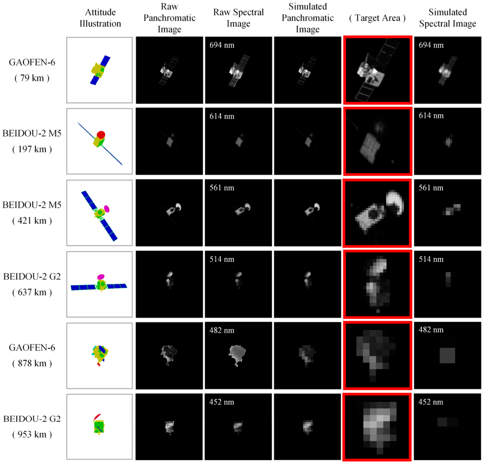
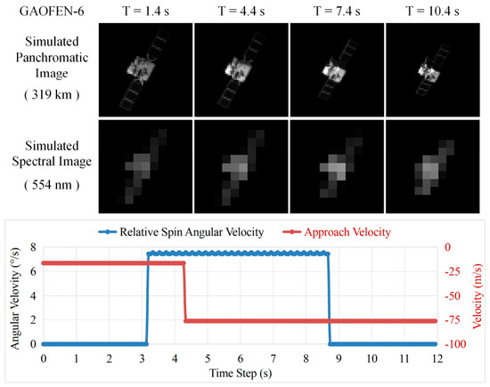
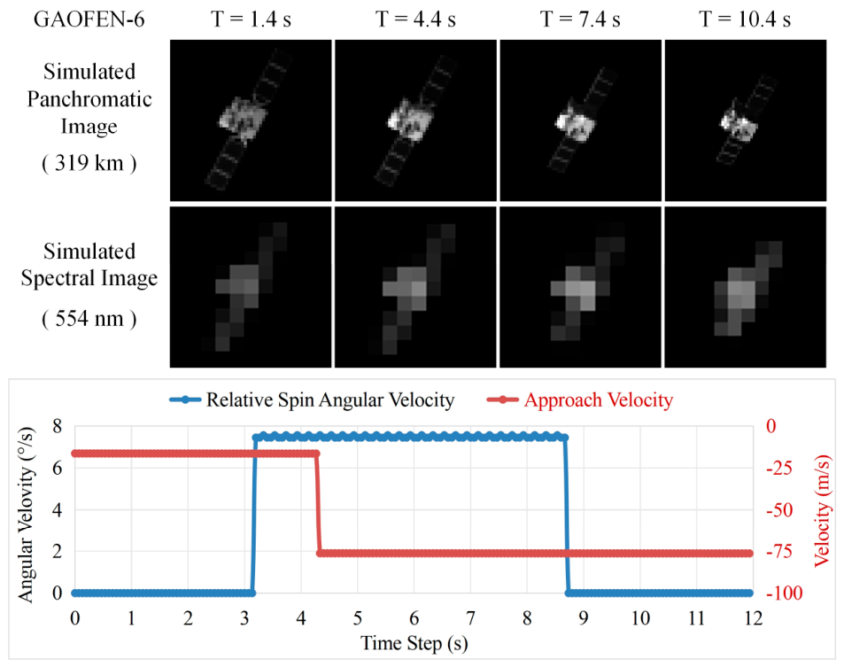
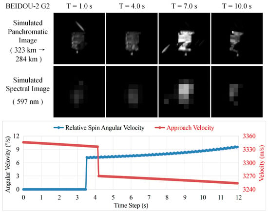
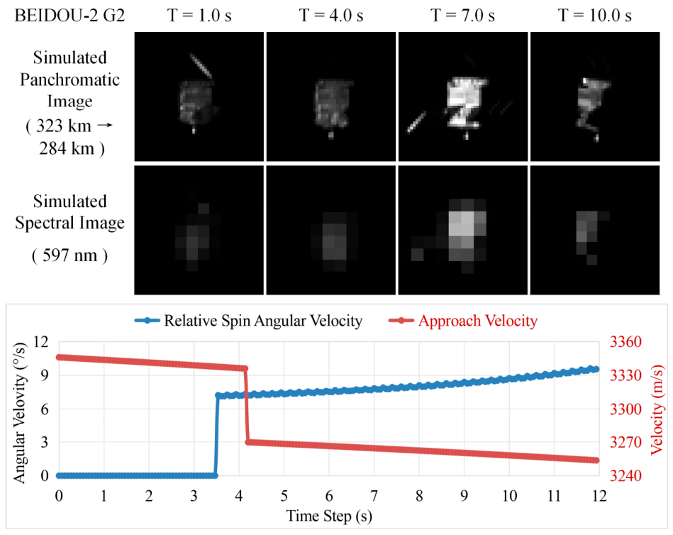
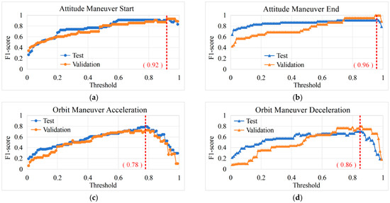
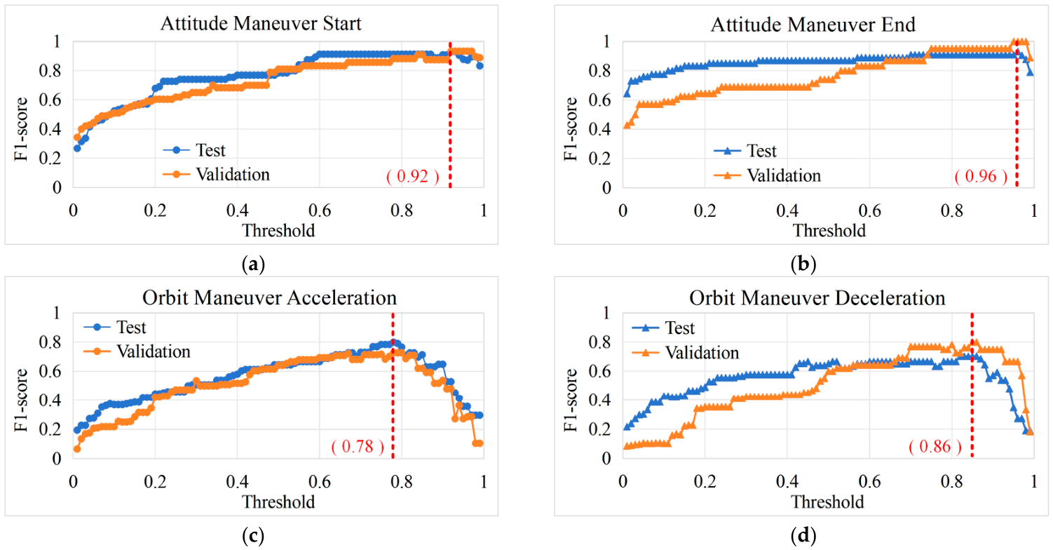
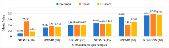
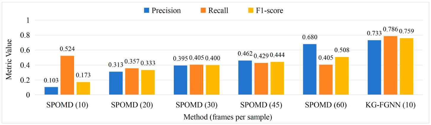
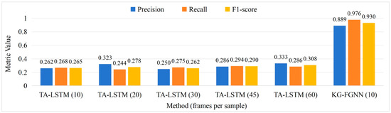
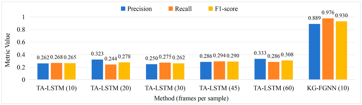
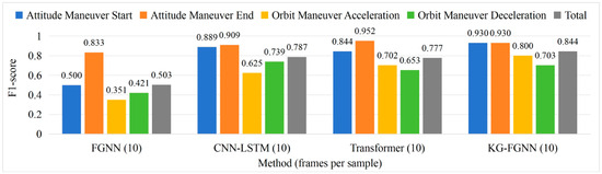
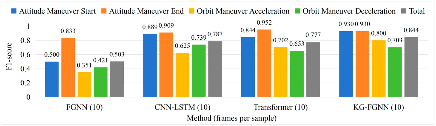
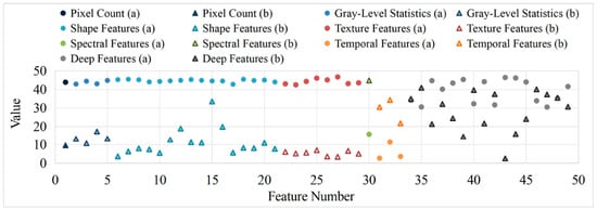
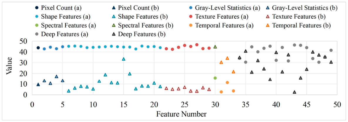
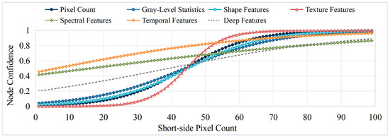
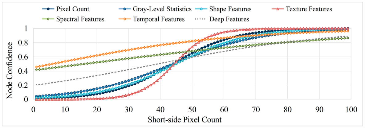
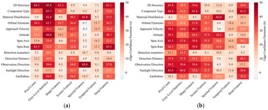
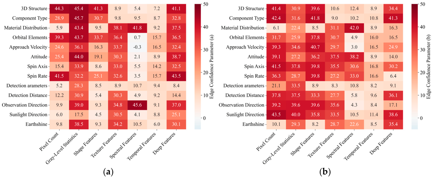
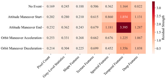
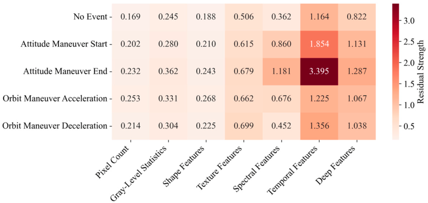
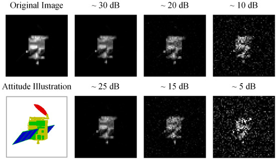
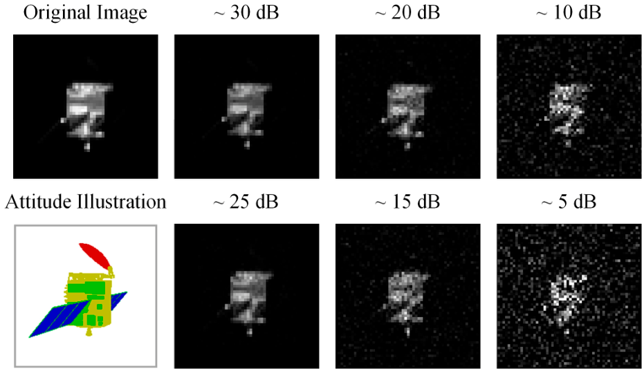
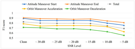
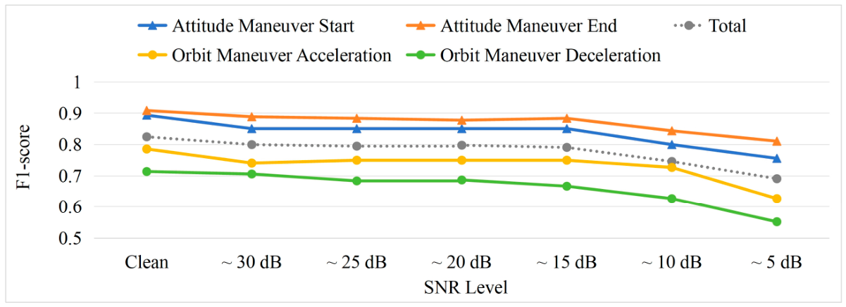
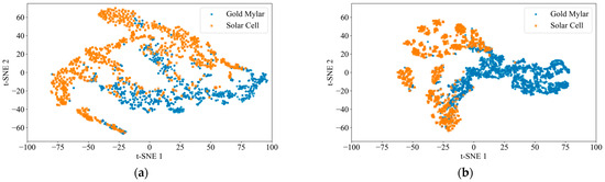
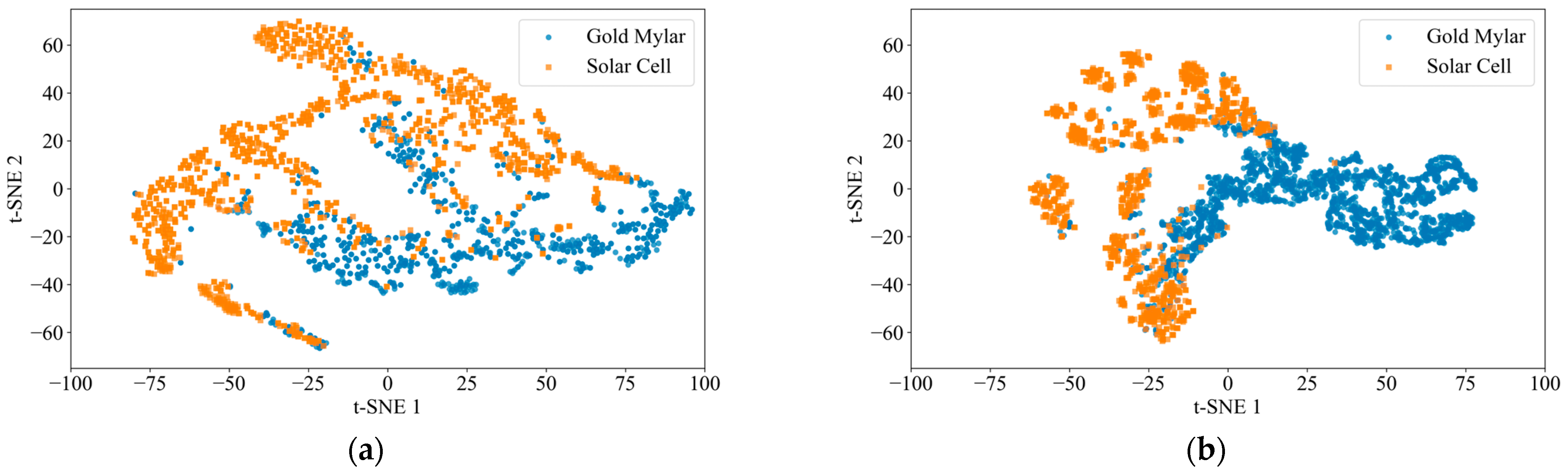
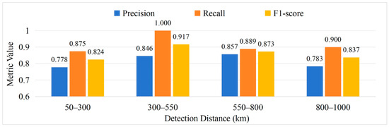
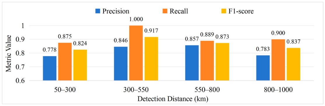
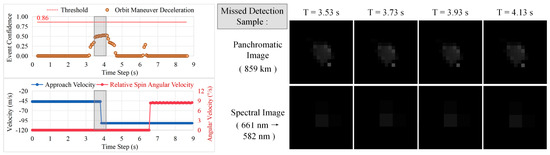
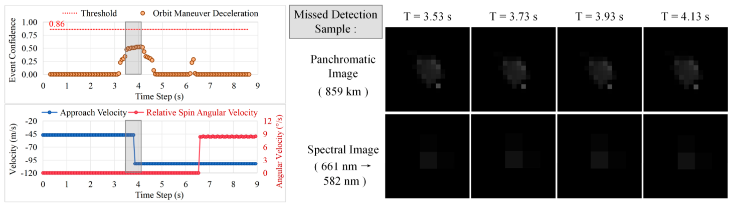
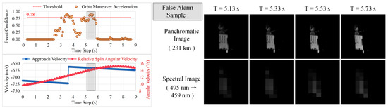
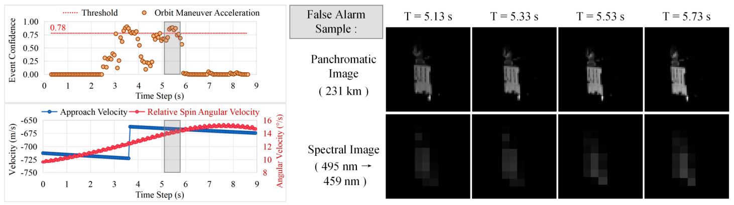
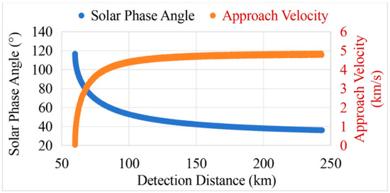
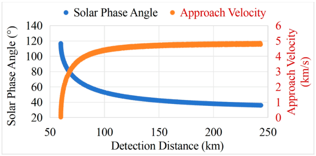

Disclaimer/Publisher’s Note: The statements, opinions and data contained in all publications are solely those of the individual author(s) and contributor(s) and not of MDPI and/or the editor(s). MDPI and/or the editor(s) disclaim responsibility for any injury to people or property resulting from any ideas, methods, instructions or products referred to in the content. |
© 2026 by the authors. Licensee MDPI, Basel, Switzerland. This article is an open access article distributed under the terms and conditions of the Creative Commons Attribution (CC BY) license.