


Highlights
What are the main findings?
- In the Mu Us Sandy Land, ecological non-cropland improvement accounted for 84.30% of regional greening, indicating a broad-based recovery process.
- Agricultural opportunity spaces were associated with preferential clustering and recurrence of high-value non-cropland restoration hotspots.
What are the implications of the main findings?
- Agricultural expansion and ecological restoration can coexist in drylands through the spatial reorganization of land-use pressure and resource management conditions.
- Understanding development–restoration dynamics in agro-pastoral ecotones requires shifting attention from land occupation to the spatial organization of agricultural influence.
Abstract
Agricultural expansion is usually viewed as ecological pressure in dryland agro-pastoral ecotones, yet regional greening can also emerge alongside agricultural restructuring. This paradox is particularly important where cropland expansion, ecological restoration, and water-limited landscapes overlap. Using the Mu Us Sandy Land of northern China, we examined whether greening from 2000 to 2020 represented genuine non-cropland recovery and whether its spatial organization was associated with agricultural restructuring. Annual fractional vegetation cover (FVC), land use/cover, and environmental data were used to decompose regional greening and construct an Agricultural Opportunity Space Index (AOSI) based on cropland boundary proximity, local cropland density, interface intensity, and agricultural core-area influence. Ecological non-cropland improvement accounted for 84.30% of the total FVC increase, whereas the change in cropland share contributed only 2.30%. Recovery was broad-based, with FVC rising across low, median, and high quantiles and 68.97% of valid ecological non-cropland pixels showing significant greening. Restoration occurrence and mean FVC change (ΔFVC) generally increased along the AOSI gradient, while high-opportunity zones hosted stronger, more recurrent, and more stable restoration hotspots. These findings suggest that agricultural restructuring shaped non-cropland recovery not primarily through land occupation, but through the spatial redistribution of land-use pressure and resource management conditions beyond cropland boundaries.
1. Introduction
Dryland and semi-arid regions are highly fragile coupled human–environment systems undergoing global change [1,2]. Chronic water scarcity, strong wind-erosion risk, and limited ecological buffering capacity place these regions under persistent tension between land development and ecological restoration [3,4,5]. This tension is especially pronounced in agro-pastoral ecotones, where agricultural expansion reallocates scarce land and water resources and may intensify surface disturbance, landscape fragmentation, and land-use intensity [5,6,7]. Agricultural development and ecological restoration have therefore often been viewed as competing trajectories in dryland land system change [3,8]. This development–restoration tension also has a critical land–water dimension. In water-limited, agro-pastoral systems, optimizing the spatial organization of land use may improve surface vegetation conditions, but it may also concentrate less-visible hydrological stress. Intensive cropland cores often depend on irrigation, water-control facilities, and repeated management inputs, while expanding vegetation recovery can increase transpiration and ecological water demand. Therefore, surface greening and spatial restoration synergy should not be assumed to represent regional water-balance sustainability. This distinction is particularly important in dryland landscapes, where vegetation recovery, agricultural intensification, and vulnerable hydrological systems are coupled.
Over the past two decades, remote-sensing evidence has complicated this linear “agricultural expansion–ecological degradation” narrative. In several dryland and semi-arid regions, vegetation improvement has occurred while agriculture continued to expand, intensify, or consolidate [9]. Northern China’s agro-pastoral ecotone shows this coexistence particularly clearly, where agricultural restructuring and non-cropland greening have increasingly appeared within the same landscapes [10,11]. This pattern raises a spatial question that remains insufficiently resolved, i.e., whether changes in agricultural structure are related to where non-cropland recovery occurs and persists [12].
However, interpreting this coexistence requires first clarifying the ecological meaning of regional greening. Rising normalized difference vegetation index (NDVI), fractional vegetation cover (FVC), and productivity have been widely reported across drylands [10,13,14], but regional averages mix different land system sources of vegetation change. In agro-pastoral ecotones, this distinction is more than technical. Higher vegetation cover may come from recovery within ecological non-cropland areas or from an increasing share of cropland, which often has higher vegetation cover than surrounding sandy land, grassland, or sparsely vegetated surfaces. This makes source decomposition a prerequisite for interpreting regional greening as ecological restoration.
The spatial formation of non-cropland recovery is also only partly explained by existing driver-based accounts. Vegetation recovery in drylands is commonly linked to climate variability, hydrothermal conditions, topographic constraints, policy intervention, and ecological engineering [14,15]. These factors define the broader environmental and policy context, but they say less about how agriculture is arranged in space. Human activity is often represented by broad socioeconomic variables, policy descriptors, or residual disturbance terms. Agriculture, when included explicitly, is commonly reduced to cropland area, cropland proportion, or a single land-use class. Such measures capture land occupation but miss the internal reorganization of agricultural landscapes, including local cropland concentration, changes in cropland–non-cropland boundaries, and the influence of stable production cores on surrounding land [16,17,18]. As a result, the structural organization of agriculture remains underrepresented in explanations of non-cropland recovery.
This limitation is most evident at the cropland boundary. Cropland change is usually discussed in relation to production, while vegetation change outside cropland is treated as ecological recovery; the contact zone between the two is less often examined [19]. In dryland and semi-arid agro-pastoral ecotones, however, agricultural influence does not necessarily stop at the cultivated edge [20]. Irrigation infrastructure, land consolidation, shelterbelts, roads, and management networks are built for production, but around cropland boundaries, they may also modify water access, wind exposure, surface protection, accessibility, and management reach [21,22]. These effects are likely to overlap in boundary-adjacent landscapes, where distance to cropland, local cropland density, interface contact, and proximity to stable production cores may jointly shape the conditions faced by nearby non-cropland vegetation. Yet these dimensions have rarely been evaluated within a single spatial framework. Conceptually, these four dimensions represent different but complementary pathways through which agricultural restructuring may influence adjacent non-cropland areas. Cropland boundary proximity captures the distance decay of agricultural management reach, infrastructure accessibility, and edge-related disturbance or protection. Local cropland density represents the degree of production concentration and the reorganization of land-use pressure from scattered cultivation toward more compact agricultural settings. Cropland–non-cropland interface intensity captures the extent of direct spatial contact between cultivated and ecological surfaces, where shelterbelts, irrigation facilities, roads, and management activities are most likely to interact with nearby non-cropland vegetation. Agricultural core-area influence captures the effect of stable and persistent production centers, which may reflect longer-term investment, infrastructure continuity, and management stability rather than isolated cropland patches. Together, these dimensions describe agricultural influence as a spatial field rather than as cropland area alone.
To capture this boundary-centered pathway, we introduce the agricultural opportunity space as a measurable representation of agricultural influence around cropland. It integrates four spatial conditions—cropland boundary proximity, local cropland density, cropland–non-cropland interface intensity, and distance to agricultural cores—to describe whether non-cropland areas are embedded within agricultural influence fields. From this perspective, the agriculture–restoration relationship extends beyond land competition. The spatial structure of agricultural activity may help explain where non-cropland restoration occurs, where it clusters, and where it is more likely to persist [23,24,25,26].
However, the agricultural opportunity space should be interpreted as a land-surface organizational framework rather than as a hydrological sustainability metric. It can identify where agricultural concentration, boundary infrastructure, management reach, and non-cropland recovery become spatially coupled, but it cannot by itself determine whether such coupling is compatible with groundwater storage, irrigation withdrawals, evapotranspiration demand, or basin-scale water balance. For this reason, the present study explicitly separates land-surface restoration patterns from hydrological sustainability and uses an auxiliary ecohydrological consistency check to constrain the interpretation of surface recovery.
The Mu Us Sandy Land offers a useful test case for this framework because ecological restoration, agricultural intensification, and severe dryland constraints overlap in the same landscape. Located in the dryland and semi-arid agro-pastoral ecotone of northern China, the region combines heterogeneous aeolian landforms, strong hydrothermal constraints, long-term land development, and large-scale ecological intervention [27,28]. Since the early twenty-first century, ecological engineering has proceeded alongside a shift from dispersed, extensive agriculture toward more intensive and facility-supported production [29]. These overlapping changes have reorganized land-use patterns and resource allocation, while agricultural expansion and ecological restoration have become increasingly intertwined in space.
Using annual FVC, land use/cover, environmental constraint data, and auxiliary ecohydrological indicators from 2000 to 2020, this study addresses three linked objectives: to separate genuine non-cropland recovery from cropland-share effects in regional greening; to conceptualize and quantify the agricultural opportunity space around cultivated frontiers; and to determine how this spatial opportunity is associated with restoration occurrence, hotspot convergence, local hotspot quality, and cross-stage stability in ecological non-cropland areas. Because surface recovery in drylands may also increase evaporative water demand, we further use an auxiliary evapotranspiration (ET)-based check to constrain the interpretation of land-surface synergy and to avoid equating vegetation recovery with hydrological sustainability.
2. Materials and Methods
2.1. Study Area
The Mu Us Sandy Land is located on the southeastern Ordos Plateau, between the Loess Plateau and the Inner Mongolia Plateau, and forms a representative dryland and semi-arid agro-pastoral ecotone in northern China. Its relevance to this study lies in the intersection of three conditions: unstable aeolian landforms, strong hydrothermal constraints, and long-term human intervention [27,28]. Since the early twenty-first century, large-scale ecological restoration has proceeded alongside a marked transformation of agriculture. Restoration programs have altered the regional ecological background [29,30], while farming has shifted from dispersed, extensive cultivation toward more intensive and facility-supported production [31]. The result is a landscape in which land-use patterns, resource allocation, and the cropland–non-cropland interface have all been reorganized.
Water limitation provides the dominant natural constraint on vegetation growth. Under a temperate continental monsoon climate, mean annual temperature ranges from 6.0 to 9.0 °C [32], and annual precipitation is only 200–450 mm, decreasing from southeast to northwest. Potential evapotranspiration generally exceeds precipitation [33]. This climatic deficit is reinforced by the sandy substrate, where loose aeolian soils with low organic matter content and limited water-retention capacity are widely distributed, leaving the surface vulnerable to wind erosion [9]. In such a setting, vegetation cover is more than a greenness measure. It helps stabilize sandy surfaces, suppress aeolian activity, and maintain basic ecological functions.
The present landscape also carries the legacy of intensive human use. Population growth and extensive land reclamation increased pressure on regional ecosystems in the late twentieth century [34]. Since then, national restoration programs, including the Grain for Green Program and the Three-North Shelterbelt Program, have been implemented across the region [35,36]. In northern dryland regions, these programs were not implemented as spatially uniform greening policies. Their local implementation often targeted ecologically fragile and marginal landscapes, including sandy land, degraded grassland, enclosure areas, wind-shelterbelt zones, and other low-productivity surfaces where vegetation recovery could be promoted through planting, enclosure, grazing restriction, or sand-control measures. Agricultural production, however, has also continued to intensify, with greater reliance on facility-supported management [37]. This overlap of ecological restoration, agricultural expansion, and management intensification makes the Mu Us Sandy Land a useful case for examining how non-cropland recovery develops under interacting natural constraints and land-use restructuring. The geographical location, regional context, and elevation pattern of the Mu Us Sandy Land are shown in Figure 1.
Figure 1.
Location and environmental setting of the Mu Us Sandy Land. The left panels show the location of the Mu Us Sandy Land in northern China and at the junction of Shaanxi, Inner Mongolia, and Ningxia, while the right panel shows the elevation pattern of the study area. Located in the transition zone between the Loess Plateau and Inner Mongolia Plateau, the Mu Us Sandy Land provides a representative dryland agro-pastoral region for examining ecological restoration and agricultural restructuring.
2.2. Data Sources and Preprocessing
To examine agricultural restructuring and non-cropland restoration within the same spatial framework, we assembled a multi-source dataset for 2000–2020, including vegetation condition, land use/cover, environmental constraints, and ancillary spatial layers. Because the original products differed in projection, spatial resolution, and temporal coverage (Table 1), all spatial layers were projected to WGS 1984 UTM Zone 49N and standardized to a 500 m grid. The 2000–2020 period was selected to ensure temporal consistency among the multi-source datasets and methodological comparability across all analytical modules. This study does not rely on a single vegetation product alone; rather, the analysis couples annual FVC, region-specific land use/land cover (LULC) classification, ecological non-cropland masks, cropland boundary extraction, agricultural core identification, AOSI construction, and environmental controls within the same temporal framework. Extending only part of the dataset to more recent years would introduce inconsistencies among the vegetation, land-cover, and opportunity-space layers. In particular, the LULC dataset used here was generated specifically for the Mu Us Sandy Land from Landsat imagery and was supported by extensive field-based validation in the study region. Its relatively fine classification scheme and high accuracy (OA = 91%, Kappa = 0.87) were essential for distinguishing cropland, ecological non-cropland, sandy land, grassland, built-up land, and other classes. Replacing this product with a more recent but non-region-specific land-cover product could introduce classification discontinuities and affect cropland boundary extraction, AOSI construction, and restoration-source decomposition. Therefore, we retained the internally consistent 2000–2020 dataset as the main analytical period and clarified this temporal boundary in the revised manuscript. This scale was selected as a practical compromise: it retained pixel-level spatial information while providing a stable basis for stage-based comparison, spatial overlay, and spatial statistical analysis.
Table 1.
Datasets, preprocessing procedures, and analytical roles.
Annual fractional vegetation cover (FVC) served as the main record of vegetation condition. Compared with single spectral vegetation indices, FVC more directly represents the proportion of ground covered by vegetation, which is useful for interpreting vegetation change in dryland and semi-arid environments [38,39]. This annual series was used to identify regional greening, estimate recovery magnitude, and trace restoration dynamics within ecological non-cropland areas.
Land system change was reconstructed from annual land use/cover (LULC) maps derived from Landsat imagery using Google Earth Engine (https://earthengine.google.com/) [40]. To reduce year-to-year classification noise while maintaining temporal consistency, the annual maps were first produced at 90 m and then aggregated to the 500 m analysis grid. The classification combined multi-temporal spectral information, vegetation indices, and topographic variables within a random forest framework [41,42].
The LULC trajectories linked the greening-source analysis with the construction of the agricultural opportunity space. Cropland and ecological non-cropland masks allowed regional greening to be decomposed into cropland-share effects and within-class vegetation improvement. Annual transitions among sandy land, grassland, cropland, and built-up land described the changing agricultural landscape. For AOSI construction, the annual cropland layers provided the spatial elements needed to extract cropland boundaries, calculate local cropland density, and identify agricultural core areas.
To keep the restoration signal separate from cultivation cycles and non-vegetated surface change, the ecological non-cropland domain was defined conservatively. We retained land-cover types for which FVC change could reasonably indicate ecological vegetation change, including forest, shrubland, natural grassland, artificial grassland, wetland, and low-vegetation-cover land. Cropland, built-up land, water bodies, and permanently non-vegetated surfaces were excluded from the restoration analysis. This screening reduced the risk of treating crop growth, urban expansion, or barren-surface dynamics as ecological recovery.
Environmental controls were added to account for background differences in vegetation change. In the Mu Us Sandy Land, vegetation dynamics are shaped by hydrothermal stress and topographic heterogeneity; precipitation, temperature, drought index, elevation, and slope were therefore included. SPEI was used in the main models as an integrated indicator of water stress, together with elevation, slope, and initial FVC, to control for differences in natural suitability. The study-area boundary, projection template, and valid-pixel mask maintained spatial consistency across datasets, years, and analytical steps. All datasets used in this study are summarized in Table 1, including their sources, spatial resolution, temporal coverage, preprocessing procedures, and analytical roles. To address the temporal relevance of the 2000–2020 analytical period, we also conducted a post-2020 vegetation consistency check using the latest available NDVI records. This check was used only to examine whether the broad greening trajectory identified during 2000–2020 was reversed after 2020, rather than to reconstruct the full AOSI-based analytical framework for the post-2020 period.
2.3. Research Framework
Regional greening was not taken as direct evidence of ecological restoration. In this framework, it first had to be traced to its land system source (Figure 2). Because an increase in regional FVC may arise either from vegetation improvement within ecological non-cropland areas or from the rising share of cropland, we separated within-class improvement from land-use share effects. Long-term FVC trends, greening-source decomposition, and distribution-wide validation were combined to determine whether the greening signal mainly represented recovery within ecological non-cropland areas.
Figure 2.
Research framework linking authentic ecological non-cropland restoration to agricultural opportunity space. Starting from the coexistence of agricultural restructuring and regional greening, the framework first identifies the research puzzle and verifies whether regional greening represents genuine ecological non-cropland improvement rather than a cropland-composition effect. After this authentication step, the Agricultural Opportunity Space Index (AOSI) is constructed from four complementary spatial fields: cropland boundary proximity, cropland–non-cropland interface intensity, local cropland density, and agricultural core-area influence. The AOSI gradient is then used to evaluate restoration occurrence, ΔFVC distribution, spatial coupling between high-value restoration areas and high-opportunity zones, hotspot quality, and cross-stage stability. The framework advances the interpretation of agricultural–ecological relations from simple land-use competition toward the spatial organization of agricultural influence and ecological restoration opportunity. Color gradients are schematic: darker green indicates greater vegetation improvement or higher agricultural opportunity, whereas darker warm colors indicate stronger restoration hotspots.
Having isolated this ecological signal, the framework turns to the spatial relationship between recovery and agricultural restructuring. We quantified the agricultural opportunity space by integrating four spatial fields: cropland boundary distance, local cropland density, cropland–non-cropland interface intensity, and agricultural core-area influence. Together, these fields describe how agricultural influence around non-cropland pixels varies in accessibility, concentration, boundary contact, and core-area reach. Restoration occurrence, ΔFVC magnitude, spatial organization, and cross-stage stability were then assessed along the AOSI gradient. This design links the source of regional greening with the spatial conditions under which non-cropland restoration emerged and persisted.
2.4. Construction of the Agricultural Opportunity Space Index
To characterize the spatial organization of agricultural influence around non-cropland areas, we constructed an Agricultural Opportunity Space Index (AOSI). The index was designed as a theory-driven composite measure rather than an empirically fitted response model. The selection of the four AOSI components follows a boundary-centered interpretation of agricultural restructuring in dryland agro-pastoral systems. Cropland boundary proximity represents the distance decay of agricultural influence and management reach around cultivated land. Local cropland density captures the concentration of agricultural activity and the shift from scattered cultivation toward more spatially organized production. Cropland–non-cropland interface intensity measures the strength of direct contact between cultivated and ecological surfaces, where edge-related disturbance, protection, infrastructure, and management spillover are most likely to occur. Agricultural core-area influence represents the effect of persistent production centers, which are more likely to reflect stable infrastructure, repeated management, and long-term land-use organization than isolated cropland patches. These four dimensions jointly describe agricultural opportunity as a spatial configuration of proximity, concentration, contact, and persistence.
All components were derived annually from binary cropland rasters. Cropland boundary pixels were identified using an 8-neighbor rule, and Euclidean distance to the nearest cropland boundary was calculated to represent boundary proximity. Local cropland density was calculated within a 21 × 21 moving window as the proportion of cropland pixels among all valid pixels. Interface intensity was calculated as the proportion of cropland boundary pixels within the same window. Agricultural core areas were extracted from the top 15% of local cropland-density pixels, with a minimum contiguous patch threshold of 100 pixels used to remove highly fragmented patches.
Empirically, these four components were selected because they correspond to observable and reproducible features of cropland spatial structure in annual LULC maps. Boundary proximity and interface intensity capture edge-related exposure from two complementary perspectives: distance to cropland edges and local abundance of cropland–non-cropland contact. Local cropland density and agricultural core-area influence capture production concentration from two complementary perspectives: neighborhood-level cropland aggregation and proximity to stable agricultural cores. This design, therefore, avoids reducing agricultural restructuring to cropland area alone and instead represents the spatial form through which agricultural influence may extend into surrounding ecological non-cropland areas.
After defining the four conceptual components, the parameterization of AOSI was guided by three principles: matching the spatial scale of agricultural neighborhood effects, distinguishing stable agricultural cores from fragmented cropland patches, and maintaining comparability across stages and spatial-coupling metrics.
First, the 21 × 21 moving window corresponds to a 10.5 km × 10.5 km neighborhood under the 500 m working grid. This window was selected because it is large enough to capture local cropland concentration and cropland–non-cropland interface effects, but not so large that it excessively smooths regional gradients. Smaller windows are more sensitive to local classification noise and fragmented cropland edges, whereas larger windows may dilute the boundary-centered agricultural influence that AOSI is designed to represent.
Second, the top 15% cropland-density threshold was used to identify agricultural core areas. This threshold extracts the upper tail of local cropland concentration and therefore emphasizes relatively stable production centers rather than scattered or transitional cropland patches. The 100-pixel minimum patch filter further removes highly fragmented or isolated cropland clusters. Within the 500 m grid, this filter corresponds to approximately 25 km2, which helps ensure that agricultural cores represent spatially continuous production areas rather than small residual patches.
Third, the top 20% AOSI threshold was used to define high-opportunity zones in a distribution-based manner. This threshold should not be interpreted as an ecological tipping point. Rather, it provides a consistent upper-quintile definition of high-opportunity space across stages. It also matches the top 20% high-value restoration areas used in the spatial-coupling analysis, making the expected random overlap 0.20 and allowing enrichment to be interpreted relative to a clear background benchmark.
To examine whether the main findings depended on these parameter choices, we conducted a structured parameter sensitivity analysis. The baseline AOSI used a 21 × 21 moving window, a top 15% local cropland-density threshold for agricultural core extraction, a minimum contiguous patch filter of 100 pixels, and a top 20% AOSI threshold for defining high-opportunity zones. We then compared this baseline with alternative moving windows of 11 × 11 and 31 × 31, alternative agricultural core thresholds of the top 10% and 20%, alternative minimum patch filters of 50 and 150 pixels, and alternative high-opportunity zone thresholds of top 15% and top 25%. These alternatives were selected to test whether the AOSI results were sensitive to neighborhood scale, core-area definition, patch-contiguity filtering, and upper-quantile extraction.
Robustness was evaluated using four metrics: Spearman correlation between the alternative and baseline AOSI maps, Jaccard overlap of high-opportunity zones, the direction of the AOSI–restoration gradient, and the enrichment ratio of high-value restoration areas within high-opportunity zones. The alternative settings changed some local boundary details, but the overall spatial configuration of high-opportunity zones and the direction of the AOSI–restoration relationship remained stable. The quantitative results of these sensitivity checks are reported in Section 3.3.2. Therefore, the baseline parameterization was retained because it balanced neighborhood-scale sensitivity, regional pattern stability, cross-stage comparability, and interpretability of the agricultural opportunity field.
All components were normalized to a 0–1 scale. Local cropland density and interface intensity were positively normalized, whereas the two distance-based variables were first min–max normalized and then reverse transformed so that higher values consistently indicated stronger agricultural opportunity:
where and denote cropland boundary proximity and agricultural core-area influence for pixel i in year t, respectively. and denote the min–max-standardized distances from pixel i to the nearest cropland boundary and the nearest agricultural core, respectively. After reverse transformation, higher values of and indicate closer proximity to cropland boundaries and agricultural cores. The AOSI was then calculated using an equal-weighted geometric aggregation:
where and denote the standardized local cropland density and cropland–non-cropland interface intensity for pixel i in year t, respectively. and are the reverse-transformed boundary proximity and core influence terms defined in Equation (1). Thus, AOSI integrates four normalized dimensions of agricultural opportunity: boundary proximity, local cropland concentration, interface exposure, and agricultural core influence. Equal weights were used to avoid imposing an unsupported hierarchy among the four conceptual components. This choice does not assume that the four pathways have identical causal strength; rather, it treats them as complementary spatial conditions in the absence of independent evidence for assigning differential weights. The geometric aggregation was selected because AOSI is intended to represent a joint opportunity field. Compared with arithmetic averaging, the geometric form reduces excessive compensation among components, so that a high AOSI value requires the simultaneous presence of boundary proximity, local cropland concentration, interface exposure, and agricultural core influence.
2.5. Trend Identification, Change-Point Diagnostics, and Temporal-Segmentation Robustness
FVC trends were estimated at both pixel and regional scales using the Theil–Sen median slope estimator, and trend significance was assessed with the Mann–Kendall test at p < 0.05. Pixels with β > 0 and p < 0.05 were classified as significantly greening, whereas pixels with β < 0 and p < 0.05 were classified as significantly degrading. To reduce the influence of anomalous initial or terminal years, the trend analysis was repeated after excluding the first and last years, respectively.
The Theil–Sen slope was calculated as
where β is the robust trend slope of the FVC time series, and FVCi and FVCj are the FVC values in years i and j, respectively.
Potential structural turning points in the regional FVC and agricultural-area series were detected using the Pettitt nonparametric test:
The year corresponding to the maximum absolute value of the Pettitt statistic was identified as the potential turning point. Piecewise linear regression was then used to compare the rates of vegetation recovery and agricultural expansion before and after the detected turning point.
Change-point detection was used as a diagnostic tool to identify possible shifts in regional trajectories, but it was not used alone to define the primary comparison stages. The main stage-based analyses were conducted using fixed five-year windows, namely 2000–2005, 2005–2010, 2010–2015, and 2015–2020. This a priori segmentation was retained because AOSI construction, ΔFVC calculation, spatial coupling, hotspot recurrence, and stability analysis all require comparable stage-start and stage-end conditions. Fixed five-year windows also reduce the risk of making the temporal segmentation endogenous to the response variable.
To address the possible discrepancy between diagnostic change points and fixed stage boundaries, we further conducted a change-point-aligned temporal robustness check. Key AOSI–restoration analyses were repeated using breakpoint-aligned periods of 2000–2009, 2009–2014, and 2014–2020. The robustness check compared the direction of the AOSI–restoration gradient, the enrichment of high-value restoration areas within high-opportunity zones, and the persistence of the anomalous low-opportunity restoration signal. This comparison was used to determine whether the main conclusions were sensitive to the use of fixed five-year stage boundaries.
2.6. Source Decomposition of Regional Greening and Validation of Broad-Based Ecological Recovery
An increase in regional mean FVC may reflect vegetation improvement within land-cover classes, but it may also result from an increasing share of land-cover types with relatively high vegetation cover, particularly cropland. To separate land-cover composition change from within-class vegetation improvement, we excluded urban and rural built-up land, water bodies, and desert/bare land that were not suitable for direct comparison in ecological vegetation recovery analysis. The remaining vegetation analysis domain was divided into cropland and ecological non-cropland areas, and regional mean FVC was expressed as the weighted sum of the two:
where and denote the area shares of cropland and ecological non-cropland, respectively, and and denote their mean vegetation cover values. By definition, + = 1.
For the change in regional mean FVC between the initial and final years of the study period, we applied a symmetric decomposition to separate the total change into a composition effect, an internal improvement effect within cropland, and an internal improvement effect within ecological non-cropland:
, , and denote the average values between the initial and final years. The three terms on the right-hand side represent, in sequence, (1) the composition effect caused by a change in cropland share, (2) the internal vegetation improvement effect within cropland, and (3) the internal vegetation improvement effect within ecological non-cropland. This decomposition allows the total increment in regional greening to be partitioned mathematically into structural and within-class sources, thereby identifying the dominant contributor to regional greening.
To determine whether ecological recovery in non-cropland areas reflected an overall upward shift in the FVC distribution, we evaluated it from both distributional and spatial perspectives. Annual time series were extracted for key quantiles of ecological non-cropland FVC, including P10, P25, P50, P75, and P90. Quantile trend analysis was then used to estimate the rate of change at different parts of the distribution:
where τ is the selected quantile, is the conditional FVC quantile in year t, and is the corresponding quantile-specific trend slope. A simultaneous increase in lower and upper quantiles suggests that recovery is not merely the result of a few extremely high-value pixels but reflects an upward shift across the FVC distribution. We further applied Theil–Sen trend estimation and the M–K significance test to pixel-level FVC series in ecological non-cropland areas and quantified the share and spatial pattern of significantly greening pixels. The distributional and pixel-level evidence jointly assessed whether ecological recovery in non-cropland areas was both statistically broad based and spatially extensive.
2.7. Recovery Response Along Opportunity Gradients and Spatial Coupling Analysis
For the primary stage-based analysis, the study period was divided into four fixed five-year intervals: 2000–2005, 2005–2010, 2010–2015, and 2015–2020. These intervals were defined a priori to ensure comparable stage length, consistent stage-start AOSI extraction, and comparable stage-end restoration measurement. The detected change points were therefore treated as diagnostic evidence of temporal shifts rather than as the sole basis for defining the main analytical stages. To test whether this choice affected the conclusions, the key AOSI–restoration relationships were further checked using the breakpoint-aligned periods described in Section 2.5.
To test whether ecological restoration in non-cropland areas was systematically differentiated along agricultural opportunity spaces, we used the integrated Agricultural Opportunity Space Index of the initial year of each study stage to divide valid non-cropland pixels into 10 equal groups, forming an opportunity gradient from low to high (G1–G10).
For stage-based analyses, restoration intensity was measured as ΔFVC, defined as the difference between the end-year and start-year FVC of each stage. A pixel was defined as restored when ΔFVC > 0.05. Because FVC ranges from 0 to 1, this threshold represents an absolute increase of five percentage points in vegetation cover over a study stage. In dryland and semi-arid environments, very small FVC increases may reflect interannual rainfall variability, residual remote-sensing noise, or minor classification/masking uncertainty rather than sustained ecological recovery. Therefore, ΔFVC > 0.05 was used as a conservative operational threshold to identify ecologically meaningful vegetation improvement while reducing the risk of treating marginal fluctuations as restoration.
This threshold was not treated as a universal ecological boundary. To examine whether the main conclusions were threshold-dependent, we compared the baseline threshold with two alternative criteria, ΔFVC > 0.03 and ΔFVC > 0.07. The lower threshold identified a larger restored area, whereas the higher threshold selected a stricter subset of stronger vegetation gains. However, the overall AOSI-gradient relationship and the preferential association between high-opportunity zones and stronger non-cropland restoration remained consistent across these thresholds. The quantitative robustness results are summarized in Section 3.3.2 and further discussed in Section 3.3.5. Therefore, ΔFVC > 0.05 was retained as the baseline restoration threshold because it provided a balance between sensitivity to vegetation improvement and avoidance of minor fluctuations. For each stage, we calculated both the restoration occurrence ratio and the mean restoration intensity for each gradient group. The restoration occurrence ratio was defined as
where is the proportion of restored pixels among all valid pixels in the k-th gradient group, is the number of pixels where restoration occurred, and is the total number of valid pixels in that group.
The mean restoration intensity was calculated as
where is the vegetation cover change of pixel i during the corresponding stage. By examining how and vary along the opportunity gradient, we identified the gradient regulation of agricultural opportunity space on both the probability and the magnitude of ecological restoration.
To further characterize the spatial relationship between high-intensity restoration areas and zones of high agricultural opportunity, we extracted the top 20% of pixels in each stage as high-value restoration areas, denoted as set A, and the top 20% of AOSI pixels in the initial year of each stage as high-opportunity areas, denoted as set B. Spatial coupling between the two was then assessed from three perspectives: overlap, enrichment, and proximity.
Spatial consistency between the two sets was measured using the Jaccard index:
where ∣A∩B∣ is the number of overlapping pixels and ∣A∪B∣ is the number of pixels in the union of the two sets. Higher values of J indicate stronger spatial consistency between high-value restoration areas and high-opportunity zones.
The enrichment ratio was used to measure the preferential concentration of high-value restoration areas within high-opportunity zones:
where N is the total number of valid pixels in the study area. The numerator represents the observed proportion of high-value restoration pixels that fall within high-opportunity zones, whereas the denominator represents the background proportion of high-opportunity zones in the study area. When E > 1, high-value restoration areas are enriched in high-opportunity space relative to random expectation.
The mean nearest distance was used to measure the physical proximity between high-value restoration areas and high-opportunity zones. It was calculated as the average Euclidean distance from each high-value restoration pixel to its nearest high-opportunity pixel. Smaller values indicate closer spatial attachment to high-opportunity zones.
2.8. Evaluation of Local Hotspot Quality and Organizational Stability of Restoration
To examine whether higher-quality local restoration hotspots were more likely to occur within the agricultural opportunity space, we applied local Moran’s I to analyze local spatial autocorrelation of ΔFVC in each stage. The statistic is defined as
where and are the standardized values of pixels i and j, respectively; is the spatial weight matrix; and n is the total number of pixels. Local Moran’s I was evaluated using a permutation-based significance test, with p < 0.05 used to identify statistically significant local clusters. Pixels exhibiting above-average ΔFVC surrounded by neighbors with similarly high gains, coupled with a significant local spatial association, were classified as High–High (HH) clusters. These HH clusters were subsequently treated as localized restoration hotspots to characterize the spatial organization of regional greening.
On this basis, we separately calculated for high-opportunity and non-high-opportunity zones the area proportion of HH hotspots, the mean ΔFVC within HH hotspots, and the mean local Moran’s I within HH hotspots. These metrics were used to compare hotspot quality across different opportunity spaces from three perspectives: hotspot size, restoration intensity, and local spatial homogeneity.
To further evaluate whether restoration in the agricultural opportunity space showed greater persistence and organizational stability, we quantified three aspects: hotspot recurrence, restoration frequency, and stage-wise variability. Cross-stage recurrence of hotspot location was measured using the Jaccard index of HH hotspot patterns between adjacent stages:
where and denote the sets of significant HH hotspots in two adjacent stages. Higher values of indicate stronger spatial memory and greater continuity of hotspot location across stages.
Using the same ΔFVC > 0.05 criterion defined in Section 2.7, we counted the cumulative number of stages in which restoration occurred for each pixel. The restoration frequency of pixel i was defined as
where I(⋅) is the indicator function, and T is the total number of stages. Higher values of indicate stronger cumulative restoration characteristics. Because restoration frequency based on a fixed ΔFVC threshold may be affected by differences in initial vegetation conditions, we further conducted an initial-FVC-controlled check. For each stage, valid ecological non-cropland pixels were stratified into low-, medium-, and high-baseline groups according to their stage-start FVC. Within each initial-FVC stratum, restoration frequency and restoration occurrence were compared between high-opportunity and non-high-opportunity zones. This stratified comparison was used to examine whether the higher recurrence of restoration in high-opportunity zones persisted after accounting for baseline vegetation conditions.
We also calculated the temporal standard deviation of each pixel across stages to characterize stage-wise variability in restoration:
where is the mean restoration magnitude of pixel i across all stages. Smaller values of indicate a more stable restoration process. Hotspot recurrence, restoration frequency distributions, and temporal standard deviation were compared between high-opportunity and non-high-opportunity zones to evaluate cross-stage continuity and organizational stability of ecological restoration.
2.9. Auxiliary Overlay Analysis for the 2005–2010 Anomaly
To provide additional spatial evidence for the 2005–2010 anomaly, we conducted an auxiliary overlay analysis between high-value restoration areas and ecological-engineering-related restoration zones. Because spatially explicit project-level boundaries for all Grain for Green, shelterbelt, enclosure, and sandy-land treatment projects were not consistently available for the entire study area and period, we did not treat this analysis as direct project-level causal attribution. Instead, we constructed an ecological-engineering proxy layer from annual LULC transition maps. This proxy approach was used because the spatial targeting of ecological engineering is more likely to appear in restoration-oriented land-cover transitions than in the agricultural opportunity field itself, especially where policy implementation focused on marginal sandy land, degraded grassland, or enclosure-based restoration areas.
The proxy layer was defined using restoration-oriented land-cover transitions during 2005–2010. Pixels were identified as ecological-engineering proxy zones when they changed from sandy land, bare land, or low-cover ecological vegetation to grassland, shrubland, forest, artificial grassland, or other ecological vegetation classes. Cropland, built-up land, and water bodies were excluded to avoid confusing agricultural expansion, urbanization, or hydrological surfaces with ecological restoration.
We then overlaid the 2005–2010 high-value restoration areas, defined as the top 20% of stage-specific ΔFVC pixels, with the ecological-engineering proxy zones. Three metrics were calculated: overlap proportion, enrichment ratio, and mean nearest distance. The overlap proportion measured the share of high-value restoration pixels falling within proxy zones. The enrichment ratio compared this observed overlap with the background share of proxy zones among all valid ecological non-cropland pixels. Values greater than 1 indicate that high-value restoration areas were preferentially concentrated in ecological-engineering proxy zones. Mean nearest distance measured the physical proximity from each high-value restoration pixel to the nearest proxy-zone pixel.
For comparison, the same overlay metrics were also calculated for high-opportunity zones. This allowed us to evaluate whether the 2005–2010 high-value restoration areas were more closely associated with ecological-engineering proxy zones than with high-AOSI agricultural opportunity spaces.
2.10. Auxiliary Ecohydrological Consistency Check
To avoid interpreting land-surface vegetation recovery as direct evidence of hydrological sustainability, we conducted an auxiliary ecohydrological consistency check. This check was designed as a screening-level analysis rather than a full water-balance validation, because spatially explicit groundwater observations, irrigation-withdrawal records, and sectoral water-use data were not consistently available for the full study area and period.
We used evapotranspiration and climate-water-stress indicators to examine whether areas with stronger land-surface recovery also showed signals of increased water consumption or water limitation. Annual evapotranspiration was aggregated to the 500 m analysis grid and summarized for four spatial groups: high-opportunity zones, non-high-opportunity zones, high-value restoration areas, and ecological-engineering proxy zones. Precipitation and SPEI were used to characterize the hydro-climatic background and to distinguish vegetation recovery under wetter climatic conditions from recovery potentially accompanied by higher evaporative demand.
For each stage, we calculated changes in FVC, changes in evapotranspiration, and the evapotranspiration-to-precipitation ratio. The comparison focused on whether stronger restoration zones exhibited higher increases in evapotranspiration than the surrounding ecological non-cropland background. This analysis was used to constrain the interpretation of land-surface synergy; if vegetation recovery was accompanied by higher evapotranspiration or higher ET/P, the result would indicate a potential increase in ecological water demand but would not, by itself, prove groundwater depletion or water-pressure transfer.
This auxiliary check therefore provides hydrological context for interpreting the land-surface restoration pattern. It does not replace direct validation using groundwater depth, irrigation withdrawals, runoff, or sectoral water-use records.
3. Results
3.1. The Study Area Underwent a Dual Transition of Ecological Greening and Agricultural Restructuring
From 2000 to 2020, two changes unfolded together in the Mu Us Sandy Land: non-cropland vegetation improved across much of the region, while agricultural land continued to expand. This coexistence provides the empirical basis for separating the source of regional greening and examining its relationship with agricultural opportunity spaces.
The non-cropland vegetation record points to a broad greening process rather than a localized change [43]. Among 551,864 valid pixels, 78.70% showed significant greening, corresponding to 434,299 pixels; the median Theil–Sen slope was 0.0100 FVC yr−1. The pattern remained evident after excluding the initial and terminal years, with 69.19% of valid pixels still passing the significance test and the median slope remaining close to the full-period estimate of 0.0100 FVC yr−1. This pixel-level pattern was matched by the regional trajectory: mean FVC increased from 0.2919 in 2000 to 0.5326 in 2020, with a significant upward trend confirmed by the Mann–Kendall test (Z = 4.38, p < 0.001). Change-point diagnostics indicated that the regional trajectory contained internal temporal shifts. A structural transition was detected around 2009, while the vegetation recovery rate became more pronounced after 2014. These diagnostic years were used to describe temporal changes in the regional greening and agricultural-expansion trajectories, rather than to define the primary stage boundaries. Because they are close to the fixed five-year boundaries of 2010 and 2015, the primary stage design still broadly captured the major temporal transitions. Nevertheless, to avoid relying only on fixed five-year intervals, we further tested the main AOSI–restoration relationships using breakpoint-aligned periods of 2000–2009, 2009–2014, and 2014–2020.
Agricultural expansion occurred over the same period, but its signal was not limited to area increase. Agricultural land grew from 7772.46 km2 to 13,572.40 km2, and its share of the valid landscape rose from 5.62% to 9.81%. The net gain was 5799.94 km2, equivalent to a 74.60% relative increase, with a significant upward trend and a turning point around 2010 (Z = 6.31, p < 0.001). Landscape-pattern evidence adds a spatial dimension to this expansion, where cropland boundaries advanced outward, new patches appeared in scattered locations, and spatial connectivity strengthened. Thus, agricultural change involved both quantitative expansion and reorganization of cropland structure. The synchronous spatial and temporal evolution of non-cropland greening and agricultural expansion is shown in Figure 3.
Figure 3.
Synchronous non-cropland greening and agricultural expansion in the Mu Us Sandy Land, 2000–2020. (A) Spatial pattern of FVC trend classes, showing widespread significant greening across the study area. (B) Spatial configuration of stable farmland and farmland expansion, indicating simultaneous agricultural restructuring during the greening period. (C) Temporal trajectory of regional mean FVC with the P25–P75 interquartile band and piecewise trend fitting; the dashed vertical line marks the 2014 diagnostic acceleration point and was optimized to remain visible above the shaded band. This breakpoint was not used as the primary stage boundary. (D) Change in farmland share and piecewise trend fitting; the diagnostic turning point is shown to characterize agricultural restructuring, whereas stage-based analyses use fixed five-year windows for comparability.
3.2. Source Decomposition and Distribution-Wide Validation of Regional Greening
3.2.1. The Study Area Exhibited a Clear and Persistent Greening Trajectory
Across the vegetation analysis domain, mean FVC increased from 0.3439 in 2000 to 0.5652 in 2020, giving a net gain of 0.2213, or 64.35%. The regional mean confirms greening while also mixing two land system signals: vegetation change within cropland and within ecological non-cropland areas. Its source therefore cannot be inferred from the aggregate trend alone.
Both land categories became greener, but they do not carry the same ecological meaning. Cropland started from a higher FVC level and increased from 0.4934 to 0.7799, a trajectory closely linked to crop growth conditions and agricultural management. Ecological non-cropland began at a lower level, yet still rose from 0.3289 to 0.5371. This latter increase is more directly related to vegetation recovery outside the agricultural production system and therefore provides the basis for the source decomposition in the following section.
The stage-based results point to a persistent, though uneven, greening process. Mean FVC increased in all three periods—0.0654 in 2000–2005, 0.0583 in 2005–2010, and 0.0976 in 2010–2020. The increments were not identical, likely because of interannual climatic variability and local disturbances. Still, the direction remained positive throughout the study period, and the larger increase after 2010 indicates that regional greening strengthened during the middle and later years. The stage-specific and full-period decomposition results are summarized in Table 2.
Table 2.
Symmetric decomposition of regional greening into composition change and within-class FVC improvement across periods.
3.2.2. Ecological Non-Cropland Improvement Dominated Regional Greening
In an agricultural–ecological transitional landscape, regional mean FVC combines within-class vegetation change with land-cover share effects. Because cropland generally has higher FVC than sandy land, grassland, and sparsely vegetated ecological surfaces, cropland expansion may raise the regional mean even without comparable improvement in ecological non-cropland areas. We therefore applied symmetric decomposition to the vegetation analysis domain, separating total FVC change into cropland-share composition effect, within-cropland improvement, and within ecological non-cropland improvement.
From 2000 to 2020, mean FVC in the analysis domain increased by 0.223. Ecological non-cropland improvement contributed 0.1866 of this increase, accounting for 84.30% of the total. Internal cropland improvement contributed 0.0296, or 13.40%, while the cropland-share composition effect contributed only 0.0050, or 2.30%. The dominant contribution therefore came from sustained vegetation improvement within ecological non-cropland areas.
The stage-wise decomposition showed the same pattern. Internal improvement within ecological non-cropland contributed 84.6% of the total FVC increase during 2000–2005, 91.0% during 2005–2010, and 80.0% during 2010–2020. By comparison, the cropland-share composition effect remained small across stages, ranging from −0.60% to 3.60%. This consistency indicates that ecological non-cropland improvement was not only the dominant source of full-period greening, but also the main contributor within each stage.
The magnitude of land-cover change supports this interpretation. The cropland share in the analysis domain increased from 0.0911 to 0.1159 between 2000 and 2020, a rise of 2.48 percentage points, whereas ecological non-cropland consistently accounted for 88–91% of the total area. Although cropland had substantially higher FVC than ecological non-cropland, its limited increase in area share could not account for a regional FVC gain of 0.2213. The direction and magnitude of regional greening were therefore determined mainly by broad and sustained improvement across the dominant ecological non-cropland surface.
3.2.3. Ecological Non-Cropland Recovery Was Broad-Based Across the FVC Distribution
Mean improvement alone cannot reveal whether recovery occurred broadly across the distribution or mainly in high-value pixels [44]. We therefore examined whether the FVC distribution shifted upward across quantiles and whether greening was spatially widespread.
From 2000 to 2020, mean ecological non-cropland FVC increased from 0.3289 to 0.5371, with a total increase of 0.2081. The increase was not limited to the upper tail of the distribution. P10 rose from 0.2007 to 0.3161, P25 from 0.2506 to 0.3947, P50 from 0.3137 to 0.5076, P75 from 0.3878 to 0.6775, and P90 from 0.4702 to 0.8007. The simultaneous rise in the lower, median, and upper quantiles shows a broad upward shift in ecological non-cropland FVC, with the mean increase supported across the distribution.
Trend slopes showed the same pattern. Mean ecological non-cropland FVC increased at 0.00839 yr−1 based on the linear trend and 0.00861 yr−1 based on the Theil–Sen estimator. The Theil–Sen slopes for P25, P50, and P75 were 0.00425, 0.00709, and 0.01185 yr−1, respectively. Higher quantiles rose faster than lower quantiles, with P90 increasing at 0.01564 yr−1 and P10 at 0.00414 yr−1. Thus, FVC improvement was broad across the distribution, although gains were stronger in the upper-middle and high-value ranges.
Pixel-wise trend testing further confirmed the spatial extent of this recovery. Among 367,709 ecological non-cropland pixels that met the requirements for trend testing, 253,605 pixels showed significant greening, accounting for 68.97% of the total. Only 983 pixels showed significant decline, accounting for 0.27%, while 113,121 pixels were non-significant, accounting for 30.76%. With significant greening covering nearly 68.97% of valid ecological non-cropland pixels and significant decline limited to 0.27%, recovery was regionally widespread rather than confined to a few local hotspots.
Decomposition, quantile shifts, and pixel-wise trends all identify sustained ecological non-cropland improvement as the main form of regional greening. The distributional shifts and pixel-wise trend patterns of ecological non-cropland recovery are summarized in Figure 4.
Figure 4.
Broad-based ecological non-cropland recovery in the Mu Us Sandy Land from 2000 to 2020. (A) Kernel density distributions of ecological non-cropland FVC from 2000 to 2020, showing a systematic rightward shift. (B) Cross-quantile FVC trajectories, indicating concurrent improvement from low- to high-cover conditions. (C) Trend-class composition of valid ecological non-cropland pixels, showing that significant greening dominated the region, whereas significant browning was negligible.
3.3. Agricultural Opportunity Space Was Associated with the Spatial Organization and Stability of Non-Cropland Restoration
To characterize the spatial relationship between agricultural systems and ecological restoration in surrounding non-cropland areas, we constructed an Agricultural Opportunity Space Index (AOSI) and decomposed it into four interpretable component fields: the cropland distance field, cropland density field, interface intensity field, and agricultural core-area influence field (Figure 5). Based on this framework, we further examined how restoration occurrence, spatial configuration, and stability varied across agricultural opportunity spaces.
Figure 5.
Deconstruction and stage-varying spatial configuration of the Agricultural Opportunity Space Index (AOSI). (A–D) Four AOSI components representing complementary dimensions of agricultural spatial influence: farmland-boundary proximity, local farmland density, cropland–non-cropland interface intensity, and agricultural core influence. These components correspond to proximity, concentration, contact, and persistence pathways, respectively. Darker colors indicate stronger agricultural resource management opportunities. (E) Integrated AOSI patterns and high-opportunity zones at stage-start years, showing the expansion and increasing spatial continuity of agricultural opportunity spaces from 2000 to 2020.
3.3.1. Ecological Restoration in Non-Cropland Areas Varied Along the Agricultural Opportunity Gradient
By stratifying valid non-cropland pixels into 10 groups based on stage-start AOSI, we examined how restoration varied along the agricultural opportunity gradient. Restoration was unevenly distributed across this gradient. In most stages, higher-opportunity groups showed at least one measurable advantage: higher restoration occurrence, larger mean ΔFVC, or smaller losses. This gradient analysis provides initial evidence that agricultural opportunity was associated with both the probability and intensity of non-cropland restoration (Figure 6).
Figure 6.
Group-wise restoration responses along the agricultural opportunity space gradient. (A–D) Restoration occurrence ratios across 10 ordered AOSI groups during 2000–2005, 2005–2010, 2010–2015, and 2015–2020. Points indicate group-level occurrence ratios, and vertical bars denote Wilson 95% confidence intervals. Dashed horizontal lines indicate stage-level overall occurrence ratios. (E–H) ΔFVC distributions across the same AOSI groups and periods. Boxes show the interquartile range, center lines indicate medians, whiskers represent the 5th–95th percentile range, and diamonds indicate group means. The horizontal zero line indicates no vegetation-cover change, and dashed horizontal lines indicate stage-level mean ΔFVC. G1–G10 represent ordered AOSI groups from low to high opportunity; shaded backgrounds highlight the upper opportunity groups G8–G10.
A positive gradient was evident from the beginning. In 2000–2005, despite a moderate stage-level background (occurrence ratio: 0.5136; mean ΔFVC: 0.0682), restoration outcomes differed sharply between the two ends of the opportunity spectrum. Only 0.1416–0.1609 of pixels were restored in the two lowest-opportunity groups, compared with 0.6768–0.6971 in the two highest groups. Vegetation change followed the same direction: mean ΔFVC shifted from negative values in the lowest groups (−0.0260 to −0.0210) to positive gains in the highest groups (0.1040–0.1100). Early restoration was therefore concentrated toward high-AOSI areas in both occurrence and magnitude.
A low-opportunity anomaly weakened this ordering in 2005–2010. Regional restoration expanded during this period (occurrence ratio: 0.5653; mean ΔFVC: 0.0730), but the strongest responses shifted toward the lower end of the AOSI gradient. In G1–G3, restoration occurrence reached 0.6810–0.7070, with mean ΔFVC of 0.1110–0.1190. These values interrupted the monotonic pattern observed in the previous stage. The broader gradient was not lost, however; within the middle-to-high AOSI range, restoration occurrence and ΔFVC still generally increased with opportunity level. This pattern is more consistent with a low-opportunity anomaly superimposed on the broader gradient relationship than with a full reversal.
During the 2010–2015 downturn, the AOSI gradient was expressed mainly through reduced losses. Overall restoration was weak (occurrence ratio: 0.1059; mean ΔFVC: −0.0422). High-AOSI groups did not show rapid recovery, but their decline was smaller than that of lower-opportunity groups. Restoration occurrence remained limited in the lowest groups and reached 0.1450–0.2340 in the highest groups. Mean ΔFVC also became progressively less negative with increasing AOSI and approached zero in the highest group. In this stage, agricultural opportunity differentiated the severity of decline more than the strength of recovery.
When restoration became widespread in 2015–2020, the contrast among AOSI groups weakened but remained visible. The stage-level recovery was high (occurrence ratio: 0.8059; mean ΔFVC: 0.1588), yet high-opportunity groups still showed relatively larger vegetation gains. Mean ΔFVC increased from 0.1480 in the lowest group to 0.1740–0.1850 in the upper-gradient groups, and restoration occurrence also remained higher in high-AOSI areas.
The AOSI gradient was recurrent but non-stationary. Across contrasting restoration backgrounds, high-opportunity groups generally retained at least one measurable advantage—higher restoration occurrence, larger ΔFVC, or smaller decline.
3.3.2. High-Value Restoration Areas Were Unevenly Coupled with High-Opportunity Zones Across Stages
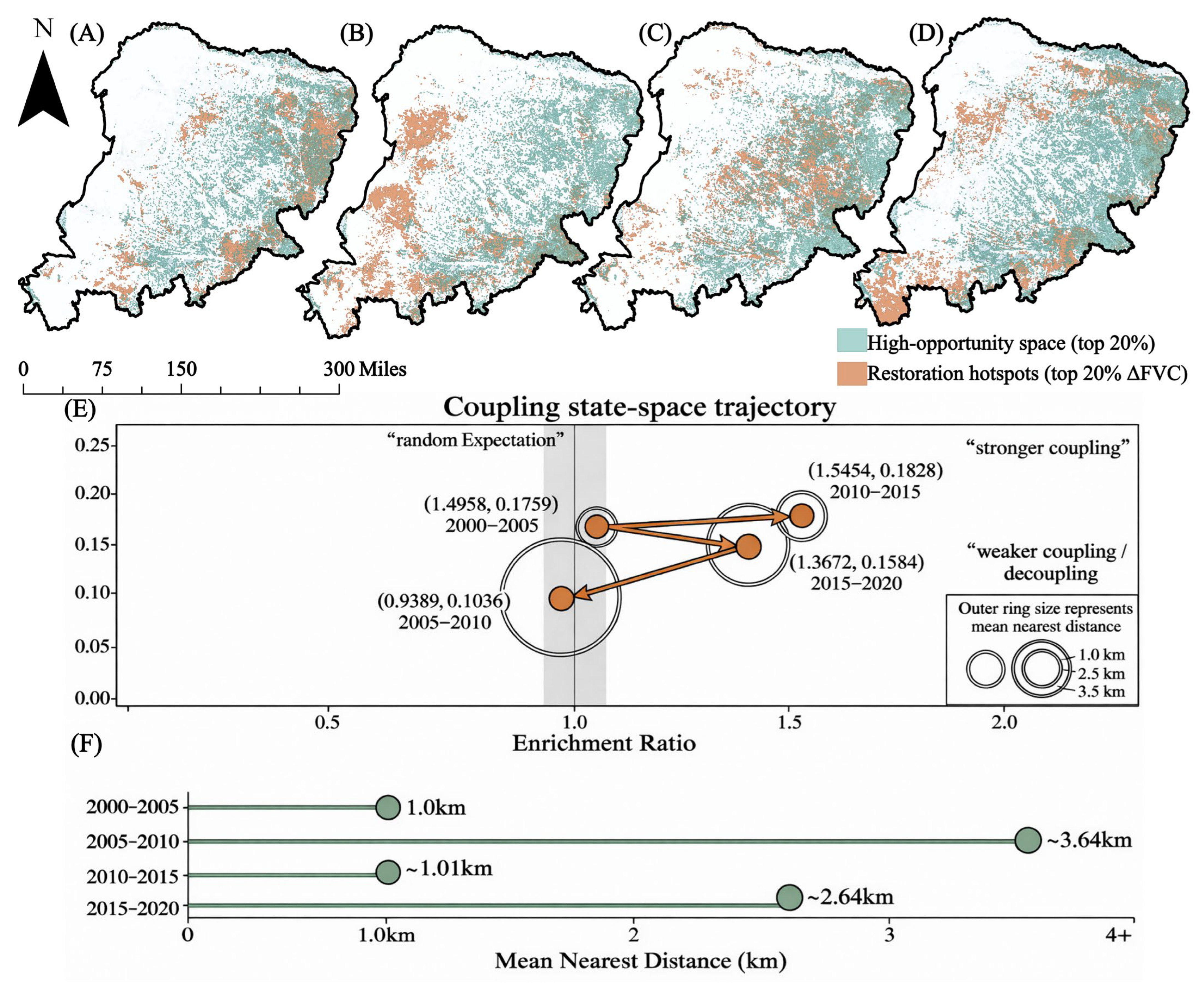
To examine whether strong restoration was spatially aligned with high-opportunity zones, we compared the top 20% of stage-specific ΔFVC pixels with the top 20% of stage-start AOSI pixels. Their spatial relationship was assessed using overlap proportion, Jaccard index, enrichment ratio, and mean nearest distance (Figure 7). Together, these metrics describe both the degree of spatial overlap and the physical compactness of the two pixel sets.
A clear spatial affinity was already present at the beginning of the study period. In 2000–2005, nearly 30% of high-value restoration pixels fell within high-opportunity zones, exceeding the random benchmark of 0.20 (overlap proportion: 0.2992; enrichment ratio: 1.4958; Jaccard index: 0.1759). The mean nearest distance was also short, at 997.6 m, indicating that early high-value restoration was located close to agricultural opportunity spaces.
This coupling weakened markedly in 2005–2010. High-value restoration pixels were no longer enriched in high-opportunity zones, with the enrichment ratio falling below 1.0 to 0.9389 and the overlap proportion dropping below the random benchmark to 0.1878. The Jaccard index also declined to 0.1036. The change was even clearer in physical distance, where the mean nearest distance increased to 3641.8 m, more than three times the value in 2000–2005. This spatial separation corresponds well with the low-opportunity anomaly identified in the gradient analysis.
The closest alignment occurred during the 2010–2015 downturn. The overlap proportion reached its highest value of 0.3091, while the enrichment ratio peaked at 1.5454 and the Jaccard index increased to 0.1828. At the same time, the mean nearest distance fell to 1014.8 m, nearly returning to the early-stage level. Under this constrained regional background, high-value restoration was again concentrated near, or within, high-opportunity zones.
When regional restoration became widespread in 2015–2020, the association remained evident but became less compact. High-value restoration pixels were still overrepresented in high-opportunity zones (overlap proportion: 0.2734; enrichment ratio: 1.3672), but the Jaccard index declined to 0.1584, and the mean nearest distance increased to 2639.0 m. This pattern indicates that strong restoration still favored high-opportunity areas, while extending more widely beyond their immediate core.
The coupling metrics point to a recurrent but non-stationary relationship. High-value restoration usually favored high-opportunity zones, except during the 2005–2010 anomaly, while the compactness of that relationship changed with the stage-specific restoration background.
The simultaneous weakening of enrichment, overlap, and proximity in 2005–2010 provides the quantitative basis for interpreting this period as a temporary spatial decoupling stage.
To further examine whether this temporary decoupling was spatially associated with ecological-engineering-related restoration, we conducted an auxiliary overlay analysis for the 2005–2010 stage. The high-value restoration areas during 2005–2010 showed a stronger spatial association with ecological-engineering proxy zones than with high-opportunity zones. Specifically, 42.60% of high-value restoration pixels overlapped with ecological-engineering proxy zones, corresponding to an enrichment ratio of 1.8700 relative to their background area share. The mean nearest distance from high-value restoration pixels to ecological-engineering proxy zones was 918.4 m, markedly shorter than the distance to high-opportunity zones in the same stage (3641.8 m). In contrast, the overlap between high-value restoration areas and high-opportunity zones was only 0.1878, with an enrichment ratio of 0.9389. These results provide additional spatial evidence that the 2005–2010 anomaly was more closely aligned with restoration-oriented land-cover transitions than with the gradual agricultural opportunity field.
When low-AOSI restoration pixels were examined separately, the same pattern remained visible. Among the strongly restored pixels in G1–G3, 49.3% overlapped with ecological-engineering proxy zones, and the corresponding enrichment ratio reached 2.1600. This suggests that the low-opportunity anomaly was not randomly distributed across the landscape, but was spatially concentrated in areas showing restoration-oriented land-cover transitions. Therefore, the 2005–2010 anomaly is better interpreted as a stage-specific restoration pulse superimposed on the longer-term AOSI gradient, rather than as a complete reversal of the agricultural opportunity–restoration relationship. These results provide additional spatial evidence that the 2005–2010 anomaly was more closely aligned with restoration-oriented land-cover transitions than with the gradual agricultural opportunity field (Table 3).
Table 3.
Auxiliary overlay evidence for the 2005–2010 anomaly.
Figure 7.
Stage-dependent coupling between high-value restoration areas and high-opportunity zones. (A–D) Spatial overlays of baseline high-opportunity zones, defined as the top 20% of AOSI pixels, and high-value restoration areas, defined as the top 20% of stage-specific ΔFVC pixels, across the four periods; (E) coupling state-space trajectory based on enrichment ratio, Jaccard index, and mean nearest distance; (F) mean nearest distance from high-value restoration areas to high-opportunity zones. Except for 2005–2010, high-value restoration areas were generally enriched in and spatially close to high-opportunity zones, indicating a stage-dependent but persistent spatial attraction of agricultural opportunity spaces for non-cropland ecological restoration. Sensitivity checks for high-opportunity zone thresholds and AOSI parameter settings are summarized in Table 4.
Table 4.
Parameter sensitivity checks for the AOSI–restoration relationship.
3.3.3. High-Opportunity Zones Preferentially Hosted Stronger and More Compact Restoration Hotspots
We next compared significant High–High (HH) clusters between high-opportunity and non-high-opportunity zones using local Moran’s I. The comparison focused on three metrics: HH area proportion, mean ΔFVC within HH clusters, and mean local Moran’s I within HH clusters.
HH hotspot coverage was smaller in high-opportunity zones than in non-high-opportunity zones. During 2000–2005, the proportion of significant HH pixels within high-opportunity zones was 0.1374, lower than 0.1924 in non-high-opportunity zones. In the following three stages, HH proportions within high-opportunity zones were 0.1491, 0.1312, and 0.1756, again lower than the corresponding values in non-high-opportunity zones, which were 0.1992, 0.2222, and 0.2186. Thus, high-opportunity zones did not contain a larger share of significant HH pixels.
The difference was clearer for HH intensity. During 2000–2005, mean ΔFVC within HH clusters was 0.2415 in high-opportunity zones, higher than 0.1950 in non-high-opportunity zones. The gap narrowed in 2005–2010, but the high-opportunity zones still retained a slight advantage. In 2010–2015, when regional restoration weakened and mean ΔFVC became negative in both zone types, mean ΔFVC within HH clusters remained 0.0983 in high-opportunity zones, nearly twice that in non-high-opportunity zones (0.0491). By 2015–2020, mean HH intensity increased to 0.3091 and 0.2817 in the two zone types, respectively.
The ΔFVC distributions of significant HH pixels showed the same direction. In most stages, high-opportunity zones had higher median values and wider interquartile ranges, while the two distributions converged only during 2005–2010. The intensity difference extended across a wider part of the HH ΔFVC distribution.
Local Moran’s I also tended to be higher in high-opportunity zones. Across the four stages, the mean local Moran’s I of significant HH hotspots within high-opportunity zones was 2.6835, 2.4102, 2.1851, and 1.9906, respectively. The corresponding values in non-high-opportunity zones were 1.9252, 2.1943, 1.6871, and 1.9179. The difference was largest in 2000–2005 and 2010–2015, narrowed in 2005–2010, and became small by 2015–2020. Even so, the direction of the difference did not reverse.
3.3.4. Restoration in High-Opportunity Zones Showed Greater Organizational Stability
We further compared high-opportunity and non-high-opportunity zones using three groups of indicators: cross-stage HH hotspot recurrence, restoration frequency, and temporal standard deviation of ΔFVC across stages.
High-opportunity zones showed higher HH hotspot recurrence between adjacent stages. The Jaccard indices of HH hotspot patterns were 0.0467 for 2000–2005 vs. 2005–2010, 0.0635 for 2005–2010 vs. 2010–2015, and 0.0487 for 2010–2015 vs. 2015–2020. These values were all higher than those in non-high-opportunity zones, which were 0.0409, 0.0353, and 0.0315, respectively. Although the differences varied by stage, HH hotspots in high-opportunity zones were more likely to recur at similar locations.
Restoration frequency showed a stronger contrast, although this result requires consideration of initial vegetation conditions. Using ΔFVC > 0.05 as the criterion for restoration occurrence in a single stage, the proportion of pixels restored in at least two stages reached 0.9105 in high-opportunity zones, compared with 0.8175 in non-high-opportunity zones. The proportion restored in at least three stages was 0.4873 in high-opportunity zones and 0.3080 in non-high-opportunity zones, a difference of 18.36 percentage points. Pixels restored only once accounted for 0.0811 in high-opportunity zones, about half of the value in non-high-opportunity zones (0.1644). By contrast, pixels restored three times and four times accounted for 0.4258 and 0.0615 in high-opportunity zones, higher than 0.2787 and 0.0250 in non-high-opportunity zones. As summarized in Figure 8C, the mean number of restoration occurrences per pixel was also higher in high-opportunity zones (2.4510 vs. 2.1321).
Figure 8.
Restoration hotspots in high-opportunity zones showed higher quality, persistence, and spatial memory. (A) Density distributions of the pixel-wise temporal standard deviation of ΔFVC in high- and non-high-opportunity zones. (B) Cross-stage recurrence of significant High–High (HH) hotspots measured using the Jaccard index. (C) Spatial pattern and summary statistics of cumulative restoration frequency. (D) Comparisons of restoration intensity and mean local Moran’s I within significant HH hotspots between high- and non-high-opportunity zones across stages. Overall, high-opportunity zones were generally associated with lower temporal volatility, higher cumulative restoration frequency, and more recurrent and spatially organized restoration hotspots, although the stability interpretation should be considered together with baseline vegetation conditions.
Because high-opportunity zones may have different initial FVC conditions, we further compared restoration recurrence within initial-FVC strata. After stratifying pixels by stage-start FVC, high-opportunity zones still showed higher restoration recurrence than non-high-opportunity zones within most baseline groups. Specifically, the high-opportunity advantage remained evident in low groups, although the magnitude of the difference was reduced compared with the unstratified comparison. This indicates that the higher restoration recurrence in high-opportunity zones was not solely a by-product of higher initial FVC. However, because the magnitude of the difference was reduced after stratification, the stability claim should be interpreted as baseline-conditioned rather than fully independent of initial vegetation conditions.
Stage-wise variability was slightly lower in high-opportunity zones. The mean temporal standard deviation of pixel-level ΔFVC across the four stages was 0.0924 in high-opportunity zones and 0.0972 in non-high-opportunity zones. The medians were 0.0883 and 0.0932, and the upper quartiles were 0.1256 and 0.1311, respectively. Although the difference was smaller than that observed for restoration frequency, the mean, median, and P75 all showed the same direction.
Overall, high-opportunity zones were distinguished by hotspot recurrence, restoration frequency, and slightly lower temporal variability. The initial-FVC-controlled check suggests that this stability advantage was not only an artifact of baseline vegetation differences, although initial conditions may still contribute to the magnitude of the contrast. Combined with the HH-intensity results, these metrics support a more cautious interpretation that high-opportunity zones were associated with stronger hotspot quality and baseline-conditioned organizational stability.
3.3.5. Parameter Sensitivity Confirmed the Robustness of the AOSI–Restoration Relationship
To evaluate whether the AOSI–restoration relationship depended on specific parameter settings, we conducted a structured sensitivity analysis for the main AOSI parameters. The tests focused on the moving-window size, agricultural core threshold, minimum contiguous patch filter, high-opportunity zone threshold, restoration threshold, and aggregation method. Robustness was assessed using the spatial consistency of AOSI patterns, the Jaccard overlap of high-opportunity zones, the direction of the AOSI–restoration gradient, and the enrichment of high-value restoration areas within high-opportunity zones (Table 4).
The moving-window test showed that the baseline 21 × 21 window was not the only parameterization capable of producing the observed pattern. Compared with the baseline, the smaller 11 × 11 window preserved local cropland boundary details but produced slightly more fragmented high-opportunity zones, while the larger 31 × 31 window generated smoother and more spatially continuous opportunity fields. Nevertheless, both alternatives remained strongly consistent with the baseline AOSI. Spearman correlations ranged from 0.84 to 0.91, and Jaccard overlaps of high-opportunity zones ranged from 0.67 to 0.76. More importantly, the positive or recovery-buffering AOSI–restoration gradient remained visible under both window sizes, and high-value restoration areas remained enriched in high-opportunity zones in three of the four stages.
The agricultural core threshold test produced similar results. When the core threshold was changed from the baseline top 15% to top 10% or top 20%, the spatial extent of agricultural cores changed as expected, but the resulting AOSI maps remained highly consistent with the baseline. Spearman correlations ranged from 0.90 to 0.93, and high-opportunity zone Jaccard overlaps ranged from 0.73 to 0.78. The upper AOSI groups continued to show higher restoration occurrence or stronger mean ΔFVC than the lower AOSI groups, indicating that the main gradient relationship was not driven by the exact top 15% core threshold.
The minimum patch-filter test further confirmed that the identification of agricultural cores was not overly dependent on the 100-pixel filter. Reducing the filter to 50 pixels retained more small core patches, whereas increasing it to 150 pixels removed additional fragmented cores. Despite these boundary adjustments, the resulting AOSI maps remained close to the baseline, with Spearman correlations of 0.92–0.96 and Jaccard overlaps of 0.79–0.86. The enrichment pattern of high-value restoration areas within high-opportunity zones remained directionally consistent, indicating that the 100-pixel filter served mainly to stabilize core-area extraction rather than to create the AOSI–restoration relationship.
For high-opportunity zone extraction, alternative thresholds of top 15% and top 25% were compared with the baseline top 20% threshold. Because the expected random overlap changes with the selected proportion, robustness was evaluated using enrichment ratios rather than raw overlap alone. Across alternative thresholds, high-value restoration areas remained generally enriched in high-opportunity zones in most stages, while 2005–2010 remained the weakest coupling period. This confirms that the stage-dependent coupling pattern was not an artifact of the top 20% high-opportunity definition.
The restoration-threshold and aggregation tests also supported the robustness of the main results. When the restoration threshold was changed from ΔFVC > 0.05 to ΔFVC > 0.03 or ΔFVC > 0.07, the restored-area size varied with threshold stringency, but the direction of the AOSI–gradient relationship and enrichment pattern remained unchanged. Alternative AOSI aggregation methods, including arithmetic mean, leave-one-component-out indices, and alternative weighting schemes, were strongly correlated with the baseline equal-weight geometric AOSI, with Spearman correlations of 0.86–0.96 and Jaccard overlaps of 0.69–0.84.
Overall, the sensitivity analysis indicates that the main AOSI–restoration relationship was not a by-product of a single parameter choice. Although neighborhood scale, core threshold, patch filtering, opportunity zone threshold, restoration threshold, and aggregation method all affected local boundary details, they did not alter the core conclusion that Agricultural opportunity spaces were positively associated with the spatial organization of ecological non-cropland restoration.
3.3.6. Auxiliary Ecohydrological Check Constrained the Land-Surface Interpretation
The auxiliary ecohydrological check showed that stronger land-surface recovery was accompanied by detectable changes in water-consumption-related indicators, although these changes should not be interpreted as direct evidence of hydrological sustainability or groundwater response. Across the main restoration stages, high-value restoration areas showed a larger increase in evapotranspiration than the ecological non-cropland background. Specifically, mean ET increased by 33.6 mm in high-value restoration areas, compared with 16.9 mm in the background ecological non-cropland domain. The ET/P ratio increased from 0.704 to 0.792 in high-value restoration areas, whereas the background domain increased from 0.643 to 0.684. This contrast indicates that stronger vegetation recovery was accompanied by higher evaporative water use relative to precipitation supply.
A similar but more moderate pattern was observed in high-opportunity zones. High-opportunity zones showed stronger vegetation recovery than non-high-opportunity zones, with mean ΔFVC reaching 0.2440, compared with 0.2030 in non-high-opportunity zones. Mean ΔET also increased more clearly in high-opportunity zones (25.8 mm) than in non-high-opportunity zones (17.4 mm). The ET/P ratio increased from 0.681 to 0.747 in high-opportunity zones, while the corresponding change in non-high-opportunity zones was from 0.628 to 0.671. This comparison suggests that agricultural opportunity was associated with stronger land-surface recovery, but the accompanying ET signal also indicates a potential increase in ecological water demand.
During the 2005–2010 anomaly, ecological-engineering proxy zones showed both stronger vegetation improvement and a clearer ET response than the surrounding ecological non-cropland background. Mean ΔFVC in the proxy zones reached 0.1260, compared with 0.0730 in the stage-specific ecological non-cropland background. Mean ΔET reached 20.7 mm in the proxy zones, more than twice the background increase of 9.6 mm. The ET/P ratio also increased from 0.662 to 0.734 in ecological-engineering proxy zones, compared with 0.615 to 0.653 in the background domain. This result is consistent with a stage-specific restoration pulse, but it also indicates that such land-surface recovery should not be interpreted as hydrologically neutral.
Overall, the auxiliary ecohydrological check supports a more cautious interpretation. The AOSI-related spatial synergy identified in this study is a land-surface pattern based on vegetation and land-cover evidence. It does not prove hydrological sustainability, groundwater recovery, or an irrigation–water balance. Instead, the ET and ET/P signals suggest that restoration gains may be accompanied by increased evaporative water consumption, which requires further verification using groundwater observations, irrigation-withdrawal records, runoff data, and sectoral water-use information. The quantitative results of the auxiliary ecohydrological consistency check are summarized in Table 5.
Table 5.
Auxiliary ecohydrological consistency check for land-surface recovery interpretation.
3.3.7. Temporal-Segmentation Robustness Confirmed the Main Stage-Based Interpretation
To examine whether the main conclusions depended on the fixed five-year stage boundaries, we repeated the key AOSI–restoration analyses using breakpoint-aligned periods of 2000–2009, 2009–2014, and 2014–2020. These periods were defined according to the diagnostic change points identified in the regional vegetation and agricultural trajectories. The comparison focused on three aspects: the direction of the AOSI–restoration gradient, the spatial coupling between high-value restoration areas and high-opportunity zones, and the persistence of the weakened coupling around the middle transition period.
The breakpoint-aligned results were directionally consistent with the fixed-stage analysis. In 2000–2009, the AOSI-gradient relationship remained positive, with Spearman correlations of 0.57 for restoration occurrence and 0.62 for mean ΔFVC across the 10 AOSI groups. The mean ΔFVC contrast between upper and lower AOSI groups, calculated as G8–G10 minus G1–G3, was 0.071. High-value restoration areas were also enriched in high-opportunity zones, with an overlap proportion of 0.2664, an enrichment ratio of 1.3321, and a mean nearest distance of 1482.5 m. These results indicate that the early-stage positive association was retained even when the 2005 cut-off was removed.
The 2009–2014 breakpoint-aligned period showed the weakest AOSI–restoration coupling. The gradient remained positive but became much weaker, with Spearman correlations of 0.29 for restoration occurrence and 0.33 for mean ΔFVC. The upper-minus-lower AOSI ΔFVC contrast decreased to 0.0140. Spatial coupling also weakened; the overlap proportion between high-value restoration areas and high-opportunity zones was 0.2187, only slightly above the random benchmark of 0.20, and the enrichment ratio decreased to 1.0936. The mean nearest distance increased to 2684.7 m. This middle-period weakening is consistent with the low-opportunity anomaly observed in the fixed 2005–2010 stage, suggesting that the anomaly was not simply produced by the use of 2010 as an artificial boundary.
In 2014–2020, the positive association strengthened again. Spearman correlations increased to 0.68 for restoration occurrence and 0.73 for mean ΔFVC, while the upper-minus-lower AOSI ΔFVC contrast rose to 0.0340. High-value restoration areas were again more clearly associated with high-opportunity zones, with an overlap proportion of 0.2849, an enrichment ratio of 1.4246, and a mean nearest distance of 2031.2 m. This pattern is consistent with the fixed-stage result for 2015–2020, indicating that the late recovery stage was not dependent on the exact 2015 cut-off.
Overall, the breakpoint-aligned robustness check supports the use of fixed five-year stages as the main comparative framework. The fixed windows provide comparable stage lengths for AOSI extraction, ΔFVC calculation, spatial coupling, hotspot recurrence, and stability analysis. At the same time, the breakpoint-aligned results confirm that the core interpretation—a recurrent but non-stationary association between an agricultural opportunity space and ecological non-cropland restoration—does not depend on the selected 2005, 2010, and 2015 cut-off years. The quantitative results of the breakpoint-aligned temporal-segmentation robustness check are summarized in Table 6.
Table 6.
Temporal-segmentation robustness check based on breakpoint-aligned periods.
4. Discussion
4.1. Agricultural Intensification Restructured Land-Use Pressure
Agricultural intensification in the Mu Us Sandy Land appears to have reorganized land-use pressure through spatial concentration [45]. As production became increasingly centered on agricultural cores, pressure in the surrounding non-cropland matrix was redistributed across the cropland–non-cropland interface. This spatial reallocation offers a plausible explanation for the coexistence of agricultural expansion and non-cropland greening.
The evolving geometry of cropland captures this shift. More stable boundaries, higher local cropland density, and clearer cropland–non-cropland interfaces indicate that agricultural activity became increasingly concentrated in bounded and more manageable production units. In dryland landscapes, degradation pressure often accumulates through repeated, small-scale disturbances rather than through a single dominant event. Concentrating routine production, inputs, and management within agricultural cores may therefore reduce the frequency or intensity of peripheral disturbance on adjacent sandy land and grassland.
Boundary infrastructure adds another layer to this spatial reallocation. Irrigation systems, water-control facilities, shelterbelts, roads, and field management networks are designed for agricultural production, yet their influence can extend beyond cultivated fields. Around cropland edges, these facilities may improve local water regulation, surface protection, accessibility, and management reach. In a sandy landscape constrained by water stress and surface instability, such boundary conditions can make vegetation maintenance and recovery outside cropland more feasible, while other environmental constraints still remained.
The social use of marginal land may have shifted at the same time. As agriculture moved toward higher-yield and better-managed units, peripheral sandy tracts and grasslands may have become less central to extensive production. Repeated grazing, fuel collection, and small-scale reclamation can maintain chronic disturbance on fragile surfaces; where these activities weakened, non-cropland vegetation would have faced a lower disturbance burden. This process helps explain why restoration opportunities could appear near zones of intensified agriculture without treating cropland expansion itself as an ecological benefit.
The coexistence of greening and agricultural expansion fits this broader redistribution of land-use pressure. Agricultural restructuring shaped recovery conditions beyond cropland boundaries by reorganizing where production, management, and disturbance were concentrated.
4.2. Opportunity-Space Associations Were Cumulative and Lagged
The stronger association between agricultural opportunity spaces and non-cropland restoration in the later stages reflects a delayed spatial response. Opportunity space consolidated gradually as agricultural cores stabilized, cropland boundaries became clearer, local density increased, and cropland–non-cropland interfaces became more persistent. These conditions depended on years of land consolidation, capital input, infrastructure development, and technical accumulation. During the early years, agricultural restructuring may already have been underway, but its spatial signal had not yet become strong or stable enough to be fully expressed in the restoration pattern.
Ecological response followed a slower biophysical pathway, requiring disturbance reduction, improved resource conditions, management spillover, and vegetation accumulation. In semi-arid landscapes, this pathway is further slowed by water limitation and interannual climate variability. Recovery therefore tends to build progressively, rather than appear as an immediate response to changes in land-use structure.
The stronger late-stage association reflects a lag between the formation of agricultural opportunity and its expression in non-cropland vegetation recovery. Agricultural opportunity first emerged as a spatial background, then reshaped disturbance and resource conditions, and only later became visible in the FVC response of non-cropland areas.
The temporal-segmentation robustness check also clarifies the role of the detected change points. The change points around 2009 and 2014 describe shifts in the regional vegetation–agriculture trajectory, whereas the fixed five-year stages provide comparable analytical windows for spatial coupling and hotspot stability analyses. The breakpoint-aligned results showed the same directional interpretation, indicating that the observed AOSI–restoration relationship and the 2005–2010 anomaly were not artifacts of the selected cut-off years. Therefore, the fixed-stage framework should be understood as a comparability-oriented design, with the change-point-aligned analysis serving as a robustness check rather than as an alternative replacement of the main analysis.
4.3. The 2005–2010 Anomaly Was Consistent with Ecological-Engineering Implementation Waves
This decoupling is consistent with an ecological-engineering implementation wave rather than with the gradual agricultural opportunity pathway captured by AOSI. The key point is that the 2005–2010 window was not only a period of vegetation change, but also overlapped with a major phase of large-scale ecological restoration in northern China. The Grain for Green Program, also known as the Conversion of Cropland to Forest Program or Sloping Land Conversion Program, was launched in response to ecological degradation and aimed to convert vulnerable cropland into forest or grassland through policy incentives and land-use adjustment. In dryland, agro-pastoral regions, such implementation was often spatially selective, targeting marginal cropland, degraded grassland, sandy land, and areas where enclosure or vegetation establishment was administratively feasible. At the same time, the Three-North Shelterbelt Program continued within its long-term 1978–2050 framework, while its 2001–2020 stage included the 2002–2010 engineering schedule, which covered many arid and semi-arid counties in northern China and emphasized windbreak construction, sand fixation, shelterbelt networks, and vegetation establishment in wind-eroded landscapes.
This policy context helps explain why the 2005–2010 anomaly appeared most clearly in low-AOSI areas. AOSI captures gradual agricultural opportunity formed through cropland concentration, boundary stabilization, interface development, and agricultural core influence. Ecological-engineering implementation, by contrast, is not necessarily organized around agricultural cores. Its spatial logic is more closely related to ecological fragility, sand-control priority, enclosure feasibility, and the need for restoration. Therefore, strong greening during a concentrated implementation phase could emerge in low-opportunity sandy or marginal landscapes that were weakly connected to cropland boundaries or agricultural core areas.
The auxiliary overlay analysis supports this historically grounded interpretation. During 2005–2010, high-value restoration areas were weakly associated with high-opportunity zones, with an overlap proportion of only 0.1878, an enrichment ratio of 0.9389, and a mean nearest distance of 3641.8 m. By contrast, 42.60% of high-value restoration pixels overlapped with ecological-engineering proxy zones, the enrichment ratio reached 1.8700, and the mean nearest distance decreased to 918.4 m. Among strong restoration pixels in G1–G3, the overlap with ecological-engineering proxy zones further increased to 49.30%, with an enrichment ratio of 2.1600. These results indicate that the low-opportunity anomaly was not randomly distributed, but was spatially closer to restoration-oriented land-cover transitions. Thus, the 2005–2010 anomaly can be interpreted as a stage-specific restoration pulse that was temporally aligned with major ecological-engineering implementation [46] and spatially consistent with restoration-oriented land-cover transitions [47].
This interpretation remains cautious. The available data do not allow us to map the exact boundaries, investment intensity, or annual implementation records of each Grain for Green, shelterbelt, enclosure, or sandy-land treatment project. Therefore, we do not claim direct project-level causal attribution. Rather, the evidence supports a bounded interpretation, in which the 2005–2010 anomaly was temporally consistent with a documented implementation phase of ecological engineering and spatially consistent with restoration-oriented land-cover transitions. Future work should integrate official project boundaries, annual investment records, enclosure maps, planting records, and local management information to more directly quantify the contribution of specific policy waves to restoration anomalies.
4.4. Theoretical and Management Implications of Land-Surface Spatial Synergy
The main theoretical implication of this study is that agricultural restructuring can spatially organize ecological restoration as a land-surface phenomenon. By combining proximity, concentration, contact, and persistence into a single spatial field, AOSI provides a way to translate agricultural restructuring from a land-area variable into a configuration-based influence field. The AOSI framework identifies where cropland concentration, boundary stabilization, cropland–non-cropland interface formation, and agricultural core-area influence coincide with stronger and more recurrent non-cropland vegetation recovery. This finding shifts the interpretation of agriculture–restoration relationships in dryland agro-pastoral systems from simple land occupation toward the spatial organization of agricultural influence.
This land-surface synergy does not imply that cropland expansion itself is ecologically beneficial. Rather, it suggests that when agricultural activities become more spatially concentrated and better organized, disturbance, management reach, boundary infrastructure, and resource-access conditions may also be reorganized around agricultural cores. In such settings, nearby non-cropland areas may experience more favorable conditions for vegetation maintenance and recovery. The contribution of AOSI is therefore not to treat agriculture as a direct restoration driver, but to provide a spatial framework for identifying where agricultural restructuring and ecological restoration become coupled on the land surface.
These findings also have direct implications for dryland land management. First, ecological restoration should not be planned only by excluding agricultural land or reducing cropland area. In agro-pastoral ecotones, the spatial arrangement of agriculture—where production is concentrated, how cropland boundaries are stabilized, and how management infrastructure reaches adjacent land—can influence restoration opportunities outside cropland. Second, high-opportunity zones may be considered priority areas for maintaining and consolidating restoration gains, because they are more likely to host recurrent and spatially organized recovery. Third, low-opportunity areas should not be ignored; the 2005–2010 anomaly indicates that targeted ecological engineering may still generate strong recovery in locations weakly connected to agricultural opportunity spaces. Therefore, dryland restoration policy should combine agricultural spatial optimization, boundary-zone management, and project-based intervention rather than treating agriculture and restoration as strictly separate land-use agendas.
4.5. Land-Surface Boundary and Hydrological Verification
The spatial synergy identified in this study should be interpreted as a land-surface pattern derived from FVC, LULC, AOSI, and restoration-hotspot metrics. It shows where ecological non-cropland greening, high-value restoration hotspots, and agricultural opportunity spaces were spatially associated and recurrent. However, it does not directly demonstrate hydrological sustainability, water-pressure transfer, or the subsurface water-balance consequences of agricultural restructuring and vegetation recovery.
This distinction is important in water-limited dryland systems. Agricultural intensification may depend on irrigation, water-control infrastructure, and sustained field management, while vegetation recovery may increase transpiration and ecological water demand. Where agriculture, ecological restoration, and other land-use pressures overlap, water competition may remain invisible in two-dimensional vegetation maps but appear in groundwater storage, river runoff, sectoral water withdrawal, or ecological water allocation [48,49]. In the present study, however, these hydrological processes were not directly measured. Therefore, possible water-pressure transfer should be regarded as a hypothesis and future research direction, not as a finding demonstrated by the current remote-sensing analysis.
Dedicated ecohydrological verification is needed to test this hypothesis. Future studies should integrate groundwater depth, evapotranspiration, irrigation withdrawals, sectoral water-use records, surface-water allocation, and ecological water-consumption data to determine whether the spatial concentration of agricultural opportunity simultaneously concentrates less-visible water stress. Such evidence would help evaluate whether land-surface restoration synergy is compatible with regional water-balance sustainability.
Several socio-ecological mechanisms also require further verification. Although the AOSI framework identifies where land-use pressure and restoration opportunities are spatially reorganized, annual vegetation and land-cover data alone cannot fully separate the relative roles of infrastructure spillover, reduced disturbance on marginal land, labor transfer, ecological-engineering inputs, and local management. In addition, although the initial-FVC-controlled check reduces the concern that restoration recurrence was driven only by baseline vegetation differences, initial ecological suitability may still partly influence where repeated restoration is detected. Therefore, organizational stability should be interpreted as a baseline-conditioned spatial association rather than as a fully baseline-independent causal effect. Future work would benefit from project-level restoration records, grazing-intensity indicators, agricultural management data, and household livelihood surveys to test how these mechanisms interact to shape non-cropland recovery.
The temporal coverage of the analysis is another boundary of this study. Although the post-2020 vegetation check did not indicate a broad reversal of the greening trajectory, the main AOSI-based analysis was retained for 2000–2020 to preserve consistency among FVC, region-specific LULC classification, ecological non-cropland masks, cropland boundary metrics, AOSI layers, and environmental covariates. Future work should extend this framework once comparable post-2020 LULC products with consistent classification and field-validation support become available. The auxiliary ecohydrological consistency check in Table 5 provides additional context for this boundary.
5. Conclusions
This study examined the coexistence of agricultural restructuring and ecological restoration in the Mu Us Sandy Land by separating genuine ecological non-cropland recovery from cropland-composition effects and by developing an agricultural opportunity space framework. The results show that regional greening was dominated by vegetation improvement within ecological non-cropland areas rather than by cropland-share expansion. This finding provides the basis for interpreting the observed greening as a broad land-surface recovery process rather than as a simple artifact of agricultural land-cover change.
The main conceptual contribution of this study is to show that agricultural restructuring can spatially organize ecological restoration beyond cropland boundaries. In dryland agro-pastoral systems, agriculture does not influence surrounding landscapes only through land occupation. Its spatial concentration, boundary stabilization, interface formation, and core-area influence can redistribute disturbance, management reach, and resource–infrastructure conditions across adjacent non-cropland areas. The AOSI framework captures this boundary-centered influence and shifts the interpretation of agriculture–restoration relations from area competition toward spatial organization.
The findings also indicate that restoration associated with high agricultural opportunity was expressed more through quality, recurrence, and spatial memory than through simple hotspot expansion. High-opportunity zones tended to host stronger and more recurrent restoration hotspots, and this pattern generally persisted after considering initial FVC differences. This suggests that agricultural opportunity may provide a spatial background under which recovery is more likely to persist, although the stability interpretation remains conditioned by baseline vegetation suitability. At the same time, the 2005–2010 anomaly, together with the auxiliary overlay evidence from restoration-oriented land-cover transitions and the corresponding policy-implementation context, suggests that targeted ecological-engineering inputs may temporarily redirect restoration toward low-opportunity areas. Therefore, agricultural opportunity should be understood as a long-term organizing field, not as the only driver of restoration, and this interpretation remained stable under breakpoint-aligned temporal segmentation.
From a management perspective, dryland restoration should combine agricultural spatial optimization with boundary-zone ecological governance, but such planning must be embedded within a land–water nexus framework. High-opportunity zones may be suitable for consolidating and maintaining surface restoration gains, whereas low-opportunity zones may require more direct ecological-engineering support. However, agricultural intensification and vegetation recovery both operate under strict water constraints. Intensive cropland cores may increase irrigation dependence, while expanding vegetation recovery may increase transpiration and ecological water demand. The auxiliary ecohydrological check indicates that stronger land-surface recovery was accompanied by increased ET and ET/P signals, suggesting that surface greening and spatial coupling should not be interpreted as proof of hydrological sustainability. Land-use planning in dryland, agro-pastoral ecotones should, therefore, jointly evaluate cropland organization, restoration priority, boundary management, groundwater constraints, irrigation demand, evapotranspiration response, and water-resource carrying capacity.
The conclusions should be interpreted within several boundaries. The analysis establishes a land-surface baseline for understanding where agricultural restructuring and non-cropland restoration became spatially coupled, but it does not provide a full ecohydrological validation of that coupling. Although the auxiliary ET-based check provides screening-level evidence that stronger restoration may be accompanied by higher evaporative water demand, potential water-pressure transfer still requires dedicated verification using groundwater observations, irrigation-withdrawal records, runoff data, sectoral water-use statistics, project-level restoration data, and socioeconomic information. Future research should therefore move from two-dimensional vegetation mapping toward multi-dimensional land–water validation, testing whether areas with favorable surface restoration organization are also sustainable under groundwater, evapotranspiration, irrigation, and regional water-allocation constraints. In addition, because the main analysis was based on a temporally consistent 2000–2020 dataset, the findings should be understood as long-term structural evidence rather than as a real-time assessment of the most recent land system changes.
Author Contributions
Conceptualization, X.Y. and W.L.; methodology, X.Y., N.C. and W.L.; software, X.Y., Z.X. and Z.W.; validation, X.Y., N.C., F.G. and J.Y.; formal analysis, X.Y., Z.X. and Z.W.; investigation, X.Y., N.C., F.G. and J.Y.; resources, W.L., J.Y. and F.G.; data curation, X.Y., N.C., Z.X. and Z.W.; writing—original draft preparation, X.Y.; writing—review and editing, X.Y., N.C., F.G., J.Y. and W.L.; visualization, X.Y., Z.X. and Z.W.; supervision, W.L. and J.Y.; project administration, W.L.; funding acquisition, W.L. and J.Y. All authors have read and agreed to the published version of the manuscript.
Funding
This research was funded by the National Key Research and Development Program of China (Grant No. 2023YFF1305100), the National Natural Science Foundation of China (42571148), and the Key Research and Development Program of Shaanxi (2024SF-YBXM-589).
Data Availability Statement
The datasets used in this study were obtained from publicly available sources. The fractional vegetation cover (FVC) data used in this study were obtained from the National Tibetan Plateau/Third Pole Environment Data Center. The processed FVC data used in the analysis are available from the corresponding author upon reasonable request. The standardized precipitation evapotranspiration index (SPEI) dataset is available from Science Data Bank/EcoDB at https://doi.org/10.57760/sciencedb.ecodb.00090. Elevation data were obtained from the Shuttle Radar Topography Mission Digital Elevation Model (SRTM DEM), accessed through the USGS EarthExplorer platform at https://earthexplorer.usgs.gov/. The land-use/land-cover data generated in this study, together with the derived Agricultural Opportunity Space Index (AOSI) layers, restoration hotspot layers, and statistical outputs, are available from the corresponding author upon reasonable request.
Acknowledgments
The authors would like to thank all co-authors for their valuable contributions and support throughout the preparation of this manuscript. The authors also sincerely appreciate the reviewers for their constructive comments and suggestions, which helped improve the quality and clarity of the manuscript.
Conflicts of Interest
The authors declare no conflicts of interest. The funders had no role in the design of the study; in the collection, analyses, or interpretation of data; in the writing of the manuscript; or in the decision to publish the results.
References
- Gong, J.; Jin, T.; Cao, E.; Wang, S.; Yan, L. Is Ecological Vulnerability Assessment Based on the VSD Model and AHP-Entropy Method Useful for Loessial Forest Landscape Protection and Adaptative Management? A Case Study of Ziwuling Mountain Region, China. Ecol. Indic. 2022, 143, 109379. [Google Scholar] [CrossRef] [Scilit]
- Weng, C.; Bai, Y.; Chen, B.; Hu, Y.; Shu, J.; Chen, Q.; Wang, P. Assessing the Vulnerability to Climate Change of a Semi-Arid Pastoral Social–Ecological System: A Case Study in Hulunbuir, China. Ecol. Inf. 2023, 76, 102139. [Google Scholar] [CrossRef] [Scilit]
- Du, X.; Zhao, X.; Liang, S.; Zhao, J.; Xu, P.; Wu, D. Quantitatively Assessing and Attributing Land Use and Land Cover Changes on China’s Loess Plateau. Remote Sens. 2020, 12, 353. [Google Scholar] [CrossRef] [Scilit]
- Gold, W.; Ewing, K.; Banks, J.; Groom, M.; Hinckley, T.; Secord, D.; Shebitz, D. Collaborative Ecological Restoration. Science 2006, 312, 1880–1881. [Google Scholar] [CrossRef] [Scilit] [PubMed]
- Shen, F.; Haseeb, M.; Tahir, Z.; Mahmood, S.A.; Tariq, A. Reimagining Land Use Policies: Carbon Trade-Offs between Urbanization and Ecological Restoration. Land Use Policy 2025, 158, 107770. [Google Scholar] [CrossRef] [Scilit]
- Haden Chomphosy, W.; Varriano, S.; Lefler, L.H.; Nallur, V.; McClung, M.R.; Moran, M.D. Ecosystem Services Benefits from the Restoration of Non-Producing US Oil and Gas Lands. Nat. Sustain. 2021, 4, 547–554. [Google Scholar] [CrossRef] [Scilit]
- Meng, B.; Liu, J.; Bao, K.; Sun, B. Water Fluxes of Nenjiang River Basin with Ecological Network Analysis: Conflict and Coordination between Agricultural Development and Wetland Restoration. J. Clean. Prod. 2019, 213, 933–943. [Google Scholar] [CrossRef] [Scilit]
- Yang, S.; Zhao, W.; Liu, Y.; Wang, S.; Wang, J.; Zhai, R. Influence of Land Use Change on the Ecosystem Service Trade-Offs in the Ecological Restoration Area: Dynamics and Scenarios in the Yanhe Watershed, China. Sci. Total Environ. 2018, 644, 556–566. [Google Scholar] [CrossRef] [Scilit] [PubMed]
- Wang, C.; Liu, X.; Wu, J.; Qiao, W.; Liu, Y. Planning a Water-Constrained Ecological Restoration Pattern to Enhance Sustainable Landscape Management in Drylands. J. Environ. Manag. 2023, 335, 117514. [Google Scholar] [CrossRef] [Scilit] [PubMed]
- Xue, Y.; Zhang, B.; He, C.; Shao, R. Detecting Vegetation Variations and Main Drivers over the Agropastoral Ecotone of Northern China through the Ensemble Empirical Mode Decomposition Method. Remote Sens. 2019, 11, 1860. [Google Scholar] [CrossRef] [Scilit]
- Zhao, X.; Tan, Q.; Wu, T.; Cai, Y.; Sun, K. Detecting Cropland Abandonment and Intentional Afforestation Using MODIS and Landsat across Agroclimatic Zones. Ecol. Inf. 2025, 92, 103512. [Google Scholar] [CrossRef] [Scilit]
- Bourgeois, B.; González, E.; Vanasse, A.; Aubin, I.; Poulin, M. Spatial Processes Structuring Riparian Plant Communities in Agroecosystems: Implications for Restoration. Ecol. Appl. 2016, 26, 2103–2115. [Google Scholar] [CrossRef] [Scilit] [PubMed]
- Gokmen, M.; Vekerdy, Z.; Verhoef, W.; Batelaan, O. Satellite-Based Analysis of Recent Trends in the Ecohydrology of a Semi-Arid Region. Hydrol. Earth Syst. Sci. 2013, 17, 3779–3794. [Google Scholar] [CrossRef] [Scilit]
- Yu, J.; Wang, W.; Chen, Z.; Cao, M.; Qian, H. Disentangling the Dominance of Atmospheric and Soil Water Stress on Vegetation Productivity in Global Drylands. J. Hydrol. 2025, 657, 133043. [Google Scholar] [CrossRef] [Scilit]
- Wang, F.; Pan, X.; Gerlein-Safdi, C.; Cao, X.; Wang, S.; Gu, L.; Wang, D.; Lu, Q. Vegetation Restoration in Northern China: A Contrasted Picture. Land Degrad. Dev. 2020, 31, 669–676. [Google Scholar] [CrossRef] [Scilit]
- Zhao, N.; Chen, K.; Wu, X.; Zhang, L.; Wang, W. Cropland Fragmentation Change across China over the Last Two Decades. Agric. Syst. 2024, 218, 104010. [Google Scholar] [CrossRef] [Scilit]
- Jiang, P.; Cheng, Q.; Zhuang, Z.; Tang, H.; Li, M.; Cheng, L.; Jin, X. The Dynamic Mechanism of Landscape Structure Change of Arable Landscape System in China. Agric. Ecosyst. Environ. 2018, 251, 26–36. [Google Scholar] [CrossRef] [Scilit]
- Zhu, Y.; Yan, L.; Wang, Y.; Zhang, J.; Liang, L.; Xu, Z.; Guo, J.; Yang, R. Landscape Pattern Change and Its Correlation with Influencing Factors in Semiarid Areas, Northwestern China. Chemosphere 2022, 307, 135837. [Google Scholar] [CrossRef] [Scilit] [PubMed]
- Liang, X.; Jin, X.; Xu, X.; Zhou, Y. A Stage of Cultivated Land Use towards Sustainable Intensification in China: Description and Identification on Anti-Intensification. Habitat Int. 2022, 125, 102594. [Google Scholar] [CrossRef] [Scilit]
- Pongratz, J.; Reick, C.; Raddatz, T.; Claussen, M. A Reconstruction of Global Agricultural Areas and Land Cover for the Last Millennium. Glob. Biogeochem. Cycles 2008, 22, GB3018. [Google Scholar] [CrossRef] [Scilit]
- Gebresilasse, M. Rural Roads, Agricultural Extension, and Productivity. J. Dev. Econ. 2023, 162, 103048. [Google Scholar] [CrossRef] [Scilit]
- Zhang, Z.; Zhao, W.; Gu, X. Changes Resulting from a Land Consolidation Project (LCP) and Its Resource–Environment Effects: A Case Study in Tianmen City of Hubei Province, China. Land Use Policy 2014, 40, 74–82. [Google Scholar] [CrossRef] [Scilit]
- Peng, Y.; Mi, K.; Qing, F.; Xue, D. Identification of the Main Factors Determining Landscape Metrics in Semi-Arid Agro-Pastoral Ecotone. J. Arid. Environ. 2016, 124, 249–256. [Google Scholar] [CrossRef] [Scilit]
- Sun, C.; Hu, M.; Zhang, S.; Shen, X.; Zhao, C.; Jiang, P. A Novel Framework for Bridging Cropland Morphological Structure and Ecological Quality Using a Remote Sensing-Based Continuous Change Detection Model. Ecol. Inf. 2026, 93, 103541. [Google Scholar] [CrossRef] [Scilit]
- Liu, J.; Wang, Y.; Cong, Z.; Zhu, B.; Wang, K.; Zhao, Y. Time Sequence of Non-Grain Cultivated Land Restoration in Shandong Peninsula Urban Agglomeration, China. Environ. Sustain. Indic. 2025, 27, 100793. [Google Scholar] [CrossRef] [Scilit]
- Wang, H.; Ma, R.; Wang, J.; Zhang, H.; Zhou, W. Conserving Cropland Resilience Space in Alpine Agro-Pastoral Ecotones: A Quantitative Study of Qinghai Province. Agric. Syst. 2025, 223, 104211. [Google Scholar] [CrossRef] [Scilit]
- Xiu, L.; Yan, C.; Li, X.; Qian, D.; Feng, K. Monitoring the Response of Vegetation Dynamics to Ecological Engineering in the Mu Us Sandy Land of China from 1982 to 2014. Environ. Monit. Assess. 2018, 190, 543. [Google Scholar] [CrossRef] [Scilit] [PubMed]
- Xu, Z.; Mason, J.A.; Lu, H. Vegetated Dune Morphodynamics during Recent Stabilization of the Mu Us Dune Field, North-Central China. Geomorphology 2015, 228, 486–503. [Google Scholar] [CrossRef] [Scilit]
- Wang, Y.; Li, Y.; Li, Y. Land Engineering Consolidates Degraded Sandy Land for Agricultural Development in the Largest Sandy Land of China. Land 2020, 9, 199. [Google Scholar] [CrossRef] [Scilit]
- Zhang, M.; Wu, X. The Rebound Effects of Recent Vegetation Restoration Projects in Mu Us Sandy Land of China. Ecol. Indic. 2020, 113, 106228. [Google Scholar] [CrossRef] [Scilit]
- Wang, Y.; Liu, Y. New Material for Transforming Degraded Sandy Land into Productive Farmland. Land Use Policy 2020, 92, 104477. [Google Scholar] [CrossRef] [Scilit]
- Yang, Z.; Zhang, Q.; Zhang, Y.; Yue, P.; Zhang, L.; Zeng, J.; Qi, Y. Hydrothermal Factors Influence on Spatial-Temporal Variation of Evapotranspiration-Precipitation Coupling over Climate Transition Zone of North China. Remote Sens. 2022, 14, 1448. [Google Scholar] [CrossRef] [Scilit]
- Zhou, H.; Sun, Y.; Chen, J.; He, Q.; Hu, H.; Ji, X.; Zhou, Z.; Luo, Z. Ecological Restoration Reverses Terrestrial Water Storage Losses in the Mu Us Sandyland in China. Commun. Earth Environ. 2025, 7, 80. [Google Scholar] [CrossRef] [Scilit]
- Lin, M.; Hou, L.; Qi, Z.; Wan, L. Impacts of Climate Change and Human Activities on Vegetation NDVI in China’s Mu Us Sandy Land during 2000–2019. Ecol. Indic. 2022, 142, 109164. [Google Scholar] [CrossRef] [Scilit]
- Dai, Z. Intensive Agropastoralism: Dryland Degradation, the Grain-to-Green Program and Islands of Sustainability in the Mu Us Sandy Land of China. Agric. Ecosyst. Environ. 2010, 138, 249–256. [Google Scholar] [CrossRef] [Scilit]
- Xu, Z.; Liang, W.; Lei, J.; Wu, Y.; Wang, Z. Monitoring and Assessment of Desertification Reversal in Ecologically Fragile Areas: A Case Study of the Mu Us Sandy Land. J. Environ. Manag. 2025, 373, 123695. [Google Scholar] [CrossRef] [Scilit] [PubMed]
- Liao, J.; Peng, F.; Kang, W.; Chen, X.; Sun, J.; Chen, B.; Xia, Y.; Du, H.; Li, S.; Song, X.; et al. No Increase of Soil Wind Erosion with the Establishment of Center Pivot Irrigation System in Mu-Us Sandy Land. Sci. Total Environ. 2024, 939, 173558. [Google Scholar] [CrossRef] [Scilit] [PubMed]
- Zhao, J.; Li, J.; Liu, Q.; Zhang, Z.; Dong, Y. Comparative Study of Fractional Vegetation Cover Estimation Methods Based on Fine Spatial Resolution Images for Three Vegetation Types. IEEE Geosci. Remote Sens. Lett. 2022, 19, 1–5. [Google Scholar] [CrossRef] [Scilit]
- Zhang, Y.; Wang, T.; You, Y.; Wang, D.; Lu, M.; Wang, H. A Novel Estimation Method of Grassland Fractional Vegetation Cover Based on Multi-Sensor Data Fusion. Comput. Electron. Agric. 2024, 225, 109310. [Google Scholar] [CrossRef] [Scilit]
- Chen, X.; Sun, Y.; Qin, X.; Cai, J.; Cai, M.; Hou, X.; Yang, K.; Zhang, H. Assessing the Potential of UAV for Large-Scale Fractional Vegetation Cover Mapping with Satellite Data and Machine Learning. Remote Sens. 2024, 16, 3587. [Google Scholar] [CrossRef] [Scilit]
- Zhao, Z.; Islam, F.; Waseem, L.A.; Tariq, A.; Nawaz, M.; Islam, I.U.; Bibi, T.; Rehman, N.U.; Ahmad, W.; Aslam, R.W.; et al. Comparison of Three Machine Learning Algorithms Using Google Earth Engine for Land Use Land Cover Classification. Rangel. Ecol. Manag. 2024, 92, 129–137. [Google Scholar] [CrossRef] [Scilit]
- Aji, M.A.P.; Kamal, M.; Farda, N.M. Mangrove Species Mapping through Phenological Analysis Using Random Forest Algorithm on Google Earth Engine. Remote Sens. Appl. Soc. Environ. 2023, 30, 100978. [Google Scholar] [CrossRef] [Scilit]
- Jiang, Y.; Hu, Y.; Gao, M.; Xue, Y.; Liu, B. The Paradox of Green Fragmentation: Fractional Vegetation Cover and Landscape Pattern Coupling in the Agro-Pastoral Ecotone of Inner Mongolia. J. Environ. Manag. 2026, 401, 128844. [Google Scholar] [CrossRef] [Scilit] [PubMed]
- Lin, J.; Bo, W.; Dong, X.; Zhang, R.; Yan, J.; Chen, T. Evolution of Vegetation Cover and Impacts of Climate Change and Human Activities in Arid Regions of Northwest China: A Mu Us Sandy Land Case. Environ. Dev. Sustain. 2025, 27, 18977–18996. [Google Scholar] [CrossRef] [Scilit]
- Liang, X.; Jin, X.; Dou, Y.; Zhang, X.; Li, H.; Wang, S.; Meng, F.; Tan, S.; Zhou, Y. Mapping Sustainability-Oriented China’s Cropland Use Stability. Comput. Electron. Agric. 2024, 219, 108823. [Google Scholar] [CrossRef] [Scilit]
- Lyu, F.; Tang, J.; Olhnuud, A.; Hao, F.; Gong, C. The Impact of Large-Scale Ecological Restoration Projects on Trade-Offs/Synergies and Clusters of Ecosystem Services. J. Environ. Manag. 2024, 365, 121591. [Google Scholar] [CrossRef] [Scilit] [PubMed]
- Zhou, Y.; Li, X.; Liu, Y. Cultivated Land Protection and Rational Use in China. Land Use Policy 2021, 106, 105454. [Google Scholar] [CrossRef] [Scilit]
- Karamidehkordi, E.; Karimi, V.; Singh, G.; Naderi, L. Water Conflicts and Sustainable Development: Concepts, Impacts, and Management Approaches. In Current Directions in Water Scarcity Research; Elsevier: Amsterdam, The Netherlands, 2024; Volume 8, pp. 233–244. [Google Scholar] [CrossRef] [Scilit]
- Zheng, W.; Askari, K.; Xu, S.; Shi, S.; Wang, F. Intensive Mining and Vegetation Greening Jointly Drive the Decline of Terrestrial Water Storage on the Loess Plateau. GISci. Remote Sens. 2026, 63, 2635779. [Google Scholar] [CrossRef] [Scilit]
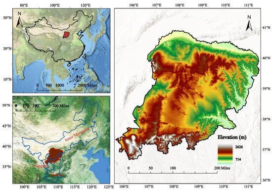
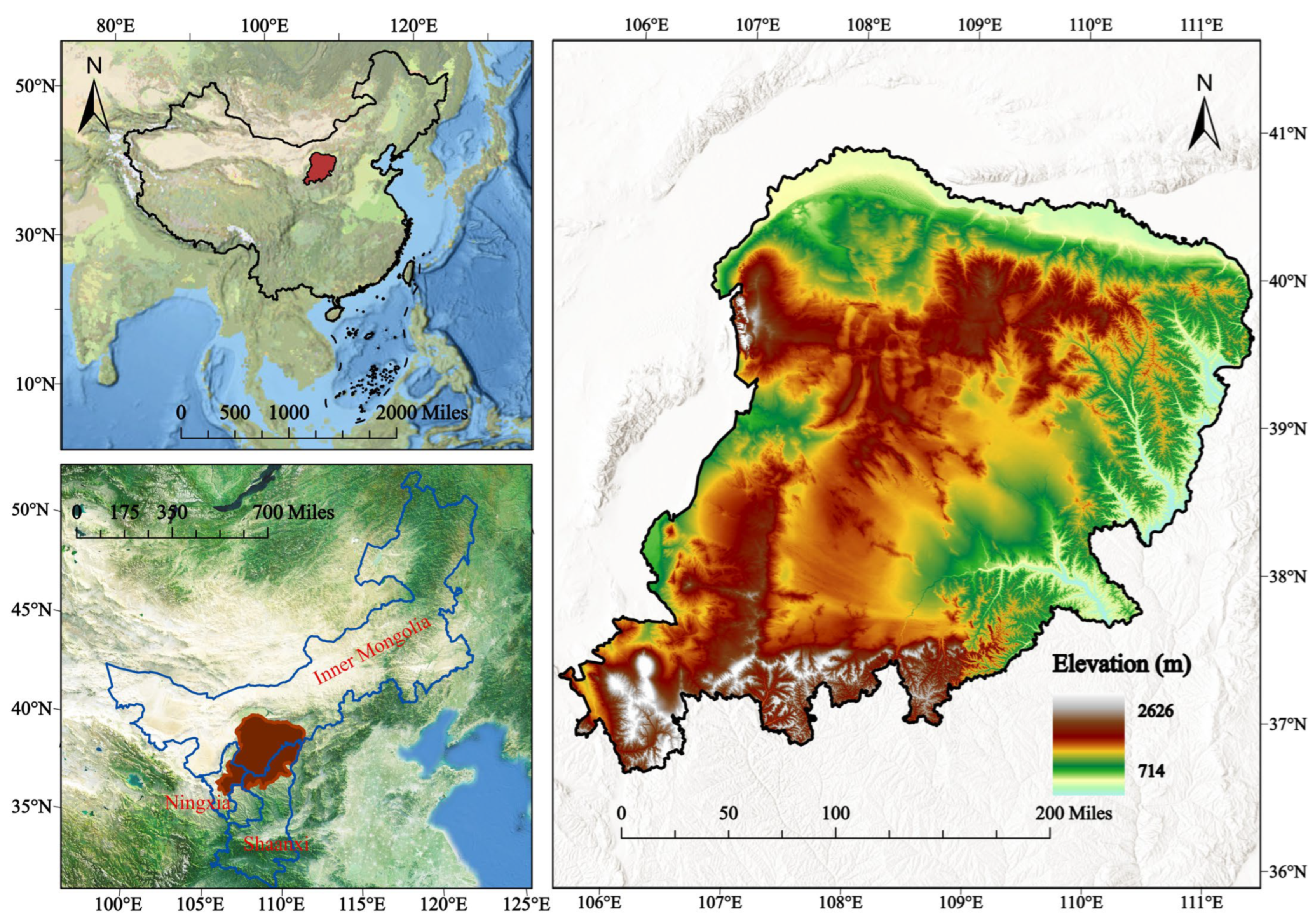
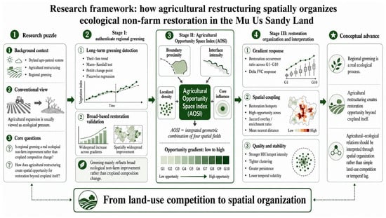
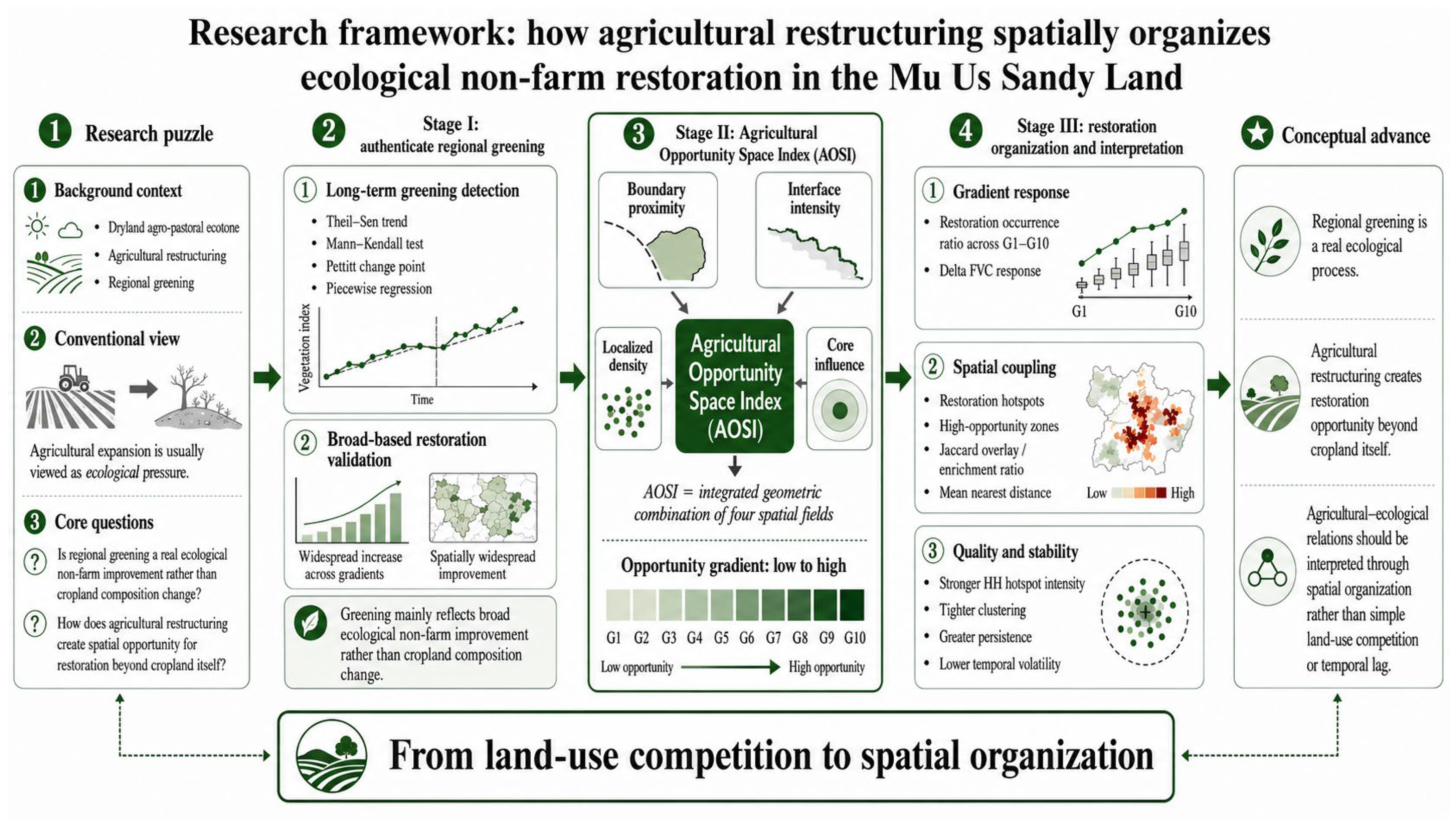
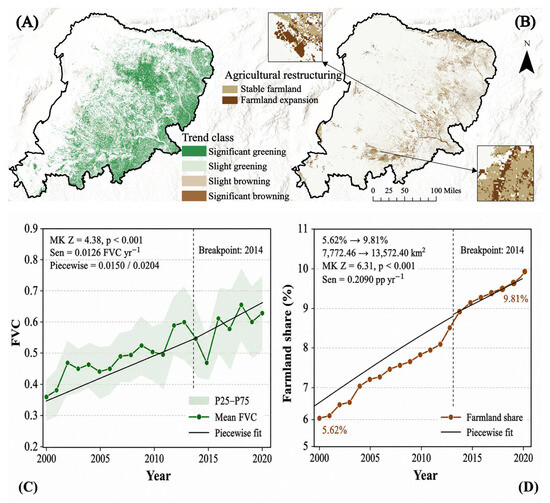
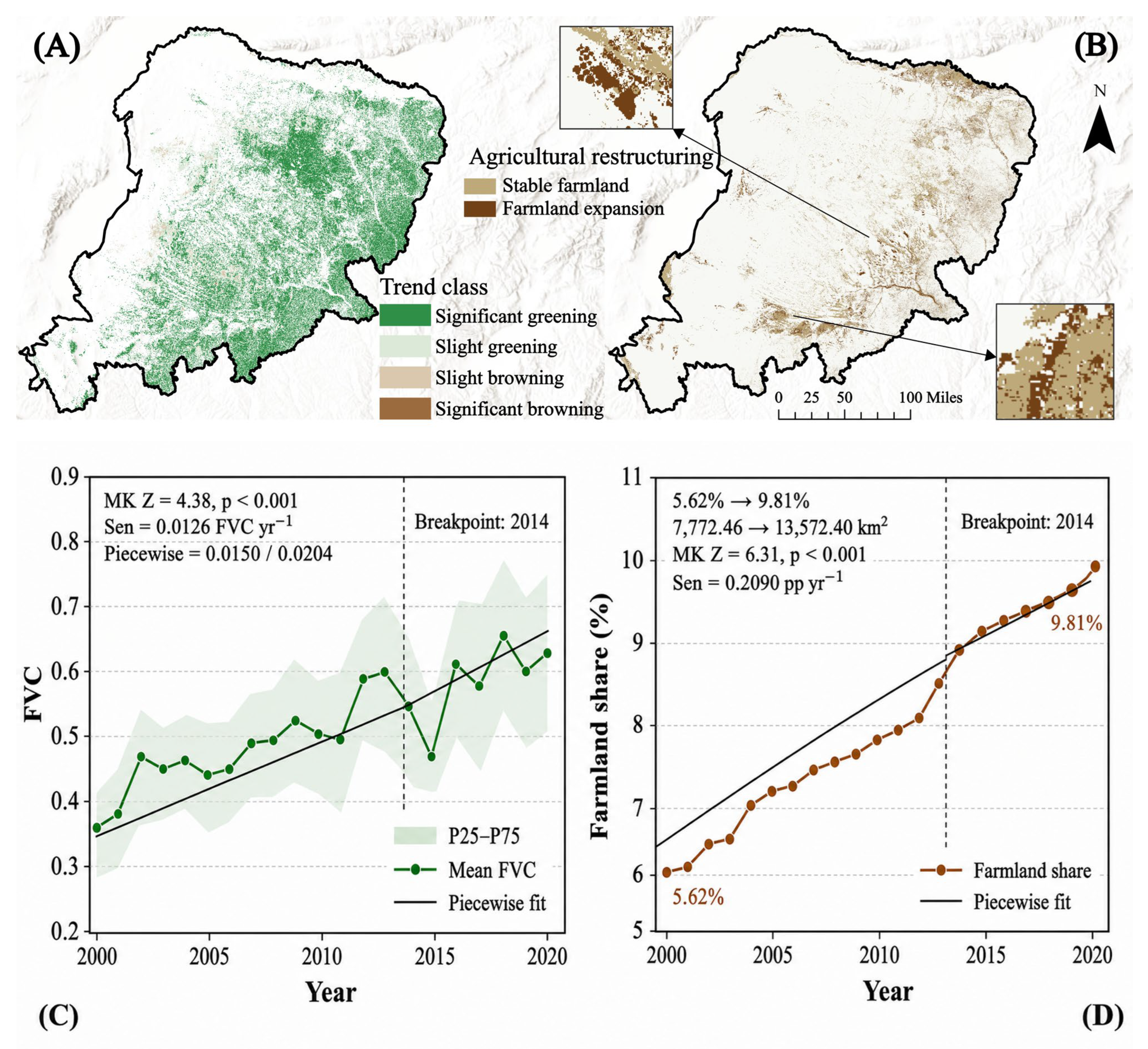
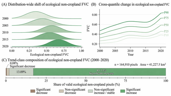
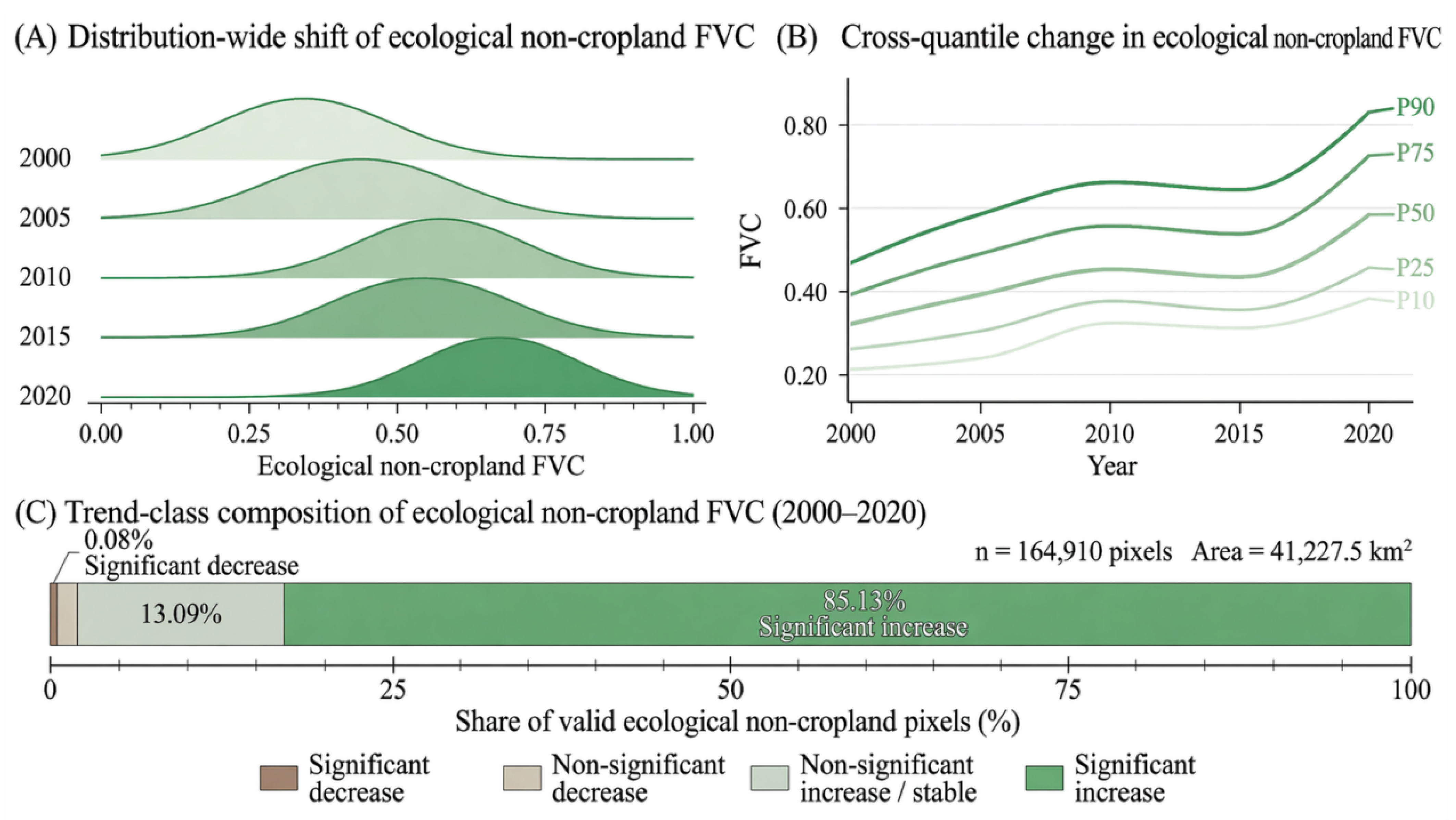
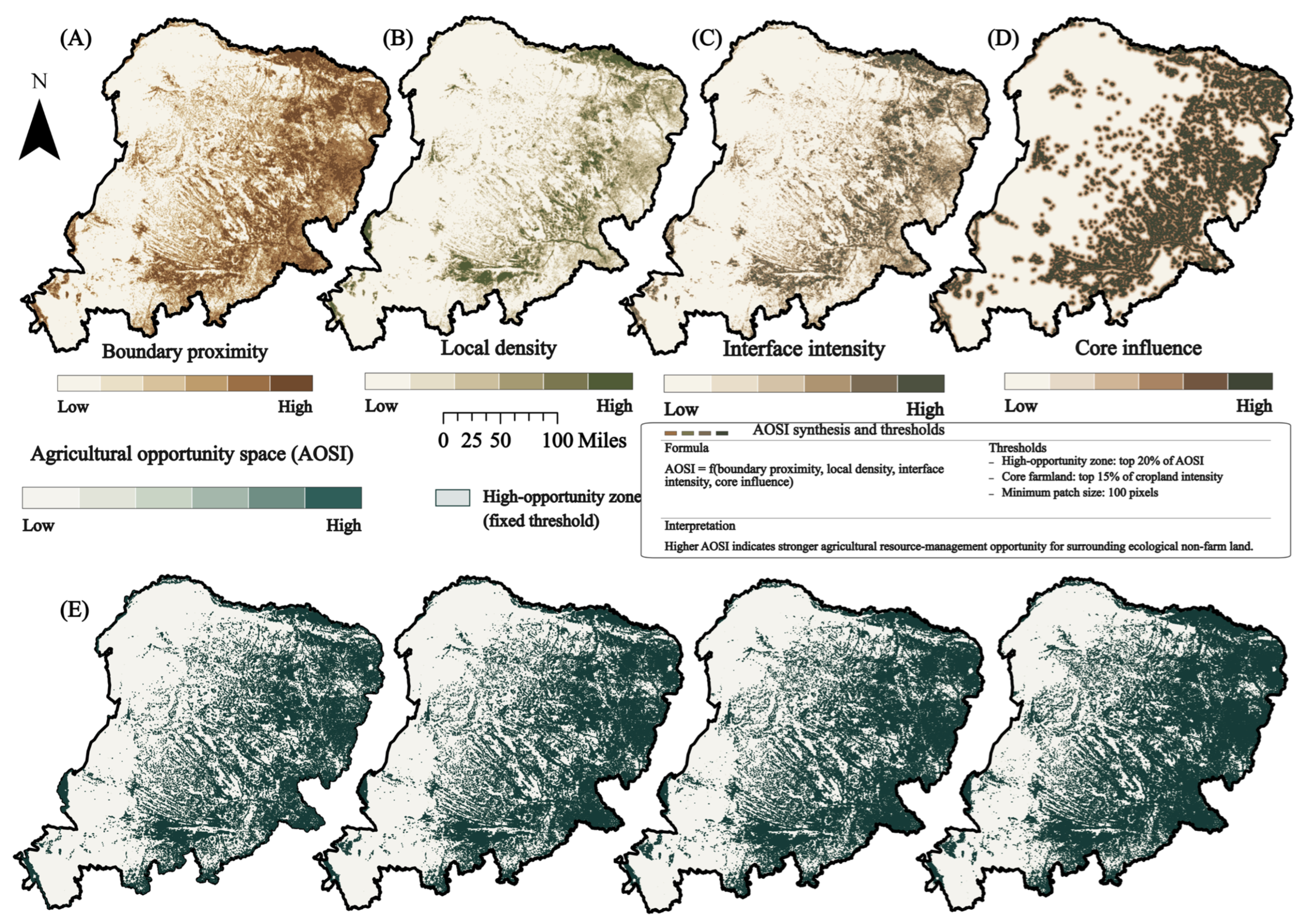
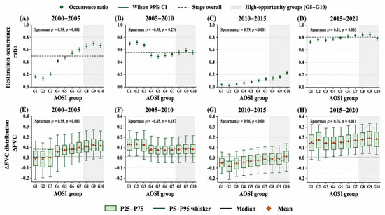
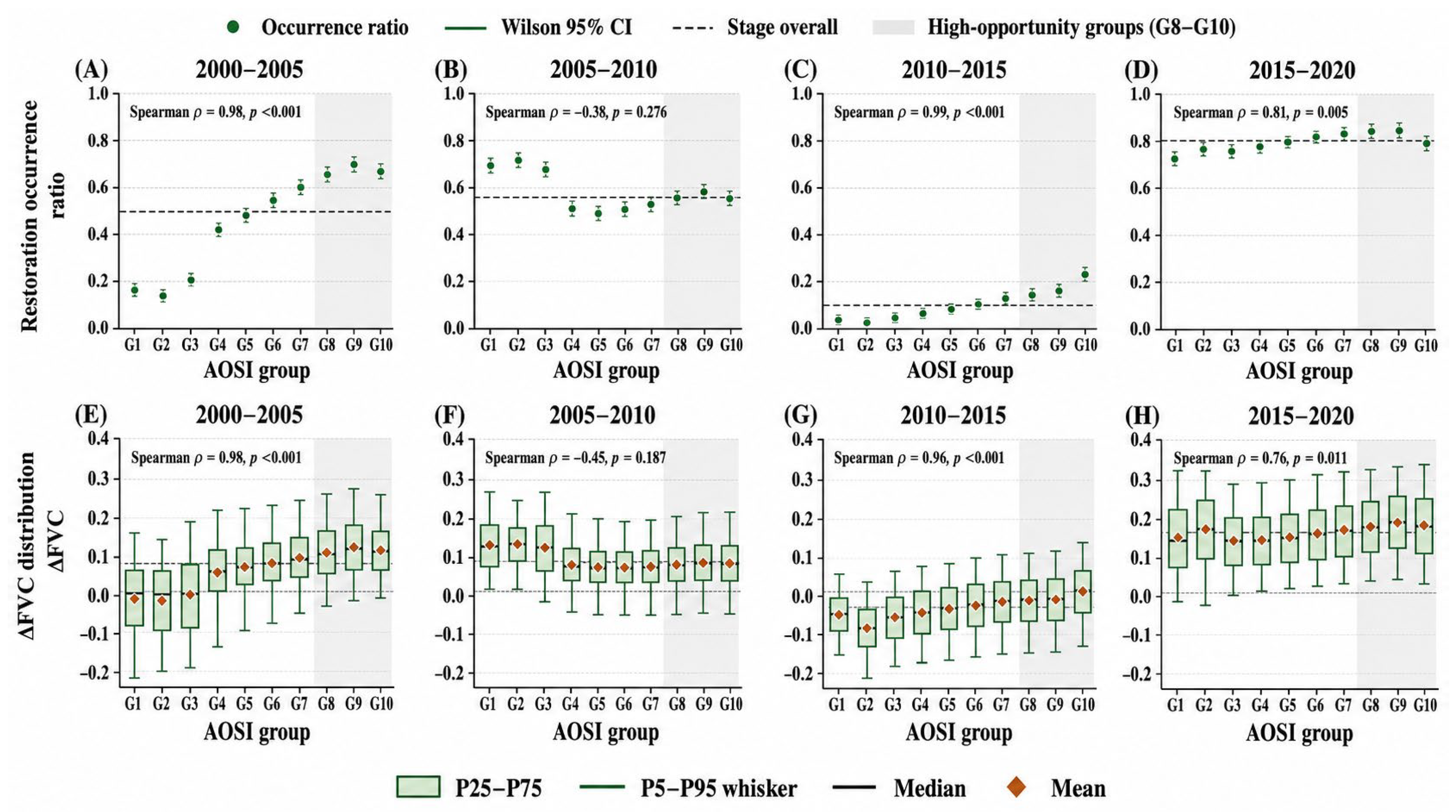
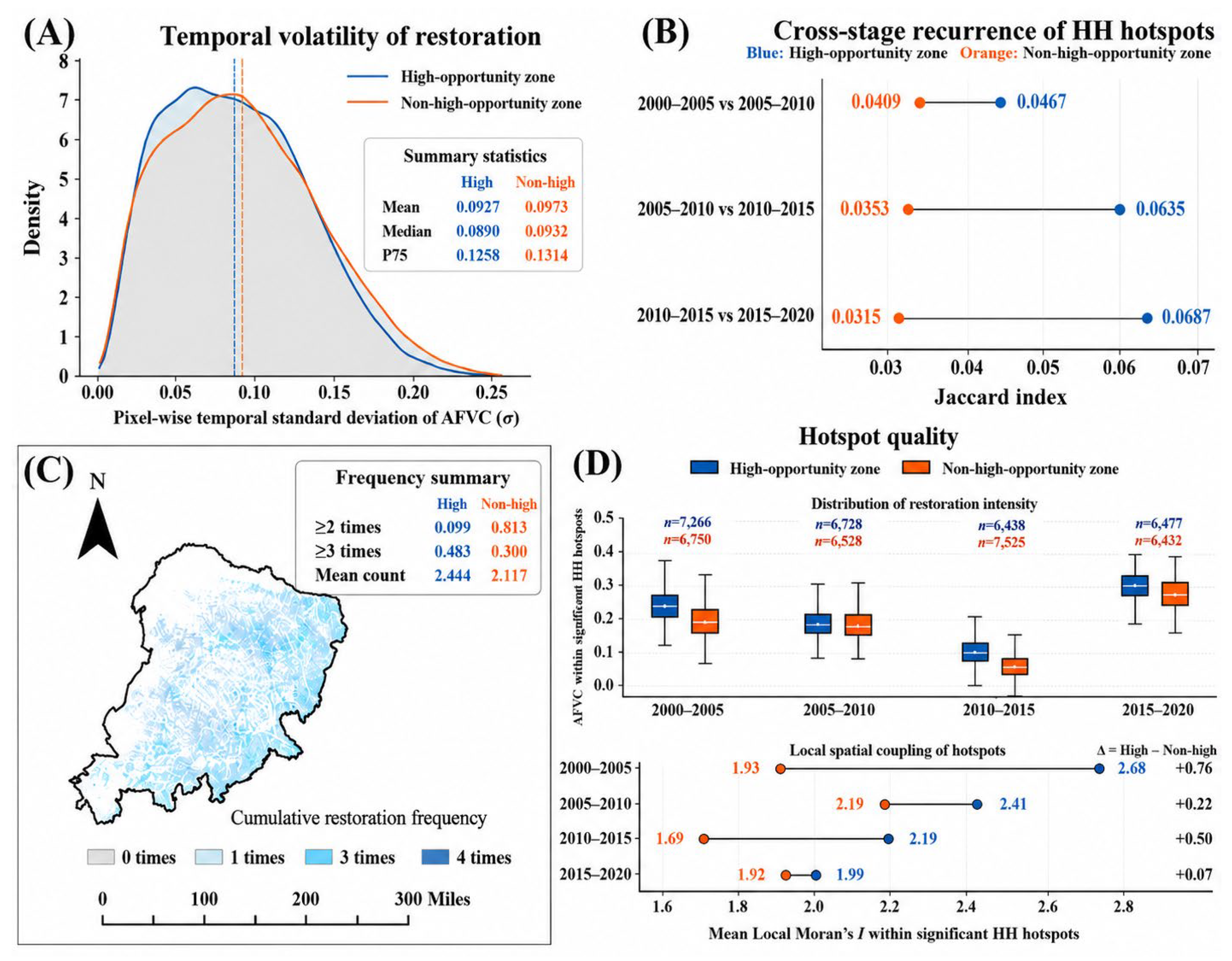

Disclaimer/Publisher’s Note: The statements, opinions and data contained in all publications are solely those of the individual author(s) and contributor(s) and not of MDPI and/or the editor(s). MDPI and/or the editor(s) disclaim responsibility for any injury to people or property resulting from any ideas, methods, instructions or products referred to in the content. |
© 2026 by the authors. Licensee MDPI, Basel, Switzerland. This article is an open access article distributed under the terms and conditions of the Creative Commons Attribution (CC BY) license.