Gated Spiking Attention Transformer for Hyperspectral Image Classification

Highlights

What are the main findings?

• Ultra-lightweight and energy-efficient spiking Transformer architectures become feasibleb for high-accuracy hyperspectral image classification on resource-constrained edge platforms.
• Reinterpreting attention as a learnable binary gate provides a new design paradigm for building event-driven vision models with extreme parameter and energy efficiency.

What are the implications of the main findings?

• Ultra-lightweight and energy-efficient spiking Transformer architectures become feasible for high-accuracy hyperspectral image classification on resource-constrained edge platforms.
• Reinterpreting attention as a learnable binary gate provides a new design paradigm for building event-driven vision models with extreme parameter and energy efficiency.

Abstract

Deploying deep learning models for hyperspectral image classification (HSIC) on resource-constrained edge or non-orbit platforms is challenging due to high energy consumption and computational cost. To address this, this paper proposes a lightweight spike-driven Vision Transformer, termed ‘GS-SpikeFormer’, leveraging energy-efficient spiking neural networks (SNNs). Our work makes three key contributions. First, we introduce a Gated Spiking Attention (GSA) mechanism that replaces costly matrix multiplication with binary event-driven feature gating using only logical AND operations. Second, we incorporate groupwise convolution into both self-attention and feedforward modules, reducing trainable parameters to just $0.35$ M while preserving local spectral-spatial feature extraction. Third, extensive experiments on four benchmark hyperspectral datasets under limited training sample show that GS-SpikeFormer achieves competitive results with only 4 time steps (e.g., $97.54\%$ on Indian Pines, $98.62\%$ on Pavia University, $98.89\%$ on Salinas, and $98.39\%$ on Houston2013). Compared to prior SNN-based HSIC methods, our model achieves superior parameter and energy efficiency.

1. Introduction

Hyperspectral image classification (HSIC) aims to assign pixel-wise labels to ground objects by using data captured through hundreds of consecutive spectral bands. The rich spectral-spatial information in hyperspectral imagery (HSI) [1] enables a wide range of applications, including environmental monitoring [2], agricultural management [3], urban planning [4], national defense [5], etc. However, the high-dimensional, complex nonlinear structures and limited availability of labeled samples make HSIC a challenging task.

Recent advances in deep learning have led to remarkable progress in HSIC. Convolutional neural networks (CNNs) are capable of effectively extracting local spectral-spatial features, but are constrained by their limited receptive field and high parameter quantities. In cases where the training data is scarce, this often leads to overfitting [6]. Vision Transformers (ViTs) capture long-range dependencies through self-attention, yet they lack inductive biases for local feature extraction and introduce prohibitive computational costs, particularly for high-dimensional HSI data [7,8]. Hybrid CNN-Transformer models, such as GSC-ViT [9] and DBCTNet [10], have shown balanced efficiency and performance, but they still fall within the domain of artificial neural networks (ANNs) and inherit the high energy consumption associated with dense floating-point operations.

Spiking neural networks (SNNs) offer a promising alternative due to their event-driven, binary spike-based computation, achieving ultra-low power inference and biological plausibility [11,12,13]. Unlike ANNs that rely on energy-intensive multiplication accumulation (MAC) operations, SNNs accumulate spikes only when events occur, making them ideally suitable for deployment on resource-constrained edge devices. This inherent efficiency has spurred interest in integrating the representational capabilities of Transformers into the SNN paradigm.

In the context of HSIC, several SNN-based methods have been developed. SNN-SSEM [12] constructed a conventional SNN with depthwise separable convolutions, but it requires a large number of time steps (e.g., T = 30) to achieve competitive accuracy. AFSA [14] introduced a spike self-attention module with adaptive refocusing, but its attention mechanism is not entirely driven by spikes and still relies on careful tuning. Neither of these methods fully exploited the potential of Transformer-style global modeling. Meanwhile, outside the field of remote sensing, SpikingResformer [15] recently demonstrated remarkable performance in large-scale image classification by proposing Dual Spike Self-Attention (DSSA) and a ResNet-inspired multi-stage architecture. However, applying SpikingResformer directly to HSIC reveals critical limitations. First, spatial resolution mismatch: SpikingResformer’s multi-stage strided convolutions and max-pooling progressively downsample feature maps from $224\times 224$ to $7\times 7$. On small HSI patches (e.g., $11\times 11$), this collapses spatial dimensions to $1\times 1$ after only a few stages, destroying the spatial structure needed for self-attention and causing severe spatial feature loss before any global dependency can be captured. Second, architectural over-parameterization: the multi-stage design with large kernel convolutions (e.g., $7\times 7$) and high-dimensional embeddings (up to 1024 channels), optimized for large-scale RGB images, becomes redundant on small HSI patches with limited samples, causing overfitting and wasted computation without accuracy gains. Third, spectral-spatial decoupling: SpikingResformer’s patch-splitting strategy treats spatial neighbors independently, ignoring the strong spectral continuity and local spatial correlations of HSI data. This exacerbates information loss on small patches, highlighting the need for a lightweight, single-stage architecture tailored to HSI’s unique spectral-spatial structure.

To address these challenges, a novel spike-driven Vision Transformer, termed ‘GS-SpikeFormer’, is proposed. It fundamentally reinterprets attention as a learnable binary gating mechanism. The core of it lies the Gated Spiking Attention (GSA) module, which replaces weighted summation with event-driven hard feature selection. By using convolution kernels to implicitly capture global spatial relationships and generating binary masks through logical AND operations, GSA achieves global context modeling in a fully spike-compatible manner. To further reduce the parameter overhead while preserving the modeling capacity, groupwise convolution is integrated into the self-attention and feedforward modules. This architecture synergistically combines GSA with a front-end Spectral Calibration (SC) module for adaptive spectral dimension processing and a Groupwise Spiking Feedforward Network (GWSFFN) for spectral-spatial feature refinement. This unified design explicitly addresses the dual challenges of high dimensions and limited training samples in HSIC.

Beyond classification, deep learning has also proven versatile in other HSI tasks [16], including semi-supervised anomaly detection with generative adversarial networks [17], unsupervised anomaly detection with memory networks [18,19], self-supervised anomaly detection with blind-spot networks [20,21]. These advances highlight the broad potential of deep learning in HSI analysis and motivate our exploration of SNN-based classification architectures.

To summarize, the main contributions of our work are threefold:

• Gated Spiking Attention (GSA). A novel spike-compatible self-attention mechanism that treats attention as a binary gating process. By employing a learnable convolution kernel to implicitly learn global spatial relationships and applying it as a hard, event-driven filter, GSA only uses logical AND operations to perform global feature selection. This design eliminates multiplications, retains full spike-driven computations, and achieves interpretable binary attention maps.
• Groupwise Convolution Integration. To overcome the typical parameter explosion problem in dense projections, groupwise convolution is simultaneously introduced into the GSA module and the feedforward network (FFN) module. This drastically reduces the number of trainable parameters (only $0.35$ M), while retaining the ability to jointly extract local spectral-spatial features and long-range dependencies, making the model exceptionally lightweight and suitable for resource-constrained edge deployment.
• Unified Spike-Driven Framework for HSIC. GS-SpikeFormer is the first fully spike-driven ViT specifically tailored for HSIC. By harmoniously integrating GSA, SC, and GWSFFN, this model achieves state-of-the-art accuracy with minimal temporal overhead: with only 4 time steps, it attains OAs of $97.54\%$ on Indian Pines, $98.62\%$ on Pavia University, $98.89\%$ on Salinas, and $98.39\%$ on Houston2013, significantly outperforming existing methods based on SNN and Transformer. End-to-end binary spike activation ensures unparalleled energy efficiency.

The remainder of this paper is organized as follows: Section 2 details the GS-SpikeFormer architecture as well as the key components. Section 3 describes experimental setup and hyperparameters analysis. Section 4 compares the proposed method with SNN-based methods. Section 5 provides comprehensive comparisons with state-of-the-art HSIC models. Section 6 discusses the experimental results, covering the advantages and limitations of our work, as well as the future research directions. Finally, Section 7 concludes the paper with future directions.

2. Methodology

In this section, we present GS-SpikeFormer, a fully spike-driven Vision Transformer specifically designed for HSIC. First, an overview of the overall architecture is provided, followed by detailed descriptions of its core components: the underlying spiking neuron model, Gated Spiking Attention (GSA), groupwise convolution integration, front-end processing modules, and classification head. The focus is on explaining how GSA reinterprets attention as a binary gating process to achieve global modeling while maintaining strictly spike-driven computation.

2.1. Overall Architecture

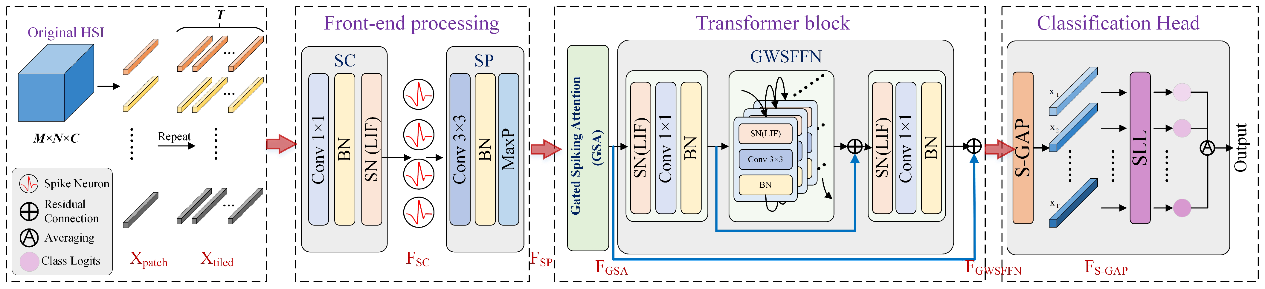
Figure 1 illustrates the overall pipeline of GS-SpikeFormer. Given an input hyperspectral data patch ${\mathbf{X}}_{\mathrm{patch}}\in {\mathbb{R}}^{H\times W\times C}$ (where H, W, and C denote height, width, and spectral bands), the model processes it through three sequential stages: front-end processing, a spike-driven Transformer block, and a classification head. Every layer, except max-pooling and temporal-averaging, operates entirely with binary spike activations and event-driven computations, ensuring end-to-end energy efficiency.

• Front-end processing adaptively reduces spectral dimensionality and extracts local spectral-spatial features while converting the original input into spike-compatible representations. It consists of a Spectral Calibration (SC) module ($1\times 1$$\mathrm{Conv}$ + $\mathrm{BN}$ + spiking neuron activation ($\mathrm{SN}$)) and a Spatial Calibration (SP) module ($3\times 3$$\mathrm{Conv}$ + $\mathrm{BN}$ + $\mathrm{SN}$ + Max-Pooling).
• Spiking-driven Transformer block is the core of the model, consisting of a Gated Spiking Attention (GSA) module and a Groupwise Spiking Feedforward Network (GWSFFN). Both of these modules are fully spike-driven and leverage groupwise convolution to reduce parameters while preserving representational capacity.
• Classification head aggregates global spatial information via spike-based global average pooling and maps it to class logits through a spiking linear layer. The final prediction is obtained by averaging the output spikes over T time steps for stability.

Figure 1. Overall architecture of GS-SpikeFormer for HSIC. All intermediate representations are binary spike tensors, and all operations (except pooling and temporal averaging) are spike-driven.

Figure 1. Overall architecture of GS-SpikeFormer for HSIC. All intermediate representations are binary spike tensors, and all operations (except pooling and temporal averaging) are spike-driven.

Table 1. Architectural details of the proposed GS-SpikeFormer. ‘SC’ denotes Spectral Calibration module, ‘SP’ denotes Spatial Calibration module, ‘MaxP’ denotes Max-Pooling, ‘GSA’ is Gated Spiking Attention, ‘GWSFFN’ is Groupwise Spiking Feedforward Network, ‘S-GAP’ denotes Spike-based Global Average Pooling, and ‘SSL’ denotes Spiking Linear Layer. The size of the input patch varies according to the dataset.

Stage	Layer	Input Size	Output Size	Kernel Size	Stride	Groups	Spike-Driven
Front-end	SC	$T\times C\times H\times W$	$T\times 256\times H\times W$	$1\times 1$	1	1	Yes (LIF)
	SP	$T\times 256\times H\times W$	$T\times 64\times H\times W$	$3\times 3$	1	1	Yes (LIF)
	MaxP	$T\times 64\times H\times W$	$T\times 64\times (H-1)\times (W-1)$	$2\times 2$	1	–	No
Transformer	GSA	$T\times 64\times (H-1)\times (W-1)$	$T\times 64\times (H-1)\times (W-1)$	–	–	16/32 1	Yes (LIF)
	GWSFFN	$T\times 64\times (H-1)\times (W-1)$	$T\times 64\times (H-1)\times (W-1)$	$3\times 3$	1	64 2	Yes (LIF)
Classification	S-GAP	$T\times 64\times (H-1)\times (W-1)$	$T\times 64\times 1\times 1$	–	–	–	No
	SLL	$T\times 64$	$N_{\mathrm{class}}\times 1$	Linear	–	–	Yes (LIF)

¹ Group numbers are dataset-adaptive: 16 for Indian Pines (IP) and Pavia University (PU); 32 for Salinas (SA) and Houston2013 (HU). ² Group size = 64 channels per group.

details the layer-wise configurations, including tensor shapes, kernel sizes, group settings, and spike-driven compatibility.

2.2. Spiking Neuron Model

All spiking computations in GS-SpikeFormer are based on the Leaky Integrate-and-Fire (LIF) neuron, which offers a favorable balance between biological plausibility and computational efficiency. Its discrete-time dynamics are described as follows:

$$v_i\left[t\right]=u_i\left[t\right]+{\displaystyle \frac{1}{\tau }}\left(I_i\left[t\right]-(u_i\left[t\right]-u_{\mathrm{rest}})\right),$$

(1)

$$I_i\left[t\right]={\sum }_j{w}_{i,j}{s}_j\left[t\right],$$

(2)

$$s_i\left[t\right]=\Theta (v_i\left[t\right]-u_{\mathrm{th}}),$$

(3)

$$u_i[t+1]=s_i\left[t\right]u_{\mathrm{rest}}+(1-s_i\left[t\right])v_i\left[t\right].$$

(4)

Here, $u_i\left[t\right]$ and $v_i\left[t\right]$ denote the membrane potential before and after charging. $\tau$ is the membrane time constant controlling leakage rate, a larger $\tau$ means slower leakage, allowing the neuron to remember inputs for longer. $I_i\left[t\right]$ is the input current at time t, computed as the weighted sum of incoming spikes $s_j\left[t\right]$ from presynaptic neurons (Formula (2)), $w_{i,j}$ are synaptic weights, and $u_{\mathrm{rest}}$ is the resting potential. As illustrated in Formula (1), the membrane potential update of a neuron is based on the input current and its previous state. Furthermore, Formula (3) indicates that a spike is generated if the membrane potential $v_i\left[t\right]$ exceeds a predefined firing threshold $u_{\mathrm{th}}$, where $\Theta (·)$ is the Heaviside step function. After firing a spike, the membrane potential is reset by using Formula (4), which means, if the incoming spikes $s_i\left[t\right]=1$, the membrane potential $u_i[t+1]$ is reset to $u_{\mathrm{rest}}$; otherwise, it retains its current value.

For brevity, we denote a spiking neuron layer as $\mathbf{S}=\mathrm{SN}\left(\mathbf{I}\right)$, where $\mathbf{I}\in {\mathbb{R}}^{T\times n}$ is the input current over T time steps for n neurons, and $\mathbf{S}\in {\{0,1\}}^{T\times n}$ is the output spike tensor.

2.3. Gated Spiking Attention (GSA)

The core innovation of GS-SpikeFormer is the Gated Spiking Attention mechanism, which fundamentally reinterprets self-attention as a learnable binary gating process. Unlike standard attention that computes weighted sums via floating-point matrix multiplications and $\mathrm{Softmax}$, GSA generates a binary mask that selectively gates the flow of spike features. This design is fully spike-driven, uses only logical AND and addition operations, and eliminates all multiplications.

2.3.1. Motivation and Design Principle

In conventional ViTs, attention maps are calculated as $\mathrm{Softmax}({\mathbf{QK}}^{\top }/\sqrt{d})\mathbf{V}$, which involves expensive matrix multiplication and $\mathrm{Softmax}$ normalization. All these operations are incompatible with the sparse and event-driven nature of SNNs. Moreover, the resulting attention weights are continuous and often redundant.

In a spike-based system, information can be gated through binary masks: a feature either passes (if the corresponding gate is 1) or is blocked (if the corresponding gate is 0). This binary gating aligns naturally with the all-or-nothing spike communication in SNNs. Therefore, the continuous attention weights with a learnable binary mask indicate which spatial positions should interact with each other. The mask is generated by a lightweight convolution kernel, which implicitly learns global spatial relationships and avoid explicit pairwise similarity calculations.

2.3.2. Formulation of GSA

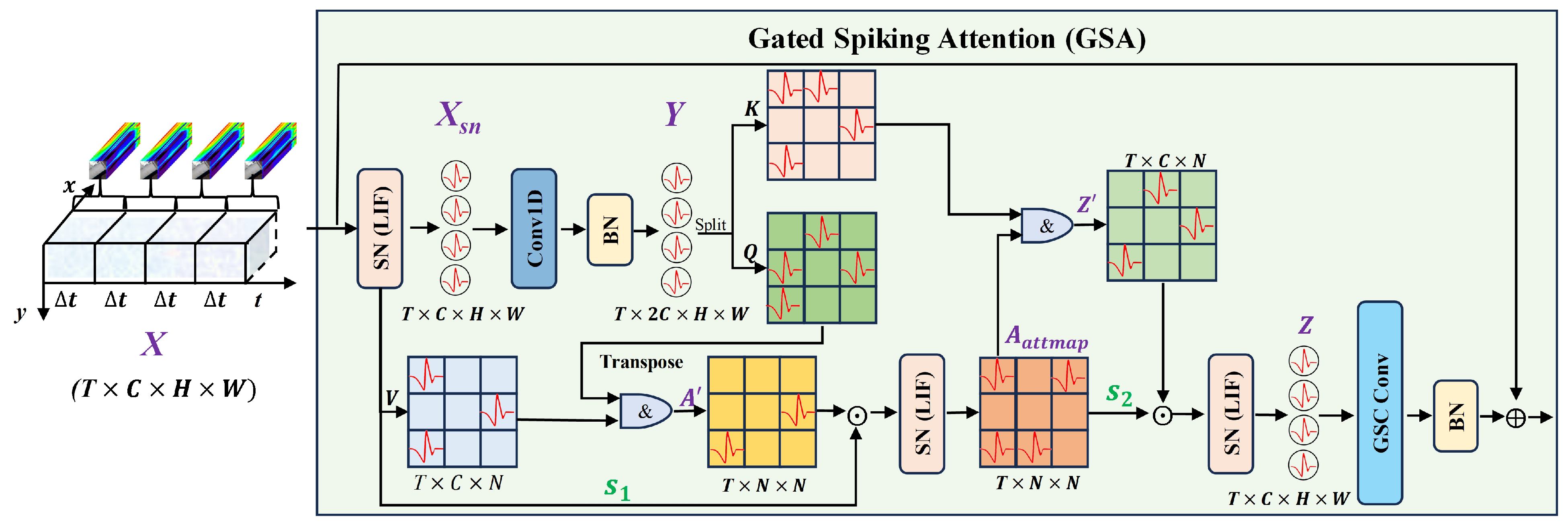
Let $\mathbf{X}\in {\{0,1\}}^{T\times C\times H\times W}$ be the input spike tensor of the GSA module (after the front-end processing). The calculation is carried out in several steps, and all steps maintain the binary spike representation (as shown in Figure 2).

• Preliminary activation. The input spike tensor $\mathbf{X}$ first passes through a spiking neuron layer ($\mathrm{SN}$) to ensure binary activations:

  $${\mathbf{X}}_{\mathrm{sn}}=\mathrm{SN}\left(\mathbf{X}\right).$$

  (5)
• Query and Key generation. Instead of projecting the ${\mathbf{X}}_{\mathrm{sn}}$ onto three separate matrices, a single spike-compatible convolution with a kernel size of $p\times p$ (here $p=1$) is applied, followed by batch normalization ($\mathrm{BN}$):

  $$\mathbf{Y}=\mathrm{BN}\left({\mathrm{Conv}}_{2C,C}^{(1\times 1)}\left({\mathbf{X}}_{\mathrm{sn}}\right)\right)\in {\{0,1\}}^{T\times 2C\times H\times W}.$$

  (6)
  Then, along the channel dimension, $\mathbf{Y}$ is split into two tensors $\mathbf{Q}$ and $\mathbf{K}$, which have the same size as $T\times C\times H\times W$ and are served as Query and Key respectively. Notably, the Value $\mathbf{V}$ is directly taken from the input ${\mathbf{X}}_{\mathrm{sn}}$ (after reshaping) to reduce parameters and preserve sparsity.
  Furthermore, the Query, Key, and Value tensors can also be split into multiple heads. Specifically, the channel dimension C is divided into $n\_h$ groups, and the dimension of each head group is $d_h=C/n\_h$. Each head independently performs spike-based attention, allowing the model to focus on different feature subspaces. The outputs of all heads are concatenated and linearly projected back to the original dimension. This multi-head design enables the model to capture diverse spatial dependencies, which is particularly beneficial for hyperspectral data that may exhibit different correlations in different spectral bands.
• Binary attention map. The attention map is obtained via a spike-based matrix multiplication between the transposed $\mathbf{Q}$ and the reshaped $\mathbf{V}$. Since all the operands are binary, the multiplication becomes a logical AND operation, and the sum over the feature dimensions is simply the count of coincidence spikes. Specifically, $\mathbf{Q}$ and $\mathbf{V}$ are shaped as $(T,C,N)$ with $N=H\times W$ and the calculation is as follows:

  $${\mathbf{A}}^{\prime }={\mathbf{Q}}^{\top }\mathbf{V}.$$

  (7)
  Although expressed as a matrix product, Formula (7) reduces to logical AND followed by integer addition because both $\mathbf{Q}$ and $\mathbf{V}$ are binary spike tensors, effectively counting coincident spikes. This multiplication-free computation is naturally suited for event-driven hardware and produces an integer counting matrix ${\mathbf{A}}^{\prime }\in {\mathbb{R}}^{T\times N\times N}$.
  To normalize these counts to a valid range while maintaining spike compatibility, a fixed scaling factor $s_1$ is applied according to the standard practice in the Transformer architecture:

  $$s_1={\displaystyle \frac{1}{\sqrt{d_h}}}.$$

  (8)
  Here $d_h$ represents the embedding dimension for each head. This constant scaling avoids potential training instability caused by the dynamically varying firing rate. The scaled mapping $\mathbf{A}={\mathbf{A}}^{\prime }\odot s_1$ is then passed through a spiking neuron layer to obtain a binary attention map:

  $${\mathbf{A}}_{\mathrm{attmap}}=\mathrm{SN}\left(\mathbf{A}\right)\in {\{0,1\}}^{T\times N\times N}.$$

  (9)
  Each nonzero entry in ${\mathbf{A}}_{\mathrm{attmap}}$ indicates that the corresponding pair of spatial locations should interact.
• Feature gating. The output features are computed by applying the binary attention map ${\mathbf{A}}_{\mathrm{attmap}}$ to the Key (or the second part of the projection) via another spike-based matrix multiplication:

  $${\mathbf{Z}}^{\prime }=\mathbf{K}{\mathbf{A}}_{\mathrm{attmap}}.$$

  (10)
  Similarly, Formula (10) involves no floating-point multiplications. The binary attention map ${\mathbf{A}}_{\mathrm{attmap}}$ serves as a gating mask, accumulating key features at 1-entries and blocking at 0-entries, implemented purely by event-driven addition without any multiply-accumulate (MAC) operations.
  ${\mathbf{Z}}^{\prime }$ is then scaled by a second factor $s_2$,

  $$s_2={\displaystyle \frac{1}{\sqrt{N}}},$$

  (11)

  where $N=H\times W$ represents the number of spatial positions. This scaling factor reflects the design in [15] and ensures stable training across different input resolutions. The scaled results are passed through a spiking neuron layer:

  $$\mathbf{Z}=\mathrm{SN}({\mathbf{Z}}^{\prime }\odot s_2)\in {\{0,1\}}^{T\times C\times N}.$$

  (12)
  Finally, $\mathbf{Z}$ is reshaped back to $(T,C,H,W)$.
• Groupwise output projection. To incorporate information across channels while maintaining spike-driven calculations, we employed a groupwise separable convolution (GSC) (refer to Section 2.4.1 for details). To ensure divisibility, the effective number of groups is automatically set to the greatest common divisor of the channel dimension C and the intended number of groups (e.g., 16 or 32). A residual connection adds the original input $\mathbf{X}$:

  $${\mathbf{F}}_{\mathrm{GSA}}=\mathrm{BN}\left({\mathrm{Conv}}_{C,C}^{\mathrm{GSC}}\left(\mathbf{Z}\right)\right)+\mathbf{X}.$$

  (13)

In order to better understand the calculation process of GSA, we provide a pseudo-code description in Algorithm 1.

Algorithm 1 Pseudo-code of the calculation process of GSA.

Require:  Spike tensor $\mathbf{X}\in {\{0,1\}}^{T\times C\times H\times W}$, number of heads $\mathrm{n}\_\mathrm{h}$, groups g Ensure:  Output spike tensor ${\mathbf{F}}_{\mathrm{GSA}}\in {\{0,1\}}^{T\times C\times H\times W}$ 1: ${\mathbf{X}}_{\mathrm{sn}}\leftarrow \mathrm{SN}\left(\mathbf{X}\right)$                     ▹ Ensure binary activation 2: $\mathbf{Y}\leftarrow \mathrm{BN}\left({\mathrm{Conv}}_{2C,C}^{(1\times 1)}\left({\mathbf{X}}_{\mathrm{sn}}\right)\right)$          ▹ Spike-compatible $1\times 1$ convolution 3: Split $\mathbf{Y}$ along channels into $\mathbf{Q},\mathbf{K}\in {\{0,1\}}^{T\times C\times H\times W}$ 4: $\mathbf{V}\leftarrow {\mathbf{X}}_{\mathrm{sn}}$                      ▹ Use original spikes as Value 5: Reshape $\mathbf{Q},\mathbf{K},\mathbf{V}$ to $(T,n\_h,d_h,N)$, where $N=H\times W$, $d_h=C/n\_h$ 6: for$h=1$ to $\mathrm{n}\_\mathrm{h}$ do 7:     ${\mathbf{Q}}_h,{\mathbf{K}}_h,{\mathbf{V}}_h\leftarrow$ slices of $\mathbf{Q},\mathbf{K},\mathbf{V}$ for head h           ▹ Shape: $(T,d_h,N)$ 8:     ${\mathbf{A}}_h^{\prime }\leftarrow {\mathbf{Q}}_h^{\mathsf{T}}{\mathbf{V}}_h$          ▹ Logical AND and summation; shape: $(T,N,N)$ 9:     $s_1\leftarrow 1/\sqrt{d_h}$ 10:     ${\mathbf{A}}_{\mathrm{att},h}\leftarrow \mathrm{SN}({\mathbf{A}}_h^{\prime }\odot s_1)$                ▹ Binary attention map 11:     ${\mathbf{Z}}_h^{\prime }\leftarrow {\mathbf{K}}_h{\mathbf{A}}_{\mathrm{att},h}$         ▹ Logical AND and summation; shape: $(T,d_h,N)$ 12:     $s_2\leftarrow 1/\sqrt{N}$ 13:     ${\mathbf{Z}}_h\leftarrow \mathrm{SN}({\mathbf{Z}}_h^{\prime }\odot s_2)$                    ▹ Gated features 14: end for 15: Concatenate ${\left\{{\mathbf{Z}}_h\right\}}_{h=1}^{\mathrm{n}\_\mathrm{h}}$ to ${\mathbf{Z}}_{\mathrm{cat}}\in {\{0,1\}}^{T\times C\times N}$, then reshape to $(T,C,H,W)$ as $\mathbf{Z}$ 16: ${\mathbf{Z}}_{\mathrm{proj}}\leftarrow \mathrm{BN}\left({\mathrm{GroupwiseSeparableConv}}_{C,C}(\mathbf{Z},g)\right)$      ▹ GSC output projection 17: ${\mathbf{F}}_{\mathrm{GSA}}\leftarrow {\mathbf{Z}}_{\mathrm{proj}}+\mathbf{X}$           ▹ Residual connection return ${\mathbf{F}}_{\mathrm{GSA}}$

2.3.3. Why GSA Works as Attention

The binary attention map A_attmap generated by GSA functions analogously to standard attention weights, indicating which spatial positions may exchange information, except that the weights are binarized through a spiking nonlinearity. The map acts as a hard gate: a feature is accumulated only when both the corresponding Query and Key positions emit a spike, implementing an event-driven, multiplication-free gating mechanism.

Although A_attmap is binary, the expressive power of the attention is preserved through three complementary designs: First, learnable convolutional projections encode rich spatial context before binarization, and the spiking threshold serves as a decision boundary that retains only statistically salient spatial correlations. Second, multiple parallel heads specialize in different spatial patterns, collectively capturing diverse dependencies. Third, after gating, a groupwise separable output projection mixes information across channels, restoring representational capacity. In this way, the collective behavior across heads and channels enables GSA to approximate soft attention effectively while staying fully spike-compatible. This reformulation of attention as a learnable binary gating process, rather than a weighted sum, aligns naturally with the event-driven philosophy of SNNs.

2.4. Groupwise Convolution Integration

To achieve extreme parameter efficiency without sacrificing representational capacity, GS-SpikeFormer incorporates groupwise convolutions in two critical places: the output projection of GSA and the feedforward network.

2.4.1. Groupwise GSA Revisited

The grouping convolution strategy employed by GSA on the output projection is directly inspired by the Groupwise Separable Convolution (GSC) proposed in GSC-ViT [9]. GSC factorizes the standard convolution into two sequential operations: Grouped Pointwise Convolution (GPWC) which combines the information within the channel groups, and then Grouped Convolution (GC) which extracts the spatial features within the same groups. This decomposition reduces the parameter count by approximately a factor equal to the number of groups, while retaining the ability to learn rich representations.

Specifically, after computing the spike-based attention output $\mathbf{Z}$ (Formula (12)), we apply grouped $1\times 1$ convolution to project the features back to the original channel dimension. This grouped projection can be regarded as a form of GPWC: it independently performs cross-channel mixing within each group, significantly reducing the parameter count compared to the standard dense projection. Moreover, a $3\times 3$ convolution is applied within the same group subsequently to extract spatial features, which can be considered as a form of GC.

The number of groups g in the output projection is a hyperparameter that balances parameter efficiency and representational capacity. For instance, when $C=64$ and $g=16$, the grouped $1\times 1$ convolution has approximately $C^2/g=256$ parameters. In contrast, the dense projection has $C^2=4096$ parameters, which is 16-fold reduction. This drastic savings enables GSA to maintain global modeling capabilities with extremely lightweight footprint.

2.4.2. Groupwise Spiking Feedforward Network (GWSFFN)

The GWSFFN module replaces the traditional multi-layer perceptron (MLP) with a more efficient design that leverages grouped convolutions for local feature refinement. Its structure is as follows:

• Channel expansion: A $1\times 1$ convolution expands the channel dimension by a factor of 4, followed by $\mathrm{BN}$ and spiking neuron activation.

  $${\mathbf{Z}}_{\mathrm{up}}=\mathrm{BN}\left({\mathrm{Conv}}_{4C,C}^{(1\times 1)}\left(\mathrm{SN}\left({\mathbf{F}}_{\mathrm{GSA}}\right)\right)\right).$$

  (14)
• Local refinement: A sequence of grouped $3\times 3$ convolutions (a group of 64 channels) with $\mathrm{BN}$ and spiking neuron activation, plus a residual connection that adds the input of this stage.

  $$\begin{array}{cc}\hfill {\mathbf{Z}}_{\mathrm{mid}}^{\left(i\right)}& =\mathrm{BN}\left({\mathrm{Conv}}_{4C,4C}^{(3\times 3)}\left(\mathrm{SN}\left({\mathbf{Z}}_{\mathrm{mid}}^{(i-1)}\right)\right)\right),\hfill \\ \hfill {\mathbf{Z}}_{\mathrm{mid}}^{\left(N_{\mathrm{conv}}\right)}& ={\mathbf{Z}}_{\mathrm{mid}}^{\left(N_{\mathrm{conv}}\right)}+{\mathbf{Z}}_{\mathrm{up}}.\hfill \end{array}$$

  (15)
  Where $i=1,\dots ,N_{\mathrm{conv}}$, $N_{\mathrm{conv}}$ is the number of convolution kernels, ${\mathbf{Z}}_{\mathrm{mid}}^{\left(0\right)}={\mathbf{Z}}_{\mathrm{up}}$.
• Channel projection: A $1\times 1$ convolution compresses the channels back to the original dimension, followed by $\mathrm{BN}$, spiking neuron activation, and another residual connection.

  $${\mathbf{F}}_{\mathrm{GWSFFN}}=\mathrm{BN}\left({\mathrm{Conv}}_{C,4C}^{(1\times 1)}\left(\mathrm{SN}\left({\mathbf{Z}}_{\mathrm{mid}}^{\left(N_{\mathrm{conv}}\right)}\right)\right)\right)+{\mathbf{F}}_{\mathrm{GSA}}.$$

  (16)

The grouped convolution in the refinement stage enables the network to capture fine spectral-spatial patterns with minimal parameters, which is crucial for hyperspectral data where local texture and spectral correlations are discriminative.

2.5. Front-End Processing and Classification Head

The front-end processing consists of two lightweight spike-compatible modules designed to handle the high dimensionality of HSI while preserving spatial details.

2.5.1. Spectral Calibration (SC)

A $1\times 1$ convolution adjusts the original spectral dimension to 256, followed by $\mathrm{BN}$ and spiking neuron activation. This operation compresses spectral redundancy and initiates spike-based computation.

$${\mathbf{F}}_{\mathrm{SC}}=\mathrm{SN}\left(\mathrm{BN}\left({\mathrm{Conv}}_{256,C}^{(1\times 1)}\left({\mathbf{X}}_{\mathrm{patch}}\right)\right)\right).$$

(17)

2.5.2. Spatial Calibration (SP)

A $3\times 3$ convolution further reduces channels from 256 to 64, extracts local spectral-spatial features, and is followed by $\mathrm{BN}$ and spiking neuron activation. To retain fine spatial boundaries, we apply stride-1 Max-Pooling:

$$\begin{array}{cc}\hfill {\mathbf{F}}_{\mathrm{SP}}& =\mathrm{SN}\left(\mathrm{BN}\left({\mathrm{Conv}}_{64,256}^{(3\times 3)}\left({\mathbf{F}}_{\mathrm{SC}}\right)\right)\right),\hfill \\ \hfill {\mathbf{F}}_{\mathrm{SP}}& =\mathrm{MaxP}\left({\mathbf{F}}_{\mathrm{SP}}\right).\hfill \end{array}$$

(18)

Unlike GSC-ViT [9] which uses strided convolutions, our stride-1 pooling preserves spatial resolution, avoids the loss of fine object boundaries, which is critical for pixel-wise classification.

2.5.3. Classification Head

In the classification stage, global average pooling is performed over spatial dimensions using integer arithmetic:

$${\mathbf{F}}_{\mathrm{S}-\mathrm{GAP}}={\displaystyle \frac{1}{HW}}\sum _{i,j}{\mathbf{F}}_{\mathrm{trans},ij},$$

(19)

where ${\mathbf{F}}_{\mathrm{trans}}$ is the output of the Transformer stage. Subsequently, a spiking linear layer (SLL) maps ${\mathbf{F}}_{\mathrm{S}-\mathrm{GAP}}$ to class logits, and the final prediction is obtained by averaging over time steps:

$$\begin{array}{cc}\hfill \mathbf{y}& ={\displaystyle \frac{1}{T}}{\displaystyle \sum _{t=1}^T}\mathrm{SLL}\left({\mathbf{F}}_{\mathrm{S}-\mathrm{GAP}}\left[t\right]\right),\hfill \\ \hfill \widehat{\mathbf{y}}& =\arg \underset{i}{\max }\left({\mathbf{y}}_i\right).\hfill \end{array}$$

(20)

This temporal averaging stabilizes the output while preserving the event-driven nature.

Finally, to better illustrate the complete classification pipeline of the GS-SpikeFormer framework, we provide a pseudo-code description in Algorithm 2.

Algorithm 2 Pseudo-code of the complete classification pipeline of the GS-SpikeFormer framework.

Require: HSI patch ${\mathbf{X}}_{\mathrm{patch}}\in {\mathbb{R}}^{H\times W\times C}$, time steps T, heads $n\_h$, groups g Ensure: Predicted class label $\widehat{\mathbf{y}}$ 1: ${\mathbf{X}}_{\mathrm{tiled}}\leftarrow \mathrm{Repeat}({\mathbf{X}}_{\mathrm{patch}},T)$                      ▹ Shape: $(T,C,H,W)$ 2: // Front-end processing 3: ${\mathbf{F}}_{\mathrm{SC}}\leftarrow \mathrm{SN}\left(\mathrm{BN}\left({\mathrm{Conv}}_{256,C}^{1\times 1}\left({\mathbf{X}}_{\mathrm{tiled}}\right)\right)\right)$ 4: ${\mathbf{F}}_{\mathrm{SP}}\leftarrow \mathrm{SN}\left(\mathrm{BN}\left({\mathrm{Conv}}_{64,256}^{3\times 3}\left({\mathbf{F}}_{\mathrm{SC}}\right)\right)\right)$ 5: ${\mathbf{F}}_{\mathrm{SP}}\leftarrow \mathrm{MaxPool}2\mathrm{D}({\mathbf{F}}_{\mathrm{SP}},\mathrm{kernel}=2,\mathrm{stride}=1)$        ▹ Shape: $(T,64,H-1,W-1)$ 6: // Transformer block 7: ${\mathbf{F}}_{\mathrm{GSA}}\leftarrow \mathrm{GSA}({\mathbf{F}}_{\mathrm{SP}},n\_h,g)$                        ▹ See Algorithm 1 8: ${\mathbf{F}}_{\mathrm{GWSFFN}}\leftarrow \mathrm{GWSFFN}\left({\mathbf{F}}_{\mathrm{GSA}}\right)$                      ▹ See details below 9: // Classification head 10: ${\mathbf{F}}_{\mathrm{S}-\mathrm{GAP}}\leftarrow {\displaystyle \frac{1}{HW}}{\sum }_{i,j}{\mathbf{F}}_{\mathrm{GWSFFN},:,,i,j}$             ▹ Global avg pool; shape: $(T,64)$ 11: $\mathbf{y}\leftarrow \mathbf{0}$ 12: for$t=1$ to T do 13:     ${\mathbf{y}}_t\leftarrow \mathrm{SN}\left(\mathrm{SLL}\left({\mathbf{F}}_{\mathrm{S}-\mathrm{GAP}}\left[t\right]\right)\right)$          ▹ Spiking linear layer; shape: $\left(N_{\mathrm{class}}\right)$ 14:     $\mathbf{y}\leftarrow \mathbf{y}+{\mathbf{y}}_t$ 15: end for 16: $\mathbf{y}\leftarrow \mathbf{y}/T$ 17: $\widehat{y}\leftarrow argmax\left(\mathbf{y}\right)$ 18: return$\widehat{y}$ Function$\mathrm{GWSFFN}\left(\mathbf{X}\right)$: 1: ${\mathbf{Z}}_{\mathrm{up}}\leftarrow \mathrm{BN}\left({\mathrm{Conv}}_{4C,C}^{1\times 1}\left(\mathrm{SN}\left(\mathbf{X}\right)\right)\right)$               ▹ Channel expansion 2: ${\mathbf{Z}}_{\mathrm{mid}}\leftarrow {\mathbf{Z}}_{\mathrm{up}}$ 3: for$i=1$ to $N_{\mathrm{conv}}$ do 4:     ${\mathbf{Z}}_{\mathrm{mid}}\leftarrow \mathrm{BN}\left({\mathrm{Conv}}_{4C,4C}^{3\times 3}\left(\mathrm{SN}({\mathbf{Z}}_{\mathrm{mid}},\mathrm{groups}=64)\right)\right)$       ▹ Local refinement 5: end for 6: ${\mathbf{Z}}_{\mathrm{mid}}\leftarrow {\mathbf{Z}}_{\mathrm{mid}}+{\mathbf{Z}}_{\mathrm{up}}$                 ▹ Residual after refinement 7: ${\mathbf{Z}}_{\mathrm{proj}}\leftarrow \mathrm{BN}\left({\mathrm{Conv}}_{C,4C}^{1\times 1}\left(\mathrm{SN}\left({\mathbf{Z}}_{\mathrm{mid}}\right)\right)\right)$               ▹ Channel projection 8: return${\mathbf{Z}}_{\mathrm{proj}}+\mathbf{X}$                      ▹ Residual connection

2.6. Summary of Advantages

GS-SpikeFormer offers several key advantages over existing spiking Transformers and hybrid models:

• Full spike-driven computation: All internal operations (except pooling and temporal averaging) use only binary spikes, logical AND, addition, and integer scaling without floating-point multiplications.
• Gated spiking attention: A novel reinterpretation of attention as binary gating, which is more natural for SNNs and eliminates expensive similarity computations.
• Extreme parameter efficiency: Through extensive use of groupwise convolutions in attention and feedforward modules, the model achieves state-of-the-art accuracy with only $0.35$ M parameters.
• HSIC-specific design: The front-end modules and single-stage Transformer (only one Transformer block is adopted) are tailored to the challenges of high dimensionality and limited training samples in hyperspectral data.

In the subsequent sections, the effectiveness of GS-SpikeFormer is empirically verified on four benchmark HSI datasets, demonstrating its superiorities in terms of accuracy, parameter efficiency, and energy consumption.

3. Experimental Setup and Parameter Analysis

This section describes the experimental framework used to validate the proposed GS-SpikeFormer. Firstly, the benchmark datasets, data splitting strategy, implementation details, and evaluation metrics are introduced. Then, the influence of key hyperparameters, including spatial patch size, time steps, attention heads, and group numbers, on classification performance is systematically analyzed, providing the optimal configuration for subsequent experiments. Subsequently, ablation experiments are conducted to rigorously evaluate the contributions of each key component.

3.1. Datasets and Data Splitting

Four widely-used HSI datasets are employed to evaluate the proposed method: Indian Pines (IP), University of Pavia (PU), Salinas (SA), and Houston2013 (HU).

Table 2. Summary of benchmark HSI datasets, including sensor type, spatial and spectral dimensions, number of land-cover classes, and the proportion of labeled samples.

Dataset	Sensor	Size ($\mathit{H}\times \mathit{W}\times \mathit{C}$)	Classes	Labeled (%)
IP	AVIRIS	$145\times 145\times 224$	16	48.75
PU	ROSIS	$610\times 340\times 102$	9	17.43
SA	AVIRIS	$512\times 217\times 224$	16	48.72
HU	CASI-1500	$349\times 1905\times 144$	15	2.26

summarizes their key characteristics.

Given the limited labeled samples, the class-aware splitting strategy is adopted. For classes with 100 or more samples, 75 samples are used for training, 25 samples for validation, and the remaining samples for testing. For classes with fewer than 100 samples, $60\%$ is used for training, $20\%$ for validation, and the remaining $20\%$ for testing. This ensures a proportional representation while maximizing the training data.

Table 3. Class-aware splitting strategy for IP dataset.

Class NO.	Class Name	Train	Valid	Test	Total
1	Alfalfa	28	9	9	46
2	Corn-notill	75	25	1328	1428
3	Corn-mintill	75	25	730	830
4	Corn	75	25	137	237
5	Grass-pasture	75	25	383	483
6	Grass-trees	75	25	630	730
7	Grass-pasture-mowed	17	6	5	28
8	Hay-windowed	75	25	378	478
9	Oats	12	4	4	20
10	Soybean-notill	75	25	872	972
11	Soybean-mintill	75	25	2355	2455
12	Soybean-clean	75	25	493	593
13	Wheat	75	25	105	205
14	Woods	75	25	1165	1265
15	Bulidings-Grass-Trees	75	25	286	386
16	Stone-Steel-Towers	56	19	18	93
	Total	1013	338	8898	10,249

,

Table 4. Class-aware splitting strategy for PU dataset.

Class NO.	Class Name	Train	Valid	Test	Total
1	Asphalt	75	25	6531	6631
2	Meadows	75	25	18,549	18,649
3	Gravel	75	25	1999	2099
4	Trees	75	25	2964	3064
5	Sheets	75	25	1245	1345
6	Bare soils	75	25	4929	5029
7	Bitumen	75	25	1230	1330
8	Bricks	75	25	3582	3682
9	Shadows	75	25	747	947
	Total	675	225	41,876	42,776

,

Table 5. Class-aware splitting strategy for SA dataset.

Class NO.	Class Name	Train	Valid	Test	Total
1	Brocoli-green-weeds-1	75	25	1909	2009
2	Brocoli-green-weed-2	75	25	3626	3726
3	Fallow	75	25	1876	1976
4	Fallow-rough-plow	75	25	1294	1394
5	Fallow-smooth	75	25	2578	2678
6	Stubble	75	25	3859	3959
7	Celery	75	25	3479	3579
8	Grapes-untrained	75	25	11,171	11,271
9	Soil-vinyard-develop	75	25	6103	6203
10	Gorn-seneced-gree-weed	75	25	3178	3278
11	Lettuce-romaine-4wk	75	25	968	1068
12	Lettuce-romaine-5wk	75	25	1827	1927
13	Lettuce-romaine-6wk	75	25	816	916
14	Lettuce-romaine-7wk	75	25	970	1070
15	Vinyard-untrained	75	25	7168	7268
16	Vinyard-vertical-trelis	75	25	1707	1807
	Total	1200	400	52,529	54,129

and

Table 6. Class-aware splitting strategy for HU dataset.

Class NO.	Class Name	Train	Valid	Test	Total
1	Healthy Grass	75	25	1151	1251
2	Stressed Grass	75	25	1154	1254
3	Synthetic Grass	75	25	597	697
4	Tree	75	25	1144	1244
5	Soil	75	25	1152	1252
6	Water	75	25	225	325
7	Residential	75	25	1168	1268
8	Commercial	75	25	1144	1244
9	Road	75	25	1152	1252
10	Highway	75	25	1127	1227
11	Railway	75	25	1135	1235
12	Parking Lot1	75	25	1133	1233
13	Parking Lot2	75	25	369	469
14	Tennis Cour	75	25	328	428
15	Running Track	75	25	560	660
	Total	1125	375	13,539	15,039

show the detailed class distribution.

3.2. Implementation Details

All models are implemented in PyTorch 2.5.1 with CUDA 12.1 and trained on an NVIDIA GeForce RTX 2080 Ti GPU (11GB VRAM). For spike-based computations, the LIF neuron model from SpikingJelly and default parameters are used. Training employs stochastic gradient descent with Nesterov momentum ($0.9$), an initial learning rate of $0.0085$, and the ReduceLROnPlateau scheduler (with a factor of $0.2$ and a patience of 3). Weight decay is set to $0.0001$. The models are trained for 100 epochs with a batch size of 64. Each experiment is repeated 10 times with different random seeds; results are reported as the average ± standard deviation. It should be emphasized that the reported training time is the total clock time of the entire training process (including all epochs and validation steps), while the test time is the total inference time for the entire test set. The inference time per image (Infer time) reported in

Table 7. OA, AA, and $\kappa$ for different spatial patch sizes on four hyperspectral datasets (T = 4, $\mathrm{n}\_\mathrm{h}$ = 8, num_group = 16).

Dataset	Patch Size	OA (%)	AA (%)	$\mathit{\kappa }$ (×100)	Training Time (s)	Test Time (s)	Infer Time (×10−4 s)	SOPs (G)	Energy (mJ)
IP	9	97.44 ± 0.45	98.71 ± 0.18	97.03 ± 0.52	31.03 ± 0.91	0.91 ± 0.01	1.02	0.10019	0.09018
	11	97.54 ± 0.58	98.45 ± 1.05	97.15 ± 0.67	47.78 ± 1.03	1.33 ± 0.03	1.50	0.15326	0.13793
	13	97.36 ± 0.37	98.61 ± 0.23	96.94 ± 0.42	63.53 ± 0.94	1.97 ± 0.02	2.22	0.21777	0.19599
	15	97.05 ± 0.55	98.47 ± 0.30	86.58 ± 0.63	92.43 ± 0.79	2.90 ± 0.03	3.26	0.29388	0.26449
	17	96.64 ± 0.48	98.34 ± 0.24	96.11 ± 0.55	132.79 ± 1.74	4.33 ± 0.04	4.87	0.38173	0.34356
PU	9	98.08 ± 0.48	98.10 ± 0.32	97.45 ± 0.64	21.23 ± 0.84	4.25 ± 0.06	1.02	0.09975	0.09975
	11	98.45 ± 0.51	98.27 ± 0.36	97.93 ± 0.68	32.03 ± 0.65	6.17 ± 0.01	1.47	0.15258	0.13732
	13	98.62 ± 0.37	98.23 ± 0.29	98.16 ± 0.49	42.50 ± 0.67	9.15 ± 0.05	2.19	0.21681	0.19513
	15	98.33 ± 0.45	97.74 ± 0.50	97.77 ± 0.59	61.71 ± 0.88	13.51 ± 0.03	3.23	0.29258	0.26332
	17	98.05 ± 0.31	97.27 ± 0.37	97.40 ± 0.42	88.17 ± 0.81	20.35 ± 0.17	4.86	0.38005	0.34204
SA	9	97.66 ± 0.34	99.09 ± 0.18	97.39 ± 0.38	36.24 ± 0.98	5.25 ± 0.02	1.00	0.09969	0.08972
	11	98.26 ± 0.52	99.33 ± 0.16	98.06 ± 0.57	56.05 ± 1.02	7.73 ± 0.06	1.47	0.15248	0.13723
	13	98.21 ± 0.69	99.31 ± 0.27	98.00 ± 0.77	74.36 ± 0.70	11.44 ± 0.05	2.18	0.21667	0.19500
	15	98.67 ± 0.49	99.49 ± 0.16	98.52 ± 0.55	109.09 ± 0.67	17.19 ± 0.19	3.27	0.29239	0.26315
	17	98.89 ± 0.52	99.56 ± 0.15	98.76 ± 0.58	156.03 ± 0.45	25.49 ± 0.09	4.85	0.37980	0.34182
HU	9	98.39 ± 0.41	98.62 ± 0.35	98.25 ± 0.44	33.76 ± 0.69	1.36 ± 0.00	1.00	0.09973	0.08976
	11	98.32 ± 0.48	98.54 ± 0.42	98.18 ± 0.52	52.51 ± 0.69	2.00 ± 0.01	1.48	0.15255	0.13729
	13	97.98 ± 0.67	98.23 ± 0.60	97.81 ± 0.73	70.54 ± 0.90	3.00 ± 0.05	2.22	0.21677	0.19509
	15	97.44 ± 0.74	97.76 ± 0.65	97.22 ± 0.80	101.85 ± 0.90	4.35 ± 0.00	3.21	0.29252	0.26327
	17	96.81 ± 0.53	97.22 ± 0.51	96.54 ± 0.58	146.21 ± 0.78	6.54 ± 0.02	4.83	0.37997	0.34198

,

Table 8. OA, AA, and $\kappa$ for different time steps (T) on four hyperspectral datasets (adopted the optimal spatial patch size for each separately, $\mathrm{n}\_\mathrm{h}$ = 8, num_group = 16).

Dataset	Time Steps	OA (%)	AA (%)	$\mathit{\kappa }$ (×10)	Training Time (s)	Test Time (s)	Infer Time (×10−4 s)	SOPs (G)	Energy (mJ)
IP (P = 11)	1	97.12 ± 0.53	98.56 ± 0.24	96.66 ± 0.62	22.25 ± 0.68	0.61 ± 0.00	0.69	0.03831	0.03448
	2	97.59 ± 0.49	98.77 ± 0.23	97.21 ± 0.56	27.88 ± 0.80	0.83 ± 0.01	0.93	0.07663	0.06897
	4	97.54 ± 0.58	98.45 ± 1.05	97.15 ± 0.67	47.78 ± 1.03	1.33 ± 0.03	1.50	0.15326	0.13793
	8	97.33 ± 0.36	98.48 ± 0.61	96.91 ± 0.41	82.76 ± 1.32	2.16 ± 0.01	2.43	0.30651	0.27586
PU (P = 13)	1	96.43 ± 1.19	96.61 ± 0.73	95.27 ± 1.57	16.99 ± 0.66	3.52 ± 0.04	0.84	0.05420	0.04878
	2	98.19 ± 0.67	97.88 ± 0.55	97.59 ± 0.89	24.86 ± 0.68	5.44 ± 0.07	1.30	0.10840	0.09756
	4	98.62 ± 0.37	98.23 ± 0.29	98.16 ± 0.49	42.50 ± 0.67	9.15 ± 0.05	2.19	0.21681	0.19513
	8	98.74 ± 0.35	98.41 ± 0.22	98.32 ± 0.46	77.85 ± 1.21	15.19 ± 0.08	3.63	0.43362	0.39026
SA (P = 17)	1	98.85 ± 0.29	99.51 ± 0.12	98.72 ± 0.32	50.23 ± 0.61	8.43 ± 0.12	1.61	0.09495	0.08546
	2	98.63 ± 0.55	99.44 ± 0.25	98.47 ± 0.61	85.65 ± 0.66	14.07 ± 0.06	2.68	0.18990	0.17091
	4	98.89 ± 0.52	99.56 ± 0.15	98.76 ± 0.58	156.03 ± 0.45	25.49 ± 0.09	4.85	0.37980	0.34182
	8	98.98 ± 0.36	99.57 ± 0.09	98.87 ± 0.40	293.14 ± 1.28	43.50 ± 0.09	8.28	0.75960	0.68364
HU (P = 9)	1	96.89 ± 0.55	97.46 ± 0.53	96.63 ± 0.59	24.58 ± 0.66	0.88 ± 0.01	0.65	0.02493	0.02244
	2	98.06 ± 0.39	98.37 ± 0.37	97.90 ± 0.43	24.79 ± 0.67	0.99 ± 0.01	0.73	0.04987	0.04488
	4	98.39 ± 0.41	98.62 ± 0.35	98.25 ± 0.44	33.76 ± 0.69	1.36 ± 0.00	1.00	0.09973	0.08976
	8	98.39 ± 0.50	98.62 ± 0.46	98.26 ± 0.54	57.42 ± 1.56	2.16 ± 0.01	1.60	0.19946	0.17952

,

Table 9. OA, AA, and $\kappa$ for different heads on four hyperspectral datasets (T = 4, num_group = 16).

Dataset	Attention Heads	OA (%)	AA (%)	$\mathit{\kappa }$ (×100)	Training Time (s)	Test Time (s)	Infer Time (×10−4 s)	SOPs (G)	Energy (mJ)
IP (P = 11)	2	98.53 ± 0.35	98.27 ± 0.22	98.05 ± 0.47	34.32 ± 0.91	6.88 ± 0.22	7.74	0.15519	0.13967
	4	97.49 ± 0.46	98.68 ± 0.29	97.09 ± 0.53	43.82 ± 0.63	1.19 ± 0.04	1.34	0.15390	0.13851
	8	97.54 ± 0.58	98.45 ± 1.05	97.15 ± 0.67	47.78 ± 1.03	1.33 ± 0.03	1.50	0.15326	0.13793
	16	97.48 ± 0.56	98.73 ± 0.25	97.09 ± 0.65	55.91 ± 0.94	1.67 ± 0.02	1.88	0.15293	0.13764
PU (P = 13)	2	97.38 ± 0.40	98.58 ± 0.21	96.97 ± 0.46	42.20 ± 0.90	1.09 ± 0.01	0.26	0.22079	0.19872
	4	98.53 ± 0.51	98.18 ± 0.38	98.04 ± 0.68	37.36 ± 0.84	7.61 ± 0.05	1.82	0.21814	0.19632
	8	98.62 ± 0.37	98.23 ± 0.29	98.16 ± 0.49	42.50 ± 0.67	9.15 ± 0.05	2.19	0.21681	0.19513
	16	98.41 ± 0.48	97.99 ± 0.47	97.87 ± 0.63	54.08 ± 0.81	12.39 ± 0.10	2.96	0.21615	0.19453
SA (P = 17)	2	98.65 ± 0.61	99.45 ± 0.25	98.50 ± 0.68	109.39 ± 0.79	16.11 ± 0.05	3.07	0.39239	0.35315
	4	98.81 ± 0.52	99.53 ± 0.15	98.68 ± 0.57	125.70 ± 0.58	19.32 ± 0.19	3.68	0.38400	0.34560
	8	98.89 ± 0.52	99.56 ± 0.15	98.76 ± 0.58	156.37 ± 0.65	25.67 ± 0.13	4.89	0.37980	0.34182
	16	98.91 ± 0.25	99.56 ± 0.08	98.78 ± 0.28	219.08 ± 0.82	38.07 ± 0.21	7.25	0.37770	0.33993
HU (P = 9)	2	98.29 ± 0.43	98.54 ± 0.39	98.15 ± 0.47	32.66 ± 0.85	1.27 ± 0.03	0.94	0.10052	0.09047
	4	98.44 ± 0.46	98.66 ± 0.43	98.31 ± 0.50	33.33 ± 0.84	1.29 ± 0.02	0.95	0.09999	0.09000
	8	98.39 ± 0.41	98.62 ± 0.35	98.25 ± 0.44	33.76 ± 0.69	1.36 ± 0.00	1.00	0.09973	0.08976
	16	98.50 ± 0.45	98.72 ± 0.42	98.37 ± 0.48	36.73 ± 0.96	1.59 ± 0.05	1.17	0.09960	0.08964

and

Table 10. OA, AA, and κ for different number of groups (g) on four hyperspectral datasets (n_h = 8, T = 4).

Dataset	Num of Groups (g)	OA (%)	AA (%)	$\mathit{\kappa }$ (×100)	Training Time (s)	Test Time (s)	Infer Time (×10−4 s)	SOPs (G)	Energy (mJ)
IP (P = 11)	4	97.34 ± 0.44	98.64 ± 0.25	96.91 ± 0.51	47.23 ± 0.70	1.32 ± 0.00	1.48	0.15356	0.13821
	8	97.25 ± 0.39	98.61 ± 0.28	96.81 ± 0.44	47.41 ± 0.80	1.33 ± 0.02	1.50	0.15336	0.13802
	16	97.54 ± 0.58	98.45 ± 1.05	97.15 ± 0.67	47.78 ± 1.03	1.33 ± 0.03	1.50	0.15326	0.13793
	32	97.63 ± 0.40	98.81 ± 0.24	97.25 ± 0.46	47.51 ± 0.85	1.33 ± 0.01	1.60	0.15320	0.13788
PU (P = 13)	4	98.35 ± 0.65	98.05 ± 0.53	97.80 ± 0.86	42.08 ± 0.69	9.08 ± 0.09	2.17	0.21725	0.19553
	8	98.55 ± 0.36	98.18 ± 0.32	98.06 ± 0.48	42.45 ± 0.73	9.22 ± 0.08	2.20	0.21696	0.19526
	16	98.62 ± 0.37	98.23 ± 0.29	98.16 ± 0.49	42.50 ± 0.67	9.15 ± 0.05	2.19	0.21681	0.19513
	32	98.43 ± 0.47	98.10 ± 0.33	97.91 ± 0.62	42.48 ± 1.05	9.14 ± 0.02	2.18	0.21674	0.19506
SA (P = 17)	4	98.60 ± 0.55	99.42 ± 0.26	98.44 ± 0.61	154.46 ± 0.82	25.42 ± 0.10	4.84	0.38059	0.34253
	8	98.70 ± 0.54	99.45 ± 0.26	98.55 ± 0.60	154.85 ± 1.00	25.44 ± 0.09	4.84	0.39006	0.34206
	16	98.89 ± 0.52	99.56 ± 0.15	98.76 ± 0.58	156.37 ± 0.65	25.67 ± 0.13	4.89	0.37980	0.34182
	32	98.97 ± 0.26	99.58 ± 0.07	98.86 ± 0.29	156.27 ± 0.58	25.75 ± 0.12	4.89	0.37967	0.34170
HU (P = 9)	4	98.36 ± 0.47	98.58 ± 0.47	98.22 ± 0.51	33.29 ± 0.94	1.34 ± 0.01	0.99	0.09993	0.08994
	8	98.29 ± 0.42	98.54 ± 0.39	98.14 ± 0.46	33.93 ± 0.59	1.39 ± 0.06	1.03	0.09980	0.08982
	16	98.39 ± 0.41	98.62 ± 0.35	98.25 ± 0.44	33.76 ± 0.69	1.36 ± 0.00	1.00	0.09973	0.08976
	32	98.33 ± 0.44	98.57 ± 0.42	98.19 ± 0.48	34.17 ± 0.82	1.38 ± 0.01	1.02	0.09970	0.08973

is calculated as the total test time divided by the number of test samples. All inference time measurements are performed with a batch size of 64, consistent with the training configuration. The reported values represent the average per-image inference time under this batch setting.

It should be noted that the patch-based sampling inherently introduces spatial overlap between training and test samples due to shared neighborhoods, a recognized issue in HSIC [22] that can slightly inflate accuracy. Since all methods, including GS-SpikeFormer and all baselines, are evaluated under the identical sampling protocol (patch size, split, and seed), the relative performance ranking remains valid and the superiority of GS-SpikeFormer is not an artifact of data leakage.

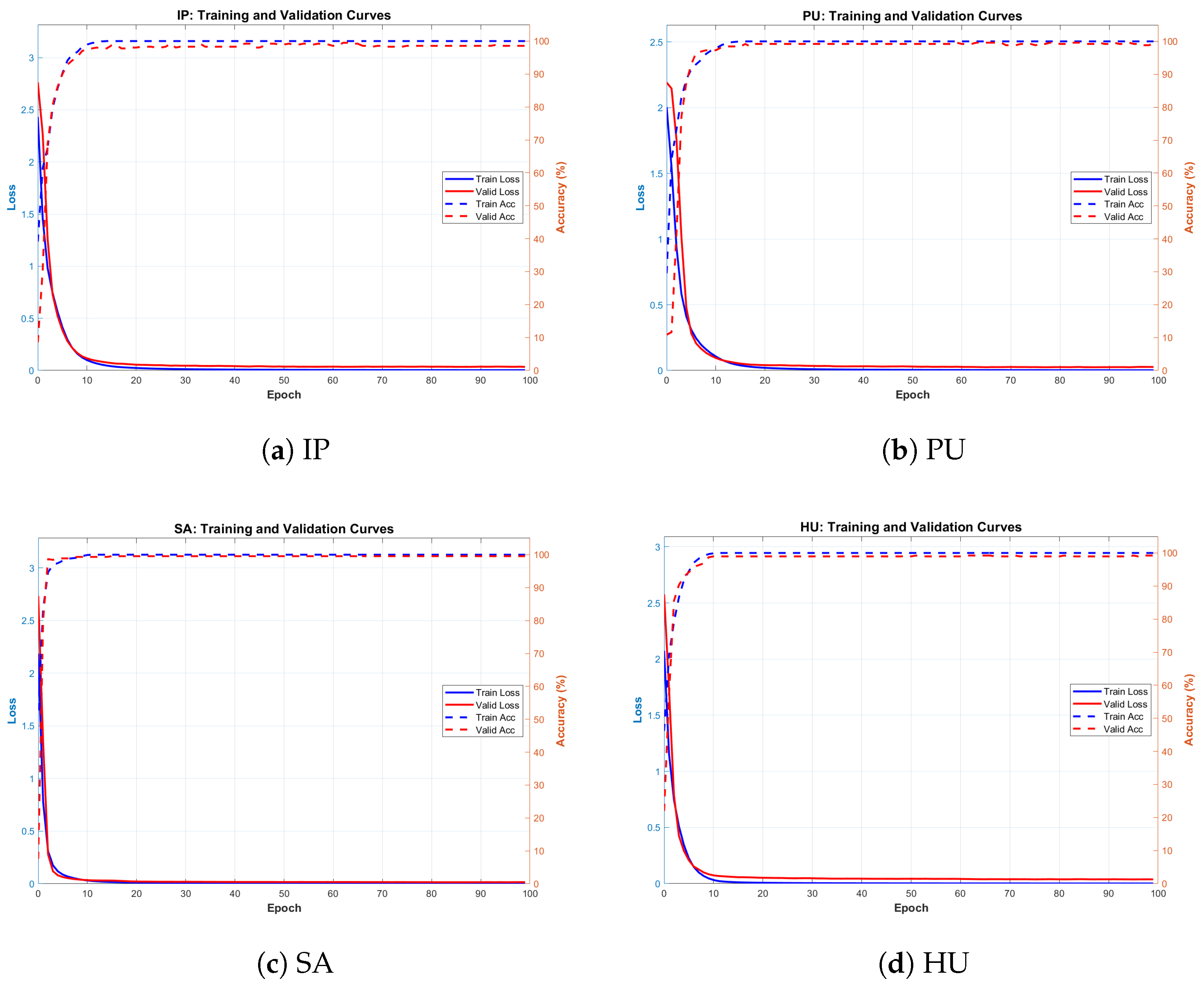
To further examine the training dynamics, Figure 3 shows the training and validation loss and accuracy curves over 100 epochs on all four datasets. The model converges within approximately 30–40 epochs, and validation accuracy stabilizes at competitive levels (above $97\%$ on IP and HU, above $98\%$ on PU and SA). No notable overfitting is evident, as the gap between training and validation curves remains consistently small. This demonstrates the effectiveness of the training configuration and the model’s strong generalization across diverse hyperspectral scenes, from heterogeneous vegetation (IP) and urban areas (PU, HU) to homogeneous agricultural regions (SA).

3.3. Evaluation Metrics

Two categories of metrics are used to evaluate the proposed method: classification accuracy metrics and efficiency metrics.

3.3.1. Classification Accuracy Metrics

Three standard metrics are used to assess classification performance:

• Overall Accuracy (OA): proportion of correctly classified samples.
• Average Accuracy (AA): mean of per-class accuracies, providing a balanced view on imbalanced datasets.
• Kappa coefficient (κ): measure of classification consistency accounting for chance agreement.

3.3.2. Efficiency Metrics

To assess the applicability of the model to resource-constrained deployments, three efficiency metrics are employed.

• Parameter count: the total number of trainable parameters, indicating model complexity and memory footprint.
• Synaptic operations (SOPs): the total number of synaptic activations during the inference process, which directly reflects the computational complexity of the spike-driven models. Unlike the floating-point operations (FLOPs) used in ANNs, SOPs only count the spike-triggered events, which is aligned with the event-driven nature of SNNs.
  For a convolutional layer, $\mathrm{SOPs}$ are calculated as:

  $${\mathrm{SOP}}_{\mathrm{Conv}}^{\left(l\right)}=T·B·\left({\displaystyle \frac{C_{\mathrm{in}}^{\left(l\right)}}{g^{\left(l\right)}}}·K_h{K}_w·C_{\mathrm{out}}^{\left(l\right)}·H_{\mathrm{out}}^{\left(l\right)}{W}_{\mathrm{out}}^{\left(l\right)}\right),$$

  (21)

  where T is the number of time steps, B is the batch size, $C_{\mathrm{in}}^{\left(l\right)}$ and $C_{\mathrm{out}}^{\left(l\right)}$ are the input and output channels, $g^{\left(l\right)}$ is the number of groups in groupwise convolution, $K_h\times K_w$ is the kernel size, and $H_{\mathrm{out}}^{\left(l\right)}\times W_{\mathrm{out}}^{\left(l\right)}$ is the output spatial dimensions.
  For a linear layer, $\mathrm{SOPs}$ are calculated as:

  $${\mathrm{SOP}}_{\mathrm{Linear}}^{\left(l\right)}=T·B·D_{\mathrm{in}}^{\left(l\right)}·D_{\mathrm{out}}^{\left(l\right)},$$

  (22)

  where $D_{in}^{\left(l\right)}$ and $D_{out}^{\left(l\right)}$ are the input and output dimensions of the linear layer, respectively.
  The total $\mathrm{SOPs}$ are the sum over all convolutional and linear layers:

  $${\mathrm{SOP}}_{\mathrm{all}}=\sum _{l\in {\mathcal{L}}_{\mathrm{Conv}}}{\mathrm{SOP}}_{\mathrm{Conv}}^{\left(l\right)}+\sum _{l\in {\mathcal{L}}_{\mathrm{Linear}}}{\mathrm{SOP}}_{\mathrm{Linear}}^{\left(l\right)}.$$

  (23)
• Energy consumption: according to the convention in neuromorphic computing research [14,15,23,24], the theoretical energy consumption for inference is estimated based on SOPs. Using the standard energy model, each SOP consumes approximately $0.9$ mJ [15]. This value is derived from the estimated energy cost of addition operations in a typical 45 nanometer CMOS process and has been widely used for fair, hardware-agnostic comparisons of SNN models. Therefore, the energy calculation for each image is as follow:

  $$\mathrm{Energy}={\mathrm{SOP}}_{\mathrm{all}}\times 0.9\mathrm{mJ}.$$

  (24)
  It is worth noting that this is a theoretical upper-bound estimation, primarily intended for relative comparisons among different SNN architectures. The actual energy consumption of specific neuromorphic hardware may vary depending on the chip architecture, process node, and data encoding scheme. Nevertheless, this standardized estimation ensures fair and reproducible comparisons, as it has been consistently adopted in previous work [14,15,23,24].

3.4. Hyperparameter Analysis

In this section, the influence of four key hyperparameters on the classification performance is systematically assessed: spatial patch size, time steps T, the number of attention heads $\mathrm{n}\_\mathrm{h}$, and the number of groups g. When analyzing a single hyperparameter, the others are fixed at their default values: $T=4$, $heads=8$, $g=16$, and the input channel dimension of the Transformer stage is $C=64$. All reported results are the average values of ten independent runs.

3.4.1. Spatial Patch Size

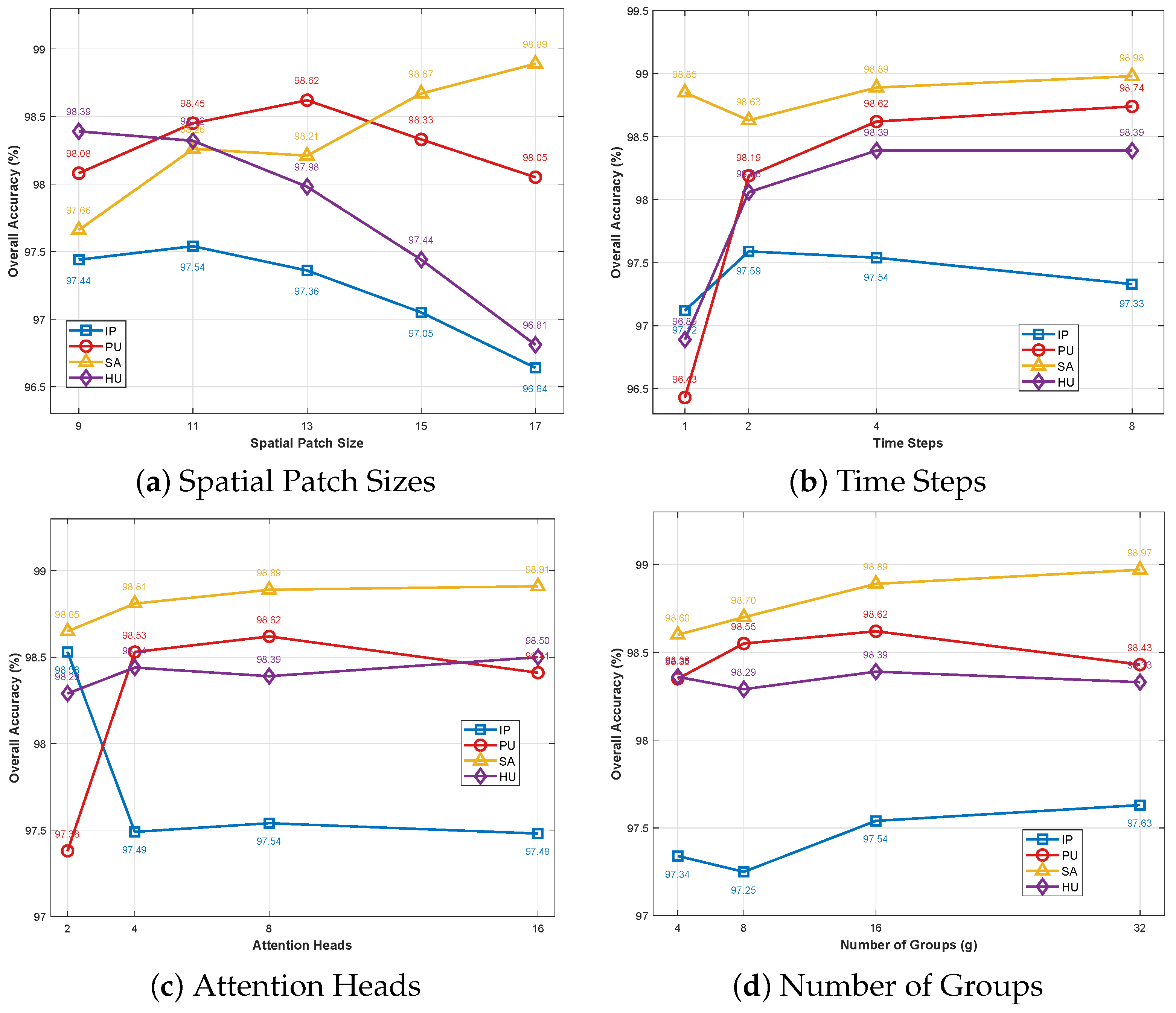
The spatial patch size determines the amount of context information used for classification. Patch sizes from $9\times 9$ to $17\times 17$ are evaluated, with the results summarized in Table 7 and Figure 4a.

The results reveal that the classification performance is highly sensitive to this hyperparameter. The optimal patch size varies substantially across different datasets, reflecting differences in scene structure. For the heterogeneous vegetation scene of IP, the peak performance is $11\times 11$, yielding an OA of $97.54\%$. Beyond this size, the performance gradually declines, indicating that larger patches will introduce redundant background information, which may confuse the classifier. The urban scene of PU dataset achieves its best OA of $98.62\%$ when the patch size is $13\times 13$. However, the accuracy declined afterwards, possibly due to the inclusion of mixed pixels from neighboring urban objects. In contrast, the homogeneous agricultural scene of SA benefits from a broader spatial context, with the largest patch size being $17\times 17$, resulting in the highest OA of $98.89\%$. The complex urban scene of HU performs the best, with the smallest patch size of $9\times 9$ (OA of $98.39\%$), indicating that finer spatial details are more crucial for distinguishing diverse urban land cover types.

As shown in Figure 4a, the OA curves for all datasets exhibit clear peaks, confirming that the accuracy typically increases with patch size up to a dataset-specific optimum. Beyond this value, due to redundant context or blurred boundaries, it tends to stabilize or decrease. Table 7 also reports the computational costs (training time, testing time, and SOPs) for each patch size. As expected, larger patch sizes lead to higher computational overhead. For example, on the IP dataset, increasing the patch size from $9\times 9$ to $17\times 17$ increases the SOPs from $0.100$ G to $0.382$ G. Nevertheless, the primary criterion for selecting the optimal patch size is classification accuracy. In the subsequent experiments, these optimal sizes are adopted: $11\times 11$ for IP, $13\times 13$ for PU, $17\times 17$ for SA, and $9\times 9$ for HU.

3.4.2. Number of Time Steps

The number of time steps T governs the trade-off between temporal integration and computational cost. For time steps $T=1,2,4,8$, the optimal patch size determined in the previous step is used for evaluation.

As shown in Table 8 and Figure 4b, increasing T generally improves the OA of all datasets, although the improvement rate varies, reflecting the differences in dataset complexity and temporal dynamics. For IP, the OA increases from $97.12\%$ at $T=1$ to $97.59\%$ at $T=2$, with a gain of $0.47\%$, which is the highest among all time steps. The slight decrease at $T=4$ ($97.54\%$) and $T=8$ ($97.33\%$) indicates that longer temporal simulations may introduce redundant spike activities, which is not conducive to the learning of distinguishing features for this heterogeneous vegetation scene. For PU, the OA continuously improves from $96.43\%$ at $T=1$ to $98.74\%$ at $T=8$ (with a total gain of $2.31\%$), indicating that the urban scenario of PU involves more complex temporal dynamics that benefits from a longer integration of spike information. For SA, the OA reaches $98.98\%$ at $T=8$, only $0.13\%$ higher than that at $T=4$ ($98.89\%$), suggesting that for this homogeneous agricultural scenario, the benefits decrease after exceeding $T=4$. For HU, the OA saturates at $T=4$ ($98.39\%$) with no further gain at $T=8$, suggesting that four time steps are sufficient to capture the discriminative features in this complex urban scenario.

In contrast, the computational costs of all datasets (measured in SOPs and estimated energy) increase linearly with T. On IP, the SOPs increase from $0.038$ G at $T=1$ to $0.307$ G at $T=8$ (an 8 fold increase), while OA only improves by $0.21\%$. Therefore, to balance accuracy and computational efficiency, $T=4$ is selected as the default configuration for the subsequent experiments.

3.4.3. Number of Attention Heads

Multi-head attention enables the model to capture diverse feature subspaces. The number of attention heads ranges from 2 to 16, while keeping $T=4$, $C=64$, $g=16$, and the optimal patch size.

As shown in Table 9 and Figure 4c, performance remains stable across different numbers of heads on all datasets (IP: $97.54\%$, PU: $98.62\%$, SA: $98.89\%$, HU: $98.39\%$), with $\mathrm{n}\_\mathrm{h}$ = 8 achieving the best or near-best OA. The OA varies only slightly among different head counts, typically within $0.2\%$ for each dataset. Taking IP as an example, the OA ranges from $97.48\%$ ($\mathrm{n}\_\mathrm{h}$ = 16) to $97.54\%$ ($\mathrm{n}\_\mathrm{h}$ = 8), a difference of merely $0.06\%$. Computational cost also shows negligible variation, as increasing the number of heads reduces the dimensionality per head ($d_h=C/n\_h$), keeping the total computational load approximately constant. Therefore, adopting 8 heads as the standard configuration provides a robust balance between representational diversity and computational efficiency.

3.4.4. Number of Groups

The group number g in the GSA module plays a crucial role in balancing parameter efficiency and feature extraction capability. By dividing the channels into independent groups in the self-attention projection, groupwise separable convolution substantially reduces parameters and computational costs while preserving the ability to model global dependencies. The group numbers are $g=4,8,16,32$, with $T=4$, $\mathrm{n}\_\mathrm{h}=8$, $C=64$, and the optimal patch size.

As shown in Table 10 and Figure 4d, the performance differences among different g values are marginal, typically within $0.3\%$ of each dataset. For IP, $g=32$ yields the highest OA ($97.63\%$), which is only $0.09\%$ higher than $g=16$ ($97.54\%$). For PU, $g=16$ achieves the best OA ($98.62\%$), $0.19\%$ lower than $g=32$. For SA, the results of $g=16$ (98.89%) and $g=32$ (98.97%) are comparable, with a difference of only $0.08\%$. For HU, $g=16$ achieves the best OA ($98.39\%$), $0.06\%$ lower than $g=32$. The results show that this model is robust to the choice of g. Due to the marginal performance differences and to maintain consistency across all datasets, the default configuration of $g=16$ is adopted.

3.4.5. Summary of Optimal Configuration

Based on the above analysis, all subsequent experiments adopt the following configuration. The spatial patch size is set to the optimal value for each dataset: IP is $11\times 11$, PU is $13\times 13$, SA is $17\times 17$, and HU is $9\times 9$. The remaining hyperparameters are fixed across all datasets: time steps $T=4$, the number of attention heads $heads=8$, and the groups $g=16$. This uniform configuration ensures fair comparisons while maintaining competitive performance, as the above analyses have demonstrated that the model is robust to variations in T, $\mathrm{n}\_\mathrm{h}$, and g within a reasonable range.

3.5. Ablation Study

To rigorously evaluate the contribution of each key component in the proposed GS-SpikeFormer framework, an ablation study is conducted on the IP dataset. All experiments follow the training scheme described in Section 3.4.

3.5.1. Variant Models

Three configurations are designed to systematically analyze the contributions:

• Baseline (SpikingResformer-HSI): Since the original SpikingResformer [15] is designed for high-resolution RGB images (e.g., $224\times 224$), it cannot be directly applied to small HSI patches (e.g., $11\times 11$). Therefore, it is suitable for a single-stage architecture and 64-channel HSIC tasks, denoted as ‘SpikingResformer-HSI’. This baseline implements the original Dual Spike Self-Attention (DSSA) mechanism in SpikingResformer [15], using running-average firing rate for scaling and standard ($1\times 1$) convolution for output projection. It employs a simple prologue consisting of a single ($3\times 3$) convolution, batch normalization, and max-pooling (with stride = 1). There is neither a proposed front-end module (such as Spectral Calibration or Spatial Calibration) nor any use of groupwise convolution.
• Baseline+Front-end: This configuration adds the recommended Spectral Calibration (SC) and Spatial Calibration (SP) modules to the baseline. The SC module consists of $1\times 1$ convolution (256 channels), followed by BN and spiking neuron activation; the SP module consists of $3\times 3$ convolution (64 channels), followed by BN, spiking neruron activation, and stride-1 max-pooling. These modules are inserted between the input and the prologue.
• Full Model: This is the complete proposed model. It further replaces DSSA with the GSA mechanism (using fixed scaling and groupwise separable convolutions in the output projection), and employs the GWSFFN. The front-end modules (SC + SP) are also included.

3.5.2. Results and Analysis

Table 11. Ablation Study on four Datasets.

Dataset	Config	OA (%)	AA (%)	$\mathit{\kappa }$ (×100)
IP (P = 11)	Baseline	95.69 ± 0.80	97.86 ± 0.45	95.02 ± 0.92
	+SC+SP	96.24 ± 0.75	98.11 ± 0.43	95.65 ± 0.87
	Full model	97.54 ± 0.58 *	98.45 ± 1.05	97.15 ± 0.67 *
PU (P = 13)	Baseline	97.92 ± 0.65	97.88 ± 0.43	97.24 ± 0.86
	+SC+SP	98.26 ± 0.37	98.09 ± 0.42	97.68 ± 0.49
	Full model	98.62 ± 0.37 *	98.23 ± 0.29 *	98.16 ± 0.49 *
SA (P = 17)	Baseline	98.84 ± 0.35	99.42 ± 0.24	98.71 ± 0.39
	+SC+SP	98.95 ± 0.56	99.52 ± 0.20	98.82 ± 0.63
	Full model	98.89 ± 0.52	99.56 ± 0.15	98.76 ± 0.58
HU (P = 9)	Baseline	97.89 ± 0.33	98.24 ± 0.33	97.71 ± 0.36
	+SC+SP	98.12 ± 0.57	98.44 ± 0.49	97.96 ± 0.62
	Full model	98.39 ± 0.41 *	98.62 ± 0.35 *	98.25 ± 0.44 *

Note: The ‘Baseline’ corresponds to SpikingResformer-HSI, which implements the original DSSA mechanism in SpikingResformer [15] and adapts to HSIC with a single-stage architecture. * $p<0.05$ vs. Baseline (paired t-test, 10 runs).

reports the quantitative results of the three configurations across all four datasets. The progressive improvements from the Baseline to the Baseline+Front-end and then to the Full Model consistently confirm the effectiveness of each proposed component.

• Contribution of Front-end modules: Adding the SC+SP modules to the Baseline can improve the performance of all datasets, and the magnitude of improvement reflects the complexity of the scenarios. On IP (heterogeneous vegetation, severe class imbalance), OA increases from $95.69\%$ to $96.24\%$ (a gain of $0.55\%$), AA increases from $97.86\%$ to $98.11\%$ (a gain of $0.25\%$), and $\kappa$ increases from $95.02\%$ to $95.65$ (a gain of $0.63\%$). The relatively larger gains indicate that the Front-end module is particularly beneficial for complex and imbalanced scenarios. On PU (urban scene), OA improves from $97.92\%$ to $98.26\%$ (a gain of $0.34\%$), confirming that these modules help capture discriminative features in urban environments. On SA (homogeneous agricultural scenario), OA increases from $98.84\%$ to $98.95\%$ (a gain of $0.11\%$), and the marginal gain is expected, as the Baseline has already achieved nearly saturated performance and there is little room for improvement. On HU (complex urban scenario), OA improves from $97.89\%$ to $98.12\%$ (a gain of $0.23\%$), confirming the effectiveness of these modules on challenging urban data. AA and $\kappa$ show similar trends across all datasets. These improvements verified that Front-end module effectively reduce spectral redundancy and enhance local spatial feature representation.
• Contribution of GSA and GWSFFN: Replacing DSSA with the proposed GSA and incorporating groupwise convolutions into the Feedforward network further improve the performance on most datasets. On IP, the Full Model achieves $97.54\%$ OA (an additional gain of $1.3\%$ over Baseline+Front-end), $98.45\%$ AA ($0.34\%$) and $97.15$$\kappa$ ($1.5\%$). The substantial gains demonstrate that GSA is particularly effective in capturing global spatial dependencies in challenging heterogeneous scenarios. On PU, OA reaches $98.62\%$ (a gain of $0.36\%$), confirming that GSA is also beneficial for urban scene classification. On SA, the Full Model achieves an OA of $98.89\%$, which is comparable within the standard deviation range to the Baseline+Front-end ($98.95\%$), indicating that the Baseline architecture has well-handled the dataset. On HU, OA reaches $98.39\%$ (a gain of $0.27\%$), highlighting the robustness of GSA in complex urban data. These results confirm that the proposed GSA not only reduces parameters through groupwise projections but also enhances the global context modeling ability. Meanwhile, GWSFFN effectively refines the local spectral-spatial features.

To rule out random variation, paired t-tests are conducted between the Full Model and the Baseline over 10 independent runs per dataset, separately for OA, AA, and $\kappa$. The results show that OA improvements are statistically significant ($p<0.05$) on IP ($p=0.00001$), PU ($p=0.002$), and HU ($p=0.008$), while SA shows no significant improvement ($p=0.46$), which is consistent with the near-saturated performance on this homogeneous agricultural scene. For AA and $\kappa$, PU and HU show significant improvements, while SA does not. On IP, thought OA and $\kappa$ show significant improvements, AA does not ($p=0.418$), which may be attributed to the severe class imbalance of this dataset. These results confirm that the proposed components consistently enhance performance on challenging datasets while remaining competitive on already well-solved scenarios.

In summary, the ablation studies demonstrate that each of the proposed components contributes meaningfully to the performance of GS-SpikeFormer. The Front-end modules enhance the input representation, while GSA and GWSFFN jointly achieve efficient global and local feature learning within a fully spike-driven framework.

4. Comparison with SNN-Based HSIC Methods

In this section, the proposed GS-SpikeFormer is evaluated against two representative HSIC methods based on SNN: SNN-SSEM [12] and AFSA [14]. SNN-SSEM [12] is a conventional SNN built on LIF neurons with direct coding. It is trained with approximate gradient methods and employs standard convolutions alongside spiking depthwise separable convolutions for spectral-spatial feature extraction. Lacking attention mechanisms, it typically requires a large number of time steps to achieve competitive accuracy. AFSA [14] represents a recent attempt to integrate attention-like mechanisms into SNNs for HSIC. It introduces a spike self-attention (SSA) module coupled with adaptive refocusing convolutional layers. While AFSA incorporates attention-inspired components, it remains largely within the conventional spike-driven paradigm without fully embracing the Transformer architecture, and still requires careful tuning, particularly under very low time step settings. For AFSA, the original network structure is followed with the same $75/25$ training/validation split as used for all other methods (see Section 3.1) to ensure fair comparison. While AFSA’s original paper [14] reports higher accuracy with 100 training samples per class, the unified protocol adopted here allows a consistent evaluation across all models. In contrast, GS-SpikeFormer fully embeds Transformer principles within a SNN framework, building upon the spiking Transformer backbone of SpikingResformer [15] while optimizing it for efficient spike-compatible global dependency modeling tailored to hyperspectral data.

All models are trained and evaluated under the identical training strategy and evaluation metrics, with dataset-specific optimal patch sizes. The results of the configurations across multiple time step are reported in

Table 12. Comparison with SNN-Based HSIC Methods on IP dataset over different time steps.

Time Steps	SNN-Based Methods	OA (%)	AA (%)	$\mathit{\kappa }$ (×100)	Training Time (s)	Test Time (s)	Infer Time (×10−4 s)	SOPs (G)	Energy (mJ)	Param (M)
1	SNN-SSEM	-	-	-	-	-	-	-	-	-
	AFSA	91.84 ± 1.01	96.13 ± 0.37	90.59 ± 1.14	30.08 ± 0.53	1.06 ± 0.03	1.19	0.12149	0.10934	3.52
	GS-SpikeFormer	97.12 ± 0.53	98.56 ± 0.24	96.66 ± 0.62	22.25 ± 0.68	0.61 ± 0.00	0.69	0.03831	0.03448	0.35
2	SNN-SSEM	86.43 ± 2.84	93.14 ± 1.90	84.38 ± 3.26	36.53 ± 1.03	1.54 ± 0.05	1.73	0.07570	0.06813	0.86
	AFSA	89.99 ± 1.85	92.59 ± 2.61	88.46 ± 2.11	49.61 ± 0.93	1.63 ± 0.03	1.83	0.23535	0.21182	3.52
	GS-SpikeFormer	97.59 ± 0.49	98.77 ± 0.23	97.21 ± 0.56	27.88 ± 0.80	0.83 ± 0.01	0.93	0.07663	0.06897	0.35
4	SNN-SSEM	91.51 ± 1.51	95.58 ± 0.58	90.19 ± 1.32	61.08 ± 0.56	2.46 ± 0.17	2.77	0.15001	0.13501	0.86
	AFSA	93.29 ± 0.88	96.57 ± 0.55	92.25 ± 1.01	86.84 ± 0.28	2.68 ± 0.01	3.01	0.46308	0.41677	3.52
	GS-SpikeFormer	97.54 ± 0.58	98.45 ± 1.05	97.15 ± 0.67	47.78 ± 1.03	1.33 ± 0.03	1.50	0.15326	0.13793	0.35
8	SNN-SSEM	93.20 ± 0.97	96.71 ± 0.69	92.15 ± 1.11	112.14 ± 0.91	4.17 ± 0.10	4.69	0.29861	0.26875	0.86
	AFSA	95.11 ± 0.71	97.63 ± 0.24	94.34 ± 0.81	162.21 ± 2.18	4.78 ± 0.05	5.38	0.91853	0.82667	3.52
	GS-SpikeFormer	97.33 ± 0.36	98.48 ± 0.61	96.91 ± 0.41	82.76 ± 1.32	2.16 ± 0.01	2.43	0.30651	0.27586	0.35

,

Table 13. Comparison with SNN-Based HSIC Methods on PU dataset over different time steps.

Time Steps	SNN-Based Methods	OA (%)	AA (%)	$\mathit{\kappa }$ (×100)	Training Time (s)	Test Time (s)	Infer Time (×10−4 s)	SOPs (G)	Energy (mJ)	Param (M)
1	SNN-SSEM	-	-	-	-	-	-	-	-	-
	AFSA	96.88 ± 0.78	97.22 ± 0.31	95.85 ± 1.03	19.38 ± 0.20	5.53 ± 0.11	1.32	0.17060	0.15354	2.26
	GS-SpikeFormer	96.43 ± 1.19	96.61 ± 0.73	95.27 ± 1.57	16.99 ± 0.66	3.52 ± 0.04	0.84	0.05420	0.04878	0.35
2	SNN-SSEM	96.12 ± 1.02	96.33 ± 0.56	94.86 ± 1.31	25.99 ± 0.28	7.6 ± 0.17	1.81	0.10671	0.09604	0.87
	AFSA	95.35 ± 3.05	94.76 ± 3.07	93.86 ± 3.98	32.51 ± 1.44	8.16 ± 0.31	1.95	0.33059	0.29753	2.26
	GS-SpikeFormer	98.19 ± 0.67	97.88 ± 0.55	97.59 ± 0.89	24.86 ± 0.68	5.44 ± 0.07	1.30	0.10840	0.09756	0.35
4	SNN-SSEM	97.48 ± 0.66	97.59 ± 0.32	96.64 ± 0.86	42.37 ± 0.23	11.58 ± 0.13	2.77	0.21148	0.19033	0.87
	AFSA	97.27 ± 1.06	97.19 ± 0.57	96.37 ± 1.40	54.69 ± 0.25	12.80 ± 0.10	3.06	0.65058	0.58552	2.26
	GS-SpikeFormer	98.62 ± 0.37	98.23 ± 0.29	98.16 ± 0.49	42.50 ± 0.67	9.15 ± 0.05	2.19	0.21681	0.19513	0.35
8	SNN-SSEM	97.41 ± 0.93	97.62 ± 0.55	96.56 ± 1.23	75.14 ± 0.17	19.38 ± 0.07	4.63	0.42101	0.37891	0.87
	AFSA	97.64 ± 0.73	97.66 ± 0.91	96.86 ± 0.97	104.06 ± 1.77	22.58 ± 0.09	5.39	1.29055	1.16149	2.26
	GS-SpikeFormer	98.74 ± 0.35	98.41 ± 0.22	98.32 ± 0.46	77.85 ± 1.21	15.19 ± 0.08	3.63	0.43362	0.39026	0.35

,

Table 14. Comparison with SNN-Based HSIC Methods on SA dataset over different time steps.

Time Steps	SNN-Based Methods	OA (%)	AA (%)	$\mathit{\kappa }$ (×100)	Training Time (s)	Test Time (s)	Infer Time (×10−4 s)	SOPs (G)	Energy (mJ)	Param (M)
1	SNN-SSEM	62.83 ± 39.03	66.81 ± 39.72	60.80 ± 40.16	39.17 ± 0.48	9.11 ± 0.33	1.73	0.09451	0.08506	0.91
	AFSA	98.54 ± 0.60	99.35 ± 0.20	98.37 ± 0.67	47.82 ± 0.55	10.84 ± 0.48	2.06	0.28115	0.25303	2.32
	GS-SpikeFormer	98.85 ± 0.29	99.51 ± 0.12	98.72 ± 0.32	50.23 ± 0.61	8.43 ± 0.12	1.61	0.09495	0.08546	0.35
2	SNN-SSEM	97.65 ± 0.65	98.92 ± 0.30	97.38 ± 0.73	55.30 ± 0.25	11.92 ± 0.18	2.27	0.18569	0.16712	0.91
	AFSA	96.94 ± 1.74	98.44 ± 0.74	96.59 ± 1.93	76.93 ± 1.11	16.06 ± 0.29	3.06	0.54416	0.48975	2.32
	GS-SpikeFormer	98.63 ± 0.55	99.44 ± 0.25	98.47 ± 0.61	85.65 ± 0.66	14.07 ± 0.06	2.68	0.18990	0.17091	0.35
4	SNN-SSEM	98.45 ± 0.64	99.34 ± 0.19	98.27 ± 0.72	86.59 ± 0.22	16.69 ± 0.09	3.18	0.36804	0.33124	0.91
	AFSA	98.36 ± 0.49	99.23 ± 0.24	98.17 ± 0.54	139.22 ± 2.00	27.24 ± 0.50	5.19	1.07019	0.96317	2.32
	GS-SpikeFormer	98.89 ± 0.52	99.56 ± 0.15	98.76 ± 0.58	156.03 ± 0.45	25.49 ± 0.09	4.85	0.37980	0.34182	0.35
8	SNN-SSEM	98.38 ± 0.68	99.32 ± 0.27	98.19 ± 0.76	151.06 ± 0.79	26.32 ± 0.06	5.01	0.73275	0.65948	0.91
	AFSA	98.68 ± 0.44	99.44 ± 0.19	98.53 ± 0.49	262.25 ± 0.38	49.08 ± 0.03	0.34	2.12226	1.91003	2.32
	GS-SpikeFormer	98.98 ± 0.36	99.57 ± 0.09	98.87 ± 0.40	293.14 ± 1.28	43.50 ± 0.09	8.28	0.75960	0.68364	0.35

and

Table 15. Comparison with SNN-Based HSIC Methods on HU dataset over different time steps.

Time Steps	SNN-Based Methods	OA (%)	AA (%)	$\mathit{\kappa }$ (×100)	Training Time (s)	Test Time (s)	Infer Time (×10−4 s)	SOPs (G)	Energy (mJ)	Param (M)
1	SNN-SSEM	-	-	-	-	-	-	-	-	-
	AFSA	96.19 ± 0.56	96.81 ± 0.48	95.87 ± 0.60	29.30 ± 0.33	1.42 ± 0.03		0.07983	0.07983	3.52
	GS-SpikeFormer	96.89 ± 0.55	97.46 ± 0.53	96.63 ± 0.59	24.58 ± 0.66	0.88 ± 0.01	0.65	0.02493	0.02244	0.35
2	SNN-SSEM	92.92 ± 1.28	94.04 ± 1.03	92.34 ± 1.38	36.61 ± 0.28	2.04 ± 0.04	1.51	0.04947	0.04452	0.86
	AFSA	95.95 ± 0.65	96.34 ± 0.50	95.62 ± 0.71	48.86 ± 0.24	2.22 ± 0.01	1.64	0.15457	0.13912	3.52
	GS-SpikeFormer	98.06 ± 0.39	98.37 ± 0.37	97.90 ± 0.43	24.79 ± 0.67	0.99 ± 0.01	0.73	0.04987	0.04488	0.35
4	SNN-SSEM	95.54 ± 0.59	96.21 ± 0.53	95.17 ± 0.64	64.20 ± 0.95	3.36 ± 0.08	2.48	0.09801	0.08820	0.86
	AFSA	97.10 ± 0.34	97.50 ± 0.29	96.86 ± 0.37	87.04 ± 0.48	3.78 ± 0.02	2.79	0.30406	0.27365	3.52
	GS-SpikeFormer	98.39 ± 0.41	98.62 ± 0.35	98.25 ± 0.44	33.76 ± 0.69	1.36 ± 0.00	1.00	0.09973	0.08976	0.35
8	SNN-SSEM	96.73 ± 0.64	97.22 ± 0.58	96.46 ± 0.69	117.14 ± 0.37	5.90 ± 0.03	4.36	0.19508	0.17557	0.86
	AFSA	97.37 ± 0.45	97.70 ± 0.48	97.15 ± 0.49	166.72 ± 0.93	7.07 ± 0.03	5.22	0.60304	0.54273	3.52
	GS-SpikeFormer	98.39 ± 0.50	98.62 ± 0.46	98.26 ± 0.54	57.42 ± 1.56	2.16 ± 0.01	1.60	0.19946	0.17952	0.35

, where the entries marked with ‘-’ indicate that the training process did not converge to a specific configuration.

Across all the dataset and time step configurations, GS-SpikeFormer consistently outperforms the two baselines in terms of accuracy, parameter efficiency, computational cost, and inference speed. It is noteworthy that GS-SpikeFormer achieves strong performance even in a single time step ($T=1$), demonstrating the effectiveness of attention mechanism in SNNs for HSIC under low time step settings. Represented by the IP dataset, at $T=4$, GS-SpikeFormer achieves an OA of $97.54\%$, which is $6.03\%$ higher than SNN-SSEM ($91.51\%$) and $4.25\%$ higher than AFSA ($93.29\%$). It only uses $0.35$ M parameters, which is 60–$90\%$ less than SNN-SSEM ($0.86$ M) and AFSA ($3.52$ M). In terms of computational cost, GS-SpikeFormer requires $0.153$ G SOPs, which is comparable to SNN-SSEM ($0.15$ G, only $2\%$ higher) but $67\%$ lower than AFSA ($0.463$ G). Despite its slightly higher SOPs than SNN-SSEM, GS-SpikeFormer achieves $46\%$ faster inference ($1.5\times {10}^{-4}$ s vs. $2.77\times {10}^{-4}$ s), indicating that its lightweight groupwise separable attention mechanism can make better use of the hardware. Similar trends are also observed on the HU, SA and HU datasets, as detailed in Table 12, Table 13, Table 14 and Table 15.

Overall, GS-SpikeFormer achieves a superior trade-off between accuracy and efficiency. Even in a single time step, it can deliver powerful performance, using 60–$90\%$ fewer parameters than the baselines while maintaining or slightly exceeding the SOPs of SNN-SSEM (with much higher accuracy), and achieving 46–$64\%$ faster inference. Compared to AFSA, GS-SpikeFormer reduces the computational cost by 62–$67\%$ and achieves 50–$64\%$ faster inference while maintaining superior accuracy. These results indicate that the proposed architecture is highly suitable for resource-constrained edge deployment.

5. Comparison with SOTA HSIC Methods

The proposed GS-SpikeFormer is evaluated against various state-of-the-art methods, including CNN-based (PResNet [25] and HybridSN [26]), Transformer-based (SSFTT [27] and GSC-VIT [9]), and SNN-based (SNN-SSEM [12] and AFSA [14]).

This comparison situates the model in a broader high-accuracy HSIC context and demonstrates its competitiveness beyond the SNN domain. All models are trained and evaluated under the same experimental protocol to ensure fair comparisons. For SNN-based methods, the original time step settings are as follows: SNN-SSEM [12] uses 30 steps, AFSA [14] uses 1 step, and the proposed GS-SpikeFormer uses 4 steps. The results are averaged over 10 runs and reported with standard deviations.

5.1. Results on Indian Pines (IP)

Table 16. Classification Results of different methods for the IP dataset.

Class No.	CNN-Based		Transformer-Based		SNN-Based		GS-SpikeFormer
	PResNet	HybridSN	SSFTT	GSC-ViT	SNN-SSEM	AFSA
1	96.67	98.89	100.00	100.00	100.00	100.00	100.00
2	73.63	85.05	92.00	94.07	90.66	88.10	95.84
3	78.85	91.26	95.84	97.37	95.21	92.42	98.56
4	97.23	98.83	99.78	99.78	100.00	99.05	100.00
5	93.39	96.32	97.31	97.70	97.08	95.74	97.81
6	98.79	99.44	99.83	99.25	99.40	97.68	99.51
7	100.00	100.00	100.00	100.00	100.00	100.00	100.00
8	99.89	99.76	100.00	99.92	100.00	99.58	100.00
9	92.50	100.00	100.00	100.00	100.00	100.00	95.00
10	80.31	88.02	93.85	95.53	93.23	90.89	96.24
11	72.90	82.61	89.98	93.59	92.07	86.08	96.32
12	78.62	89.35	95.88	96.21	95.76	93.81	97.02
13	99.71	99.43	99.81	99.24	99.43	99.05	99.62
14	95.90	96.39	98.71	99.02	98.40	96.83	99.43
15	97.41	96.01	99.44	99.86	98.99	98.81	99.79
16	99.44	99.44	100.00	98.33	99.44	100.00	100.00
OA (%)	82.99 ± 1.41	89.95 ± 1.30	94.66 ± 0.79	96.25 ± 0.50	94.80 ± 1.13	91.84 ± 1.01	97.54 ± 0.58
AA (%)	90.95 ± 1.49	95.05 ± 0.61	97.65 ± 0.30	98.12 ± 0.25	97.48 ± 0.56	96.13 ± 0.37	98.45 ± 1.05
$\kappa$ ($\times 100$)	80.50 ± 1.59	88.30 ± 1.48	93.83 ± 0.90	95.66 ± 0.57	93.98 ± 1.30	90.59 ± 1.14	97.15 ± 0.67

summarize the results on the IP dataset. GS-SpikeFormer achieves an OA of $97.54\%$, outperforming all compared methods. It substantially surpasses CNN-based models (PResNet: $82.99\%$, HybridSN: $89.95\%$) by $14.55\%$ and $7.59\%$, respectively, demonstrating the advantage of spike-driven attention over conventional convolutions in heterogeneous agricultural scenarios. Among Transformer-based methods, GS-SpikeFormer exceeds SSFTT ($94.66\%$) by $2.88\%$ and GSC-Vit ($96.25\%$) by $1.29\%$, confirming the effectiveness of the proposed Gated Spiking Attention in capturing both global dependencies and local spectral-spatial features while maintaining fully spike-drive computation. Against SNN-based methods, it outperforms SNN-SSEM ($94.80\%$) by $2.74\%$ and AFSA ($91.84\%$) by $5.70\%$. Notably, these gains are achieved with only $T=4$ time steps, a substantial reduction from SNN-SSEM’s $T=30$ steps, highlighting the model’s superior temporal efficiency.

Per-class analysis reveals consistent gains on challenging categories. For Class 2 (Corn-notill), GS-SpikeFormer reaches $95.84\%$, compared to $90.66\%$ for SNN-SSEM and $88.1\%$ for AFSA. For Class 11 (Soybean-mintill), it attains $96.32\%$, versus $92.07\%$ and $86.08\%$, respectively. These gains are particularly significant given the limited training samples for these classes, underscoring the model’s ability to distinguish spectrally similar agricultural categories.

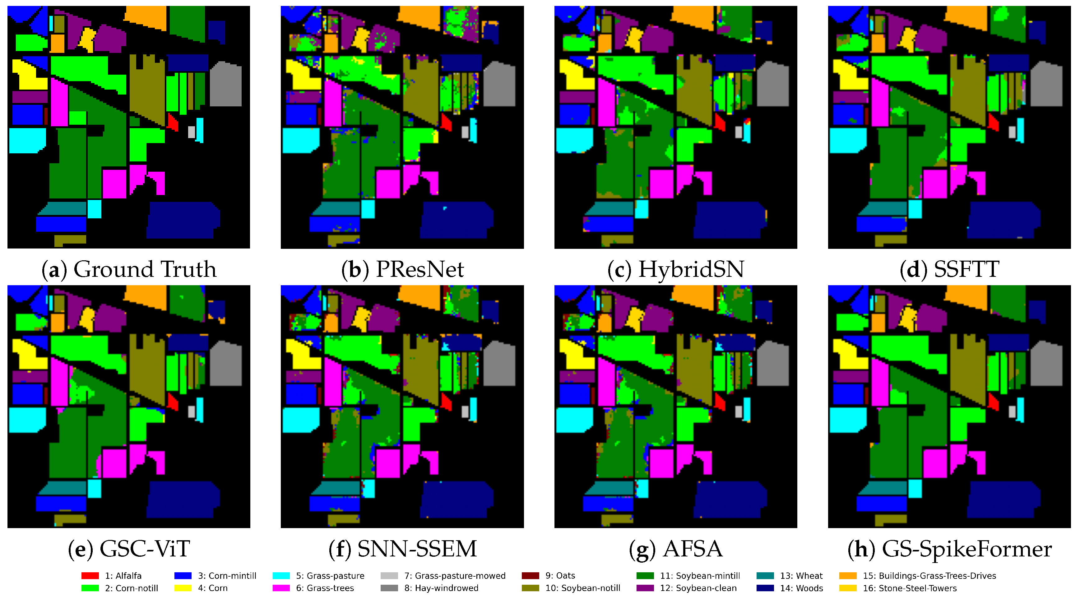
The classification map in Figure 5 shows cleaner boundaries and fewer misclassifications, especially along field edges, corroborating the quantitative results.

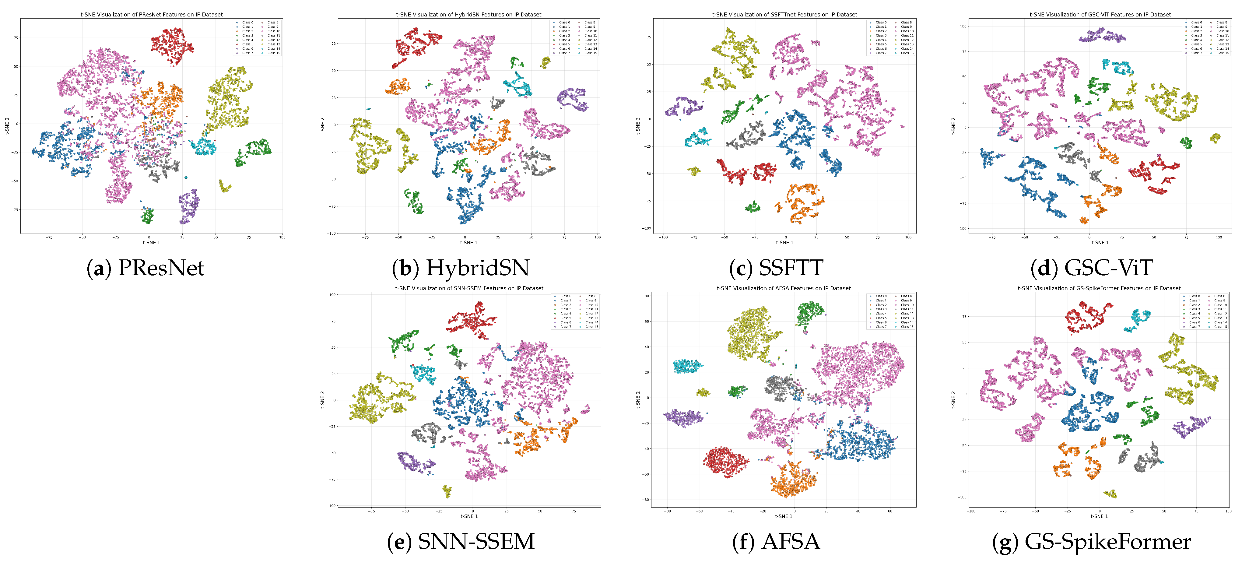
To intuitively assess feature discriminability, t-SNE visualization is performed on the IP dataset (Figure 6). Features extracted by GS-SpikeFormer form more compact and well-separated clusters than those from the competing methods, exhibiting clearer class boundaries and fewer inter-class overlaps. In contrast, CNN-based (PResNet, HybridSN) and Transformer-based (SSFTT, GSC-ViT) methods show relatively scattered distributions. Among SNN-based methods, AFSA yields moderately separated clusters, whereas GS-SpikeFormer achieves the most discriminative feature space. These results confirm that the proposed GSA mechanism and groupwise convolutions effectively learn more discriminative spectral-spatial representations than existing methods.

5.2. Results on Pavia University (PU)

On the PU dataset (

Table 17. Classification Results of different methods for the PU dataset.

Class No.	CNN-Based		Transformer-Based		SNN-Based		GS-SpikeFormer
	PResNet	HybridSN	SSFTT	GSC-ViT	SNN-SSEM	AFSA
1	87.95	94.60	96.39	94.76	97.91	95.35	97.48
2	95.94	94.81	98.13	97.97	97.43	97.21	99.48
3	91.12	94.07	97.09	96.62	97.50	94.68	96.94
4	95.02	96.39	97.10	95.02	97.44	96.88	95.30
5	99.92	99.99	99.91	99.57	99.88	99.92	99.73
6	98.26	96.86	98.89	99.76	99.28	98.47	99.57
7	99.11	99.06	99.84	99.70	99.79	99.70	99.95
8	85.75	90.69	95.90	93.59	96.24	94.58	97.97
9	97.39	99.24	98.42	97.13	99.00	98.22	97.66
OA (%)	94.04 ± 1.49	95.11 ± 1.48	97.74 ± 1.02	97.12 ± 0.94	97.80 ± 1.46	96.88 ± 0.83	98.62 ± 0.37
AA (%)	94.50 ± 0.88	96.19 ± 0.96	97.96 ± 0.55	97.13 ± 0.31	98.27 ± 0.52	97.22 ± 0.32	98.23 ± 0.29
$\kappa$ ($\times 100$)	92.12 ± 1.92	93.54 ± 1.92	97.00 ± 1.34	96.17 ± 1.22	97.08 ± 1.89	95.85 ± 1.08	98.16 ± 0.49

), GS-SpikeFormer achieves the highest OA of $98.62\%$, outperforming all compared methods. Specifically, it surpasses the CNN-based methods PResNet ($94.04\%$) and HybridSN ($95.11\%$) by $4.58\%$ and $3.51\%$, respectively, demonstrating the effectiveness of spike-driven attention in capturing discriminative features in urban scenes. Among Transformer-based models, GS-SpikeFormer exceeds SSFTT ($97.74\%$) by $0.88\%$ and GSC-ViT ($97.12\%$) by $1.50\%$, confirming the advantage of the proposed GSA over conventional self-attention and its grouped variants. Compared to SNN-based approaches, GS-SpikeFormer achieves gains of $0.82\%$ over SNN-SSEM ($97.80\%$) and $1.74\%$ over AFSA ($96.88\%$), highlighting its superior accuracy within the SNN domain.

A closer examination of per-class performance reveals both strengths and nuanced trade-offs. GS-SpikeFormer achieves outstanding results on several challenging urban categories. For instance, on Class 2 (Meadows), it attains $99.48\%$, the highest among all methods, significantly outperforming PResNet ($95.94\%$) and HybridSN ($94.81\%$). Similarly, on Class 7 (Bitumen), it achieves $99.94\%$, surpassing all competitors, with the closest being SSFTT at $99.95\%$. These results indicate the model’s strong capability in distinguishing spectrally distinct land-cover classes with sufficient training samples.

However, on Class 4 (Trees), GS-SpikeFormer yields $95.30\%$, which is lower than SNN-SSEM ($97.44\%$) and AFSA ($96.88\%$). This suggests that while the proposed model excels in many categories, certain classes may benefit from alternative architectural designs or different temporal integration strategies. Similarly, on Class 9 (Bare Soil), GS-SpikeFormer achieves $97.66\%$, slightly below the best-performing method SNN-SSEM ($99.00\%$). These observations indicate that despite achieving the highest overall accuracy, the model does not uniformly dominate all classes, and the gains in OA are driven by substantial improvements in categories with larger sample sizes (e.g., Classes 2, 5, 6, 7) rather than marginal improvements across all classes.

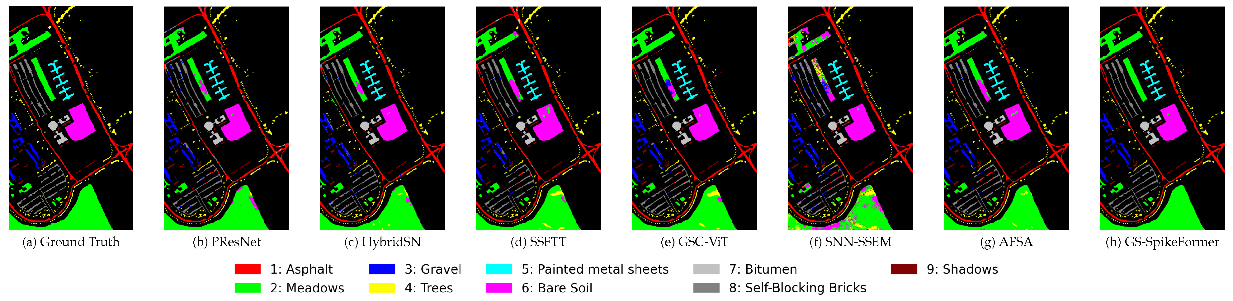
The classification map in Figure 7 visually corroborates these quantitative findings. GS-SpikeFormer produces sharper boundaries and fewer misclassifications in homogeneous areas such as ‘meadows’ and ‘bitumen’, while showing minor irregularities in tree-covered regions.

5.3. Results on Salinas (SA)

For the SA dataset (

Table 18. Classification Results of different methods for the SA dataset.

Class No.	CNN-Based		Transformer-Based		SNN-Based		GS-SpikeFormer
	PResNet	HybridSN	SSFTT	GSC-ViT	SNN-SSEM	AFSA
1	99.98	99.99	100.00	99.96	100.00	100.00	100.00
2	99.99	99.86	100.00	99.99	99.93	99.97	100.00
3	100.00	99.85	99.99	100.00	100.00	99.97	100.00
4	99.70	99.77	99.55	99.39	99.66	99.88	99.71
5	98.98	98.70	98.72	98.41	99.22	99.23	98.94
6	99.97	99.94	99.96	99.84	99.95	99.92	99.91
7	99.98	99.97	99.98	99.96	99.93	99.74	100.00
8	94.50	93.07	95.73	96.52	96.31	95.11	95.69
9	99.99	99.80	99.99	99.96	99.99	99.97	100.00
10	99.18	98.12	99.07	99.22	98.87	98.79	99.72
11	99.90	100.00	99.90	99.75	100.00	99.87	99.95
12	99.68	99.98	99.96	99.99	99.99	99.93	99.98
13	99.98	99.78	99.87	99.66	99.69	99.85	99.99
14	99.86	99.73	99.82	99.81	99.79	99.55	99.94
15	98.73	96.43	98.06	98.57	98.76	98.14	99.20
16	99.70	99.07	99.85	99.83	99.86	99.70	99.99
OA (%)	98.52 ± 0.64	97.77 ± 0.52	98.68 ± 0.61	98.88 ± 0.44	98.90 ± 0.44	98.54 ± 0.63	98.89 ± 0.52
AA (%)	99.38 ± 0.22	99.00 ± 0.26	99.40 ± 0.22	99.43 ± 0.16	99.50 ± 0.20	99.35 ± 0.21	99.56 ± 0.15
$\kappa$ ($\times 100$)	98.35 ± 0.72	97.52 ± 0.57	98.53 ± 0.68	98.76 ± 0.49	98.78 ± 0.50	98.37 ± 0.70	98.76 ± 0.58

), GS-SpikeFormer achieves an OA of $98.89\%$, which is comparable to SNN-SSEM ($98.90\%$) as the difference is well within the standard deviation range. This near-saturation performance is expected given the homogeneous agricultural nature of SA and the abundance of training samples. While the absolute gains are modest, this is expected given the near-saturation performance of all methods on SA, which features homogeneous agricultural scenes with relatively abundant training samples.

Per-class analysis reveals that GS-SpikeFormer achieves near-perfect accuracy on the majority of classes, with perfect scores on Classes 1, 2, 3, 7, 9 and 16. However, on Class 8 (Grapes-untrained), it reaches $95.69\%$, slightly below GSC-ViT ($96.52\%$) and SNN-SSEM ($96.31\%$). On Class 5 (Broccoli-green-weeds-1), it yields $98.94\%$, trailing SNN-SSEM ($99.22\%$) and AFSA ($99.23\%$). These minor trade-offs suggest that while the model excels overall, further refinement may be needed for specific classes with distinct spectral signatures.

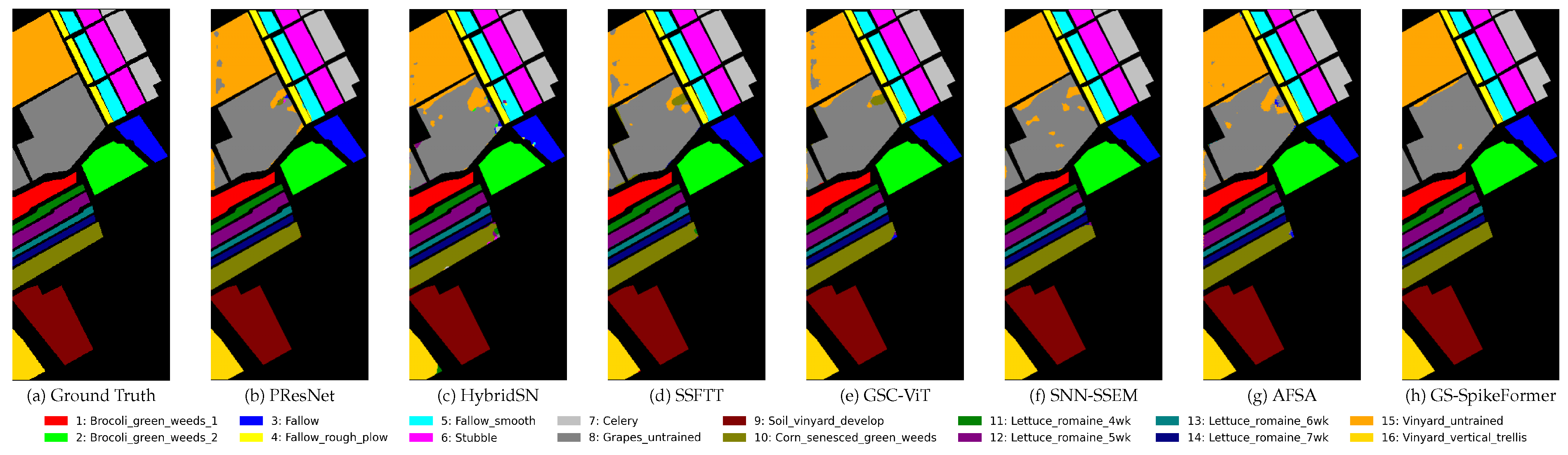
The classification map in Figure 8 shows well-delineated agricultural regions with high regional consistency, visually confirming the model’s robustness in homogeneous scenes.

5.4. Results on Houston2013 (HU)

On the challenging HU dataset (

Table 19. Classification Results of different methods for the HU dataset.

Class No.	CNN-Based		Transformer-Based		SNN-Based		GS-SpikeFormer
	PResNet	HybridSN	SSFTT	GSC-ViT	SNN-SSEM	AFSA
1	97.30	97.89	98.39	98.22	98.10	97.58	98.97
2	98.42	98.97	99.29	98.86	98.80	98.17	98.62
3	99.51	99.21	99.66	99.78	99.46	99.53	99.85
4	96.54	98.38	98.97	98.99	98.67	96.04	98.68
5	99.96	99.97	100.00	100.00	99.96	99.84	100.00
6	99.29	99.91	99.96	99.87	99.51	99.51	99.51
7	91.47	93.22	95.74	96.31	95.99	92.48	97.73
8	90.04	91.18	93.97	95.30	92.99	91.71	95.24
9	88.94	91.12	93.73	94.88	94.58	90.08	94.82
10	96.97	98.41	98.73	99.31	98.75	97.28	99.98
11	96.68	98.50	99.64	99.84	99.37	97.18	98.93
12	95.62	96.81	97.78	98.89	98.31	96.18	98.74
13	94.58	96.40	98.67	96.83	98.35	96.78	98.29
14	99.94	99.63	99.85	99.97	100.00	99.79	100.00
15	99.96	99.77	100.00	99.98	99.95	100.00	100.00
OA (%)	95.74 ± 0.52	96.83 ± 0.55	97.97 ± 0.49	98.25 ± 0.27	97.85 ± 0.55	96.19 ± 0.59	98.39 ± 0.41
AA (%)	96.35 ± 0.50	97.29 ± 0.42	98.29 ± 0.40	98.47 ± 0.26	98.19 ± 0.49	96.81 ± 0.51	98.62 ± 0.35
$\kappa$ ($\times 100$)	95.38 ± 0.56	96.56 ± 0.59	97.75 ± 0.53	98.10 ± 0.30	97.67 ± 0.60	95.87 ± 0.64	98.25 ± 0.44

, GS-SpikeFormer achieves an OA of $98.39\%$, outperforming all comparison methods. It outperformed the CNN-based models PResNet ($95.74\%$) and HybridSN ($96.83\%$) by $2.65\%$ and $1.56\%$ respectively, demonstrating strong generalization ability in this complex urban scene with extremely scarce samples (only $2.26\%$ of pixels labeled). In the Transformer-based methods, GS-SpikeFormer surpasses SSFTT ($97.97\%$) by $0.42\%$ and GSC-ViT ($98.25\%$) by $0.14\%$. Against the SNN-based methods, it outperforms SNN-SSEM ($97.85\%$) by $0.54\%$ and AFSA ($96.19\%$) by $2.2\%$.

Per-class analysis reveals both strengths and nuanced trade-offs. GS-SpikeFormer achieves the highest accuracy on several challenging categories, including Class 1 (Grassland: $98.97\%$), Class 3 (Synthetic Grass: $99.85\%$), and Class 7 (Water: $97.73\%$), and Class 10 (Residential: 99.98%). Notably, on Class 7, it substantially outperforms SSFTT ($95.74\%$) and AFSA ($92.48\%$), underscoring the model’s ability to capture fine spectral differences with limited samples. However, on Class 8 (Commercial) and Class 9 (Road), GS-SpikeFormer achieves $95.24\%$ and $94.82\%$, respectively, slightly trailing GSC-ViT ($95.30\%$ and $94.88\%$). These minor discrepancies suggest that while the proposed model excels in overall accuracy, further architectural refinements may benefit specific urban classes with highly heterogeneous spectral signatures.

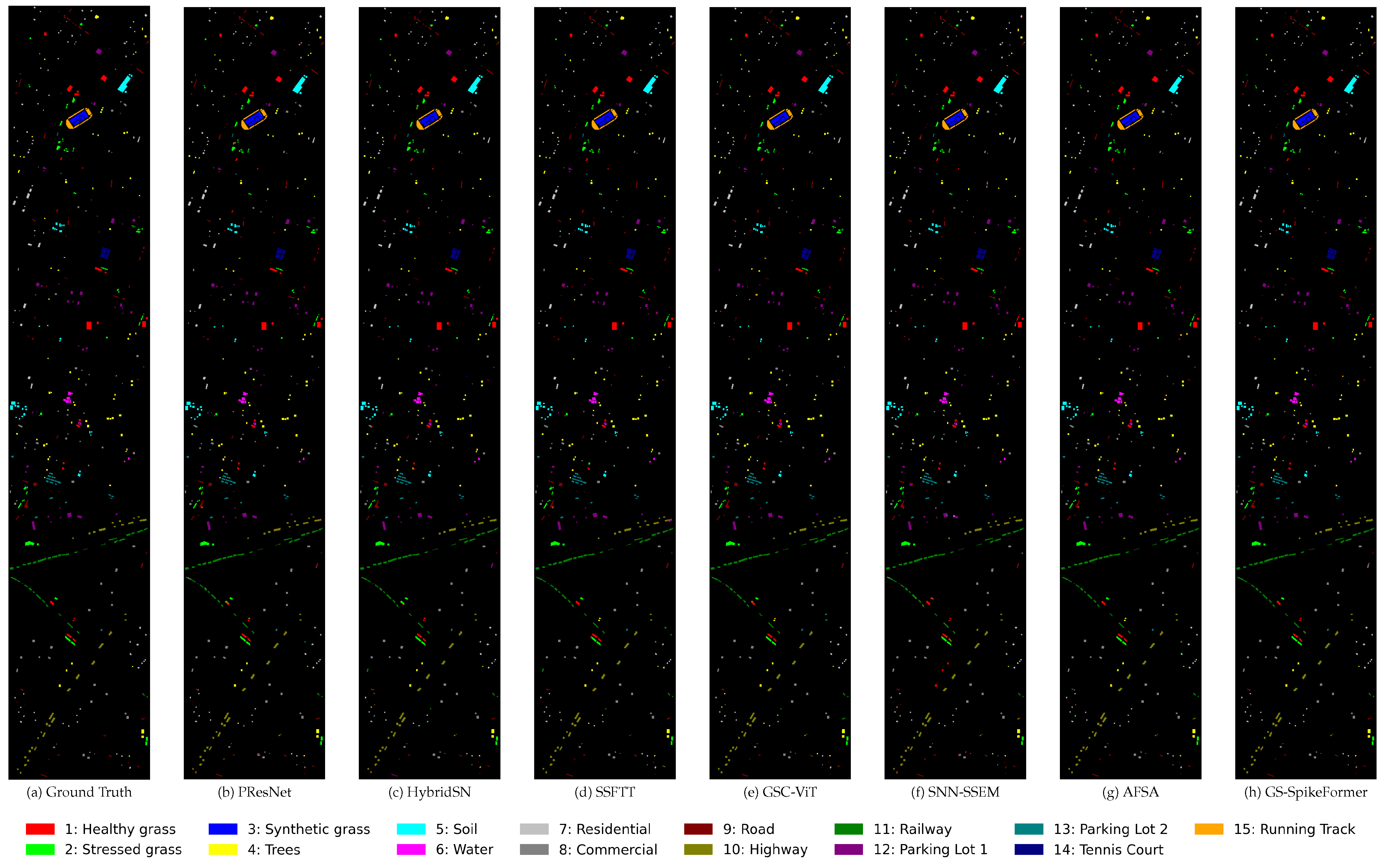
The classification map in Figure 9 reveals sharper boundaries and fewer errors in heterogeneous urban areas, visually confirming the model’s robustness.

6. Discussion

The experimental results demonstrate that GS-SpikeFormer achieves leading classification accuracy on four benchmark hyperspectral datasets using only 4 time steps and $0.35$ M parameters. This strongly supports the core hypothesis that multiply-accumulate operations in self-attention can be replaced by event-driven logical AND gating without compromising global context modeling. Compared to earlier SNN-based methods that rely on a large number of time steps (e.g., SNN-SSEM [12] requires 30 time steps, AFSA [14] demands careful tuning), the proposed GSA improves the OA on IP dataset by more than $6\%$ at extremely low time steps while reducing parameters by 60–$90\%$, validating the effectiveness of a spiking-compatible Transformer for HSIC. Even when compared with state-of-the-art convolutional and Transformer models such as PResNet [25], HybridSN [26], SSFTT [27], and GSC-VIT [9], GS-SpikeFormer attains higher accuracy than almost all datasets, indicating that the synergy between groupwise convolutions and binary attention gates not only preserves local spectral-spatial feature extraction capabilities but also offers inherent advantages for hardware-efficient deployment.

In a broader context, the model achieves $98.39\%$ OA on HU dataset with only $2.26\%$ labeled pixels and an estimated energy consumption as low as $0.09$ mJ per image, making it a promising candidate for real-time or onboard processing on resource-constrained platforms. Nevertheless, several limitations exist. The optimal spatial patch size varies across datasets (from $9\times 9$ to $17\times 17$), indicating that some degree of dataset-specific tuning is still required. For classes with severe imbalance (e.g., Oats in IP, Trees in PU), the fixed 4 time steps encoding occasionally underperforms certain baselines, suggesting that the current temporal coding strategy may not be sufficient for all land-cover types. Moreover, the reported energy consumption is a theoretical upper bound based on 45 nm CMOS assumptions, and actual energy efficiency on physical neuromorphic hardware remains to be validated.

Potential uncertainties in the results stem primarily from the randomness of limited-sample partitioning and the higher variance of rare classes. The class-aware splitting strategy guarantees a minimum number of training samples per class, but for extremely small classes the $60/20/20$ split may yield test subsets with limited representativeness. The selection of optimal hyperparameters depends on the validation set, introducing minor partition-related biases. The theoretical energy estimation assumes that every spike triggers a synaptic operation, without accounting for actual sparse activity patterns and hardware-specific optimizations, and should therefore be regarded as an upper-bound reference.

Future work may pursue several directions: designing an adaptive time-step mechanism that dynamically adjusts T based on input complexity to further balance accuracy and efficiency; deploying and benchmarking GS-SpikeFormer on neuromorphic chips such as Loihi or TrueNorth to obtain real-world energy measurements; exploiting the interpretable binary masks generated by GSA for spectral-spatial feature attribution analysis, thereby bridging high-performance models and explainable AI in remote sensing; extending the framework to multi-source and multi-temporal HSI data, as well as downstream tasks such as target detection and change detection; and combining the proposed architecture with advanced training paradigms such as STDP-based fine-tuning or few-shot meta-learning to further push the performance boundaries under extreme label scarcity. Overall, GS-SpikeFormer provides an accuracy-efficiency co-optimized spiking Transformer baseline for edge-oriented HSIC, while its current limitations outline a clear roadmap for subsequent refinement and broader adoption.

7. Conclusions

In this study, we introduced GS-SpikeFormer, a lightweight and fully spike-driven Vision Transformer architecture designed to address the dual challenges of high-dimensional data and limited labeled samples in HSIC. At the core of our method lies the novel Gated Spiking Self-Attention (GSA) mechanism, which adapts the efficient grouping principle of groupwise separable convolution to the spiking domain by reformulating the spiking-driven self-attention. This key innovation, together with a Front-end processing and the GWSFFN, enables the joint extraction of local spectral-spatial features and global contextual dependencies within a fully spike-compatible paradigm. Extensive experiments on four benchmark HSI datasets demonstrate that GS-SpikeFormer achieves state-of-the-art or highly competitive classification accuracy while substantially improving model efficiency. Notably, the model attains superior performance with very few training samples and reduces the parameter count to only $0.35$ M. More importantly, by maintaining end-to-end binary spike activations, our architecture preserves the event-driven, low-power characteristics of SNNs, making it highly suitable for deployment on resource-constrained edge devices. This work successfully bridges the gap between efficient group convolution design and spiking Transformer architectures, offering a practical pathway toward high-performance, low-power remote sensing systems.