Spatiotemporal Dynamics of Glacier Changes in Tibet from 1990 to 2025

Highlights

What are the main findings?

• An automated classification method based on GEE and random forests achieved high-precision extraction of glaciers in Tibet for the period 1990–2025, with an average overall accuracy of 92.10% across all time periods. The total glacier area decreased by approximately 43.5%, with retreat primarily concentrated in southeastern Tibet.
• Glacier area peaks at an elevation of 5500 m, with clean glaciers and debris-covered glaciers accounting for 42% and 55% of the total glacier area, respectively. The retreat rate exhibits a distinct spatial pattern of rapid retreat in the southeast and slow retreat in the northwest, and the Yarlung Tsangpo River basin experiences the fastest retreat, while the Qiangtang River basin shows signs of stabilization.

What are the implications of the main findings?

• This study provides reliable data and a reusable technical framework for large-scale, long-term monitoring of glacier dynamics in complex terrain, thereby lowering the economic and technical barriers to large-scale glacier mapping.
• It reveals the spatiotemporal response of Tibetan glaciers to climate change over the past 35 years, providing a scientific basis for regional water resource management and the development of climate change adaptation strategies.

Abstract

Glaciers serve as sensitive indicators of climate change, yet the automated extraction of glacier boundaries over large areas and long time periods remains challenging. To resolve this issue, we proposed a remote sensing indicator system based on the Google Earth Engine (GEE) platform (spectral, textural, topographic features and band differences) and applied a random forest (RF) algorithm to establish an automatic classification method. Based on this framework, the study analyzed the spatiotemporal changes in Tibet’s glaciers from 1990 to 2025. The results indicated that: (1) Validation using 30% of the data points showed overall accuracy (OA) was 92.10%, Kappa coefficient of 0.86 and F1-score of 91.53% for glacier classification. (2) The total glacier area retreated from 38,968 km² during 1990–1997 to 22,026 km² during 2024–2025, with the retreat mainly concentrated in southeastern Tibet. (3) Glacier area peaked at 5500 m, with clean glaciers and debris-covered glaciers accounting for 42% and 55% of the total glacier area, respectively. (4) Between 1990 and 2025, the Yarlung Tsangpo River basin exhibited the fastest glacier retreat rate, while the Qiangtang basin showed signs of stabilization. This study provides a theoretical basis for identifying glacier boundaries over large areas in high-altitude regions.

1. Introduction

The formation of glaciers involves extensive accumulation, compaction and refreezing of snow and ice [1]. As key indicators of climate change [2,3], glaciers are primarily found in high-altitude regions. As the core region of the “Water Tower of Asia”, Tibet is rich in glacial resources. Glacial variations in this region exert profound influences on both local and worldwide freshwater supply, climate regulation, cultural and tourism support, hydropower generation and carbon sequestration [4,5,6]. Therefore, comprehensive research on the dynamic changes of Tibet’s glaciers not only reveals fluctuations in glacier area but also provides data to estimate ice volume [7] and monitor changes in glacier mass [8]. This has important scientific and practical value for elucidating the underlying mechanisms of glacial changes in high-altitude regions and for formulating management strategies.

Glacier boundaries are critical for glaciological research and hydrological modeling. Therefore, ensuring high-precision glacier boundary detection is a prerequisite for studying glacier changes [9]. With advances in remote sensing technology, automated or semi-automated methods based on multispectral satellite imagery can be used to analyze dynamic changes in glacier area, such as the normalized difference snow index (NDSI) method [10], band ratio methods [11], object-oriented methods [12] and synthetic aperture radar (SAR) interferometry [13]. These methods are computationally simple and efficient, allowing rapid extraction of glacier area over large regions when applied to clean glaciers. However, NDSI and band ratio methods generally rely on empirical thresholds and are prone to interference from snow, clouds, shadows and water bodies, resulting in misclassification [14]. More importantly, the “spectrally similar but physically distinct” nature of debris-covered glaciers relative to the surrounding mountains and rocks makes the extraction of their boundaries challenging [15].

To further improve the accuracy of debris-covered glacier detection, researchers have proposed various methods. For example, they have developed a convolutional neural network (CNN) method specifically tailored for debris-covered glaciers: this method accurately identifies the boundaries of debris-covered glaciers and significantly reduces training time [16]. Other studies have utilized changes in coherence between SAR images [17], machine learning [18] and deep learning [19] to identify debris-covered glaciers. Although these algorithms and models have significantly improved the classification accuracy of debris-covered glaciers, the complex data acquisition and preprocessing processes limit their applicability to small-scale glacier extraction. Long-term glacier monitoring over large areas requires not only the processing and analysis of massive amounts of remote sensing imagery data but also the resolution of issues related to data formats and resolution. This undoubtedly presents significant economic and technical barriers to large-scale glacier change monitoring and analysis [20].

The advent of the GEE platform has facilitated large-scale mapping and the efficient processing of massive amounts of remote sensing data [21,22,23]. GEE can rapidly process and analyze pixel-level data to produce computational results and has found extensive application in monitoring climate change [24,25], land-use change [26,27], changes in surface water [28,29], and changes in snow and ice [14,30,31,32], among other applications. This provides effective technical support for large-scale glacier monitoring. However, in the automatic extraction of glacier boundaries over large areas, there is still room for improvement in the accurate identification of glaciers covered by moraines. Additionally, efforts are needed to reduce the influence of debris [33] and glacial lakes [34].

To address the challenges of glacier boundary extraction over large areas, this study proposed remote sensing indicators (spectral features, textural features, topographic features and band differences) for distinguishing between clean and debris-covered glaciers within the GEE platform. An automated classification method for large-scale glaciers was subsequently developed using the RF algorithm, and the extraction results were compared and analyzed against publicly available glacier datasets. Finally, the spatiotemporal variation characteristics of glaciers in Tibet from 1990 to 2025, as well as those of glaciers in different river basins were analyzed. This study provided data support and technical tools for the large-scale, long-term dynamic monitoring of glaciers.

2. Study Area and Data Sources

2.1. Study Area

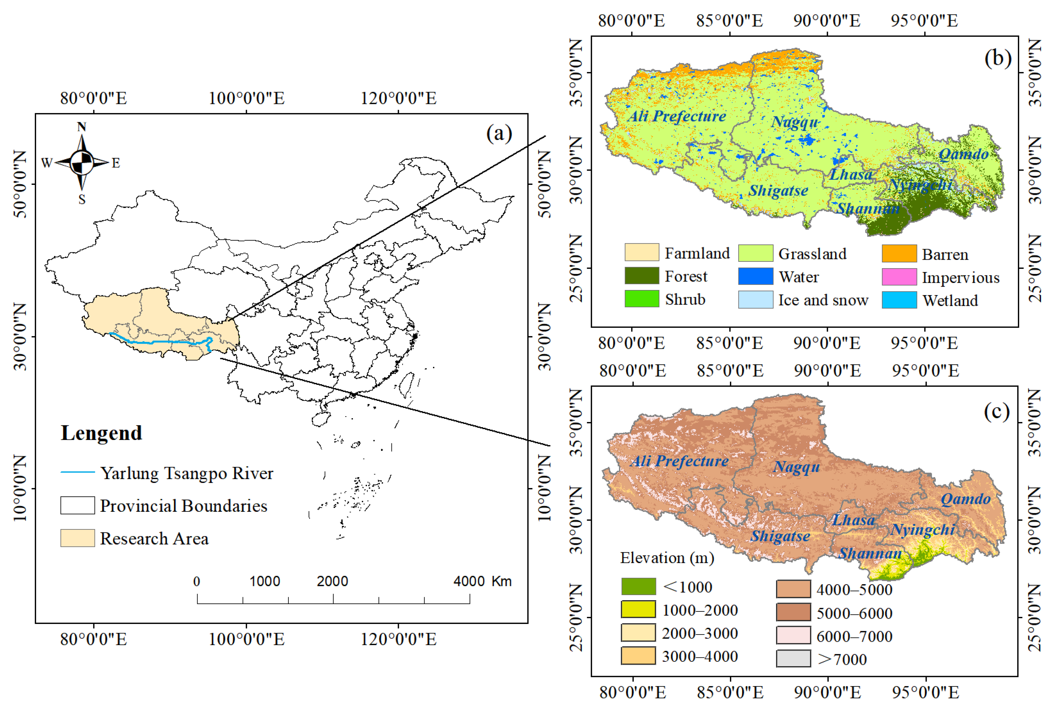
Tibet (26°50′–36°53′N, 78°25′–99°06′E) is located in western China (Figure 1a). With an average elevation exceeding 4000 m (Figure 1c), it is known as the “Roof of the World” and is the highest plateau on earth. The region covers an area of approximately 1.20 million square kilometers, accounting for 12.8% of China’s total land area. It is China’s second-largest provincial-level administrative region, comprising six prefectures and one autonomous prefecture (Figure 1b). The regional topography is dominated by plateau and mountainous terrain, with elevations higher in the northwest and lower in the southeast. Tibet’s climate, influenced by topography and atmospheric circulation, exhibits significant vertical differentiation and an east–west gradient. According to statistics from “Overview of Tibet,” Tibet’s average annual temperature ranges from −2.4 °C to 12.1 °C, and annual precipitation ranges from 66.3 to 894.5 mm. Tibet is a crucial water conservation area in China, with glacial reserves accounting for 46% of the national total [35]. The regional ecosystem is dominated by alpine meadows, grasslands, and bare ground, with a forest coverage rate of 9.11%.

2.2. Data Sources

The datasets used in this study include Landsat satellite remote sensing data, elevation data, land use data and glacier inventory data for result validation (

Table 1. Data sources and introduction.

Data Type	Data Resolution	Data Source
Landsat remote sensing data	30 m	https://earthexplorer.usgs.gov/
Land Use data	30 m	https://doi.org/10.5281/zenodo.12779975
Elevation data	30 m	http://www.gscloud.cn/
Glacier catalog dataset	/	A dataset of glacier inventory in western China during 2017–2018 (V1) [36]
	/	A new time-stamped glacier inventory of High Mountain Asia based on deep learning and remote sensing big data in 2020 [37]
	/	Randolph Glacier Inventory (RGI 7.0) (https://www.glims.org/)

).

3. Glacier Extraction Methods

3.1. Technical Approach

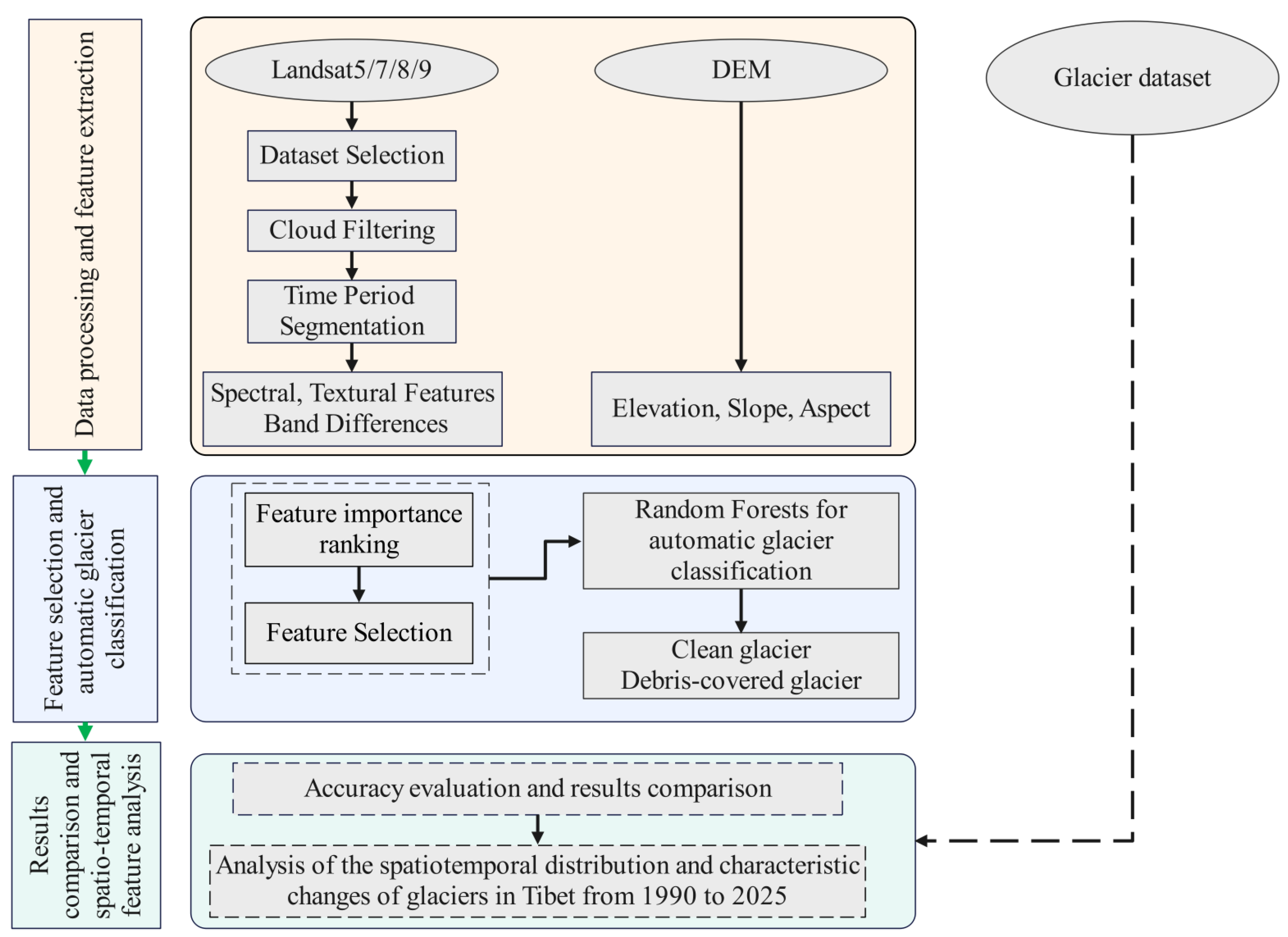
The approach of this study is based on GEE, which integrates spectral indices, texture indices, topographic features and band differences, and employs the RF method for automatic glacier classification. The specific technical workflow is shown in Figure 2.

3.2. Remote Sensing Data Preprocessing

3.2.1. Dataset Selection

This study selected Landsat series images from the summer melt season (June–October) for Tibet from 1990 to 2025. Because snow cover predominantly retreats during the summer, utilizing summer-season images effectively reduces the influence of snow.

3.2.2. Cloud Filtering

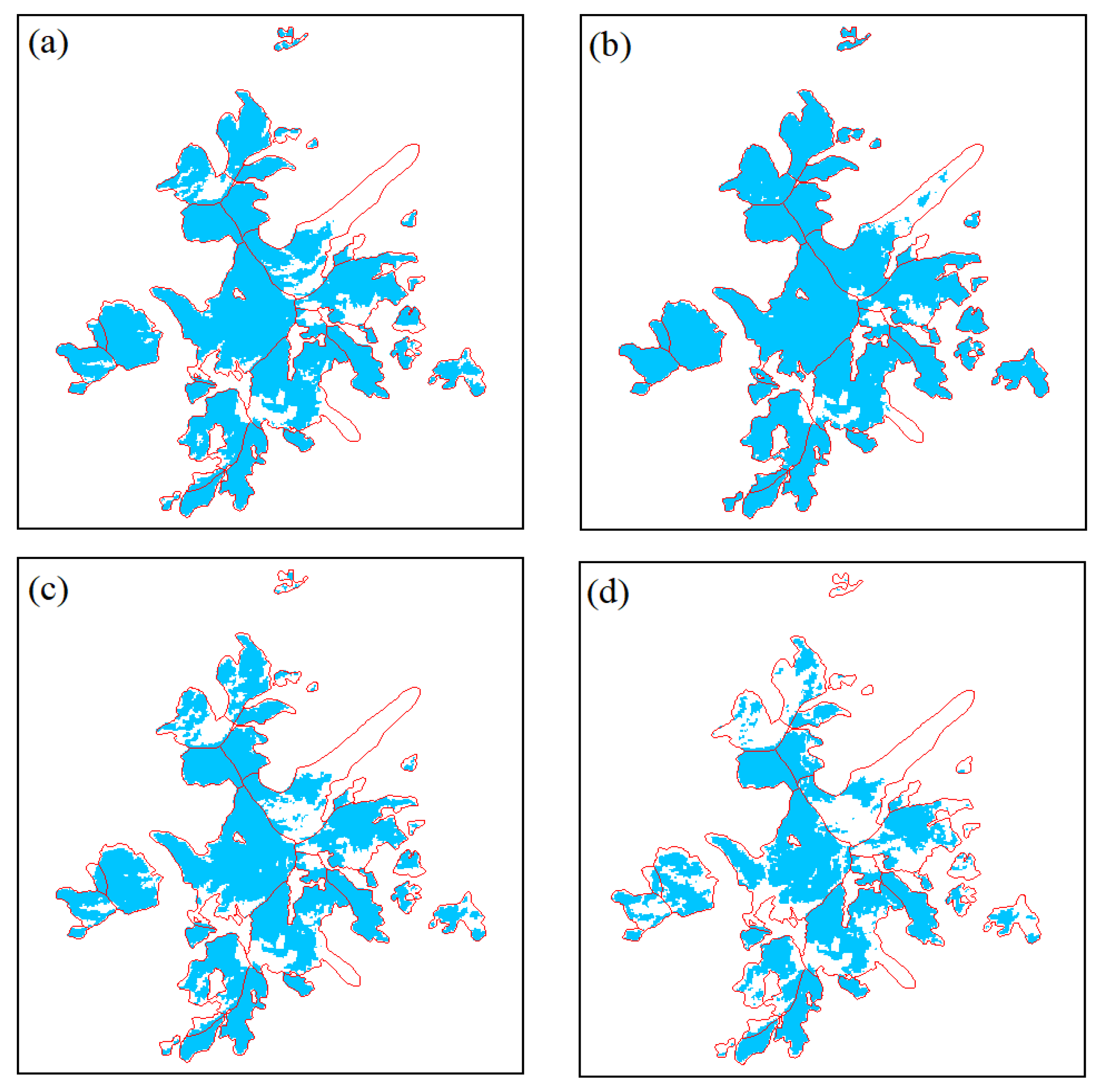
The GEE cloud scoring algorithm employed a filter to assign a cloud score to each pixel, ranging from 0 (cloud-free) to 100 (heavily clouded) [33]. When performing cloud removal filtering, setting the threshold too low reduces the number of usable pixels, leading to significant data gaps; conversely, setting the threshold too high allows thick clouds to obscure glacier features. The cloud score threshold that strikes a balance between these two extremes can be adopted as the threshold used in this study. Therefore, this study used the 2017–2018 western China glacier inventory dataset as a reference to compare the effects of different cloud score thresholds on glacier detection (Figure 3). The results revealed that a cloud score threshold of 60 achieved a balance the trade-off between empty pixels and cloud interference. Consequently, a cloud score of 60 was adopted for this study.

3.2.3. Method for Time Period Segmentation

After cloud filtering, the images may contain some empty pixels. Therefore, using only images from a single summer melt season may not be sufficient to generate a low-cloud, low-snow image of Tibet. Consequently, this study divided the period from 1990 to 2025 into several time segments to ensure that images from each segment could be combined into a complete low-cloud, low-snow image. Starting in 1990, imagery from successive years was added incrementally, and a composite image was generated to calculate its pixel loss rate. Once the composite image’s pixel loss rate fell below or equal to 1.0%, the division of that time period was considered finalized. Using this method, the period was ultimately divided into 10 segments, as shown in

Table 2. Time period segmentation.

Time Period	Image Category	Initial Number of Images	Number of Images After Cloud Filtering	Pixel Emptiness Rate
1990–1997	Landsat 5	1856	1439	0.21%
1998–2003	Landsat 5	1561	1073	0.27%
2004–2006	Landsat 7	1350	1051	0.84%
2007–2009	Landsat 7	1116	937	0.77%
2010–2013	Landsat 7	1957	1547	0.50%
2014–2016	Landsat 8	2107	1502	0.18%
2017–2018	Landsat 8	1384	919	1.00%
2019–2021	Landsat 8	2059	1448	0.74%
2022–2023	Landsat 9	1395	956	0.89%
2024–2025	Landsat 9	1362	951	0.87%

.

3.3. Feature Construction

3.3.1. Spectral Features

This study calculated various feature indices suitable for glacier identification. The Normalized Difference Snow Index (NDSI) serves as a common metric for snow/ice identification. Since snow and ice exhibit high reflectance in the visible spectrum but low reflectance in the shortwave infrared band, NDSI thresholding is applied to identify snow and ice through the difference in reflectance between these two bands. Although the Normalized Difference Vegetation Index (NDVI) does not directly identify glaciers, snow typically yields negative NDVI values due to its high reflectance in the red band, which can assist in distinguishing seasonal snow cover from permanent glaciers. The Normalized Difference Water Index (NDWI) highlights water bodies and helps avoid misidentifying moraine-dammed lakes at glacier termini as glaciers. The mathematical expressions for these three indices are provided below:

$$\mathrm{NDVI}={\displaystyle \frac{{\mathsf{\rho }}_{\mathrm{NIR}}-{\mathsf{\rho }}_{\mathrm{red}}}{{\mathsf{\rho }}_{\mathrm{NIR}}+{\mathsf{\rho }}_{\mathrm{red}}}}$$

(1)

$$\mathrm{NDSI}={\displaystyle \frac{{\mathsf{\rho }}_{\mathrm{green}}-{\mathsf{\rho }}_{\mathrm{SWIR}1}}{{\mathsf{\rho }}_{\mathrm{green}}+{\mathsf{\rho }}_{\mathrm{SWIR}1}}}$$

(2)

$$\mathrm{NDWI}={\displaystyle \frac{{\mathsf{\rho }}_{\mathrm{green}}-{\mathsf{\rho }}_{\mathrm{NIR}}}{{\mathsf{\rho }}_{\mathrm{green}}+{\mathsf{\rho }}_{\mathrm{NIR}}}}$$

(3)

where ${\mathsf{\rho }}_{\mathrm{red}},{ \mathsf{\rho }}_{\mathrm{green}},{ \mathsf{\rho }}_{\mathrm{NIR}},{ \mathsf{\rho }}_{\mathrm{SWIR}1}$ represent the red, green, near-infrared and short-wave infrared bands, respectively.

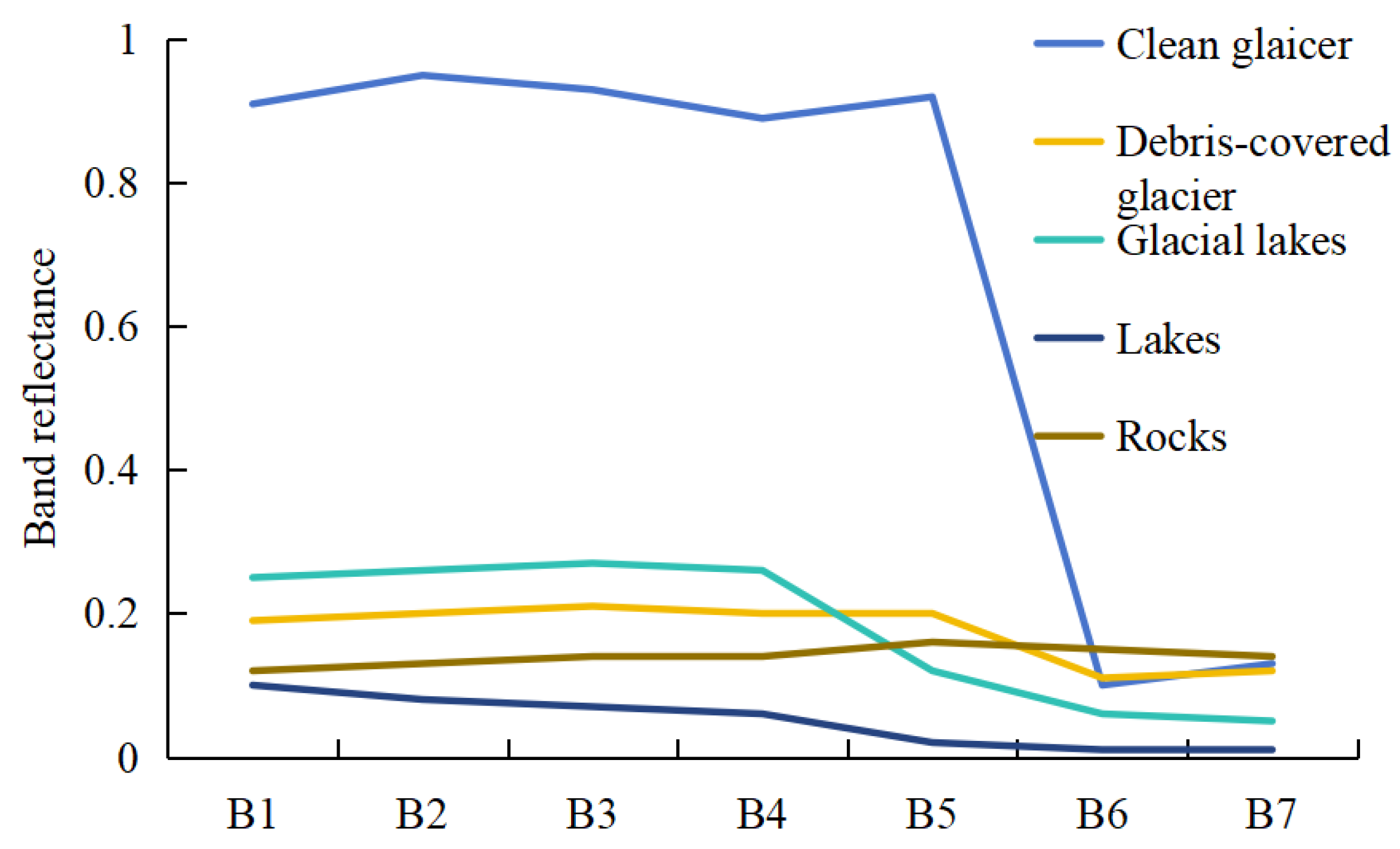
In addition, to distinguish between features with highly similar spectral signatures, such as debris-covered glaciers, bedrock and glacial lakes. This study used Landsat 8 imagery to sample debris-covered glaciers, bedrock, glacial lakes, lakes and clean glaciers in Tibet, and calculated the average reflectance for each land cover type, as shown in Figure 4. Clean glaciers, debris-covered glaciers, and non-glacial features (glacial lakes, lakes and rocks) exhibit substantial reflectance discrepancies in the near-infrared band (B5), whereas these differences diminish in the short-wave infrared band (B6). Therefore, this study proposes a band difference index (Diff_NIR_SWIR, B5-B6) to separate glaciers from non-glacier features.

3.3.2. Textural Features

Texture features represent information regarding the spatial arrangement and distribution of the elementary units in an image. This texture data is independent of color and brightness and serves as a complement to the image’s spectral information. Texture features contribute to a more complete understanding of an image; a full understanding can only be achieved by considering both its spectral and textural aspects [38]. The Gray-Level Co-occurrence Matrix (GLCM), introduced by Haralick in 1973, is a widely adopted method for texture description that analyzes spatial correlations among gray levels [39]. Texture features calculated using the GLCM have been widely applied in the analysis, classification, and interpretation of remote sensing data. This study utilized the texture feature calculation functions provided by GEE to compute eight commonly used texture features, including Mean, Variance (Var), Homogeneity (Hom), Contrast (Con), Dissimilarity (Dis), Entropy (Ent), Second Moment (SM) and Correlation (Cor).

3.3.3. Topographic Features

Topographic features are key indicators of ground elevation and surface morphology. In this study, the GEE cloud platform was used to calculate three topographic features: elevation, slope and aspect.

3.4. Feature Extraction

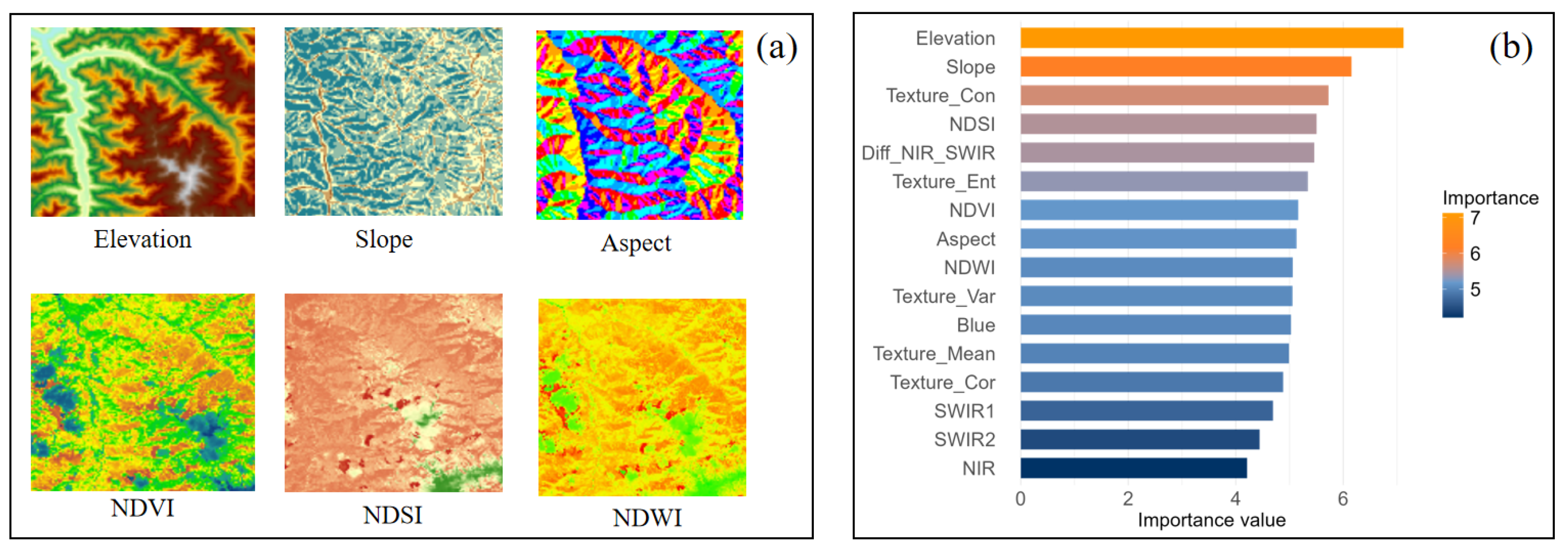
The incorporation of spectral indices, textural and topographic features markedly enhance the precision of glacier classification, the extraction of some feature indices is shown in Figure 5a. Additionally, this study aimed to address the issues of data redundancy and reduced computational efficiency caused by the large volume of multi-feature data while ensuring the accuracy of glacier extraction. First, the importance scores of all feature indices were calculated using the explain function of GEE. Second, features with the lowest importance scores were sequentially removed, and after each removal, the model’s overall classification accuracy and performance were re-evaluated on the current feature subset. Finally, by iteratively refining the feature combination, the process was halted when the overall classification accuracy and performance stabilized, ultimately selecting the 16 features that contributed most significantly to the model as inputs for the final modeling.

As shown in Figure 5b, the selected 16 features exhibit clear differences in their importance rankings. Among them, Elevation has the highest contribution, indicating that changes in elevation play a decisive role in distinguishing between glacial and non-glacial landforms. Slope and texture features follow closely behind. In terms of spectral features, spectral indices such as NDSI, NDVI and NDWI, as well as band difference indices, also exhibit high importance.

3.5. Glacier Boundary Extraction Based on RF

The method of aggregating multiple classifier models to improve classification or prediction accuracy is known as the bagging algorithm, with the most representative example of this is the RF algorithm, which was proposed by Leo Breiman [40]. RF combines outputs from numerous decision trees to form a single prediction. The classification performance of RF primarily depends on two parameters: the number of trees (Ntree) and the number of features used (Mtry). The Ntree value was incrementally increased from 0 to 100 in steps of 1, with the classification accuracy recorded at each step. Model accuracy peaked when Ntree was around 30, while the Mtry parameter was set to the square root of the total feature count in the training dataset [41]. Furthermore, compared to traditional machine learning algorithms, RF also offers significant advantages in terms of computational efficiency [42]. As machine learning classifiers rely on labeled training data, this study selected samples of clean glaciers, debris-covered glaciers, and non-glacial features (glacial lakes, lakes, rocks, vegetation) through visual interpretation. The annual average number of sample points across 10 time periods (1990–2025) was 1664, comprising 654 clean glaciers, 587 debris-covered glaciers, and 423 non-glacial features.

3.6. Post Classification Processing

Furthermore, in pixel-based remote sensing image classification, the “salt-and-pepper” effect is a common noise issue that can adversely affect image quality and accuracy [43]. To eliminate this noise (small patches), this study employed comprehensive ArcGIS 10.8.2 mapping techniques. Through threshold filtering to remove small patches, boundary smoothing and patch aggregation, the minimum mapping area was defined based on Landsat resolution. Noise patches lacking geographical significance were subsequently removed, thereby effectively mitigating the salt-and-pepper effect.

3.7. Classification Accuracy Metrics and Result Validation

3.7.1. Classification Accuracy Metrics

For the RF classification, the collected samples were split into 70% training samples and 30% validation samples. Based on the validation samples, OA, Kappa coefficient and F1 score were calculated for the classification results in each time period. OA represents the proportion of correctly classified samples in the validation set; the Kappa coefficient measures the agreement between predicted and actual categories, with higher values indicating greater agreement; the F1-score is the harmonic mean of precision and recall.

3.7.2. Result Validation

This study used the 2017–2018 glacier inventory dataset for western China, the 2020 glacier inventory dataset for Asia’s high-altitude regions and Randolph Glacier Inventory (RGI 7.0) as reference datasets. According to the RGI 7.0 user guide, the total glacier area in region 13 (including Tibet) in 1996 and 2002 accounted for approximately 62% of the inventory. Therefore, the 1998–2003 period was selected as the validation dataset. Binary reference raster was generated for the extracted glacier maps of the periods 1998–2003, 2017–2018, and 2019–2021, coding glacier pixels as 1 and non-glacier pixels as 0. A pixel-by-pixel spatial comparison method was employed to calculate the difference raster according to Equation (4):

D = R − P

(4)

In the formula, R represents the reference value, and P represents the value extracted in this study. D = 0 indicates a correct classification, D = 1 indicates a misclassification error, and D = −1 indicates a false negative error. Additionally, OA, Kappa coefficient and F1-score were calculated based on the confusion matrix to quantify the extraction accuracy.

3.8. Trend Analysis Method

The combined use of Theil-Sen median trend analysis and the Mann–Kendall (MK) test is a widely adopted approach for assessing trends in long-term time series data [44,45]. This study utilized the Theil-Sen median and MK tests to analyze glacial dynamics in Tibet between 1990 and 2025. Theil-Sen median trend analysis is a method for determining trends in time series data that combines simplicity with robustness. The MK test was used to verify the significance of the results obtained from the Theil-Sen median trend analysis.

4. Results

4.1. Accuracy Evaluation

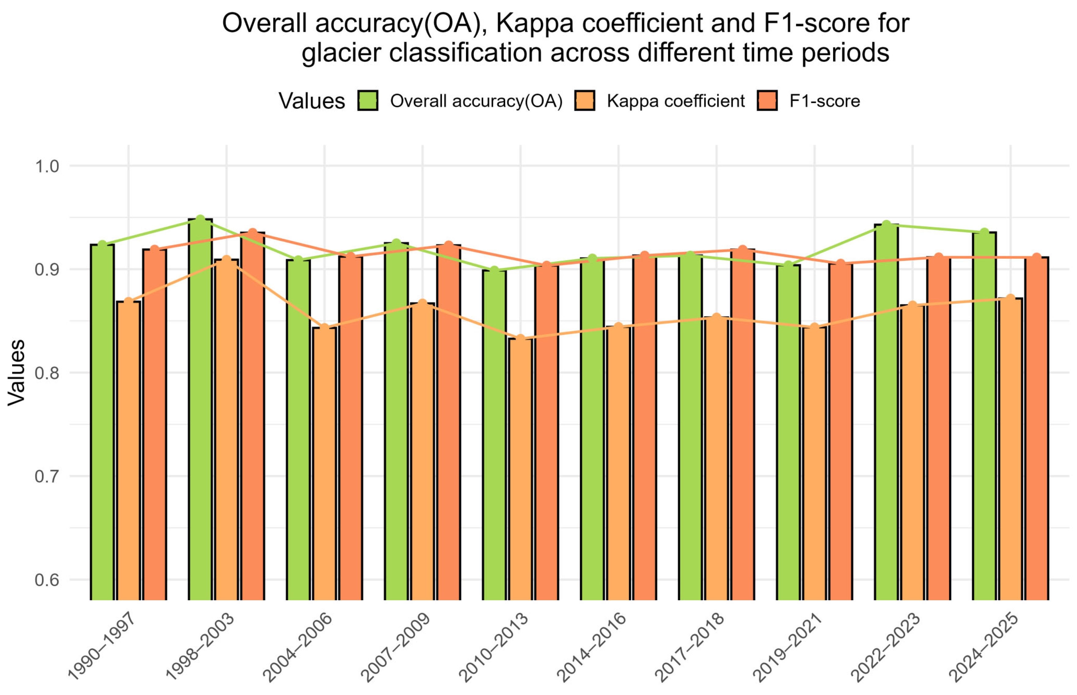
In this study, training and validation samples were randomly selected in a 7:3 ratio. Based on the validation data, this study calculated the OA, Kappa coefficient and F1-score for the classification results across each time period, as shown in Figure 6. The results indicated that the overall classification accuracy consistently remained above 90%, reaching a maximum of 95% (1998–2003 and 2022–2023). The Kappa coefficients were all higher than 0.83, and the highest was 0.91 (1998–2003). To further validate the accuracy of the model’s classification, the F1-score was included as a supplementary validation metric; all F1-scores exceeded 90%, further confirming the reliability of the classification method used in this study.

4.2. Comparison of Glacier Identification Results in Specific Areas

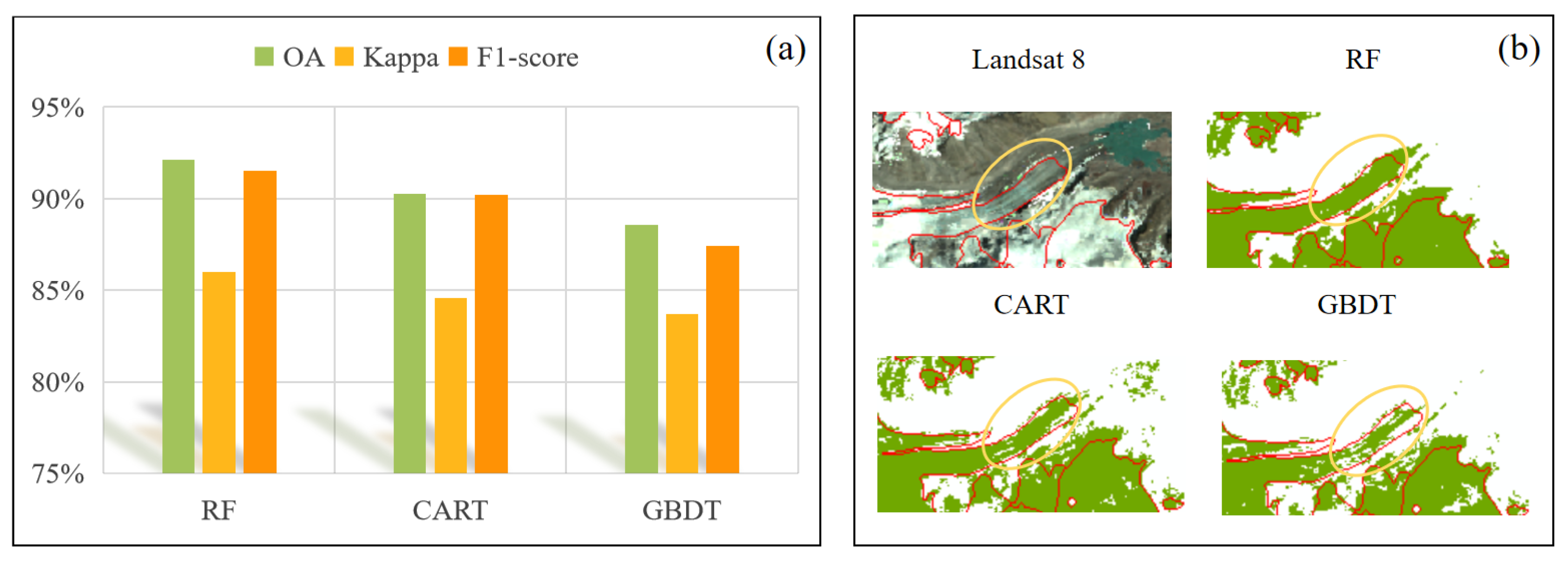
To further evaluate the recognition capabilities of different algorithms in complex terrain, we not only compared their quantitative accuracy (Figure 7a) but also conducted a qualitative assessment of their spatial recognition performance based on the 2017–2018 glacier inventory dataset for western China (Figure 7b). It is worth noting that the challenge in extracting glaciers via remote sensing lay not in clean glaciers. Whether using traditional band ratio methods or machine learning algorithms, clean glaciers could be extracted with high accuracy relatively easily due to their distinct spectral characteristics. However, for debris-covered glaciers, their surface spectral characteristics were highly similar to those of the surrounding bare rock and glacial debris, which lead conventional algorithms to frequently produce serious omission and misclassification errors. As shown by the yellow elliptical regions in Figure 7b, the glacier detection results from the RF algorithm were significantly better than those from the Classification and Regression Tree (CART) and the Gradient Boosting Decision Tree (GBDT). The detection accuracy of CART and GBDT for debris-covered glaciers still needed improvement, indicating that both algorithms had shortcomings in decoupling high-dimensional features and resisting noise. In contrast, the RF algorithm effectively overcame feature multicollinearity and mitigated the interference of outliers, thereby improving the accuracy of debris-covered glacier detection. This fully demonstrated that the multi-feature fusion RF framework offered the best robustness for debris-covered glacier detection.

4.3. Spatiotemporal Variation Characteristics of Tibetan Glaciers

4.3.1. Temporal Variations in Tibetan Glaciers

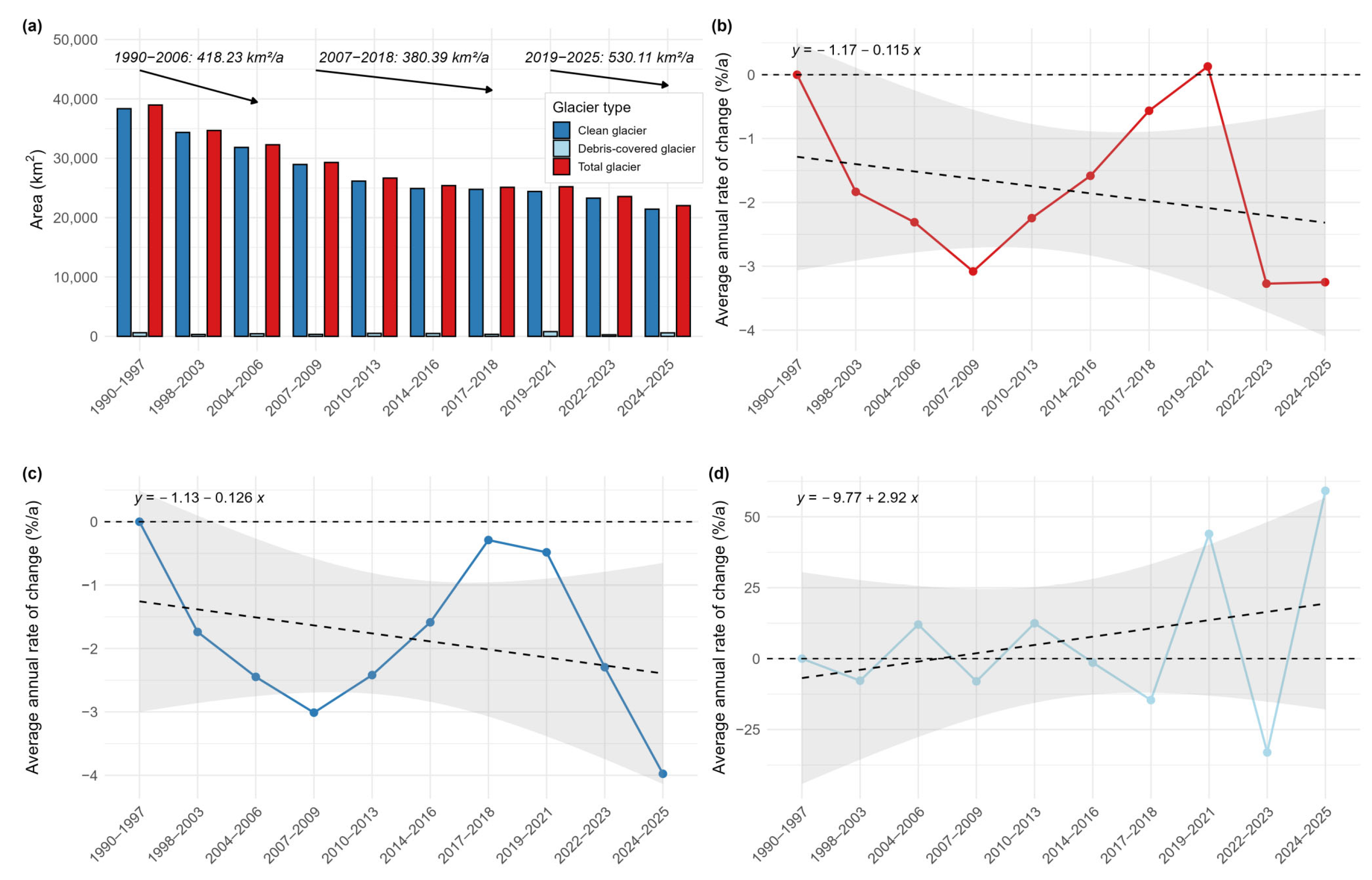
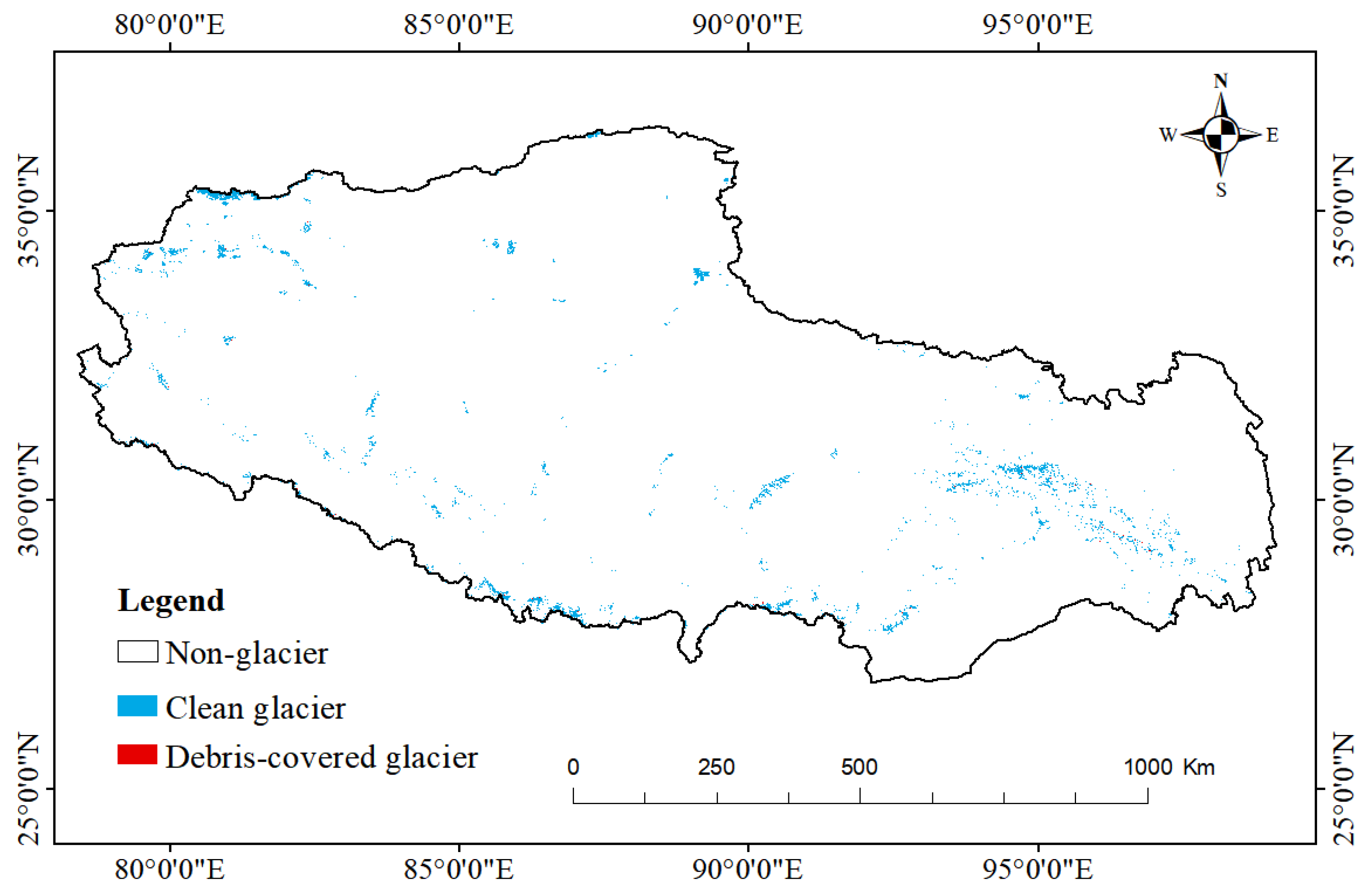
Based on long-term remote sensing image data, this study achieved high-precision extraction of glacier boundaries in Tibet from 1990 to 2025 and revealed the spatial distribution patterns and dynamic changes of glaciers in the region over the past 35 years. As shown in Figure 8, glaciers in Tibet generally exhibited a spatial distribution characterized by “sparse and scattered distribution in the west and high-density contiguous distribution in the east”. Among them, clean glaciers constituted the predominant type in Tibet, accounting for more than 95% of the total glacier area. During the 1990–2025 period, Tibetan glaciers exhibited a sustained overall retreat (Figure 9a). The total glacier area decreased from 38,968 km² in 1990–1997 to 22,026 km² in 2024–2025, representing a cumulative reduction of 16,942 km². The glacial retreat process exhibited significant variations across different phases: the average annual retreat area reached 418 km²/a from 1990 to 2006; from 2007 to 2018, the retreat rate temporarily slowed, with the average annual retreat area decreasing to 380 km²/a; however, from 2019 to 2025, the glacial retreat rate accelerated significantly again, with the average annual retreat area increasing to 530 km²/a. Further analysis of the annual average rate of area changes for different glacier types revealed (Figure 9b–d) that both total glaciers and clean glaciers exhibited a significant downward trend in their annual average rates of change, with annual retreat rates of 0.12%/a and 0.13%/a, respectively. This indicated that the retreat rate of clean glaciers was slightly higher than that of the total glaciers, making them the core factor driving the overall accelerated retreat of Tibetan glaciers. Conversely, unlike the continuous accelerated retreat of clean glaciers, the annual average rate of area changes for debris-covered glaciers displayed an upward trend, but the rate of change varied significantly across different time periods.

4.3.2. Spatial Variations in Tibetan Glaciers

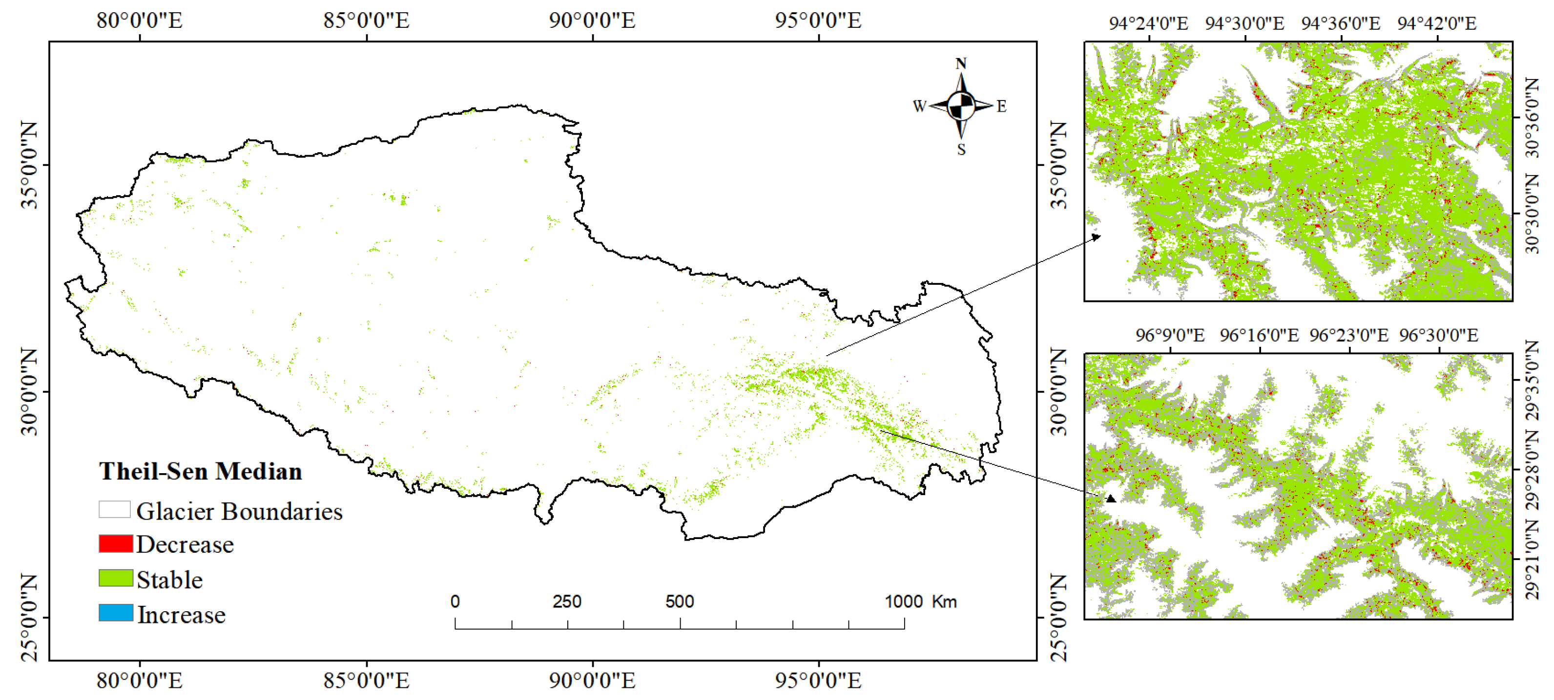
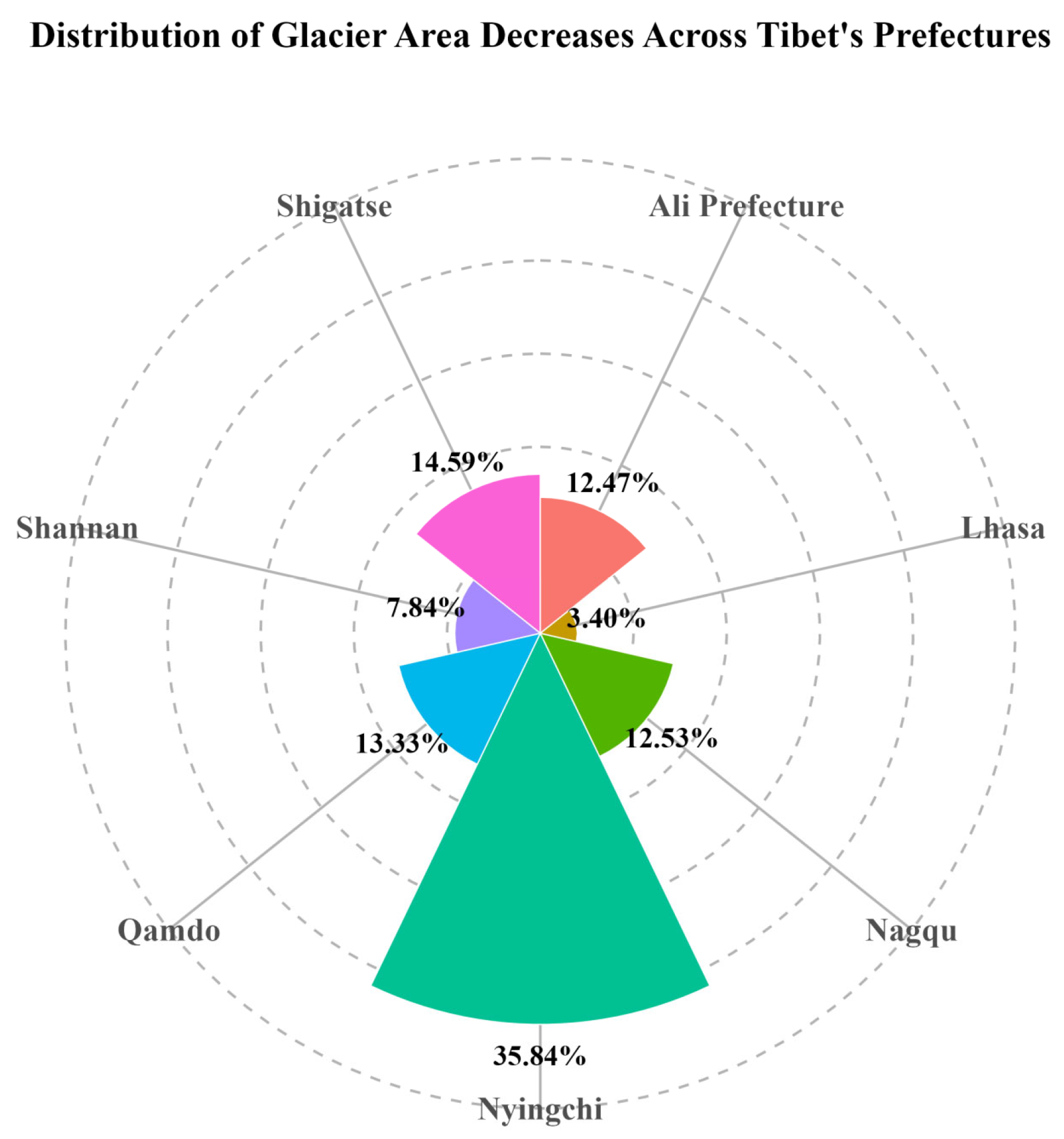
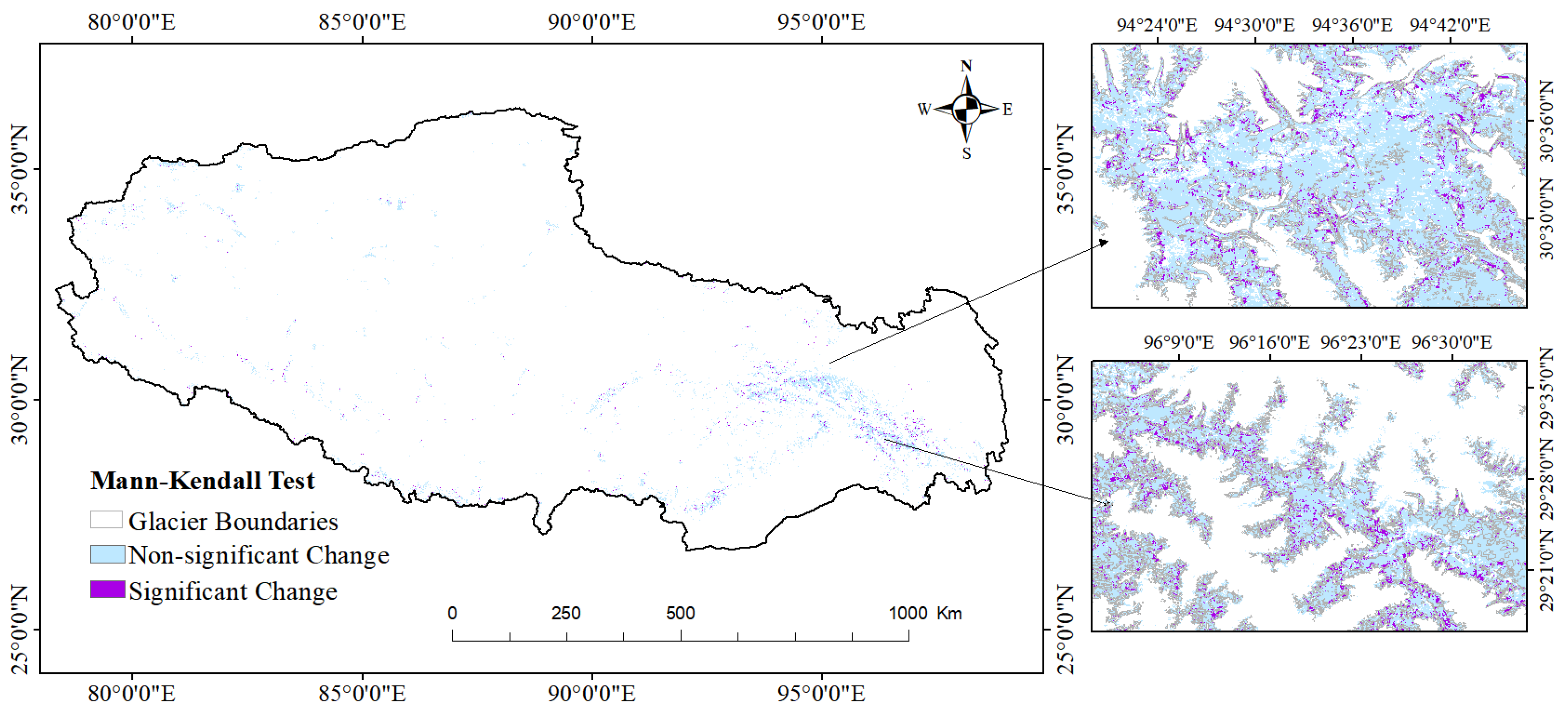
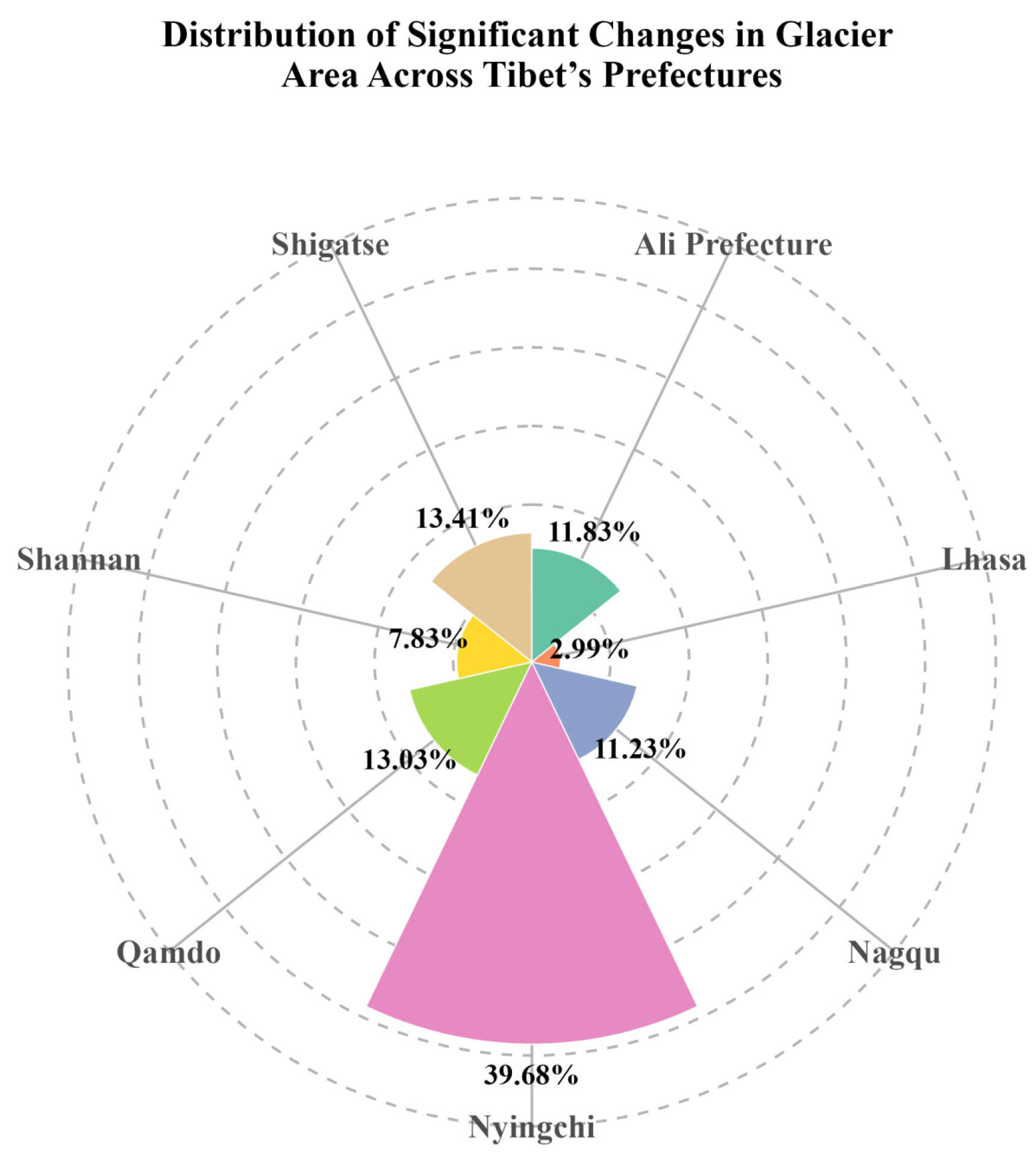
To further elucidate the spatial heterogeneity of glacial changes in Tibet, this study employed a combined approach of Theil–Sen median trend analysis and MK significance testing to analyze trends in glacial area changes in Tibet from 1990 to 2025. The results indicated that Tibetan glaciers generally showed a trend of continuous retreat, with the retreat primarily concentrated in the southeastern regions from 1990 to 2025 (Figure 10 and Figure 11), the combined glacial area retreat in Nyingchi and Shigatse cities accounted for 50.4% of the total retreat area. Furthermore, the results of the significance test of glacier area trends in Tibet from 1990 to 2025 (Figure 12 and Figure 13) showed that areas with significant changes in glacier area were mainly distributed in southeastern Tibet, which was highly consistent with the spatial distribution of area-decreasing units identified in the Theil–Sen trend analysis.

4.4. Characteristics of Glacial Changes at Different Elevations, Slopes and Aspects

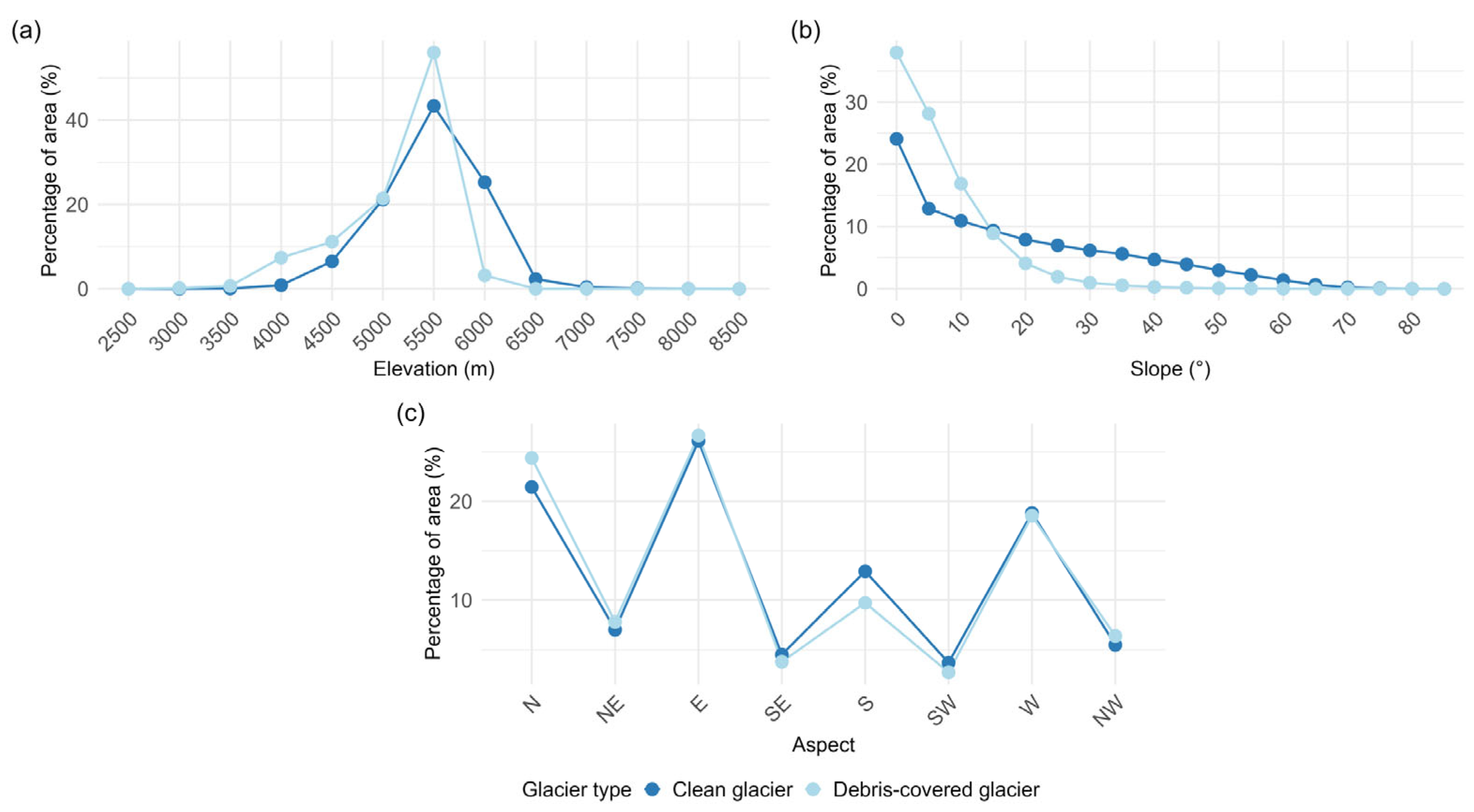
To provide a clear representation of glacier distributions across varying topographic gradients, this study analyzed glacier data from 2024–2025. In terms of elevation distribution (Figure 14a), the elevation distribution of glaciers in Tibet exhibited a distinct unimodal pattern, primarily concentrated in the mid-to-high elevation range of 4500–6500 m, which hosted over 90% of the total glacier area. The peak proportions of both clean and debris-covered glaciers occurred at 5500 m, at approximately 42% and 55%, respectively. This distribution pattern was closely related to the snowline elevation in Tibet. The 4500–6500 m range coincided with the equilibrium line elevation of most mountain ranges, where glacial accumulation and ablation were relatively balanced, favoring long-term glacial preservation. In terms of slope distribution (Figure 14b), the area of glaciers in Tibet decreased rapidly with increasing slope, and the distribution patterns of the two glacier types were highly consistent. Glaciers were primarily distributed in gentle terrain with slopes less than 20°, with the highest proportion of glacier area found in the 0–5° slope range: approximately 24% for clean glaciers and as high as 38% for debris-covered glaciers. When the slope exceeded 20°, the area proportions of both glacier types rapidly dropped to below 5%. In terms of aspect distribution (Figure 14c), Tibetan glaciers exhibited a distinct aspect preference, with east-facing (E) slopes showed the highest concentration of glaciers, the area proportions of clean and debris-covered glaciers on E slopes were approximately 26% and 27%, respectively. This was followed by north-facing (N) and west-facing (W) slopes, where clean glaciers accounted for approximately 22% and 19% of the area, respectively, while debris-covered glaciers accounted for approximately 25% and 18%, respectively. The proportion of glacier area on southwest-facing (SW) slopes was the lowest, at approximately 4%.

4.5. Characteristics of Glacial Changes in the Tibetan River Basins

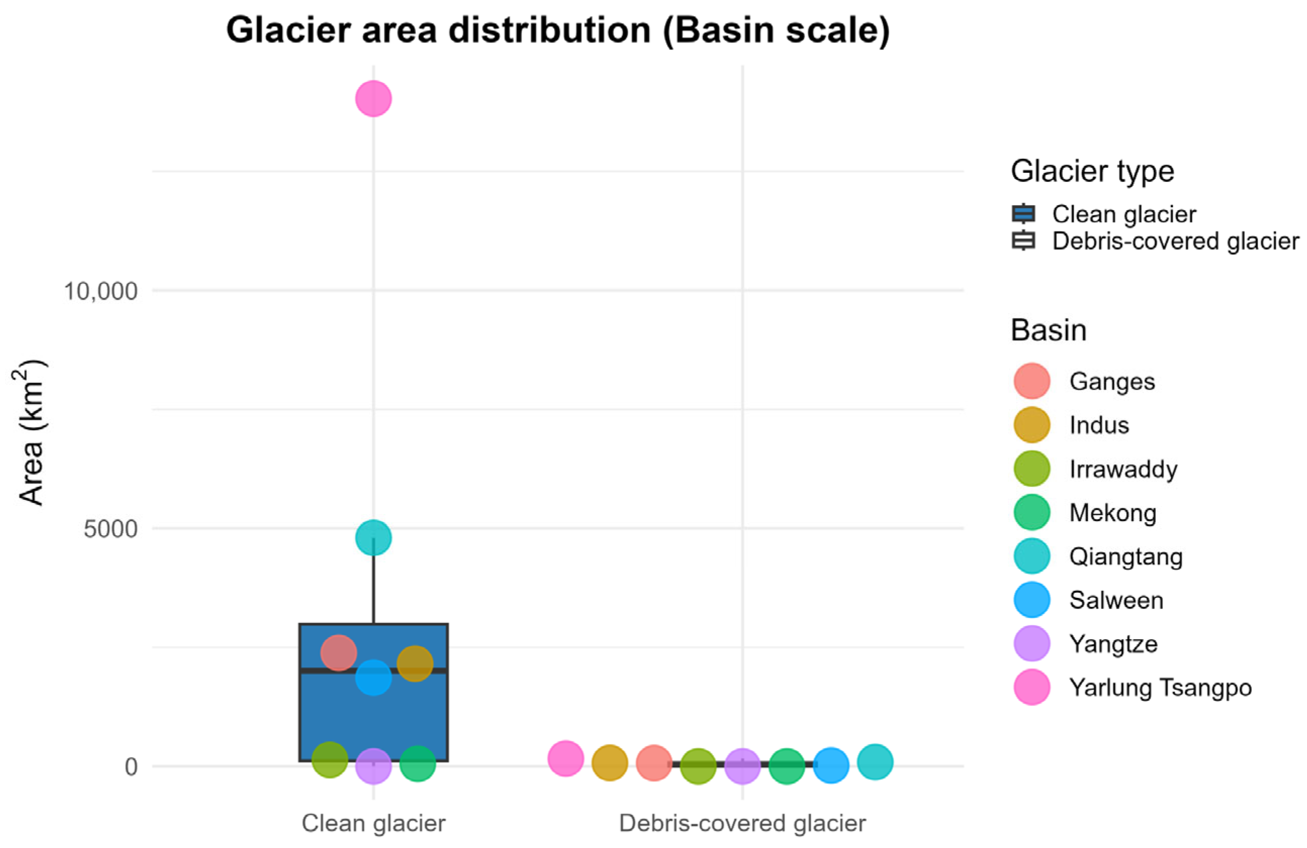
This study analyzed the distribution patterns and variations in retreat rates of glaciers in major Tibetan river basins from 1990 to 2025 at the watershed scale. Tibet’s glacial resources were primarily concentrated in a few select river basins (Figure 15). The Yarlung Tsangpo river basin accounted for the largest proportion of Tibetan glacial area, with clean and debris-covered glaciers comprising 55.18% and 39.82% of the total glacial area in Tibet, respectively. The Qiangtang river basin ranked second, with clean and debris-covered glaciers accounting for approximately 18.89% and 21.89% of the total glacial area in Tibet, respectively. The glacier areas in the remaining basins were relatively small; those in the Ganges, Salween, and Indus river basins ranged between 1000 and 3000 km², while those in the Mekong, Yangtze, and Irrawaddy river basins were all less than 1000 km².

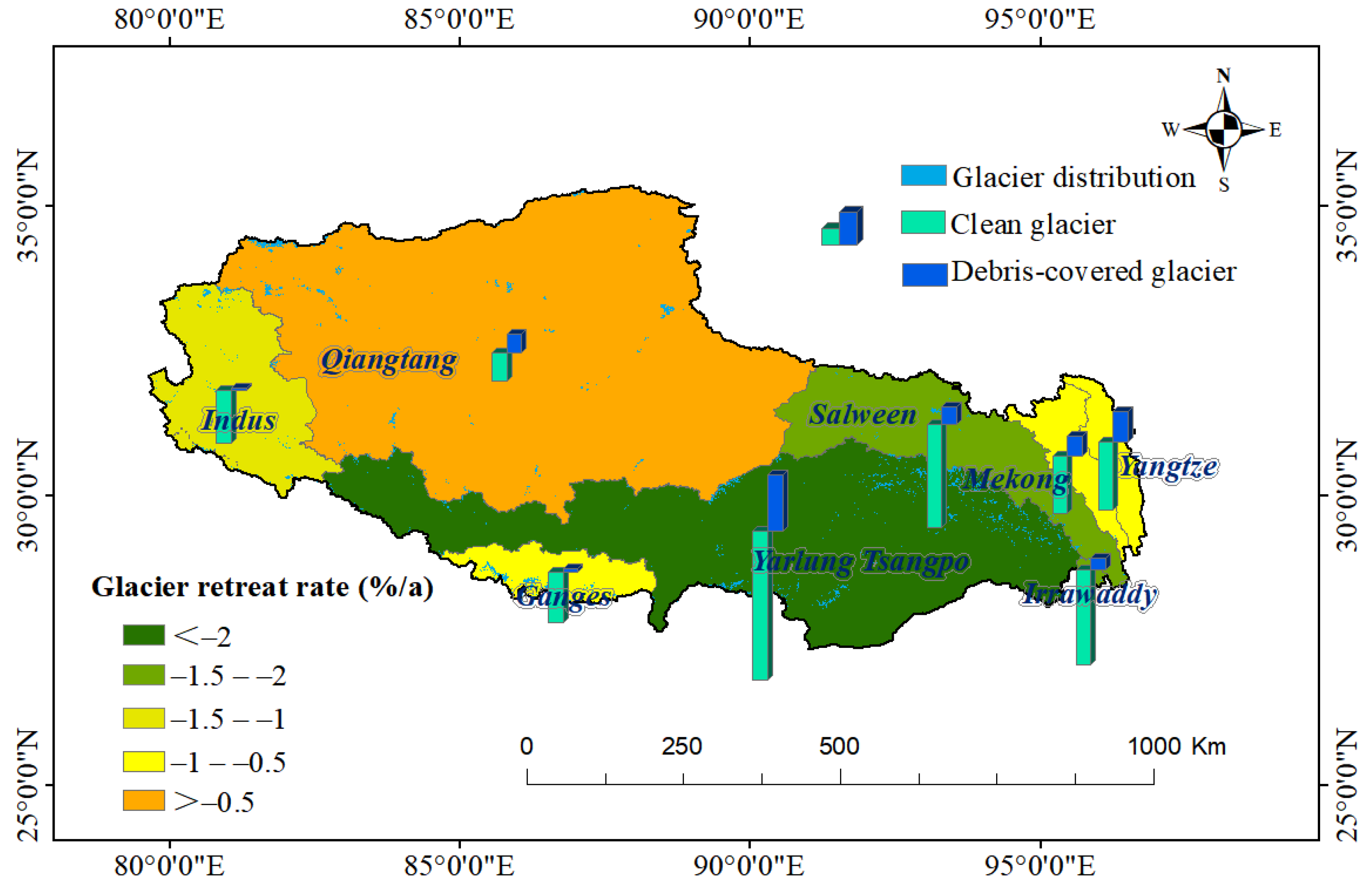
Results on the rates of glacier area change across different basins indicated that glaciers in all Tibetan basins exhibited a significant retreat trend from 1990 to 2025 (Figure 16). However, there were substantial differences in the average annual retreat rates among basins, with a general spatial pattern of faster retreat in the southeast and slower retreat in the northwest. Among these, the Yarlung Tsangpo river exhibited the fastest retreat rate, with an average annual decline exceeding 2%. Glaciers in southern river basins, such as the Irrawaddy and Salween, exhibited the second-fastest retreat rates, with annual average decline rates ranging between 1.5% and 2%. In contrast, glaciers in the inland Qiangtang basin retreated at the slowest rate, with annual average decline rates of only 0.1–0.5%, making it the region with the highest glacial stability in Tibet.

5. Discussion

5.1. Validation of Results Across Different Datasets

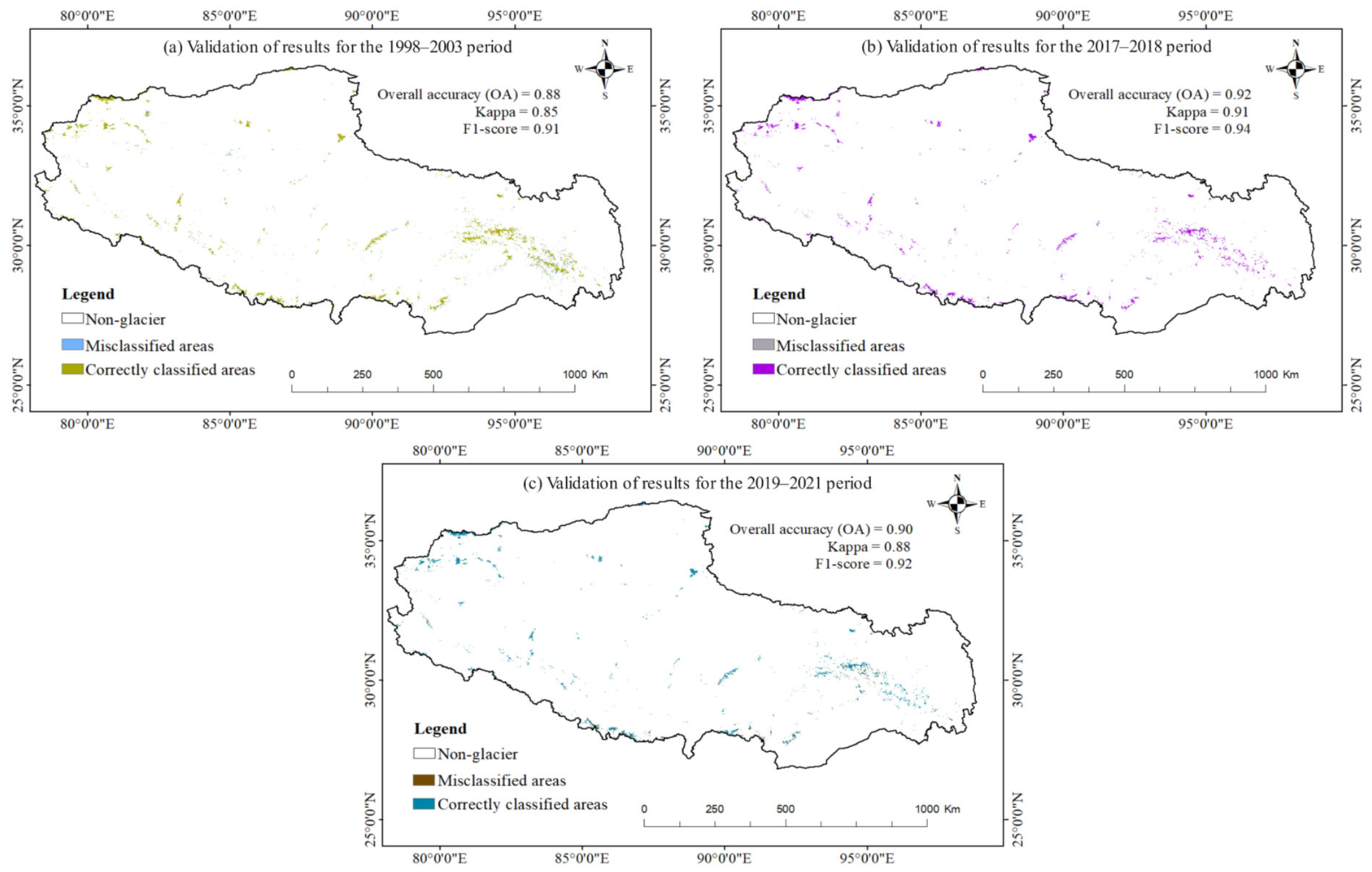
To objectively evaluate the accuracy of the Tibetan glacier grids extracted in this study, we used the Randolph Glacier Inventory (RGI 7.0), the 2017–2018 glacier inventory dataset for western China [36], and the 2020 glacier inventory dataset for High Mountain Asia [37] as validation datasets and calculated key evaluation metrics using the confusion matrix method. The quantitative evaluation results showed that the OA for the three time periods ranged from 0.88 to 0.92 (

Table 3. Validation of Glacier Detection Results.

Time Period	Data Validation Period	OA	Kappa	F1-Score
1998–2003	1996–2002	0.88	0.85	0.91
2017–2018	2017–2018	0.92	0.91	0.94
2019–2021	2020	0.90	0.88	0.92

), with the highest classification accuracy observed in the 2017–2018 period. Specifically, the Kappa coefficients fell within the “almost perfect” confidence interval [46], fully demonstrating the high spatial consistency between the extracted results and the validation data. Furthermore, the high F1-score further indicated that this method can effectively reduce misclassification in complex terrain such as glacier-rock mixed areas.

Combined with the spatial classification discrepancy map analysis (Figure 17), the correctly classified glacier areas for the 1998–2003, 2017–2018 and 2019–2021 periods were 29,325 km², 22,868 km² and 22,264 km², accounting for 84.56%, 91.08% and 88.33% of the total extracted glacier area, respectively. These correctly classified areas were primarily concentrated in major mountain ranges such as the Himalaya, Kunlun and Kaila Range, while misclassified areas were scattered in the mixed-pixel transition zones along glacier boundaries. Based on these quantitative and spatial statistical results, the dataset was confirmed to possess extremely high data reliability and completeness.

To further verify the accuracy of our extraction results, we compared them with the Second Chinese Glacier Inventory (CGI-2). Although CGI-2 utilized remote sensing imagery acquired between 2004 and 2011, its technical specifications stipulate that “when multiple high-quality images are available for a given glacier, the image closest in time to the inventory date shall be selected” [35]. Consequently, the resulting glacier outlines are effectively representative of conditions around 2010. The glacier area in Tibet recorded by CGI-2 is approximately 23,795.78 km², whereas our extraction for the 2010–2013 period yielded 26,662 km², which is notably higher. This discrepancy can be attributed to two main factors: first, the two datasets are not fully aligned in their temporal reference; second, systematic differences exist in extraction methods and classification criteria. CGI-2 employed a traditional semi-automatic approach combining band-ratio thresholding, morphological filtering, and manual visual revision, whereas this study used a Random Forest algorithm based on multi-feature fusion (spectral, textural, topographic features, and band differences). These two approaches differ in both glacier identification logic and boundary delineation standards, which objectively contribute to discrepancies in area statistics.

5.2. Phased Changes and Driving Mechanisms of Glacial Retreat in Tibet

The results of this study indicate that between 1990 and 2025, the area of glaciers in Tibet decreased by 43.5%, with the rate of retreat gradually accelerating. This long-term trend is closely related to the warming of the plateau against the backdrop of global warming [47]. In recent decades, the rate of surface warming on the Tibetan Plateau has been significantly higher than the global average for the same period; in particular, summer warming in high-altitude regions has directly driven the continued retreat and area reduction of glaciers [6]. Notably, the rate of glacial retreat between 2007 and 2018 slowed markedly compared to the period from 1990 to 2006. Considering that glacier area changes typically lag behind climate forcing by several years, this slowdown is understood as a delayed response to two favorable climatic factors. First, during the “global warming hiatus” of 1998–2012, the summer warming trend on the Plateau slowed or even stalled [48], directly reducing the energy input for glacial ablation and leading to a decrease in the regional glacial mass loss rate [49]. Second, annual precipitation on the plateau has increased significantly since 2000 [50], boosting mass replenishment and slowing the glacial retreat trend. Together, these two factors led to the deceleration in the retreat rate during this period.

Following this period of slowed retreat, glacier area did not immediately resume rapid retreat; instead, it increased briefly by 0.39% between 2019 and 2021. Analysis of changes in the areas of clean glaciers and debris-covered glaciers during this period revealed that the area of debris-covered glaciers increased, while clean glaciers continued to retreat. This indicates that intensified ablation accelerated the exposure of debris within the ice, while terminal collapses triggered by climate warming provided new debris, driving the transformation of clean glaciers into debris-covered glaciers [51,52]. In remote sensing interpretation, this increase in surface debris cover appeared as a temporary increase in “glacier area”; in essence, it was a signal of intense melting rather than a genuine improvement in mass balance. Starting in 2022, the rate of glacier retreat accelerated significantly, which may be related to the extreme heatwave that struck areas above 5000 m on the Tibetan Plateau in 2022 [53], where more than 80% of Tibet’s glaciers are located (Figure 14a). Extreme high temperatures caused a sharp increase in the ablation rates of snowpack and exposed ice surfaces, while simultaneously triggering a positive ice–albedo feedback (ablation darkens the ice surface, causing it to absorb more solar radiation), which further exacerbated mass loss and thus indirectly led to a significant acceleration in the rate of glacial retreat in Tibet starting in 2022.

Regarding glacier type responses, as the predominant glacier type in Tibet, the trend in the area of clean glaciers aligned with that of total glacier area, showing a continuous decline. In contrast, while debris-covered glaciers demonstrated an overall increasing trend, their rate of change was highly unstable across different time periods. The primary reason lies in the complex hydrology of debris-covered glaciers [54]. In addition to climatic impacts, factors such as the abundance of ice cliffs and glacial lakes also exert a significant influence on the melting rate of these debris-covered glaciers [55].

5.3. Regional Comparison and Methodological Differences in Glacier Retreat Rates

Due to significant topographic variations across the Tibetan Plateau, the spatial patterns of glacier area changes differ among regions [56,57]. Therefore, a systematic comparison of the results of this study with existing research can help to further elucidate trends in glacier retreat across different high-altitude regions.

At the regional scale, previous studies on glacial changes in southeastern Tibet, with results indicating that the total glacier area in that region decreased by 48.0% between 1970 and 2022 [58], whereas this study calculated a 35.3% decrease in the total glacier area of Tibet between 1990 and 2022. There are two main reasons for this discrepancy: first, the study by Wan covered a longer time period, resulting in greater cumulative glacier area retreat; second, that study area included only Nyingchi and Shannan prefectures in Tibet, which are the regions with the fastest glacier retreat rates in Tibet, thus yielding a greater percentage of area loss compared to this study.

At the Tibet-wide scale, a visual interpretation study based on RGI V7.0, CGI-2 data, and Landsat imagery, finding that the total glacier area in Tibet decreased by 14.75% from 2000 to 2022 [59], whereas this study reported a decrease of 27.32% over the same period. This discrepancy stems primarily from differences in remote sensing data selection strategies. Zhou et al. applied a 20% cloud cover threshold to mitigate interpretation errors caused by cloud cover. However, the Tibetan Plateau features complex topography, and some regions experience year-round cloud cover; strictly enforcing this threshold would result in the discarding of a large number of valid pixels, making it difficult to construct spatially continuous and complete imagery [14]. The resulting data gaps are particularly severe along glacier margins and termini, which directly introduce statistical errors in glacier area measurements and consequently lead to an underestimation of glacier area loss. In fact, the accuracy of glacier boundary interpretation significantly influences estimates of area change, with clouds, shadows, and classification methods all introducing errors [9].

Furthermore, across the Tibetan Plateau and surrounding regions, there are significant discrepancies in glacier area changes reported by different studies. For example, a study based on three independent methods (satellite gravimetry, laser altimetry, and glaciological modeling) showed that the rate of total glacier area retreat in the Tianshan Mountains between 1961 and 2012 ranged from 12 to 24% [60]; in the Himalayan region, the integration of multi-source satellite imagery and digital elevation models indicated a 31.03% reduction in glacier area from 1976 to 2024 [61]; in the Nyenchen Tanglha Mountains, a study based on Landsat and other remote sensing imagery combined with GIS technology showed that glacier area decreased by approximately 22% between 1972 and 2010, with the retreat rate accelerating significantly after 2000 [62]. In contrast, inland glaciers along the northern margin of the Tibetan Plateau retreated at a slower rate, with a retreat of 20.17% between 1990 and 2020 [63]. These comparisons indicate that the study period, spatial scope, data sources, and research methods are all key factors influencing estimates of retreat rates.

5.4. The Influence of Topographic Features on the Distribution of Glaciers in Tibet

The results indicated that the distribution of glaciers in Tibet was closely related to topographic factors such as elevation, slope, and aspect (Figure 14). In terms of elevation, glacier area exhibited a unimodal distribution, concentrated in the mid-to-high elevation range of 4500–6500 m, with a peak at approximately 5500 m. This elevation range largely corresponds to the snowline height on the Tibetan Plateau [64], where glacial accumulation and ablation are nearly in equilibrium, favoring glacial stability [6]. At elevations below 4500 m, temperatures are relatively high, leading to increased ablation; above 6500 m, the terrain is often steep and water vapor input is insufficient, limiting snow accumulation and hindering glacier development.

In terms of slope, glacier coverage decreased rapidly as slope steepness increased. When the slope was less than 15°, the area of debris-covered glaciers exceeded that of clean glaciers. This is because a thicker debris layer provides stronger thermal insulation, effectively reducing the glacier’s ablation rate and causing the slope to become gentler [65,66]. Furthermore, debris layer thickness is negatively correlated with slope; that is, the gentler the slope, the thicker the debris layer [67].

In terms of aspect, glacier distribution exhibited distinct directional differences. The E and N slopes accounted for the largest share, together comprising approximately 50% of the total glacier area, while the SW slope had the lowest proportion. This pattern is primarily governed by regional atmospheric circulation and local radiation regimes. As a windward slope, the E aspect intercepts the East Asian monsoon and part of the Indian monsoon, receiving abundant moisture conducive to glacial accumulation [68], which results in the largest glacial area. The N aspect is a shaded slope receiving approximately 15% less direct solar radiation during the glacial melt season [69], which effectively slows melting and makes it the second-largest glacier-bearing aspect. The W aspect, influenced by the mid-latitude westerlies, receives less moisture than the eastern slope but still benefits from moderate precipitation and some direct radiation during peak solar periods, ranking third in glacier area. Conversely, on the SW aspect, limited water vapor transport to the plateau leads to reduced precipitation [70], while intense solar radiation enhances heat flux and evaporation. These combined factors accelerate ablation and limit accumulation, resulting in the lowest glacier proportion on this aspect.

5.5. Characteristics of Glacial Changes at the Basin Scale

The results of this study indicated that the distribution of glacial resources in Tibet was highly uneven across different river basins, and there were significant differences in glacial retreat rates among these basins (Figure 15 and Figure 16). The Yarlung Tsangpo River basin was the region with the highest concentration of glacial resources in Tibet, primarily due to its close association with the moisture transport pathways of the Tibetan Plateau. As the main channel through which the Indian monsoon enters the Tibetan Plateau, the Yarlung Tsangpo River basin receives abundant precipitation [71]. Precipitation plays a dominant role in snowpack changes within the Yarlung Tsangpo River basin [72], making it the region with the highest concentration of glacial development. Regarding glacial retreat rates, glaciers in all basins exhibited a significant retreat trend between 1990 and 2025, but the rates of retreat varied considerably. The overall spatial pattern was characterized by “rapid retreat in the southeast and slow retreat in the northwest.” This spatial variation is primarily due to different atmospheric circulation systems governing each basin [6]. The southeastern basins are primarily influenced by the Indian monsoon, characterized by higher temperatures and highly seasonal precipitation. These glaciers are predominantly marine-type glaciers, which are extremely sensitive to temperature changes. In contrast, the northwestern Qiangtang basin is mainly controlled by the westerly circulation, featuring a cold and dry climate. The glaciers here are predominantly continental-type glaciers, with relatively low accumulation and ablation rates. This results in weaker glacial activity and a higher energy threshold required for ablation, leading to a slower retreat [4].

5.6. Limitations and Future Directions

Although this study achieved high-precision extraction of glacier changes in Tibet based on long-term remote sensing data and established a glacier dataset for the period 1990–2025, the following limitations remain and require further improvement in future research.

First, there is an inherent inconsistency between area changes and volume changes. This study primarily relied on two-dimensional glacier boundaries to extract area changes and was unable to directly quantify losses in glacier thickness and volume. Area retreat typically lags behind volume loss, particularly in thick ice regions. Future studies should combine remote sensing observations (such as high-resolution DEMs, ICESat-2, and GRACE satellite data) with field monitoring (such as ice radar thickness measurements and pole-based mass balance observations) to develop empirical or physical models for estimating volume changes, thereby more accurately reflecting the glacier’s mass balance.

Second, this study was limited by single-source remote sensing observations and the lack of an integrated framework. In the future, an integrated “remote sensing–field measurements–modeling” framework should be established: (1) use remote sensing data to provide a macro-level context of glacier distribution (spatiotemporal trends); (2) use field monitoring data (e.g., automatic weather stations, mass balance poles, ice radar) to provide localized calibration of key parameters; (3) employ numerical models (e.g., glacier dynamics models or energy balance models) for mechanism simulation and future scenario projections. Through cross-validation of multi-source data, we can further enhance our understanding of the mechanisms underlying glacier changes and their hydrological effects.

Third, the glacier boundaries in this study were extracted through automatic classification based on machine learning algorithms. Although the overall classification accuracy for all 10 time periods exceeded 90%, factors such as mixed pixels in high-altitude areas, topographic shading, residual seasonal snow, and spectral confusion in areas covered by glacial debris can lead to misclassification or omission errors during the classification process. These errors may indirectly affect the final glacier area statistics. Therefore, all area values in this study have been rounded to better account for the inherent uncertainty in remote sensing classification. Consequently, in future research, multi-source high-resolution validation data will be combined with error propagation models to further quantify the uncertainty range of the estimated area changes.

6. Conclusions

Based on the GEE platform and the RF algorithm, this study systematically analyzed the spatiotemporal variation characteristics of glaciers in Tibet from 1990 to 2025. The results indicated that over the past 35 years, glaciers in Tibet have exhibited a continuous retreat trend, with the total glacier area decreasing from 38,968 km² to 22,026 km², representing a cumulative reduction of 16,942 km². The retreat rate exhibited distinct phases; the “global warming hiatus” and increased precipitation jointly led to a deceleration in glacial retreat during 2007–2018 relative to 1990–2006. In terms of topographic characteristics, Tibetan glaciers were most concentrated at an elevation of 5500 m and on E aspect. Spatially, the Yarlung Tsangpo River basin experienced the fastest retreat (>2%/a), whereas the Qiangtang basin showed the highest stability (0.1–0.5%/a), primarily controlled by different atmospheric circulation systems. This study demonstrated that the proposed remote sensing indicators coupled with the RF algorithm provided an effective tool for large-scale, long-term glacier monitoring. The findings offered important data support for understanding glacier responses to climate change and assessing water resource security in the Tibetan Plateau region.

References

1. Cogley, J.G.; Hock, R.; Rasmussen, L.A.; Arendt, A.A.; Bauder, A.; Braithwaite, R.J.; Jansson, P.; Kaser, G.; Möller, M.; Nicholson, L.; et al. Glossary of Glacier Mass Balance and Related Terms; IHP-VII Technical Documents in Hydrology No. 86; IACS Contribution No. 2; UNESCO-IHP: Paris, France, 2011. [Google Scholar]
2. Bojinski, S.; Verstraete, M.; Peterson, T.C.; Richter, C.; Simmons, A.; Zemp, M. The Concept of Essential Climate Variables in Support of Climate Research, Applications, and Policy. Bull. Am. Meteorol. Soc. 2014, 95, 1431–1443. [Google Scholar] [CrossRef] [Scilit]
3. Liu, X.; Chen, B. Climatic warming in the Tibetan Plateau during recent decades. Int. J. Climatol. 2000, 20, 1729–1742. [Google Scholar]
4. Brun, F.; Berthier, E.; Wagnon, P.; Kääb, A.; Treichler, D. A spatially resolved estimate of High Mountain Asia glacier mass balances from 2000 to 2016. Nat. Geosci. 2017, 10, 668–673. [Google Scholar] [CrossRef] [Scilit] [PubMed]
5. Xiao, C.-D.; Wang, S.-J.; Qin, D.-H. A preliminary study of cryosphere service function and value evaluation. Adv. Clim. Change Res. 2015, 6, 181–187. [Google Scholar] [CrossRef] [Scilit]
6. Yao, T.; Thompson, L.; Yang, W.; Yu, W.; Gao, Y.; Guo, X.; Yang, X.; Duan, K.; Zhao, H.; Xu, B.; et al. Different glacier status with atmospheric circulations in Tibetan Plateau and surroundings. Nat. Clim. Change 2012, 2, 663–667. [Google Scholar] [CrossRef] [Scilit]
7. Millan, R.; Mouginot, J.; Rabatel, A.; Morlighem, M. Ice velocity and thickness of the world’s glaciers. Nat. Geosci. 2022, 15, 124–129. [Google Scholar] [CrossRef] [Scilit]
8. Zemp, M.; Huss, M.; Thibert, E.; Eckert, N.; McNabb, R.; Huber, J.; Barandun, M.; Machguth, H.; Nussbaumer, S.U.; Gärtner-Roer, I.; et al. Global glacier mass changes and their contributions to sea-level rise from 1961 to 2016. Nature 2019, 568, 382–386. [Google Scholar] [CrossRef] [Scilit] [PubMed]
9. Paul, F.; Barrand, N.E.; Baumann, S.; Berthier, E.; Bolch, T.; Casey, K.; Frey, H.; Joshi, S.P.; Konovalov, V.; Le Bris, R.; et al. On the accuracy of glacier outlines derived from remote-sensing data. Ann. Glaciol. 2013, 54, 171–182. [Google Scholar] [CrossRef] [Scilit]
10. Kulkarni, A.; Srinivasulu, J.; Manjul, S.; Mathur, P. Field based spectral reflectance studies to develop NDSI method for snow cover monitoring. J. Indian Soc. Remote Sens. 2002, 30, 73–80. [Google Scholar] [CrossRef] [Scilit]
11. Zhang, M.; Wang, X.; Shi, C.; Yan, D. Automated Glacier Extraction Index by Optimization of Red/SWIR and NIR/SWIR Ratio Index for Glacier Mapping Using Landsat Imagery. Water 2019, 11, 1223. [Google Scholar] [CrossRef] [Scilit]
12. Walter, V. Object-based classification of remote sensing data for change detection. ISPRS J. Photogramm. Remote Sens. 2004, 58, 225–238. [Google Scholar] [CrossRef] [Scilit]
13. Huang, L.; Li, Z.; Tian, B.-S.; Chen, Q.; Liu, J.-L.; Zhang, R. Classification and snow line detection for glacial areas using the polarimetric SAR image. Remote Sens. Environ. 2011, 115, 1721–1732. [Google Scholar] [CrossRef] [Scilit]
14. Hu, M.; Zhou, G.; Lv, X.; Zhou, L.; He, X.; Tian, Z. A New Automatic Extraction Method for Glaciers on the Tibetan Plateau under Clouds, Shadows and Snow Cover. Remote Sens. 2022, 14, 3084. [Google Scholar] [CrossRef] [Scilit]
15. Robson, B.A.; Nuth, C.; Dahl, S.O.; Hölbling, D.; Strozzi, T.; Nielsen, P.R. Automated classification of debris-covered glaciers combining optical, SAR and topographic data in an object-based environment. Remote Sens. Environ. 2015, 170, 372–387. [Google Scholar] [CrossRef] [Scilit]
16. Xie, Z.; Haritashya, U.K.; Asari, V.K.; Young, B.W.; Bishop, M.P.; Kargel, J.S. GlacierNet: A Deep-Learning Approach for Debris-Covered Glacier Mapping. IEEE Access 2020, 8, 83495–83510. [Google Scholar] [CrossRef] [Scilit]
17. Holobâcă, I.-H.; Tielidze, L.G.; Ivan, K.; Elizbarashvili, M.; Alexe, M.; Germain, D.; Petrescu, S.H.; Pop, O.T.; Gaprindashvili, G. Multi-sensor remote sensing to map glacier debris cover in the Greater Caucasus, Georgia. J. Glaciol. 2021, 67, 685–696. [Google Scholar] [CrossRef] [Scilit]
18. Khan, A.A.; Jamil, A.; Hussain, D.; Taj, M.; Jabeen, G.; Malik, M.K. Machine-Learning Algorithms for Mapping Debris-Covered Glaciers: The Hunza Basin Case Study. IEEE Access 2020, 8, 12725–12734. [Google Scholar] [CrossRef] [Scilit]
19. Yang, S.; Wang, F.; Xie, Y.; Zhao, W.; Bai, C.; Liu, J.; Xu, C. Delineation Evaluation and Variation of Debris-Covered Glaciers Based on the Multi-Source Remote Sensing Images, Take Glaciers in the Eastern Tomur Peak Region for Example. Remote Sens. 2023, 15, 2575. [Google Scholar] [CrossRef] [Scilit]
20. Racoviteanu, A.; Williams, M.W. Decision Tree and Texture Analysis for Mapping Debris-Covered Glaciers in the Kangchenjunga Area, Eastern Himalaya. Remote Sens. 2012, 4, 3078–3109. [Google Scholar] [CrossRef] [Scilit]
21. Gorelick, N.; Hancher, M.; Dixon, M.; Ilyushchenko, S.; Thau, D.; Moore, R. Google Earth Engine: Planetary-scale geospatial analysis for everyone. Remote Sens. Environ. 2017, 202, 18–27. [Google Scholar] [CrossRef] [Scilit]
22. Hird, J.N.; Kariyeva, J.; McDermid, G.J. Satellite Time Series and Google Earth Engine Democratize the Process of Forest-Recovery Monitoring over Large Areas. Remote Sens. 2021, 13, 4745. [Google Scholar] [CrossRef] [Scilit]
23. Zhao, Q.; Yu, L.; Li, X.; Peng, D.; Zhang, Y.; Gong, P. Progress and Trends in the Application of Google Earth and Google Earth Engine. Remote Sens. 2021, 13, 3778. [Google Scholar] [CrossRef] [Scilit]
24. Amani, M.; Mahdavi, S.; Afshar, M.; Brisco, B.; Huang, W.; Mohammad Javad Mirzadeh, S.; White, L.; Banks, S.; Montgomery, J.; Hopkinson, C. Canadian Wetland Inventory using Google Earth Engine: The First Map and Preliminary Results. Remote Sens. 2019, 11, 842. [Google Scholar] [CrossRef] [Scilit]
25. Sazib, N.; Mladenova, I.; Bolten, J. Leveraging the Google Earth Engine for Drought Assessment Using Global Soil Moisture Data. Remote Sens. 2018, 10, 1265. [Google Scholar] [CrossRef] [Scilit] [PubMed]
26. Hu, Y.; Hu, Y. Land Cover Changes and Their Driving Mechanisms in Central Asia from 2001 to 2017 Supported by Google Earth Engine. Remote Sens. 2019, 11, 554. [Google Scholar] [CrossRef] [Scilit]
27. Tong, S.; Dong, Z.; Zhang, J.; Bao, Y.; Guna, A.; Bao, Y. Spatiotemporal Variations of Land Use/Cover Changes in Inner Mongolia (China) during 1980–2015. Sustainability 2018, 10, 4730. [Google Scholar] [CrossRef] [Scilit]
28. Deng, Y.; Jiang, W.; Tang, Z.; Ling, Z.; Wu, Z. Long-Term Changes of Open-Surface Water Bodies in the Yangtze River Basin Based on the Google Earth Engine Cloud Platform. Remote Sens. 2019, 11, 2213. [Google Scholar] [CrossRef] [Scilit]
29. Mahdianpari, M.; Salehi, B.; Mohammadimanesh, F.; Homayouni, S.; Gill, E. The First Wetland Inventory Map of Newfoundland at a Spatial Resolution of 10 m Using Sentinel-1 and Sentinel-2 Data on the Google Earth Engine Cloud Computing Platform. Remote Sens. 2019, 11, 43. [Google Scholar] [CrossRef] [Scilit]
30. Vale, A.B.; Arnold, N.S.; Rees, W.G.; Lea, J.M. Remote Detection of Surge-Related Glacier Terminus Change across High Mountain Asia. Remote Sens. 2021, 13, 1309. [Google Scholar] [CrossRef] [Scilit]
31. Xie, F.; Liu, S.; Wu, K.; Zhu, Y.; Gao, Y.; Qi, M.; Duan, S.; Saifullah, M.; Tahir, A.A. Upward Expansion of Supra-Glacial Debris Cover in the Hunza Valley, Karakoram, During 1990~2019. Front. Earth Sci. 2020, 8, 308. [Google Scholar] [CrossRef] [Scilit]
32. Zhang, J.; Jia, L.; Menenti, M.; Zhou, J.; Ren, S. Glacier Area and Snow Cover Changes in the Range System Surrounding Tarim from 2000 to 2020 Using Google Earth Engine. Remote Sens. 2021, 13, 5117. [Google Scholar] [CrossRef] [Scilit]
33. Huang, L.; Li, Z.; Zhou, J.M.; Zhang, P. An automatic method for clean glacier and nonseasonal snow area change estimation in High Mountain Asia from 1990 to 2018. Remote Sens. Environ. 2021, 258, 112376. [Google Scholar] [CrossRef] [Scilit]
34. Bevington, A.R.; Menounos, B. Accelerated change in the glaciated environments of western Canada revealed through trend analysis of optical satellite imagery. Remote Sens. Environ. 2022, 270, 112862. [Google Scholar] [CrossRef] [Scilit]
35. Liu, S.Y.; Yao, X.J.; Guo, W.Q.; Xu, J.L.; Shangguan, D.H.; Wei, J.F.; Bao, W.J.; Wu, L.Z. The present status of glaciers in China based on the Second Chinese Glacier Inventory. Acta Geogr. Sin. 2015, 70, 3–16. (In Chinese) [Google Scholar] [CrossRef]
36. Ran, W.; Wang, X.; Guo, W.; Zhao, H.; Zhao, X.; Liu, S.; Wei, J.; Zhang, Y. A Dataset of Glacier Inventory in Western China During 2017–2018 (V1); Science Data Bank: Beijing, China, 2021. [Google Scholar]
37. Ke, C.; Xiao, Y.; Fan, Y.; Luo, L.; Cai, Y.; Shen, X.; Wang, G.; Wu, J.; Zhuang, L.; Wang, J.; et al. A new time-stamped glacier inventory of High Mountain Asia based on deep learning and remote sensing big data in 2020. Sci. China Earth Sci. 2025, 69, 236–252. [Google Scholar] [CrossRef] [Scilit]
38. He, D.; Wang, L. Texture features based on texture spectrum. Pattern Recogn. 1991, 24, 391–399. [Google Scholar] [CrossRef] [Scilit]
39. Haralick, R.M.; Shanmugam, K.; Dinstein, I. Textural Features for Image Classification. IEEE Trans. Syst. Man Cybern. 1973, 3, 610–619. [Google Scholar] [CrossRef] [Scilit]
40. Breiman, L. Random Forests. Mach. Learn. 2001, 45, 5–32. [Google Scholar] [CrossRef] [Scilit]
41. Gislason, P.O.; Benediktsson, J.A.; Sveinsson, J.R. Random Forests for land cover classification. Pattern Recogn. Lett. 2006, 27, 294–300. [Google Scholar] [CrossRef] [Scilit]
42. Pal, M. Random forest classifier for remote sensing classification. Int. J. Remote Sens. 2005, 26, 217–222. [Google Scholar] [CrossRef] [Scilit]
43. Huang, X.; Lu, Q.; Zhang, L.; Antonio, P. New Postprocessing Methods for Remote Sensing Image Classification: A Systematic Study. IEEE Trans. Geosci. Remote Sens. 2014, 52, 7140–7159. [Google Scholar] [CrossRef] [Scilit]
44. Lunetta, R.S.; Knight, J.F.; Ediriwickrema, J.; Lyon, J.G.; Worthy, L.D. Land-cover change detection using multi-temporal MODIS NDVI data. Remote Sens. Environ. 2006, 105, 142–154. [Google Scholar] [CrossRef] [Scilit]
45. Milich, L.; Weiss, E. GAC NDVI interannual coefficient of variation (CoV) images: Ground truth sampling of the Sahel along north-south transects. Int. J. Remote Sens. 2000, 21, 235–260. [Google Scholar] [CrossRef] [Scilit]
46. Foody, G.M. Explaining the unsuitability of the kappa coefficient in the assessment and comparison of the accuracy of thematic maps obtained by image classification. Remote Sens. Environ. 2020, 239, 111630. [Google Scholar] [CrossRef] [Scilit]
47. He, M.; Li, Z.; Jiang, W.; Pan, Y.; Jiao, J.; Xiao, Y. Seasonal and Interannual Fluctuations of Glacier Mass Balance and Climate Response Processes on the Tibetan Plateau Based on GRACE/GRACE-FO. IEEE Trans. Geosci. Remote Sens. 2023, 61, 4301709. [Google Scholar] [CrossRef] [Scilit]
48. Medhaug, I.; Stolpe, M.B.; Fischer, E.M.; Knutti, R. Reconciling controversies about the ‘global warming hiatus’. Nature 2017, 545, 41–47. [Google Scholar] [CrossRef] [Scilit] [PubMed]
49. Zhu, M.; Wang, S.; Gao, X.; Bai, S.; Zhang, F.; Zhu, F.; Zhao, H. Reduced glacier mass loss rates on the southern Tibetan Plateau during a global warming hiatus. Glob. Planet. Change 2026, 262, 105476. [Google Scholar] [CrossRef] [Scilit]
50. Kuang, X.; Jiao, J.J. Review on climate change on the Tibetan Plateau during the last half century. J. Geophys. Res. Atmos. 2016, 121, 3979–4007. [Google Scholar] [CrossRef] [Scilit]
51. Benn, D.I.; Bolch, T.; Hands, K.; Gulley, J.; Luckman, A.; Nicholson, L.I.; Quincey, D.; Thompson, S.; Toumi, R.; Wiseman, S. Response of debris-covered glaciers in the Mount Everest region to recent warming, and implications for outburst flood hazards. Earth-Sci. Rev. 2012, 114, 156–174. [Google Scholar] [CrossRef] [Scilit]
52. Scherler, D.; Bookhagen, B.; Strecker, M.R. Spatially variable response of Himalayan glaciers to climate change affected by debris cover. Nat. Geosci. 2011, 4, 156–159. [Google Scholar] [CrossRef] [Scilit]
53. Gui, K.; Zhou, T.; Zhang, W.; Zhang, X. Land-atmosphere coupling amplified the record-breaking heatwave at altitudes above 5000 m on the Tibetan Plateau in July 2022. Weather Clim. Extrem. 2024, 45, 100717. [Google Scholar] [CrossRef] [Scilit]
54. Miles, K.E.; Hubbard, B.; Irvine-Fynn, T.D.L.; Miles, E.S.; Quincey, D.J.; Rowan, A.V. Hydrology of debris-covered glaciers in High Mountain Asia. Earth-Sci. Rev. 2020, 207, 103212. [Google Scholar] [CrossRef] [Scilit]
55. Huang, L.; Li, Z.; Han, H.; Tian, B.; Zhou, J. Analysis of thickness changes and the associated driving factors on a debris-covered glacier in the Tienshan Mountain. Remote Sens. Environ. 2018, 206, 63–71. [Google Scholar] [CrossRef] [Scilit]
56. Patel, L.K.; Sharma, P.; Fathima, T.N.; Thamban, M. Geospatial observations of topographical control over the glacier retreat, Miyar basin, Western Himalaya, India. Environ. Earth Sci. 2018, 77, 190. [Google Scholar] [CrossRef] [Scilit]
57. Yao, T.; Yu, W.; Wu, G.; Xu, B.; Yang, W.; Zhao, H.; Wang, W.; Li, S.; Wang, N.; Li, Z.; et al. Glacier anomalies and relevant disaster risks on the Tibetan Plateau and surroundings. Chin. Sci. Bull. 2019, 64, 2770–2782. (In Chinese) [Google Scholar] [CrossRef] [Scilit]
58. Wan, Q. Spatiotemporal Variation Characteristics and Driving Forces of Glaciers in Southeastern Xizang over the Past 50 Years. Master’s Thesis, Chengdu University of Technology, Chengdu, China, 2024. [Google Scholar]
59. Zhou, S.; Wang, N.; Li, Z.; Chang, J.; Zhang, Y.; Yao, X. Spatiotemporal characteristics of glacier area and length changes in Xizang, China, from 2000 to 2022. Int. J. Digit. Earth. 2025, 18, 2513046. [Google Scholar] [CrossRef] [Scilit]
60. Farinotti, D.; Longuevergne, L.; Moholdt, G.; Duethmann, D.; Mölg, T.; Bolch, T.; Vorogushyn, S.; Güntner, A. Substantial glacier mass loss in the Tien Shan over the past 50 years. Nat. Geosci. 2015, 8, 716–722. [Google Scholar] [CrossRef] [Scilit]
61. Thongley, T.; Tielidze, L.G.; Yang, W.; Gunn, A.; Mackintosh, A.N. Accelerated Glacier Area Loss and Extinction of Small Glaciers in the Bhutanese Himalaya over the Past Five Decades. Remote Sens. 2026, 18, 323. [Google Scholar] [CrossRef] [Scilit]
62. Wang, X.; Siegert, F.; Zhou, A.-g.; Franke, J. Glacier and glacial lake changes and their relationship in the context of climate change, Central Tibetan Plateau 1972–2010. Glob. Planet. Change 2013, 111, 246–257. [Google Scholar] [CrossRef] [Scilit]
63. Fang, C.; Zhu, R.; Yin, Z.; Chen, Z.; Shan, J.; Wang, L.; Yang, H. Remote sensing monitoring of glacier area and volume changes in glacier-fed mountainous watershed on the Northern margin of the Tibetan Plateau under climate change. Environ. Monit. Assess. 2024, 196, 966. [Google Scholar] [CrossRef] [Scilit] [PubMed]
64. Ye, W.; Wang, F.; Li, Z.; Zhang, H.; Xu, C.; Huai, B. Temporal and spatial distributions of the equilibrium line altitudes of the monitoring glaciers in High Asia. J. Glaciol. Geocryol. 2016, 38, 1459–1469. (In Chinese) [Google Scholar] [CrossRef]
65. Boxall, K.; Willis, I.; Giese, A.; Liu, Q. Quantifying Patterns of Supraglacial Debris Thickness and Their Glaciological Controls in High Mountain Asia. Front. Earth Sci. 2021, 9, 657440. [Google Scholar] [CrossRef] [Scilit]
66. Salerno, F.; Thakuri, S.; Tartari, G.; Nuimura, T.; Sunako, S.; Sakai, A.; Fujita, K. Debris-covered glacier anomaly? Morphological factors controlling changes in the mass balance, surface area, terminus position, and snow line altitude of Himalayan glaciers. Earth Planet. Sci. Lett. 2017, 471, 19–31. [Google Scholar] [CrossRef] [Scilit]
67. Pratap, B.; Sharma, P.; Patel, L.K.; Singh, A.T.; Oulkar, S.N.; Thamban, M. Differential surface melting of a debris-covered glacier and its geomorphological control—A case study from Batal Glacier, western Himalaya. Geomorphology 2023, 431, 108686. [Google Scholar] [CrossRef] [Scilit]
68. Seok, S.-H.; Seo, K.-H. Sensitivity of East Asian Summer Monsoon Precipitation to the Location of the Tibetan Plateau. J. Clim. 2021, 34, 8829–8840. [Google Scholar] [CrossRef] [Scilit]
69. Wendler, G.; Ishikawa, N. The Effect of Slope, Exposure and Mountain Screening on the Solar Radiation of McCall Glacier, Alaska: A Contribution to the International Hydrological Decade. J. Glaciol. 1974, 13, 213–226. [Google Scholar] [CrossRef] [Scilit]
70. Zhong, S.; Liu, Y.; Xia, Y.; Zhang, X. Influence of spring soil moisture in the central and western Tibetan Plateau on the thermal conditions of underlying surface. Clim. Dyn. 2026, 64, 123. [Google Scholar] [CrossRef] [Scilit]
71. Ma, Q.; Zhang, C.; Wang, D.; Pang, Z. Summer Atmospheric Water Cycle under the Transition Influence of the Westerly and Summer Monsoon over the Yarlung Zangbo River Basin in the Southern Tibetan Plateau. Adv. Atmos. Sci. 2024, 41, 830–846. [Google Scholar] [CrossRef] [Scilit]
72. Guo, R.; Ji, X.; Liu, C.; Liu, C.; Jiang, W.; Yang, L. Spatiotemporal variation of snow cover and its relationship with temperature and precipitation in the Yarlung Tsangpo-Brahmaputra River Basin. J. Mt. Sci. 2022, 19, 1901–1918. [Google Scholar] [CrossRef] [Scilit]
Figure 1. (a) Map of Tibet’s geographical distribution; (b) Map of land use in Tibet; (c) Map of elevation in Tibet.
Remotesensing 18 02389 g001
Figure 2. Technical Roadmap.
Remotesensing 18 02389 g002
Figure 3. Cloud cover threshold experiment. The blue areas represent extracted glaciers, and the red lines indicated the glacier boundaries for 2017–2018. The cloud cover thresholds for (a), (b), (c) and (d) were 50, 60, 70, and 80, respectively.
Remotesensing 18 02389 g003
Figure 4. Average reflection ratio of different land features.
Remotesensing 18 02389 g004
Figure 5. (a) Example of feature index extraction and (b) variable importance ranking. The color bar in Figure 5b indicated the importance score, with colors ranging from blue (lower importance) to orange (higher importance).
Remotesensing 18 02389 g005
Figure 6. Accuracy evaluation results.
Remotesensing 18 02389 g006
Figure 7. Comparison of glacier identification results based on glacier inventory data. (a) Glacier identification accuracy of different methods. (b) Identification results for debris-covered glaciers using different methods. The red boundaries represent the glacier boundaries from the 2017–2018 glacier inventory data, and the yellow areas indicate debris-covered glaciers.
Remotesensing 18 02389 g007
Figure 8. Spatial distribution of Tibetan glaciers in 2024–2025.
Remotesensing 18 02389 g008
Figure 9. Results of Tibetan glacier area changes from 1990 to 2025. (a) shows glacier area for each time period. (bd) represent the annual average area change rates for all glaciers, clean and debris-covered glaciers, respectively, during each time period.
Remotesensing 18 02389 g009
Figure 10. Trends in glacier area in Tibet (1990–2025).
Remotesensing 18 02389 g010
Figure 11. Distribution of glacier area decreases across Tibet’s prefectures.
Remotesensing 18 02389 g011
Figure 12. Analysis of trends in glacier area in Tibet (1990–2025).
Remotesensing 18 02389 g012
Figure 13. Distribution of significant changes in glacier area across Tibet’s prefectures.
Remotesensing 18 02389 g013
Figure 14. Characteristics of glacier changes in Tibet by (a) elevation, (b) slope gradient and (c) aspect during 2024–2025.
Remotesensing 18 02389 g014
Figure 15. Proportion of glacier area in different river basins of Tibet.
Remotesensing 18 02389 g015
Figure 16. Rate of glacier change in different basins of Tibet (1990–2025).
Remotesensing 18 02389 g016
Figure 17. Map showing the spatial distribution of validation accuracy and classification differences for the (a) 1998–2003, (b) 2017–2018 and (c) 2019–2021 Tibetan glacier extraction results.
Remotesensing 18 02389 g017