


Highlights
What are the main findings?
- SBAS-InSAR evidence was evaluated as a representation problem rather than a simple additional predictor.
- Deformation intensity and observation availability were separated and audited for confounding with static context.
What are the implications of the main findings?
- SBAS evidence did not uniformly improve a strong static baseline, but broader component-wise descriptors refined selected maps.
- Retained-inventory validation was interpreted as map-level concentration testing, not prospective temporal prediction.
Abstract
Regional landslide susceptibility mapping commonly relies on static conditioning factors, including terrain, geology, hydrology, land cover and human activity. These factors describe long-term instability settings but cannot directly represent recent or ongoing ground deformation. Interferometric Synthetic Aperture Radar (InSAR) can provide spatially distributed deformation information, yet mountainous InSAR evidence is affected by uneven observation availability, vegetation decorrelation, terrain-induced geometric distortion and confounding between observation support and static environmental conditions. These issues make it difficult to determine whether radar-derived variables represent deformation signals or mainly indicate where observations are reliable. This study develops a scale-sensitive and confounding-audited Small Baseline Subset Interferometric Synthetic Aperture Radar (SBAS-InSAR) evidence representation framework for regional landslide susceptibility mapping. In Pingwu County, China, a 1607-record landslide inventory was converted into 1579 unique 30 m landslide cells, with 1393 for training and 186 for inventory-concentration validation. Fourteen static factors formed the baseline model. Deformation evidence from 98 Sentinel-1A descending acquisitions was represented using point-based line-of-sight (LOS) variables, neighbourhood component descriptors, a compressed deformation-intensity and observation-availability index, and a separated deformation intensity (DI) plus observation availability (RI) representation. Results show that the static factors already provided a strong first-order baseline. Adding SBAS-InSAR evidence did not produce uniform paired improvements across models, metrics or neighbourhood scales. In 10 km spatial-block cross-validation, random forest models using static factors, 300 m component descriptors and 300 m DI + RI features achieved similar mean area under the receiver operating characteristic curve values of 0.948, 0.949 and 0.950, with mean Matthews correlation coefficient values of 0.791, 0.795 and 0.795. Broader neighbourhood representations may expand the attainable performance boundary, but only as diagnostic evidence. SBAS-InSAR-derived information should therefore not be treated as a simple additional conditioning factor; its value depends on jointly interpreting deformation intensity, observation availability and their confounding with static context.
1. Introduction
Landslide susceptibility mapping is widely used to identify areas where future slope failures are more likely to occur and to support field investigation, land-use planning, infrastructure management and regional geohazard mitigation. Conventional susceptibility models commonly rely on static conditioning factors, including topography, lithology, hydrological conditions, land cover, rainfall, roads, rivers and faults [1,2,3]. These factors describe the long-term environmental and geomorphic setting of slope instability. However, they do not directly represent recent or ongoing ground deformation, which may be associated with rainfall disturbance, earthquake effects, river incision, reservoir fluctuation, engineering excavation or progressive slope creep. This limitation is particularly important in mountainous regions, where local deformation can be spatially heterogeneous and may not be fully captured by static terrain or land-cover variables alone.
Interferometric Synthetic Aperture Radar (InSAR) provides an important opportunity to complement conventional landslide susceptibility modelling because it can measure ground deformation over large areas with repeated satellite observations. Representative multi-temporal InSAR techniques, such as Persistent Scatterer Interferometry and Small Baseline Subset Interferometric Synthetic Aperture Radar (SBAS-InSAR), have been widely used for surface deformation monitoring [4,5,6,7]. In landslide studies, InSAR-derived deformation velocity, activity information and intensity classification have been used to identify active slopes, refine landslide inventories and improve the interpretation of landslide activity [8,9]. These applications show that radar-derived deformation evidence can provide information that is not directly contained in static conditioning factors.
At the same time, landslide susceptibility modelling has increasingly adopted statistical learning and machine-learning methods. Ensemble learners such as random forest and extreme gradient boosting have been widely used because of their ability to represent nonlinear relationships and interactions among conditioning factors [10,11]. Comparative studies have shown that model performance depends not only on the selected algorithm, but also on the quality of the landslide inventory, the choice of non-landslide samples, spatial heterogeneity, the validation strategy and the evaluation metrics [12,13,14,15,16]. Many commonly used conditioning factors are related to terrain and hydrological controls on slope instability, such as local relief, slope gradient, curvature and topographic wetness [17,18,19]. Previous studies have applied logistic regression, artificial neural networks, support vector machines, neuro-fuzzy models, hybrid statistical-learning methods and random forest-based approaches to landslide susceptibility mapping [20,21,22,23,24,25]. More recently, interpretable machine-learning tools have also been introduced to diagnose model behaviour and to clarify the contribution of individual predictors [26,27]. Nevertheless, high predictive accuracy alone does not necessarily guarantee that the model has learned physically meaningful landslide-conditioning processes.
Remote sensing has become central to landslide detection, monitoring and susceptibility assessment because it provides synoptic observations over areas where field access is difficult [28,29,30]. In particular, Sentinel-1 time-series observations and satellite interferometry have promoted continuous or semi-automatic monitoring of ground deformation and regional landslide activity [31,32,33]. Recent studies have further attempted to combine InSAR-derived deformation information with machine-learning models for dynamic landslide susceptibility or risk assessment [34,35]. SBAS-InSAR is especially attractive for regional studies because it can exploit multi-temporal synthetic aperture radar image stacks to retrieve deformation signals over broad areas [36]. However, the direct use of InSAR-derived line-of-sight (LOS) velocity or deformation class as an ordinary predictor remains problematic in mountainous terrain.
The main difficulty is that InSAR-derived deformation evidence is not uniformly observable across space. Layover, shadow, steep topography, vegetation decorrelation, snow cover, water surfaces and low-coherence scattering can lead to missing or weakly supported observations. As a result, the meaning of a deformation magnitude depends on whether the local radar observation is sufficiently available and reliable. If observation availability is correlated with terrain, land cover, road exposure or investigation accessibility, its apparent predictive value may partly reflect observation bias or inventory bias rather than a causal landslide-conditioning process. This issue is closely related to broader concerns in spatial modelling: random cross-validation may overestimate model transferability when spatial autocorrelation is present [37], landslide inventories are often systematically incomplete [38], and statistical correlation should not be directly interpreted as geomorphic causation [39]. Therefore, InSAR-assisted landslide susceptibility mapping requires not only the inclusion of deformation variables, but also a careful representation and audit of the observation support behind those variables.
To address these issues, this study reframes SBAS-InSAR-assisted landslide susceptibility mapping as an evidence-representation and diagnostic-audit problem. Rather than assuming that adding SBAS-InSAR products will automatically improve every classifier, this study evaluates whether, how and at what neighbourhood scale SBAS-InSAR-derived evidence modifies an already strong static conditioning baseline. Pingwu County, Sichuan Province, China, was selected as the study area because of its steep terrain, complex geological conditions, frequent engineering disturbance and dense landslide distribution. The main contributions of this study are as follows:
- A scale-sensitive SBAS-InSAR evidence representation framework is developed for regional landslide susceptibility mapping. The framework compares point-based LOS deformation variables, LOS activity classes, neighbourhood-scale component descriptors, a compressed deformation-intensity and observation-support evidence index, and a separated representation of deformation intensity and observation availability.
- A confounding-audit strategy is introduced to distinguish deformation information from observation-support information. In this study, deformation intensity is interpreted as the strength of deformation evidence, whereas the variable denoted as RI in the feature-set design is treated only as an observation-availability and evidence-support proxy, rather than as a causal landslide-conditioning factor.
- A multi-model, multi-seed and multi-radius evaluation design is used to assess the role of SBAS-InSAR-derived evidence. The analysis distinguishes paired mean performance, spatial-block cross-validation, retained-inventory concentration validation and exploratory upper-bound diagnostics, thereby providing a more cautious assessment of when radar-derived deformation evidence is useful for susceptibility mapping.
2. Study Area and Data
2.1. Study Area and Landslide Inventory
The study area is Pingwu County in Sichuan Province, southwestern China (Figure 1). The region is characterized by steep mountain terrain, strong lithological and structural contrasts, complex drainage networks and frequent engineering disturbance along roads and valleys. These conditions make it suitable for testing whether remote-sensing deformation evidence can add information beyond conventional geomorphic susceptibility factors.
Figure 1.
Study area, topographic setting and representative landslide examples. (a) Location of Sichuan Province and Pingwu County in China; (b) location of Pingwu County in Sichuan Province; (c) elevation, study-area boundary and landslide inventory points in the valid modelling domain; (d,f) representative landslide examples in the study area.
The final landslide inventory was stored as a point layer and clipped to the valid study-area polygon. The raw inventory contained 1607 landslide records. After clipping and 30 m cell-level deduplication, 1579 unique landslide cells remained. The main split assigned 1393 landslide cells dated up to 2020 to the training group and retained 186 cells labelled as 2021 for retained-inventory concentration validation. This retained group is not used to claim prospective temporal prediction because the date attribute partly reflects inventory metadata and the SBAS product summarizes a multi-year SAR observation stack. A secondary SBAS-period diagnostic split used 254 landslide cells from 2019–2020 for training and the same 186 retained cells only for concentration testing (Table 1).
Table 1.
Data sources and roles in the susceptibility modelling workflow.
2.2. Static Conditioning Factors
Fifteen pre-classified raster layers were initially available: NDVI, SPI, TWI, lithology, elevation, elevation variation coefficient, distance to roads, distance to faults, distance to rivers, mean annual rainfall, plan curvature, slope, aspect, profile curvature and land use. These layers represent terrain morphology, hydrological convergence, geological and structural setting, surface cover, vegetation, rainfall forcing and anthropogenic or fluvial proximity. In the modelling workflow, these rasters were not reclassified again; they were aligned to the 30 m template raster using nearest-neighbour resampling to preserve their classified or discretized values.
Several factors were derived before the modelling stage from DEM or vector source data. Elevation was obtained from the DEM, whereas slope, aspect, plan curvature and profile curvature characterize local terrain gradients and curvature. Elevation variation coefficient describes local topographic heterogeneity and can be written as
where and are the standard deviation and mean elevation in a local terrain window. The topographic wetness index (TWI) represents potential topographic moisture accumulation:
where a is upslope contributing area per unit contour length and is local slope angle. Distance-to-road, distance-to-river and distance-to-fault layers were generated from the corresponding vector datasets using Euclidean distance analysis. Lithology and land use were treated as categorical or graded factors, while the other variables were used as numerical predictors according to the learner requirements.
The SPI raster was excluded before modelling after a file-level audit showed that it was an erroneous duplicate of the NDVI raster in the processed factor stack. The two rasters had identical grid geometry, identical valid-pixel support, the same eight class values and a cell-by-cell difference of zero across all paired valid cells. SPI was therefore treated as a data-preparation error rather than as a separate hydrological factor. After this audit, the static baseline contained 14 factors: NDVI, TWI, lithology, elevation, elevation variation coefficient, distance to roads, distance to faults, distance to rivers, rainfall, plan curvature, slope, aspect, profile curvature, and land use. Variance inflation and redundancy checks did not identify severe linear collinearity among the remaining factors. The static feature set is denoted as F0.
2.3. Sentinel-1 SAR Data
The SAR archive consisted of Sentinel-1A Interferometric Wide Swath SLC acquisitions from a descending track. The processed stack contained 98 scenes acquired from 5 March 2019 to 27 October 2022, with path/frame 62/484 and VV + VH polarization. The SAR data were used to derive SBAS-InSAR LOS deformation products and valid-observation information. The detailed acquisition list is provided in the supporting information, while the main processing settings are summarized in Section 3.2.
2.4. Spatial Harmonization and Modelling Template
All static conditioning factors, SBAS-derived rasters, landslide cells and non-landslide samples were organized on a common 30 m modelling template with 4070 × 4311 cells. The valid static-factor mask contained 6,771,716 cells inside the study area. Static factors were aligned using nearest-neighbour resampling to preserve classified or discretized values. The SBAS-derived signed LOS velocity, absolute LOS velocity and valid-observation masks were clipped and sampled on the same template before neighbourhood-based evidence construction.
3. Methodology
3.1. Overall Methodological Framework
The total methodological route of the proposed framework is summarized in Figure 2. The workflow is organized into three linked modules: data foundation and harmonization, SBAS evidence representation and controlled modelling, and evaluation, interpretation and spatial validation. This layout emphasizes the remote-sensing evidence-representation logic of the study rather than a classifier-centred modelling pipeline.
Figure 2.
Methodological workflow of the scale-sensitive and confounding-audited SBAS-InSAR evidence-representation framework. The three modules link data foundation and harmonization, multi-scale SBAS evidence extraction, DI/RI/RDI evidence representation, controlled F0–F5 feature-set comparison, spatial-block validation, DI/RI diagnostics and retained-inventory concentration validation.
3.1.1. Evidence-Representation Logic
The methodological framework was designed to evaluate how SBAS-InSAR observations can be transformed into usable evidence for geomorphology-based landslide susceptibility mapping. The central premise is that InSAR-derived information contains two different evidence dimensions: deformation intensity and observation availability. These two dimensions should not be merged prematurely in mountainous terrain, where layover, shadow, vegetation decorrelation, steep slopes, water surfaces and low coherent scattering can make valid InSAR observations spatially heterogeneous.
Instead of treating LOS deformation as an ordinary conditioning factor, this study frames SBAS-InSAR-assisted susceptibility mapping as an evidence-representation problem. The objective is not to demonstrate that adding SBAS products automatically improves all classifiers, but to evaluate when, how, and at what neighbourhood scale SBAS evidence modifies an already strong static geomorphic baseline (Figure 2).
The machine-learning models are therefore used as controlled evaluators of evidence representation, not as the main methodological novelty. This distinction is important because an AI-centred interpretation would obscure the remote-sensing question addressed here: whether radar-derived deformation magnitude can be separated from the observation support required to interpret that magnitude in mountainous terrain.
3.1.2. Controlled Comparison Design
The workflow contained four linked stages. First, Sentinel-1 SBAS-InSAR processing was used to generate LOS deformation and valid-observation products. Second, these products were transformed into multi-scale evidence descriptors, including point LOS variables, component-wise neighbourhood descriptors, deformation intensity (DI), observation availability (RI), and compressed RDI. Third, controlled feature sets F0–F5 were constructed by keeping the static conditioning factors, sample partition and model-training protocol fixed while changing only the SBAS evidence representation. Fourth, the resulting models were evaluated using paired sample-level metrics, spatial-block validation, DI/RI confounding diagnostics, scale-sensitivity analysis, and map-level retained-inventory validation.
This design allows the analysis to distinguish three questions: whether SBAS features improve paired predictive performance, whether their contribution is stable under spatially separated validation, and whether their apparent value reflects deformation evidence, observation availability or confounding with static terrain and land-cover conditions.
3.2. SBAS-InSAR Processing and Evidence Construction
3.2.1. Sentinel-1 SBAS-InSAR Time-Series Processing
SBAS-InSAR processing was performed using 98 Sentinel-1A descending IW SLC images acquired between 5 March 2019 and 27 October 2022. The SLC images, precise orbit ephemerides and DEM data were imported into the processing workflow. To avoid edge effects during co-registration, phase unwrapping and geocoding, the SAR and DEM coverage was buffered beyond the study-area boundary before clipping and processing.
A small-baseline interferometric network was constructed by setting the maximum temporal baseline to 120 days and the relative perpendicular-baseline threshold to 5%. Under this configuration, the processing workflow automatically selected the super-master image and generated 218 interferometric pairs. The acquisition-time and baseline distributions are summarized in Figure 3, where the yellow point denotes the selected super-master image and the green points denote the remaining acquisitions. Figure 3 further links the SAR network, SBAS processing and quality control, SBAS-derived products and evidence construction in a four-module schematic.
Figure 3.
Principle of SBAS-InSAR processing and evidence construction for susceptibility modelling. The schematic is organized into four modules: SAR data and network setup, SBAS processing and quality control, SBAS-derived products, and evidence construction for modelling. It links the Sentinel-1 acquisition-time and baseline distributions, interferometric quality control, LOS deformation and valid-observation layers, and the transformation of SBAS-derived deformation velocity into DI, RI, RDI and separated DI + RI representations.
After the interferometric network was constructed, all SAR images were co-registered to the super-master image. The topographic phase was simulated and removed using the DEM to generate differential interferograms. Multi-looking was applied with an azimuth-to-range look ratio of 1:4, producing an approximate ground resolution of 15 m × 15 m for the interferometric products. The differential interferometric phase was filtered using the Goldstein filter, and phase unwrapping was performed using the minimum-cost-flow algorithm. The unwrapping parameters were set to two unwrapping iterations, an unwrapping threshold of 0.3 and one decomposition level. Interferograms, coherence maps and unwrapped phase products were inspected, and pairs affected by severe decorrelation, abnormal unwrapping or obvious phase discontinuities were excluded from subsequent time-series inversion.
Orbit refinement and re-flattening were then conducted to reduce long-wavelength phase ramps caused by residual orbit errors and reference-surface inconsistencies. Ground control points were selected from relatively stable areas with continuous phase, weak residual topographic fringes and no obvious deformation anomaly. Low-coherence areas and phase-discontinuity zones were avoided. A total of 50 GCPs were used, and a third-order polynomial model was adopted for orbit refinement and residual ramp removal (Table 2).
Table 2.
Sentinel-1 SBAS-InSAR processing and quality-control parameters used to generate the LOS deformation products.
3.2.2. Valid-Pixel Definition and LOS Product Preparation
The SBAS time-series inversion was implemented in two steps. The first inversion estimated the mean LOS deformation rate and residual topographic component using a linear deformation model, with a coherence threshold of 0.3. The second inversion reconstructed the cumulative LOS displacement time series and mitigated atmospheric phase-screen effects using spatio-temporal filtering. The atmospheric low-pass spatial filtering scale was set to 1600 m, and the temporal high-pass filtering scale was set to 365 days. Residual orbital components were further reduced using the GCP-constrained third-order polynomial model.
The final LOS deformation products were geocoded from radar geometry to the common map grid. During geocoding and masking, pixels with height precision worse than 10 m or velocity precision worse than 8 mm yr−1 were removed. The final products included the mean annual LOS deformation velocity, cumulative LOS displacement time series and valid-observation masks. The geocoded annual mean LOS deformation velocity in the study area ranged from −98.2 to 67.8 mm yr−1.
A pixel was considered valid only if it survived the SBAS inversion, coherence screening, unwrapping-quality inspection, geocoding and precision-threshold masking. Pixels with NoData values, failed unwrapping, low coherence or unacceptable height/velocity precision were treated as invalid. Because only descending Sentinel-1A observations were used, the resulting deformation represents LOS displacement rather than true three-dimensional or downslope displacement.
The valid-pixel ratio was adopted as the RI proxy because it was the only spatially exhaustive quality-support layer available consistently for all modelling cells after SBAS inversion, inspection, geocoding, and masking. It integrates several practical quality-control outcomes into a common map-grid descriptor: whether an observation survived coherence screening, phase-unwrapping inspection, precision masking and NoData removal. However, this choice is deliberately limited. The ratio does not replace interferogram-level coherence statistics, layover–shadow simulation, incidence-angle analysis, phase-unwrapping uncertainty or per-pixel velocity uncertainty. It is therefore used only to represent local observation availability and evidence support, not complete InSAR reliability.
Table 3 summarizes the operational meaning and limitations of RI. This distinction is important because the current study evaluates how an available SBAS observation-support layer should be represented in susceptibility modelling; it does not claim to construct a physically complete SAR quality index.
Table 3.
Operational scope of RI in the current SBAS evidence-representation framework.
3.2.3. Multi-Scale SBAS Evidence Descriptors
SBAS-InSAR provides spatially distributed LOS deformation observations that can complement static conditioning factors. The SBAS time-series approach is well suited for measuring slow surface displacement over broad regions, but its outputs remain affected by radar geometry, phase quality and observation availability [36]. However, using pixel-scale LOS deformation directly as a predictor has two limitations in mountainous terrain. First, the sign and magnitude of LOS deformation are influenced by radar viewing geometry, slope orientation and local scattering conditions. Second, the spatial availability of valid InSAR observations is affected by decorrelation, layover, shadow, vegetation, snow, or water surfaces and steep topography. Consequently, a large deformation magnitude in a weakly observed area and a moderate deformation signal supported by many valid pixels do not carry the same evidential meaning.
The framework therefore treats deformation intensity (DI) and observation availability (RI) as separate evidence channels. DI summarizes local deformation magnitude, high-end deformation and the spatial extent of anomalous deformation. RI is defined as the local valid-observation ratio and is interpreted as an observation-availability/evidence-support proxy. It should not be interpreted as a causal landslide-conditioning factor or as a complete InSAR uncertainty measure because the current RI does not include independent coherence time-series descriptors, layover–shadow simulation, incidence-angle weighting, phase-unwrapping uncertainty or per-pixel velocity-uncertainty layers. The purpose of this separation is to allow the model and the diagnostic analyses to distinguish deformation evidence from the support available for observing that evidence.
The SBAS-InSAR post-processing used two raster products: absolute LOS deformation magnitude and original signed LOS deformation. The signed LOS raster was retained for point-scale representation, while the absolute LOS magnitude was used to summarize local deformation strength because LOS sign depends on viewing geometry and slope orientation. A point LOS validity flag was also retained so that point-scale representations did not treat missing observations as meaningful zero deformation.
For each 30 m grid cell x, SBAS evidence was summarized in a square neighbourhood with radius setting m. These settings corresponded to , , and cells, respectively. The 150 m radius was used as the main-radius design in the controlled F0–F5 comparison, while 90, 210 and 300 m were used to evaluate scale sensitivity. Let be the set of valid absolute LOS values inside and let and denote valid and total pixel counts. Invalid and NoData pixels were excluded from the deformation-magnitude calculations.
The mean absolute LOS deformation describes average local deformation magnitude, and the 95th percentile describes local strong deformation while reducing the influence of isolated extremes:
The anomalous-deformation ratio characterizes the spatial extent of deformation above a threshold, and the valid-observation ratio characterizes local evidence support:
Here, is the anomalous-deformation threshold, set to 10.0 mm yr−1 in the feature rasters, and is the indicator function. This threshold was selected to be above the velocity-precision masking threshold of 8 mm yr−1, so that anomaly counts emphasize clearly supported LOS deformation rather than precision-level fluctuations. The component-wise representation F3 preserves , , , and a binary has-valid flag as separate model inputs.
3.2.4. DI, RI and RDI Construction
To combine deformation descriptors with different numerical scales, SBAS component variables were normalized before constructing DI. For a descriptor z, the normalized value is
where and are the lower and upper reference values used in the feature-construction workflow. The same reference values were held fixed for training, retained-validation and mapping samples at a given radius, so that no validation-specific rescaling was introduced. The normalized deformation intensity is
The DI weights are a transparent heuristic rather than fitted model parameters. The mean and high-end deformation descriptors receive larger weights because they directly measure local deformation magnitude, whereas the anomalous-deformation ratio provides complementary information on the proportion of anomalous pixels. The formula is therefore used as an interpretable compact descriptor, while the component-wise F3 representation is retained to avoid making the DI weighting scheme the only SBAS evidence form. The observation-availability proxy and compressed DI × RI evidence are then defined as
RDI reduces deformation evidence in areas with weak observation support, but it compresses deformation intensity and observation availability into a single scalar before model training. The separated DI + RI representation keeps the two dimensions as independent evidence channels, allowing the learner to estimate their conditional or nonlinear relationship.
3.3. Feature-Set Design and Model Evaluation
3.3.1. Controlled Feature Sets F0–F5
The controlled feature-set design isolates the effect of SBAS evidence representation from the baseline geomorphic factors (Table 4). For each sample , the input vector for the k-th feature set can be written as
where is the 14-factor static baseline and is the SBAS evidence representation used in feature set k. F3 and F5 are the main SBAS-informed representations: F3 preserves component-wise descriptors and is therefore performance-oriented, whereas F5 is a compact and interpretable separated representation. F4 tests whether compressing DI and RI before modelling loses useful information.
Table 4.
Main feature sets used for controlled SBAS evidence-representation comparison.
Diagnostic feature sets further decomposed DI and RI. These included DI-only, RI-only, F0 + DI, F0 + RI, F0 + DI + RI, DI–RI interaction terms, residualized DI, residualized RI, and combinations of original and residualized evidence. The purpose was to test whether DI and RI contained incremental evidence beyond static terrain, land-cover and accessibility conditions, and to determine whether RI behaved mainly as an observation-availability proxy that overlaps with static background factors.
3.3.2. Sample Design and Training–Validation Protocol
The valid template contained 4070 × 4311 cells at 30 m resolution. Static valid cells inside the study area numbered 6,771,716. Non-landslide cells were sampled from these valid study-area cells after excluding landslide cells and a 150 m buffer around landslide cells. After this exclusion, 6,655,152 candidate non-landslide cells remained. The main experiment used a 1:1 positive–negative ratio, and sensitivity experiments used ratios of 1:2 and 1:5. Three random seeds were used: 20260529, 20260601, and 20260607.
All feature sets used the same landslide and non-landslide samples within a given split, ratio and seed. This ensured that performance differences among F0–F5 were mainly caused by SBAS evidence representation rather than by changes in sample selection. In the main 1:1 design, the training table contained 2786 samples, including 1393 landslide cells and 1393 non-landslide cells. The retained-inventory concentration-validation table contained 372 samples, including 186 retained landslide cells and 186 non-landslide cells. The retained landslide cells were also used as map-level concentration points for evaluating full-domain susceptibility maps. Because the SBAS products summarize a multi-year SAR stack that includes the retained-inventory period, these retained cells are used only for inventory-concentration testing, not for claiming prospective temporal prediction.
Continuous predictors were passed to the learners according to their implementation requirements, and categorical or graded factors were retained consistently across feature sets. Model outputs were interpreted as relative susceptibility scores rather than calibrated real-world occurrence probabilities, because the positive–negative sampling design changes the empirical class prevalence.
3.3.3. Machine-Learning Models
Eight learners were evaluated in the full model matrix: random forest (RF), ExtraTrees, XGBoost, histogram gradient boosting (HistGB), elastic-net logistic regression, radial-basis-function SVM, TabNet and FT-Transformer. The tree-based ensembles were included because they are effective for nonlinear tabular geospatial prediction and interactions among terrain, environmental and SBAS-derived variables [10,11,12]. Logistic regression and SVM provided more conventional statistical or kernel-based baselines. TabNet and FT-Transformer were included as deep tabular model-family robustness checks rather than as the central algorithmic contribution.
The main hyperparameters were fixed across comparable feature sets so that the experiment tested evidence representation rather than model-specific tuning (Table 5). Median imputation was applied to all models. Standardization was additionally applied to elastic-net logistic regression, RBF-SVM and the deep tabular models.
Table 5.
Model implementation and main hyperparameters used in the full model matrix.
For model m and feature set k, the predicted susceptibility score for sample is written as
where denotes the learner. The same model configuration was used across comparable feature sets within a given experiment. Relative susceptibility scores were retained for discrimination, precision–recall, calibration-sensitive evaluation, exploratory upper-bound analysis and full-domain map prediction.
3.3.4. Sample-Level Metrics and Spatial-Block Validation
Threshold-independent metrics included area under the receiver operating characteristic curve (AUC) and average precision (AP). AUC measures discrimination over all classification thresholds [15], whereas AP summarizes precision–recall behaviour and is informative when the positive and negative classes are imbalanced [16]. With a 0.5 decision threshold, precision, recall, F1-score and Matthews correlation coefficient (MCC) were calculated as
The Brier score was used as a calibration-sensitive loss:
where is the predicted susceptibility score and is the binary validation label. Lower Brier scores indicate better agreement between predicted scores and observed labels under the sampled validation design.
To quantify paired representation gains, each SBAS-informed feature set was compared with F0 under the same experiment, learner, seed and sampling ratio. For positively oriented metric M, the paired gain was
where m denotes model family, k denotes feature set and s denotes random seed. For Brier score, lower values indicate better performance, so Brier changes were interpreted as reductions when the SBAS-informed score was lower than F0. Paired bootstrap confidence intervals were computed using 500 bootstrap replicates for the full model matrix, and the results were interpreted conservatively because many paired gains were small and learner-dependent.
To reduce the risk that random point-cell sampling overestimated model performance through spatial autocorrelation, an additional spatial-block cross-validation was performed on the main ≤2020 training table [37]. The 2786 samples were assigned to 10 km × 10 km regular spatial blocks using their projected cell-center coordinates. A five-fold stratified group split was then applied so that all samples from the same spatial block were kept in the same fold. This design tests whether the RF-based F0, R300m_F3 and R300m_F5 configurations remain competitive when validation samples are spatially separated from training blocks. It does not resolve the temporal limitation of the SBAS observation window; it is used only as a spatial-autocorrelation diagnostic.
3.4. Diagnostic and Map-Level Assessment
3.4.1. DI/RI Separability and Confounding Audit
In addition to model-level performance, individual SBAS evidence variables were analysed to examine whether their separability came from deformation magnitude, observation availability or their interaction. For each variable, landslide and non-landslide sample distributions were compared using directional univariate AUC and Cliff’s delta. Cliff’s delta was calculated as
where and are the numbers of pairwise comparisons in which landslide samples have larger or smaller values than non-landslide samples, and and are the numbers of landslide and non-landslide samples. Directional AUC was used so that weak but reversed separability did not appear as a falsely low-information variable.
The confounding audit evaluated how well static factors explained DI, RI, and RDI. Static-to-evidence regressions were fitted using the static factors as predictors and each SBAS evidence variable as the response; validation was then used as an explainability diagnostic. A high static-to-RI indicates that RI overlaps with terrain, vegetation, land-cover or accessibility conditions and should therefore be interpreted as an observation-support proxy rather than as an independent physical landslide control. This diagnostic use of model evidence follows general interpretability principles [26,27] and the broader caution that high predictive performance in landslide susceptibility models can partly reflect inventory, sampling or data-collection effects rather than geomorphic causation [38,39]. Spearman correlations between RI and individual static factors were also calculated on raster samples to identify which static variables were most associated with observation availability. Finally, DI separability was stratified by RI level to test whether deformation evidence became more informative under stronger observation support.
3.4.2. Scale-Sensitivity and Performance-Envelope Analysis
The analysis distinguishes paired mean gains, spatial-block validation and exploratory upper-bound diagnostics. Paired comparisons ask whether a given SBAS representation improves over F0 under the same model and seed. Spatial-block validation checks whether the main RF configurations remain stable when training and validation samples are separated by 10 km blocks. The upper-bound analysis is used only as an exploratory diagnostic, asking whether any SBAS-informed configuration reaches a higher boundary under the evaluated modelling design. It is not treated as the primary evidence for SBAS improvement because selecting the best SBAS run and comparing it with a weak static-only reference would otherwise overstate practical gains.
For upper-bound visualization, a fixed formal SBAS anchor was selected to avoid mixing different best runs across panels. The anchor is RF with 300 m component-wise SBAS descriptors (R300m_F3_components), seed 20260607 and ratio 1. This same anchor is used consistently in the diagnostic table, performance-profile panel and map-level validation unless explicitly stated otherwise. Scale sensitivity was evaluated by comparing formal SBAS representations at 90, 150, 210 and 300 m neighbourhood settings.
3.4.3. Susceptibility Mapping and Retained-Inventory Assessment
The trained RF models for F0 Static, R300m_F3_components and R300m_F5_DI_RI were applied to all valid 30 m cells to generate full-domain susceptibility score maps. For grid cell x, the predicted score for feature set k is
The score maps were converted into rank-percentile susceptibility classes using the same area thresholds for each map: very low (0–60%), low (60–75%), moderate (75–85%), high (85–95%), and very high (95–100%). This rank-based classification avoids interpreting sampled-model scores as calibrated occurrence probabilities and ensures that the area proportions of susceptibility classes are comparable among F0, F3 and F5. SBAS-induced map changes were summarized as
where is the susceptibility score and is the rank-percentile susceptibility class.
Map-level validation used the 186 retained-inventory concentration-validation landslide cells. For susceptibility class c, the frequency ratio was calculated as
where is the number of retained-inventory landslide cells in class c, N is the total number of retained-inventory landslide cells, is the area of class c and A is the total valid mapping area. indicates that retained-inventory landslide cells are more concentrated in class c than expected from area proportion. Prediction-rate curves were also generated by sorting grid cells from high to low susceptibility score and plotting cumulative retained-landslide hit rate against cumulative area proportion. Top 5%, 10%, 20% and 30% hit rates and prediction-rate AUC were used to compare the spatial concentration of retained-inventory landslide cells.
4. Results
4.1. Prepared Dataset and SBAS Evidence Layers
The final data construction produced an internally consistent modelling dataset for the controlled SBAS evidence-representation analysis. The raster template contained 4070 × 4311 cells at 30 m resolution, with 6,771,716 valid static-factor cells inside the study area. The raw landslide inventory contained 1607 point records. After clipping to the valid study-area polygon and removing duplicate points falling in the same 30 m grid cell, 1579 unique landslide cells were retained.
The year-labelled inventory was divided into a main training group and a retained-inventory concentration validation group. The main training group contained 1393 landslide cells dated up to 2020, whereas 186 landslide cells with a 2021 inventory label were retained only for concentration validation. Because this group is derived from retained inventory metadata and the SBAS product summarizes a multi-year SAR stack, it is not treated as prospective temporal prediction. A narrower SBAS-period diagnostic split was also prepared, with 254 landslide cells from 2019–2020 for training and the same 186 retained cells for concentration testing. The temporal limitation is substantial: the 254 cells from 2019–2020 account for only 18.2% of the 1393 training landslide cells, and the combined 2019–2021 group contains 440 cells, or 27.9% of the 1579 cleaned landslide cells. In addition, 177 of the 186 retained 2021-labelled cells (95.2%) were metadata-imputed 2021 records, and the inventory also contains many older mapped landslides, especially 691 cells labelled 2018 and 218 cells labelled 2013. These counts explain why the retained group is used only as a spatial concentration test and why some mapped landslides may be dormant or weakly deforming during the 2019–2022 SBAS observation period.
Table 6 summarizes this temporal relationship. The key point is that the SBAS product represents deformation over a finite 2019–2022 observation interval, whereas the inventory contains both recent and older mapped landslides. Consequently, a landslide cell can be geomorphologically susceptible while showing little contemporary LOS deformation during the SAR stack. This mismatch is a primary reason why deformation-intensity variables are interpreted as conditional evidence rather than as direct temporal predictors.
Table 6.
Temporal relationship between landslide inventory labels and the 2019–2022 SBAS observation period.
Negative samples were generated from valid static-factor cells after excluding landslide cells and a 150 m landslide buffer. This left 6,655,152 candidate non-landslide cells, which was sufficient for repeated sampling at 1:1, 1:2 and 1:5 landslide-to-non-landslide ratios. The inventory and sample design are summarized in Table 7.
Table 7.
Inventory split and sampling design.
The static feature audit removed SPI because it was duplicated or nearly identical to NDVI in the processed factor stack. The final static baseline therefore consisted of 14 variables: NDVI, TWI, lithology, elevation, elevation variation coefficient, distance to roads, distance to faults, distance to rivers, rainfall, plan curvature, slope, aspect, profile curvature and land use. The remaining static factors did not show severe linear multicollinearity after SPI removal; thus, the static baseline was retained as a full geomorphic–environmental factor set rather than being further reduced.
For the SBAS evidence layers, four neighbourhood radii were generated: 90, 150, 210 and 300 m, corresponding to 7 × 7, 11 × 11, 15 × 15 and 21 × 21 windows on the 30 m template. At each radius, the component-wise descriptors preserved local deformation magnitude, upper-tail deformation, anomalous-deformation proportion and valid-observation availability. The 150 m radius was retained as the controlled main-radius comparison because it was the original design scale, while the full radius set was used to evaluate scale sensitivity.
Figure 4 visualizes the main SBAS-derived deformation and observation-availability layers. The signed LOS velocity raster retained 3,446,196 valid pixels, corresponding to 19.6% of the full template extent, and ranged from -98.2 to 67.8 mm yr−1. The absolute LOS velocity had a mean of 4.82 mm yr−1 over valid pixels. At the 300 m neighbourhood scale, the mean valid-observation ratio was 0.505 and the mean 300 m absolute LOS descriptor was 5.00 mm yr−1. These maps make the central methodological issue visible: deformation magnitude and observation availability are both spatially structured, but they do not carry the same meaning and should not be interpreted as a single physical landslide-control variable.
Figure 4.
SBAS-InSAR deformation and observation-availability evidence layers used in the susceptibility modelling workflow. Panels show (a) signed LOS velocity, (b) absolute LOS velocity, (c) 300 m valid-observation ratio, (d) 300 m mean absolute LOS velocity, (e) 300 m deformation intensity (DI), and (f) 300 m compressed DI × RI evidence. These panels visualize radar-derived evidence and observation support; they are not susceptibility maps.
The valid-observation map also provides a first-order visualization of monitoring support. Low valid-observation ratios indicate areas where the SBAS-derived deformation descriptors are weakly supported or unavailable, whereas high valid-observation ratios identify neighbourhoods where local LOS summaries are based on denser valid pixels. Because this layer is derived from the post-SBAS valid mask rather than from independent coherence, layover–shadow or velocity-uncertainty rasters, it should be read as monitoring availability rather than complete monitoring reliability.
4.2. Controlled Model Performance and Spatial-Block Validation
The main 150 m model matrix shows that the static baseline was already highly competitive. Across eight algorithms and three seeds in the main 1:1 design, F0 achieved mean AUC 0.933, AP 0.926, F1 0.871, MCC 0.740 and Brier score 0.101 (Table 8). These values indicate that the static geomorphic, hydrological, geological, land-cover and anthropogenic variables alone captured much of the first-order landslide susceptibility pattern in Pingwu County.
Table 8.
Mean validation performance of the main 150 m feature sets across eight algorithms and three seeds. Values are rounded from the full model matrix.
Adding SBAS evidence did not produce a uniform paired improvement over this strong baseline. F3 component-wise SBAS descriptors produced nearly identical mean AUC to F0, slightly lower AP, F1 and MCC, and a lower Brier score. F4 compressed RDI was close to F0 in AUC, AP, F1 and MCC, with a slightly lower Brier score. F5 DI + RI produced the highest mean AUC and AP among the four feature sets and also improved the mean Brier score, but its mean F1 and MCC were lower than those of F0. The correct interpretation is therefore not that DI + RI consistently dominates the static baseline, but that the benefit of SBAS evidence is metric- and learner-dependent.
The magnitude of these mean differences is intentionally reported rather than hidden. Relative to F0, F5 increased mean AUC by only about 0.001 and mean AP by about 0.002, while F1 and MCC decreased. The main sample-level evidence is therefore not a large accuracy gain. Instead, the results show that SBAS variables change model behaviour selectively, improve some calibration- or threshold-related measures in some learners, and require diagnostic interpretation before they can be used as susceptibility evidence.
Model-specific behaviour provides a more useful explanation than the global means. For RF at 150 m, F0 remained the strongest or close to the strongest feature set, with mean AUC/AP/F1/MCC/Brier of 0.943/0.940/0.883/0.762/0.092. This explains why a simple statement that SBAS evidence improves the RF model would be misleading at the original 150 m radius. XGBoost, by contrast, responded more positively to DI + RI: mean MCC increased from 0.735 for F0 to 0.754 for F5, and the Brier score decreased from 0.097 to 0.093. TabNet showed a different pattern, where compressed RDI performed better than separated DI + RI for the main threshold-dependent metrics. These differences support the premise that SBAS-InSAR evidence should be evaluated as a representation problem rather than as a single added predictor.
The heterogeneous model response is consistent with the structure of the SBAS variables. Tree ensembles can use conditional splits to exploit threshold-like interactions among deformation magnitude, valid-observation flags and static terrain context. Gradient boosting can further combine weak SBAS signals across multiple shallow trees, which helps explain the more positive XGBoost response to DI + RI. Linear and kernel-based models are more sensitive to scaling, redundancy and smooth decision boundaries, while deep tabular learners require stable feature distributions and larger effective sample sizes than are available in the point-cell inventory. Therefore, the learner-dependent response is not an algorithmic novelty claim; it is evidence that SBAS-derived variables are conditional and heterogeneous rather than uniformly additive.
More specifically, RF is relatively robust to mixed-scale, redundant and threshold-like predictors because each tree can use different subsets of variables and split points. XGBoost can sequentially fit residual structure left by the static baseline and may therefore extract small conditional gains from weak SBAS descriptors. By contrast, elastic-net logistic regression treats the predictors more additively and is less suited to non-monotonic DI–RI interactions. The RBF-SVM can represent nonlinear boundaries, but it is sensitive to scaling, local sample density and redundancy among SBAS descriptors. TabNet and FT-Transformer require larger and more stable tabular distributions to learn reliable feature interactions; under the current point-cell inventory, sparse valid observations and weak DI separability make their SBAS response less stable. These mechanisms explain why SBAS evidence changes some learners more than others without implying a universal algorithmic advantage.
Table 9 further clarifies the expected response of each model family to SBAS-derived evidence. The purpose of this comparison is not to promote a particular algorithm, but to explain why the same SBAS representation can behave differently when the learner handles interactions, redundancy, sparsity and threshold effects differently.
Table 9.
Mechanistic interpretation of model-family responses to SBAS-derived evidence.
Spatial-Block Validation Check
The 10 km spatial-block cross-validation provides a stricter check against spatial autocorrelation than the retained point-level split. Under this design, RF performance remained high for all three evaluated map configurations, but the differences among F0, R300m_F3 and R300m_F5 were small (Table 10). F0 achieved mean AUC 0.948 and MCC 0.791. R300m_F3 achieved mean AUC 0.949 and MCC 0.795, while R300m_F5 achieved mean AUC 0.950 and MCC 0.795. The SBAS-informed configurations also slightly reduced the mean Brier score from 0.085 to 0.082–0.081. The five spatial folds were balanced enough for comparison: the test folds contained 539–579 samples, 264–296 landslide cells, 274–286 non-landslide cells and 15–18 spatial blocks per fold. No fold was dominated by a single class.
Table 10.
RF 10 km spatial-block cross-validation on the main ≤2020 training design. Values are mean ± standard deviation across five stratified spatial-group folds.
These results reduce, but do not eliminate, the concern that the high performance is caused only by random point-level spatial autocorrelation. They also reinforce the conservative interpretation of the main model matrix: SBAS evidence does not generate a large spatially robust gain over the strong static baseline, but broader 300 m SBAS representations can produce small improvements in threshold-dependent discrimination and calibration-sensitive loss under spatially separated folds.
4.3. DI/RI Diagnostics and Scale Sensitivity
4.3.1. Exploratory Upper-Bound ROC and Precision–Recall Behaviour
Figure 5 compares upper-bound-selected ROC and precision–recall curves for four model families. In each panel, the static curve corresponds to a weak static-only reference run within the model family, while the three SBAS-informed curves correspond to the best run of F3, F4 and F5, respectively. This design intentionally differs from the paired mean comparison in Table 8. Its purpose is visual and diagnostic: to show whether an SBAS-informed representation can expand the attainable performance boundary when the learner and seed are favourable.
Figure 5.
ROC and precision–recall curves for envelope-selected SBAS evidence representations. (a–d) Receiver operating characteristic curves for random forest, XGBoost, TabNet and FT-Transformer, respectively. (e–h) Precision–recall curves for the same four model families. In each panel, the static curve is selected from the weakest static seed, whereas the SBAS component, RDI and DI + RI curves are selected from the best seed within each evidence representation. The curves are used as an envelope-selected diagnostic comparison rather than as paired mean-gain evidence.
The figure therefore should not be read as evidence that every SBAS-informed run is better than its paired F0 run. Instead, it shows the upper-bound behaviour of each evidence representation within a model family. In this selected diagnostic view, SBAS component descriptors, compressed RDI and DI + RI can all move above the weak static reference curve in several panels, but the separation varies across ROC and PR space. This visual pattern is consistent with the numerical results: SBAS evidence can improve the upper performance boundary, but the improvement is not uniform under controlled paired averaging.
4.3.2. DI/RI Mechanism and Confounding Audit
The DI/RI diagnostics show that deformation intensity and observation availability play sharply different roles (Figure 6; Table 11). The deformation-magnitude descriptors were weak as standalone landslide indicators. Mean absolute LOS deformation had univariate AUC 0.591, P95 absolute LOS deformation had AUC 0.509, anomalous-deformation ratio had AUC 0.579 and composite DI had AUC 0.556. These values indicate that larger regional LOS deformation magnitude was not by itself a stable first-order discriminator between mapped landslide and non-landslide samples.
Figure 6.
DI/RI separability, ablation and confounding diagnostics. (a) Directional univariate AUC of SBAS-derived evidence variables. (b) Controlled DI/RI ablation results, with bars showing AUC and the black line showing MCC; bar colours distinguish deformation-only, availability-only, static baseline and static-augmented evidence sets. (c) MCC changes of residual and interaction evidence relative to F0 under selected model families. (d) Static-to-evidence train and validation for DI, RI and RDI. (e) Absolute Spearman correlations between RI and selected static factors at 150 m and 300 m radii. (f) Directional DI AUC within RI strata across neighbourhood radii. RI is interpreted as an observation-availability and evidence-support proxy rather than as a causal landslide-conditioning factor.
Table 11.
Key DI/RI diagnostic statistics from the final analysis.
RI behaved differently. As a univariate SBAS evidence variable, RI reached AUC 0.843, and in the controlled ablation RI-only reached AUC 0.792. This strong separability is scientifically important, but it is also the main reason RI must be interpreted cautiously. Static factors explained RI more strongly than DI, with validation values of 0.590 for RI and 0.175 for DI. Thus, RI likely contains a mixture of InSAR observation availability, scattering support, terrain visibility, land-cover conditions and sampling accessibility. It is an evidence-support proxy, not a causal landslide-conditioning factor.
The static-augmented ablations further constrain the interpretation. F0 + DI did not improve the static baseline, whereas F0 + RI slightly improved AUC and Brier score but did not improve MCC. F0 + DI + RI remained close to F0 + RI. This means that, at the main radius and under the current SBAS observation period, the separated DI + RI representation is interpretable but not strongly deformation-driven. The practical value of keeping DI with RI is therefore not a large average AUC gain over RI alone. Its value is diagnostic: it prevents the model interpretation from collapsing into an RI-only observation-availability effect, preserves deformation magnitude as an auditable evidence channel and allows the analyst to test whether deformation becomes meaningful only under sufficient observation support.
4.3.3. Scale Sensitivity and Exploratory Upper-Bound Profile
The scale-sensitivity experiment changes the interpretation of the SBAS results. The original 150 m radius was not the only effective neighbourhood scale. Among the formal SBAS-informed configurations, the fixed anchor selected by maximum MCC was RF with 300 m component-wise SBAS descriptors, seed 20260607 and ratio 1. This anchor achieved AUC 0.946, AP 0.938, F1 0.897, MCC 0.791 and Brier score 0.087 in the retained-inventory concentration validation design. Figure 7 visualizes the scale-sensitive behaviour and the exploratory upper-bound profile associated with this fixed formal SBAS anchor. The 300 m result does not mean that larger windows are always better for detecting individual landslide deformation. Larger neighbourhoods can smooth local deformation peaks, but in this study they also reduce point-label misregistration and summarize slope-segment evidence around point inventory cells. The result is therefore specific to regional susceptibility ranking with a point-cell inventory, not a universal scale for landslide detection.
Figure 7.
Performance-envelope and scale-sensitivity diagnostics for SBAS-InSAR evidence representations. (a) AUC–MCC scatter showing static-only, formal SBAS, DI + RI family and exploratory LDC/ADCI configurations. (b) Fixed-anchor metric lift between the weakest static run and the fixed best formal SBAS configuration. (c) Scale-sensitivity matrix of upper MCC for F3 components, F4 RDI and F5 DI + RI at 90, 150, 210 and 300 m neighbourhoods; the star indicates the highest upper-MCC configuration. (d) Fixed-anchor performance profile for AUC, AP, F1, MCC and 1–Brier. This analysis is an exploratory upper-bound diagnostic, not a paired mean-gain test.
The four tested radii should therefore be read as a scale-sensitivity design rather than as a search for a universal optimum (Table 12). Smaller windows are closer to local deformation patches but are more sensitive to point-location error and sparse valid observations. Broader windows can stabilize local summaries and capture slope-segment context, but they may blur deformation that is spatially compact.
Table 12.
Interpretation of the tested SBAS neighbourhood radii under the point-cell susceptibility design.
Relative to weak static-only reference runs in the full model matrix, the fixed SBAS anchor separated the upper-bound profile by 0.042 in AUC, 0.202 in AP, 0.223 in F1 and 0.181 in MCC, with a Brier reduction of 0.046 (Table 13). This comparison is retained only as an exploratory upper-bound diagnostic. It should not be interpreted as a fair paired gain or as the primary evidence for SBAS superiority, because it contrasts a selected high-performing SBAS configuration with weak static-only runs. The main evidence remains the paired 150 m comparison, the RF spatial-block validation and the fixed map-level metric trade-off.
Table 13.
Exploratory fixed-anchor upper-bound separation. The SBAS anchor is RF with 300 m component-wise descriptors, seed 20260607 and ratio 1, selected by maximum MCC among the primary formal SBAS runs. This table reports an upper-bound diagnostic, not a paired improvement.
The selected 300 m radius suggests that broader neighbourhoods can better express slope-segment deformation patterns and reduce point-inventory misalignment. A single 30 m point label may not coincide exactly with the most coherent InSAR deformation pixels, especially where landslide bodies, scarps, roads and valley-side slopes occupy multiple grid cells. The 300 m component-wise representation preserves deformation magnitude, upper-tail deformation, anomaly proportion and observation availability over a broader local context, which appears more suitable for the current retained inventory and RF learner.
This scale interpretation is empirical and should not be overstated. The 300 m neighbourhood was not derived from a statistical landslide-area distribution, a formal scale-matching analysis or a deformation spatial-correlation length calculation. It should therefore not be interpreted as the physical size of Pingwu landslide bodies. Its stronger performance is more cautiously explained by the point-cell inventory structure and the regional susceptibility objective: a broader window can buffer positional mismatch between inventory points and distributed InSAR deformation pixels, stabilize sparse valid observations and summarize local slope-segment context. Thus, 300 m is an empirically favourable modelling scale in this dataset, not a transferable geomorphic optimum.
4.4. Susceptibility Mapping and Retained-Inventory Validation
The map-level validation compares F0 Static, RF R300m_F3_components and RF R300m_F5_DI_RI under the same rank-percentile classification scheme. The retained inventory group was used only for concentration validation. The validation reports retained-sample metrics, top-area hit rates, prediction-rate AUC, class-level frequency ratios and upgrade/downgrade counts.
The retained-sample metrics show a clear metric trade-off (Table 14). F0 obtained the highest AUC and AP, with values of 0.952 and 0.953. In contrast, the two 300 m SBAS-informed maps produced higher threshold-dependent F1 and MCC. R300m_F3 achieved F1 0.897 and MCC 0.791, while R300m_F5 achieved F1 0.895 and MCC 0.790, compared with F1 0.878 and MCC 0.753 for F0. The Brier scores were very similar, ranging from 0.086 to 0.087. Therefore, the map-level comparison should not be reduced to a single best map across all metrics.
Table 14.
Fixed map-level validation summary using 186 retained-inventory concentration-validation landslide cells.
The retained-hit concentration confirms that the static baseline remains difficult to outperform at the highest-ranked area thresholds. F0 captured 73, 112, 156 and 174 of 186 retained-inventory landslide cells within the top 5%, 10%, 20% and 30% ranked area, respectively. R300m_F3 captured 64, 108, 158 and 174 landslide cells, while R300m_F5 captured 67, 108, 158 and 175 landslide cells at the same thresholds. Thus, the SBAS-informed maps slightly improved or matched the 20%–30% retained-hit concentration, but did not improve the highest-ranked 5%–10% concentration. This supports the interpretation that SBAS evidence provides local map refinement rather than a uniform replacement for the static geomorphic baseline.
The class-level frequency ratios are consistent with this view. Because the maps were classified by rank percentiles, the high and very high classes occupied approximately 10% and 5% of the valid study area for each map. For F0, these two classes contained 73 and 73 retained-inventory landslide cells, with frequency ratios of 3.925 and 7.849. For R300m_F3, the high and very high classes contained 78 and 64 landslide cells, with frequency ratios of 4.194 and 6.882. For R300m_F5, they contained 78 and 67 landslide cells, with frequency ratios of 4.194 and 7.204. The SBAS-informed maps therefore redistributed retained-inventory landslide cells within the upper susceptibility classes rather than simply expanding high-susceptibility area.
The upgrade/downgrade analysis further indicates selective spatial modification. Relative to F0, R300m_F3 upgraded 16 retained-inventory landslide cells, left 143 unchanged and downgraded 27, with a mean class change of −0.059. R300m_F5 upgraded 20 retained-inventory landslide cells, left 141 unchanged and downgraded 25, with a mean class change of −0.027. These values show that SBAS evidence made localized corrections but did not overturn the dominant static susceptibility pattern. Figure 8 summarizes these map-level patterns by combining the three susceptibility maps, SBAS-induced class changes and retained-inventory prediction-rate curves.
Figure 8.
Susceptibility maps and retained-inventory map-level validation. (a–c) Rank-percentile susceptibility maps for F0 Static, RF R300m F3 components and RF R300m F5 DI + RI, respectively. (d) Class change of RF R300m F3 components relative to F0 Static. (e) Class change of RF R300m F5 DI + RI relative to F0 Static. (f) Prediction-rate curves showing retained-inventory hit rate within the top-ranked area. The validation is interpreted as retained-inventory concentration validation rather than prospective temporal prediction.
5. Discussion
5.1. Why SBAS-InSAR Evidence Does Not Automatically Improve Susceptibility Models
The results show that static geomorphic factors form a strong first-order susceptibility baseline. This is expected because elevation, slope, curvature, wetness, lithology, rainfall, land cover and proximity variables encode long-term terrain predisposition and hydrological or anthropogenic forcing. In Pingwu County, these static factors already produced high validation AUC, AP, F1 and MCC, leaving limited room for uniform paired improvement after adding SBAS evidence.
This finding is important because it changes the interpretation of InSAR-assisted susceptibility modelling. InSAR observations should not be treated as ordinary terrain factors that can be added to a model with the expectation of automatic improvement. Regional LOS deformation can include active landslide movement, road or construction deformation, riverbank adjustment, unrecorded slope activity and noise associated with observation geometry or decorrelation. Conversely, many inventory landslides may not be actively deforming during the SBAS observation period. Quantitatively, only 254 training landslide cells fall within 2019–2020, representing 18.2% of the 1393 training landslide cells. Even after adding the 186 retained 2021-labelled cells, the 2019–2021 group contains 440 cells, or 27.9% of the 1579 cleaned landslide cells. Moreover, 177 of the 186 retained 2021-labelled cells (95.2%) are metadata-imputed 2021 entries. This temporal mismatch and the presence of dormant or inactive mapped landslides explain why deformation magnitude alone is unlikely to behave as a universal landslide indicator and why the retained group is interpreted only as an inventory-concentration validation set.
The contribution of SBAS-InSAR evidence therefore depends on representation. Direct point LOS and compressed deformation indices can lose information or introduce noise if the observation support is weak. Component-wise descriptors preserve more of the local SBAS structure and allow the learner to decide how to use magnitude, upper-tail deformation, anomaly proportion and availability. DI + RI keeps the representation compact while avoiding the strongest limitation of a single multiplicative RDI: it does not force deformation intensity and observation availability into a fixed relationship before model training.
5.2. Observation Availability, Confounding and Interpretation of RI
The RI results are both useful and potentially misleading if interpreted incorrectly. RI showed strong empirical separability, but the confounding audit demonstrated that RI is substantially explainable by static context. This is consistent with the nature of InSAR data in mountainous terrain. Areas with high valid-observation ratios may also be areas with favourable radar geometry, stable scattering surfaces, lower vegetation density, road exposure, bare ground or land-use patterns that are themselves related to landslide mapping and sampling accessibility.
Two sources of RI-related confounding should therefore be distinguished. The first is an observation-mechanism component: radar viewing geometry, slope orientation, layover–shadow, vegetation decorrelation, scattering stability and coherence conditions directly affect whether valid InSAR pixels can be retrieved. The second is an inventory- or sampling-related component: mapped landslide points may be concentrated in road-accessible, bare, disturbed or easily investigated terrain, and these same settings may also have stronger valid-observation support. The present static-to-RI diagnostic can show that RI overlaps with terrain, land cover and accessibility context, but it cannot fully separate these two components. This is why RI is interpreted only as an observation-availability and evidence-support proxy rather than as a pure InSAR-quality variable or as a physical landslide-conditioning factor.
For this reason, RI should be described as an observation-availability and evidence-support proxy. It does not imply that observation availability physically controls landslide occurrence. Its methodological role is to condition how much confidence the model can place in nearby deformation evidence. Where RI is low, even a large LOS magnitude may be poorly supported; where RI is high, local deformation descriptors are more interpretable as spatial evidence. The framework therefore uses RI to audit and condition SBAS evidence, not to introduce a new causal landslide factor.
This distinction is essential for the scientific contribution of the paper. Without a confounding audit, the high separability of RI could be mistaken for a physical susceptibility signal. By explicitly testing RI-only, DI-only, F0 + RI, F0 + DI, residual evidence and static-to-evidence explainability, the diagnostic analysis makes the limitation visible. This transparency is stronger than claiming that RI is a complete reliability measure. In the present dataset, RI is an availability proxy because coherence, layover–shadow, incidence-angle and velocity-uncertainty layers were not available.
Deformation Intensity and Representation Choice
The weak standalone performance of DI is not surprising in a regional susceptibility setting. Landslide inventories record mapped landslide occurrence, whereas SBAS-InSAR records deformation over a finite observation interval and along the radar line of sight. A landslide cell may correspond to a dormant landslide, a stabilized slope, a head scarp without current movement, or a point location that is offset from the most deforming part of the landslide body. Non-landslide samples may also include unrecorded deformation, infrastructure-related displacement or natural geomorphic adjustment. Dormant or inactive mapped landslides are especially important here because the SAR stack covers 2019–2022, while the inventory contains many older events; such cells can be genuinely susceptible but show little contemporary LOS deformation.
The LOS geometry further complicates deformation interpretation. Deformation parallel to the radar line of sight is observed more strongly than deformation perpendicular to it, and the observed sign and magnitude depend on slope aspect, incidence angle and movement direction. Vegetation, snow, water, layover, shadow and temporal decorrelation can further reduce observation quality. Under these conditions, a high DI value does not necessarily mean landslide-related deformation, and a low DI value does not necessarily mean slope stability.
This explains why the paper should avoid describing DI as a strong standalone landslide indicator. The more defensible statement is that DI is a deformation-evidence descriptor whose value is conditional on static geomorphic context and observation support. The main innovation is therefore not the DI formula alone, but the audited separation of deformation intensity from observation availability across multiple neighbourhood scales.
5.3. Scale Sensitivity and Spatial Refinement of Susceptibility Maps
The scale-sensitivity result shows why the 150 m main radius should be treated as a controlled comparison scale rather than as a fixed optimum. The full model matrix indicates that 150 m is useful for paired comparison, but it is not necessarily the best scale. The strongest formal SBAS anchor selected by MCC was RF with 300 m component-wise descriptors. This broader window likely reduces pixel-scale noise, buffers point-label misregistration and better approximates slope-segment deformation around mapped landslide cells.
The apparent contradiction between spatial smoothing and the favourable 300 m result is resolved by distinguishing landslide detection from susceptibility ranking. A broad window can indeed smooth a localized deformation signal and would not be optimal for delineating individual active landslide bodies. The present task, however, uses point-cell inventory labels and regional susceptibility scores. Under this design, a 300 m neighbourhood can better capture the surrounding slope segment, compensate for offsets between inventory points and deforming pixels, and stabilize sparse valid-observation patterns. The 300 m result should therefore not be overgeneralized as a universal optimum. In smaller landslides or in areas with dense mixed deformation sources, a broad window may blur local signals. This supports the scientific framing: SBAS evidence is scale-sensitive, and its value should be evaluated across plausible geomorphic neighbourhoods rather than fixed a priori.
The applicability of the 300 m setting to other mountainous areas is therefore conditional. Regions dominated by small shallow landslides, narrow road-cut failures or sharply localized active deformation may require smaller windows or object-based deformation patches. Areas with larger deep-seated landslides, broader slope units or sparse valid InSAR observations may benefit from broader neighbourhood summaries. Consequently, 300 m should be treated as a favourable scale for this Pingwu point-cell susceptibility experiment, not as a recommended default for other terrain, inventory structures or landslide-size distributions.
The exploratory upper-bound analysis also clarifies the difference between two types of evidence. Paired mean comparison answers whether adding SBAS features generally improves a fixed baseline under matched conditions. Upper-bound analysis asks whether the family of SBAS-informed models can reach a higher performance boundary when the representation and scale are favourable. Both views are useful, but they do not carry the same evidential weight. The full results show modest paired mean gains and small spatial-block differences, while the separation under the fixed 300 m formal anchor should be treated as an upper-bound diagnostic rather than as the main proof of improvement.
5.3.1. Component-Wise Descriptors Versus Compact DI + RI
F3 and F5 have different roles in the manuscript. F3 component-wise descriptors provide a performance-oriented representation because they keep the SBAS evidence channels separate: mean deformation, upper-tail deformation, anomalous-deformation ratio, valid-observation ratio and valid-observation flag. This gives flexible learners more information and avoids prematurely compressing the evidence. The selected 300 m F3 anchor demonstrates the value of this component-wise design as an upper-bound configuration, but it should not be interpreted as a universally superior setting.
F5 DI + RI provides a compact and interpretable representation. DI summarizes deformation magnitude and anomaly extent, while RI preserves observation availability as a separate channel. This is more interpretable than a direct point LOS value and less compressed than RDI, which imposes a fixed multiplicative relation between deformation intensity and observation availability. The DI/RI ablation shows that F0 + RI is close to F0 + DI + RI, so the advantage of F5 should not be framed as a strong mean-performance gain over RI alone. Its main advantage is interpretive: it keeps deformation intensity visible and auditable instead of allowing observation availability to dominate the explanation. However, the results do not justify presenting F5 as the universally best feature set. It improved some metrics and models, especially in XGBoost and in the broader map design, but it did not uniformly improve F1 and MCC in the 150 m paired mean matrix.
This distinction also explains why RI alone is insufficient as the conceptual endpoint of the study. A RI-only or F0+RI model can identify where radar observations are more available, but it cannot distinguish between a slope with no meaningful deformation and a slope where deformation evidence is simply weakly observed. Keeping DI and RI separate makes this ambiguity explicit. It allows the analyst to ask whether deformation intensity contributes beyond observation availability and prevents the interpretation from treating observation support itself as deformation evidence.
These results therefore support presenting F3 and F5 as complementary outcomes of the same framework. F3 is the stronger performance-oriented option when model capacity and neighbourhood scale are appropriate. F5 is the compact representation that makes the DI/RI mechanism explicit and easier to interpret. This distinction is scientifically cleaner than forcing a single winner.
5.3.2. Spatial Refinement for Susceptibility Zoning
The map-level results show that SBAS evidence acts mainly as a refinement layer on top of a strong static susceptibility pattern. The F0 map retained the strongest AUC/AP and top-5/top-10 concentration, whereas the 300 m SBAS-informed maps improved threshold-dependent F1/MCC and slightly improved or matched top-20/top-30 retained-hit concentration. This mixed pattern is more realistic than a simple improvement story. It means that SBAS evidence modifies local rankings and class assignments but does not replace the geomorphic baseline.
For practical landslide zoning, this distinction matters. A static map identifies terrain that is predisposed to landsliding over long time scales. SBAS-informed maps can highlight where that susceptibility is supported, weakened or reorganized by recent deformation evidence and observation availability. In the present case, the high and very high classes remained concentrated and had high frequency ratios, but the SBAS maps redistributed some retained-inventory landslide cells between high and very high classes. This type of output is useful for regional screening, field-investigation prioritization and identifying slopes where additional InSAR, optical or ground survey evidence should be examined.
The practical application is therefore not to replace conventional susceptibility maps or to issue dynamic warnings. It is to provide an evidence-audited screening layer: high-static/high-observation areas can be prioritized for field verification, high-static/low-observation areas can be flagged as requiring non-InSAR evidence, and high-deformation/high-observation areas can be inspected for active or recently disturbed slopes. This is a more limited but more defensible application value than claiming broad predictive improvement from SBAS feature addition.
The maps should not be interpreted as short-term warning products. They do not include rainfall thresholds, real-time deformation acceleration, hydrological triggering, landslide volume or runout. The map outputs are relative susceptibility scores, not calibrated real-world occurrence probabilities. Their value lies in spatial prioritization and evidence-supported refinement of susceptibility zones.
5.3.3. Evidence-Chain Synthesis
The evidence chain is internally consistent but deliberately conservative. First, the final cleaned dataset establishes a strong static baseline using a larger cleaned inventory, 14 audited static factors and a retained-inventory concentration-validation design. Second, the controlled 150 m model matrix shows that adding SBAS evidence does not uniformly improve paired mean performance, which prevents overclaiming. Third, the 10 km spatial-block validation shows that F0 and the 300 m SBAS-informed configurations remain close under spatially separated folds, with only small SBAS advantages in MCC and Brier score. Fourth, the DI/RI diagnostic analysis explains why the interpretation must be cautious: DI is weak as a standalone deformation descriptor, whereas RI is empirically strong but partly confounded with static terrain, land-cover and accessibility conditions. Fifth, the scale-sensitivity and exploratory upper-bound analysis shows where SBAS evidence may become useful: broader component-wise descriptors, especially the fixed 300 m RF F3 anchor, can define an upper-bound configuration. Finally, the map-level validation confirms a spatially realistic outcome: SBAS-informed maps refine local rankings and improve some threshold-dependent metrics, but they do not replace the static geomorphic baseline. This chain supports the paper’s central claim that the contribution of SBAS-InSAR lies in scale-sensitive, confounding-audited evidence representation rather than in a universal average improvement from adding deformation variables.
5.4. Limitations and Future Work
Several limitations remain. First, the current RI is based on valid-pixel ratio only. Without coherence, layover–shadow, incidence-angle, phase-unwrapping quality and velocity-uncertainty layers, RI cannot be described as a complete InSAR reliability measure. It is an availability and evidence-support proxy. Future work should incorporate these SAR quality layers so that the evidence-support dimension is physically richer and less confounded with static terrain or land cover.
Second, the retained inventory group labelled as 2021 is not a prospective validation set. Some records may reflect inventory update metadata rather than independently observed 2021 failures, and the SBAS product integrates SAR observations from 5 March 2019 to 27 October 2022. The manuscript therefore uses retained-inventory concentration validation and map-level concentration diagnostics. Stronger validation would require independent temporal inventories, external regional inventories or field-verified recent landslides. The resulting maps should be interpreted as relative susceptibility and evidence-supported zoning products, rather than real-time warning maps or calibrated future landslide occurrence probabilities.
Third, the sample design remains point-cell based. A point inventory can be spatially misaligned with landslide bodies and with distributed InSAR deformation. The stronger performance of the 300 m neighbourhood may partly reflect its ability to buffer point-location uncertainty and label mismatch, rather than a uniquely physical deformation scale. The present conclusions should therefore be interpreted as point-cell susceptibility results. Slope-unit, polygon-based or landslide-body-based modelling could reduce this mismatch, but it would not be a simple robustness check within the same experimental design. It would change the mapping unit, target label, negative-sampling design and map-generation procedure. We therefore retain it as future work rather than mixing non-comparable modelling units in the present revision. The 10 km spatial-block validation reduces the random-sampling concern, but broader block sizes, basin-based splits or independent regional validation should still be tested.
Future work should further test whether the effective SBAS neighbourhood scale corresponds to landslide-body area, slope-unit geometry or the spatial correlation length of deformation. This would require polygon inventories, slope-unit mapping or explicit variogram/correlation-length analysis, which were beyond the point-cell design used here.
Fourth, the current formal evidence sets do not yet include physically explicit deformation-morphology metrics. The exploratory LDC and ADCI proxy results suggest that deformation contrast and connected anomalous patches may be useful, but these proxies should not be treated as final raster-level morphology descriptors. Future work should construct annulus-based local deformation contrast and connected anomalous deformation patch indices directly from the SBAS rasters.
Finally, the SBAS metadata document the acquisition archive, orbit direction, image count, baseline thresholds, interferogram network, filtering, unwrapping, atmospheric correction, velocity products and valid-pixel criteria. However, the current feature design still lacks independent coherence, layover–shadow, incidence-angle and velocity-uncertainty rasters. These layers would be necessary to turn RI from a valid-observation proxy into a more complete physical reliability descriptor.
6. Conclusions
This study developed a scale-sensitive and confounding-audited framework for representing SBAS-InSAR evidence in regional landslide susceptibility mapping. The main conclusions are as follows.
- The proposed framework treats SBAS-InSAR-assisted susceptibility mapping as an evidence-representation problem rather than as a simple feature-augmentation task. In Pingwu County, the audited static geomorphic, hydrological, geological, land-cover and anthropogenic factors already formed a strong first-order susceptibility baseline. Therefore, the value of SBAS-InSAR evidence should be assessed by controlled representation comparisons rather than by assuming automatic improvement after adding deformation variables.
- The SBAS-InSAR processing generated LOS deformation and valid-observation products from multi-temporal Sentinel-1A data, and these products were transformed into multi-scale evidence descriptors. The separation between deformation intensity (DI) and observation availability (RI) is central to the framework. DI describes local deformation magnitude, upper-tail deformation and anomalous-deformation extent, whereas RI represents valid-observation availability and evidence support. RI should not be interpreted as a causal landslide-conditioning factor or as a complete InSAR reliability index.
- Controlled feature-set comparisons showed that SBAS-informed variables did not uniformly improve paired mean performance over the static baseline. Their contribution depended on evidence representation, model family, neighbourhood scale and evaluation metric. Component-wise descriptors and separated DI + RI representations were the most useful formal SBAS-informed designs, but they played different roles: F3 preserved more information for performance-oriented modelling, whereas F5 provided a compact and interpretable representation of deformation intensity and observation availability.
- Diagnostic and map-level analyses confirmed that the contribution of SBAS-InSAR evidence is conditional and spatially selective. DI alone was weak as a standalone landslide indicator, while RI showed strong empirical separability but was partly explainable by static context. Broader-scale SBAS descriptors, especially the 300 m component-wise representation, produced small spatial-block gains and an exploratory upper-bound advantage, but the retained-inventory map validation showed refinement rather than replacement of the static susceptibility pattern. The retained 2021-labelled inventory should therefore be interpreted as inventory-concentration validation, not as prospective temporal prediction. The resulting maps are relative susceptibility and evidence-supported zoning products, not real-time warning products or calibrated future occurrence probabilities.
Author Contributions
Conceptualization, D.S. and J.W.; methodology, D.S.; software, D.S.; validation, D.S., J.W. and T.Y.; formal analysis, D.S.; investigation, T.Y., X.H. and X.L.; resources, J.W. and X.L.; data curation, D.S. and X.H.; writing—original draft preparation, D.S.; writing—review and editing, D.S., J.W., T.Y., X.H. and X.L.; visualization, D.S.; supervision, J.W.; funding acquisition, D.S. and J.W. All authors have read and agreed to the published version of the manuscript.
Funding
This research was supported by the following projects, listed in the order provided by the funders: Supported by Sichuan Science and Technology Program (No. 2025YFHZ0010), project “AI-based automatic early warning model and application demonstration for landslide hazard risk along the Sichuan–Tibet Railway”; Financial Fund of Sichuan Institute of Geological Survey (No. SCIGS2026CZZX0104), project “Research and development of intelligent landslide identification technology and system for landslides in alpine gorge areas based on industry big data and AI algorithms”; Supported by Sichuan Science and Technology Program (No. 2026NSFSC0217), project “Intelligent landslide identification and spatiotemporal pattern-driving mechanisms in western Sichuan mountainous areas based on multi-source data and domain knowledge”; and Supported by Science and Technology Program of Aba City (grant No. R25YYJSYJ0018), project “Key technologies for meteorological risk early warning of landslides in alpine gorge areas of western Sichuan integrating multi-source data and AI algorithms”.
Institutional Review Board Statement
Not applicable.
Informed Consent Statement
Not applicable.
Data Availability Statement
The landslide inventory and some source geospatial layers are subject to data-use restrictions and cannot be redistributed directly. Derived feature tables, model outputs and scripts for SBAS evidence representation and model comparison are available from the corresponding author upon reasonable request, with restricted layers described by metadata and access conditions.
Acknowledgments
During the preparation of this manuscript, OpenAI ChatGPT and Codex tools based on GPT-5, accessed during May–July 2026, were used to support language editing, code checking and manuscript restructuring. The authors reviewed and edited the output and take full responsibility for the content of this publication.
Conflicts of Interest
All authors were employed by the company ichuan Huadi Construction Engineering Co., Ltd. The remaining authors declare that the research was conducted in the absence of any commercial or financial relationships that could be construed as a potential conflict of interest. Sichuan Huadi Construction Engineering Co., Ltd. did not influence the study design, data analysis, interpretation, manuscript preparation or decision to publish.
Abbreviations
The following abbreviations are used in this manuscript:
| AP | Average precision |
| AUC | Area under the receiver operating characteristic curve |
| DI | Deformation intensity |
| InSAR | Interferometric synthetic aperture radar |
| LOS | Line of sight |
| MCC | Matthews correlation coefficient |
| RDI | Compressed DI×RI evidence index |
| RI | Observation availability/evidence-support proxy |
| SBAS | Small baseline subset |
References
- Guzzetti, F.; Carrara, A.; Cardinali, M.; Reichenbach, P. Landslide hazard evaluation: A review of current techniques and their application in a multi-scale study, Central Italy. Geomorphology 1999, 31, 181–216. [Google Scholar] [CrossRef] [Scilit]
- van Westen, C.J.; Castellanos, E.; Kuriakose, S.L. Spatial data for landslide susceptibility, hazard, and vulnerability assessment: An overview. Eng. Geol. 2008, 102, 112–131. [Google Scholar] [CrossRef] [Scilit]
- Reichenbach, P.; Rossi, M.; Malamud, B.D.; Mihir, M.; Guzzetti, F. A review of statistically-based landslide susceptibility models. Earth-Sci. Rev. 2018, 180, 60–91. [Google Scholar] [CrossRef] [Scilit]
- Ferretti, A.; Prati, C.; Rocca, F. Permanent scatterers in SAR interferometry. IEEE Trans. Geosci. Remote Sens. 2001, 39, 8–20. [Google Scholar] [CrossRef] [Scilit]
- Berardino, P.; Fornaro, G.; Lanari, R.; Sansosti, E. A new algorithm for surface deformation monitoring based on small baseline differential SAR interferograms. IEEE Trans. Geosci. Remote Sens. 2002, 40, 2375–2383. [Google Scholar] [CrossRef] [Scilit]
- Crosetto, M.; Monserrat, O.; Cuevas-Gonzalez, M.; Devanthery, N.; Crippa, B. Persistent scatterer interferometry: A review. ISPRS J. Photogramm. Remote Sens. 2016, 115, 78–89. [Google Scholar] [CrossRef] [Scilit]
- Wasowski, J.; Bovenga, F. Investigating landslides and unstable slopes with satellite multi temporal interferometry: Current issues and future perspectives. Eng. Geol. 2014, 174, 103–138. [Google Scholar] [CrossRef] [Scilit]
- Cigna, F.; Bianchini, S.; Casagli, N. How to assess landslide activity and intensity with persistent scatterer interferometry: The PSI-based matrix approach. Landslides 2013, 10, 267–283. [Google Scholar]
- Ciampalini, A.; Raspini, F.; Lagomarsino, D.; Catani, F.; Casagli, N. Landslide susceptibility map refinement using PSInSAR data. Remote Sens. Environ. 2016, 184, 302–315. [Google Scholar] [CrossRef] [Scilit]
- Breiman, L. Random forests. Mach. Learn. 2001, 45, 5–32. [Google Scholar] [CrossRef] [Scilit]
- Chen, T.; Guestrin, C. XGBoost: A scalable tree boosting system. In Proceedings of the 22nd ACM SIGKDD International Conference on Knowledge Discovery and Data Mining, San Francisco, CA, USA, 13–17 August 2016; pp. 785–794. [Google Scholar]
- Merghadi, A.; Yunus, A.P.; Dou, J.; Whiteley, J.; ThaiPham, B.; Bui, D.T.; Avtar, R.; Abderrahmane, B. Machine learning methods for landslide susceptibility studies: A comparative overview of algorithm performance. Earth-Sci. Rev. 2020, 207, 103225. [Google Scholar] [CrossRef] [Scilit]
- Hong, H.; Miao, Y.; Liu, J.; Zhu, A.X. Exploring the effects of the design and quantity of absence data on the performance of random forest-based landslide susceptibility mapping. Catena 2019, 176, 45–64. [Google Scholar] [CrossRef] [Scilit]
- Zhang, X.; Jiang, Y.; Abi, E. Rainfall-induced landslide susceptibility prediction considering spatial heterogeneity. Adv. Eng. Sci. 2025, 57, 12–28. [Google Scholar] [CrossRef]
- Fawcett, T. An introduction to ROC analysis. Pattern Recognit. Lett. 2006, 27, 861–874. [Google Scholar] [CrossRef] [Scilit]
- Saito, T.; Rehmsmeier, M. The precision–recall plot is more informative than the ROC plot when evaluating binary classifiers on imbalanced datasets. PLoS ONE 2015, 10, e0118432. [Google Scholar] [CrossRef] [Scilit] [PubMed]
- Beven, K.J.; Kirkby, M.J. A physically based, variable contributing area model of basin hydrology. Hydrol. Sci. Bull. 1979, 24, 43–69. [Google Scholar] [CrossRef] [Scilit]
- Wilson, J.P.; Gallant, J.C. Terrain Analysis: Principles and Applications; John Wiley & Sons: New York, NY, USA, 2000. [Google Scholar]
- Montgomery, D.R.; Dietrich, W.E. A physically based model for the topographic control on shallow landsliding. Water Resour. Res. 1994, 30, 1153–1171. [Google Scholar] [CrossRef] [Scilit]
- Ayalew, L.; Yamagishi, H. The application of GIS-based logistic regression for landslide susceptibility mapping in the Kakuda-Yahiko Mountains, Central Japan. Geomorphology 2005, 65, 15–31. [Google Scholar] [CrossRef] [Scilit]
- Yilmaz, I. Landslide susceptibility mapping using frequency ratio, logistic regression, artificial neural networks and their comparison: A case study from Kat landslides, Tokat, Turkey. Comput. Geosci. 2009, 35, 1125–1138. [Google Scholar] [CrossRef] [Scilit]
- Pradhan, B. A comparative study on the predictive ability of the decision tree, support vector machine and neuro-fuzzy models in landslide susceptibility mapping using GIS. Comput. Geosci. 2013, 51, 350–365. [Google Scholar] [CrossRef] [Scilit]
- Pourghasemi, H.R.; Rahmati, O. Prediction of the landslide susceptibility: Which algorithm, which precision? Catena 2018, 162, 177–192. [Google Scholar] [CrossRef] [Scilit]
- Huang, Y.; Zhao, L. Review on landslide susceptibility mapping using support vector machines. Catena 2018, 165, 520–529. [Google Scholar] [CrossRef] [Scilit]
- Chen, W.; Xie, X.; Peng, J.; Shahabi, H.; Hong, H.; Bui, D.T.; Duan, Z.; Li, S.; Zhu, A.X. GIS-based landslide susceptibility evaluation using a hybrid bivariate statistical and random forest method. Catena 2018, 164, 135–149. [Google Scholar] [CrossRef] [Scilit]
- Lundberg, S.M.; Lee, S.I. A unified approach to interpreting model predictions. In Proceedings of the Advances in Neural Information Processing Systems 30, Long Beach, CA, USA, 4–9 December 2017; pp. 4765–4774. [Google Scholar]
- Molnar, C. Interpretable Machine Learning: A Guide for Making Black Box Models Explainable, 2nd ed.; Lulu.com: Durham, NC, USA, 2022; Available online: https://christophm.github.io/interpretable-ml-book/ (accessed on 25 May 2026).
- Metternicht, G.; Hurni, L.; Gogu, R. Remote sensing of landslides: An analysis of the potential contribution to geo-spatial systems for hazard assessment in mountainous environments. Remote Sens. Environ. 2005, 98, 284–303. [Google Scholar] [CrossRef] [Scilit]
- Zhao, C.; Lu, Z. Remote sensing of landslides–A review. Remote Sens. 2018, 10, 279. [Google Scholar] [CrossRef] [Scilit]
- Casagli, N.; Intrieri, E.; Tofani, V.; Gigli, G.; Raspini, F. Landslide detection, monitoring and prediction with remote-sensing techniques. Nat. Rev. Earth Environ. 2023, 4, 51–64. [Google Scholar] [CrossRef] [Scilit]
- Raspini, F.; Bianchini, S.; Ciampalini, A.; Del Soldato, M.; Solari, L.; Novali, F.; Del Conte, S.; Rucci, A.; Ferretti, A.; Casagli, N. Continuous, semi-automatic monitoring of ground deformation using Sentinel-1 satellites. Sci. Rep. 2018, 8, 7253. [Google Scholar] [CrossRef] [Scilit] [PubMed]
- Solari, L.; Del Soldato, M.; Raspini, F.; Barra, A.; Bianchini, S.; Confuorto, P.; Casagli, N.; Crosetto, M. Review of satellite interferometry for landslide detection in Italy. Remote Sens. 2020, 12, 1351. [Google Scholar] [CrossRef] [Scilit]
- Mondini, A.C.; Guzzetti, F.; Chang, K.T.; Monserrat, O. Landslide failures detection and mapping using synthetic aperture radar: Past, present and future. Earth-Sci. Rev. 2021, 216, 103574. [Google Scholar] [CrossRef] [Scilit]
- Huang, J.; Xie, M.; Atkinson, P.M. Dynamic susceptibility mapping of slow-moving landslides using PSInSAR. Int. J. Remote Sens. 2020, 41, 7509–7529. [Google Scholar] [CrossRef] [Scilit]
- Novellino, A.; Cesarano, M.; Cappelletti, P.; Di Martire, D.; Di Napoli, M.; Ramondini, M.; Sowter, A.; Calcaterra, D. Slow-moving landslide risk assessment combining machine learning and InSAR techniques. Catena 2021, 203, 105317. [Google Scholar] [CrossRef] [Scilit]
- Li, Z.; Shi, W.; Myint, S.W.; Lu, P.; Wang, Q. A review of the SBAS InSAR time-series algorithms, applications, and challenges. Geod. Geodyn. 2022, 13, 114–126. [Google Scholar] [CrossRef] [Scilit]
- Roberts, D.R.; Bahn, V.; Ciuti, S.; Boyce, M.S.; Elith, J.; Guillera-Arroita, G.; Hauenstein, S.; Lahoz-Monfort, J.J.; Schroder, B.; Thuiller, W.; et al. Cross-validation strategies for data with temporal, spatial, hierarchical, or phylogenetic structure. Ecography 2017, 40, 913–929. [Google Scholar] [CrossRef] [Scilit]
- Steger, S.; Brenning, A.; Bell, R.; Petschko, H.; Glade, T. The influence of systematically incomplete shallow landslide inventories on statistical susceptibility models and suggestions for improvements. Landslides 2017, 14, 1767–1796. [Google Scholar] [CrossRef] [Scilit]
- Steger, S.; Mair, V.; Kofler, C.; Pittore, M.; Zebisch, M.; Schneiderbauer, S. Correlation does not imply geomorphic causation in data-driven landslide susceptibility modelling. Sci. Total Environ. 2021, 776, 145935. [Google Scholar] [CrossRef] [Scilit] [PubMed]
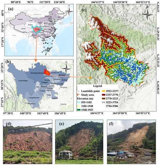
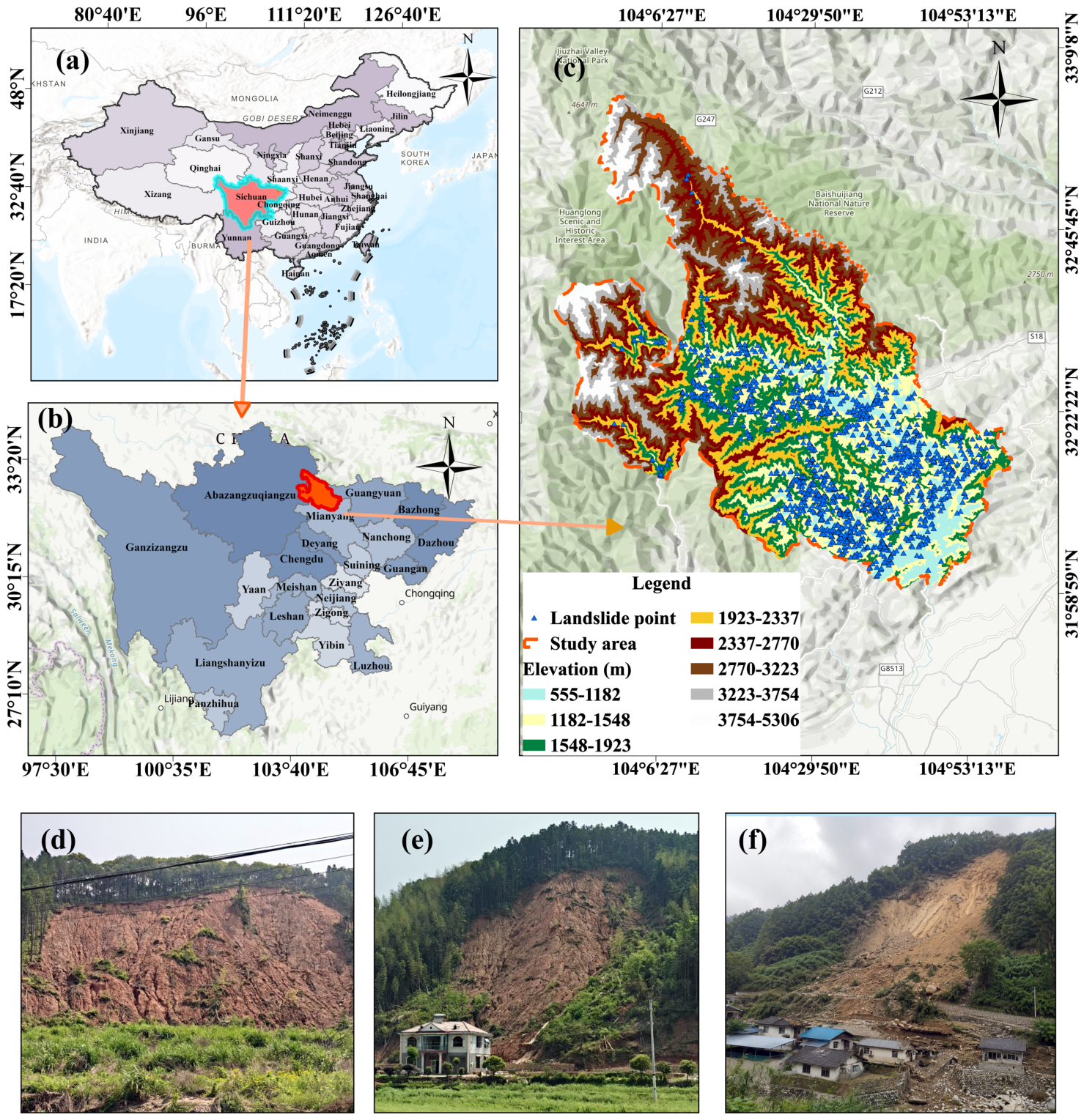
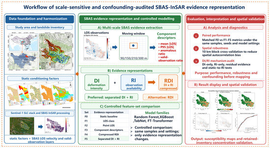
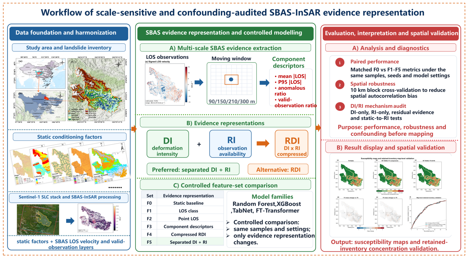
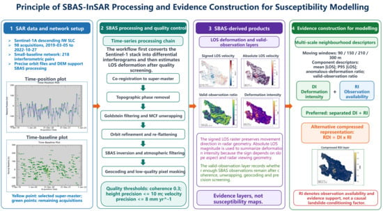
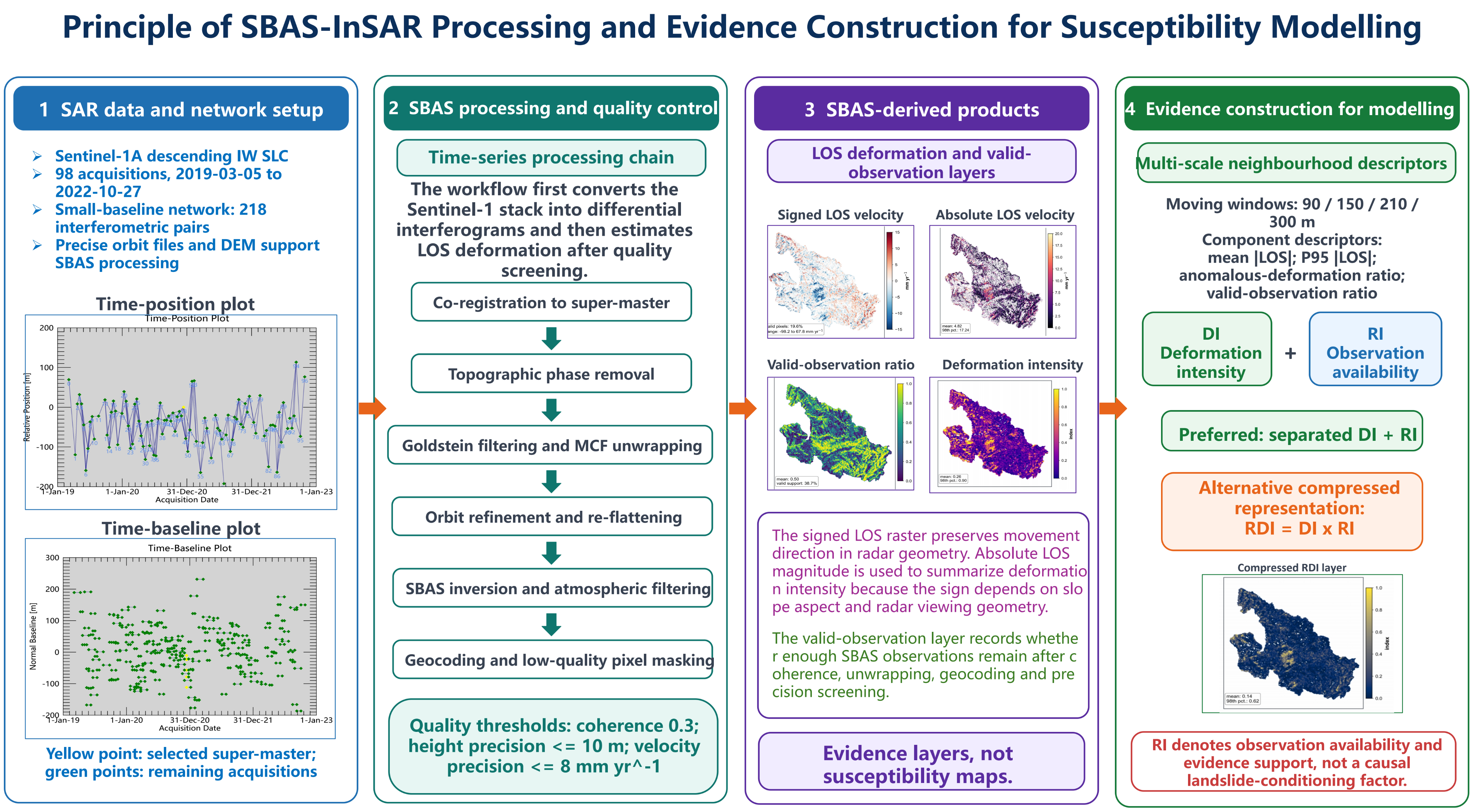
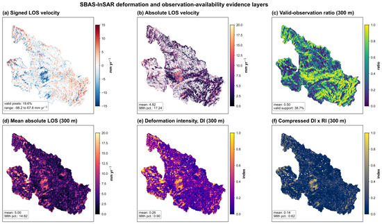
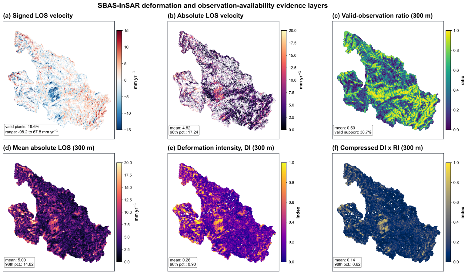
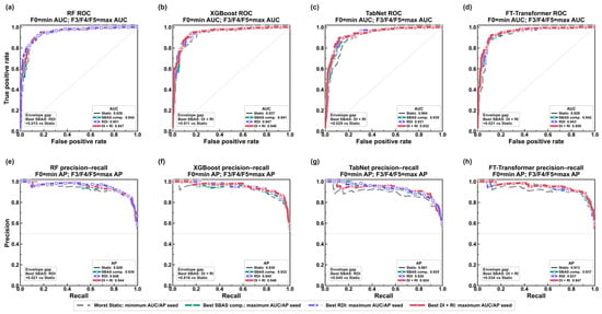
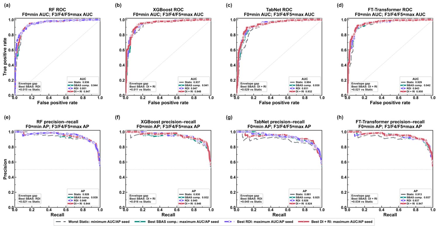
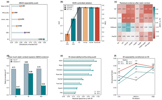
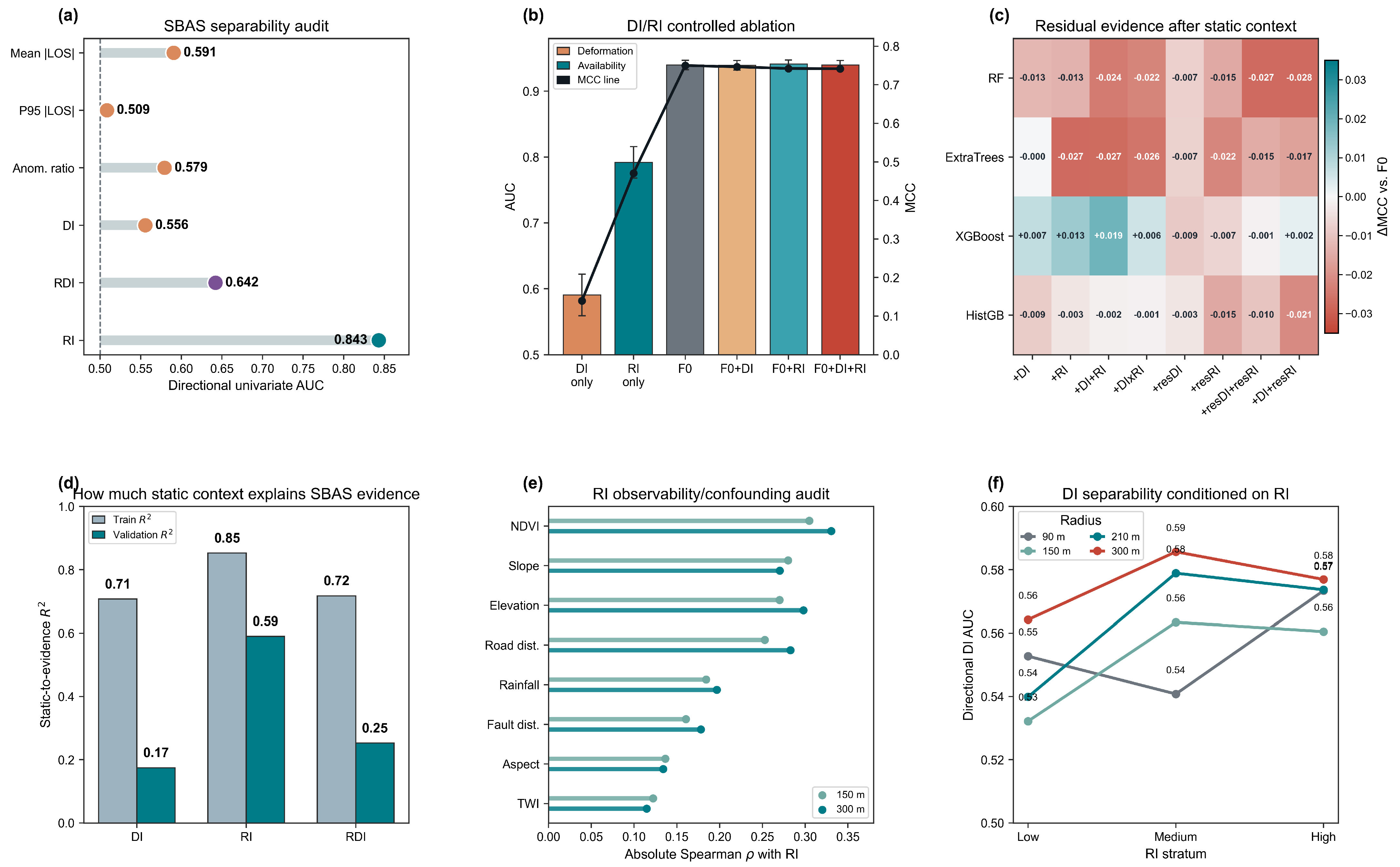
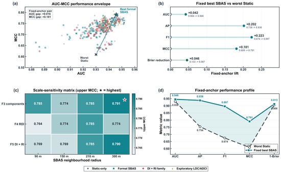
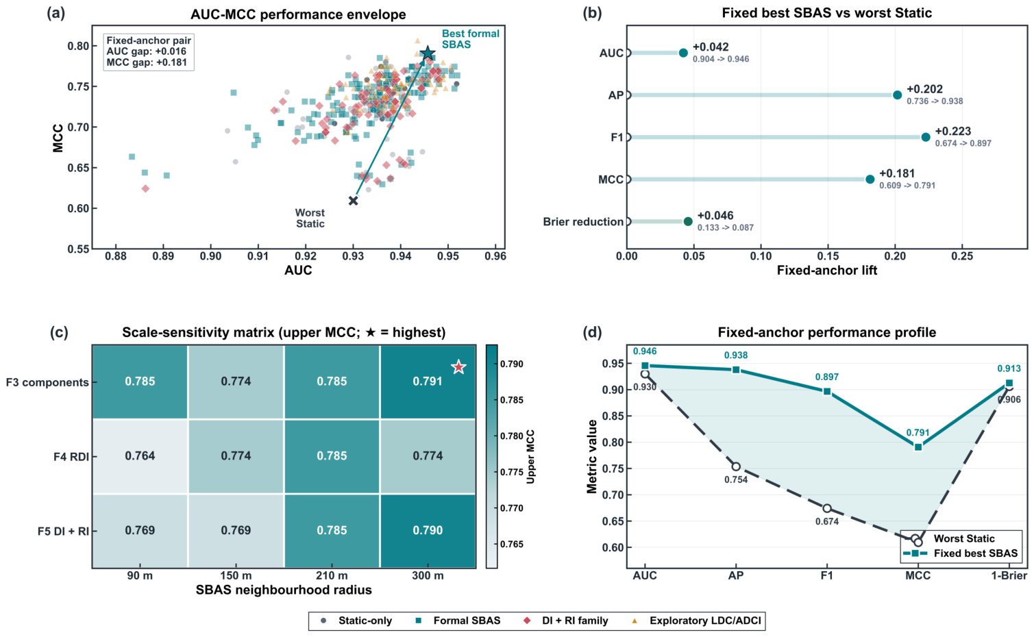
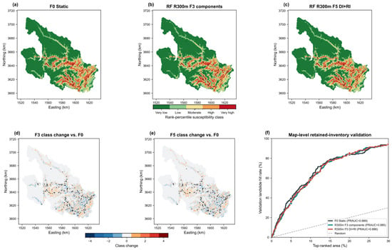
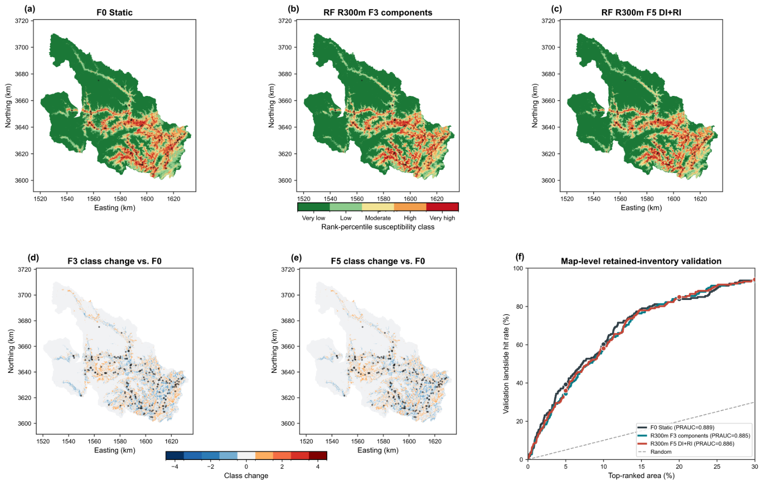

Disclaimer/Publisher’s Note: The statements, opinions and data contained in all publications are solely those of the individual author(s) and contributor(s) and not of MDPI and/or the editor(s). MDPI and/or the editor(s) disclaim responsibility for any injury to people or property resulting from any ideas, methods, instructions or products referred to in the content. |
© 2026 by the authors. Licensee MDPI, Basel, Switzerland. This article is an open access article distributed under the terms and conditions of the Creative Commons Attribution (CC BY) license.