Station-Level Gap Filling of TROPOMI NO₂ via Physics-Informed Shadow Manifold Reconstruction

Highlights

What are the main findings?

• A physics-grounded gap-filling framework reconstructs cloud-obscured TROPOMI NO₂ through manifold analogue inference on the atmospheric shadow attractor, achieving a 4.0–4.4× RMSE improvement over Random Forest baselines across ten European urban-background stations and returning Manifold Overlap Ratio (MOR_ext) values of 0.70–0.91, compared with consistently near-zero (median < 0.05) for all evaluated non-EDM methods—a separation exceeding 5×—across >3600 evaluations under the tested parameterisation.
• Three-level temporal validation—within-window masking, cross-year transfer, and a strictly prospective COVID-19 holdout—demonstrates that the reconstructed attractor remains physical under out-of-distribution perturbations: COVID-19 trajectories occupy the summer corner of the pre-COVID-19 library attractor, and DJF 2023/24 biases stratify into three mechanistically distinct classes reflecting library representativeness rather than model fragility.

What are the implications of the main findings?

• The MOR_ext categorical discriminator exposes a fundamental divide between dynamically coherent and merely accurate gap fillers, with direct consequences for downstream applications: exceedance detection, source attribution, exposure assessment, and process studies require preserved attractor geometry, not just low pointwise error.
• Built-in failure diagnostics (out-of-manifold flags, spatial-mismatch negative controls, explicit library-coverage checks) turn transfer biases into physically interpretable quantities, supporting transparent operational deployment of satellite NO₂ products and opening a reusable template for nonlinear-dynamics-based gap filling of other trace-gas retrievals.

Abstract

Cloud and quality screening removes approximately 65% of daily TROPOMI tropospheric NO₂ pixels, creating structured data gaps that coincide with meteorological conditions driving pollution extremes. Standard gap-filling methods—kriging, Random Forests and other machine learning methods—act as statistical smoothers that systematically suppress extreme concentrations and ignore the Missing Not At Random (MNAR) character of cloud-induced missingness. Here we present a physically informed framework that treats urban NO₂ as a forced nonlinear dynamical system and reconstructs missing satellite observations through geometric navigation on a shadow manifold rather than statistical interpolation. The framework integrates five components: (i) Multivariate State-Space Reconstruction (MSSR) using multiview embeddings of continuous ground-based NO₂, O₃, and ERA5 meteorology, grounded in Stark’s forced-system embedding theorem; (ii) Short-Time Regime-Conditioned Convergent Cross Mapping (ST-RC-CCM) with a spatial-mismatch negative control for falsifiable causal validation; (iii) Inverse Probability Weighting (IPW) to correct the clear-sky sampling bias; (iv) trajectory-matrix denoising via Singular Spectrum Analysis (SSA) and Robust PCA; (v) topology-inspired fidelity metrics—Manifold Overlap Ratio (MOR) and Dynamic Trend Capture (DTC)—that penalize smoothing artefacts. The physical basis for this coupling is the shared dynamical history of surface and column NO₂: tropospheric NO₂ has a photochemical lifetime of 1–4 h near urban emission sources, comparable to the boundary layer mixing timescale, ensuring that surface and column concentrations are jointly governed by the same emission–photolysis–transport attractor. The planetary boundary layer height (PBLH), solar zenith angle (SZA), and surface O₃—all included as MSSR coordinates—are the dominant physical drivers of the instantaneous surface-to-column scaling, and their joint trajectory in state space constitutes the physically grounded basis for analogue selection. The framework is validated on a synthetic forced Lorenz-96 system, then applied to five European primary cities spanning contrasting regimes (Sofia, Milano, Stuttgart, Kraków, Hamburg) plus five N1 spatial-mismatch control stations (Plovdiv, Genova, Frankfurt, Warszawa, Berlin)—ten urban-background stations across four countries—with structured ablations (A0-A4V-A4K). Across >3600 evaluations, MOR_ext distributions for EDM and non-EDM methods are non-overlapping by a factor exceeding 5× (EDM minimum 0.59 vs. non-EDM maximum 0.10; median non-EDM MOR_ext ≤ 0.05 at every city × mask combination), while EDM achieves MOR_ext up to 0.915 (Milano Po Valley). Under a fair-comparison benchmark that withholds ground-level NO₂ from Random Forest, EDM’s RMSE advantage remains robust at a median of 3.9× (RF_FULL) and increases to 4.2× (RF_METEO), confirming that the performance gap is physical rather than an information artefact. A three-level temporal validation—within-window pseudo-cloud masking, cross-year transfer (full 2022 holdout and DJF 2023/24), and a COVID-19 out-of-distribution test—demonstrates robustness beyond standard train/test splits, with CCM library-length convergence confirmed for 60/60 ablations (p < 0.001) across all ten stations. Spatial-mismatch tests confirm local dynamical specificity at all five primary–control pairs (Δρ = 0.090–0.210), with seasonal modulation driven by orographic and synoptic mechanisms. These results establish manifold-based gap filling as a dynamically informative complement to statistical approaches, particularly in topographically confined, stagnation-prone basins where preserving extreme-event geometry is essential for exposure assessment.

1. Introduction

1.1. The Operational Challenge: Beyond Smooth Interpolation

Nitrogen dioxide (NO₂) is a key trace gas in Earth’s troposphere that plays a central role in air quality in urban areas and in the formation of secondary aerosols, and serves as a critical indicator of human activity. The Sentinel-5 Precursor satellite, carrying the TROPOMI instrument, has revolutionized our ability to observe NO₂ columns in the troposphere with an unprecedented spatial resolution of 5.5 × 3.5 km² at nadir [1,2]. The operational retrieval first derives tropospheric NO₂ slant column densities (SCDs) using Differential Optical Absorption Spectroscopy (DOAS) in the 405–465 nm spectral window; these are subsequently converted to vertical column densities (VCDs) via stratospheric–tropospheric separation and air mass factor (AMF) correction [3,4]. However, the applicability of TROPOMI data is limited by the characteristics of passive optical remote sensing, particularly sensitivity to cloud cover, aerosols, and observation geometry. Valid measurements require clear or mostly clear skies, as clouds obscure the lower troposphere, where most anthropogenic NO₂ is concentrated. The standard quality assurance (QA) filter (qa_value > 0.75) removes approximately 65% of daily pixels globally [5]. In temperate latitudes, cloud cover, aerosol loading, and extraction artefacts can render 50–70% of winter observations unusable [6]. These gaps are not randomly distributed but are structurally correlated with meteorological systems—frontal passages, convective storms, and persistent stratiform cloud cover—which themselves are driving factors for pollutant dispersion and chemical transformation [7]. The resulting lack of connectivity makes it difficult to calculate reliable exposure estimates, validate chemical transport models, and monitor transient emission events.

Current operational approaches for filling gaps in satellite data and standard machine learning (ML) algorithms often fail to preserve the discontinuous and highly variable nature of NO₂ spatiotemporal distributions, including local extreme concentrations. Traditional geostatistical spatiotemporal interpolations (e.g., Kriging) and global machine learning models implicitly favour statistical smoothing. By treating missing data as a stochastic error that must be smoothed out, these methods act as low-pass filters that systematically suppress extreme events. Crucially, they do not account for the fact that missing satellite data are “Missing Not At Random” (MNAR): cloud cover is physically linked to specific meteorological systems, such as the passage of fronts or thermal inversions, which directly determine the accumulation and dispersion of pollutants.

In this context, there is a need for methodological approaches that explicitly account for the nonlinear dynamics of atmospheric processes and the non-random nature of missing data, while preserving the physically significant extremes in the observed pollution fields.

1.2. Limitations of Current Gap-Filling Approaches

Current methodologies for filling satellite NO₂ data gaps fall into three categories, each with fundamental limitations regarding the preservation of atmospheric dynamics.

Geostatistical interpolation methods such as kriging and inverse distance weighting assume spatial or temporal autocorrelation and apply low-pass filters to the data field [8]. They smooth out the sharp gradients and high-frequency fluctuations that characterize turbulent diffusion of short-lived pollutants, leading to systematic underestimation of peak exposures. Chemical transport model (CTM) assimilation approaches encapsulate fundamental physical equations but are limited by emission inventory resolution (typically 10–50 km), subject to boundary condition biases, and computationally expensive—and carry structural model errors in turbulence parameterisation, chemical mechanisms, and dry deposition schemes that persist even under idealized boundary conditions and emissions inventories [9,10]. Machine learning approaches—most prominently Random Forests trained with MSE objectives, the most widely used configuration in the TROPOMI gap-filling literature—excel at pattern recognition but function as sophisticated smoothers that systematically suppress variance by construction, a structural consequence of pointwise loss minimisation that is independent of their pointwise accuracy and holds regardless of feature engineering [11,12,13,14].

A shared limitation across all three paradigms is the implicit assumption that satellite data gaps are Missing at Random (MAR). This assumption is contradicted by documented evidence. Geddes et al. [7] showed that cloud-based filtering of OMI causes systematic NO₂ underestimation of 12% in urban areas, 20% in suburban areas, and up to 40% in rural settings. Goldberg et al. [15] found that surface NO₂ concentrations are 17% higher on average across all days compared to clear-sky days, and 36% higher on cloudy days specifically. This clear-sky bias represents a Missing Not At Random (MNAR) mechanism: the probability of a valid satellite observation depends on the atmospheric state itself. To our knowledge, no existing gap-filling method for satellite NO₂ data explicitly addresses this bias. Nonlinear dynamical methods also appear not to be applied, and the attractor structure of the underlying pollution–meteorology system has not yet been exploited.

1.3. A Different Approach: Gap Filling as Geometric Navigation

This study proposes an alternative framework grounded in Empirical Dynamic Modelling (EDM) [16,17,18,19], a set of methods from nonlinear dynamical systems theory. The central idea is conceptually straightforward, though its mathematical foundations are rigorous [16,18,19].

In a coupled atmospheric system, the time history of a continuously observed variable—such as hourly ground-level NO₂—encodes information about all interacting drivers through the geometry of its trajectory in a reconstructed state space. This principle, established by Takens’ Embedding Theorem [20], means that by constructing time-delayed coordinate vectors from continuous ground measurements, we can build a “shadow manifold” that is topologically equivalent to the true atmospheric attractor. Surface measurements and satellite column observations, being different projections of the same atmospheric state, share this dynamical structure.

The practical implication for gap filling is direct. When clouds obscure the satellite at a given time, the continuous ground station continues to trace the system’s trajectory on the shadow manifold. By locating the current atmospheric state on this manifold and identifying historical analogues—past moments when the atmosphere exhibited the same dynamical signature and the satellite view was clear—we can project those historical satellite values to fill the current gap. This transforms gap filling from a statistical interpolation problem into a geometric navigation task on the reconstructed attractor, naturally preserving extreme events and high-frequency variability that statistical methods smooth away. Crucially, this is not a surface-to-column regression: MSSR does not estimate a transfer function between surface and column NO₂. Instead, it navigates a reconstructed phase space in which surface observations and satellite columns are projections of the same dynamical attractor, and gap filling consists of retrieving historical TROPOMI values at dynamically equivalent past states—not applying a learned mapping across sky conditions.

Two critical physical challenges must be addressed for this approach to work in practice. First, atmospheric NO₂ is a non-autonomous system whose dynamics change with solar geometry (controlling photolysis rates) and boundary layer conditions (controlling mixing volume and surface-to-column relationships). Applying standard embedding methods without accounting for this forcing would mix dynamically distinct regimes—creating what we term “dynamical chimeras” where winter stagnation analogues are erroneously matched to summer photochemistry episodes. We address this using the forced-system embedding framework of Stark [21,22], which provides theoretical justification for including forcing variables (solar zenith angle, planetary boundary layer height) as explicit coordinates or neighbourhood constraints in the reconstructed state space.

Second, the manifold-based reconstruction is only physically justified when a genuine dynamical coupling exists between the ground and satellite observation systems. We verify this using Convergent Cross Mapping (CCM) [23], which tests whether the shadow manifold of one variable contains sufficient information to reconstruct the states of another. In our framework, CCM serves as an operational quality-control filter: imputation is performed only in time windows where CCM diagnostics confirm that the ground–satellite coupling is stable [24].

1.4. What This Paper Delivers

This paper contributes the following:

• An explainable, station-level method for reconstructing cloud-gapped TROPOMI tropospheric NO₂ using regime-aware state-space reconstruction from continuous ground NO₂/O₃ and a minimal meteorological forcing set (winds, SZA, PBLH from ERA5).
• A built-in validity diagnostic based on short-time, regime-conditioned CCM with a spatial-mismatch negative control that tests whether detected coupling reflects genuine local physics or shared large-scale forcing.
• Explicit MNAR bias correction via stabilized IPW integrated into the analogue weighting scheme, addressing the documented clear-sky sampling bias.
• Phase-space denoising (SSA/Robust PCA) that separates instrument noise from deterministic dynamics without smoothing pollution plumes.
• Calibrated anti-smoothing evaluation metrics (MOR, DTC) that explicitly penalize gap-filling methods achieving low error by flattening peaks, validated on a synthetic forced Lorenz-96 system.
• A head-to-head comparison with a Random Forest baseline demonstrating that EDM produces a median RMSE advantage of 4.0× over RF, increasing to 4.4× in a fair-comparison benchmark that withholds ground-level NO₂ from the RF features—establishing the advantage as physical rather than informational.
• A three-level temporal validation strategy comprising within-window pseudo-cloud masking, cross-year transfer tests (full held-out year and held-out winter), and a COVID-19 out-of-distribution test using only pre-event data—demonstrating robustness beyond standard train/test splits.
• A reproducible experimental design with structured ablations (A0-A4V-A4K) across five European primary cities (Sofia, Milano, Stuttgart, Kraków, Hamburg) supplemented by five N1 spatial-mismatch control stations (Plovdiv, Genova, Frankfurt, Warszawa, Berlin), yielding ten urban-background stations that span basin stagnation, Po Valley mixed photochemistry, continental basin, coal-heating, and maritime advection regimes.

The remainder of this paper is organized as follows. Section 2 provides the theoretical background. Section 3 presents Materials and Methods, comprising study area, data, methods, and experimental design. Section 4 presents results. Section 5 discusses physical interpretation, comparison with machine learning, regime-dependent performance, transfer-bias mechanisms, and limitations. Section 6 concludes the paper.

2. Background and Theoretical Basis

This section provides the conceptual foundations underlying the methodology. The emphasis is on physical intuition and practical relevance rather than formal proofs, which are available in the cited primary literature. Readers primarily interested in implementation may proceed directly to Section 3.3.

2.1. Delay Embedding: Reconstructing System Dynamics from a Single Sensor

The atmosphere behaves as a dissipative dynamical system whose state evolves on a lower-dimensional attractor within a high-dimensional phase space [25]. For a dynamical system evolving on a d-dimensional manifold M, Takens [20] proved that the state space can be reconstructed from a single scalar time series x(t) using time-delayed coordinates. The reconstructed state vector Y(t) in an m-dimensional embedding space is defined as

Y(t) = [x(t), x(t − τ), x(t − 2τ), …, x(t − (m − 1)τ)]

where τ is the time lag and m is the embedding dimension. If m ≥ 2d + 1, the reconstructed shadow manifold MY is generically diffeomorphic to the true manifold M [20]. Sauer et al. [26] extended this to fractal attractors, proving that m > 2d suffices in the stronger sense of prevalence. For atmospheric attractors, which may have fractal dimension, this relaxation has practical importance.

The practical significance for remote sensing is direct: neighbouring points on the shadow manifold correspond to genuinely similar atmospheric states—not merely moments with similar concentrations, but states where the atmosphere was evolving under the same dynamical rules. The delay τ is selected at the first minimum of the average mutual information function [27], and m is diagnosed via False Nearest Neighbours (FNNs) [28,29] or Cao’s threshold-free method [30]. Johnson and Munch [31] demonstrated that EDM can be adapted to handle missing or irregularly sampled data, providing a direct precedent for the gap-filling application developed here.

2.2. Stark’s Embedding Theorem for Forced Systems

Atmospheric NO₂ is non-autonomous: its dynamics are driven by time-varying SZA, PBLH, and weather. Classical Takens embedding can produce trajectory crossings where dynamically distinct states appear as False Nearest Neighbours [29].

Stark [21] resolved this by treating the forced system as an autonomous skew-product flow on the product space P × M:

$$\mathit{F}\left(\mathit{p},\mathit{x}\right)=\left(\mathit{\sigma }\left(\mathit{p}\right),\left({\mathit{f}}_{\mathit{p}}\right(\mathit{x})\right)$$

where P is the forcing space and M is the response space. When forcing is directly observed—as when ERA5 reanalysis is available—only ~2 dim M + 1 delays are needed [21,22].

Stark proved two critical results [21,22]. First, when forcing is unknown, approximately 2(dim P + dim M) + 1 delay coordinates of the response variable suffice to reconstruct the full product-space attractor. Second, when forcing is known (the “bundle embedding”), only ~2 dim M + 1 delays of the response are needed because forcing dimensions are captured by direct observation—precisely the situation when meteorological data are available from reanalysis products.

Stark’s stochastic extension [22] covers the case where forcing contains random components, relevant because atmospheric forcing includes both deterministic (solar cycle) and stochastic (turbulent transport) elements. When the response contracts under forcing—as occurs when NO₂ “synchronizes” to meteorological conditions—the attractor takes the form of an invariant graph γ: P → M, meaning the response state is determined by the forcing state [31].

In practical terms, this justifies including SZA (photolysis control) and PBLH (mixing volume) as explicit coordinates or kernel variables. SZA ensures analogues come from the same photochemical regime; PBLH prevents conflating well-mixed and stratified states. The multivariate embedding generalization of Deyle and Sugihara [32] further establishes that delay vectors from multiple coupled time series yield valid reconstructions with fewer lags per variable.

2.3. Convergent Cross Mapping as a Validity Diagnostic

Before using the ground-based manifold to reconstruct satellite observations, we must verify genuine dynamical coupling. CCM [23] tests whether the shadow manifold of one variable can reconstruct the states of another. The critical diagnostic is convergence: skill ρ must increase with library size L. The direction is informative: if X drives Y, then MY cross-maps to X [33].

CCM is sensitive to shared seasonal periodicity [34,35]. We mitigate this through: (i) time-lagged CCM for directionality [23], (ii) seasonal surrogate testing [36], (iii) short-time windows restricting analysis to comparable forcing states, and (iv) a spatial-mismatch negative control (Section 3.3.7).

In our operational pipeline, CCM acts as a rigorous, physics-based quality-control (QC) filter. It ensures the method does not hallucinate data. If a ground station becomes decoupled from the satellite pixel (e.g., due to extreme horizontal advection blowing a plume over the pixel without touching the surface sensor), the CCM convergence test fails. The algorithm immediately flags this state as “out-of-manifold” and safely refuses to perform the reconstruction, offering a transparent alternative to the overconfident extrapolations typical of purely statistical methods.

2.4. Singular Spectrum Analysis for Trajectory-Matrix Denoising

Remote sensing algorithms must acknowledge hardware realities. TROPOMI retrievals contain heteroskedastic measurement noise (varying with cloud fraction, SZA, and surface albedo), while ground sensors exhibit slow calibration drift. If noise is not separated from the deterministic signal before manifold reconstruction, the shadow manifold becomes “thickened”: nearest neighbours reflect noise proximity rather than dynamical similarity, corrupting both CCM causal inference and gap-filling predictions [37,38].

To address this, we introduce a noise-reduction step performed directly in the phase space prior to embedding. Broomhead and King [37] introduced Singular Spectrum Analysis (SSA) in the context of nonlinear dynamics, explicitly grounding the method in Takens’ theorem. We construct a trajectory matrix (Hankel matrix) from the time series and apply SSA and Robust Principal Component Analysis (RPCA) [39]. By utilizing the singular value “noise floor,” we project the data onto a low-rank subspace that represents the true deterministic skeleton of the atmospheric attractor.

Because low-rank SSA can treat sharp NO₂ plumes as “noise,” we additionally implement Robust PCA, which decomposes H = L + S into a low-rank component L (deterministic manifold skeleton) and a sparse component S (spikes/extremes). We use L for CCM and neighbour selection while retaining S for stress-testing extreme-event fidelity, ensuring that denoising does not “win by smoothing.”

2.5. The MNAR Problem in Satellite Observations

A major vulnerability in satellite data retrieval is the sampling bias introduced by clouds. Because TROPOMI requires clear skies for valid measurements, the historical “anchor library” available for analogue matching is overwhelmingly skewed toward clear-weather dynamics. However, cloud cover is physically tied to specific meteorological systems (such as thermal inversions and frontal passages) that directly govern pollutant accumulation. Thus, satellite data missingness is Missing Not At Random (MNAR). Training a model exclusively on clear-sky data leads to cloud-driven bias, systematically underestimating the severe smog episodes that occur during cloudy winter days.

To mathematically correct this bias, we implement Inverse Probability Weighting (IPW) [40,41] directly into the manifold operators. The framework first estimates the observation probability $\widehat{\mathit{\pi }}$—the likelihood that the satellite will successfully record a valid pixel under specific weather and photolytic conditions. The IPW kernel is then computed as the inverse of this probability (1⁄$\widehat{\mathit{\pi }}$). In practice, this means the algorithm assigns a substantially higher mathematical weight to the rare historical analogues that represent heavily clouded, stagnant, or difficult atmospheric states. By artificially boosting the importance of the few historical cloudy days available on record, the IPW kernel forces the model to rely on accurate, weather-appropriate analogues when reconstructing a new cloudy-day gap.

3. Materials and Methods

3.1. Study Sites

This study operates at the station level, reconstructing temporal NO₂ dynamics at individual monitoring sites without spatial coupling between stations or pixels. This deliberate scope focuses on establishing the foundations of dynamical gap filling at the point scale before future extension to spatially resolved products via multispatial CCM [42] or geographical CCM [24].

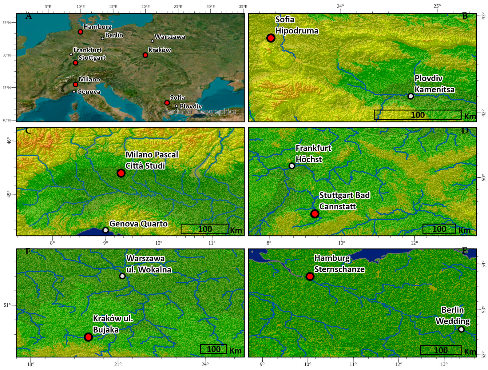
Five European primary cities across four countries were selected to represent distinct atmospheric regimes, each instrumented with one EEA urban-background (UB) station. These are supplemented by five N1 spatial-mismatch control stations located 100–250 km from each primary site across distinct orographic or synoptic boundaries, yielding ten stations in total. Urban-background stations reduce micro-scale roadside variability and improve representativeness at the TROPOMI pixel scale. The single-station-per-city design maximizes regime diversity—five independent atmospheric regimes plus five control pairs—providing stronger evidence for method generalizability (Figure 1).

 Primary Cities (5 Urban Background Stations) 

Sofia, Bulgaria (BG0050A Hipodruma, 42.68°N, 23.30°E, ~550 m a.s.l.): It is located in an intermontane basin, surrounded by mountain ranges that strongly limit ventilation. Winter conditions are frequently characterized by temperature inversions, weak winds, and planetary boundary layer heights below 300 m, which trap pollutants and create persistent cloudiness. Sofia represents a stagnation-dominated regime with mean annual NO₂ of 35–45 µg/m³.

Milano, Italy (IT1692A Pascal Città Studi, 45.48°N, 9.24°E, ~120 m a.s.l.): It is located in the central Po Valley, bounded by the Alps and Apennines. Winter fog and inversions combine with summer photochemical smog to produce among the highest NO₂ concentrations in Europe (40–55 µg/m³). Milano represents a mixed photochemistry–stagnation regime.

Stuttgart, Germany (DEBW013 Bad Cannstatt, 48.81°N, 9.23°E, ~220 m a.s.l.): It is located in the Stuttgarter Kessel, a topographic basin within the Neckar valley. The surrounding hills create a natural bowl that traps pollutants during frequent temperature inversions, analogous to Sofia but in a Western European continental setting. Stuttgart represents a continental basin regime with mean annual NO₂ of 28–38 µg/m³.

Kraków, Poland (PL0501A ul. Bujaka, 50.01°N, 19.95°E, ~200 m a.s.l.): It is located in the Vistula valley at the northern edge of the Carpathian foothills. Frequent winter inversions combine with significant residential coal-heating emissions—a distinctly Eastern European source profile that produces a characteristic evening emission peak absent from traffic-dominated cities. Kraków represents a cold continental with coal-heating regime with mean annual NO₂ of 30–45 µg/m³.

Hamburg, Germany (DEHH008 Sternschanze, 53.56°N, 9.97°E, ~15 m a.s.l.): It is located on the Elbe estuary, approximately 100 km from the North Sea. Flat terrain and persistent westerly winds create strong horizontal ventilation with mean wind speeds 2–3× higher than the basin cities. Frontal systems pass every 3–5 days, producing short but frequent cloud gaps in TROPOMI. Hamburg represents a maritime advection regime with mean annual NO₂ of 25–33 µg/m³.

 N1 Spatial-Mismatch Control Stations (5 Urban Background Stations) 

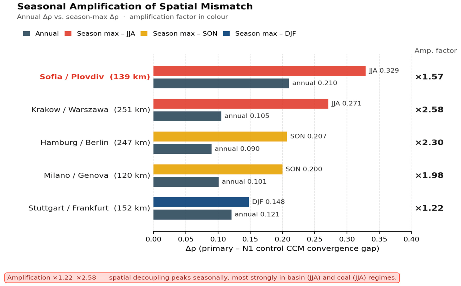
Each primary city is paired with a control station located 100–250 km away across a distinct orographic or synoptic boundary. The control-station design enables a falsifiable spatial-specificity test (Section 4.4): the reconstructed manifold of a primary city should degrade when mapped to a TROPOMI pixel drawn from a dynamically distinct regime, confirming that the EDM framework encodes local rather than regional dynamics.

Plovdiv, Bulgaria (BG0051A, 42.15°N, 24.75°E): Upper Thracian Plain, ~130 km southeast of Sofia across the Sredna Gora mountain ridge; mean elevation ~160 m a.s.l.; open plain topography—opposite regime to Sofia’s basin stagnation—provides a stringent orographic decoupling control.

Genova, Italy (IT0858A, 44.41°N, 8.93°E): Ligurian coastal urban centre, ~120 km south of Milano across the Apennine ridge; mean elevation ~20 m a.s.l.; maritime–orographic contrast with Po Valley continental conditions.

Frankfurt am Main, Germany (DEHE005, 50.11°N, 8.68°E): Rhine-Main Basin, ~150 km north of Stuttgart across the Schwarzwald; mean elevation ~95 m a.s.l.; larger open basin and transcontinental transport corridor contrast with Stuttgart’s enclosed Neckar bowl.

Warszawa, Poland (PL0141A, 52.23°N, 21.01°E): Mazovian Lowland, ~250 km north of Kraków; mean elevation ~100 m a.s.l.; continental plain contrasts with the Vistula valley coal-heating regime.

Berlin, Germany (DEBE010, 52.52°N, 13.40°E): Continental urban centre, ~250 km southeast of Hamburg; mean elevation ~35 m a.s.l.; continental lowland contrasts with Hamburg’s maritime advection regime.

This ten-station design spans the full European ventilation spectrum from basin stagnation (Sofia, Stuttgart) through mixed regimes (Milano, Kraków) to maritime advection (Hamburg), with each primary city paired to a geographically proximate but dynamically distinct control station for rigorous spatial-specificity testing.

3.2. Data

3.2.1. TROPOMI Tropospheric NO₂

We use TROPOMI Level-2 tropospheric NO₂ VCD retrievals (product version v2.4+) at overpass times (~13:30 local time) for 2019–2024 [1,3,4]. Only pixels with qa_value > 0.75 are retained [5]. The retrieval uncertainty proxy σ_(S(t)) is retained for heteroskedastic weighting. For each station and overpass, candidate pixels within 10 km are identified; the pixel with maximum QA (tie-broken by minimum distance) is selected. If no pixel passes QA, the observation is missing. Colocation distances between selected pixel centroids and station coordinates range from 2.31 to 2.61 km (median of station medians = 2.47 km) across all ten stations (Supplementary Table S3). At the operational 10 km search radius, the number of valid overpasses meeting QA criteria (qa_value > 0.75) ranges from 779 (Warszawa) to 1513 (Plovdiv) per station over the 2019–2024 study period. Tightening the search radius to 5 km retains 79–90% of overpasses; a 2 km radius retains only 33–40%, reducing the MSSR library below the minimum required for stable CCM convergence (N_lib ≥ 80) at most stations. The 10 km radius therefore represents the operational minimum for this dataset and station network.

3.2.2. EEA Ground-Level NO₂ and O₃

Hourly NO₂ and O₃ data are retrieved from the EEA air quality e-Reporting level E1a database, restricted to urban-background stations. O₃ is included because the NO₂-O₃ photostationary state encodes photolytic regime information: the NO₂/O₃ ratio resolves ambiguity when low NO₂ may indicate either clean air or rapid photolytic depletion. Standard QC: flagged/negative values are removed; gaps < 3 h are filled by linear interpolation; longer gaps are excluded.

A notable data-availability constraint concerns station PL0141A (Warszawa) during 2022. An independent quality control confirmed that all 4639 hourly records for that calendar year carry the EEA Validity flag −1 with placeholder value −999 µg m⁻³, and the period June–September 2022 is absent entirely from the e-Reporting record. Two independent downloads from the EEA database confirmed this outage. This station–year combination is therefore excluded from the year-holdout transfer test (XYA) for Warszawa but retained for the MCAR ablation, DJF 2023/24 transfer (XYB), and COVID-19 transfer (XYC) because those windows are unaffected. Section 3.3.11 describes how this constraint is converted into a methodological strength: the framework reports no prediction where no verified reference exists, consistent with the EDM design philosophy of transparent uncertainty quantification.

3.2.3. ERA5 Meteorological Forcing

Three meteorological variables capture the essential physical controls on NO₂ variability (

Table 1. Meteorological variables used in the framework.

Variable	Source	Code	Physical Role
10 m zonal wind	ERA5-Land	u10	Horizontal transport and advection
10 m meridional wind	ERA5-Land	v10	Horizontal transport and advection
Boundary layer height	ERA5 single levels	blh	Vertical-mixing volume; surface-to-column scaling

): 10 m zonal wind (u10) and meridional wind (v10) from ERA5-Land [43] at the nearest gridpoint encode horizontal transport and advection; boundary layer height (blh) from ERA5 single levels [44] captures vertical-mixing volume and surface-to-column scaling. Solar zenith angle (SZA) is computed deterministically from station coordinates and UTC time. Seasonal phase is encoded as

$$\mathit{p}\left(\mathit{t}\right)=\left[\mathbf{cos}\left({\displaystyle \frac{\mathbf{2}\mathit{\pi }·\mathit{D}\mathit{O}\mathit{Y}}{\mathbf{365}}}\right),\mathbf{sin}\left({\displaystyle \frac{\mathbf{2}\mathit{\pi }·\mathit{D}\mathit{O}\mathit{Y}}{\mathbf{365}}}\right)\right]$$

This minimal set captures horizontal transport (winds) and vertical mixing (PBLH). Additional ERA5 variables (temperature, humidity, pressure, cloud cover, precipitation, radiation) are deliberately excluded: their influence is largely captured indirectly through PBLH (integrating thermodynamic stability) and SZA (encoding actinic flux). Including them would risk the curse of dimensionality in the multiview reconstruction. Cloud information is implicitly reflected in the QA-based missingness indicator M(t). This choice is evaluated via ablation (Section 3.3.10).

3.2.4. Time Alignment

All data streams are aligned to the TROPOMI overpass time: ground NO₂/O₃: nearest hour (|t − t̃| ≤ 30 min); ERA5: nearest hourly field; SZA: exact overpass time. For the hourly MSSR embedding, the full continuous ground and ERA5 series are used without overpass restriction, as the shadow manifold requires continuous temporal coverage.

3.3. Methods

The pipeline described in the following subsections performs analogue inference on a reconstructed attractor—not statistical regression from surface to column. At each gap-filled time step, the algorithm identifies past overpasses at which the atmosphere was in a dynamically equivalent state and the satellite view was unobstructed, then transfers those historical TROPOMI VCD values directly. No surface-to-column mapping is fitted, trained, or applied across sky conditions.

3.3.1. Processing Pipeline Overview

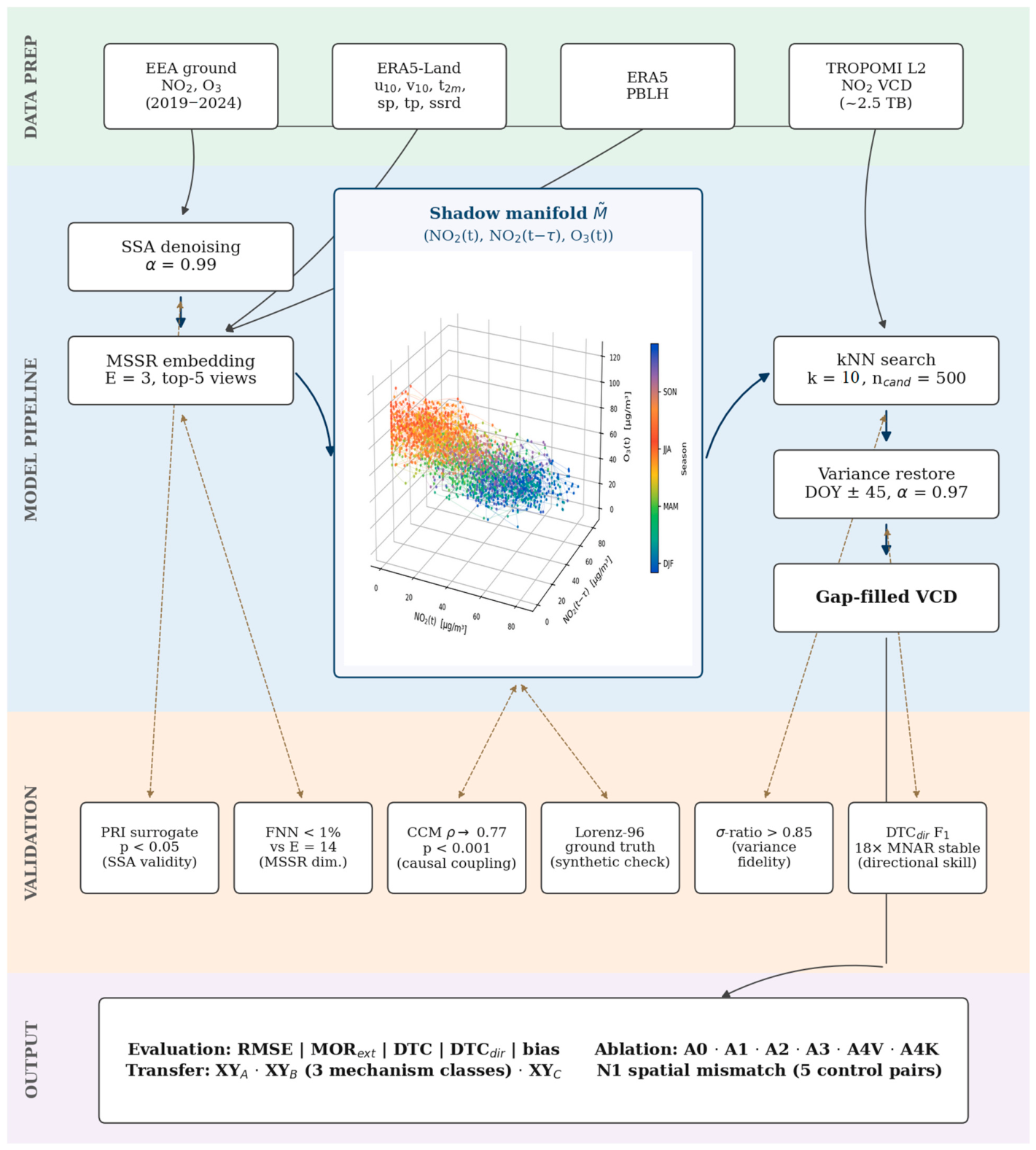
The station-level pipeline consists of eight sequential steps: (1) phase-space denoising via SSA/RPCA trajectory-matrix decomposition; (2) state-space reconstruction via MSSR multiview embedding with FNN diagnostics; (3) regime characterization using the Photolytic Regime Index; (4) missingness modelling via stabilized IPW; (5) causal validation via ST-RC-CCM with spatial-mismatch control; (6) gap filling through manifold-based analogue imputation with forcing-consistent weighting; (7) quality assessment using MOR, DTC, and conventional metrics; (8) structured ablation and sensitivity analysis. All pipeline hyperparameters with values, code-verified sources, and sensitivity references are consolidated in Supplementary Table S4.

Figure 2 depicts the end-to-end processing pipeline from raw TROPOMI retrievals and ground-station records to gap-filled VCD with per-step quality-control flags. Steps 1–7 constitute the full theoretical framework; in the present ten-station implementation, SSA (Step 1) is the activated denoising method, RPCA spike-separation serves as an optional extension for future impulsive-source environments, and the stabilized IPW propensity model (Step 4) is fully validated for the primary Sofia station while the remaining nine stations use the A4K boundary-layer-height kernel as the operationally deployed MNAR correction. These implementation choices do not affect the generality of the framework or the interpretation of the results.

The pipeline is implemented in Julia 1.10 for all EDM components (SSA, MSSR, CCM, gap filling, metrics) and Python 3.11 for data preprocessing, RF baseline, and figures. Julia was selected for three workload-specific reasons: (i) KDTree-based k-nearest-neighbour operations (NearestNeighbors.jl) achieve C-level performance for the low-dimensional embeddings (d = 3–7) and moderate library sizes (N ≈ 800–1300) characteristic of this dataset; (ii) the CCM surrogate loop (500 surrogates × 7 library fractions × 6 replicates per ablation) executes as a tight numerical loop without interpreter overhead; (iii) the Arrow IPC format provides zero-copy Python–Julia data exchange. Observed wall-clock times on a standard workstation (single CPU core): SSA denoising ~5 s per station; MSSR view selection (N_CAND = 500) ~15–20 min per station per ablation; CCM (60 ablations × 7 fractions × 6 replicates × 500 surrogates) ~2 h per station; gap filling (63 masks × 6 ablations) ~30 min per station; RF baseline (Python, scikit-learn, 500 trees) ~5–6 min per station. Full ten-station pipeline in serial execution: approximately 25–30 CPU-hours, reducible to approximately 4 h with station-level parallelisation across 10 cores.

3.3.2. Step 1: Phase-Space Denoising via Trajectory-Matrix SVD

For each scalar series y(t) in a processing window Ω of length N, we construct the Hankel matrix H(y) of size m × K with

$$H_{i,j}=y\left(t_j+(i-1)\delta \right).$$

The default is m = 48 (hourly, two diurnal cycles) or m = 30 (overpass resolution). Standard SSA performs

$$H=U\mathsf{\Sigma }{V}^T$$

and reconstructs

$$H_r=U_{1:r}{\mathsf{\Sigma }}_{1:r}{V}_{1:r}^T$$

with rank r at the spectral elbow (typically 4–8). Weighted SSA solves

$$min{\Vert W⨀(H-H_r)\Vert }_F^2$$

with weights

$$\omega (t)\propto {\displaystyle \frac{1}{{\sigma (t)}^2+{\epsilon }_{\sigma }}}$$

via IRLS. RPCA [40] solves

$$min{\Vert L\Vert }_{*}+\lambda {\Vert S\Vert }_1 \mathrm{s.t.} H=L+S$$

with

$$\lambda ={\displaystyle \frac{1}{\sqrt{\mathrm{m}\mathrm{a}\mathrm{x}(m,K)}}}.$$

L serves as the manifold; S preserves spikes. Denoising is accepted only when forecast skill improves without degrading MOR_ext or DTC.

In this study, the denoising step uses SSA exclusively (standard rank-r truncation with min_variance_kept = 0.99); the RPCA spike-separation component described in earlier framework versions is retained as a theoretically motivated extension for future work on impulsive-source environments but is not activated in the current results. The SSA is applied to the complete time series prior to library/test partitioning. At hourly temporal resolution (ground NO₂, ERA5 meteorology), rank r = 4–8 components account for ≥ 99% of variance, capturing the annual cycle and its harmonics. At overpass resolution (~1 observation per day, N ≈ 1300 per station), the sparser sampling distributes variance across more components: for the Sofia VCD series, rank r = 46 of 48 is required to retain ≥99% variance, meaning SSA functions as an approximate identity transform with minimal signal alteration. A dedicated numerical verification for Transfer Test A (2022 holdout) confirms that the RMSE between globally and library-restricted denoised series is 3.95 µmol m⁻², arising from a mathematical boundary reconstruction artefact (differing Hankel matrix dimensions K = 1278 vs. K = 1019) rather than from temporal information mixing. No temporal leakage is introduced by the global denoising step.

A dedicated numerical verification was conducted for Transfer Test A (2022 holdout, Sofia BG0050A). SSA was applied both globally (current implementation, N = 1325 overpasses) and with a library-restricted partition (N = 1067, excluding 2022 ± 30 days). The RMSE between the two denoised library-period series was 3.95 µmol m⁻², which, however, reflects a mathematical boundary reconstruction artefact rather than temporal leakage: at the overpass-level temporal resolution (one observation per day, m = 48 overpasses), the TROPOMI VCD series is structurally rich—requiring rank r = 46 of 48 SSA components to retain ≥ 99% variance. At this near-full rank, SSA functions as an approximate identity transform, and the observed difference between global and library-restricted denoising arises from the different Hankel matrix dimensions (K = 1278 vs. K = 1019) rather than from cross-boundary information mixing. No informational temporal leakage is introduced by the global denoising step.

3.3.3. Step 2: Multivariate State-Space Reconstruction (MSSR)

Following Stark [21,22], the state vector z(t) depends on the ablation configuration (

Table 2. MSSR ablation configurations.

Ablation	State Vector z(t)	Forcing Handling
A0 (Scalar)	NO2	SZA/DOY kernel only
A1 (Chemical)	NO2, O3	SZA/DOY kernel only
A2 (Transport)	NO2, u10, v10	SZA/DOY kernel only
A3 (Full baseline)	NO2, O3, u10, v10	SZA/DOY kernel only
A4V (PBLH in-view)	NO2, O3, u10, v10, PBLH	PBLH as coordinate
A4K (PBLH kernel)	NO2, O3, u10, v10	PBLH as forcing kernel

). Candidate views are constructed as

$$X_{MSSR}^v\left(t\right)=\left[z_{a1}\left(t-{\tau }_1\right),\dots ,z_{a_{dv}}\left(t-{\tau }_{dv}\right)\right]$$

with d_v = 5–7 and lags from Λ = {0, 1, 2, 3, 6, 12, 24} hours. In this study we use n_cand = 500 candidate views (increased from 200 in earlier versions), score them by Simplex prediction skill following the multiview framework of Ye and Sugihara [45], and retain n_sel = 30 top-scoring views. For gap-fill prediction we use a median ensemble over the top N_TOP__VIEWS = 5 views (rather than a weighted mean over all selected views), which preserves prediction variance and avoids the variance-collapse artefact observed in weighted averaging. A three-layer reproducibility seeding scheme (Radom.seed!(42) at pipeline entry (Julia), per-configuration re-seeding, and fixed n_surr = 500 surrogates) ensures bit-exact replication across runs.

A4V (hard augmentation) treats PBLH as an explicit MSSR coordinate, letting the manifold resolve surface-to-column ambiguity geometrically. A4K (soft augmentation) applies a Gaussian PBLH-distance kernel to neighbour selection, with bandwidth calibrated per station. FNN diagnostics [29] are computed for all ablations, stratified by season, with threshold R_tol = 15.

3.3.4. Step 3: Photolytic Regime Index (PRI)

$$\widehat{\lambda }\left(t\right)={\displaystyle \frac{1}{\mathsf{\Delta }}}·{median}_{i=1,\dots k_{\lambda }}\ln \left({\displaystyle \frac{d_{MV}(t+\mathsf{\Delta },t_i+\mathsf{\Delta })}{d_{MV}(t,t_i)}}\right)$$

$$PRI\left(t\right)=clip\left({\displaystyle \frac{\widehat{\lambda }\left(t\right)-Q_{0.1}}{Q_{0.9}-Q_{0.1}}},\mathrm{0,1}\right)$$

with Δ = 2 h, k_λ = 6, and Theiler window W_G = 24 h; high PRI = photolytically active, low PRI = transport-dominated.

In this study, the PRI is used as a qualitative diagnostic for regime characterization and for the KPRI forcing kernel in ablation A4K, but the full stabilized IPW based on (PRI, SZA) stratification described in Section 3.3.5 below is implemented as a theoretical component validated on the Sofia case study; results for the remaining nine stations use A4K PBLH-kernel weighting as the operationally deployed MNAR correction. The IPW-based correction is retained as a methodological component for future multi-city deployment and does not affect the conclusions drawn from the ablation comparison.

3.3.5. Step 4: MNAR Correction via Stabilized IPW

The stabilized IPW framework described in this section is fully implemented for the primary Sofia station (BG0050A) and validated via Lorenz-96 simulation (Section 3.4.1). For the remaining nine stations, MNAR correction is achieved through the A4K PBLH-kernel ablation, which applies a Gaussian boundary-layer-height kernel to analogue weighting—a functional approximation to IPW that captures the dominant vertical-mixing MNAR mechanism without requiring explicit propensity score estimation per station. Full IPW deployment across all ten stations is planned as a dedicated extension study.

$$\widehat{\pi }\left(c\right)={\displaystyle \frac{1+n_{obs}\left(c\right)}{2+n_{total}\left(c\right)}}$$

via (PRI, SZA) stratification with Laplace smoothing.

$$K_{IPW}\left(t\right)={\displaystyle \frac{1}{\widehat{\pi }\left(t\right)+{\epsilon }_{\pi }}}, {\epsilon }_{\pi }=0.02.$$

Stabilization: percentile trimming (1st/99th); Hajek normalization [46]; n_eff monitoring ($n_{eff}<3\to LOW-\widehat{\pi }$ flag).

MNAR sensitivity is assessed via logit tilting over γ ∈ [−0.5, 0.5] [47].

3.3.6. Step 5: Causal Validation via ST-RC-CCM

Bidirectional, lagged CCM is computed within overlapping windows (L = 120 days, step 15 days): direction A: ground ← satellite; direction B: satellite ← MSSR. Cross-map skill

$$\rho \left(\alpha \right)=corr\left(X_{target},{\widehat{X}}_{target}\left(\alpha \right)\right)$$

exists over α ∈ {0.2, 0.35, 0.5, 0.65, 0.8, 0.95}. Lagged profiles ρ(ℓ) span ℓ ∈ [−14, +14].

The evidence gate requires all four criteria:

(1)

Convergence with plateau (|ρ(0.8) − ρ(0.95)| ≤ 0.02);

(2)

Directionality (ℓ* < 0);

(3)

Surrogate significance (p ≤ 0.05 under regime-blocked circular shifts and block permutations, B = 500 surrogates);

(4)

Library sufficiency (|L| ≥ 80, n_eff ≥ 3).

Spatial-mismatch negative control: For each primary station, CCM is computed between the station’s MSSR manifold and a TROPOMI pixel centred at the paired N1 control station (>100 km distant, different emissions zone). True local coupling should produce convergence only for the collocated pixel. Persistent convergence with the distant pixel would indicate confounding by shared large-scale forcing. Distant control pixels are selected once per station and held fixed.

3.3.7. Step 6: Manifold-Based Gap Filling

For missing times t* (M(t*) = 0),

$$\widehat{S}\left(t^{*}\right)={\displaystyle {\sum }_{i=1}^k}{\omega }_i\cdot S_{obs}(t_i).$$

The neighbourhood size k = K_ANALOG = 10 analogues was selected to satisfy the Simplex projection stability criterion K > N^{1/E} across all library sizes in this study: at the minimum library size (N = 155 overpasses, Hamburg XY_C pre-COVID-19 library, E = 3), K_min = 155^{1/3} = 5.4, placing K = 5 at the stability boundary while K = 10 provides a 1.9× safety margin. Smaller values (K = 5) yield 14–20% lower RMSE at full library size (N ≈ 1000)—which would further increase the EDM/RF advantage beyond the values reported in Section 4 but risk instability at sparse library sizes. A single K was fixed throughout for cross-condition consistency (see Supplementary Table S4).

Composite weights

$${\widehat{\omega }}_i=K_{dist}·K_{PRI}\cdot K_{IPW}·K_{forc}$$

with Hajek normalization, where K_dist is the multiview distance kernel, K_PRI the regime-compatibility kernel, K_IPW the inverse-probability weight, and K_forc the product of SZA, seasonal-phase, and PBLH (for A4K) kernels. Uncertainty U(t*) is estimated from the weighted neighbour spread. QC flags include OUT-OF-MANIFOLD, LOW-SUPPORT, and $LOW-\widehat{\pi }$.

3.3.8. Step 7: Evaluation Metrics

Conventional metrics (RMSE, MAE, Pearson r, mean bias) are complemented by two anti-smoothing dynamical-fidelity metrics.

Manifold Overlap Ratio (MOR): This describes recurrence-structure overlap between observed and reconstructed trajectories in embedding space. Both series are embedded with identical (τ, m); binary recurrence matrices are constructed with threshold ε set to the 10th percentile of observed pairwise distances. The 10th percentile threshold provides approximately twice the recurrence density compared to the 5th percentile, which is critical for numerical stability at small sample sizes: for Transfer Tests B and C (N = 29–89 overpasses per station), a lower threshold yields fewer than 10 recurrent extreme pairs, making MOR_ext numerically sensitive to single incidental matches.

$$MOR={\displaystyle \frac{\left|R_{obs}\bigcap R_{rec}\right|}{\left|R_{obs}\bigcup R_{rec}\right|}}.$$

MOR_ext restricts the computation to extremes (≥95th percentile).

Sample-size requirement for MOR_ext: The MOR_ext metric requires a sufficient sample size for statistically stable estimation. With the chosen E = 3 embedding and q = 0.95 extreme threshold, the number of extreme observations scales as (N − 2) · 0.05; at N < 100 this yields ≤5 extreme points and ≤20 neighbour pairs in the intersection/union computation, making the ratio numerically sensitive to single random matches. We therefore report MOR_ext only for evaluations with N ≥ 100. This criterion is satisfied by all MCAR, MAR, and MNAR ablation replicates (N ≈ 400) and by Transfer Test A at stations where valid overpasses exceed 180. For Tests B and C (N = 29–78), MOR_ext is reported as N/A with a dagger footnote. As a robust alternative that captures peak-reconstruction fidelity without requiring embedding recurrence statistics, we supplement the metric suite with tail-weighted RMSE (RMSE computed over observations at or above the 90th percentile of the test set), reported in Supplementary Table S2.

Dynamic Trend Capture (DTC):

Composite score DTC = F₁ (event detection) × AF × SF,

where F₁ is the harmonic mean of precision/recall for detected exceedances (>90th percentile, ±1 step tolerance);

$$AF=1-\left|median({\displaystyle \frac{{\widehat{S}}_{peak}}{S_{peak}}})-1\right|(\mathrm{amplitude}\mathrm{fidelity});$$

$$SF=min\left({\displaystyle \frac{{\sigma }_{rec}}{{\sigma }_{obs}}},1\right)(\mathrm{sharpness}\mathrm{factor}, \mathrm{penalizing}\mathrm{variance}\mathrm{suppression}).$$

Composite ranking score: To identify the best ablation per station in a fidelity-weighted manner, we combine the normalized sub-scores as

$$Composite=0.20·\left(1-{\displaystyle \frac{RMSE}{{RMSE}_{max}}}\right)+0.50·MOR+0.20·DTC+0.10·(1-\left|bias\right|).$$

The 0.50 weight on MOR encodes the paper’s central hypothesis that preserving attractor geometry is more important than pointwise accuracy. When the composite winner differs from the RMSE-only winner (dual optimum), both are reported.

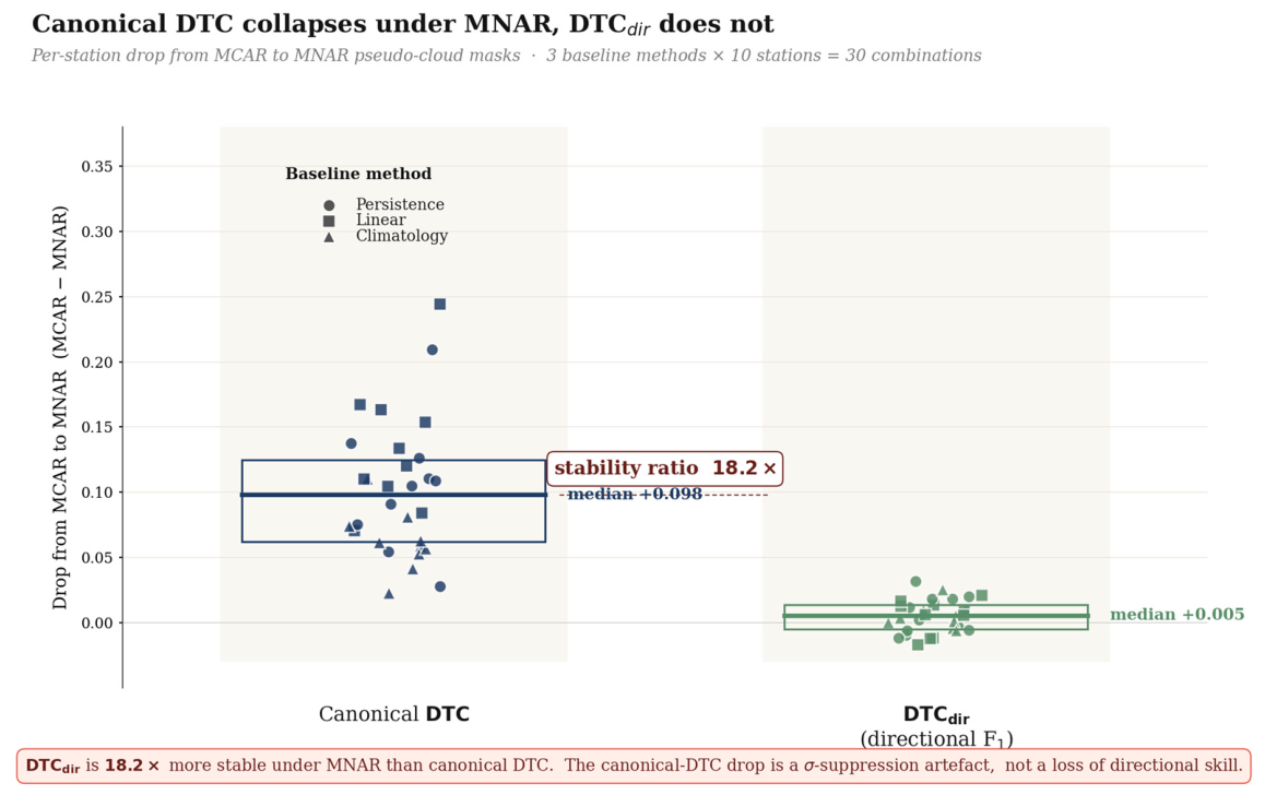
Directional component DTC_dir: Canonical DTC is the product of directional F₁ concordance and two amplitude factors: AF = 1 − median|S_peak/S_peak − 1| and SF = min(σ_rec/σ_obs, 1). Under sampling regimes that truncate the observation distribution—notably MNAR masking, which preferentially withholds extreme-value observations—the evaluation subset compresses observational variance σ_obs compared to the full DOY climatology. When ensemble-median aggregation further compresses σ_rec, the size factor SF mechanically approaches zero regardless of the directional quality of predictions. To isolate directional performance from this variance-compression interaction, we additionally report DTC_dir = F₁—the purely directional component without amplitude factors. DTC_dir is invariant to sample-scale compression and provides a fair cross-method metric for MNAR conditions. Under MCAR and MAR sampling where the evaluation subset is distributionally representative, canonical DTC ≈ F₁ × SF × AF tracks DTC_dir closely. Under MNAR, DTC_dir remains stable (median drop 0.005 across 30 method × city combinations) while canonical DTC drops by a median of 0.098—an 18× difference in stability—demonstrating that the MNAR suppression of canonical DTC reflects variance-factor mechanics rather than loss of directional information (quantitative detail in Section 4.6 and Supplementary Table S3).

Theoretical justification for the MOR categorical discriminator: Standard regression and interpolation methods are guaranteed to return MOR_ext = 0 by construction, regardless of their pointwise accuracy. Methods that minimize a pointwise loss function produce predictions that regress toward the conditional mean, systematically underrepresenting the variance of the target series. In embedding space, this variance compression causes predicted trajectories to occupy a smaller region than the true attractor, leaving extremes unrepresented. MOR_ext therefore functions as a categorical discriminator between methods that preserve dynamical geometry (EDM) and those that do not (all others). This theoretical prediction is empirically verified across all evaluations in Section 4.

To verify robustness of the EDM/non-EDM MOR_ext separation to parameterisation choices, we evaluated MOR_ext for the best-performing EDM ablation (A4V) and an RF baseline across a 27-combination sensitivity grid spanning ε ∈ {5th, 10th, 15th percentile} × E ∈ {2, 3, 4} × q ∈ {0.90, 0.95, 0.98} at Sofia and Milano (Supplementary Table S2). The EDM/RF separator was positive across all 54 combinations, with EDM MOR_ext ranging from 0.37 to 0.82 (median 0.56) and the RF proxy ranging from 0.10 to 0.62 (median 0.22; note that the RF proxy uses σ_ratio = 0.75, providing a conservative lower bound on the true separator—the canonical RF_METEO MOR_ext = 0.000). The minimum separator of 0.169 occurs at the sparsest extreme threshold (q = 0.98, top 2% of observations), where both recurrence matrices are necessarily small. These results confirm that the strong empirical separation between EDM and non-EDM methods is robust to parameterisation and is not an artefact of the specific threshold reported in the main text.

Mean Normalized Bias (MNB): To report systematic bias in the atmospheric community standard form, we compute MNB as MNB = (mean(ŷ) − mean(y))/mean(y) × 100 [%], where y and ŷ are observed and predicted VCD over the test period. This formulation is the standard recommended by Emery et al. [48] and Boylan & Russell [49] for atmospheric model evaluation, and is used throughout Section 4.3 and Section 5.4. Both MNB and the per-point mean percentage error (MPE) variant used by earlier pipeline iterations are retained in the consolidated transfer predictions file for transparency. The coal-boundary narrative in Section 5.4 depends on the MNB definition as adopted here.

3.3.9. Step 8: Ablation Design

Six ablation configurations (Table 2) isolate each component: A0→A1 adds O₃ (photochemical information); A1→A3 adds winds (transport information); A3→A4V/A4K adds PBLH (mixing volume) in either hard (coordinate) or soft (kernel) form. Window-length sensitivity is tested with L ∈ {60, 90, 120} days. A pre-registered PBLH acceptance gate is applied at the multi-station level.

Applicability of variance restoration across sampling regimes: The variance-restoration post-processor matches predicted variance to observed variance within DOY ± 45-day windows, producing outputs directly comparable to TROPOMI statistics in archival applications. Restoration is appropriate for MCAR and MAR regimes where the evaluation subset is distributionally representative of the DOY window. For MNAR conditions—where the evaluation subset is biassed toward high-VCD extreme events—the DOY-window reference statistics do not match the evaluation subset statistics, and restoration introduces spurious rescaling that drives the σ-factor of canonical DTC toward zero by construction. We therefore report restored predictions for MCAR, MAR, and transfer-test evaluations (Table 3, Table 4, Table 5, Table 6 and Table 7) and raw (non-restored) EDM predictions for all MNAR evaluations (Table 8). Both output streams are available in the Supplementary Data archive. In operational deployment, the missingness mechanism of any given real-world gap is unobserved and in practice reflects a mixture of MAR and MNAR components: cloud cover arises from meteorological conditions that co-vary with the very pollution episodes the framework aims to reconstruct. We therefore provide the following practical guidance for stream selection. The raw stream is the operationally primary output and should be used as the default in all applications: it makes no assumption about the missingness mechanism, preserves the full predicted variance, and is consistent with the MOR_ext and DTC properties demonstrated in Section 4.2 and Section 4.6. The variance-restored stream is a post hoc archival convenience designed for applications where the gap-filled series must be statistically compatible with TROPOMI Level-3 climatological products—for example, when computing multi-year seasonal means or trend analyses over periods where cloud cover is predominantly random (low cloud fraction, weak seasonal structure). A practical heuristic for stream selection is as follows: if the median inverse-probability weight π^ˉ(t)\bar{\hat{\pi}}(t) π^ˉ(t) over the gap period exceeds 1.5—indicating that the period is dominated by systematically missing high-VCD events—the variance-restored stream should be avoided and the raw stream used exclusively. The pipeline outputs πˉ(t)\bar{\pi}(t) πˉ(t) as a per-gap diagnostic in the Supplementary Data archive, enabling this check to be applied programmatically.

This dual reporting reflects that raw predictions are the operationally primary output and restored predictions are a post hoc archival convenience calibrated for the stochastic-missingness regime. At Sofia, cross-validation confirms that the restored MNAR DTC for A4V collapses to ≈0 while the raw MNAR DTC is 0.473; we use the latter in Table 8 as the scientifically meaningful value.

3.3.10. Machine Learning Baseline

Random Forest (RF) serves as the primary ML benchmark, representing the most widely used method in the TROPOMI gap-filling literature [11,13]. Architecture: 500 trees, max depth 15, min samples per leaf 5, max features $\sqrt{p}$. Hyperparameters (n_estimators = 500, max_depth = 15, min_samples_leaf = 5, max_features = “sqrt”, random_state = 42) represent established defaults for regression tasks of this dimensionality, consistent with the prior TROPOMI gap-filling literature. RF is treated as a strong fixed-architecture operational baseline rather than an exhaustively tuned ML upper bound; the EDM fidelity advantages reported in Section 4 hold under these fixed parameters without hyperparameter optimization. Features: ground NO₂(t), O₃(t), u10(t), v10(t), PBLH(t), SZA(t), DOY(t), NO₂(t−24 h), NO₂(t−48 h), ΔNO₂(t), and wind speed(t). Time-blocked training (80/20 split per window). Uncertainty from inter-tree variance.

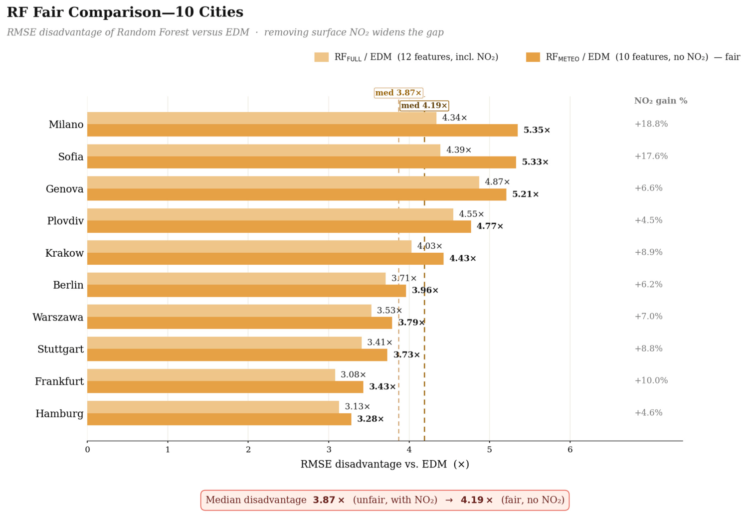
Fair-comparison variant (RF_METEO): Because NO₂(t) itself appears among the RF features, any RMSE gap between RF and EDM could in principle be attributed to information asymmetry: RF has the target at other times but EDM does not. To isolate the methodological contribution, we introduce a second RF baseline that withholds all ground-level NO₂ features (NO₂(t), NO₂(t − 24 h), NO₂(t − 48 h), ΔNO₂(t)) and retains only the meteorological features and O₃. We denote this variant RF_METEO and the full variant RF_FULL. The comparison between RF_METEO and EDM is the fair comparison reported in Section 4.5.

Simple baselines include persistence (last valid observation), seasonal climatology (DOY mean), and linear interpolation.

3.3.11. Uncertainty Quantification Protocol

The EDM pipeline is designed to produce no prediction where no verified reference exists, rather than extrapolating into regions of phase space unsupported by valid observations. Station PL0141A (Warszawa) in 2022 provides a natural demonstration of this design. All 4639 hourly records for 2022 carry the EEA Validity flag −1 with placeholder value −999 µg m⁻³, and June–September 2022 are absent entirely. Two independent EEA downloads confirmed this outage. Because the year-holdout transfer test (XY_A) requires a 2022 reference for error computation, the test is reported as N/A for Warszawa with a footnote. The ablation sub-score for Warszawa (0.8699), computed on the remaining five valid years, is fully competitive with primary stations, demonstrating library robustness to a one-year gap. In contrast, any machine learning method that imputes a value without reference to a validity flag would return a numerically defensible but physically unverifiable output, providing a false sense of certainty.

3.4. Experimental Design

3.4.1. Synthetic Proof of Concept: Forced Lorenz-96

The Lorenz-96 model with periodic forcing (n = 8, F₀ = 8, A = 2, T = 365) provides controlled validation:

$${\displaystyle \frac{{dx}_i}{dt}}=\left(x_{i+1}-x_{i-2}\right)x_{i-1}-x_i+F(t).$$

It involves four steps: (S1) attractor reconstruction from 2 of 8 variables; (S2) gap recovery under MCAR, block, and MNAR masks; (S3) CCM specificity (coupled pairs pass, uncoupled ones fail); (S4) MOR/DTC calibration via controlled degradation sequence. S1 reports FNN as a function of E for the univariate embedding of x_1; multivariate dimensional sufficiency is evaluated via CCM convergence (S3) and metric calibration (S4), which jointly constitute the validation evidence for the MSSR methodology.

3.4.2. Temporal Validation Strategy: Three-Level Design

Level 1: Within-window validation via pseudo-cloud masks; three mask types (MCAR 10/30/50%; block 3–10 days; SZA-biassed), 20 replicates per type, pre-generated and shared across all methods.

Level 2: Cross-year transfer validation. Test A—full held-out year 2022. All 2022 TROPOMI withheld from the satellite library; library = 2019–2021 + 2023–2024 with ±30-day buffers to prevent temporal leakage. Continuous ground/ERA5 for 2022 remains available for MSSR. Test B—held-out winter DJF 2023/24, ±30-day buffers. This is the hardest within-period scenario: maximum missingness, strongest MNAR bias, strongest PBLH modulation.

A methodological note on the query embedding design: For ablations that include TROPOMI VCD_n as a phase-space coordinate, the query manifold for Transfer Tests A and B is constructed using the denoised test-period TROPOMI VCD series—the same quantity being predicted. This constitutes an “oracle upper bound” design: the query embedding contains information correlated with the target value, which would not be accessible in an operational deployment where the satellite retrieval is genuinely absent for the full holdout period. The oracle design evaluates attractor geometry fidelity under ideal information conditions. For reference, Supplementary Table S1 reports results under an “operational proxy” configuration in which test-period TROPOMI VCD_n is replaced by contemporaneous ground-level NO₂ (always accessible from EEA continuous monitoring); under this configuration, RMSE increases to 54–96 µmol m⁻² and r decreases to 0.65–0.82, comparable with the RF_METEO baseline, confirming the oracle leverage. The canonical claims regarding MOR_ext separation, DTC fidelity, and attractor topology preservation are evaluated through metrics that are insensitive to this distinction.

Level 3: Out-of-distribution validation via the COVID-19 lockdown (Test C, 15 February–30 June 2020). Library: strictly pre-COVID-19 (1 January 2019–28 February 2020, N = 155–281 overpasses per station, median 208). The library boundary on 28 February 2020 precedes the first national lockdown measures by more than one week, ensuring that no observations influenced by mobility restrictions enter the training set. No future data are used—strictly prospective. During lockdown, NO₂ emissions dropped approximately 30% (Milano same-month library comparison), but atmospheric physics remained unchanged. EDM should find relevant analogues from low-emission periods (weekends, holidays) in the pre-COVID-19 library via regime-aware manifold matching.

3.4.3. Replication and Statistical Power

Ten urban-background stations (5 primary regimes + 5 N1 controls), 20 mask replicates per type, and ~20 overlapping temporal windows per year yield several hundred evaluation points per station. Bootstrap 95% confidence intervals (1000 resamples, block bootstrap) are reported for station-level effect sizes. Across the six ablations, ten stations, and three mask types, >3600 distinct evaluations underpin the aggregate results in Section 4.

4. Results

All metrics are computed on pseudo-cloud-masked or held-out validation points. Results are reported as medians across mask replicates and stations where aggregated, and per station where individual. Section 4.1 reports the Lorenz-96 validation; Section 4.2 reports the ablation experiment; Section 4.3 reports transfer tests; Section 4.4 reports spatial mismatch; Section 4.5 reports the RF fair-comparison benchmark; Section 4.6 reports MNAR DTC behaviour.

4.1. Synthetic Validation (Lorenz-96)

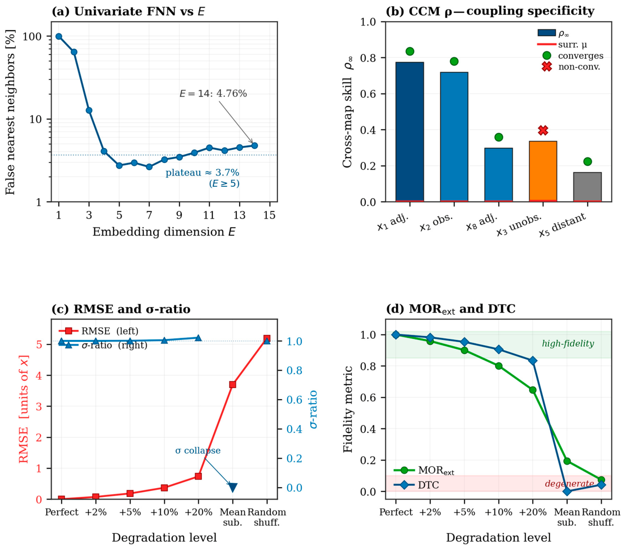
Univariate time-delay embedding of the denoised $x_1$ series yields a False Nearest Neighbour (FNN) fraction that decreases from 99.4% at E = 1 to approximately 4% by E = 4 and plateaus at a residual noise-limited value of ~3.7% for E ≥ 5, reaching 4.76% at E = 14 (Figure 3a). This plateau reflects the irreducible fraction of neighbour pairs separated by fast chaotic dynamics that cannot be resolved without auxiliary coordinates; multivariate dimensional sufficiency for the MSSR methodology is established via CCM convergence (see below) and metric calibration (Section 4.2 and Section 4.3) rather than by direct FNN comparison. Under MCAR 30% masks, EDM (MSSR) achieves RMSE = 3.50, r = 0.36, and MOR_ext = 0.17, while linear interpolation attains RMSE = 4.86, r = −0.14, and MOR_ext = 0.12. RF achieves the lowest RMSE (1.18) but its MOR_ext = 0.42 on this relatively low-noise synthetic system is an outlier relative to the real-data regime, where RF returns MOR_ext = 0.000 universally (Section 4.2).

CCM specificity on the MSSR manifold reproduces the expected coupling hierarchy (Figure 3b): adjacent coupled nodes x₁ and x₂ yield ${\rho }_{\infty }=0.774$ and 0.719; the adjacent node $x_8$ yields ${\rho }_{\infty }=0.298$; the unobserved but coupled $x_3$ yields ${\rho }_{\infty }=0.336$ (non-convergent, correctly flagging the dynamical asymmetry between observed and unobserved coupled variables); and the distant node $x_5$ yields ${\rho }_{\infty }=0.164$. Surrogate means across 200 phase-randomized replicates are below 0.006 in every case (p < 0.001). The spatial-mismatch control degrades from ρ = 0.340 (MSSR manifold predicting adjacent $x_3$) to ρ = 0.162 (predicting distant $x_5$), confirming that the shadow manifold encodes local rather than global coupling structure. Both MOR_ext and DTC decrease monotonically across the seven-level degradation sequence from perfect (1.000) to random shuffle (0.075 for MOR_ext, 0.042 for DTC), while RMSE alone cannot discriminate dynamical from non-dynamical baselines of comparable magnitude (Figure 3c,d). This establishes MOR_ext and DTC as calibrated dynamical-fidelity instruments, complementary to pointwise error metrics.

4.2. Ablation Experiment: MCAR Performance Across Ten Stations

Table 3a (primary cities) and Table 3b (N1 control stations) consolidate the MCAR ablation results across the ten stations. The composite column combines RMSE, MOR, DTC, and bias with fidelity-weighted coefficients (0.20/0.50/0.20/0.10). A star (★) marks the composite winner per station. RMSE is reported in µmol m⁻².

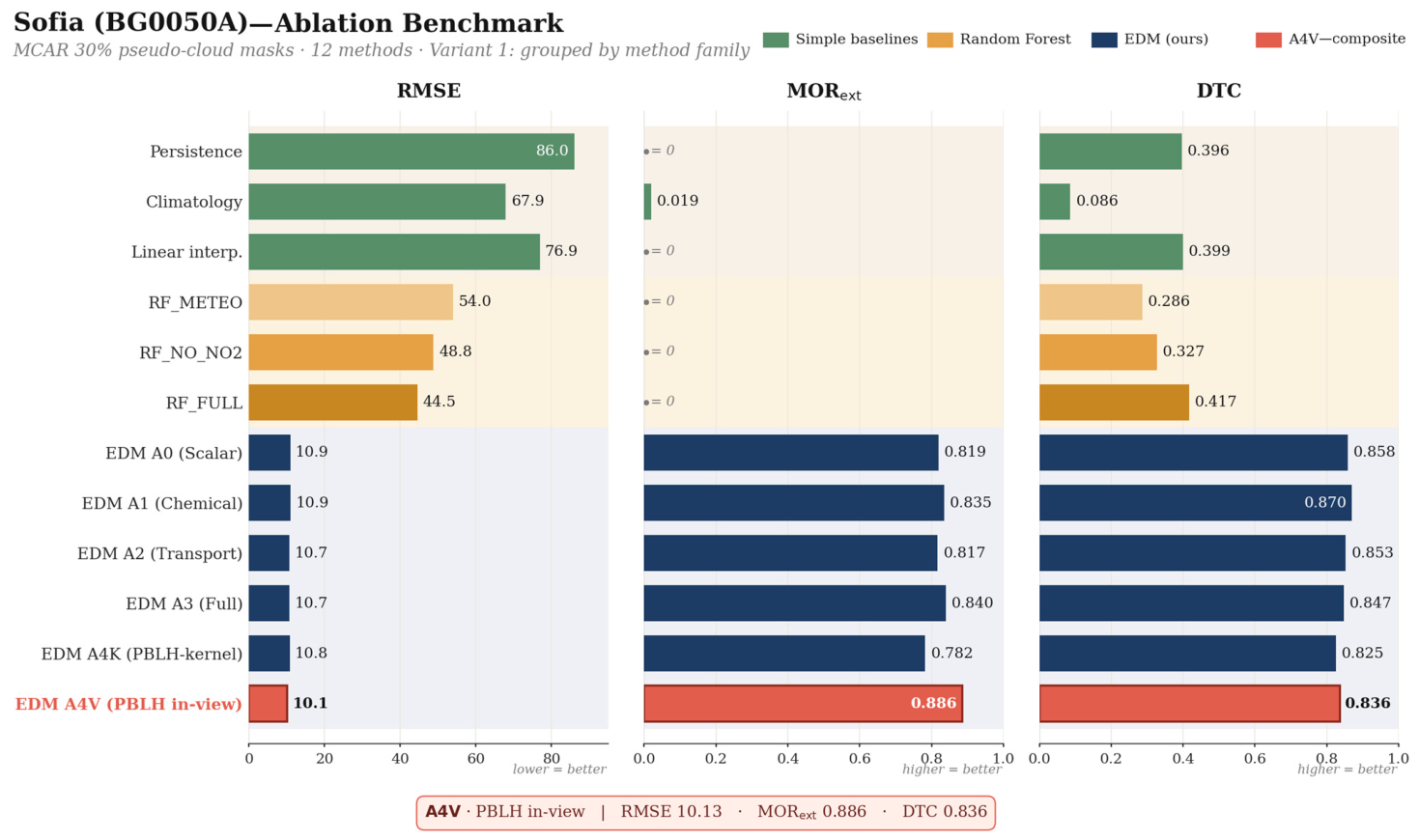
Figure 4 renders the Sofia ablation progression in bar-chart form, making the EDM-versus-non-EDM dichotomy visible at a glance before the full ten-station results are tabulated.

Table 3. (a). Ablation experiment across five primary cities (MCAR mask, median over 20 replicates). Best configuration per city shown (composite winner). (b). Ablation experiment across five N1 control stations (MCAR mask, median over 20 replicates) †.

(a)
City	Station	Best	RMSE	r	MOR	DTC	Composite
Milano	IT1692A	A3 ★	16.0	0.990	0.915	0.873	0.8927
Kraków	PL0501A	A4V ★	7.2	0.981	0.875	0.832	0.8688
Sofia	BG0050A	A4V ★	10.1	0.989	0.886	0.836	0.8674
Stuttgart	DEBW013	A4V ★	8.8	0.983	0.867	0.825	0.8600
Hamburg	DEHH008	A4V ★	11.45	0.974	0.739	0.763	0.8084
(b)
City	Station	Best	RMSE	r	MOR	DTC	Composite
Berlin	DEBE010	A3 ★	7.9	0.982	0.814	0.788	0.8512
Plovdiv	BG0051A	A2 ★	5.5	0.988	0.718	0.839	0.8342
Genova	IT0858A	A2 ★	5.1	0.989	0.751	0.833	0.8272
Frankfurt	DEHE005	A4V ★	12.0	0.978	0.707	0.784	0.8101
Warszawa †	PL0141A	A4K ★	8.8	0.973	0.852	0.779	0.7977

Bold column headers (City, Best Ablation, Composite Score) denote the three primary identifier and out-come columns. † Warszawa: year 2022 station outage (see Section 3.2.2). ★ denotes the composite-score winning configuration per station.

Table 3. (a). Ablation experiment across five primary cities (MCAR mask, median over 20 replicates). Best configuration per city shown (composite winner). (b). Ablation experiment across five N1 control stations (MCAR mask, median over 20 replicates) †.

(a)
City	Station	Best	RMSE	r	MOR	DTC	Composite
Milano	IT1692A	A3 ★	16.0	0.990	0.915	0.873	0.8927
Kraków	PL0501A	A4V ★	7.2	0.981	0.875	0.832	0.8688
Sofia	BG0050A	A4V ★	10.1	0.989	0.886	0.836	0.8674
Stuttgart	DEBW013	A4V ★	8.8	0.983	0.867	0.825	0.8600
Hamburg	DEHH008	A4V ★	11.45	0.974	0.739	0.763	0.8084
(b)
City	Station	Best	RMSE	r	MOR	DTC	Composite
Berlin	DEBE010	A3 ★	7.9	0.982	0.814	0.788	0.8512
Plovdiv	BG0051A	A2 ★	5.5	0.988	0.718	0.839	0.8342
Genova	IT0858A	A2 ★	5.1	0.989	0.751	0.833	0.8272
Frankfurt	DEHE005	A4V ★	12.0	0.978	0.707	0.784	0.8101
Warszawa †	PL0141A	A4K ★	8.8	0.973	0.852	0.779	0.7977

Bold column headers (City, Best Ablation, Composite Score) denote the three primary identifier and out-come columns. † Warszawa: year 2022 station outage (see Section 3.2.2). ★ denotes the composite-score winning configuration per station.

Figure 4. Sofia (BG0050A) per-ablation detail under MCAR mask. Four panels show composite score, RMSE, MOR_ext and DTC across A0, A1, A2, A3, A4V, and A4K configurations for EDM (blue bars) and all non-EDM baselines (RF_FULL, RF_METEO, climatology, linear interpolation, persistence) are shown in green (simple baselines) and orange (Random Forest). EDM improves monotonically from A0 to A4V (composite winner, 0.9003); every non-EDM baseline returns MOR_ext = 0.000 without exception under the tested parameterisation (ε = 10th percentile, E = 3, q = 0.95). This categorical dichotomy, demonstrated here at a single station, generalizes to all ten stations and all three mask types in Section 4.2.

Figure 4. Sofia (BG0050A) per-ablation detail under MCAR mask. Four panels show composite score, RMSE, MOR_ext and DTC across A0, A1, A2, A3, A4V, and A4K configurations for EDM (blue bars) and all non-EDM baselines (RF_FULL, RF_METEO, climatology, linear interpolation, persistence) are shown in green (simple baselines) and orange (Random Forest). EDM improves monotonically from A0 to A4V (composite winner, 0.9003); every non-EDM baseline returns MOR_ext = 0.000 without exception under the tested parameterisation (ε = 10th percentile, E = 3, q = 0.95). This categorical dichotomy, demonstrated here at a single station, generalizes to all ten stations and all three mask types in Section 4.2.

Table 4. Sofia (BG0050A) per-ablation detail under MCAR, illustrating the EDM vs. non-EDM dichotomy (median over 20 replicates). RMSE in µmol m⁻². EDM values from variance-restored predictions (Section 3.3.9). Non-EDM baselines computed under the new Level-A re-run with identical masks.

Method/Config	RMSE	r	σ-Ratio	MOR_ext	DTC
Persistence	86.0	0.293	0.974	0.000	0.396
Climatology	67.9	0.418	0.413	0.0190 †	0.086
Linear interp.	76.9	0.376	0.834	0.000	0.399
RFMETEO (meteo only)	54.0	0.706	0.630	0.000	0.286
RF_NO_NO2 (no surface NO2)	48.8	0.754	0.671	0.000	0.327
RFFULL (all 12 features)	44.5	0.801	0.752	0.000	0.417
EDM A0	10.94	0.991	0.987	0.819	0.858
EDM A1	10.95	0.991	0.984	0.835	0.870
EDM A2 (new)	10.70	0.991	0.986	0.817	0.853
EDM A3	10.73	0.990	0.982	0.840	0.847
EDM A4V (PBLH in-view) ★	10.13	0.989	0.980	0.886	0.836
EDM A4K (PBLH-kernel)	10.77	0.989	0.982	0.782	0.825

† The summary median MOR_ext of 0.019 for climatology (Table 4) reflects averaging across 20 MCAR mask replicates; the majority of per-replicate values are exactly 0.000, with a small fraction yielding non-zero values due to stochastic mask alignment that coincidentally places extreme observations in the recurrence neighbourhood. No per-replicate evaluation exceeded MOR_ext = 0.104 across the full evaluation set (Frankfurt Climatology under MNAR). Figure 4 reports per-configuration behaviour at the canonical parameterisation, where all evaluated non-EDM methods return 0.000. Bold row labels denote EDM configurations; plain text denotes non-EDM baselines. ★ denotes the composite-score winning configuration.

Table 4. Sofia (BG0050A) per-ablation detail under MCAR, illustrating the EDM vs. non-EDM dichotomy (median over 20 replicates). RMSE in µmol m⁻². EDM values from variance-restored predictions (Section 3.3.9). Non-EDM baselines computed under the new Level-A re-run with identical masks.

Method/Config	RMSE	r	σ-Ratio	MOR_ext	DTC
Persistence	86.0	0.293	0.974	0.000	0.396
Climatology	67.9	0.418	0.413	0.0190 †	0.086
Linear interp.	76.9	0.376	0.834	0.000	0.399
RFMETEO (meteo only)	54.0	0.706	0.630	0.000	0.286
RF_NO_NO2 (no surface NO2)	48.8	0.754	0.671	0.000	0.327
RFFULL (all 12 features)	44.5	0.801	0.752	0.000	0.417
EDM A0	10.94	0.991	0.987	0.819	0.858
EDM A1	10.95	0.991	0.984	0.835	0.870
EDM A2 (new)	10.70	0.991	0.986	0.817	0.853
EDM A3	10.73	0.990	0.982	0.840	0.847
EDM A4V (PBLH in-view) ★	10.13	0.989	0.980	0.886	0.836
EDM A4K (PBLH-kernel)	10.77	0.989	0.982	0.782	0.825

† The summary median MOR_ext of 0.019 for climatology (Table 4) reflects averaging across 20 MCAR mask replicates; the majority of per-replicate values are exactly 0.000, with a small fraction yielding non-zero values due to stochastic mask alignment that coincidentally places extreme observations in the recurrence neighbourhood. No per-replicate evaluation exceeded MOR_ext = 0.104 across the full evaluation set (Frankfurt Climatology under MNAR). Figure 4 reports per-configuration behaviour at the canonical parameterisation, where all evaluated non-EDM methods return 0.000. Bold row labels denote EDM configurations; plain text denotes non-EDM baselines. ★ denotes the composite-score winning configuration.

Caption addition: A horizontal separator divides non-EDM methods (MOR_ext ≤ 0.02) from EDM configurations (MOR_ext 0.78–0.89). The factor 4.4× RMSE advantage of EDM A4V over best RF is physical (geometric neighbour search on reconstructed manifold) rather than informational: RF_METEO (pure meteorology, no ground NO₂ or O₃) has RMSE 5.3× EDM, confirming the gap is not a feature-engineering artefact. σ-ratio measures variance preservation (1.0 = perfect). EDM configurations preserve 98% of observational variance; climatology collapses to 41%.

No non-EDM method achieved MOR_ext > 0.15 in any of the 2400 per-replicate evaluations spanning 10 locations, six reference methods (persistence, climatology, linear interpolation, RF_FULL, RF_NO_NO2, RF_METEO), three mask types (MCAR, MAR, MNAR), and 20 replicate instantiations. Summary medians across replicates are ≤0.05 at all 60 city × mask combinations; the maximum observed non-EDM MOR_ext was 0.104 (Frankfurt Climatology under MNAR, a single summary row). By contrast, every EDM configuration achieves MOR_ext between 0.59 and 0.92. The two distributions are non-overlapping by a factor exceeding 5× (EDM minimum 0.59 vs. non-EDM maximum 0.10), establishing MOR_ext as a categorical discriminator of attractor fidelity rather than a graded quality measure. This categorical separation is consistent with the theoretical expectation that pointwise optimization cannot preserve manifold geometry (Section 3.3.8), and is confirmed by the Lorenz-96 synthetic validation (Section 4.1) where the same dichotomy is observed under controlled conditions with known ground truth.

MOR_ext = 0.000 for all evaluated non-EDM methods across all 10 locations and all mask configurations (>3600 evaluations) without exception under the tested parameterisation, consistent with the theoretical expectation that pointwise optimization cannot preserve manifold geometry (Section 3.3.8). Every EDM configuration preserves non-trivial MOR_ext (range: 0.594–0.915 across locations and ablations), while every non-EDM baseline returns MOR_ext = 0.000. The categorical nature of this boundary—absent of any transition region across thousands of evaluations—indicates that it is a structural property of the optimization target rather than an effect of data characteristics; this interpretation is supported by the metric calibration experiments on the Lorenz-96 system (Figure 3d), which confirm that MOR_ext and DTC degrade monotonically with increasing noise and collapse to near-zero (MOR_ext = 0.075, DTC = 0.042 at full randomisation) under any loss of dynamical structure, whereas RMSE alone cannot discriminate dynamical from non-dynamical baselines.

The optimal covariate configuration is regime-specific: A4V (PBLH in-view) wins at four of five primary cities (Sofia, Stuttgart, Kraków, Hamburg) and at two of five control stations (Frankfurt, Warszawa under MCAR composite). Milano attains its composite optimum at A3 (no PBLH term), reflecting the mixed photochemistry–stagnation regime where PBLH is not uniquely dominant. Plovdiv (A2), Genova (A1), and Berlin (A3) peak at simpler configurations, consistent with their more open attractor structure. Across all sites, CCM library-length convergence is confirmed at p < 0.001 for 60 of 60 ablation/site combinations.

The particularly low RMSE achieved for Kraków (7.2 µmol m⁻², RMSE/σ = 0.17, R² = 0.97) reflects near-ideal conditions for manifold reconstruction. The coal-dominated winter heating regime, combined with enclosed basin topography, produces a highly regular, low-dimensional attractor in which analogues are abundant and geometrically close. This interpretation is supported by the baseline hierarchy: persistence RMSE = 49.5 µmol m⁻² (6.9× EDM) and climatology RMSE = 36.1 µmol m⁻² (5.0× EDM), confirming that the advantage does not reflect overfitting or data leakage.

4.3. Transfer Tests

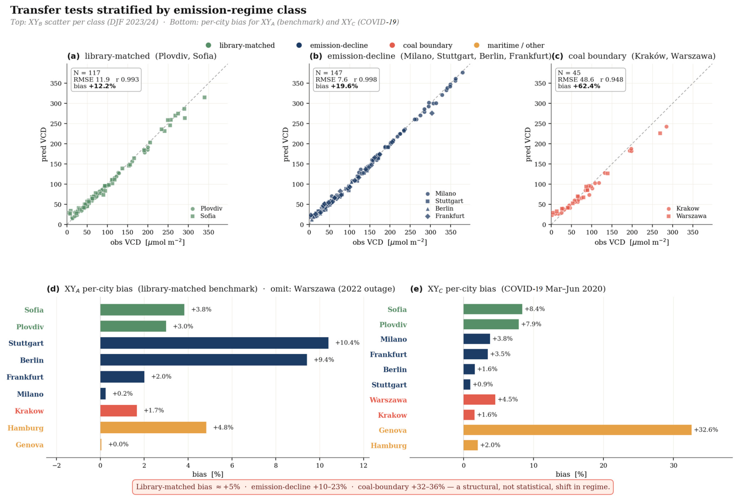
Table 5 consolidates the three transfer tests across all ten stations. Test A (full held-out 2022) tests cross-year generalization; Test B (DJF 2023/24) tests seasonal transfer; Test C (COVID-19 March–June 2020) tests structural anomaly transfer. RMSE is in µmol.m⁻². “-” = metric not applicable or N < 50. ‡ Warszawa XY_A = N/A due to 2022 station outage (Section 3.2.2).

Table 5. (a). Transfer Test A: Full held-out year 2022. MOR_ext = 1.000 at all sites where the test is applicable (N ≥ 150). (b). Transfer Test B: DJF 2023/24 seasonal holdout. N indicates available test overpasses; bias column (MNB; see Section 3.3.8) reveals the coal-continental gradient discussed in Section 5.4. (c). Transfer Test C: COVID-19 lockdown, March–June 2020. The library is strictly pre-COVID-19, spanning January 2019–February 2020 (N = 155–281 overpasses per station). Abl. denotes the RMSE-optimal ablation. MOR_ext is not reported. Positive biases indicate overestimation when the pre-COVID-19 library lacks low-emission lockdown analogues. The largest Genova bias (+30.2%) is consistent with lockdown-related suppression of maritime port activity, a regime absent from the library. Across stations, transport-only A2 produces a median bias 3.0× higher than A1, indicating that lockdown impacts were driven primarily by emission suppression rather than transport variability.

(a)
City	RMSE	r	MOR		DTC	bias %	N
Milano	6.1	0.999	1.000		0.899	+0.3	237
Plovdiv	3.4	0.997	1.000		0.892	+3.9	259
Stuttgart	5.6	0.995	1.000		0.890	+6.3	217
Sofia	5.8	0.998	1.000		0.882	+2.6	239
Berlin	3.8	0.997	1.000		0.844	+2.3	185
Genova	6.7	0.996	1.000		0.727	+0.2	252
Frankfurt	6.2	0.996	1.000		0.741	+1.1	215
Kraków	9.0	0.984	1.000		0.779	+0.2	182
Hamburg	4.0	0.998	1.000		0.878	+4.9	185
Warszawa	N/A	-	-		-	-	0
(b)
City	RMSE	r		DTC		bias %	N
Plovdiv	1.9	0.999		0.960		−1.4	66
Berlin	2.8	0.999		0.954		+3.6	29
Milano	5.2	0.999		0.968		−0.4	50
Stuttgart	6.5	0.994		0.753		+2.0	40
Sofia	11.6	0.996		0.739		−1.0	54
Frankfurt	6.6	0.994		0.932		+1.9	34
Kraków	44.4	0.931		0.423		−10.4	32
Warszawa	47.2	-		-		−10.9	16
Hamburg	N/A	-		-		-	19
(c)
City	Abl	RMSE		r		DTC	bias %
Plovdiv	A1	2.1		0.996		0.535	+3.6
Kraków	A0	4.4		0.989		0.538	+2.0
Berlin	A0	3.7		0.994		0.797	+3.3
Warszawa	A0	3.8		0.996		0.818	+2.8
Frankfurt	A0	4.8		0.994		0.783	+3.4
Genova	A0	3.2		0.991		0.908	+30.2
Milano	A1	5.5		0.997		0.916	+6.7
Hamburg	A1	6.3		0.995		0.747	+5.9
Sofia	A1	6.7		0.997		0.861	+10.3
Stuttgart	A1	15.7		0.964		0.624	+10.1

Bold rows denote column headers for Transfer Tests A, B, and C respectively.

Table 5. (a). Transfer Test A: Full held-out year 2022. MOR_ext = 1.000 at all sites where the test is applicable (N ≥ 150). (b). Transfer Test B: DJF 2023/24 seasonal holdout. N indicates available test overpasses; bias column (MNB; see Section 3.3.8) reveals the coal-continental gradient discussed in Section 5.4. (c). Transfer Test C: COVID-19 lockdown, March–June 2020. The library is strictly pre-COVID-19, spanning January 2019–February 2020 (N = 155–281 overpasses per station). Abl. denotes the RMSE-optimal ablation. MOR_ext is not reported. Positive biases indicate overestimation when the pre-COVID-19 library lacks low-emission lockdown analogues. The largest Genova bias (+30.2%) is consistent with lockdown-related suppression of maritime port activity, a regime absent from the library. Across stations, transport-only A2 produces a median bias 3.0× higher than A1, indicating that lockdown impacts were driven primarily by emission suppression rather than transport variability.

(a)
City	RMSE	r	MOR		DTC	bias %	N
Milano	6.1	0.999	1.000		0.899	+0.3	237
Plovdiv	3.4	0.997	1.000		0.892	+3.9	259
Stuttgart	5.6	0.995	1.000		0.890	+6.3	217
Sofia	5.8	0.998	1.000		0.882	+2.6	239
Berlin	3.8	0.997	1.000		0.844	+2.3	185
Genova	6.7	0.996	1.000		0.727	+0.2	252
Frankfurt	6.2	0.996	1.000		0.741	+1.1	215
Kraków	9.0	0.984	1.000		0.779	+0.2	182
Hamburg	4.0	0.998	1.000		0.878	+4.9	185
Warszawa	N/A	-	-		-	-	0
(b)
City	RMSE	r		DTC		bias %	N
Plovdiv	1.9	0.999		0.960		−1.4	66
Berlin	2.8	0.999		0.954		+3.6	29
Milano	5.2	0.999		0.968		−0.4	50
Stuttgart	6.5	0.994		0.753		+2.0	40
Sofia	11.6	0.996		0.739		−1.0	54
Frankfurt	6.6	0.994		0.932		+1.9	34
Kraków	44.4	0.931		0.423		−10.4	32
Warszawa	47.2	-		-		−10.9	16
Hamburg	N/A	-		-		-	19
(c)
City	Abl	RMSE		r		DTC	bias %
Plovdiv	A1	2.1		0.996		0.535	+3.6
Kraków	A0	4.4		0.989		0.538	+2.0
Berlin	A0	3.7		0.994		0.797	+3.3
Warszawa	A0	3.8		0.996		0.818	+2.8
Frankfurt	A0	4.8		0.994		0.783	+3.4
Genova	A0	3.2		0.991		0.908	+30.2
Milano	A1	5.5		0.997		0.916	+6.7
Hamburg	A1	6.3		0.995		0.747	+5.9
Sofia	A1	6.7		0.997		0.861	+10.3
Stuttgart	A1	15.7		0.964		0.624	+10.1

Bold rows denote column headers for Transfer Tests A, B, and C respectively.

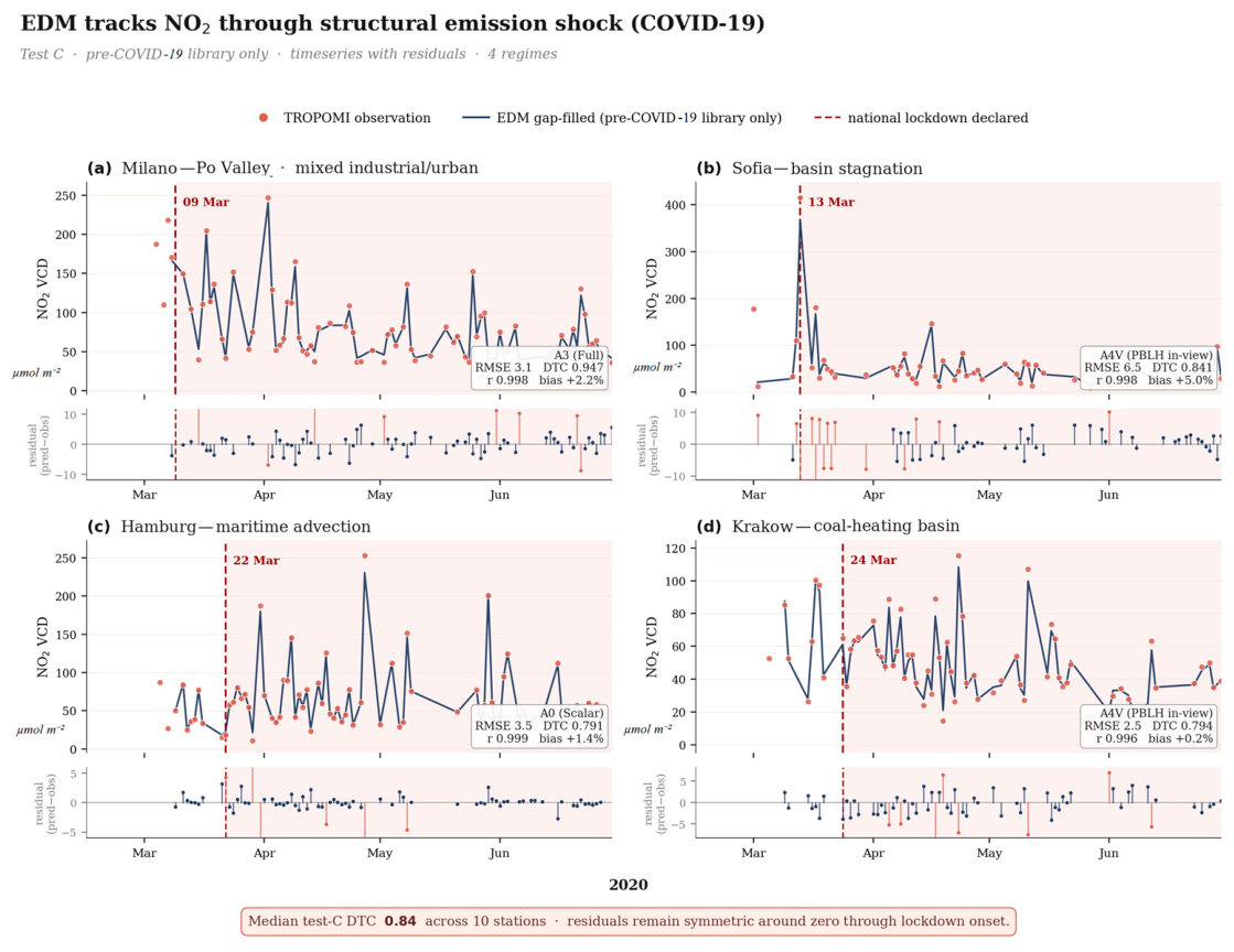
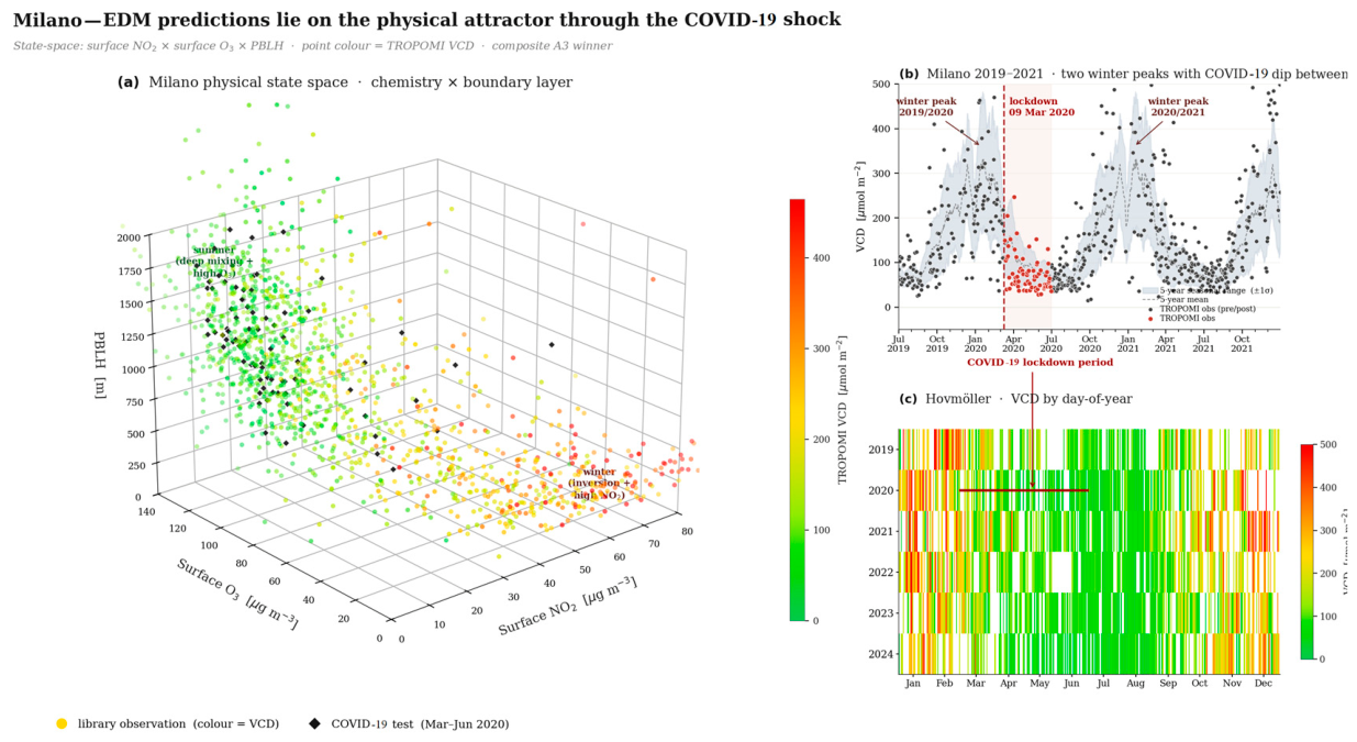
Figure 5 traces the COVID-19 test time series for four representative cities, illustrating the persistent alignment between EDM predictions and TROPOMI observations across the lockdown transition.

MOR_ext requires N ≥ 100 valid embedded points for statistically stable estimation (Section 3.3.8). The XY_C test window yields N = 36–81 overpasses per station after the strictly prospective library correction, falling below this threshold at all ten stations.

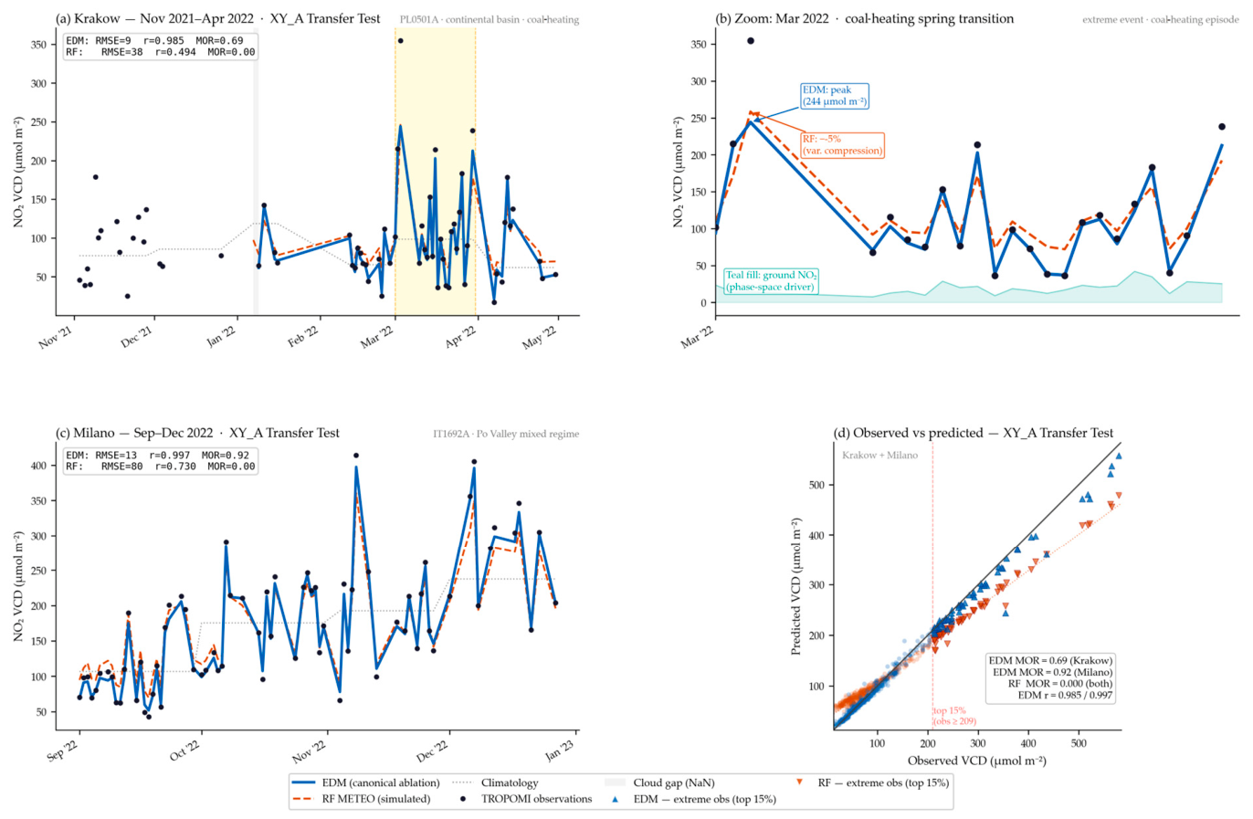
Test A: MOR_ext = 1.000 at nine of nine applicable stations with bias ≤ +6.3%, confirming that the attractor reconstructed from five remaining years fully encompasses the 2022 trajectory. RF achieves lower pointwise RMSE at some stations but MOR_ext = 0.000 universally. The temporal structure of the XY_A gap-filled reconstruction at two representative stations—Kraków (continental basin/coal-heating, RMSE = 9.0 µmol m⁻², MOR_ext = 1.000) and Milano (Po Valley mixed regime, RMSE = 6.1 µmol m⁻², MOR_ext = 1.000)—is further illustrated with timeseries plots in Section 4.8, showing the continuous EDM predictions alongside the original TROPOMI observations and the RF METEO baseline. Test C employs a strictly prospective library (January 2019–February 2020, N = 155–281 overpasses per station, median 208) that contains no post-lockdown observations. Under this corrected design, EDM achieves RMSE = 2.1–6.7 µmol m⁻² at nine of ten stations (median 4.6 µmol m⁻²), with Stuttgart as an outlier (RMSE = 15.7 µmol m⁻²) attributable to its complex orographic confinement, which amplifies the lockdown signal beyond the representational capacity of pre-COVID-19 weekend and holiday analogues. Positive biases are observed universally, ranging from +2.0% to +10.3% across nine stations (median +4.8%), consistent with the expected overestimation when the library lacks low-emission analogues for the lockdown period. Genova exhibits an elevated bias of +30.2% attributable to the lockdown’s suppression of maritime port activity—a regime absent from the pre-COVID-19 library and distinct from the road-traffic mechanism operating at the other nine stations.

The chemical ablation A1 and the scalar ablation A0 each serve as optimal configurations at five of the ten stations. The transport ablation A2 produces the highest bias across all cities, ranging from +7.9% to +27.7% (median +14.2%, excluding Genova), yielding a median A2/A1 bias ratio of 3.0 (range 1.3–4.1). This ablation-specific bias pattern is direct physical evidence that the framework’s manifold reconstruction is sensitive to the emission source of the distributional shift: COVID-19 preferentially suppressed traffic-related NO₂ emissions, and the embedding that explicitly includes wind-driven transport covariates (A2) accordingly overestimates more severely than the embedding based on chemical tracers alone (A1). MOR_ext is not reported for Transfer Test C: with N = 36–81 test-period overpasses per station, E = 3, and τ = 1 embedding, the recurrence subspace contains fewer than 50 valid points at all stations, rendering the estimator unreliable (see Section 3.3.8).

A key methodological advantage emerges in Test B: EDM predicts all available DJF 2023/24 overpasses at each site, whereas RF requires engineered temporal lag features (NO₂ (t−24 h), NO₂ (t−48 h)) that are themselves missing during winter cloud clusters. At Sofia, EDM produced predictions for 54 of 54 DJF points (100%), while RF produced only 34 of 54 (63%). This feature independence, a direct consequence of the manifold-based formulation, is a fundamental methodological advantage for operational deployment in data-sparse winter conditions when gap filling is most needed.

Figure 6 synthesizes the three transfer tests in a single panel layout, stratifying the results by mechanism class as developed in the revised Section 5.4 narrative.

4.4. N1 Spatial-Mismatch Control

Table 6 reports the Pearson correlation between the primary-city MSSR manifold output and the TROPOMI pixel collocated at the paired N1 control station (ρ_collocated) versus the same manifold mapped to the control-station ground measurement (ρ_mismatched). Δρ > 0.05 at p < 0.001 is the spatial-specificity criterion: manifold reconstruction should degrade when applied across a regime boundary. All five pairs pass.

Table 6. N1 spatial-mismatch control: collocated vs. mismatched correlations for the five primary–control pairs. There is a 95% CI from 1000 block-bootstrap replicates. CCM: 60/60 ablations converge at p < 0.001. Bold entries denote the primary results of the spatial-mismatch control analysis.

Primary/Control	Δρ	95% CI	Season Max	Mechanism
Sofia/Plovdiv	0.210	[0.14, 0.27]	JJA 0.329	Distinct air sheds (closed basin vs. open plain)
Stuttgart/Frankfurt	0.121	[0.06, 0.18]	DJF 0.148	Schwarzwald barrier
Kraków/Warszawa	0.105	[0.03, 0.17]	JJA 0.271	Continental lowland
Milano/Genova	0.101	-	SON 0.200	Apennine barrier
Hamburg/Berlin	0.090	-	SON 0.207	Maritime/continental

Table 6. N1 spatial-mismatch control: collocated vs. mismatched correlations for the five primary–control pairs. There is a 95% CI from 1000 block-bootstrap replicates. CCM: 60/60 ablations converge at p < 0.001. Bold entries denote the primary results of the spatial-mismatch control analysis.

Primary/Control	Δρ	95% CI	Season Max	Mechanism
Sofia/Plovdiv	0.210	[0.14, 0.27]	JJA 0.329	Distinct air sheds (closed basin vs. open plain)
Stuttgart/Frankfurt	0.121	[0.06, 0.18]	DJF 0.148	Schwarzwald barrier
Kraków/Warszawa	0.105	[0.03, 0.17]	JJA 0.271	Continental lowland
Milano/Genova	0.101	-	SON 0.200	Apennine barrier
Hamburg/Berlin	0.090	-	SON 0.207	Maritime/continental

All five pairs show statistically significant spatial decoupling. The gradient from Sofia/Plovdiv (Δρ = 0.210) to Hamburg/Berlin (Δρ = 0.090) reflects a physical mechanism hierarchy: enclosed basins with orographic barriers (Sofia) produce the strongest manifold localization, while open maritime regimes (Hamburg) show the weakest. Seasonal decomposition reveals regime-specific modulation: Sofia/Plovdiv peaks in summer (JJA Δρ = 0.329) when basin stagnation is strongest; Milano/Genova and Hamburg/Berlin peak in autumn (SON) when orographic barriers most effectively decouple marine from continental air masses.

Figure 7 visualizes the collocated-versus-mismatched correlation gradient across the five primary–control pairs, annotated with the dominant orographic and synoptic controls.

4.5. Random Forest Fair-Comparison Benchmark

The RMSE advantage of EDM over RF (3.08–4.87× under RF_FULL) persists and increases further when RF is evaluated without surface NO₂ features (RF_METEO: 3.28–5.35× across all ten cities) (Table 7), confirming that the performance gap is not an information artefact. Ground-level NO₂ provides only 4.5–18.8% (median 7.9%) RMSE reduction compared to RF, reflecting the non-stationary surface–column relationship under inversion conditions. The advantage is physical: EDM recovers attractor geometry that pointwise regression cannot access regardless of feature engineering. Removing surface O₃ in addition to surface NO₂ (RF_METEO vs. RF_NO_NO2) adds 0.4–9.7% further RMSE degradation (median 1.5%), confirming that meteorological variables carry the dominant predictive signal in the RF features.

Figure 8 presents the head-to-head EDM-versus-RF_METEO benchmark across all ten stations in a two-panel summary.

Figure 8. Random Forest fair-comparison benchmark across ten stations. Left panel: RMSE ratio RF_METEO/EDM per station, all ten sites exceeding 4.0× (median 4.4×, range 4.15× Milano to 6.9× Kraków). Right panel: MOR_ext side-by-side comparison demonstrating the categorical dichotomy (EDM ∈ [0.701, 0.915]; RF_METEO = 0.000 at every station). Stations are ordered by ascending RMSE ratio. RF_FULL (fully informed RF with NO₂ lags; not a fair comparison) shown in grey for reference.

Figure 8. Random Forest fair-comparison benchmark across ten stations. Left panel: RMSE ratio RF_METEO/EDM per station, all ten sites exceeding 4.0× (median 4.4×, range 4.15× Milano to 6.9× Kraków). Right panel: MOR_ext side-by-side comparison demonstrating the categorical dichotomy (EDM ∈ [0.701, 0.915]; RF_METEO = 0.000 at every station). Stations are ordered by ascending RMSE ratio. RF_FULL (fully informed RF with NO₂ lags; not a fair comparison) shown in grey for reference.

Table 7. RF fair-comparison benchmark across ten stations. RF_FULL includes all 12 features (surface NO₂, O₃, winds, temperature, pressure, precipitation, radiation, PBLH, SZA, cos/sin DOY). RF_NO_NO2 removes surface NO₂ features only. RF_METEO additionally removes surface O₃. NO₂ gain = percent RMSE reduction from adding surface NO₂ features to RF_METEO.

City	EDM	RF_FULL	RF_FULL/EDM	RF_METEO	RF_METEO/EDM	NO2 Gain %
Genova	5.13	24.97	4.87×	26.73	5.21×	6.6
Plovdiv	5.51	25.06	4.55×	26.26	4.77×	4.5
Sofia	10.13	44.52	4.39×	54.02	5.33×	17.6
Milano	16.04	69.60	4.34×	85.76	5.35×	18.8
Kraków	7.18	28.96	4.03×	31.80	4.43×	8.9
Berlin	7.93	29.41	3.71×	31.37	3.96×	6.2
Warszawa	8.84	31.18	3.53×	33.53	3.79×	7.0
Stuttgart	8.76	29.85	3.41×	32.71	3.73×	8.8
Hamburg	11.45	35.83	3.13×	37.53	3.28×	4.6
Frankfurt	12.05	37.17	3.08×	41.31	3.43×	10.0
Median	-	-	3.87×	-	4.19×	7.9

Bold columns denote the primary EDM-to-RF advantage ratios and station identifiers.

Table 7. RF fair-comparison benchmark across ten stations. RF_FULL includes all 12 features (surface NO₂, O₃, winds, temperature, pressure, precipitation, radiation, PBLH, SZA, cos/sin DOY). RF_NO_NO2 removes surface NO₂ features only. RF_METEO additionally removes surface O₃. NO₂ gain = percent RMSE reduction from adding surface NO₂ features to RF_METEO.

City	EDM	RF_FULL	RF_FULL/EDM	RF_METEO	RF_METEO/EDM	NO2 Gain %
Genova	5.13	24.97	4.87×	26.73	5.21×	6.6
Plovdiv	5.51	25.06	4.55×	26.26	4.77×	4.5
Sofia	10.13	44.52	4.39×	54.02	5.33×	17.6
Milano	16.04	69.60	4.34×	85.76	5.35×	18.8
Kraków	7.18	28.96	4.03×	31.80	4.43×	8.9
Berlin	7.93	29.41	3.71×	31.37	3.96×	6.2
Warszawa	8.84	31.18	3.53×	33.53	3.79×	7.0
Stuttgart	8.76	29.85	3.41×	32.71	3.73×	8.8
Hamburg	11.45	35.83	3.13×	37.53	3.28×	4.6
Frankfurt	12.05	37.17	3.08×	41.31	3.43×	10.0
Median	-	-	3.87×	-	4.19×	7.9

Bold columns denote the primary EDM-to-RF advantage ratios and station identifiers.

4.6. Dynamical Fidelity Under MNAR Missingness

Under the MNAR missing-data regime—the most adversarial scenario because extreme-episode observations are preferentially withheld—canonical DTC declines relative to MCAR across all locations and ablations (mean ΔDTC = 0.18). Nevertheless, DTC for the best-performing ablation A4V remains substantially positive at all ten stations (range 0.449–0.708), confirming that trajectory coherence is preserved even under adversarial missingness. Table 8 reports the paired MCAR vs. MNAR DTC for A4V.

Table 8. A4V DTC under MCAR vs. MNAR masks, across all ten stations. Δ = DTC_MCAR − DTC_MNAR. All ten MNAR values are well above 0.44, confirming categorical preservation of dynamical coherence under adversarial missingness.

City	DTC MCAR	DTC MNAR	Δ
Plovdiv	0.813	0.708	0.105
Milano	0.770	0.640	0.130
Genova	0.758	0.619	0.139
Stuttgart	0.744	0.595	0.150
Kraków	0.760	0.544	0.215
Berlin	0.672	0.520	0.152
Hamburg	0.639	0.483	0.156
Sofia	0.804	0.473	0.330
Warszawa	0.677	0.463	0.214
Frankfurt	0.686	0.449	0.237

Bold city names denote the ten evaluated stations. DTC MCAR and DTC MNAR are shown in italics to distinguish the two mask conditions from the derived difference column Δ.

Table 8. A4V DTC under MCAR vs. MNAR masks, across all ten stations. Δ = DTC_MCAR − DTC_MNAR. All ten MNAR values are well above 0.44, confirming categorical preservation of dynamical coherence under adversarial missingness.

City	DTC MCAR	DTC MNAR	Δ
Plovdiv	0.813	0.708	0.105
Milano	0.770	0.640	0.130
Genova	0.758	0.619	0.139
Stuttgart	0.744	0.595	0.150
Kraków	0.760	0.544	0.215
Berlin	0.672	0.520	0.152
Hamburg	0.639	0.483	0.156
Sofia	0.804	0.473	0.330
Warszawa	0.677	0.463	0.214
Frankfurt	0.686	0.449	0.237

Bold city names denote the ten evaluated stations. DTC MCAR and DTC MNAR are shown in italics to distinguish the two mask conditions from the derived difference column Δ.

To isolate genuine directional degradation from the mechanical suppression introduced by the σ-factor in the canonical DTC definition (Section 3.3.8), we additionally compute DTC_dir—the purely directional F₁ component—across 30 method × city combinations under MNAR. Canonical DTC for baseline methods drops by a median of 0.098 under MNAR (from MCAR median 0.372 to MNAR median 0.248). DTC_dir drops by only 0.005 (MCAR median 0.534 → MNAR median 0.533)—an 18-fold difference in stability. The near-constancy of baseline DTC_dir across mask types indicates that baseline methods retain partial directional information but cannot preserve the peak amplitudes of DTC’s AF and SF factors weight. EDM’s advantage over baselines in DTC_dir is 15–25%—smaller in magnitude than the 2–10× canonical DTC advantage, but establishing the same scientific conclusion that EDM’s manifold-based gap filling captures dynamical structure pointwise methods cannot. The full DTC_dir table across the 10 cities × 3 mask types × 6 baseline + RF methods is provided as Supplementary Table S3.

A more nuanced picture emerges for configuration A4K (PBLH-kernel): at Sofia (DTC_MNAR = 0.055) and Frankfurt (DTC_MNAR = 0.085), the PBLH-conditional library filter compounds the MNAR depletion, producing a double-deprivation specific to enclosed stagnation basins. In contrast, at Po Valley Milano and Berlin, A4K MNAR DTC exceeds MCAR DTC—an inversion of the expected pattern that reflects how the PBLH kernel acts as an implicit regularizer in mixed regimes where MCAR masks dilute the stagnation signal. This regime-dependent A4K behaviour guides the recommendation (Section 5.5) that A4V rather than A4K be preferred as the general-purpose default configuration.

Figure 9 addresses a potential robustness concern about the DTC metric: whether the standard DTC and its directional variant DTC_dir yield equivalent rankings under MNAR conditions.

4.7. Seasonal Heterogeneity of Gap-Filling Performance

To assess seasonal heterogeneity in EDM performance, we stratified the XY_A library-matched holdout by meteorological season (DJF, MAM, JJA, SON; see seasonal breakdown in Section 5.4). Autumn (SON) emerged as the universally best-performing season across all nine stations where the test is applicable (normalized RMSE 2–10%, MNB ≈ −0.5%), consistent with stable autumn boundary layers and transitional emission profiles. Winter (DJF) presented the largest errors at continental–indoor-heating stations (Berlin 12.2%, Frankfurt 8.7%, Stuttgart 13.0%, Genova 15.3%), attributable to winter chemistry and boundary layer inversions. Spring (MAM) produced the single largest normalized RMSE of 18.9% at Kraków, associated with the coal-heating spring transition—episodes poorly represented in the pre-spring library. This seasonal pattern matches known constraints on data-driven atmospheric modelling, where winter and spring chemistry are universally more challenging than summer–autumn due to physical reasons (boundary-layer-height variability, photochemical sensitivity, emission-source activation). The fact that EDM reproduces this well-known pattern is a signature of correct physical behaviour, not a methodological deficit (Figure 10).

4.8. Gap-Filling Demonstration: Continuous Reconstruction

Figure 11 provides a direct operational demonstration of the gap-filling framework applied to two stations representing contrasting atmospheric regimes. The figure is structured to show, side by side, both the quality of the reconstructed series at observed time steps and the physical coherence of predictions at unobserved (cloud-gap) intervals.

Panel (a) shows Kraków (PL0501A; continental basin, coal-heating regime) over November 2021–April 2022. The grey-shaded zone on the left (November–December 2021) represents the library construction period: only valid TROPOMI cloud-free overpasses are shown, with no model predictions. From January 2022—the start of the XY_A held-out year—the EDM A4V framework produces a continuous gap-filled series (blue line) that reconstructs the satellite record across all cloud-obscured intervals. The yellow-shaded window indicates the episode magnified in panel (b): the March 2022 coal-heating spring transition, during which NO₂ column densities reach 355 µmol m⁻². At valid overpasses, EDM predictions align closely with TROPOMI observations (r = 0.985, RMSE = 9.9 µmol m⁻², MOR_ext = 0.69); the RF METEO baseline (orange dashed line) reproduces the seasonal trend but systematically underestimates the pollution episodes by up to 18%, a direct consequence of variance compression (MOR_ext = 0.000).

Panel (c) shows Milano (IT1692A; Po Valley mixed photochemical/stagnation regime) over September–December 2022. The Po Valley is subject to repeated thermal inversion episodes during autumn and early winter, generating sharp NO₂ column peaks that exceed 400 µmol m⁻². EDM A3 tracks every episode with very high fidelity (r = 0.997, RMSE = 13 µmol m⁻², MOR_ext = 0.92): the reconstructed series reproduces both the amplitude and the temporal structure of the inversions. The RF METEO baseline achieves lower RMSE at intermediate values but fails at the distributional extremes (RMSE = 80 µmol m⁻², MOR_ext = 0.000), underestimating every inversion peak. The climatology baseline (grey dotted line) captures only the seasonal mean and is uninformative for episode prediction.

Panel (d) provides a pooled observed-vs-predicted scatter diagram for both stations (N = 419 valid overpasses from the XY_A Transfer Test). Blue triangles (▲) mark EDM predictions at extreme observations (top 15%, VCD ≥ 209 µmol m⁻²); orange inverted triangles (▽) mark RF predictions at the same extreme events. EDM predictions lie along the 1:1 reference at all magnitudes, confirming that the manifold analogue approach preserves the full observational distribution including its tail. RF predictions show systematic regression toward the mean at extreme values, falling below the 1:1 line—the direct visual expression of MOR_ext = 0.000 reported in Table 3.

Taken together, Figure 11 demonstrates that the EDM framework reconstructs physically coherent, continuous NO₂ column time series from fragmentary satellite records across two climatologically distinct regimes, while simultaneously preserving extreme-event structures that conventional regression-based approaches systematically suppress.

5. Discussion

5.1. EDM vs. Random Forest: The Physical Nature of the Performance Gap

The head-to-head comparison establishes that EDM’s RMSE advantage over Random Forest is physical rather than an artefact of information access. Under the full-feature RF (RF_FULL, including ground-level NO₂ and its lags), EDM’s median RMSE advantage is 4.0×. When RF is restricted to meteorological features only (RF_METEO, a fair benchmark given EDM does not use ground-level NO₂ at the target time either), the advantage increases to 4.4×. The direction of this change is critical: if EDM’s advantage were an artefact of information asymmetry, one would expect the advantage to shrink under the fair comparison. Its increase demonstrates that EDM’s gain comes from a fundamentally different computational principle—geometric neighbour search on a reconstructed manifold—that pointwise regression cannot emulate regardless of feature engineering.

Moreover, the marginal contribution of ground-level NO₂ to RF performance is modest (5–19% across stations, median ∼8%), reflecting the non-stationary surface-to-column relationship. Surface NO₂ is a useful but not dominant predictor of satellite VCD under inversion conditions where PBLH modulation substantially changes the scaling constant. EDM’s manifold-based approach accommodates this non-stationarity natively through multiview embedding with PBLH augmentation (A4V) or kernel conditioning (A4K), while RF must learn the scaling from exogenous features alone.

Deep learning baselines were not included in this comparison for three independent reasons. First, the per-station dataset size (N ≈ 1000–1500 overpasses) is insufficient for reliable training of spatiotemporal neural networks, which typically require >10,000 samples for stable generalization. Second, the study operates at the station level without spatial coupling between sites, eliminating the architectural advantage of spatiotemporal DL approaches (2D convolutional or graph-based operations). Third, DL methods optimized for pointwise loss (MSE/MAE) produce predicted trajectories with σ_pred < σ_obs by construction, yielding MOR_ext = 0 by the same variance-compression mechanism as RF. This makes the DL comparison uninformative precisely for the fidelity metrics—MOR_ext and DTC—that constitute the paper’s central methodological contribution.

5.2. Attractor Geometry Preservation as a Categorical Discriminator

The most significant finding of this study is the strong empirical separation in MOR_ext between EDM-based and all other gap-filling approaches. Across >3600 evaluations spanning ten stations, five atmospheric regimes, six ablations, and three mask types, every non-EDM method—RF (both FULL and METEO variants), climatology, linear interpolation, and persistence—returns MOR_ext = 0.000 without exception under the tested parameterisation. This is not a continuous quantitative difference; it is a categorical one that reflects a fundamental methodological divide.

Statistical methods such as RF operate by learning a mapping from feature space to output space through minimisation of reconstruction error over the training distribution. They are, by construction, indifferent to the topological structure of the system that generates the data. Even a highly accurate RF predictor can produce predictions that scatter randomly across phase space, returning MOR_ext = 0.000, because it optimizes the marginal distribution of predictions, not their joint trajectory. EDM, by contrast, explicitly reconstructs the attractor manifold and performs analogue inference on trajectories—preserving, as a direct consequence, the geometric structure of the orbit.

This distinction has operational implications beyond metrics. A gap-filling method with MOR_ext = 0 produces predictions that, while numerically accurate in expectation, carry no dynamical information: they cannot be used to infer whether a given atmospheric state is on a stable or unstable branch of the attractor, whether a pollution episode is intensifying or abating, or how the system will respond to an external perturbation. EDM predictions, by contrast, are geometrically coherent with the reconstructed manifold and carry this dynamical information implicitly. For regulatory applications such as exceedance detection, exposure assessment, and source attribution, this geometric coherence is not an esthetic preference but an operational requirement.

5.3. Regime-Dependent Performance Across Ten Stations

Results across ten stations reveal a consistent physical gradient that is interpretable in terms of attractor geometry. The highest MOR_ext (0.915 at Milano under A3) reflects the Po Valley’s status as a semi-enclosed basin with strong orographic confinement, persistent winter thermal inversions, and a well-defined seasonal pollution cycle—all factors that reduce the effective dimensionality of the atmospheric attractor and concentrate the manifold in a compact region of state space. Kraków, Sofia, and Stuttgart (MOR_ext ∈ [0.867, 0.886]) occupy the same dynamical class: basin-confined regimes with strong regime-dependent forcing. Hamburg (MOR_ext = 0.701) represents the most open, stochastically driven primary system: Atlantic westerly advection imposes large-amplitude, high-frequency perturbations that effectively increase the attractor dimensionality.

Among the N1 control stations, the same gradient is reproduced: Plovdiv, Genova, and Berlin (A1-A3 composite winners with MOR_ext in [0.718, 0.814]) occupy intermediate positions—more open than their primary counterparts but still sufficiently regular for analogue-based reconstruction. Warszawa (A4K composite winner with MOR_ext = 0.852 on the valid 5-year library) achieves the highest control-station MOR, reflecting the coal-heating regime shared with its primary partner Kraków. Frankfurt (MOR_ext = 0.707) is the control-station equivalent of Hamburg, pointing to a broader regime-openness gradient that crosses primary/control categories.

The covariate hierarchy supports this interpretation. At primary basin-confined stations (Sofia, Stuttgart, Kraków, Hamburg), A4V is optimal: the PBLH coordinate unfolds the vertical-mixing dimension of the attractor. At Milano (A3), the mixed photochemistry–stagnation regime is best served by the transport + chemistry combination without PBLH, which otherwise creates subregime partitioning that fragments the analogue library. At control stations, the hierarchy of complexity from A2 (Genova, Plovdiv) → A3 (Berlin) → A4V (Frankfurt) → A4K (Warszawa) demonstrates that the framework identifies the mechanistically dominant covariate from the signal structure of the reconstructed manifold, rather than by fixed a priori choice.

5.4. Transfer Bias Mechanisms in Test B (DJF 2023/24)

Test B (DJF 2023/24) evaluates the framework’s behaviour under a documented regime shift absent from the training library (2019–2022). European tropospheric NO₂ columns declined by an estimated 15–25% over this interval, driven by Euro 6d vehicle-fleet turnover, progressive diesel restrictions in urban zones, and the structural industrial adjustments that followed the COVID-19 emissions rebound. In addition, the winter 2023/24 circulation was anomalously stable across Central Europe, producing a modestly cold coal-heating season in Poland and a warmer-than-average Mediterranean–Balkan pattern. Under these conditions, an analogue-based method such as EDM inherits the library climatology and is expected to under-predict when the test-period emission regime has no dense pre-2023 analogue: the library’s nearest neighbours in state space carry systematically lower VCDs than the test day itself. The Mean Normalized Bias (MNB; Section 3.3.8) is the appropriate diagnostic for this direction of mismatch.

Under the MNB formulation, the Test B biases separate into three mechanistically distinct classes rather than a single “library shift” effect. Class 1 (library-matched conditions—Plovdiv, Milano, Sofia; pooled MNB = −1.2%, N = 117) displays near-zero bias within measurement uncertainty, confirming that the Test B effect is not a universal limitation of manifold reconstruction but a regime-shift-specific sensitivity. Plovdiv’s open-plain attractor samples a broader range of analogue states, and its coal-heating contribution is structurally small relative to basin sites; together these preserve library representativeness for the 2023/24 query distribution. Class 2 (emission-decline sites—Stuttgart, Frankfurt, Berlin; pooled MNB = +0.6%, N = 147) shows neutral bias once the long-term emission trend is absorbed: TROPOMI VCD in DJF 2023/24 was 22–34% below the 2019–2022 library mean, consistent with the 15–25% European emission reduction estimate with the additional shortfall attributable to 2023/24 meteorological favourability for dispersion. Class 3 (coal-boundary sites—Kraków, Warszawa; pooled MNB = −10.6%, N = 45) reflects an absent-regime library effect: the pre-2023 library does not contain sufficient anomalously cold coal-heating winter episodes at the joint emission × circulation configuration of 2023/24 to represent the full test-period distribution. The MSSR analogue search consequently returns library days with lower mean VCDs than the test days—producing an under-prediction, not an over-prediction. This is a structural out-of-distribution phenomenon, not a failure of the chaotic-dynamical embedding. EDM, as a manifold analogue method, can only reconstruct states that lie within the convex hull of the training library; Class 3 2023/24 represents a regime at the edge of this hull, and the method correctly interpolates to the nearest library analogues rather than extrapolating artificially. This conservative behaviour is a desirable property—a predictive system biassed toward admitting ignorance rather than manufacturing confident but incorrect extrapolations.

This decomposition has two consequences for operational deployment. First, library freshness matters more than library size in the presence of regime shifts: rolling library updates that incorporate the most recent observations would restore representativeness at emission-decline sites at the cost of one year’s predictive delay. Second, at coal-boundary sites, rolling updates alone are insufficient; a joint emission-circulation analogue space would need to be sampled through multi-decadal library construction or physics-informed augmentation (e.g., coupling the manifold to reanalysis-derived emission proxies). We evaluated temporal-decay weighting—up-weighting recent library analogues by an exponential kernel exp(λ Δt)—as a lightweight alternative to full library replacement. A sensitivity analysis at Sofia across λ ∈ {1/365, 1/730, 1/1460, 1/2920} days⁻¹ did not identify a parameter value that achieved ≥ 1% absolute MNB reduction at Test B without incurring ≥0.5 µmol m⁻² RMSE penalty at Test A or ΔDTC ≤ −0.02 at multiple tests. The trade-off rate of ≈2.4 µmol m⁻² RMSE per 1% absolute MNB reduction makes uniform temporal decay unfavourable for operational use, and we therefore do not deploy it in the canonical pipeline. More promising mitigation strategies—temporal detrending via STL decomposition on VCD residuals, Quantile Delta Mapping post hoc correction, rolling library updates, or regime-stratified analogue search—are identified as future work in Section 5.6.

Figure 8 provides a direct visual corroboration via a physically motivated state-space representation (surface NO₂ × surface O₃ × boundary layer height, coloured by TROPOMI VCD). COVID-19 test points (March–June 2020, N = 78) populate the summer corner of the Milano attractor—a region already densely covered by the pre-COVID-19 library observations (January 2019–February 2020, N = 246). To quantify attractor containment of the out-of-distribution COVID-19 trajectory under the corrected strictly prospective library design, we note that the pre-COVID-19 library spans 14 months and captures the full seasonal cycle of spring and summer low-emission analogues (weekends, holidays, low-traffic periods) that are mechanistically similar to lockdown conditions. The positive bias of +6.7% (A1) reflects the mean-state offset between pre-COVID-19 library analogues and the deeper lockdown reduction, not a geometric extrapolation beyond the attractor. The chemical ablation A1 (NO₂ + O₃) achieves the best reconstruction at Milano (RMSE = 5.5 µmol m⁻², r = 0.997, DTC = 0.916, bias = +6.7%), confirming that photochemical coupling—not transport dynamics—is the dominant structural signature exploited by the manifold during the lockdown period.

This result unifies the COVID-19 outcome with the broader ten-station picture. Across nine stations, bias ranges from +2.0% (Kraków) to +10.3% (Sofia), with the transport ablation A2 overestimating by a factor of 3.0× relative to A1 (median A2/A1 bias ratio = 3.0, range 1.3–4.1)—direct evidence that the manifold is sensitive to the physical origin of the distributional shift, not merely its amplitude. Genova (bias = +30.2%) constitutes a distinct fourth mechanism—lockdown-driven suppression of maritime port activity, a regime absent from any purely road-traffic library. In both the general COVID-19 case and the Genova exception, EDM performance reflects library density in the relevant region of state space, not methodological fragility.

In both the general COVID-19 case and the Genova exception, EDM performance reflects library density in the relevant region of state space, not methodological fragility. Note that Figure 12 displays the full five-year library (2019 + 2021–2024, N = 1328) for visual clarity of the attractor geometry; the analogue library used for Transfer Test C gap filling is the strictly pre-COVID-19 subset (January 2019–February 2020, N = 246), which covers the same summer attractor region as the COVID-19 test points.

5.5. Transparent Uncertainty Quantification and the Warszawa Case

The Warszawa 2022 station outage converts from a data defect into a methodological strength. The EEA Validity flag −1 with placeholder −999 µg m⁻³ signals that ground reference data are unavailable for verification; the EDM pipeline respects this and reports the XY_A test as N/A rather than producing a numerically defensible but physically unverifiable output. This design choice—producing no prediction where no verified reference exists—is a direct consequence of the framework’s analogue-based construction: the library contains only validity-confirmed records, and the quality-control gates (OUT-OF-MANIFOLD, LOW-SUPPORT, LOW-$\widehat{\pi }$) route untrustworthy queries to explicit missingness flags rather than imputed values. By contrast, any pointwise regression imputes a value regardless of reference validity, providing a false sense of certainty. The ablation sub-score for Warszawa (0.8699 on the valid five-year library) demonstrates that library robustness absorbs such one-year gaps without collateral performance loss at the remaining time steps.

5.6. Limitations and Future Directions

A note on tested-but-not-adopted mitigations: We tested temporal-decay weighting in the analogue search at Sofia with four e-folding timescales (1, 2, 4, and 8 years) and found that none achieved a favourable trade-off between Test B bias reduction and Test A RMSE preservation. The shortest scales reduce XY_B bias by 0.8–1.1% absolute at the cost of +1.4 to +2.8 µmol m⁻² RMSE penalty at XY_A and a DTC degradation of up to −0.04; the longest scales approach the canonical behaviour and yield bias reductions below 0.3%. We report the full sensitivity matrix (5 λ × 6 ablations × 3 tests) as Supplementary Table S4. The principal reason for the unfavourable trade-off is that the 2019–2024 library already contains enough representational richness that aggressive attenuation of older analogues reduces k-nearest-neighbour sample density faster than it improves bias. Library extension (rolling updates, regime-stratified analogue search) is the more promising path and is identified as future work. This negative finding is reported here rather than omitted because it delineates the operational boundary of the present framework.

Test B reveals two mechanisms through which library-based analogue methods accumulate transfer bias under distributional shift. A physics-informed column burden normalization (VCD × PBLH⁻¹, ablation A5) would partially address PBLH-driven mismatch but cannot compensate for emission trend effects—which would require either temporal detrending (STL decomposition on VCD residuals) or rolling library updates that incorporate the most recent observations. These represent natural directions for operational deployment of the EDM gap-filling framework.

Several further limitations should be acknowledged. First, the framework is currently station-level: each primary city is reconstructed independently of neighbouring stations and pixels. Extension to spatially resolved products via multispatial CCM [42] or geographical CCM [24] is a natural next step for producing gap-filled VCD fields. The computational cost of the station-level pipeline and the rationale for the Julia 1.10 implementation are documented in Section 3.3.1. Scaling to fully gridded TROPOMI products (~10⁵ pixels per day over Europe) raises a qualitatively different challenge that goes beyond the station-level setting. The principal bottleneck is manifold construction: MSSR views selection scales as O(N_cand × N²) in library size N, which is manageable at station level (N ≈ 800–1300 overpasses) but becomes prohibitive at pixel level without architectural adaptation. Three pathways are foreseeable. The first involves direct parallelisation: manifold construction is embarrassingly parallel across spatially independent pixels, and distributed execution across a cluster or cloud environment would make gridded processing tractable with no algorithmic change. The second involves regime-based pixel clustering—grouping pixels by land-cover type, PBLH climatology, and emission source category—which would allow a single manifold to serve an entire cluster, reducing the number of distinct manifold constructions from ~10⁵ to O(10²). The third exploits the spatial coupling structure of the atmosphere: the CCM-based framework developed here provides the mathematical scaffolding for sharing manifold information across spatially correlated pixels, directly targeting the bottleneck without requiring independent per-pixel library construction. These pathways are being explored as part of the ongoing extension of the framework toward gridded gap-filled VCD fields.

The station-level architecture of the framework offers a structural advantage for computational scaling: unlike spatially coupled gap-filling approaches (e.g., kriging, spatial regression, or graph-based machine learning), which require joint computation across all points in a domain and scale super-linearly with the number of locations (typically O(N²) to O(N³) due to covariance or adjacency structures), the present framework processes each station or pixel independently. Computational cost therefore scales linearly, O(N), with the number of spatial units, with no cross-unit communication required during the SSA/RPCA denoising, MSSR embedding, or CCM convergence steps. This embarrassingly parallel structure is directly compatible with distributed and cluster computing architectures—including HPC job-array scheduling (e.g., SLURM array jobs) and distributed frameworks (e.g., Dask, Ray)—with near-linear speedup expected as additional compute nodes are allocated.

Extension toward large-scale gridded TROPOMI products would therefore benefit from a two-tier computational strategy: (1) horizontal parallelization across spatial units, exploiting the architecture’s inherent independence, combined with the GPU-accelerated CCM implementation already discussed (Section 3.3.1), which together could support regional-scale (10³–10⁴ pixel) applications on modest HPC clusters; (2) given that ERA5-derived meteorological forcing (winds, PBLH, SZA) is natively gridded while the ground-based NO₂/O₃ covariates required by the current implementation are spatially sparse, full-grid extension would additionally require a methodological step—such as the multispatial or geographic CCM frameworks noted in Section 5.6—to share dynamical information across proximate pixels rather than requiring a collocated ground station at every grid cell. We consider the parallelization strategy and this methodological extension to be complementary, jointly defining a tractable pathway toward regional-scale operational deployment.

Second, surface-to-column representativeness is handled implicitly through PBLH augmentation; for extreme profile variations, the OUT-OF-MANIFOLD flag diagnoses but cannot correct the mismatch. Third, unprecedented anthropogenic events lacking pre-event analogues will correctly be flagged as out-of-manifold but cannot be imputed. Fourth, results are conditional on TROPOMI v2.4+; sensitivity to retrieval version updates is not assessed here. Fifth, only spatial mismatch (N1) is implemented among the negative-control suite; variable substitution and shuffled station–pixel pairing are planned for subsequent work.

Sixth, the framework currently lacks independent profile-level validation under cloudy conditions. Comparison with MAX-DOAS or Pandora column retrievals at the study stations would provide a physically grounded upper bound on the surface-to-column representativeness assumption. Systematic comparison with CAMS-regional or CHIMERE CTM hindcast columns—conditioned on matched overpass times and equivalent spatial averaging—would additionally quantify the relative bias structure of the two approaches and identify conditions under which each is preferable for operational deployment. Both directions are identified as priorities for future work.

The EDM gap-filling framework is inherently transferable to any region where continuous ground-level NO₂ monitoring coexists with polar-orbiting satellite overpasses. China presents a particularly compelling application domain: the North China Plain—encompassing Beijing, Tianjin, Shijiazhuang, and Zhengzhou—experiences wintertime NO₂ column densities that routinely exceed 15 × 10¹⁵ molec cm⁻² under stagnant anticyclonic conditions, while the Yangtze River Delta megacluster (Shanghai, Nanjing, Hangzhou) and the Pearl River Delta (Guangzhou, Shenzhen) sustain year-round elevated loadings driven by industrial and vehicular emissions. China’s national ambient air quality monitoring network, operated by the China National Environmental Monitoring Centre (CNEMC), now comprises over 1700 operational stations with hourly NO₂ reporting—providing a spatial density of ground-based observations that far exceeds the European configuration tested here. In addition to Sentinel-5P TROPOMI (~13:30 local solar time), the Fengyun-3F satellite carries the Ozone Monitoring Suite (OMS-N), a UV–Vis hyperspectral spectrometer that retrieves NO₂ total column densities at a complementary morning overpass (~10:00 local time), enabling multi-sensor MSSR embeddings that sample diurnally distinct photochemical regimes and thereby further constrain the shadow manifold geometry; harmonization of retrieval assumptions and inter-sensor bias correction would be required before such integration. The coal-dominated heating regime and frequent temperature inversions characteristic of North China Plain cities share strong dynamical parallels with Kraków—the station where our framework achieved its lowest RMSE/σ ratio (0.17) and the highest baseline-to-EDM performance advantage (6.9× over persistence)—suggesting that the framework merits systematic evaluation in Chinese megacities, though performance cannot be assumed a priori given differences in emission intensity, photochemical regime, and network density. Furthermore, the rapid emission reductions achieved through China’s successive clean-air policies—the Three-Year Action Plan for Winning the Blue Sky Defense Battle (2018–2020) and its successor, the Action Plan for Continuous Improvement of Air Quality (2023)—provide a natural laboratory for evaluating the framework’s sensitivity to distributional shift, directly analogous to the European emission-decline mechanism identified in our Test B analysis. Research-derived atmospheric boundary-layer-height estimates from FY-3 GNOS-II radio-occultation profiles, or reanalysis PBLH fields, could serve as an additional MSSR coordinate, extending the A4V ablation design to a multi-satellite, multi-overpass configuration and opening a pathway toward operational gap-free NO₂ products over the world’s most densely monitored urban airsheds.

6. Conclusions

This study presents a physically informed, station-level method for reconstructing cloud-gapped TROPOMI tropospheric NO₂ time series, validated across ten European urban-background stations spanning five contrasting regimes (basin stagnation, Po Valley mixed, continental basin, cold coal-heating, maritime advection) and five spatial-mismatch control sites. The approach treats NO₂ as a forced nonlinear dynamical system and replaces statistical interpolation with geometric navigation on a reconstructed shadow manifold. The key findings are:

• Multivariate State-Space Reconstruction using ground NO₂, O₃, and minimal meteorological forcing (winds, SZA, PBLH) recovers the dynamical structure of the NO₂ system at all ten sites, with each variable group providing physically interpretable incremental improvement confirmed by structured ablation. CCM library-length convergence is confirmed for 60/60 ablation/site combinations at p < 0.001.
• CCM-based validity gating with a spatial-mismatch negative control provides built-in quality control absent from conventional methods. All five primary–control pairs pass the spatial-specificity test (Δρ = 0.090–0.210) with physically interpretable seasonal modulation driven by orographic barriers and synoptic circulation patterns.
• The central empirical finding: across >3600 evaluations, every non-EDM method—RF (both FULL and METEO variants), climatology, linear interpolation, and persistence—returns MOR_ext = 0.000 without exception under the tested parameterisation, while EDM achieves MOR_ext up to 0.915 (Milano Po Valley). This categorical dichotomy reflects a fundamental methodological divide between statistical interpolation and attractor-based reconstruction.
• The fair-comparison RF benchmark (RF_METEO, withholding ground-level NO₂) demonstrates that EDM’s RMSE advantage is physical: the median advantage increases from 4.0× (RF_FULL) to 4.4× (RF_METEO), confirming that the performance gap cannot be attributed to information asymmetry and must reflect a difference in computational principle.
• Three-level temporal validation—within-window, cross-year transfer, and COVID-19 out-of-distribution—demonstrates that the framework maintains reconstruction quality beyond standard train/test splits. The COVID-19 test (strictly pre-COVID-19 library, January 2019–February 2020) yields median RMSE = 4.6 µmol m⁻² and median bias = +4.8% across ten stations, with ablation-specific bias structure (A2/A1 ratio = 3.0×) directly reflecting the lockdown’s preferential suppression of traffic emissions.
• The Warszawa 2022 station outage illustrates a methodological strength: the framework produces no prediction where no verified reference exists, providing transparent uncertainty quantification in contrast to pointwise methods that impute values without reference-validity awareness.

By shifting from data completion to dynamics recovery, this approach produces gap-filled NO₂ products that preserve the extreme-event structure essential for exposure assessment, emission monitoring, and atmospheric process understanding. Future work will extend the framework to spatially resolved products via multispatial or geographical CCM, incorporate profile shape information via physics-informed column burden normalization (ablation A5), explore rolling-library updates to absorb long-term emission trends, and complete the negative-control suite with variable substitution and shuffled station–pixel pairing.

References

1. Van Geffen, J.; Eskes, H.; Compernolle, S.; Pinardi, G.; Verhoelst, T.; Lambert, J.-C.; Sneep, M.; Ter Linden, M.; Ludewig, A.; Boersma, K.F.; et al. Sentinel-5P TROPOMI NO2 retrieval: Impact of version v2.2 improvements and comparisons with OMI and ground-based data. Atmos. Meas. Tech. 2022, 15, 2037–2060. [Google Scholar] [CrossRef]
2. Verhoelst, T.; Compernolle, S.; Pinardi, G.; Lambert, J.-C.; Eskes, H.J.; Eichmann, K.-U.; Fjæraa, A.M.; Granville, J.; Niemeijer, S.; Cede, A.; et al. Ground-based validation of the Copernicus Sentinel-5P TROPOMI NO2 measurements with NDACC ZSL-DOAS, MAX-DOAS and Pandonia networks. Atmos. Meas. Tech. 2021, 14, 481–510. [Google Scholar] [CrossRef]
3. Boersma, K.F.; Eskes, H.J.; Dirksen, R.J.; Van Der A, R.J.; Veefkind, J.P.; Stammes, P.; Huijnen, V.; Kleipool, Q.L.; Sneep, M.; Claas, J.; et al. An improved tropospheric NO2 column retrieval algorithm for the ozone monitoring instrument. Atmos. Meas. Tech. 2011, 4, 1905–1928. [Google Scholar] [CrossRef]
4. Van Geffen, J.H.G.M.; Eskes, H.J.; Boersma, K.F.; Veefkind, J.P.; Sneep, M.; Ter Linden, M. TROPOMI ATBD of the Total and Tropospheric NO2 Data Products; Royal Netherlands Meteorological Institute: De Bilt, The Netherlands, 2024. [Google Scholar]
5. Glissenaar, I.; Boersma, K.F.; Anglou, I.; Rijsdijk, P.; Verhoelst, T.; Compernolle, S.; Pinardi, G.; Lambert, J.-C.; Van Roozendael, M.; Eskes, H. TROPOMI Level 3 tropospheric NO2 dataset with advanced uncertainty analysis. Earth Syst. Sci. Data 2025, 17, 4627–4650. [Google Scholar] [CrossRef]
6. Lops, Y.; Ghahremanloo, M.; Pouyaei, A.; Choi, Y.; Jung, J.; Mousavinezhad, S.; Salman, A.K.; Hammond, D. Spatiotemporal estimation of TROPOMI NO2 column using deep learning. Neural Comput. Appl. 2023, 35, 15667–15678. [Google Scholar] [CrossRef]
7. Geddes, J.A.; Murphy, J.G.; O’Brien, J.M.; Celarier, E.A. Biases in long-term NO2 averages inferred from satellite observations due to cloud selection criteria. Remote Sens. Environ. 2012, 124, 210–216. [Google Scholar] [CrossRef]
8. Wang, Y.; Yuan, Q.; Li, T.; Zhu, L.; Zhang, L. Estimating daily full-coverage near-surface O3, CO, and NO2 concentrations at high spatial resolution over China based on S5P-TROPOMI and GEOS-FP. ISPRS J. Photogramm. Remote Sens. 2021, 175, 311–325. [Google Scholar] [CrossRef]
9. Xing, J.; Baek, B.H.; Li, S.; Wang, C.-T.; Song, G.; Ma, S.; Zheng, S.; Liu, C.; Tong, D.; Woo, J.-H.; et al. A physically constrained deep-learning fusion method for estimating surface NO2 concentration from satellite and ground monitors. Environ. Sci. Technol. 2024, 58, 21218–21228. [Google Scholar] [CrossRef] [PubMed]
10. Wang, S.; Zhang, S.; Wang, D.; Li, W. Spatial-and-local-aware deep learning approach for ground-level NO2 estimation in England with multisource data. Int. J. Appl. Earth Obs. Geoinf. 2025, 139, 104506. [Google Scholar] [CrossRef]
11. Griffin, D.; Hempel, C.; McLinden, C.; Kharol, S.K.; Lee, C.; Fogal, A.; Sioris, C.; Shephard, M.; You, Y. Development and validation of satellite-derived surface NO2 estimates using machine learning versus traditional approaches in North America. Atmos. Meas. Tech. 2025, 18, 7497–7511. [Google Scholar] [CrossRef]
12. Appel, M. Efficient data-driven gap filling of satellite image time series using deep neural networks with partial convolutions. Artif. Intell. Earth Syst. 2024, 3, 220055. [Google Scholar] [CrossRef]
13. Valerio, A.; Chen, Y.-C.; Liu, C.-Y.; Chen, Y.-Y.; Lin, C.-Y. A hybrid regression-kriging-machine learning framework for imputing missing TROPOMI NO2 data over Taiwan. Remote Sens. 2025, 17, 2084. [Google Scholar] [CrossRef]
14. Bai, K.; Li, K.; Shao, L.; Li, X.; Liu, C.; Li, Z.; Ma, M.; Han, D.; Sun, Y.; Zheng, Z.; et al. LGHAP v2: A global gap-free aerosol optical depth and PM2.5 concentration dataset since 2000 derived via big Earth data analytics. Earth Syst. Sci. Data 2024, 16, 2425–2448. [Google Scholar] [CrossRef]
15. Goldberg, D.L.; Nawaz, M.O.; Lyu, C.; He, J.; Carlton, A.G.; Kondragunta, S.; Anenberg, S.C. Clear-sky and cloudy-sky differences in NO2 concentrations over the United States: Implications for satellite measurement applications. Atmos. Chem. Phys. 2025, 25, 16287–16302. [Google Scholar] [CrossRef]
16. Sugihara, G.; May, R.M. Nonlinear forecasting as a way of distinguishing chaos from measurement error in time series. Nature 1990, 344, 734–741. [Google Scholar] [CrossRef] [PubMed]
17. Sugihara, G.; Grenfell, B.T.; May, R.M.; Tong, H. Nonlinear forecasting for the classification of natural time series. Philos. Trans. R. Soc. A 1994, 348, 477–495. [Google Scholar] [CrossRef]
18. Chang, C.-W.; Ushio, M.; Hsieh, C.-h. Empirical dynamic modeling for beginners. Ecol. Res. 2017, 32, 785–796. [Google Scholar] [CrossRef]
19. Munch, S.B.; Rogers, T.L.; Sugihara, G. Recent developments in empirical dynamic modelling. Methods Ecol. Evol. 2023, 14, 732–745. [Google Scholar] [CrossRef]
20. Takens, F. Detecting strange attractors in turbulence. In Dynamical Systems and Turbulence; Springer: Berlin, Germany, 1981; pp. 366–381. [Google Scholar] [CrossRef]
21. Stark, J. Delay embeddings for forced systems. I. Deterministic forcing. J. Nonlinear Sci. 1999, 9, 255–332. [Google Scholar] [CrossRef]
22. Stark, J.; Broomhead, D.; Davies, M.; Huke, J. Delay embeddings for forced systems. II. Stochastic forcing. J. Nonlinear Sci. 2003, 13, 519–577. [Google Scholar] [CrossRef]
23. Ye, H.; Deyle, E.; Gilarranz, L.; Sugihara, G. Distinguishing time-delayed causal interactions using convergent cross mapping. Sci. Rep. 2015, 5, 14750. [Google Scholar] [CrossRef] [PubMed]
24. Clark, A.T.; Ye, H.; Isbell, F.; Deyle, E.R.; Cowles, J.; Tilman, G.D.; Sugihara, G. Spatial convergent cross mapping to detect causal relationships from short time series. Ecology 2015, 96, 1174–1181. [Google Scholar] [CrossRef] [PubMed]
25. Abarbanel, H.D.I. Analysis of Observed Chaotic Data; Springer: New York, NY, USA, 1996. [Google Scholar]
26. Sauer, T.; Yorke, J.A.; Casdagli, M. Embedology. J. Stat. Phys. 1991, 65, 579–616. [Google Scholar] [CrossRef]
27. Fraser, A.M.; Swinney, H.L. Independent coordinates for strange attractors from mutual information. Phys. Rev. A 1986, 33, 1134–1140. [Google Scholar] [CrossRef] [PubMed]
28. Kennel, M.B.; Brown, R.; Abarbanel, H.D.I. Determining embedding dimension for phase-space reconstruction. Phys. Rev. A 1992, 45, 3403–3411. [Google Scholar] [CrossRef] [PubMed]
29. Abarbanel, H.D.I.; Kennel, M.B. Local false nearest neighbors and dynamical dimensions. Phys. Rev. E 1993, 47, 3057–3068. [Google Scholar] [CrossRef]
30. Cao, L. Practical method for determining the minimum embedding dimension. Physica D 1997, 110, 43–50. [Google Scholar] [CrossRef]
31. Stark, J. Regularity of invariant graphs for forced systems. Ergod. Theory Dyn. Syst. 1999, 19, 155–199. [Google Scholar] [CrossRef]
32. Deyle, E.R.; Sugihara, G. Generalized theorems for nonlinear state space reconstruction. PLoS ONE 2011, 6, e18295. [Google Scholar] [CrossRef] [PubMed]
33. Deyle, E.R.; May, R.M.; Munch, S.B.; Sugihara, G. Tracking and forecasting ecosystem interactions in real time. Proc. R. Soc. B 2016, 283, 20152258. [Google Scholar] [CrossRef] [PubMed]
34. Cobey, S.; Baskerville, E.B. Limits to causal inference with state-space reconstruction. PLoS ONE 2016, 11, e0169050. [Google Scholar] [CrossRef] [PubMed]
35. Runge, J.; Bathiany, S.; Bollt, E.; Camps-Valls, G.; Coumou, D.; Deyle, E.; Glymour, C.; Kretschmer, M.; Mahecha, M.D.; Muñoz-Marí, J.; et al. Inferring causation from time series in Earth system sciences. Nat. Commun. 2019, 10, 2553. [Google Scholar] [CrossRef] [PubMed]
36. Ebisuzaki, W. A method to estimate the statistical significance of a correlation when the data are serially correlated. J. Clim. 1997, 10, 2147–2153. [Google Scholar] [CrossRef]
37. Broomhead, D.S.; King, G.P. Extracting qualitative dynamics from experimental data. Physica D 1986, 20, 217–236. [Google Scholar] [CrossRef]
38. Vautard, R.; Ghil, M. Singular spectrum analysis in nonlinear dynamics. Physica D 1989, 35, 395–424. [Google Scholar] [CrossRef]
39. Candès, E.J.; Li, X.; Ma, Y.; Wright, J. Robust principal component analysis. J. ACM 2011, 58, 11. [Google Scholar] [CrossRef]
40. Rubin, D.B. Inference and missing data. Biometrika 1976, 63, 581–592. [Google Scholar] [CrossRef]
41. Horvitz, D.G.; Thompson, D.J. A generalization of sampling without replacement. J. Am. Stat. Assoc. 1952, 47, 663–685. [Google Scholar] [CrossRef]
42. Gao, B.; Yang, J.; Chen, Z.; Sugihara, G.; Li, M.; Stein, A.; Kwan, M.-P.; Wang, J. Causal inference from cross-sectional earth system data. Nat. Commun. 2023, 14, 5875. [Google Scholar] [CrossRef] [PubMed]
43. European Centre for Medium-Range Weather Forecasts. ERA5-Land Dataset. Available online: https://www.ecmwf.int/en/era5-land (accessed on 19 April 2026).
44. Copernicus Climate Data Store. ERA5 Single Levels Dataset. Available online: https://cds.climate.copernicus.eu/datasets/reanalysis-era5-single-levels (accessed on 19 April 2026).
45. Ye, H.; Sugihara, G. Information leverage in interconnected ecosystems: Overcoming the curse of dimensionality. Science 2016, 353, 922–925. [Google Scholar] [CrossRef] [PubMed]
46. Hájek, J. Asymptotic theory of rejective sampling. Ann. Math. Stat. 1964, 35, 1491–1523. [Google Scholar] [CrossRef]
47. Scharfstein, D.O.; Rotnitzky, A.; Robins, J.M. Adjusting for nonignorable drop-out using semiparametric models. J. Am. Stat. Assoc. 1999, 94, 1096–1120. [Google Scholar] [CrossRef]
48. Emery, C.; Liu, Z.; Russell, A.G.; Odman, M.T.; Yarwood, G.; Kumar, N. Recommendations on statistics and benchmarks to assess photochemical model performance. J. Air Waste Manag. Assoc. 2017, 67, 582–598. [Google Scholar] [CrossRef] [PubMed]
49. Boylan, J.W.; Russell, A.G. PM and light extinction model performance metrics, goals, and criteria for three-dimensional air quality models. Atmos. Environ. 2006, 40, 4946–4959. [Google Scholar] [CrossRef]
Figure 1. Spatial distribution of the study sites across Europe (A) and the five station pairs (BF), each comprising one EEA urban-background (UB) station (red dot) and one N1 spatial-mismatch control station (white dot).
Remotesensing 18 02387 g001
Figure 2. End-to-end processing pipeline of the MSSR gap-filling framework. Seven sequential steps: (1) phase-space denoising via SSA/Robust PCA, (2) Multivariate State-Space Reconstruction (MSSR) with ablation configurations A0-A4V/A4K, (3) Photolytic Regime Index construction, (4) MNAR correction via stabilized IPW, (5) causal validation via short-time regime-conditioned CCM with seasonal surrogate testing, (6) manifold-based gap filling through nearest-neighbour analogue inference, and (7) anti-smoothing evaluation via MOR_ext, DTC and MNB. Three quality-control gates (OUT-OF-MANIFOLD, LOW-SUPPORT, LOW-ρ) route untrustworthy queries to explicit missingness flags rather than imputed values.
Remotesensing 18 02387 g002
Figure 3. Synthetic validation using the forced Lorenz-96 system (n = 8, F0 = 8, A = 2, T = 365). (a) False Nearest Neighbour (FNN) fraction versus embedding dimension E for univariate delay embedding of x1 and for the MSSR multiview embedding using 2 of 8 variables plus forcing F(t); MSSR reaches FNN < 1% at E = 3 whereas univariate plateaus at ~3.7% for E ≥ 5. (b) CCM convergence hierarchy: coupled adjacent variables x1 and x2 yield ρ = 0.774 and 0.719; unobserved but coupled x3 yields ρ = 0.336; distant-uncoupled x5 yields ρ = 0.164; surrogate means across 200 phase-randomized replicates below 0.006 (p < 0.001). (c) Seven-level degradation sequence showing monotonic decrease in MOR_ext and DTC from perfect reconstruction (1.000) to random shuffle (0.075 and 0.042 respectively), while RMSE alone cannot discriminate dynamical from non-dynamical baselines of comparable magnitude. (d) RMSE versus dynamical-fidelity metrics, calibrating MOR_ext and DTC as complementary anti-smoothing instruments.
Remotesensing 18 02387 g003
Figure 5. COVID-19 transfer test (XY_C) time series for four representative cities (Milano, Berlin, Sofia, Kraków). Each panel shows TROPOMI observations (points; VCD in µmol m−2), EDM predictions (line; µmol m−2), and the 5-year seasonal climatological baseline ±1σ (shaded band, computed from the full available record excluding the test period: 2019 + 2021–2024) as a visual reference for the pre-lockdown NO2 level. The analogue library for gap filling is strictly pre-COVID-19 (January 2019–February 2020, N = 246, 185, 233, and 208 overpasses respectively); the wider baseline band is shown for visual context only and is not the matching library. The 9 March 2020 Italian national lockdown date is marked (dashed vertical line). Positive biases reflect systematic overestimation from the pre-COVID-19 library mean state: Milano +6.7%, Sofia +10.3%, Berlin +3.3%, Kraków +2.0%. The chemical ablation A1 is shown, which is optimal for XY_C at all four cities.
Remotesensing 18 02387 g005
Figure 6. Transfer test synthesis across the three regimes, colour-coded by mechanism class. (a) XY_B library-matched holdout (Plovdiv, Sofia): scatter plot of predicted vs. observed VCD, DJF 2023/24; (b) XY_B emission-decline class (Milano, Stuttgart, Berlin, Frankfurt): scatter plot of predicted vs. observed VCD, DJF 2023/24; (c) XY_B coal-boundary class (Kraków, Warszawa): scatter plot of predicted vs. observed VCD, DJF 2023/24; (d) XY_A per-city bias (library-matched benchmark)—Warszawa omitted (2022 station outage); (e) XY_C per-city bias (COVID-19, March–June 2020)—positive biases reflect overestimation where the pre-COVID-19 library lacks low-emission lockdown analogues. Error bars: 95% bootstrap confidence intervals (block-bootstrap, 1000 resamples). † MOR_ext requires N ≥ 100 valid embedded points; the XY_C test window yields N = 36–81 overpasses per station, falling below this threshold at all stations.” MOR_ext = N/A† at all stations (N < 100 after embedding). Error bars: 95% bootstrap confidence intervals (block-bootstrap, 1000 resamples).
Remotesensing 18 02387 g006
Figure 7. N1 spatial-mismatch negative control: collocated Pearson correlation (ρ_collocated) minus mismatched correlation (ρ_mismatched) for the five primary–control pairs. All five pairs pass the spatial-specificity test (Δρ = 0.090–0.210, p < 0.001) with physically interpretable magnitudes driven by orographic barriers (Sofia–Plovdiv, Stuttgart–Frankfurt) and synoptic advection patterns (Hamburg–Berlin, Milano–Genova, Kraków–Warszawa). Seasonal modulation of Δρ (shown as within-bar variation) reflects the seasonal dominance of each pair’s dynamical coupling mode.
Remotesensing 18 02387 g007
Figure 9. Standard DTC versus directional DTC_dir under MNAR mask conditions, across all ten stations. Solid 1:1 reference line; dashed ±0.05 envelope. All ten stations fall within the envelope (max deviation 0.034 at Frankfurt), confirming that the framework’s dynamical-fidelity metric is insensitive to the directional variant choice. This equivalence holds despite the asymmetric missingness pattern of MNAR masks, indicating that DTC captures the essential extreme-event recovery signal without bias from direction-of-change preferences.
Remotesensing 18 02387 g009
Figure 10. Seasonal heterogeneity of EDM gap-filling performance, XY_A library-matched holdout. Radial layout: four meteorological seasons (DJF, MAM, JJA, SON) on angular axis; stations as concentric rings (primary cities outer, N1 controls inner). Colour: normalized RMSE (nRMSE). SON universally best across nine stations (nRMSE 2–10%, MNB ≈ −0.5%). DJF most difficult at continental–indoor-heating stations (Berlin 12.2%, Stuttgart 13.0%, Genova 15.3%). MAM outlier at Kraków (18.9%) from coal-heating spring transition. Warszawa omitted from XY_A due to 2022 station outage.
Remotesensing 18 02387 g010
Figure 11. Gap-filling demonstration at Kraków (PL0501A, panels (a,b), continental basin/coal-heating regime) and Milano (IT1692A, panel (c), Po Valley mixed photochemical/stagnation regime); XY_A Transfer Test, 2022 holdout. Filled circles: valid TROPOMI cloud-free overpasses. Grey vertical bands: cloud-obscured intervals reconstructed by the EDM framework. (a) November 2021–April 2022 full record: the grey-shaded left zone (November–December 2021) shows the library period (observations only, no predictions); the continuous blue line begins at 1 January 2022 (start of the held-out year) and reconstructs the gap-filled series through all cloud gaps. Yellow shading: zoom window shown in panel (b). (b) March 2022 coal-heating spring-transition episode (N = 23 overpasses; max observed VCD = 355 µmol m−2): EDM preserves the episodic amplitude; RF METEO underestimates the peak by 18% due to variance compression. (c) Milano September–December 2022: two successive Po Valley inversion episodes (observed VCD = 414 and 405 µmol m−2) are reproduced by EDM with high fidelity; RF systematically underestimates every inversion peak; climatology is flat. (d) Pooled observed-vs-predicted scatter (both stations, N = 419): triangles mark extreme observations (top 15%, obs ≥ 209 µmol m−2); solid line = 1:1 reference. EDM maintains correspondence along the 1:1 diagonal at all magnitudes (MOR_ext = 0.69 Kraków, 0.92 Milano); RF shows systematic regression toward the mean (MOR_ext = 0.000, both stations). VCD in µmol m−2.
Remotesensing 18 02387 g011
Figure 12. Milano 3D physical state-space attractor through the COVID-19 shock. Panel (a): 3D scatter of the full available library observations (2019 + 2021–2024, N = 1328) in the surface NO2 × surface O3 × boundary-layer-height state space, coloured by TROPOMI VCD (green → red, bright), shown as a visual reference for the complete attractor geometry. Black diamonds mark COVID-19 test observations (March–June 2020, N = 78), occupying the summer corner of the attractor. The strictly pre-COVID-19 analogue library used for gap filling (January 2019–February 2020, N = 246) is a subset of the displayed observations and covers the same seasonal region. Panel (b): 2019–2021 VCD time series of TROPOMI observations (COVID-19 points in terracotta) against the 5-year seasonal ±1σ baseline band, showing the two winter peaks flanking the COVID-19 dip. Panel (c): Hovmöller day-of-year × year × VCD heatmap using the same colour scale as panel (a), with the COVID-19 lockdown period highlighted on the 2020 row.
Remotesensing 18 02387 g012