


Highlights
What are the main findings?
- A pilot study evaluated the feasibility of a combustion wind tunnel-based methodology developed to enable quantitative links between wildland fuel spectral reflectance, fuel combustibility, fire behaviour, and fire emissions.
- Statistically significant differences between fuel type and combustibility were found in fuel moisture, rate of spread and emissions. Partial least squares regression (PLSR) demonstrated functional relationships between pre-fire spectral information and several fire behaviour and emissions metrics.
What are the implications of the main findings?
- Results establish the feasibility of the proposed methodology and support the potential of imaging spectroscopy to characterise fuel condition, providing the foundation for a longer-term experimental program spanning a broader range of fuels and combustibility conditions.
- A comprehensive spectral database generated using this methodology could improve the interpretation of remote sensing observations and inform the development of future satellite missions for wildfire applications.
Abstract
While remote sensing has been widely used to estimate vegetation biochemical and structural properties, relatively little work has systematically and experimentally linked vegetative fuel spectral reflectance to independently measured fuel combustibility, free-spreading fire behaviour, and fire emissions. This limits the development and validation of remote sensing products for operational wildland fire applications. We present a pilot-study evaluation of an experimental method that integrates imaging spectroscopy with free-spreading fires in a combustion wind tunnel to investigate relationships between wildland fuel spectral reflectance and combustibility, fire behaviour, and fire emissions. The pilot study used three common Australian fuels at two combustibility levels. Pre- and post-burn imaging spectroscopy observations (400–2500 nm) were collected during 26 experiments, alongside measurements of fuel biochemistry, calorimetry, moisture, rate of spread, combustion efficiency, and gaseous and particulate emissions. Statistically significant differences between fuel type and combustibility were found in fuel moisture, rate of spread, and emissions, with corresponding differences evident in the spectral signatures. Partial least squares regression (PLSR) indicated that pre-fire spectral information was informative for predicting several fire behaviour and emissions metrics. These results demonstrate the feasibility of the proposed methodology and provide a foundation for extending it to a wider range of wildland fuels. Data generated using this methodology have the potential to improve interpretation of remote sensing datasets and inform the design of future satellite instruments, with potential applications in assessing fuel condition, predicting fire behaviour, and estimating wildland fire emissions.
1. Introduction
Climate change is increasing the prevalence and extent of high-intensity wildfires around the world, leaving no populated continent free from their threat [1]—the term ‘wildfire’ is specifically used here to describe an unplanned or unintentional wildland fire, while ‘prescribed burn’ is used for a planned wildland fire. Parts of the world where wildfires are common are experiencing increasing intensity and frequency of fire [2], alongside increases in burned area and the lengthening of fire seasons [3]. At the same time, regions not historically affected by wildfires are now having to learn to manage these events [1]. The increase in greenhouse gas (GHG) and particulate emissions from the increasing extent, frequency, and intensity of wildfires exacerbates the changes to our climate in a potentially catastrophic positive feedback loop [4].
Most wildland fires are low in intensity and of little concern. Indeed, in many parts of the world, low-intensity, free-burning landscape fire is a traditional or First Nations land management practice steeped in cultural significance [5] and is frequently used as a cost-effective and low-impact tool for reducing wildland fuel hazard at scale in many ecosystems (e.g., [6]). But when a wildfire breaks out following a period of extensive rainfall deficit during hot, dry, and windy conditions, it has the potential to become a conflagration that is largely unstoppable until the weather eases [7], as witnessed during the Los Angeles fires of January 2025 [8]. Such wildfires, especially near peri-urban developments, can have extensive social and economic impacts as well as cause damage to flora and fauna, agriculture, critical infrastructure, and ecosystem services. The emissions from both wildfires and prescribed burns also contribute indirectly to impacts on air quality, human health, and agricultural yields, as well as climate change [9].
Systems for forecasting wildland fire potential support operational fire management decision-making, typically by estimating expected levels of fire danger in terms of ease of fire ignition, potential for fires to spread and cause damage, and difficulty of suppression [10]. Such fire danger rating systems are largely designed for operational use at the regional scale [11], forecasting conditions associated with wildfire occurrence primarily through relationships between key meteorological variables (such as wind speed, air temperature, and relative humidity) and the type, state, and condition of the vegetation. Such information is also used for predicting fire behaviour [12], which is then used to determine suppression resource requirements, plan safe and effective suppression actions [13], and issue alerts and warnings to the public. Estimates of carbon and GHG emissions from wildland fires are based on coarse estimates of burned area and fuel type, assumptions about combustion efficiency and level of consumption of vegetation burned, and emissions factors [14] that are dependent upon assumptions of carbon mass balance processes based on vegetation type and broad-scale fire behaviour profiles [15].
Fuel information has traditionally relied on static maps or ground-based observations, which are labour-intensive to obtain and maintain [16], and spatially and temporally limited. While remote sensing has long been used to assess and measure vegetation attributes, remote sensing to quantify fuel properties critical to wildland fire danger or behaviour predictions before the outbreak of fire is far less advanced operationally than other uses of remote sensing in wildland fire management (e.g., fire detection, propagation monitoring, or assessing post-fire burnt area, severity or impacts) [17]. Recent developments in the field, particularly in imaging spectroscopy, are beginning to address this gap, enabling fuel monitoring at scales and intervals not otherwise feasible, including in remote or inaccessible areas [18]. For example, NASA’s FireSense project is applying imaging spectroscopy to advance fuel characterisation [19], and other studies have demonstrated the potential of remote sensing to estimate fuel moisture, fuel load, and biochemical traits (e.g., [20]).
Substantial challenges remain in translating such measurements into actionable inputs for operational fire behaviour models. These include high spatial variability in vegetation properties, complex interactions between fuels and fire processes, physical factors like canopy occlusion effects, and technological limitations like the insufficient spatial and temporal resolution of current operational satellite systems [18]. Research has also focussed disproportionally on live overstorey forest canopy attributes, while fuels that play a more critical role in determining fire behaviour, such as dead surface and understorey strata, and other fuel types, such as grass and shrublands, remain underrepresented [18]. This disconnect underscores the broader need to ensure that remote sensing products are grounded in the physical processes governing fire behaviour, rather than relying solely on traditional vegetation correlations. Furthermore, rigorous validation remains a significant barrier to operational adoption, as robust and statistically representative field data are essential to ensure the accuracy and reliability of remote sensing-derived fuel parameters.
This article presents an experimental method to address the identified gaps by establishing, under controlled conditions, quantitative relationships between pre- and post-burn spectral signatures of wildland fuels, and the resulting behaviour, GHG emissions, and subsequent combustion residues of free-spreading wind-blown fires. By devising and testing this method, our aim was to generate experimental reference data that could be used to quantitatively assess how pre-fire spectral information may be used to anticipate post-fire impacts. Such data could also support improved processing of existing remote sensing datasets and guide the design of future satellite instruments (e.g., [21]). This has the potential to enable improved forecasting of dangerous fuel conditions, more accurate predictions of wildland fire danger and behaviour, better planning, execution and evaluation of prescribed burns, and improved estimates of GHG and particulate emissions from wildfires.
2. Materials and Methods
The long-term objective of the experimental methodology was to enable the establishment of quantitative links between pre- and post-burn spectral reflectance of wildland fuels and independently measured fuel combustibility, fire behaviour, gaseous and particulate emissions, and underlying fuel biochemistry. A method (Figure 1) was developed that could be applied to a broad range of wildland fuel types and fuel conditions in a safe, repeatable, and representative manner utilising a large combustion wind tunnel, an imaging spectrometer, and readily available wildland fuels. The pilot study reported here was designed to evaluate the feasibility of the proposed methodology by applying it to a small subset of fuel types treated to obtain contrasting levels of combustibility. Demonstrating this capability would provide the foundation for a comprehensive experimental program spanning a much wider range of fuel types and combustibility conditions.
Figure 1.
Flow chart outlining the proposed experimental method for quantifying the effectiveness of imaging spectroscopy for assessing wildland fuel type, condition and propensity for combustion.
While fuel type has an important influence on fire behaviour [22], the most important determinant within a given fuel type is the level of combustibility, which is strongly influenced by moisture content [23,24]. Combustibility ranges from highly combustible (at the lowest possible moisture content) to non-combustible (at a moisture content beyond the threshold for sustaining combustion, known as the moisture content of extinction [25]). For this pilot study, three fuel types were selected from two vegetation classes. These were:
- Live eucalypt canopy branchlets (referred to as Eucalypt Canopy, representative of typical dry eucalypt overstorey fuels);
- Dead eucalypt surface litter (referred to as Eucalypt Litter, representative of typical dry eucalypt forest surface fuels); and
- Dead annual ryegrass (referred to as Grass Pasture, representative of an improved pasture species).
These fuel types are highly relevant to the Australian fire problem [7] and, combined as generic types, represent approximately 83% of the continent by area [26]. Each fuel type was tested at two levels of combustibility treatment (high and low), producing six combinations of fuel type and fuel treatment. Four replicates of each combination were planned, giving a total of 24 experimental fires for the pilot study. Details of fuel conditioning to achieve the fuel combustibility treatments are provided in Section 2.2.1.
A wind speed of 1.0 m s−1 was selected to provide sufficient driving impetus for combustion (i.e., forward propagation with adequate convective development [27]) without disturbing the fuel bed. For the eucalypt litter fuel bed, this air speed is equivalent to ~10 km h−1 in the open if one considers the fuel as being beneath a forest canopy.
2.1. Apparatus
2.1.1. Integrated Experimental Setup
Experiments were conducted at the CSIRO National Bushfire Behaviour Research Laboratory in Canberra, Australia. This work brought together five specialised systems, described in the following subsections: (1) the combustion wind tunnel, (2) fuel conditioning equipment, (3) the imaging spectrometer system, (4) biochemical and calorimetry analysis equipment, and (5) the GHG and particulate emissions sampling system.
Figure 2 presents a schematic of the working section of the wind tunnel, illustrating the integrated experimental setup including tunnel dimensions, fuel bed position, and placement of key instruments. Figure 3 shows the experimental layout within the combustion wind tunnel working section, including the extent of the fuel bed and the fields of view (FOV) of the visible/near-infrared (VNIR) and shortwave infrared (SWIR) components of the imaging spectrometer system, described in Section 2.1.4.
Figure 2.
Schematic of the wind tunnel working section, illustrating the integrated experimental setup, including tunnel dimensions, fuel bed position, and placement of key instruments.
Figure 3.
Plan view of the experimental layout within the combustion wind tunnel, showing the fuel bed position and the approximate fields of view of the two imaging spectrometer components (VNIR and SWIR; see Section 2.1.4).
2.1.2. Combustion Wind Tunnel
The combustion wind tunnel used in this study was the CSIRO Pyrotron [28]. The Pyrotron provides a controlled, repeatable environment for studying the behaviour of free-moving fires in wildland fuels. The working section measures 7.2 m long × 2.0 m wide × 2.0 m high, and the fan generates air speeds up to 5.5 m s−1 at a height of 1.0 m.
Sensors in the tunnel measured air speed, barometric pressure, air temperature, and relative humidity (RH) at a sampling frequency of 10 Hz. Fire propagation and flame temperatures were recorded by a grid of three K-type thermocouples in six channels embedded in the tunnel floor transverse to the wind flow at 0.5 m separation (defining a fire spread ‘interval’). Fire behaviour and spread were documented with two fixed, ceiling-mounted video cameras and three portable, side-mounted video cameras. Experimenters’ audible observations were captured with a dedicated wireless audio recording system.
To provide suitable illumination of the fuel bed for the imaging spectrometer system (Section 2.1.4), five ETC Source Four PAR EA lamps (USHIO HPL 475 W halogen) with ground glass diffusion plates were installed on the tunnel ceiling alongside the existing light-emitting diode (LED) lighting. These lamps were operated only during spectrometer measurements to minimise heat generation.
2.1.3. Fuel Conditioning Equipment
Fuel combustibility was modified by manipulating each treatment’s fuel moisture content (FMC). For the dead fuels (Eucalypt Litter and Grass Pasture), this was done using a Nabotherm TR-1050 1050 L dehydrating oven (Lilienthal, Germany) incorporating a heater and air flow controller for FMC reduction, and a Steridium ER-RH-1200 1200 L environment chamber (Brisbane, Australia) incorporating a heater/chiller and humidifier/dehumidifier for FMC increase.
2.1.4. Imaging Spectrometer System
The imaging spectrometer system used in these experiments was the Australian National University’s (ANU) Forest Spectroscope, developed by the ANU’s Bushfire Research Centre of Excellence as a bespoke integration of commercial instruments and supporting hardware and software [29]. The system comprised two imaging spectrometers with a combined spectral range of 400–2500 nm, mounted side-by-side on a pan-tilt unit to permit simultaneous movement in the same vertical sampling plane.
The first instrument was a Headwall® Nano push-broom imaging spectrometer (Bolton, MA, USA) with a CMOS detector (640 spatial pixels, 270 contiguous spectral bands, 2.2 nm nominal bandwidth). It covered the VNIR wavelength range (400–990 nm) of the electromagnetic spectrum with a 12-bit radiometric resolution and f-number of 2.5 (the ratio of focal length to aperture diameter). The second instrument was a Headwall® SWIR 384 push-broom scanner (Bolton, MA, USA) (384 spatial pixels, 166 contiguous spectral bands, 9.6 nm nominal bandwidth) covering the SWIR wavelength range (1000–2500 nm) with 16-bit radiometric resolution. This sensor was cooled to 150 K before the commencement of data acquisition to minimise thermal noise.
The system was mounted in a custom-built frame on the wind tunnel roof, providing a direct view of the fuel bed through a large opening in the tunnel ceiling (Figure 2). Each imaging spectrometer produced a hyperspectral data cube in which each pixel represented the spectral response of a small (≤2 × 2 mm) region of the fuel bed. The push-broom imaging approach provided spatially contiguous measurements across the fuel bed, enabling assessment of spatial heterogeneity in spectral properties and supporting future investigation of patterns associated with burn severity and fuel consumption. Capturing the full fuel bed in a single scan also avoided the need for multiple discrete measurements or repeated instrument repositioning to achieve comparable spatial coverage.
2.1.5. Biochemical and Calorimetry Analysis Equipment
Pigment (chlorophylls a and b, carotenoids) and cellulose contents were measured using a SPECTROstarNano (BMG Labtech, Ortenberg, Germany) spectrometer. Total carbon was measured using an Elementar varioMAX CNS analyser (Hanau, Germany).
Fuel heat content (high heating value, HHV) was measured using a Digital Data Systems CAL3K-A oxygen bomb calorimeter (Randburg, South Africa). Instrument calibration was carried out regularly using a certified reference material.
2.1.6. GHG and Particulate Emissions Sampling System
The emissions sampling system consisted of four main components: (1) a stainless-steel inlet, (2) a custom-built manifold, (3) a clean-air dilution subsystem, and (4) a sampling suite of GHG and particulate analysers.
An 18 mm diameter stainless steel tube served as the sampling inlet. It was fitted into the exit section of the combustion wind tunnel, positioned downstream of the fuel bed at a height of 1.0 m and approximately centred in the smoke-plume flow. The inlet had an externally bevelled edge to reduce eddies and turbulence in the sampled air. The inlet was connected to a custom-built manifold that enabled simultaneous distribution of air samples to multiple analytical instruments, ensuring all instruments received air from the same source and improving comparability between instruments.
The manifold was linked to a clean-air dilution subsystem designed to reduce spectral line broadening in gaseous measurements and reduce excessive particulate loading on filters. Dilution air was drawn from upwind of the tunnel working section via a filtered inlet. A pump pressurised this stream into a T-union, with an inline back-pressure valve to maintain ~35 kPa, vent excess flow when high dilution was unnecessary, and reduce pressure oscillations. At 90° to the back-pressure valve, a buffer volume further smoothed pump oscillations before the flow entered a mass flow controller for regulating the dilution flow. The dilution volume required was determined from measured CO and PM2.5 concentrations. The volume was mixed into the sample volume using an in-house manufactured Y-piece, designed with a sharp insertion angle to closely match the direction of flow.
Particulate subsampling was achieved using custom Y-pieces, and two serviceable Swagelok TF series inline filters (2.5 mm and 0.5 mm) removed large particulates prior to optical instruments. Lower-volume tubing and T-fittings were used in the final sections of the line to minimise latency between GHG measurements.
The sampling suite comprised two Los Gatos Research off-axis integrated-cavity-output spectroscopy (ICOS) instruments: a Greenhouse Gas Analyser (GGA-24r-EP) (San Jose, CA, USA) for CO2 and CH4, and an N2O/CO Analyser (907-0015) (San Jose, CA, USA) for CO and N2O [30]. Particulate matter was measured using a DustTrak™ II Aerosol Monitor (Model 8530, TSI Inc., Shoreview, MN, USA) fitted with a PM2.5 impactor. This light-scattering photometer measures particle concentrations up to 400 mg m−3 at 1-min intervals.
Instrument quality assurance/quality control included zero checks using the supplied zero filter and flow checks before and after each burn with a TSI 5000 series digital flow meter (Shoreview, MN, USA).
2.2. Experimental Burn Procedures and Measurements
2.2.1. Fuel Collection, Conditioning, and Moisture Content Measurement
Eucalypt litter (comprising fallen leaves, twigs, and bark) was collected by groundskeepers at CSIRO’s Black Mountain site from a mixture of eucalypt species (primarily Eucalyptus mannifera, E. blakelyi, E. bridgesiana, E. globulus and E. melliodora) typical of dry forests in south-eastern Australia. It was sieved and sorted to remove coarse (>6 mm diameter), partially decomposed, or non-eucalypt litter material (e.g., stones, wood chips, etc.). Sorted litter was transferred into cardboard boxes or plastic crates at the required fuel load for FMC preconditioning and fuel bed construction. High-combustibility treatments were dried in the dehydrating oven at 45 °C for at least 24 h. Low-combustibility treatments were produced using the environment chamber set at 15 or 20 °C and 70 or 80% RH. Additional effort was required to sufficiently increase the FMC of these treatments, including spraying the crated fuels with water (up to 40 g water per crate) prior to putting them in the environment chamber for 24–48 h. Two additional replicates were included for the Eucalypt Litter High Combustibility treatment following these efforts. Table 1 summarises the fuel types and treatments used in the pilot study, including their collection, preconditioning methods, and target dry fuel loads.
Table 1.
Fuel types and their treatments used in the pilot study.
Canopy fuels were collected from mature E. tricarpa (red ironbark) trees in the National Arboretum in Canberra, Australia. Small branches were harvested and transported to the laboratory in large polypropylene bags, then trimmed to remove dead material and ensure consistent branchlet size. For low-combustibility treatments, branchlets were used within two hours of harvesting, retaining natural live FMC. Branchlets for the high-combustibility treatments were stored in boxes under tarpaulins in the laboratory for two or three days to dry out naturally under ambient conditions.
Bales of annual ryegrass (Lolium multiflorum), a typical improved pasture species used for livestock grazing in southeastern Australia, were purchased from a local feedstock supplier in mid-summer and stored until used. Bales were broken up and transferred into cardboard boxes or plastic crates at the required fuel load. Combustibility treatments followed the same procedure as for Eucalypt Litter.
For each fuel bed, an additional sacrificial box of fuel was prepared and treated identically to the test fuels. Samples from this box were used for biochemical assays, calorimetry, and FMC measurements. FMC was determined by weighing subsamples (60–80 g) in numbered stainless-steel tins, drying them in a dehydrating oven at 105 °C for 24 h, and re-weighing. The change in mass was attributed to lost moisture and expressed as a percentage of the fuel’s oven dry weight (ODW) [31]. Four samples were collected prior to each burn, and two additional samples were taken post-burn to assess any change in FMC during the experiment.
2.2.2. Fuel Bed Preparation
Fuel beds were prepared consistently across all experimental burns. Each test fuel bed was 1.5 wide × 3.0 m long (see Figure 3). A 0.5-m-long ‘ignition strip’ of oven-dried fine teff grass (Eragrostis tef), dried in the dehydrating oven at 45 °C for 24 h, was arranged along the upwind edge of the test fuel bed to ensure consistent and uniform ignition across the full 1.5 m width of the fuel bed. The ignition strip was ignited on the upwind side using an electrically initiated ignition channel containing accelerant.
Conditioned fuels were removed from the oven, environment chamber, or ambient storage immediately prior to use and placed into the combustion wind tunnel in random order. Fuels were then distributed as uniformly as possible across each demarcated segment of the combustion wind tunnel floor to achieve the desired fuel load. For canopy fuels, this required careful arrangement of branchlets to ensure sufficient connectivity to enable flame propagation if the fuel combusted. All other fuels had a high enough desired fuel load to be continuous and did not require special consideration except to ensure uniform distribution.
Fuel bed depth was measured at six points (two per meter), and for eucalypt litter, fuel composition (leaf, twig, bark) was assessed at three points along the bed. After these measurements, the imaging spectrometer system (Section 2.1.4) was used to conduct a pre-burn scan. Fuel from the sacrificial box was then sampled for FMC, biochemistry, and calorimetry, and the sacrificial box was placed at the fan intake for post-burn FMC measurements. The fuel bed was then ready for ignition.
2.2.3. Burn Ignition and Fire Behaviour Measurements
Two minutes prior to ignition, 15 mL of absolute ethanol (99.9%) mixed with 1 mL of shellite was injected into the ignition channel. Cameras and dataloggers were activated 30 s prior to ignition, and the fan spun up to idle speed to minimise fan response time. At ignition, the electronic ignitor was triggered to ignite the accelerant and ignition strip, and the fan increased to the predetermined experiment air speed of 1.0 m s−1. Each fire subsequently spread as a heading fire.
Successful ignition was confirmed, and the arrival time of the leading edge of the fire at each 0.5 m interval was recorded both verbally and with an electronic event marker. Ocular estimates of flame geometry (flame height, flame depth, flank progression) were also recorded verbally. Subsequent analysis of audio, video and thermocouple data provided redundancy for flame front progression, flame depth, combustion continuity, and area burnt, as well as flame temperatures and residence times. Each fire was allowed to spread freely until it either self-extinguished or reached the end of the test fuel bed and consumed all available fuel.
Once combustion ceased and the fuel bed cooled below ~40 °C (which might take 20–30 min depending on fire severity), the post-fire fuel bed was scanned with the imaging spectrometer system. Combustion residue (ash, charred material, and partially combusted material) was sampled at four locations within the fuel bed (each 0.1 m2) to determine combustion efficiency, calculated as the difference between pre-fire fuel load and post-fire residue load.
2.3. Spectral Data Acquisition
Before each scan, the main tunnel LED lights were turned off and the broad-spectrum halogen lamps switched on. A 99% white Labsphere Spectralon SRT-99-180 reference panel (North Sutton, NH, USA, assumed to be Lambertian) was positioned in the centre of the fuel bed directly beneath the imaging spectrometer system and subsequently used to transform raw sensor data into surface reflectance values. This standard procedure [32] was used to obtain consistent estimates of surface reflectance from the target fuels [29].
The imaging spectrometer system scanned approximately 2.2 m of the fuel bed length (see Figure 3). At the beginning of each measurement day, a scan of the empty fuel bed was collected to enable background correction of the combustion wind tunnel floor reflectance if later required. Data acquisition was performed using LabVIEW 2023 and stored in binary format [29]. Post-processing was undertaken in Python 3.11 and included transformation of the raw images to reflectance, selection of regions of interest, spectral data extraction, and visualisation. Spectral information was cropped to 400–990 nm for the VNIR sensor and 1002–2450 nm for the SWIR ranges to exclude bands notably affected by instrument noise.
Analysis of spectral data was only undertaken for those areas of the fuel bed where the fields of view of the VNIR and SWIR sensors overlapped, covering approximately 0.8 × 2.0 m of the fuel bed (330 × 900 pixels, Figure 3). In scans of grass pasture and eucalypt litter fuels, a random sample of 10,000 pixels representing the fuels in each hyperspectral image was taken for spectral analysis. Due to a lower area of burnt fuel in eucalypt canopy fuels, only 5000 pixels were selected for analysis in each hyperspectral image of this fuel type. The spectral information of each pixel in each image was stored as a dataframe, which was later summarised into the median spectra and inter-quartile range (IQR, 25th–75th percentiles) of each fuel type, treatment, and scan (i.e., pre- or post-fire). We used the median spectra instead of the mean to reduce the effects of potential outliers in the scenes.
2.4. Biochemical and Calorimeter Measurements
Fuel samples for biochemistry and calorimetry were collected from the sacrificial box immediately following the pre-fire imaging spectrometer scans (before ignition of the fuel bed).
For biochemistry, fuel samples (30–60 g) were placed into four sealable plastic bags for each of the individual analyses and transported to the ANU for processing. Cellulose was isolated using an acid mixture and measured using laboratory spectroscopy [33]; chlorophylls a, b and carotenoids were extracted using ethanol and measured using laboratory spectroscopy [34]; total carbon was quantified using high-temperature combustion [35].
For calorimetry, 100–120 g of fuel was placed in a sealed tin for later analysis. Sub-samples (2–5 g) were ground, homogenised, and pelletised using a manual arbor press, while the remainder was measured gravimetrically for FMC (see Section 2.2.1). Each pellet (0.4–0.6 g) was precisely weighed to ±0.0001 g and combusted in the bomb calorimeter. The resulting HHV was recorded.
2.5. GHG and Particulate Emissions Measurements
Combustion efficiency was assessed using modified combustion efficiency (MCE, [36]), which indicates the relative contributions of flaming and smouldering combustion:
where Δ is the enhancement in concentration of species, defined as the excess molar concentration of the species in the smoke sample relative to background air. Background concentrations were determined as the lower of the mean pre-burn or mean post-burn values. Pre-burn values were calculated as the mean of the lowest 10% of measurements collected between 30 and 10 min before ignition, while post-burn values were calculated as the mean of the lowest 10% of measurements recorded between 10 and 20 min after combustion ceased. This automated approach minimised contamination from staff activity during setup and clean-up.
Emissions ratios (ERs) were subsequently calculated following the approach of [37]:
where X is the species of interest (i.e., CO2, CO, or CH4).
Emissions factors (EFs) were then derived relative to the fuel mass consumed, consistent with [38]:
where CC refers to the fraction of carbon contained in the combusted biomass, assumed to be 50% [39,40]. This simplified carbon-mass balance method assumes complete volatilisation of fuel carbon and does not account for changes in carbon content pre- and post-fire [15]. Consequently, EF estimates may be biased upward, particularly under conditions dominated by smouldering combustion. DustTrak optical measurements were corrected by a factor of 3.47, following [41], to account for combustion-generated carbonaceous aerosols (PM2.5) from mixed flaming and smouldering.
Differences in sampling times and variations in inlet length and flow rates during the initial testing phase introduced latency between instruments. To correct for this, a lead–lag correlation function was applied to align gaseous species and particulate matter. The output of this automated procedure was then manually validated by aligning the peaks and troughs induced by the dilution system, during which all species changed synchronously. This ensured that shifts caused by dilution artefacts were distinguished from genuine combustion-driven variability, where relative concentrations among species could diverge.
To further characterise combustion, each burn was divided into a flaming-dominated phase and a mixed (flaming and smouldering) combustion phase. The flaming-dominated period was defined as beginning 10 s after ignition (to exclude the contribution of the teff ignition strip fuel) and ending when the flame front reached the end of the fuel bed. This interval corresponds to the active fire spread phase and therefore represents the portion most strongly influenced by flaming combustion.
2.6. Analysis of Consolidated Results
Statistical analysis of the results consolidated across each investigation component was undertaken to evaluate the ability of the proposed methodology to link pre-burn spectral reflectance and fuel biochemistry with fire behaviour and GHG and particulate emissions. Partial Least Squares Regression (PLSR) was selected as the primary analytical method because it is frequently used to relate high-dimensional, collinear predictor data such as hyperspectral data with measured biophysical variables [42,43,44]. When biophysical and spectral predictors were combined, a hybrid block-scaling approach was applied to prevent the larger spectral predictor block from numerically dominating the model.
The number of latent variables retained in each model was determined using the one-standard-error rule applied over seven-fold cross-validation. For each candidate number of components, the mean cross-validated mean squared error (MSE) and its standard error were computed across folds, and the most parsimonious model whose MSE fell within one standard error of the minimum was selected [45]. This conservative criterion guards against overfitting in small-sample settings such as our dataset.
Physical predictors were fully standardised (mean = 0, unit variance), while spectral bands were mean-centred only and subsequently rescaled so that the total variance of the spectral block matched that of the physical block. Prior to this analysis, spectral reflectance data were smoothed using a Savitzky–Golay filter (11 nm window) applied independently to the VNIR and SWIR data to reduce instrument noise while preserving the spectral features.
The performance of the PLSR models was estimated using seven-fold cross-validation and four complementary metrics: the coefficient of determination of the calibration model (R2), the cross-validated coefficient of determination (Q2, equivalent to R2 computed on held-out fold predictions), the root mean square error of cross-validation (RMSECV), and the ratio of performance to deviation (RPD), calculated as the standard deviation of the observed values divided by RMSECV [46]. The relative importance of individual spectral bands to each model was assessed using PLSR’s Variable Importance in Projection (VIP) scores, where bands with VIP scores exceeding 1.0 were considered informative.
To attribute predictive capacity to spectral and biophysical information independently and in combination, seven model configurations were evaluated for each response variable. A biophysical-only baseline model (Model 1) included leaf area, cellulose content, carbon content, chlorophyll a and b, carotenoids, and pre-fire FMC as predictors. Spectral-only models used VNIR reflectance alone (Model 2), SWIR reflectance alone (Model 3), or the full combined spectrum (Model 4). Three further models combined the biophysical predictors with VNIR (Model 5), SWIR (Model 6), or the full spectrum (Model 7). This allowed direct assessment of whether spectral data improved a prediction beyond biophysical predictors alone, and whether VNIR or SWIR bands contributed differentially to model performance across different fire behaviour and emissions metrics. All analyses were done using Python 3.11 with commonly used data science packages [47,48,49,50].
3. Results
3.1. Summary
Experimental burns took place in late summer (February–March 2025) under relatively consistent meteorological conditions with no rainfall. These were conducted in two blocks separated by a one-week interval: Block 1 (Eucalypt Canopy and Eucalypt Litter) and Block 2 (Grass Pasture). Within each block, the burn order was randomised to reduce potential systematic effects of the time of experimentation, weather conditions, or methodology.
Table 2 summarises the prevailing conditions during the experimentation. Mean air temperature was 25.1 °C, and mean relative humidity was 39.3%. Uncertainty in meteorological measurements was much smaller than the standard deviation between measurements. A total of 26 experimental burns were completed, including two additional replicates for the Low Combustibility Eucalypt Litter, as different methods were attempted to increase the FMC of this treatment. Differences between combustibility treatments of various measured quantities were tested using Student’s t-tests, with significance assessed at p < 0.05 (see Table A1 for a summary of statistical analysis results).
Table 2.
Summary of prevailing environmental conditions during the pilot study.
Table 3 presents the mean fuel bed attributes for each fuel treatment, while Figure 4 shows FMC distributions. Significant differences in FMC between combustibility levels were found for all fuel types (Eucalypt Canopy, p < 0.01; Eucalypt Litter, p < 0.001; Grass Pasture, p < 0.01). The narrow FMC ranges across treatments confirmed that fuel combustibility could be reliably controlled, meeting a key study objective. The largest FMC variability was observed in the High Combustibility Eucalypt Canopy fuels, reflecting a shift in method from two days of air drying to three days in an effort to further reduce FMC. Uncertainty in FMC measurements was less than 0.5% of %ODW values, while uncertainty in dry fuel load ranged from 4.5% for the lowest fuel load to 2.9% for the highest fuel load.
Table 3.
Summary of mean fuel bed attributes for all fuel treatments.
Figure 4.
Box plots of FMC by fuel type and treatment. Boxes represent the 25th–75th percentiles, horizontal lines the median, whiskers the range, and symbols (◯) individual data points.
3.2. Fire Behaviour
Table 4 summarises the observations of fire behaviour attributes for each fuel treatment. Mean cumulative rate of fire spread was selected as the most appropriate metric by which to characterise each replicate in each fuel treatment. Cumulative rate of spread is defined as the mean speed of the fire front over the last 1.5 m, calculated as the distance travelled by the fire front divided by the time taken to travel [51]. Faster spread indicates higher fuel combustibility. Uncertainty in cumulative rate of spread was <0.8% for the slowest fires and <1.5% for the fastest fires. Figure 5 shows cumulative rate of spread distributions for each treatment.
Table 4.
Summary of key fire behaviour attributes observed for each fuel treatment.
Figure 5.
Box plots of the cumulative rate of fire spread by fuel type and treatment. Boxes represent the 25th–75th percentiles, horizontal lines the median, whiskers the range, and symbols (◯) individual data points. Note: Low Combustibility Eucalypt Canopy treatment did not ignite.
3.3. Imaging Spectroscopy
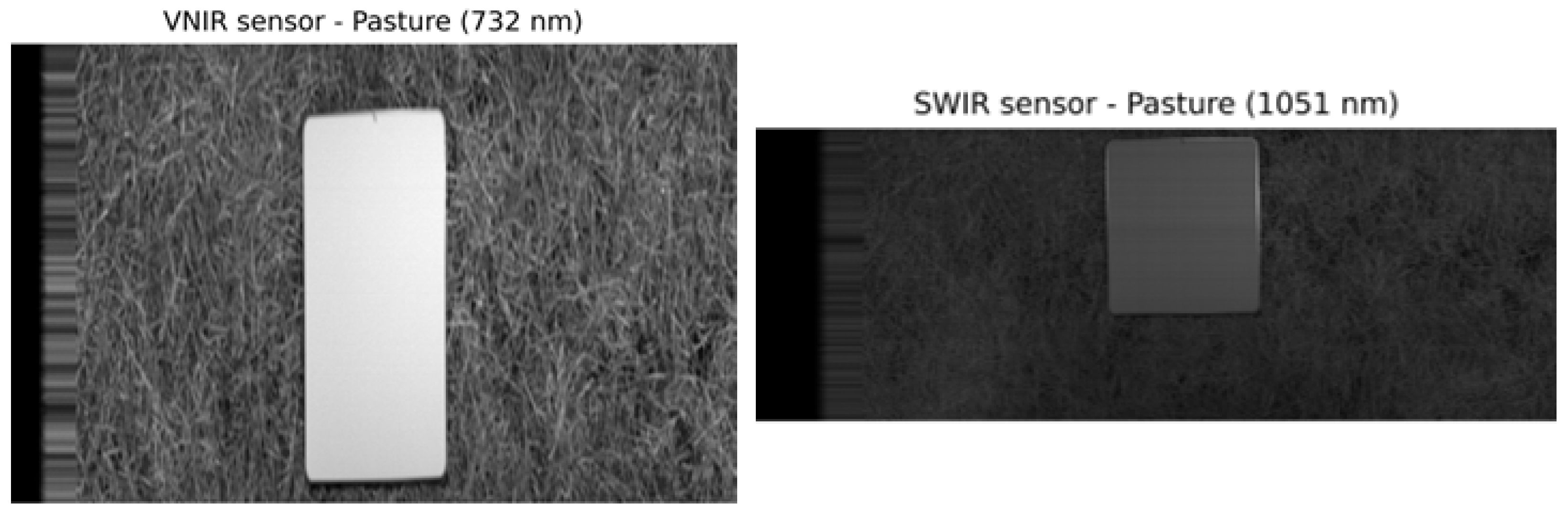
Figure 6 and Figure 7 show the spectral signatures of each fuel type and treatment, before and after each burn, respectively (see Appendix B for examples of the actual imagery for each fuel type). The spectral information is shown per sensor to avoid introducing artefacts into the spectral signatures. The left column of each figure shows the median reflectance across replicates for the Low and High Combustibility treatments. The right columns show the difference in reflectance between the median reflectance of each fuel type (i.e., both treatments) and the median reflectance of the Low and High Combustibility treatments for that fuel type. In the right column, wider differences in reflectance mean that the treatments have higher or lower reflectance than the median spectral for that fuel type in that region of the spectrum. These results highlight both the absolute spectral separation between fuel treatments and the wavelength ranges with the strongest contrasts. For example, in Eucalypt Canopy fuels, the treatments are most different between ~1120–1800 nm (>8%), whereas Eucalypt Litter and Grass Pasture are spectrally very similar in the 400–900 nm range, where there are only small differences (<2%) in reflectance. Implications of these results for satellite instrument design and data product development will be analysed in a separate publication, as will the evaluation of the individual combustion experiments and treatments.
Figure 6.
Pre-fire median spectra and interquartile range (IQR, 25th–75th percentiles) (left column) and deviation of the median spectra of each fuel treatment from the pre-burn median spectra of each fuel type (right column). Top row: Eucalypt Canopy (a,b); middle row: Eucalypt Litter (c,d); bottom row: Grass Pasture (e,f). Solid lines represent the Low Combustibility treatment while dashed lines represent the High Combustibility. For clarity, data within the atmospheric absorption windows have been removed. The spectral range of each sensor is shown at the top of each subplot.
Figure 7.
Post-fire median spectra and interquartile range (IQR, 25th–75th percentiles) (left column) and deviation of the median spectra of each fuel treatment from the post-burn median spectra of each fuel type (right column). Top row: Eucalypt Canopy (a,b); middle row: Eucalypt Litter (c,d); bottom row: Grass Pasture (e,f). Solid lines represent the Low Combustibility treatment while dashed lines represent the High Combustibility. For clarity, data within the atmospheric absorption windows have been removed. The spectral range of each sensor is shown at the top of each subplot.
In Eucalypt Canopy (Figure 6a,b), High Combustibility treatments had higher reflectance across most of the spectrum, most notably from 800–2200 nm, which is consistent with their lower leaf water content and the associated reduction in water absorption. In Eucalypt Litter, the main differences between the Low and High Combustibility spectra were between 1050–1300 nm (Figure 6c,d), with this fuel type displaying similar reflectance in the 1400–2500 nm range. Grass Pasture showed the highest reflectance difference between Low and High Combustibility in the 1400–2100 wavelength range (Figure 6e,f). Overall, reflectance differences between Low and High Combustibility treatments were largest in the Eucalypt Canopy, consistent with the greater FMC contrast between these treatments.
Post-burn spectral data (Figure 7) can be used to infer the degree of fuel consumption by comparing it with the pre-fire spectral signatures. In Eucalypt Canopy (Figure 7a,b), the Low Combustibility treatment showed no change post-burn because these fuels did not ignite. In contrast, the High Combustibility treatment showed reduced reflectance values in the 750–2450 nm range compared to pre-burn, consistent with a partial burn resulting from the fire not reaching the end of the fuel bed (see Table 4).
The spectral response of Eucalypt Litter (Figure 7c,d) and Grass Pasture (Figure 7e,f) in the post-fire scans changed markedly compared to pre-fire as a consequence of the fuel beds being mostly or completely burned. A greater proportion of unburnt material occurred in the Low Combustibility Eucalypt Litter treatment, which increased its median reflectance compared to the High Combustibility treatment, consistent with less complete combustion and a lower cumulative rate of spread in this fuel type (Table 4). For both Grass Pasture fuel treatments, post-fire reflectance was consistently near zero across the spectrum, consistent with surfaces dominated by blackened and charred material, in line with the high cumulative rates of spread and near-complete fuel consumption (Table 4).
3.4. Biochemistry and Calorimetry
Biochemical analyses are shown in Figure 8. Leaf area was similar for High and Low Combustibility treatments of Eucalypt Litter and Grass Pasture. In contrast, Eucalypt Canopy samples from the High Combustibility treatment had a narrower spread of leaf area values than those from the Low Combustibility treatment (Figure 8a). Despite this difference, none of the fuel types showed statistically significant differences in leaf area between treatments (see Table A1).
Figure 8.
Box plots of biochemical characteristics by fuel type and treatment: (a) leaf area, (b) carotenoid content, (c) chlorophyll a, (d) chlorophyll b, (e) cellulose content, and (f) carbon content. Boxes represent the 25th–75th percentiles, horizontal lines the median, whiskers the range, and symbols (◯) individual data points.
Pigment concentrations varied by fuel type (Figure 8b–d). Low Combustibility Eucalypt Canopy samples had notably higher concentrations of carotenoids, chlorophyll a, and chlorophyll b than the corresponding High Combustibility samples, and were approximately one order of magnitude greater than either treatment of both Eucalypt Litter and Grass Pasture fuels. Higher chlorophyll and carotenoid concentrations are consistent with the absorption features observed around 480 nm and 675 nm in the Eucalypt Canopy spectra. The ability to do side-by-side comparisons between treatments and samples highlights the value of the method presented here.
Total cellulose and carbon content (Figure 8e,f) were measured as a percentage of sample wet mass as indicators of structural and non-structural carbohydrates. Carbon content showed significant differences across fuel types and treatments, while cellulose content differed significantly between fuel types but not between treatments. Although cellulose content did not differ between treatments and thus played no role in influencing fire behaviour within a fuel type, the significant differences observed between fuel types, and the known influence of cellulose on reflectance between 1200–2300 nm, support further investigation into how spectral variation across fuel types may relate to cellulose concentration.
Figure 9 shows the calorimetry results for the HHV across fuel types and treatments. No statistically significant differences were detected between treatments for the dead fuel types (Eucalypt Litter and Grass Pasture), although Grass Pasture HHV approached significance between treatments (p ≈ 0.1). Only the Eucalypt Canopy fuel showed a statistically significant difference in HHV between fuel treatments, with High Combustibility samples having higher HHV than the Low Combustibility (i.e., live) samples (p < 0.01).
Figure 9.
Box plots of calorimetry results as high heating value (MJ kg−1) by fuel type and treatment. Boxes represent the 25th–75th percentiles, horizontal lines the median, whiskers the range, and symbols (◯) individual data points.
3.5. GHG and Particulate Emissions
MCE ranged from 0.93 to 0.98 across all burns, indicating combustion that was predominantly flaming in character throughout the experiments. However, flaming and smouldering combustion occurred simultaneously throughout the burns and could not be fully separated spatially or temporally, with active flaming typically occurring at the advancing fire front, while smouldering combustion persisted in the trailing burned fuel bed. Higher MCE values were generally observed during the initial active fire spread phase, while comparatively lower values occurred during the subsequent burnout phase after active fire spread had ceased, suggesting a relatively greater contribution from residual smouldering combustion. The lowest MCE was measured during a High Combustibility Eucalypt Litter burn, which also produced both the highest and lowest MCE values among the Eucalypt Litter burns.
The mixed-combustion period extended from the end of forward fire spread through to the point where CO, CO2, CH4, and PM2.5 concentrations had declined to near-ambient levels. In short-lived burns dominated by flaming, this phase was typically brief. In longer, less intense burns, the mixed phase could persist for an extended period and often included substantial smouldering contributions. It should be noted that in such cases, smouldering combustion may also influence the flaming-dominated interval.
EFs for CH4 and PM2.5 increased with decreasing MCE. Linear regression analyses showed a strong relationship between MCE and EF(CH4) (R2 = 0.95) and a moderate relationship for EF(PM2.5) (R2 = 0.41), with greater scatter in the PM2.5 data (Figure 10).
Figure 10.
Relationship between modified combustion efficiency (MCE) and emissions factors for CH4 (top) and PM2.5 (bottom). Points represent replicate burns, coloured by fuel type (green = Eucalypt Canopy, brown = Eucalypt Litter, yellow = Grass Pasture) and shaped by treatment (square = Low Combustibility, circle = High Combustibility).
The weaker correlation for PM2.5 likely reflects the influence of additional factors that can contribute to variability in particulate emissions, such as combustion temperature. The strength of the correlation between MCE and EF(CH4) indicates the dilution system had little effect on the ratio of concentration enhancements for the measured gaseous species, supporting the reliability of the measurements.
Figure 11 summarises EFs for CO, CO2, CH4, and PM2.5 by fuel type and treatment. The results show generally consistent differences between fuel treatments within each fuel type. EF(CO2) was higher for High Combustibility burns, whereas EF(CO), EF(CH4), and EF(PM2.5)—species typically associated with less efficient combustion—were higher in Low Combustibility treatments. No emissions were measured for the Low Combustibility Eucalypt Canopy treatment since it failed to ignite.
Figure 11.
Emissions factors for (a) CO, (b) CO2, (c) CH4, and (d) PM2.5 by fuel type and treatment. Boxes represent the 25th–75th percentiles, horizontal lines the median, whiskers the range, and symbols (◯) individual data points.
Statistical testing (Table A1) indicated that only the EFs for the treatments of Grass Pasture differed significantly (p < 0.05). For Eucalypt Litter, EFs of the gaseous species were not significantly different (p ≈ 0.3) and EF(PM2.5) was similar (p ≈ 0.2). The similarity in EF(PM2.5) between treatments in this fuel type is consistent with calorimetry results (Figure 9), suggesting that fuel heating value may be a stronger driver of PM emissions than combustibility. Large variability in gaseous EFs was observed in High Combustibility Eucalypt Litter burns, whereas EF(PM2.5) showed relatively low variability in this fuel type and treatment.
Because emissions ratios and emissions factors were derived from synchronised concentration enhancements, uncertainty associated with absolute dilution-ratio stability was considered to be of secondary importance. Gas-phase emissions ratios were therefore assigned an estimated expanded uncertainty of approximately 5%, while gas-phase emissions factors were assigned an uncertainty of 5–10%. For PM2.5, an expanded uncertainty of approximately 30% was adopted for DustTrak DRX-derived emissions factors, primarily reflecting uncertainty associated with aerosol-specific optical response, potential humidity and semi-volatile artefacts, and particle transport losses within the sampling line. The DustTrak was zero-calibrated prior to each experimental run, leak probability within the sampling system was considered negligible, and instrument timing and synchronisation errors were assumed to be minimal.
3.6. Consolidated Results Analysis
PLSR models that used spectral and biophysical information to predict fire behaviour outperformed models that used spectral or biophysical information on their own (Table 5). Models for cumulative rate of spread as time of travel from ignition (i.e., Time to 3.0 metres), flame temperature, and flame height showed the strongest predictive power with Q2 values ranging from 0.72 to 0.836 and RPD from 1.889 to 2.466. One of the top 10 performing models used biophysical data only (Q2 = 0.736, RPD = 1.945), six models used a combination of spectral and biophysical information, and the remaining three models used spectral information only. Models that used only SWIR or SWIR and biophysical information (1.15 > RPD) did not perform as well as models that included spectral information used either the full spectrum or the VNIR region only, suggesting that, under the conditions tested here, SWIR bands contribute predictive capacity as part of the full spectrum models.
Table 5.
Summary statistics for the 10 highest-ranked fire behaviour models (RPD ≥ 1.4, sorted by descending Q2), followed after dashed line by the five best-performing emissions models regardless of RPD threshold (also sorted by descending Q2 (CV)).
Beyond rate of spread, the models accurately predicted Mean flame temperature (°C) (0.826 ≥ Q2 = 0.735, 2.4 ≥ RPD ≥ 1.941) and Max. flame height (mm) (0. 751 ≥ Q2 = 0.742, 2.003 ≥ RPD ≥ 1.968) using both spectral and biophysical information. This indicates that pre-fire fuel bed condition and biochemistry contained information relevant to predicting fuel flammability and fire behaviour. Notably, models that predicted fire behaviour outperformed models that predicted emissions or combustion efficiency under the conditions tested here. The five best-performing models for emissions had much lower Q2 scores (0.641 ≥ Q2 ≥ 0.479) when compared to fire behaviour models, and none was informed by wavelengths in the SWIR region. Additional research is needed to understand the relationship between spectral information in the 400–2500 nm range and gas and particulate emissions from vegetation combustion.
There were three VNIR regions that resulted in high VIP scores in the best-performing models: 500–600 nm, 650–700 nm, and 920–990 nm (Figure 12). The spectral signatures of the three fuel types used here showed distinct characteristics in these three regions (Figure 6), indicating that the PLSR models effectively captured the differences in pigment concentration and fuel dryness. The 650–700 nm region corresponds to the chlorophyll red region absorption feature, where differences between fuel types are most pronounced (Figure 6). The 500–600 nm region is associated with carotenoid and flavonoid pigment absorption, which vary with vegetation senescence and photosynthetic capacity (see Figure 8). Lastly, the 900–990 nm region is strongly influenced by leaf cell structure and water content, both of which differ between fuel types (Figure 6).
Figure 12.
Spectral regions that contribute to higher predictive power in selected PLSR models, shown as Variable Importance in Projection (VIP). Wavelengths where VIP ≥ 1.0 are considered informative. Only models that use spectral information are shown. Target variables shown are those that showed the best performance in Table 5. Dashed line delineates lower performing emission variables. For clarity, wavelengths below 430 nm in the emissions models were excluded from this graph.
In the SWIR region, bands with the highest VIP scores were concentrated in three absorption zones: 1200–1320 nm, 1450–1550 nm, and 1950–2050 nm. These regions provide information on the cell structure, water content and dry matter content of the fuels. These three regions displayed differences between the three fuel types, especially in the two combustibility treatments of Eucalypt Canopy and Grass Pasture fuels (Figure 6a,e). Interestingly, models predicting the time taken for the flame front to reach the 3.0 m mark (the cumulative rate of spread) relied on only VNIR wavelengths, suggesting that VNIR spectral features associated with vegetation condition may contain information relevant to fire spread. In models related to emissions, wavelengths ≤ 430 nm showed the highest VIP scores across all models (VIP > 3); however, these wavelengths were excluded from the analysis because they may have been influenced by instrument noise.
4. Discussion
Despite the complexity of the experimental design, which comprised four integrated research elements, the pilot study successfully achieved measurably different fuel conditions (i.e., combustibility) across the three fuel types: Eucalypt Canopy, Eucalypt Litter, and Grass Pasture. Statistically significant differences in FMC between treatments (Figure 4) confirmed that the combustibility manipulation was effective, providing confidence that observed differences in spectral response, fire behaviour, biochemistry, and emissions were largely attributable to the intended differences in combustibility.
The strong relationship between each fuel treatment’s combustibility and observed fire behaviour (Figure 5) was expected given the known influence of FMC on wildland fire behaviour (i.e., rate of combustion, flame propagation, and flame characteristics), particularly in regard to combustion of dead fuels (Litter and Pasture). The variability seen in the ‘live’ Canopy fuels reflected marginal burning behaviour in the High Combustibility treatment, in which only one of the four replicates successfully spread, while the remaining replicates and those of the Low Combustibility treatment did not spread at all. Although the fire behaviour differed significantly between treatments of the Eucalypt Litter and Grass Pasture fuel types, the absolute differences in the FMC values achieved in the two treatments of these fuels were narrower than planned, limiting the contrast between combustibility levels in these fuels. Despite repeated efforts to increase the FMC of the Low Combustibility treatment of the Eucalypt Litter closer to the limit of combustibility (i.e., the moisture content of extinction is 22–28% ODW for eucalypt litter and 20–24% ODW for grass [7]), all but one replicate of this treatment sustained propagation, albeit at a reduced rate. This may have reduced the contrast between treatments in measurements such as spectral reflectance and emissions, as the Low Combustibility treatments across the dead fuel types contained a mixture of actively propagating flame fronts and more marginal smouldering combustion. Consequently, differences in spectral reflectance and emissions between treatments in these fuels were less distinct than anticipated.
The range of EFs measured agreed with previous experimental burns conducted in the Pyrotron [30]. The strong correlation between CH4 and MCE further indicates that the sampling and analysis methods were reliable for gaseous species. During early burns, dilution applied in the initial flaming phase caused CO, CO2 and particulate concentrations to approach background levels, increasing measurement uncertainty. Future work should include an evaluation of the dilution system to minimise over-dilution and improve measurement accuracy. A longer fuel bed with a mixture of high and low combustible fuels would provide an opportunity to conduct a robust test of dilution processes with the goal of maintaining concentrations in an optimum band. Maintaining a tight range of concentrations is problematic due to rapid increases and decreases in absolute concentrations observed as a burn progresses and transitions between flaming and smouldering phases occur. Flaming combustion consuming large amounts of fuel in a short period of time increases the absolute concentrations of emitted species, requiring rapidly higher levels of dilution. The current dilution processes, while able to protect the instrumentation from high concentrations, were sometimes over-reactive, resulting in inconsistent concentrations (too high or too low) during critical stages of combustion.
The high variability observed in the Eucalypt Litter emission results can be attributed to combustion conditions, reflecting the broad mix of simultaneous combustion modes involving both flaming and smouldering, and the extended duration of the smouldering phase. Minor differences in litter composition (e.g., a higher bark fraction in one sample), FMC and atmospheric relative humidity conditions may also have contributed to this variability. For fuels other than the High Combustibility Eucalypt Litter, the relationship between combustion emissions (gases and particulates) and fuel combustibility (Figure 11) was strong. Over-dilution of concentrations to background values during the flaming phase in some burns may have skewed total fire emissions factors towards the smouldering phase. Further study on the differences between the flaming and mixed flaming/smouldering phase would improve the understanding of such emissions.
Analysis of fuel biochemistry (Figure 8) and energy content (Figure 9) showed little statistically significant difference between treatments in the dead fuels (Eucalypt Litter and Grass Pasture). Slightly greater differences (but still not statistically significant, p = 0.09 for chlorophyll a) were seen in the ‘live’ fuels (i.e., Eucalypt Canopy), presumably because the fuel was still undergoing desiccation, resulting in chemical changes in complex compounds such as chlorophyll and carotenoids.
A critical component of the project was the collection of spectral reflectance data for the chosen fuel types and their treatments. Figure 6 and Figure 7 showed a clear difference in the spectral signatures in the pre- and post-fire scans of the dead fuels (i.e., Eucalypt Litter and Grass Pasture), reflecting successful ignition and fire propagation. Less difference was observed between the pre- and post-fire scans in the ‘live’ fuels (i.e., Eucalypt Canopy), which, if they burned, did so poorly or incompletely, resulting in mixed burned and unburned spectra.
The wide interquartile ranges in the pre-burn spectroscope data led to overlap between treatments of individual fuel types (most apparent in the dead fuels), implying little perceived statistical difference between the treatments. However, this large spread was expected given the interquartile range reflected the full range of samples across all replicates, including the associated spatial variability in illumination, shading and surface orientation of the fuels.
While the analysis of the median spectra undertaken for this article was preliminary, Figure 6 and Figure 7 demonstrate sufficient differentiation in the spectral response between live and dead fuels and, in the case of live fuels, between treatments, to confirm that the methodology can help in resolving fuel combustibility from pre-fire spectral characteristics. While there are obvious differences between the spectra of live and dead fuels, more research is required to conclusively determine whether the spectra of dead fuels can be used to discern differences in moisture content or their biochemical composition, or by the physical and structural characteristics of the fuels. Further analysis is needed to quantitatively investigate spectra retrieved at the level of individual replicates, particularly of dead fuels, and more conclusively identify how the spectral information (i.e., specific wavelengths or bands) could be used for practical measurement of fuel combustibility using remote sensing operationally. Because the low combustibility treatments in the dead fuels still supported sustained fire spread, there is scope to increase the FMC of these treatments further to the moisture content of extinction where combustion is not sustained. Achieving higher FMC levels will require additional work to develop better methods to effectively and consistently increase the absorption of moisture by those fuels.
In this pilot-study, pre-fire spectral reflectance demonstrated substantial predictive power for a range of fire behaviour metrics, including rate of spread, flame height, and flame temperature. In line with the literature [44,52,53], our results suggest that the PLSR models captured the differences in the spectral signatures of fuels in the regions associated with water content, cell structure, and chlorophyll absorption. Variable of Importance in Projection (VIP) results showed that wavelengths that were highly informative for PLSR modes coincided with the regions where the spectral signatures of the three fuel types were the most different (Figure 6 and Figure 12). Full-range spectral data combined with biophysical information resulted in the highest predictive power, indicating that water content and fuel structural properties may be particularly informative for predicting fire behaviour.
Despite good performance on the fire behaviour metrics, none of the emissions models achieved the highest predictive accuracy; moreover, none of the best-performing emissions models used the SWIR wavelengths as predictor variables. These results highlight a gap in our understanding of the relationships between spectral information of vegetation fuels and a fuel’s combustion efficiency and emissions. We also found that several calibration R2 values were high (R2 > 0.9) but achieved only moderate predictive power during the cross-validation (0.9 > Q2 > 0.6), which is a known pattern consistent with overfitting when a limited number of samples are available. Although the use of seven-fold cross-validation and the one-standard-error rule for latent variable selection helped reduce overfitting, the small sample size inherent to this experiment remains a constraint. Despite these issues, our results validated the premise of this experimental set-up and open the possibility for expanded and extended spectral and combustion experiments.
Conducting spectral measurements of fuels pre- and post-burn within the controlled combustion environment of the Pyrotron makes it possible to precisely measure the change in reflectance that occurs following fires of known fireline intensity in fuels of different types with different levels of FMC and combustibility, which would enable a more fundamental assessment of burn severity. Quantification of this relationship will be an important component of future analyses and could enable a more mechanistic assessment of burn severity than current approaches. Current methods relate the difference between burned and unburned pixels where the pre-burn fuel state is often not systematically quantified, and post-burn fuel state cannot practically be measured. Furthermore, the inclusion of GHG and particulate emission measurements in the methodology makes it possible to link the change in spectral response pre- and post-fire to the amount of GHG and particulates emitted from a fire. Improvements to the dilution methodology and increased sample size would provide an opportunity to more deeply explore these links. If a robust relationship were found, this would provide another mechanism to estimate the emissions from both wild and prescribed fires, improving emissions inventories and strengthening climate and air quality forecasts.
The methodology successfully enabled differences in fuel type and combustibility to be quantified via spectral data, though elements of the experimental design, setup and execution could be improved. Adjusting the viewing geometry of the imaging spectrometers to capture more of the fuel bed would expand sampling coverage and improve utility for spatial variability analysis. This may be particularly important for incomplete burns. While substantial effort was put into achieving even halogen lamp illumination across the fuel bed, with generally good results across the spectroscope viewing area, there is capacity to improve lighting uniformity, extend the scanned area, and make the selection of meaningful spectra sampling locations more straightforward.
With the methodology now established and evaluated, future work could extend the collection of spectral data to a broader range of wildland fuels, guided by the hierarchical Australian Bushfire Fuel Classification System [22]. This system provides a robust basis for identifying vegetation classes, fuel types, and combustibility levels important for wildland fire in the Australian landscape. Subject to future resourcing, prioritisation of fuels for investigation could be undertaken in collaboration with Australian rural fire authorities, land management agencies, and other stakeholders, with the longer-term aim of developing a national database linking spectral data with fuel combustibility, fire behaviour, and emissions.
5. Conclusions
This article reported the results of a pilot study evaluating an experimental method to investigate relationships between spectral reflectance (400–2500 nm spectral range) and the combustibility, fire behaviour, and emissions of wildland fuels. The study assessed the feasibility of manipulating the combustibility of common Australian wildland fuels and of directly comparing four complementary measures of fuel characterisation: fuel biochemistry, fire behaviour, fire emissions, and spectral reflectance. This was achieved using a replicated set of free-spreading fire experiments conducted in a large combustion wind tunnel with an air flow of 1.0 m s−1 across three fuel types (live eucalypt canopy leaves, dead eucalypt leaf litter and a dead pasture grass) and two treatments representing the extremes of combustibility (low and high).
The pilot study successfully demonstrated the feasibility and potential utility of the experimental method. Although the preliminary analysis did not reveal strong spectral differentiation between combustibility levels for the dead fuels based on median spectra alone, predictive modelling demonstrated encouraging relationships between pre-fire spectral information and several fire behaviour and emissions metrics. A detailed assessment across a wider range of fuel moisture levels and dead fuels would be valuable to establish the limits of detectability before extending the methodology to additional fuel types and combustibility conditions. Further research is also needed to evaluate the consistency of the relationships observed in this pilot study and to quantify the extent to which fuel condition, fire behaviour, biochemistry and emissions can be inferred from the spectral characteristics of pre- and post-burn fuels.
If applied more broadly across vegetation classes and fuel types, this methodology could contribute to the development of a comprehensive database linking spectral reflectance with fuel combustibility, fire behaviour, and emissions. Such a database could support improved interpretation of historical and future remote sensing datasets, guide new satellite product development, and inform requirements definition for next-generation fire management missions. It could also support broader assessments of vegetation state and fuel condition and enable future research into applications such as burnt area and burn severity mapping, GHG emission estimation, and carbon accounting.
Reliable and timely assessment of fuel condition across landscapes, and the subsequent expected fire behaviour should a fire occur, has the potential to provide fire managers with critical information for both wildfire preparedness and the safe and effective use of prescribed burning for fuel hazard reduction. Integrating such data into fire danger prediction systems could help strengthen the capacity to predict hazardous conditions and plan effective mitigation.
Author Contributions
Conceptualization, A.L.S., N.Y., C.B., A.A. and L.L.; methodology, A.L.S., N.Y., C.T.R., C.B., F.R., A.A. and L.L.; formal analysis, A.L.S., N.Y., C.T.R., F.R., E.H., M.P.P., M.A.A. and M.T.; investigation, A.L.S., E.H., M.P.P., M.A.A., M.T. and M.K.; data curation, N.Y. and M.P.P.; writing—original draft preparation, A.L.S., N.Y., C.T.R. and E.H.; writing—review and editing, A.L.S., C.B., F.R., A.A., M.P.P., M.A.A., M.T., M.K., L.L. and M.Y.; visualization, N.Y. and M.A.A.; project administration, A.L.S., C.B. and A.A.; funding acquisition, C.B. and M.Y. All authors have read and agreed to the published version of the manuscript.
Funding
This research was collectively funded by CSIRO, Geoscience Australia and the Australian National University through the Peter Brabazon Brooke Bushfire Research Fund and the Bushfire Research Centre of Excellence. Marek Tuhý’s contributions to this work were made possible by the Czech Science Foundation (Project No. 23-06344O).
Data Availability Statement
The raw data supporting the conclusions of this article will be made available by the authors on request.
Acknowledgments
The authors acknowledge the expertise of the CSIRO Global Atmospheric Sampling Laboratory (GASLAB), in particular Darren Spencer for instrumentation troubleshooting, sampling support, and planning, and the Aerosols and Reactive Gases (ARG) team in CSIRO Environment, especially James Harnwell and Jason Ward, for their contributions to the design and implementation of the sampling manifold and inlet. We thank Dale Hughes for his work in designing, developing, operating, and maintaining the ANU Forest Spectroscope. We are also grateful to Craig Ingram and Joshua Pease for their assistance in designing and characterising lighting conditions for these experiments, and for supporting the design of the mounting system for the ANU Forest Spectroscope. We also thank Kimberley Clayfield, Libby Pinkard, Raphaele Blanchi and Nick Carter of CSIRO for their support in initiating this project. We acknowledge the laboratory work conducted by Mbam Itumo. Finally, we thank Joshua Pease, Nick Carter, and Amy Parker for their constructive comments on earlier versions of this article. We also thank the four anonymous journal referees whose comments helped greatly to improve the article.
Conflicts of Interest
The authors declare no conflicts of interest. The funders had no role in the design of the study; in the collection, analyses, or interpretation of data; in the writing of the manuscript; or in the decision to publish the results.
Appendix A. Statistical Analysis Results
Table A1.
Summary of statistical analyses of experimental results comparing fuel treatments for each measurement type.
Appendix B. Sample Pre-Fire Spectral Imagery for Each Fuel Type
Figure A1.
Single-band pre-fire imagery for replicate 4 of Eucalypt Canopy High Combustibility experiment.
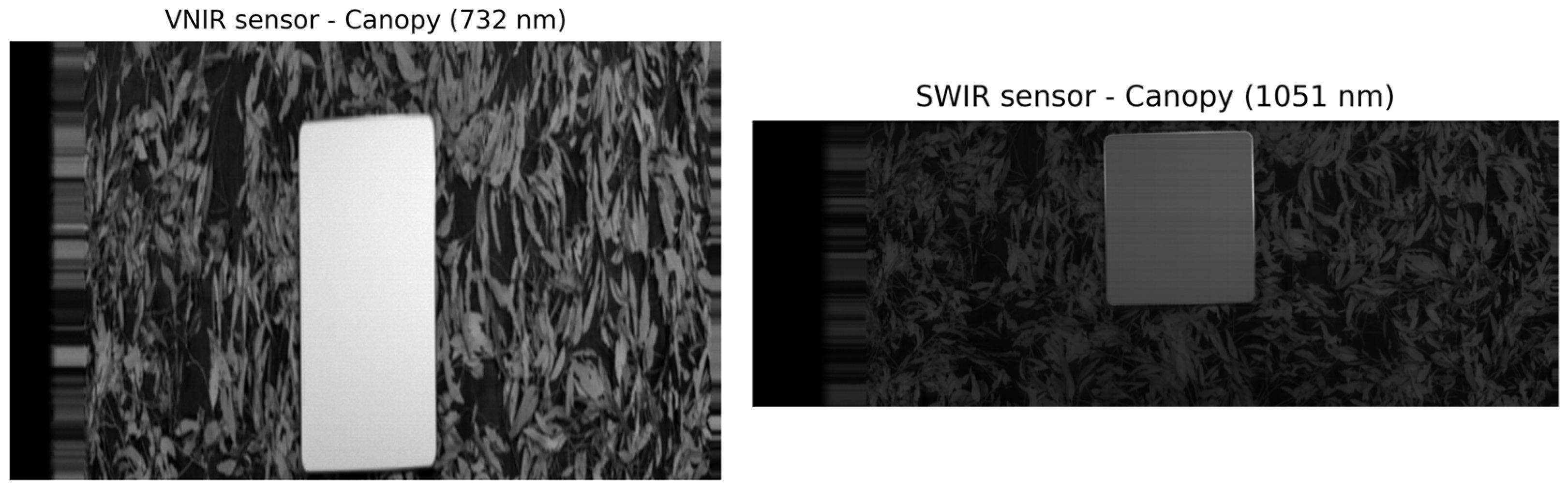
Figure A2.
Single-band pre-fire imagery for replicate 4 of Eucalypt Litter High Combustibility experiment.
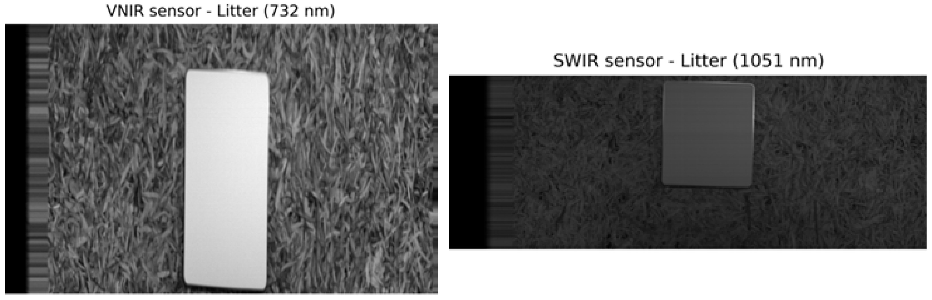
Figure A3.
Single-band pre-fire imagery for replicate 3 of Grass Pasture High Combustibility experiment.
References
- UNEP. Spreading Like Wildfire—The Rising Threat of Extraordinary Landscape Fires: A UNEP Rapid Response Assessment; Sullivan, A.L., Baker, E., Kurvits, T., Eds.; United Nations Environment Programme: Nairobi, Kenya, 2022; 128p. [Google Scholar]
- Cunningham, C.X.; Williamson, G.J.; Bowman, D.M.J.S. Increasing frequency and intensity of the most extreme wildfires on Earth. Nat. Ecol. Evol. 2024, 8, 1420–1425. [Google Scholar] [CrossRef] [Scilit] [PubMed]
- Canadell, J.G.; Meyer, C.P.; Cook, G.D.; Dowdy, A.; Briggs, P.R.; Knauer, J.; Pepler, A.; Haverd, V. Multi-decadal increase of forest burned area in Australia is linked to climate change. Nat. Commun. 2021, 12, 6921. [Google Scholar] [CrossRef] [Scilit] [PubMed]
- Jones, M.W.; Veraverbeke, S.; Andela, N.; Doerr, S.H.; Kolden, C.; Mataveli, G.; Pettinari, M.L.; Le Quéré, C.; Rosan, T.M.; van der Werf, G.R.; et al. Global rise in forest fire emissions linked to climate change in the extratropics. Science 2024, 386, eadl5889. [Google Scholar] [CrossRef] [Scilit] [PubMed]
- Maclean, K.; Hankins, D.L.; Christianson, A.C.; Oliveras, I.; Bilbao, B.A.; Costello, O.; Langer, E.R.; Robinson, C.J. Revitalising Indigenous cultural fire practice: Benefits and partnerships. Trends Ecol. Evol. 2023, 38, 899–902. [Google Scholar] [CrossRef] [Scilit] [PubMed]
- Hiers, J.K.; O’Brien, J.J.; Varner, J.M.; Butler, B.W.; Dickinson, M.; Furman, J.; Gallagher, M.; Godwin, D.; Goodrick, S.L.; Hood, S.M.; et al. Prescribed fire science: The case for a refined research agenda. Fire Ecol. 2020, 16, 11. [Google Scholar] [CrossRef] [Scilit]
- Sullivan, A.L.; McCaw, W.L.; Cruz, M.G.; Matthews, S.; Ellis, P.F. Fuel, fire weather and fire behaviour in Australian ecosystems. In Flammable Australia: Fire Regimes, Biodiversity and Ecosystems in a Changing World; Bradstock, R.A., Gill, A.M., Williams, R.D., Eds.; CSIRO Publishing: Collingwood, Australia, 2012; Chapter 3; pp. 51–77. [Google Scholar]
- Li, F.; Zhang, X.; Cochrane, M.; Kondragunta, S.; An, S. Fire spread, intensity, and emissions observations by multiple satellites: The Southern California wildfires of January 2025. AGU Adv. 2026, 7, e2025AV002064. [Google Scholar] [CrossRef] [Scilit]
- Zhao, J.; Zheng, B.; Ciais, P.; Chen, Y.; Gasser, T.; Canadell, J.G.; Zhang, L.; Zhang, Q. Global warming amplifies wildfire health burden and reshapes inequality. Nature 2025, 647, 928–934. [Google Scholar] [CrossRef] [Scilit] [PubMed]
- Cheney, N.P. Predicting fire behaviour with fire danger tables. Austral. For. 1968, 32, 71–79. [Google Scholar] [CrossRef] [Scilit]
- Chandler, C.; Cheney, P.; Thomas, P.; Trabaud, L.; Williams, D. Fire in Forestry 1: Forest Fire Behaviour and Effects; John Wiley & Sons: New York, NY, USA, 1983; 450p. [Google Scholar]
- Sullivan, A.L. Wildland surface fire spread modelling, 1990–2007. 2: Empirical and quasi-empirical models. Int. J. Wildland Fire 2009, 18, 369–386. [Google Scholar] [CrossRef] [Scilit]
- Plucinski, M.P. Contain and control: Wildfire suppression effectiveness at incidents and across landscapes. Curr. For. Rep. 2019, 5, 20–40. [Google Scholar] [CrossRef] [Scilit]
- IPCC. 2019 Refinement to the 2006 IPCC Guidelines for National Greenhouse Gas Inventories: Volume 4: Agriculture, Forestry and Other Land Use; Buendia, E.C., Tanabe, K., Kranjc, A., Baasansuren, J., Fukuda, M., Ngarize, S., Osako, A., Pyrozhenko, Y., Shermanau, P., Federici, S., Eds.; IGES: Kanagawa, Japan, 2019; Chapter 2. [Google Scholar]
- Surawski, N.C.; Sullivan, A.L.; Roxburgh, S.H.; Meyer, C.P.; Polglase, P.J. Incorrect interpretation of carbon mass balance biases global vegetation fire emission estimates. Nat. Commun. 2016, 7, 11536. [Google Scholar] [CrossRef] [Scilit] [PubMed]
- Cruz, M.G. A comment on the use of visually assessed fuel hazard ratings and scores for Australian fire management and research. Int. J. Wildland Fire 2024, 33, WF23164. [Google Scholar] [CrossRef] [Scilit]
- Dalezios, N.R.; Kalabokidis, K.; Koutsias, N.; Vasilakos, C. Wildfires and remote sensing: An overview. In Remote Sensing of Hydrometeorological Hazards; Petropoulos, G.P., Islam, T., Eds.; CRC Press: Boca Raton, FL, USA, 2017; pp. 211–236. [Google Scholar] [CrossRef] [Scilit]
- Gale, M.G.; Cary, G.J.; Van Dijk, A.I.J.M.; Yebra, M. Forest fire fuel through the lens of remote sensing: Review of approaches, challenges and future directions in the remote sensing of biotic determinants of fire behaviour. Remote Sens. Environ. 2021, 255, 112282. [Google Scholar] [CrossRef] [Scilit]
- Falkowski, M.; Shuman, J.; Boland, J.; Kauffman, T.; Lefer, B.; Martin, M.M.; Riris, H. The NASA FireSense Project: Responding to Stakeholder Needs Across the Fire Life Cycle. In IGARSS 2024—2024 IEEE International Geoscience and Remote Sensing Symposium; IEEE: New York, NY, USA, 2024; pp. 2356–2359. [Google Scholar] [CrossRef] [Scilit]
- Abdollahi, A.; Yebra, M. Challenges and opportunities in remote sensing-based fuel load estimation for wildfire behavior and management: A comprehensive review. Remote Sens. 2025, 17, 415. [Google Scholar] [CrossRef] [Scilit]
- Younes, N.; Yebra, M.; Mathew, J.; Sharp, R. OzFuel: A space-based vegetation fuel flammability monitoring system. In Proceedings of the SPIE 12729 Remote Sensing: Sensors, Systems, and Next-Generation Satellites XXVII; SPIE: Bellingham, WA, USA, 2023; p. 127291B. [Google Scholar] [CrossRef] [Scilit]
- Cruz, M.G.; Gould, J.S.; Hollis, J.J.; McCaw, W.L. A hierarchical classification of wildland fire fuels for Australian vegetation types. Fire 2018, 1, 13. [Google Scholar] [CrossRef] [Scilit]
- Anderson, H.E. Forest fuel ignitability. Fire Technol. 1970, 6, 312–319. [Google Scholar] [CrossRef] [Scilit]
- Matthews, S. Dead fuel moisture research: 1991–2012. Int. J. Wildland Fire 2014, 23, 78–92. [Google Scholar] [CrossRef] [Scilit]
- Wilson, R.A., Jr. Observations of extinction and marginal burning states in free burning porous fuel beds. Combust. Sci. Technol. 1985, 44, 179–193. [Google Scholar] [CrossRef] [Scilit]
- Joshi, R.C.; Cruz, M.G.; Donohue, R.J. Nationally consistent mapping of wildland fuel types across Australia using satellite-derived vegetation structural data. Int. J. Wildland Fire 2025, 34, WF24224. [Google Scholar] [CrossRef] [Scilit]
- Mulvaney, J.J.; Sullivan, A.L.; Cary, G.J.; Bishop, G.R. Repeatability of free-burning fire experiments using heterogeneous forest fuel beds in a combustion wind tunnel. Int. J. Wildland Fire 2016, 25, 445–455. [Google Scholar] [CrossRef] [Scilit]
- Sullivan, A.L.; Knight, I.K.; Hurley, R.; Webber, C. A contractionless, low-turbulence wind tunnel for the study of free-burning fires. Exp. Therm. Fluid Sci. 2013, 44, 264–274. [Google Scholar] [CrossRef] [Scilit]
- Hughes, D.; Younes, N.; Hay, E. ANU Forest Spectroscope Manual, Version 2.0; Technical report; ANU Fenner School, The Australian National University: Canberra, Australia, 2025. [Google Scholar] [CrossRef]
- Guérette, É.-A.; Paton-Walsh, C.; Desservettaz, M.; Reisen, F.; Surawski, N.C.; Meyer, C.P.; Roulston, C.T.; Sullivan, A.; Weston, C.J.; Volkova, L. Simplifying emissions modelling from wildland fires: Laboratory-scale emission factors are independent of fine woody debris fuel load. Int. J. Wildland Fire 2025, 34, WF24117. [Google Scholar] [CrossRef] [Scilit]
- Matthews, S. Effect of drying temperature on fuel moisture content measurements. Int. J. Wildland Fire 2010, 19, 800–802. [Google Scholar] [CrossRef] [Scilit]
- Bruegge, C.J.; Stiegman, A.E.; Rainen, R.A.; Springsteen, A.W. Use of Spectralon as a diffuse reflectance standard for in-flight calibration of earth-orbiting sensors. Opt. Eng. 1993, 32, 805–-814. [Google Scholar] [CrossRef] [Scilit]
- Cain, S.; Younes, N. Cellulose extraction and quantification from eucalyptus leaves in the laboratory, V.1. Protoc. Exch. 2024. [Google Scholar] [CrossRef] [Scilit] [PubMed]
- Younes, N.; Cain, S. Analysis of chlorophyll and carotenoid compounds in eucalyptus leaves, V.1. Protoc. Exch. 2023. [Google Scholar] [CrossRef] [Scilit] [PubMed]
- Younes, N.; Cain, S. Carbon and nitrogen nutrient analysis of eucalyptus leaves, V.1. Protoc. Exch. 2023. [Google Scholar] [CrossRef] [Scilit] [PubMed]
- Ward, D.E.; Radke, L.F. Emission measurements from vegetation fires: A comparative evaluation of methods and results. In Fire in the Environment: The Ecological, Atmospheric and Climatic Importance of Vegetation Fires; Crutzen, P.J., Goldhammer, J.G., Eds.; John Wiley & Sons: Chichester, UK, 1993; Chapter 4; pp. 53–76. [Google Scholar]
- Meyer, C.P.; Cook, G.D.; Reisen, F.; Smith, T.E.L.; Tattaris, M.; Russell-Smith, J.; Maier, S.W.; Yates, C.P.; Wooster, M.J. Direct measurements of the seasonality of emission factors from savanna fires in northern Australia. J. Geophys. Res.-Atmos. 2012, 117, D20305. [Google Scholar] [CrossRef] [Scilit]
- Andreae, M.O.; Merlet, P. Emission of trace gases and aerosols from biomass burning. Glob. Biogeochem. Cycles 2001, 15, 955–966. [Google Scholar] [CrossRef] [Scilit]
- Meyer, C.P.M.; Cook, G.D. Biomass combustion and emission processes in the northern Australian savannas. In Carbon Accounting and Savanna Fire Management; Murphy, B.P., Edwards, A.C., Meyer, C.P.M., Russell-Smith, J., Eds.; CSIRO Publishing: Collingwood, Australia, 2015; pp. 185–217. [Google Scholar]
- Surawski, N.C.; Sullivan, A.L.; Meyer, C.P.; Roxburgh, S.H.; Polglase, P.J. Greenhouse gas emissions from laboratory-scale fires in wildland fuels depend on fire spread mode and phase of combustion. Atmos. Chem. Phys. 2015, 15, 5259–5273. [Google Scholar] [CrossRef] [Scilit]
- Perera, I.E.; Litton, C.D. Quantification of optical and physical properties of combustion-generated carbonaceous aerosols (<PM2.5) using analytical and microscopic techniques. Fire Technol. 2013, 51, 247–269. [Google Scholar] [CrossRef] [Scilit] [PubMed]
- Kothari, S.; Beauchamp-Rioux, R.; Blanchard, F.; Crofts, A.L.; Girard, A.; Guilbeault-Mayers, X.; Hacker, P.W.; Pardo, J.; Schweiger, A.K.; Demers-Thibeault, S.; et al. Predicting leaf traits across functional groups using reflectance spectroscopy. New Phytol. 2023, 238, 549–566. [Google Scholar] [CrossRef] [Scilit] [PubMed]
- Ji, F.; Li, F.; Hao, D.; Shiklomanov, A.N.; Yang, X.; Townsend, P.A.; Dashti, H.; Nakaji, T.; Kovach, K.R.; Liu, H.; et al. Unveiling the transferability of PLSR models for leaf trait estimation: Lessons from a comprehensive analysis with a novel global dataset. New Phytol. 2024, 243, 111–131. [Google Scholar] [CrossRef] [Scilit] [PubMed]
- Serbin, S.P.; Singh, A.; McNeil, B.E.; Kingdon, C.C.; Townsend, P.A. Spectroscopic determination of leaf morphological and biochemical traits for northern temperate and boreal tree species. Ecol. Appl. 2014, 24, 1651–1669. [Google Scholar] [CrossRef] [Scilit] [PubMed]
- Hastie, T.; Tibshirani, R.; Friedman, J. The Elements of Statistical Learning: Data Mining, Inference, and Prediction, 2nd ed.; Springer Series in Statistics; Springer: New York, NY, USA, 2009. [Google Scholar] [CrossRef] [Scilit]
- Chang, C.-W.; Laird, D.A.; Mausbach, M.J.; Hurburgh, C.R. Near-infrared reflectance spectroscopy–principal components regression analyses of soil properties. Soil Sci. Soc. Am. J. 2001, 65, 480–490. [Google Scholar] [CrossRef] [Scilit]
- Hunter, J.D. Matplotlib: A 2D Graphics Environment. Comput. Sci. Eng. 2007, 9, 90–95. [Google Scholar] [CrossRef] [Scilit]
- Pedregosa, F.; Varoquaux, G.; Gramfort, A.; Michel, V.; Thirion, B.; Grisel, O.; Blondel, M.; Prettenhofer, P.; Weiss, R.; Dubourg, V.; et al. Scikit-Learn: Machine Learning in Python. J. Mach. Learn. Res. 2011, 12, 2825–2830. [Google Scholar]
- Virtanen, P.; Gommers, R.; Oliphant, T.E.; Haberland, M.; Reddy, T.; Cournapeau, D.; Burovski, E.; Peterson, P.; Weckesser, W.; Bright, J.; et al. SciPy 1.0: Fundamental algorithms for scientific computing in Python. Nat. Methods 2020, 17, 261–272. [Google Scholar] [CrossRef] [Scilit] [PubMed]
- McKinney, W. Data structures for statistical computing in Python. In Proceedings of the 9th Python in Science Conference (SCIPY 2010), Austin, TX, USA, 28 June–3 July 2010. [Google Scholar] [CrossRef] [Scilit]
- Gould, J.S.; Sullivan, A.L. Two methods for calculating wildland fire rate of forward spread. Int. J. Wildland Fire 2020, 29, 272–281. [Google Scholar] [CrossRef] [Scilit]
- DuBois, S.; Desai, A.R.; Singh, A.; Serbin, S.P.; Goulden, M.L.; Baldocchi, D.D.; Ma, S.; Oechel, W.C.; Wharton, S.; Kruger, E.L.; et al. Using imaging spectroscopy to detect variation in terrestrial ecosystem productivity across a water-stressed landscape. Ecol. Appl. 2018, 28, 1313–1324. [Google Scholar] [CrossRef] [Scilit] [PubMed]
- Meacham-Hensold, K.; Montes, C.M.; Wu, J.; Guan, K.; Fu, P.; Ainsworth, E.A.; Pederson, T.; Moore, C.E.; Brown, K.L.; Raines, C.; et al. High-throughput field phenotyping using hyperspectral reflectance and partial least squares regression (PLSR) reveals genetic modifications to photosynthetic capacity. Remote Sens. Environ. 2019, 231, 111176. [Google Scholar] [CrossRef] [Scilit] [PubMed]
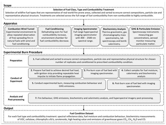
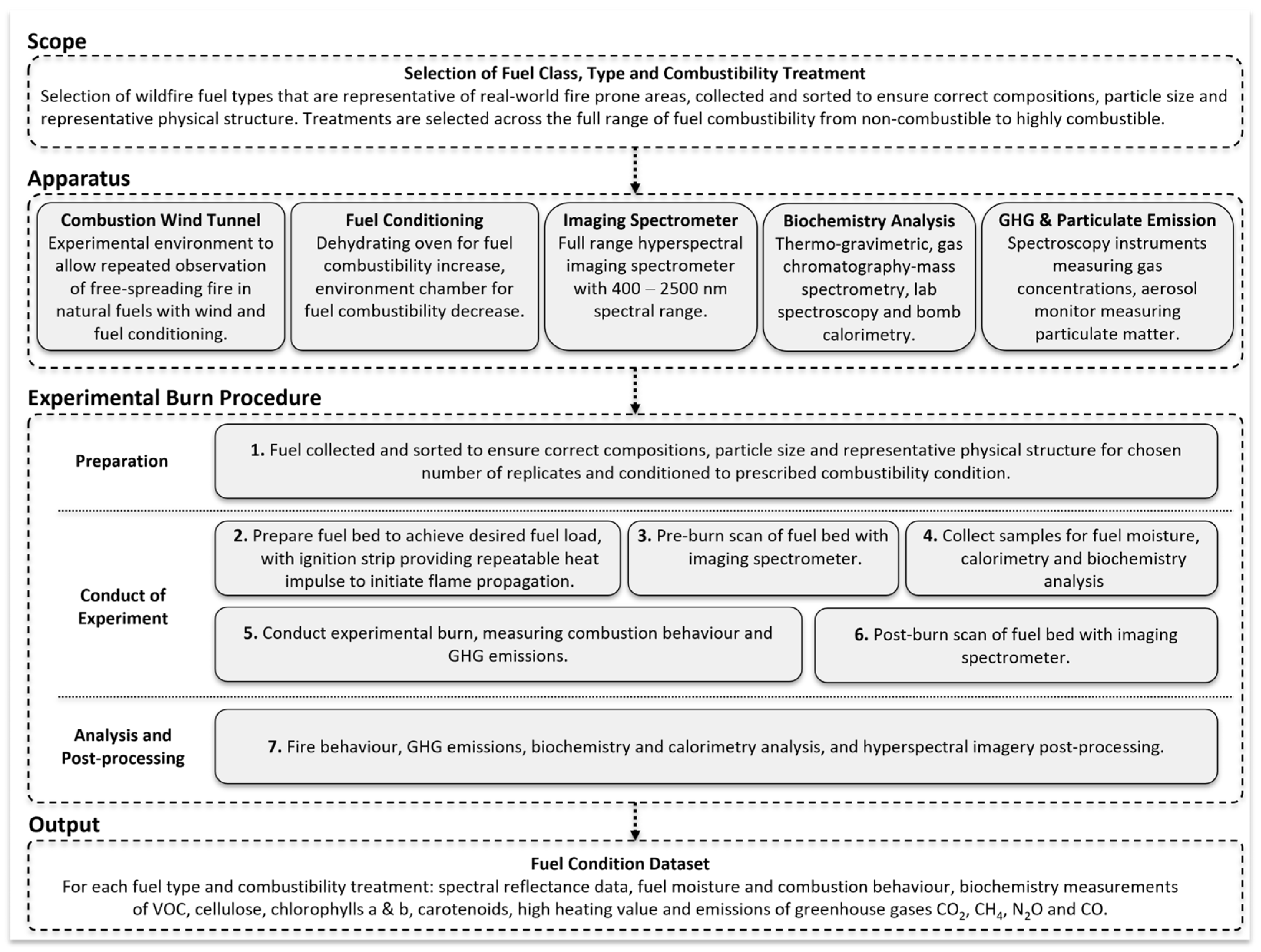
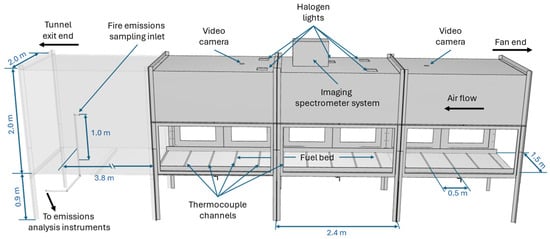
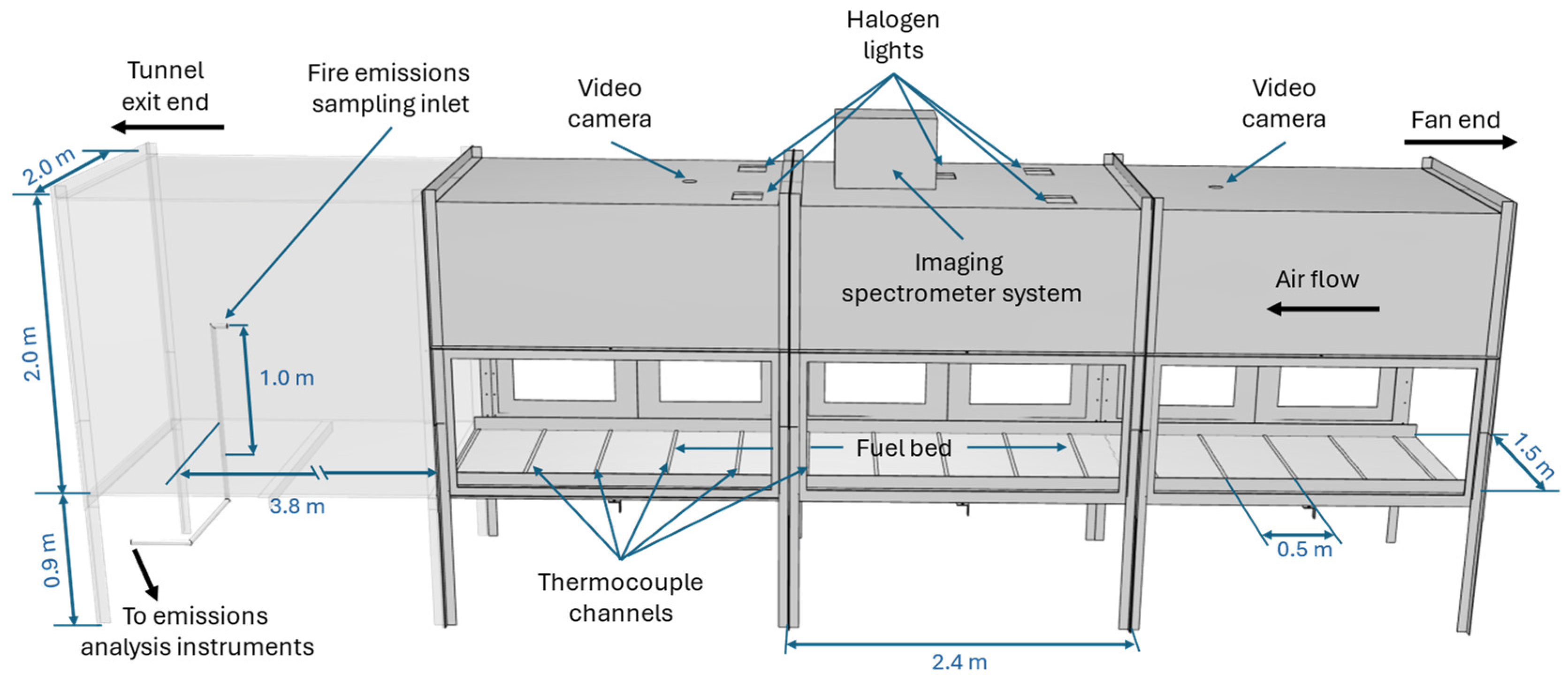
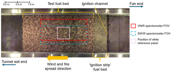
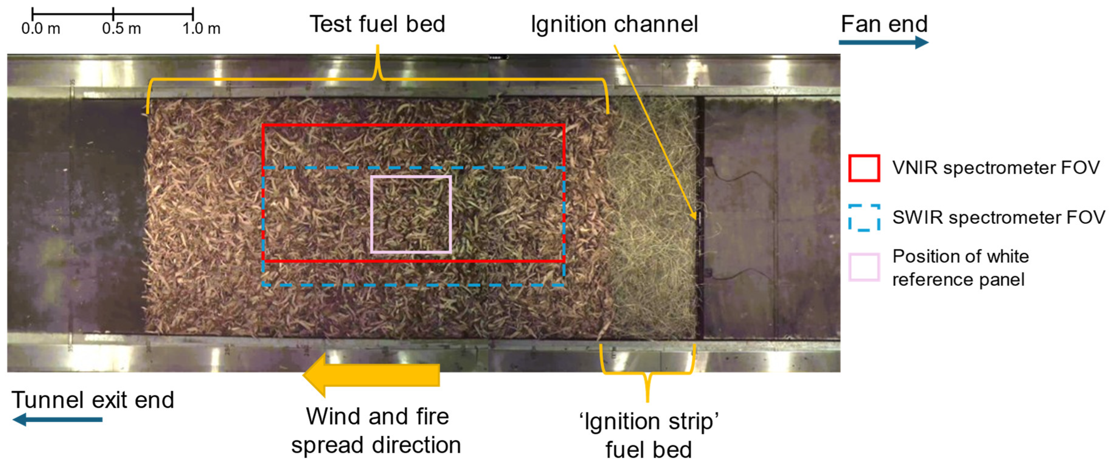
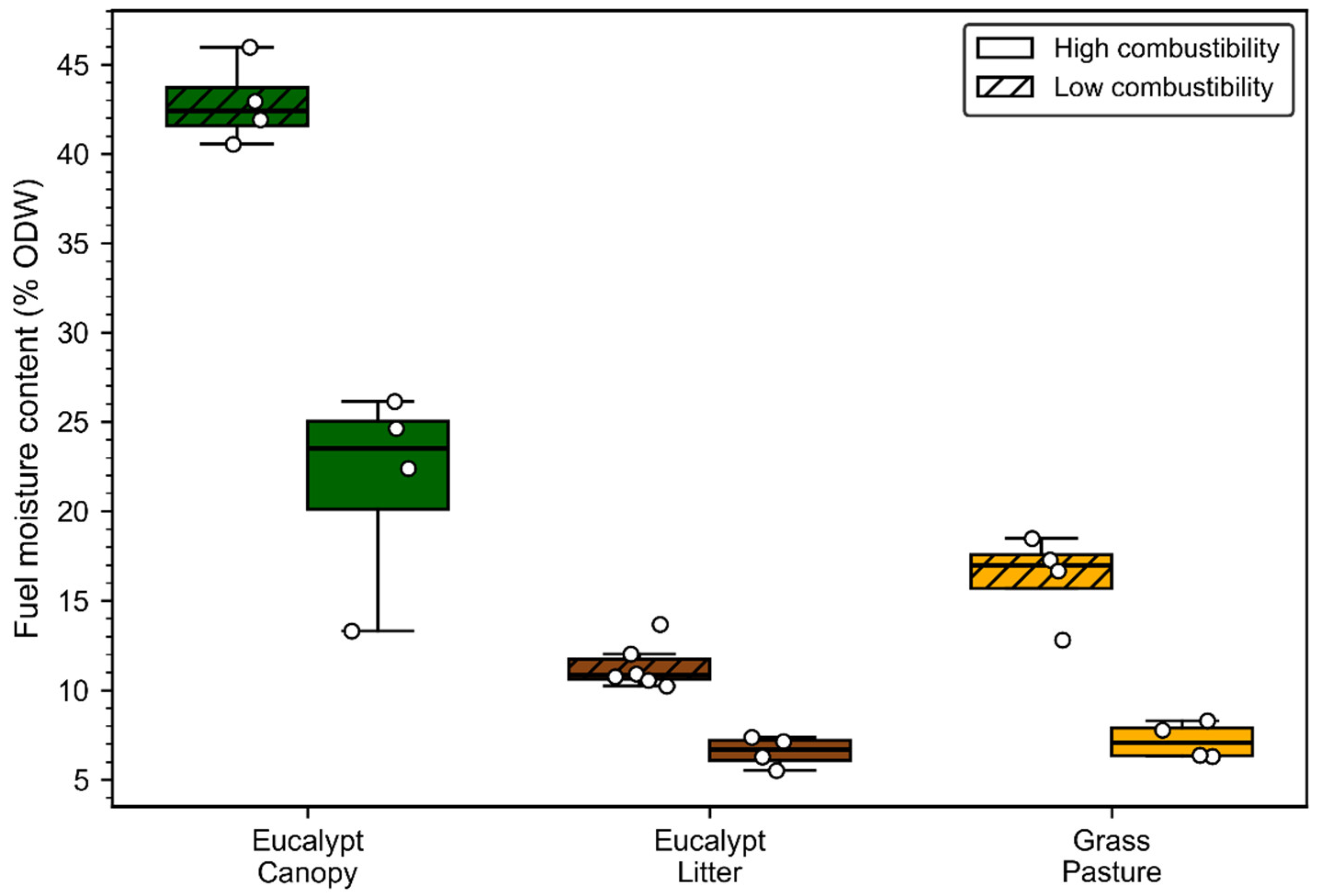
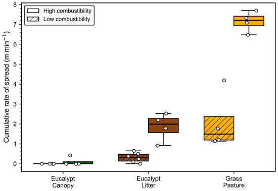
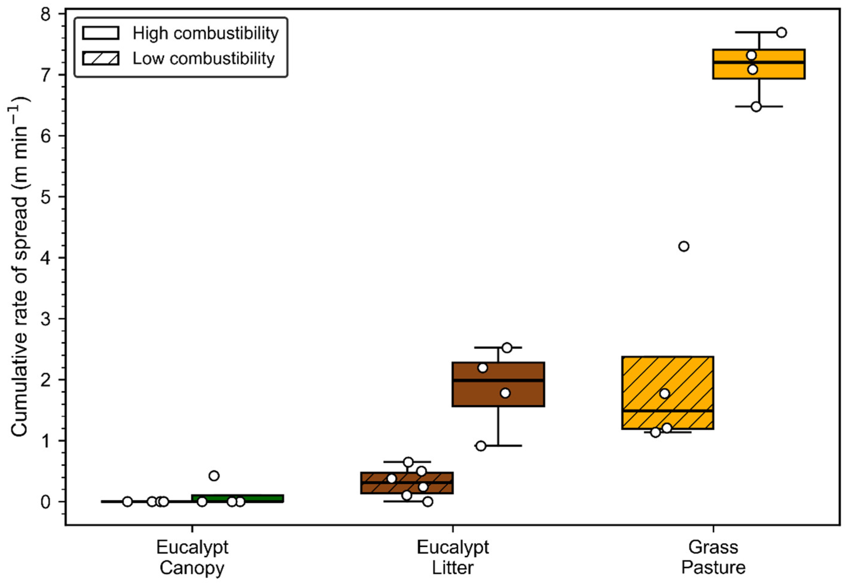
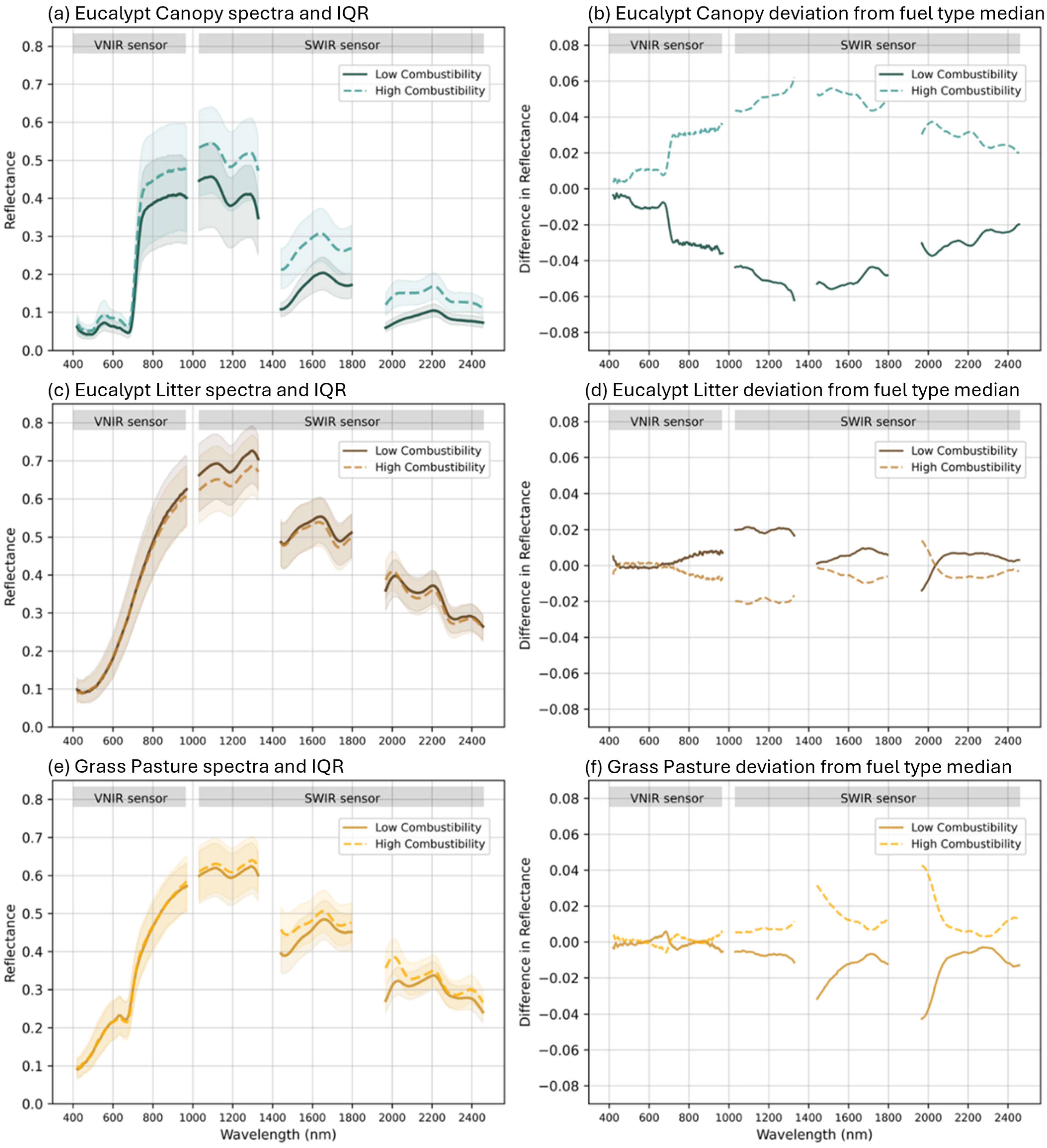
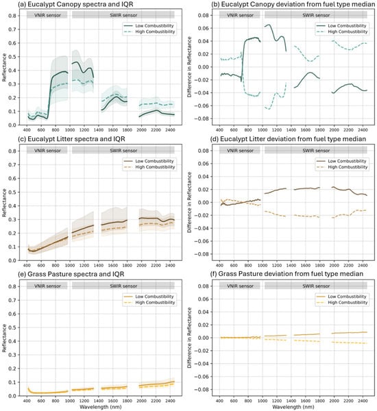
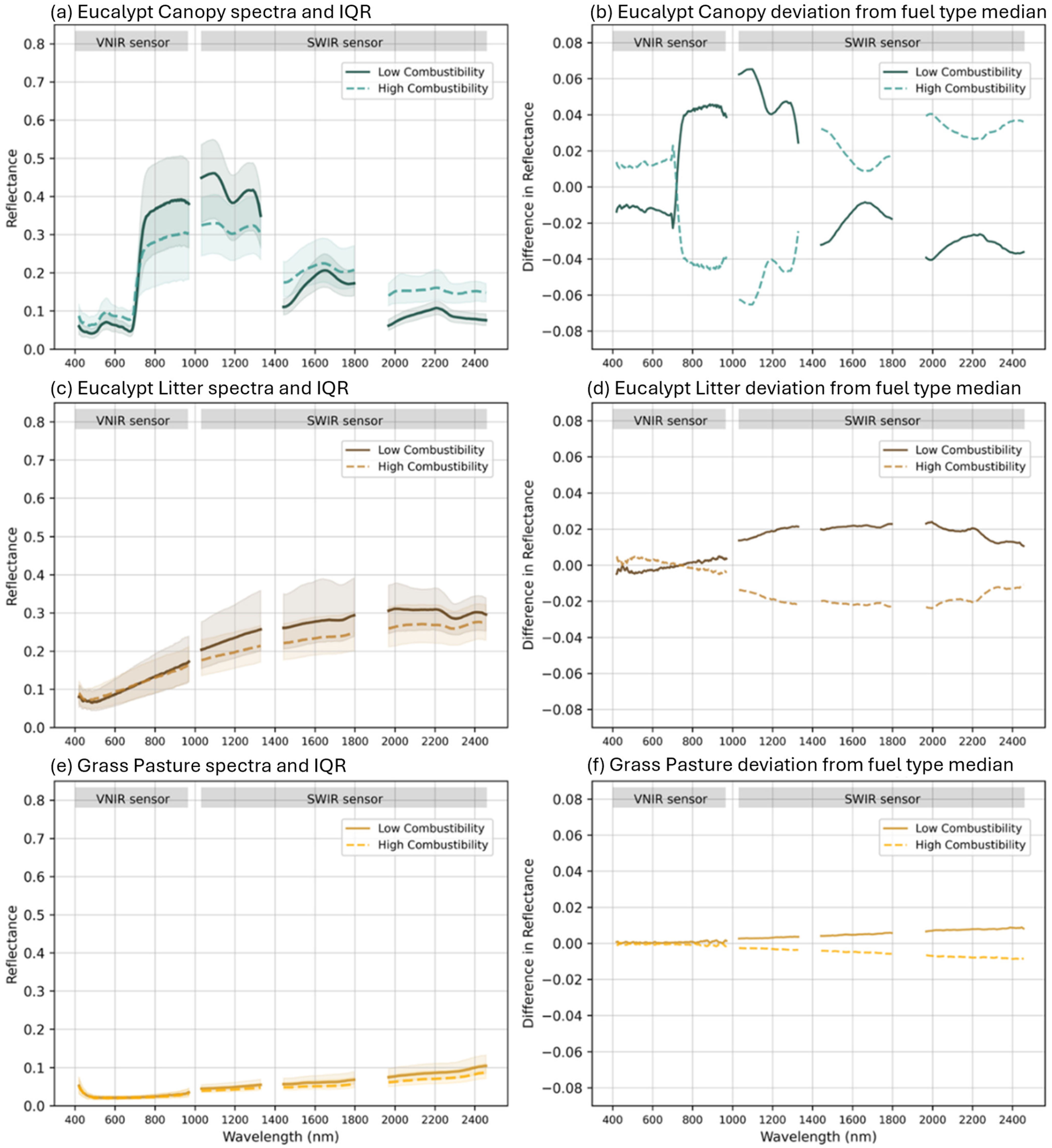
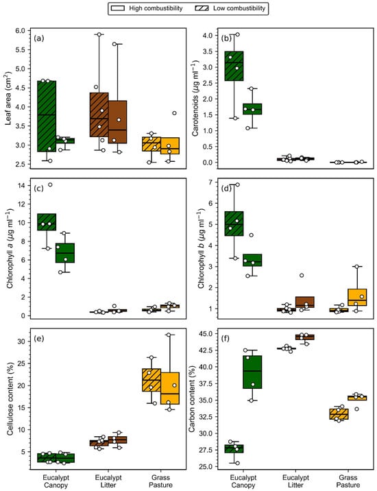
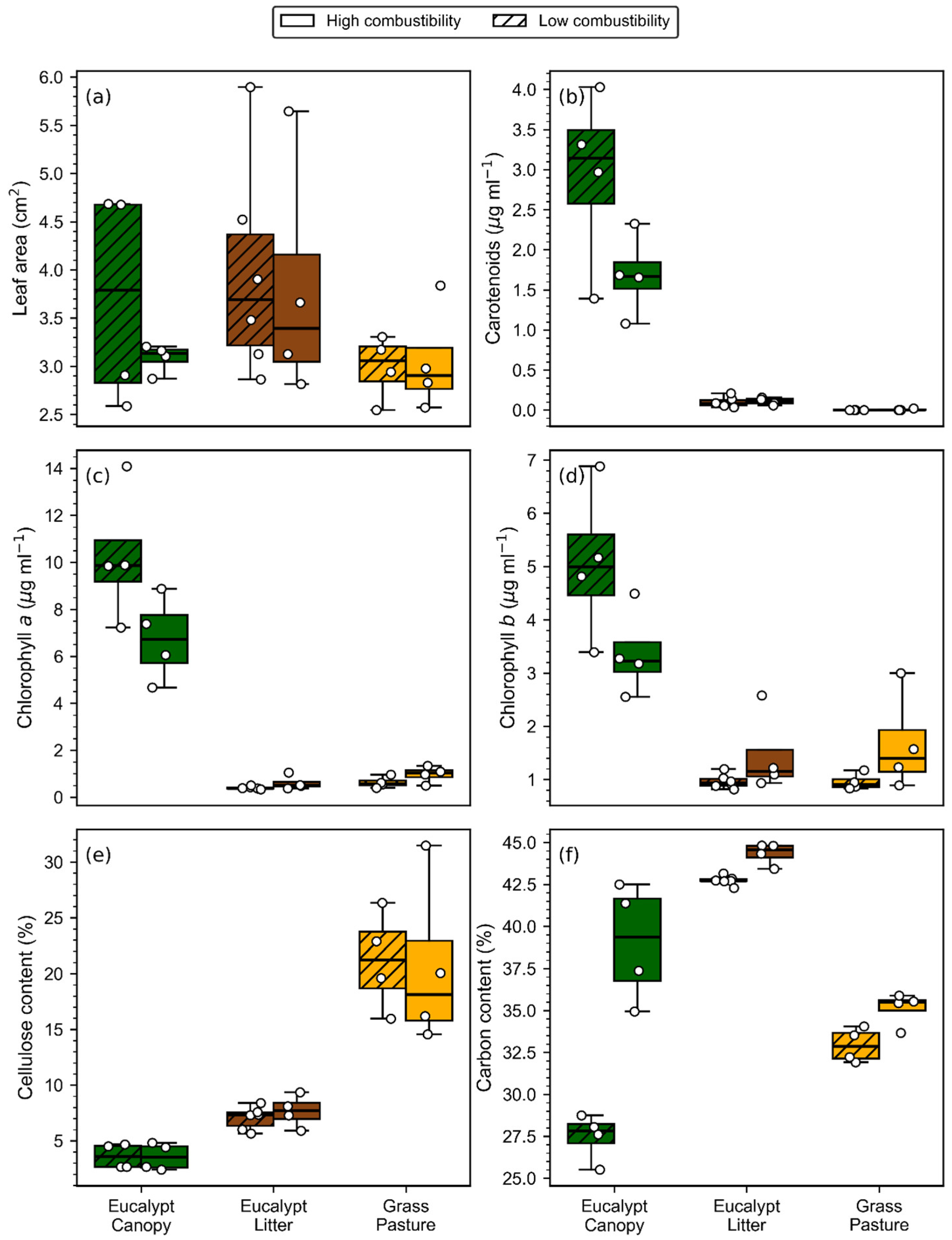
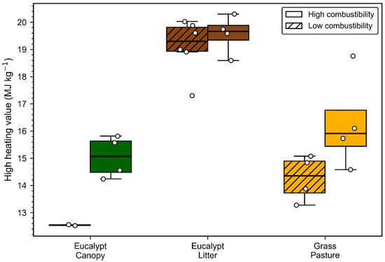
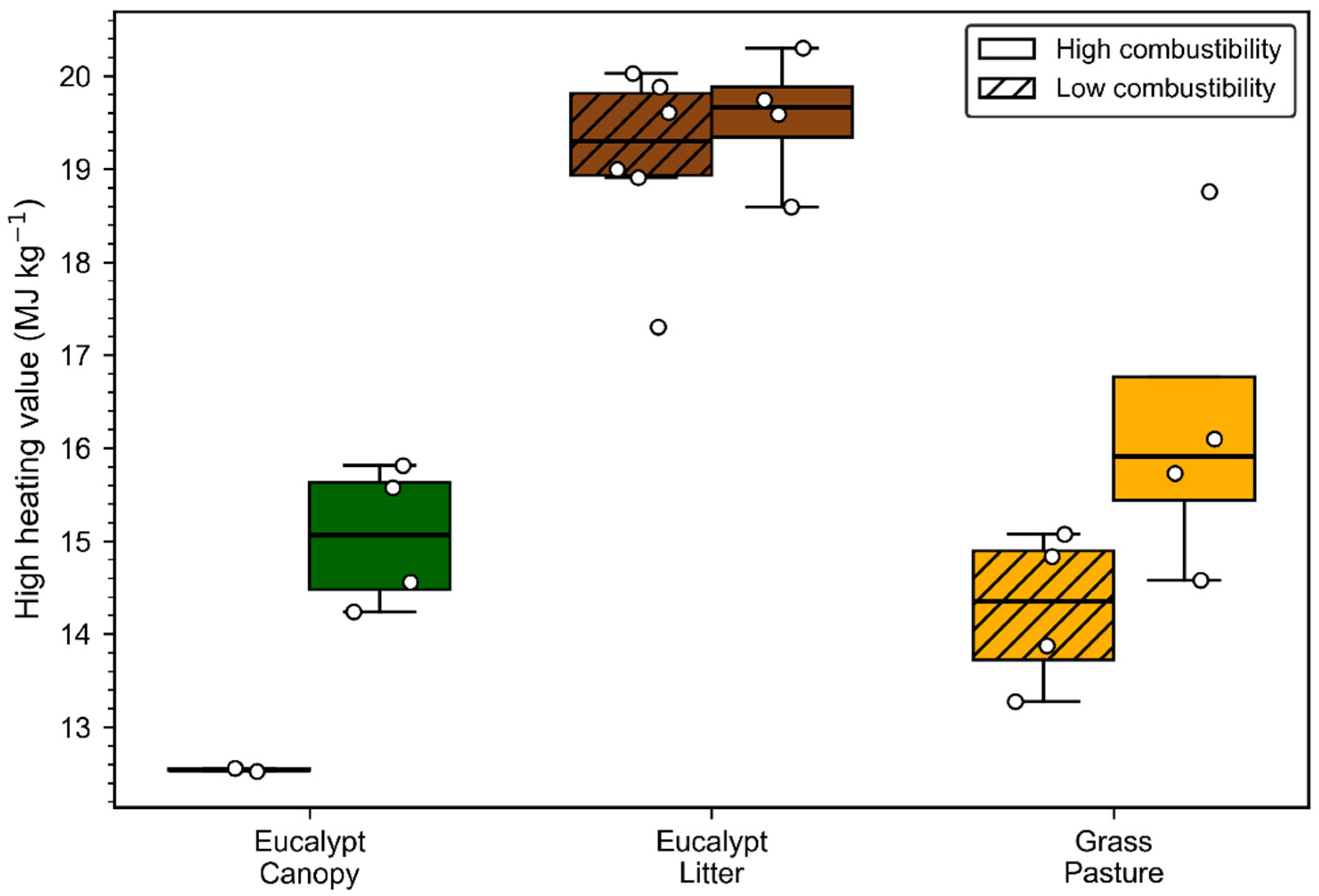
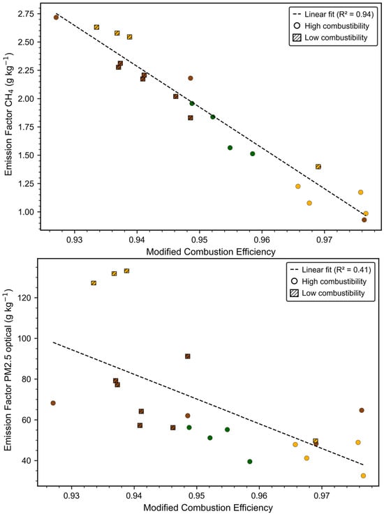
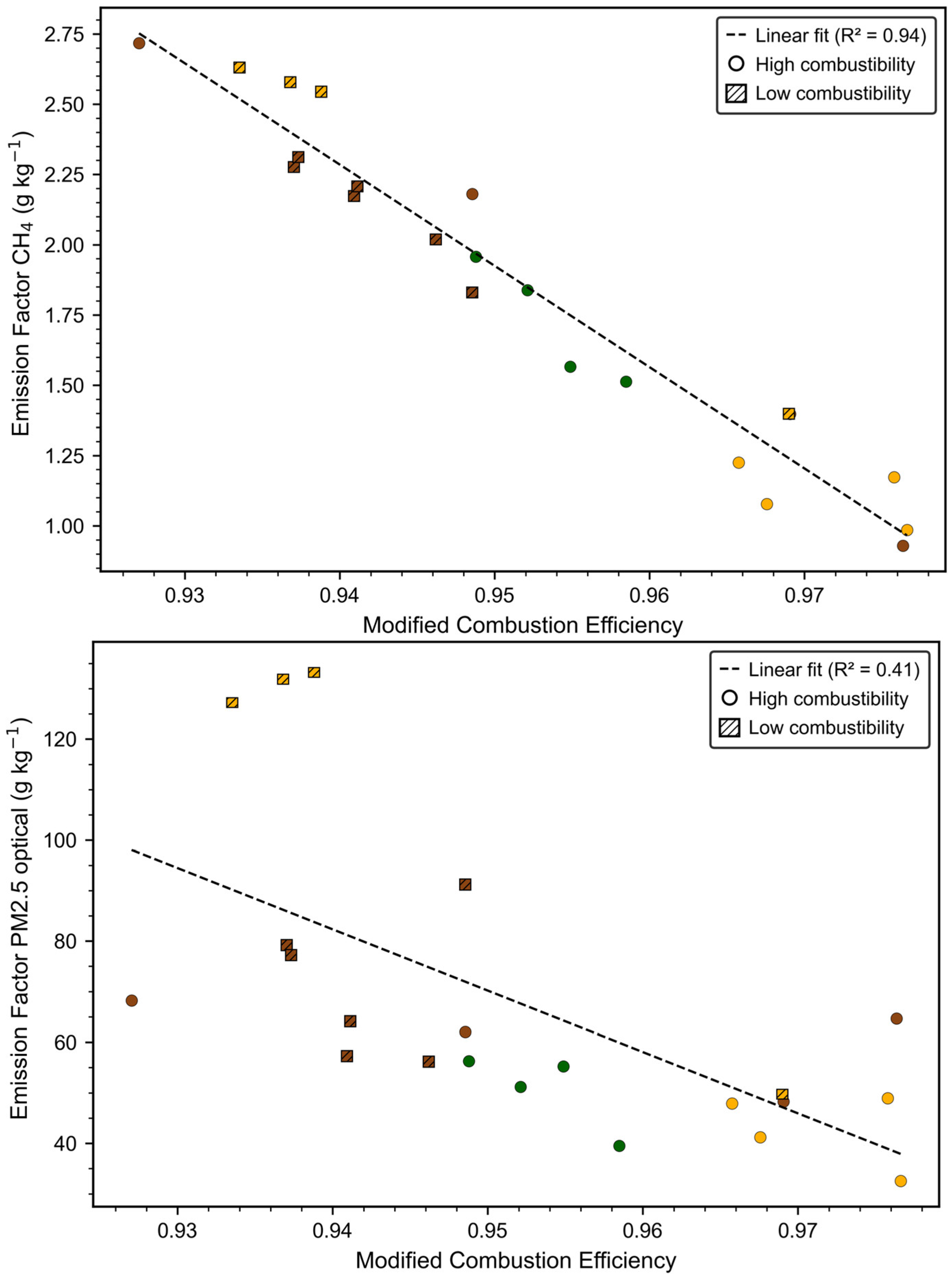
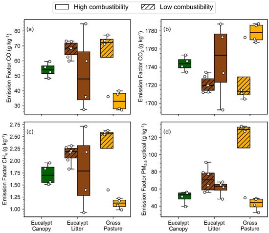
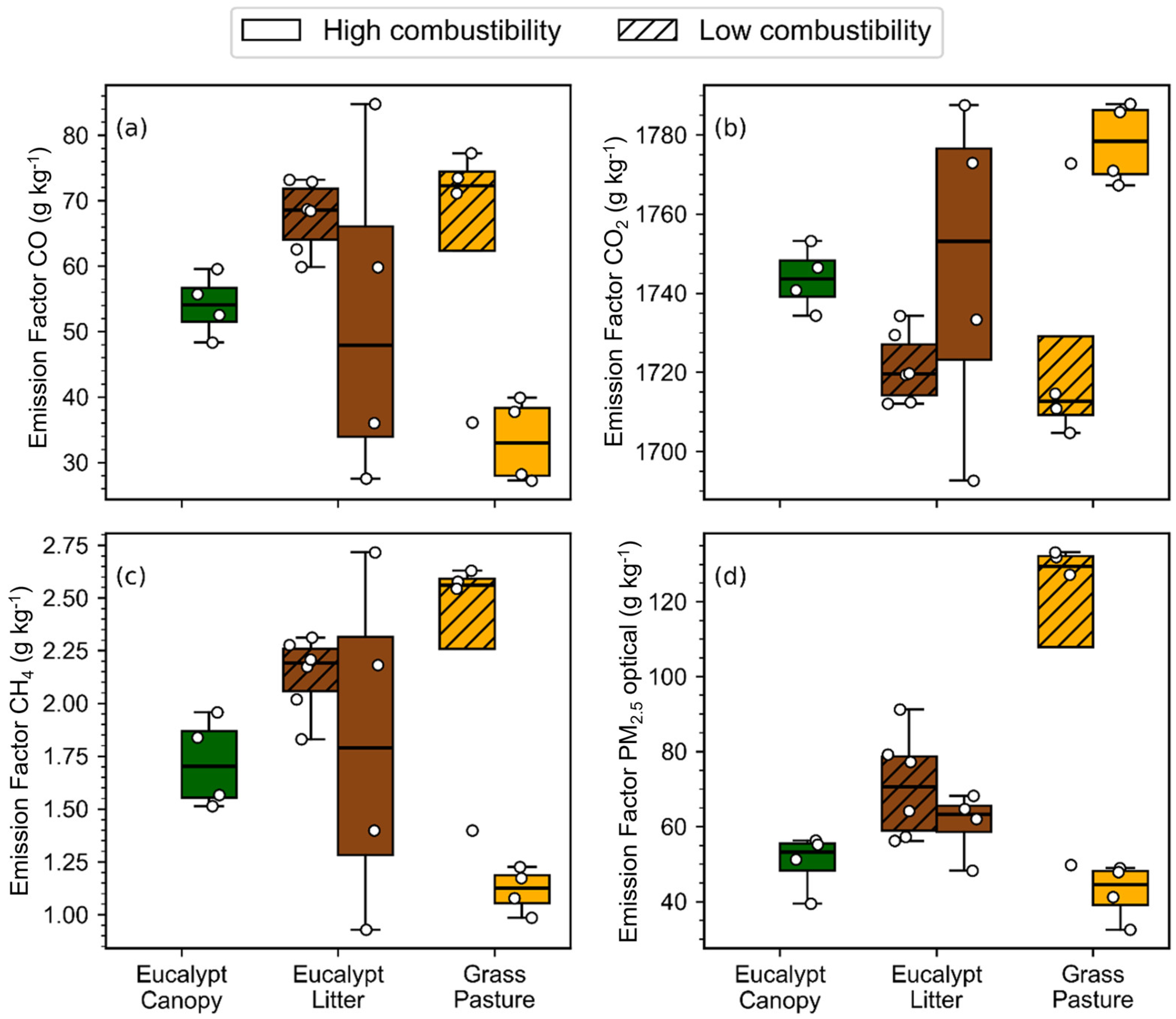
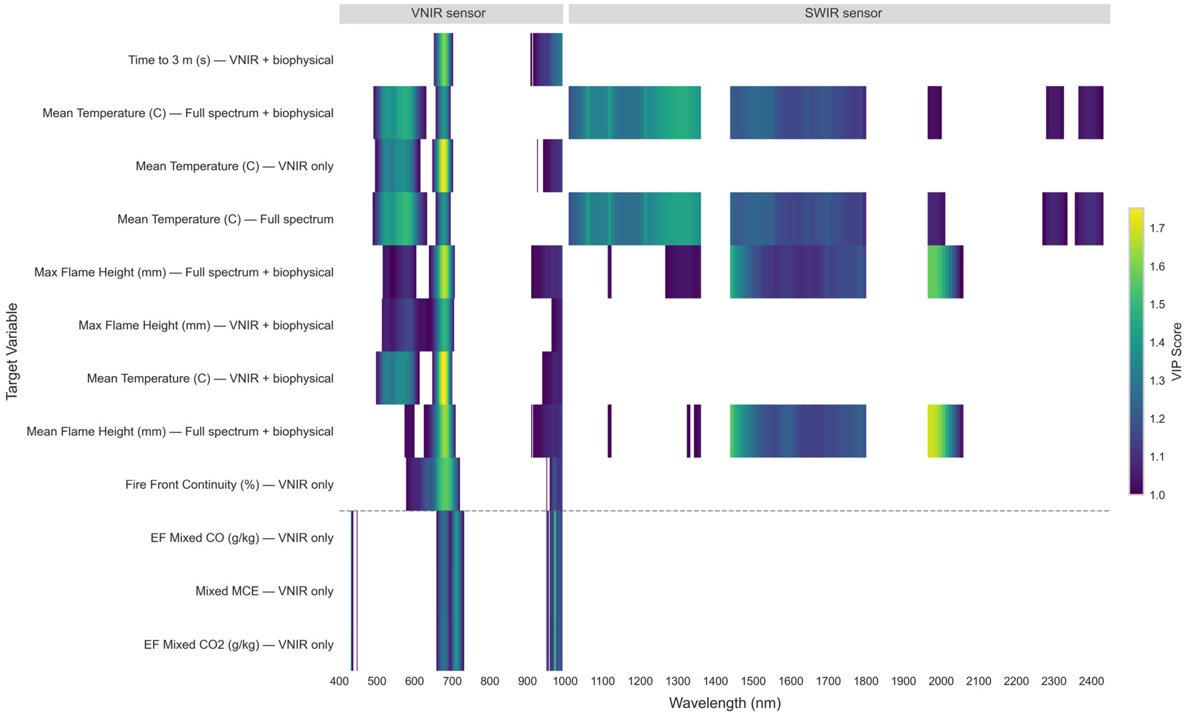

Disclaimer/Publisher’s Note: The statements, opinions and data contained in all publications are solely those of the individual author(s) and contributor(s) and not of MDPI and/or the editor(s). MDPI and/or the editor(s) disclaim responsibility for any injury to people or property resulting from any ideas, methods, instructions or products referred to in the content. |
© 2026 by the authors. Licensee MDPI, Basel, Switzerland. This article is an open access article distributed under the terms and conditions of the Creative Commons Attribution (CC BY) license.