


Highlights
What are the main findings?
- Supervised semantic segmentation applied to OCT image stacks to identify material layer interfaces.
- Seamless registration and stitching of image stacks via interface-based alignment and blending.
What are the implications of the main findings?
- Automated pixel-wise computation of paint layer thickness.
- A new workflow for OCT post-processing to extend the stratigraphic characterization of paintings to macroscopic fields of view.
Abstract
Non-invasive characterization of painting stratigraphy is challenged by light attenuation in optically heterogeneous opaque materials composing micrometric layers. Optical coherence tomography (OCT) provides suitable, non-invasive, depth-resolved imaging capabilities; however, large-area stratigraphic analysis is limited by the restricted field of view of individual stacks, high data dimensions, and the lack of robust methods for stitching volumes acquired at different focal depths. In addition, conventional layer thickness estimation relies on manual identification of intensity peaks along A-scans, which is time-consuming, operator-dependent, and unsuitable for large-scale analysis. Building upon our prior work, which introduced an AI-enhanced method for OCT volume analysis, we present an automated workflow integrating supervised semantic segmentation, volumetric mosaic stitching, and pixel-wise layer thickness quantification. OCT B-scans are segmented using a Random Forest classifier within the Trainable Weka Segmentation framework to delineate material interfaces. Adjacent OCT volumes are then combined into a continuous mosaic, and interfacial distances are computed using a custom MATLAB routine to obtain pixel-wise thickness measurements over extended fields of view. The model discriminates air/paint and paint/primer interfaces with an accuracy ranging from 96.4% to 97.1% and a weighted average F1-score exceeding 0.95, enabling quantitative reconstruction of paint thickness with micrometric resolution. This method enables efficient and reproducible analysis of large OCT datasets, extends stratigraphic characterization to macroscopic fields of view while maintaining micrometric resolution, and reduces processing time while improving consistency compared to manual approaches.
1. Introduction
The acquisition of large-scale and high-resolution three-dimensional (3D) information by optical microscopy is a relevant challenge in several diagnostic applications. In the field of cultural heritage (CH), non-invasive techniques are required to investigate the stratigraphy of multilayered artworks, such as paintings, over macroscopic areas extending across several millimeters while maintaining micrometric lateral and axial resolution. Such analyses are essential for the morphological characterization and thickness evaluation of heterogeneous superimposed layers and for monitoring ageing phenomena or conservation-induced modifications over time. However, the non-invasive cross-sectional investigation of paintings is often hindered by the presence of optically opaque materials, such as pigments, which strongly limit light penetration within the sample.
Among the optical techniques proposed for this purpose, optical coherence tomography (OCT) has become one of the most established methods for non-invasive and depth-resolved imaging. Originally developed for ophthalmology, OCT provides high-resolution cross-sectional images based on the detection of backscattered near-infrared (NIR) radiation and enables the visualization of internal interfaces associated with local refractive-index variations. In CH diagnostics, OCT performance may be affected by highly scattering or absorbing pictorial layers [1]. Nevertheless, the technique has proven particularly effective for the evaluation of varnish thickness and has been successfully applied to real-time monitoring of cleaning procedures [2,3].
Large-scale stratigraphic analysis by OCT is limited by several technical challenges. These include the restricted field of view (FOV) of individual volumetric acquisitions and the absence of robust approaches for mosaicking image volumes acquired at different focal depths; the lack of accurate, fast, and representative procedures for layer thickness estimation, which often still rely on the manual identification of intensity peaks along A-scans; and the large size of OCT datasets, which requires computational platforms with high processing and storage capabilities.
A common strategy for extending the effective imaging FOV consists of acquiring multiple contiguous and partially overlapping image stacks at high magnification and combining them into a single composite dataset while preserving the native spatial resolution. This mosaicking, or stitching, procedure requires reliable image-registration and blending algorithms to generate seamless volumetric reconstructions. The main challenge is associated with the management of signal-intensity variations and geometric misalignments, particularly when image volumes are acquired at different focal depths. Although motorized translation stages provide high positioning precision, the recorded stage coordinates are generally insufficient to ensure accurate pixel-level reconstruction of the entire dataset [4].
Over the last two decades, several methods for stitching 2D and 3D images have been developed, mainly in the biomedical field. The stitching workflow generally consists of two main steps: image registration, based on pixel-intensity variations and/or homologous feature recognition [5], and blending of overlapping regions through linear or non-linear approaches [6]. Intensity-based registration commonly relies on cross-correlation methods [7], whereas feature-based approaches exploit scale- and rotation-invariant image patterns [8]. Hybrid methods combine Fourier transform-based phase correlation for overlap estimation with global least-squares optimization and non-linear blending [4]. To reduce autocorrelation artifacts that may compromise alignment accuracy, the use of discrete Laplacian operators has also been proposed [9]. Other approaches generate en face projections from OCT volumes and apply computer-vision algorithms to identify common features within overlapping regions [10].
In the context of heritage science, only a limited number of studies have addressed large-scale OCT imaging through volumetric stitching. Zhou et al. proposed an adaptive stitching algorithm based on cross-correlation analysis to identify optimal overlap between adjacent 3D OCT datasets and reduce redundancy artifacts [11]. However, axial variations of the OCT focal position were not considered, resulting in visible artifacts in the reconstructed volumes. Callewaert et al. introduced a physics-based stitching method combining graph-based segmentation with attenuation-coefficient-guided refinement [12,13]. During acquisition, the sample surface is tracked to maintain focus across large scanning areas, while post-processing aligns adjacent scans by estimating axial displacements from segmented interfaces. This approach assumes different optical attenuation coefficients between neighboring layers; consequently, segmentation errors may arise when adjacent layers exhibit similar attenuation properties.
More recently, deep-learning (DL) approaches have been introduced to automate the stitching process [14]. These methods include end-to-end registration networks that jointly learn alignment and fusion, replacing conventional multi-step pipelines [15,16]; sliding-window classifiers for local block-merging decisions in large 3D datasets [17]; and learned feature detector/matcher frameworks that improve tile-to-tile registration robustness under low contrast, repetitive textures, and microscopy artifacts [18]. Additional approaches integrate segmentation- or graph-guided strategies to improve the global consistency of stitching seams [19].
The main advantage of DL-based methods lies in their ability to estimate dense correspondences between image datasets through convolutional neural networks (CNNs) and to perform structure-aware registration by segmenting relevant anatomical or morphological features prior to alignment. Specifically, U-Net-based architectures enable registration on segmented masks or skeletonized structures rather than directly on raw intensity data, improving robustness and alignment accuracy.
To quantify the thickness of material layers in paintings by OCT, measurements are still frequently performed manually by identifying intensity peaks along individual A-scans corresponding to material interfaces [20,21]. Since a single OCT volume may contain hundreds of B-scans, manual analysis is time-consuming, operator-dependent, and unsuitable for obtaining statistically representative thickness measurements over extended areas. Moreover, this procedure is highly sensitive to noise and unreliable under low-contrast conditions.
AI-based segmentation methods provide an effective alternative for stratigraphic analysis by automatically partitioning OCT images into regions associated with different material layers [13,22,23,24]. In biomedical imaging, DL models such as CNNs [25], fully convolutional networks (FCNs) [26], and recurrent neural networks (RNNs) are widely employed for this purpose, often combined with graph-based optimization or shortest-path algorithms to refine interface localization [27,28,29]. Most approaches adopt an encoder–decoder architecture derived from the U-Net model and its variants, which remain the reference standard for biomedical image segmentation [30,31,32,33]. These models are generally trained on large, annotated datasets in which ground-truth segmentations are manually defined by domain experts.
Although AI-based image-processing methods have become widely adopted in biomedical imaging, their application in heritage science remains comparatively limited. This is generally due to the need for programming expertise, complex hardware and software configurations, and access to high-performance computing resources [34]. To address these limitations, several open-access platforms with cloud-based or simplified graphical interfaces have been developed, enabling non-programmer users to train and deploy DL models without writing code [35]. Despite these advances, important challenges remain, including the complexity and heterogeneity of imaging datasets, the absence of unified frameworks for specific applications such as microscopy-image stitching, and the need for reliable data management and reproducibility strategies [36].
To address these limitations, in our previous work [37], we introduced an automated workflow based on supervised machine learning (ML)-based semantic segmentation of OCT B-scans for the robust identification of material interfaces and quantitative layer thickness estimation across entire datasets. Building on this approach, the present work extends the methodology to enable both automated stitching of contiguous OCT volumes and pixel-wise thickness quantification over large fields of view. OCT B-scans are segmented using a Random Forest (RF) classifier [38] implemented within the Trainable Weka Segmentation (TWS) framework [39,40,41] to identify material interfaces. The TWS framework offers an intuitive environment for manual annotation and feature selection, facilitating iterative refinement of the classifier without requiring advanced programming expertise. The RF classifier provides a favorable trade-off between segmentation accuracy, computational efficiency, and robustness while avoiding the reliance on extensive annotated training datasets typically required by deep learning approaches. The resulting classified image stacks are processed through a custom computational routine to estimate stitching parameters, which are subsequently applied to reconstruct continuous mosaicked OCT volumes from partially overlapping acquisitions. Interfacial distances are then computed to generate pixel-wise thickness maps over the stitched dataset.
By reducing data complexity while preserving micrometric spatial resolution, the proposed workflow enables efficient, reproducible, and statistically representative analysis of large OCT datasets. The method extends stratigraphic characterization to macroscopic areas and significantly improves processing speed and consistency compared with conventional manual procedures.
2. Materials and Instrumentation
2.1. Samples
Two acrylic paints (extra-fine acrylic colors; Maimeri Brera™, Milan, Italy), both transparent in the NIR range and commonly used in artistic applications, were selected to validate the proposed method. The first was Primary Red Magenta (PRM; commercial code PV19-73900, composed of quinacridone (C20H12N2O2). The second was Lemon Yellow (LY; commercial code PY175-11784), based on benzimidazolone (C7H4N2O).
Using these paints, two samples simulating real paintings with varying layer configurations were prepared (Figure 1):
Figure 1.
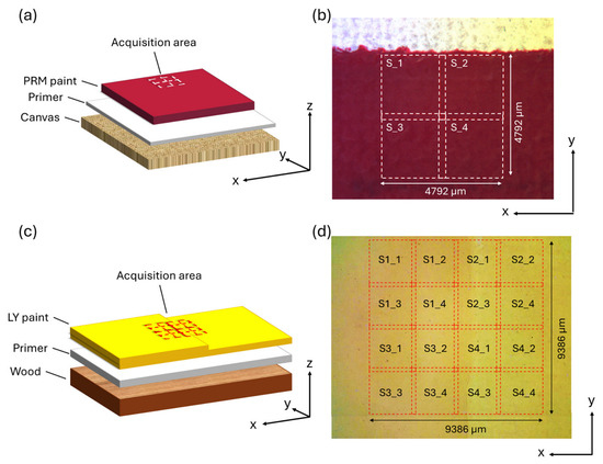
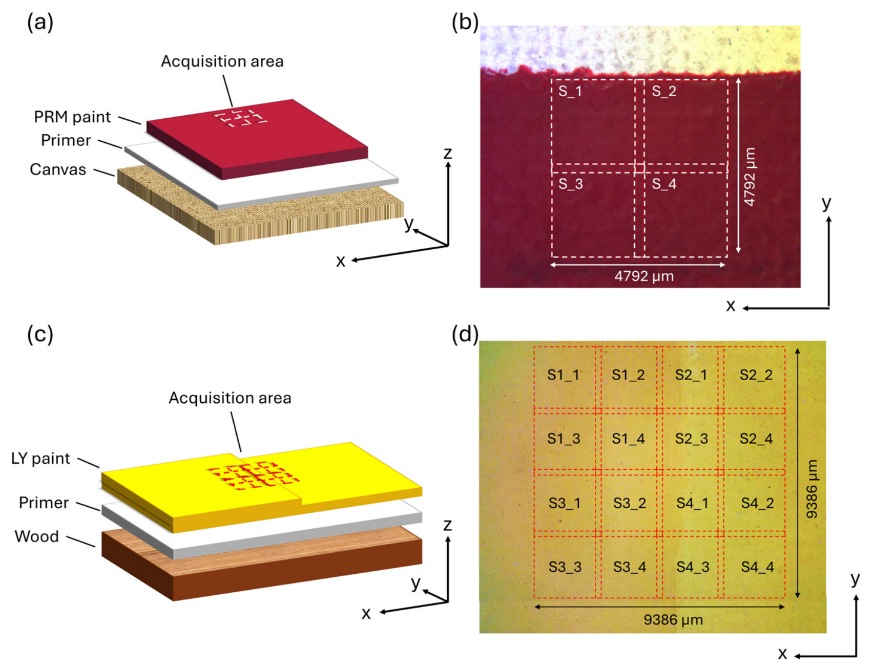
Schematic representation and bright-field image of the field of view (FOV) of the analyzed samples: PRM on canvas (a,b) and LY on wood (c,d). The OCT measurement areas are indicated by the dashed squares. The stacks (S) are arranged in groups of four (2 × 2 matrix) and numbered from 1 to 4 within each group.
- LY on wood (Figure 1c): LY was applied onto a wooden substrate, pre-treated with the Lefranc Bourgeois™ acrylic primer, to form two adjacent areas (approximately 1 cm2 each) of different thicknesses. A 50 ± 5 µm Kapton tape (DuPont™, Wilmington, DE, USA) served as a spacer and thickness reference by applying one or two stacked layers to achieve the target thicknesses. The paint was spread with a glass spatula to ensure uniformity. Sixteen partially overlapping OCT volumes were acquired across the transition between the ~50 µm and the ~100 µm regions (Figure 1d).
2.2. OCT Device and Measurements
Cross-sectional imaging was performed using a commercial spectral-domain optical coherence tomography (SD-OCT) system, a Telesto-II (Thorlabs Inc., Newton, NJ, USA). The platform is equipped with a superluminescent diode (SLD) source centered at 1300 nm and an approximate spectral bandwidth of 100 nm, resulting in an axial resolution of 5.5 μm in air. The system used an objective lens with an effective focal length (EFL) of 36 mm, providing a lateral resolution of 13 μm, a FOV of 10 × 10 mm2, and a maximum imaging depth of 3.5 mm.
The detection unit comprises a spectrometer based on a diffraction grating and a high-speed line-scan camera, with a 76 kHz maximum acquisition rate. Depth-resolved reflectivity profiles (A-scans) were reconstructed by fast Fourier transform (FFT) of the acquired spectral interferograms. The scanning probe was mounted on high-precision motorized XY translation stages with rotational capability. Coarse axial adjustment of the probe head was used for sample positioning and focus optimization.
OCT volumes were acquired as a set of four, arranged in a 2 × 2 matrix configuration, with an overlap of 200 µm along both the x- and y-axes. For the PRM sample, four stacks (2.5 × 2.5 × 0.6 mm3) were collected to obtain a final reconstructed volume of 4.8 × 4.8 × 0.6 mm3 (Figure 1b). For the LY sample, sixteen stacks (2.5 × 2.5 × 0.5 mm3) were acquired to obtain a mosaic volume of 9.4 × 9.4 × 0.5 mm3 (Figure 1d). For all OCT datasets, the voxel size was 3.55 μm3.
For all acquisitions, the lateral overlap was controlled by software through predefined x–y stage shifts, whereas the focus depth along the z-axis was manually adjusted based on the paint–air interface, without quantification of the axial displacement.
3. Methods
3.1. Workflow
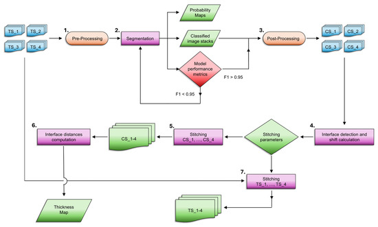
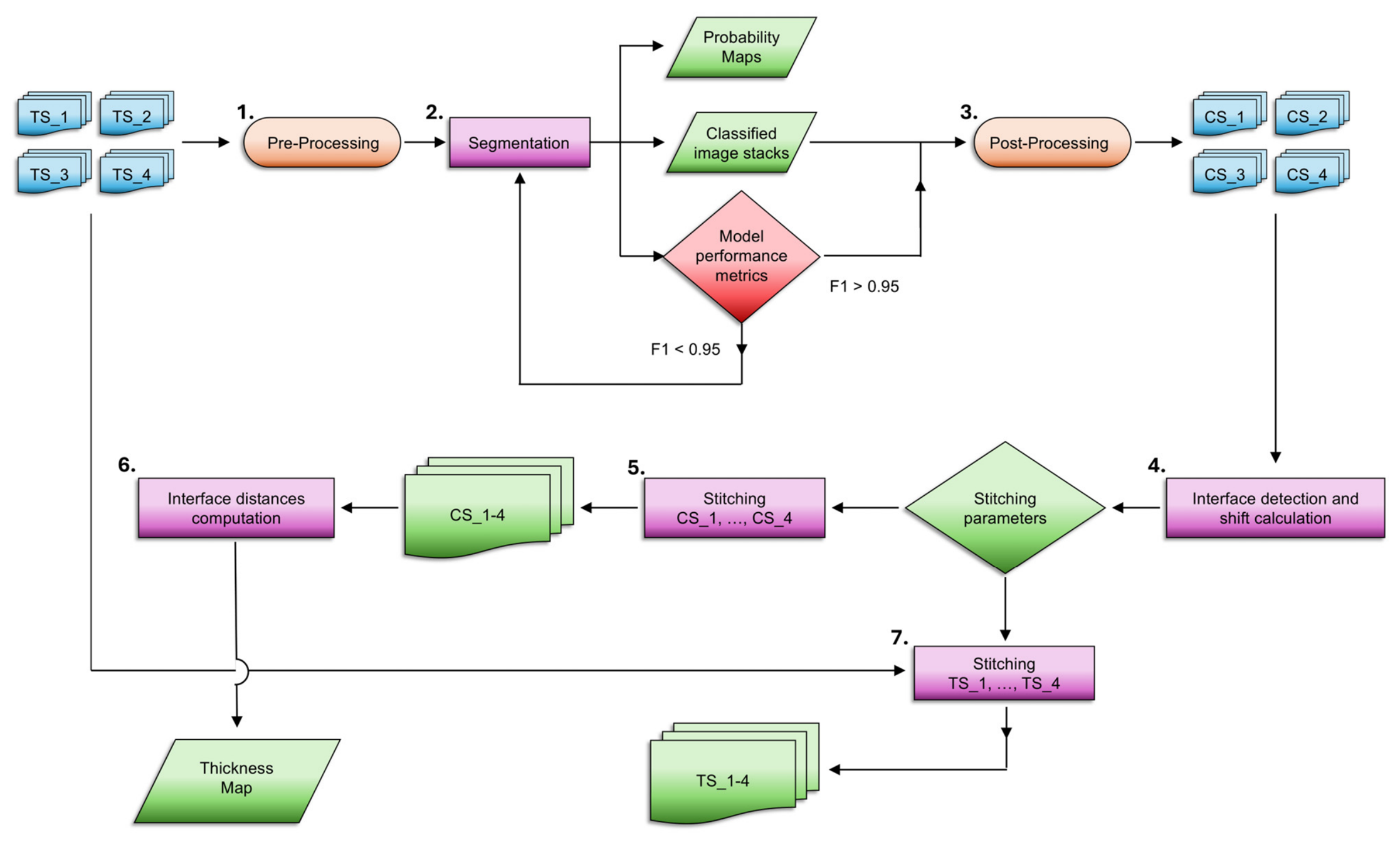
The proposed workflow is illustrated in Figure 2 and consists of seven main steps, which are described in detail in the following sections:
Figure 2.
Schematic of the automated workflow for segmenting OCT images (TS_1, …, TS_4), calculating the parameters for stitching the classified image stacks (CS_1, …, CS_4 → CS_1-4), computing the layer thickness (thickness map), and stitching the original OCT volumes (TS_1-4).
- Acquisition of the original tomographic image stacks (TS_1, …, TS_4) with a motorized stage for precise overlapping, and pre-processing in ImageJ (version 1.54p).
- Segmentation within an iterative supervised learning framework (Trainable Weka Segmentation, TWS) integrated in the Fiji environment (version 1.54p), consisting of sequential training and model refinement guided by visual inspection and probability-based quality control. The classifier training was iteratively refined until convergence was achieved, defined as F1 score > 0.95 (harmonic mean of precision and recall).
- Post-processing of the resulting classified stacks (CS_1, …, CS_4) using denoising filters and outlier removal in ImageJ.
- Automated interface detection and shift calculation on all classified image stacks in MATLAB R2024b (MathWorks, Natick, MA, USA) to obtain the stitching parameters.
- Stitching of the classified image stacks to obtain the classified mosaic (CS_1-4).
- Automated calculation of interface distances of CS_1-4, yielding the overall thickness map (MATLAB).
- Stitching of the original tomographic volumes, using the previously estimated stitching parameters, to obtain the tomographic image mosaic TS_1-4 (MATLAB).
3.2. Supervised Image-Stacks Segmentation
Prior to segmentation, the original tomographic volumes were preprocessed in ImageJ. This included rescaling the image stacks to their physical dimensions and applying intensity adjustments (brightness and contrast). The latter were determined by visual inspection of a representative subset of B-scans and then uniformly applied to the entire dataset to reduce artifacts that could hinder interface detection by the classifier. Since all images were acquired under fixed illumination conditions and displayed largely homogeneous texture, a single set of adjustment parameters could be applied consistently across the entire dataset. No additional smoothing or denoising algorithms were applied.
Manual annotation of the images was performed at the pixel level by tracing the boundaries between material layers using the freehand or segmented line selection tools. Two classes were defined (class 1: interfaces; class 2: background), where the background included pixels corresponding to the bulk of the material layers or air. The number of classes was intentionally kept to a minimum to reduce training time while preserving classification efficiency. Pixel-wise annotations were performed on randomly selected images to train the model to distinguish apparent discontinuities due to signal loss or artifacts from true discontinuities.
The fast Random Forest classifier used for segmentation was implemented as a multithreaded RF with 200 trees and two randomly selected features per node. The classifier combines multiple decision trees, each built on random subsets of the training data, and aggregates their predictions to obtain the final result. The training process begins with bootstrap sampling (sampling with replacement) to create subsets of the original dataset. Decision trees are then constructed by selecting random feature subsets at each node for splitting. Final predictions are made by majority voting among all trees, with node splitting typically based on the Gini impurity index [38].
To improve the classification process, several feature filters available in TWS were applied. These included edge detectors (Sobel, Hessian, and Difference of Gaussian filters) to enhance object boundaries, membrane detectors (Membrane Projection) to localize structures with a specified thickness and size, and a noise-reduction filter (Gaussian blur). The membrane detector parameters were set as follows: thickness = 1 pixel, patch size = 19 pixels, minimum sigma = 1 pixel, and maximum sigma = 16 pixels.
Sequential training was guided by visual inspection of segmentation outputs, manual correction of misclassified pixels, and incremental expansion of the training set, improving robustness, particularly at interface discontinuities and in regions where bulk pigment grains were misclassified. Probability maps were generated to provide pixel-wise confidence estimates and support both refinement and quality control. The training was performed independently for PRM and LY samples, and the respective models’ performances were evaluated in the Weka environment. The evaluation was conducted using 10-fold cross-validation: in each case, the dataset was partitioned into ten subsets, with iterative training and validation such that each subset served once as test data, while the remaining subsets were used for training. Metrics, including accuracy, precision, recall, F1-score, confusion matrix, Receiver Operating Characteristic (ROC), and Precision–Recall Curve (PRC)-based measures, were computed by averaging over folds. The F1-score was used as the primary performance metric.
Finally, the segmented image stacks were post-processed in ImageJ. This included (i) outlier removal using a selective filter, which replaces a pixel with the median of its surrounding pixels if it deviates from the median by more than a specified threshold (50), with the neighborhood defined by a radius of 0.5 pixels, and (ii) conversion of the images to 8-bit binary masks, where class 1 and class 2 are represented by white (255) and black (0), respectively. This last step significantly reduced the data size while maintaining all the required information.
All procedures were performed on a workstation with 768 GB RAM and a 2.70 GHz processor, requiring approximately three hours per group of four stacks. This hardware specification pertains to the experimental setup and does not constitute a strict requirement of the proposed method, which can be adapted to lower-memory environments through partitioned (block-wise) processing.
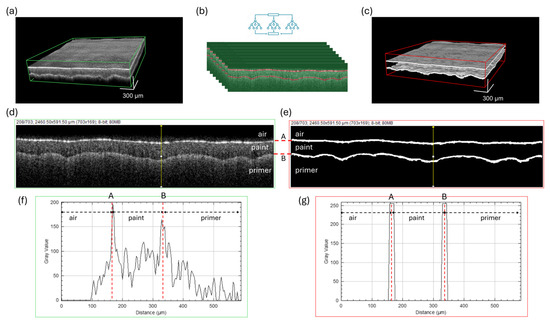
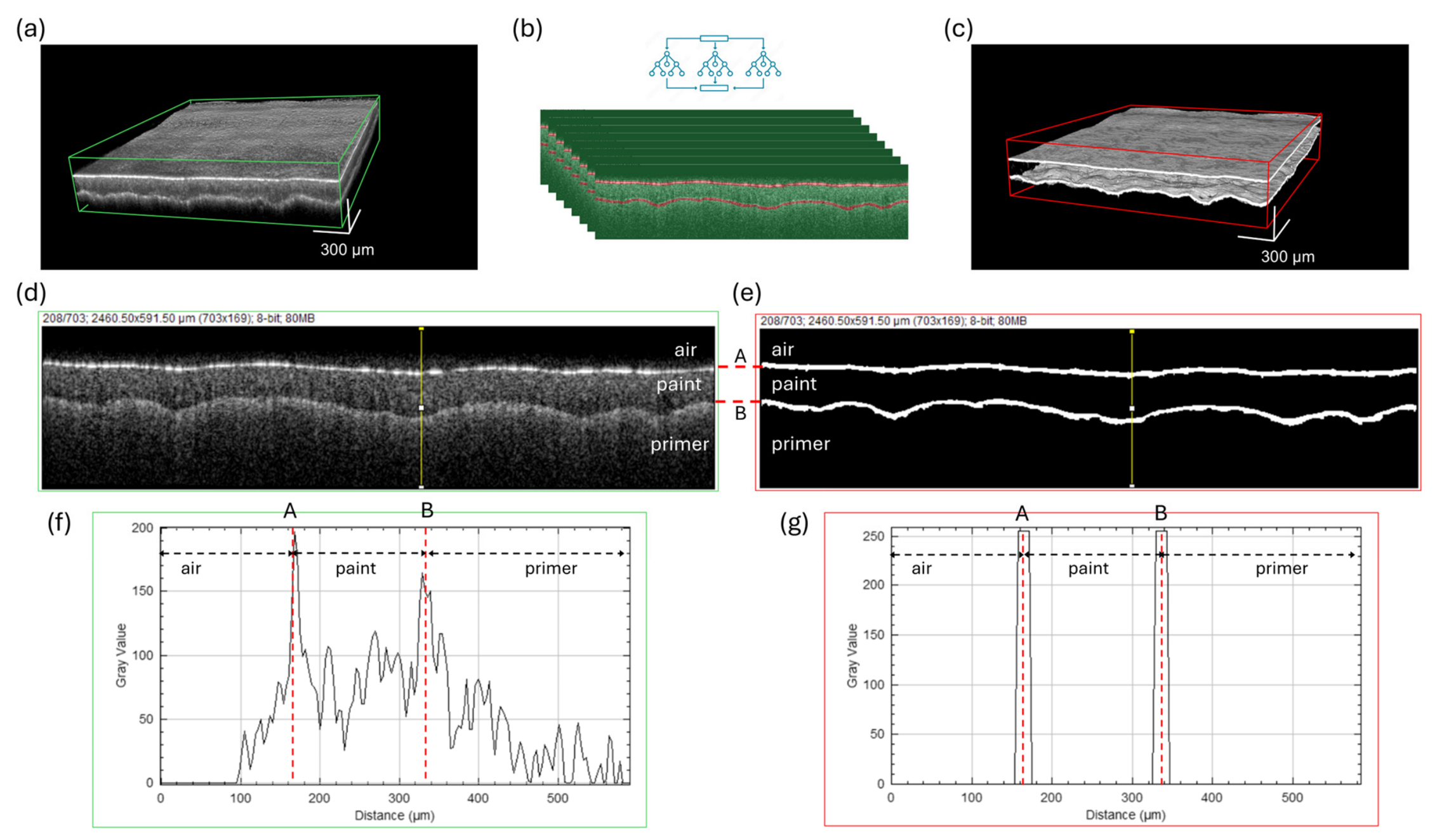
The main steps of the procedure are illustrated in Figure 3 for the stack CS_2 of the PRM sample, as an example. The OCT image stack (a) is manually annotated by defining two class labels (class 1, interfaces, shown in red; class 2, background, shown in green) and is then used to train the RF classifier (b). The trained model is subsequently applied to generate the classified image stack, resulting in a binary segmentation mask (c). Representative B-scans (slice 208 of 703) extracted from the original OCT volume (d) and the corresponding classified stack (e) demonstrate the classifier’s effectiveness in identifying interface A (air/paint) and interface B (paint/primer). Finally, the corresponding depth-intensity (Z) profiles show that the peaks in the raw OCT signal (f) are clearly isolated after the classification procedure (g), enabling the accurate quantification of the paint layer thickness.
Figure 3.
OCT data segmentation workflow: (a) original image stack; (b) schematic representation of the RF classifier (light blue) applied after manual annotation, where the two training classes are defined as interfaces (red) and background (green); (c) resulting binary segmentation mask; (d) representative B-scan from the original OCT volume and (e) its corresponding classified result, indicating interface A (air/paint) and interface B (paint/primer)—the yellow lines indicate where the Z-profiles were extracted; depth-intensity (Z) profiles (f) before and (g) after classification, demonstrating the isolation of signal peaks.
3.3. Stitching Procedure
All image registration and stitching were performed in MATLAB using custom scripts to combine four volumetric datasets (classified stacks CS_1–CS_4) into a continuous three-dimensional reconstruction. The system coordinates X, Y, and Z correspond to the lateral, stacking, and depth directions, respectively. Each dataset was treated as a discrete volume , where .
3.3.1. Interface Detection
To support robust alignment, two interfaces (A: upper, B: lower) were automatically extracted from each binary image set. For each spatial position (x, y), foreground white pixels (intensity, I = 255) along the depth axis were identified as:
Contiguous clusters of pixels along z were detected, and only positions exhibiting exactly two clusters were retained. The interface locations were computed as the centroid of each cluster, yielding interface maps (x, y) and (x, y).
3.3.2. Lateral Alignment and Stitching
The volumes were first stitched pairwise (CS_1-2 and CS_3-4) along the lateral X-direction. To correct vertical misalignment, a relative Z-shift between adjacent stacks was estimated using the mean axial position of interface A at the contact boundaries (a, b):
where is the total number of A-scans along the -direction at the contact boundaries. After applying the estimated shift, adjacent volumes were merged using an overlap (56 pixels = 200 µm, pixel size = 3.55 µm) along X. To ensure smooth intensity transitions within the overlap region, voxel intensities were combined using a cosine-weighted blending function. A normalized coordinate was defined across the overlap, and the blending weight was expressed as:
The blended intensity is given by:
where and denote the two overlapping portions of each stack, with varying smoothly from 0 (fully ) to 1 (fully ).
The blending produced intermediate grayscale values in the overlap region due to the weighted averaging of foreground (255) and background (0) voxels. These values were subsequently binarized using a fixed threshold (intensity > 127, the midpoint of the 8-bit intensity range), restoring a binary representation of the reconstructed volume, which was functional to the later thickness computation step.
3.3.3. Alignment of Row1 and Row2 and Final Volume Reconstruction
The two intermediate mosaics, Row1 and Row2, were subsequently aligned along the stacking direction Y. Interface detection was repeated to obtain updated interface maps, and the relative displacement was estimated within the overlapping region along Y (56 slices = 200 µm) using interface A, following the same averaging approach described above.
After applying the estimated shift to Row2 along Z, the final volume (CS_1-4) was reconstructed by concatenating the non-overlapping portion of Row1, blending overlapping regions along Y using the same cosine weighting formulation, and appending the remaining portion of Row2. A final binarization step was applied to all slices.
3.3.4. Alignment and Volume Reconstruction of OCT Image Stacks
The relative Z-shifts along both the X- and Y-directions, which were precisely quantified through the overall stitching of the classified image stacks, correspond to the displacement of the focal depth manually adjusted for each acquisition during OCT measurements. Knowing these values allowed stitching of the tomographic stacks (TS_1–TS_4), bypassing the identification of the interface position, which is only applicable to segmented binary images. This procedure was implemented using a dedicated MATLAB script and involved the same pairwise stitching along the lateral X-direction described above to generate Row1 and Row2. These intermediate volumes were subsequently stitched along the Y-direction, using the same cosine-weighted blending approach within the 56-pixel overlapping region, resulting in a smoothly assembled final OCT volume.
3.4. Automated Layer Thickness Computation
Material layer thickness was quantified from the reconstructed mosaic of classified image stacks using a custom MATLAB script. Interface detection followed the procedure described in Section 3.3.1, whereby for each column of each B-scan, two contiguous regions of foreground pixels (value 255) were identified, separated by the largest gap along the z-axis. Columns not exhibiting two distinct interfaces were excluded from the analysis.
For each interface, the representative position was defined as the mean pixel location of all pixels within the corresponding cluster, providing a single value per column. The local layer thickness was then computed as the absolute difference between the central positions of interfaces A and B for each column. Pixel-based distances were converted into physical units using the known pixel size (3.55 µm).
Outliers in the resulting distance matrix were corrected using local neighborhood averaging using a 5 × 5 pixel window (±2 pixels in both directions), ensuring spatial consistency of the measurements. Statistical descriptors, including mean, standard deviation, and variance, were computed from all valid thickness values.
Spatial variability was visualized using 2D and 3D thickness maps generated from the reconstructed dataset. A perceptually uniform colormap was used to ensure proportional mapping between thickness variations and color changes, minimizing visual bias. The overall distribution of thickness values was further assessed using histograms to evaluate layer uniformity across the dataset.
For the conversion from optical to geometric thickness, a refractive index of n = 1.5 was employed as a representative mean value for paint layers. Although n is known to depend on the specific paint composition, adopting a constant value ensures a uniform reference for thickness estimation across the entire dataset. Consequently, the geometric thicknesses reported herein are to be interpreted as approximations of the true absolute thickness, whereas relative differences and intra- and inter-dataset comparisons are preserved without bias.
4. Results
4.1. Primary Red Magenta (PRM) on Primed Canvas
4.1.1. Classified Image Stitching
For the PRM sample, the classifier was initially trained on the first stack and subsequently updated using incremental learning by progressively incorporating pixel-wise annotations from the remaining stacks into the training set. This resulted in a converged model, whose performance was evaluated in the Weka environment. The overall classification metrics, the confusion matrix, and class-wise accuracies are reported in Table 1. A total of 460,886 pixels (instances) were manually annotated across the complete training dataset, of which 60,435 corresponded to interface pixels and 400,451 to background pixels. While this total is roughly equivalent to the area of four full B-scans, the annotations were sparsely distributed over multiple images and not confined to a limited set of frames. Given that the four stacks combined comprise 703 B-scans each of 703 × 169 pixels, for a total of approximately 334 million pixels, the annotated fraction amounts to about 0.14% of the entire dataset.
Table 1.
Performance metrics of the classifier for the segmentation of the PRM image stacks.
The model accurately discriminates the air/paint and paint/primer interfaces (class 1) from non-interface regions, including air and bulk material (class 2), achieving 97.1% correctly classified instances (pixel-wise), with only 2.9% misclassifications. The confusion matrix indicates strong performance for class 2 (397,491 true negatives), while reduced sensitivity is observed for class 1. Despite this lower sensitivity, the model maintains robust overall performance, as confirmed by the high Matthews Correlation Coefficient (MCC) (0.868), the Receiver Operating Characteristic (ROC) area (0.992), and Intersection over Union (IoU), which further quantifies the spatial overlap between predicted and reference regions. The class-wise IoU values are 0.789 and 0.967 for class 1 and class 2, respectively. This indicates reliable class separability and stable predictive behavior. Given the weighted average F1-score (>0.95), the trained model was used for the segmentation of all four stacks.
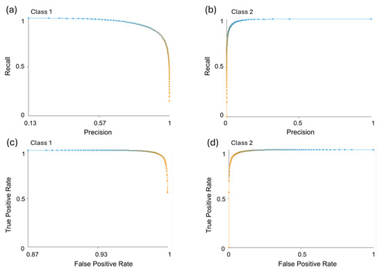
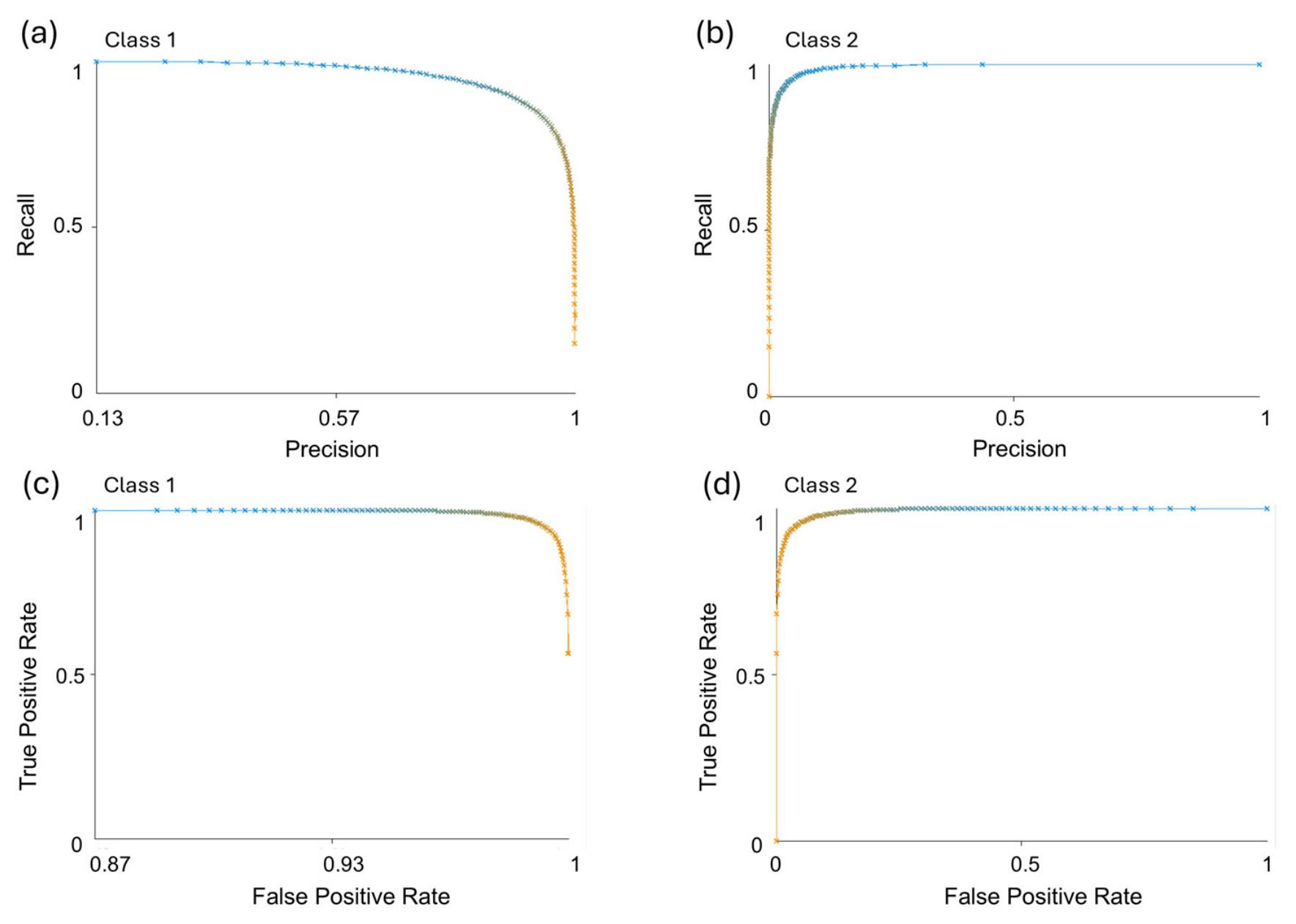
Figure 4 summarizes the model performance in terms of precision–recall and ROC analysis. The precision–recall curves for class 1 (a) and class 2 (b) show that most operating points lie in the upper-right region, indicating a favorable precision–recall trade-off across thresholds. The F1 score reaches 0.882 for class 1 and 0.983 for class 2, consistent with Table 1. The ROC curves in Figure 4c,d yield an area under the curve (AUC) of 0.992 for both classes, confirming the strong and stable discriminative capability of the classifier.
Figure 4.
Classifier performance evaluation. Precision/recall curves for (a) class 1 (interfaces) and (b) class 2 (non-interface regions). ROC curves for (c) class 1 and (d) class 2. Data points are clustered in the upper-right quadrant of the precision–recall plots, and the ROC curves approach the top-left corner, indicating high classifier performance.
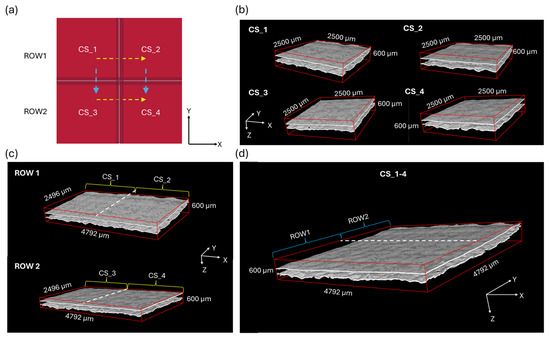
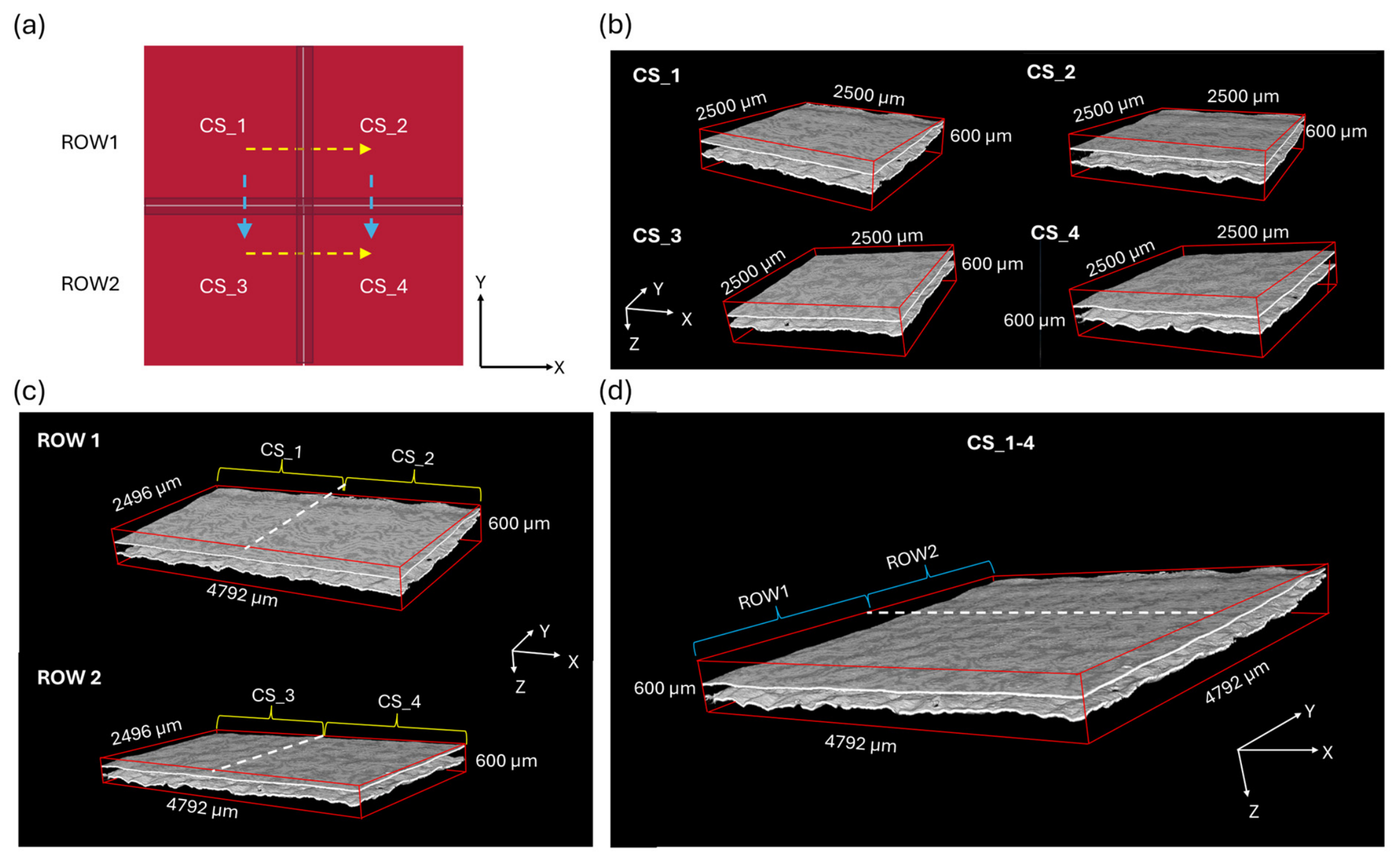
The classified stacks (each measuring 703 × 703 × 169 pixels), arranged in a 2 × 2 matrix (Figure 5a,b), were stitched in a left-to-right, top-to-bottom sequence following the stitching procedure described above. The automated interface detection and misalignment estimation yielded the following Z-shifts: +1 pixel between CS_1 and CS_2, +2 pixels between CS_3 and CS_4, and +18 pixels between Row1 and Row2. These values correspond to OCT focal depth shifts of +3.55 µm, +7.1 µm, and +63.9 µm, respectively. The estimated shifts were applied to generate Row1 and Row2 (Figure 5c), which were then combined to obtain the final mosaic (CS_1-4) (Figure 5d). The size of the final stack volume has dimensions of 1350 × 1350 × 169 pixels, corresponding to a physical size of 4792 × 4792 × 600 µm3.
Figure 5.
Stitching results for the classified image stacks of the PRM sample. (a) Schematic representation of the stitching sequence, proceeding from left to right and top to bottom. (b) Four classified image stacks obtained from the segmentation of OCT volumes. (c) Pairwise alignment and registration of the classified image stacks to generate intermediate mosaics (Row1 and Row2). (d) Final stitched image stack.
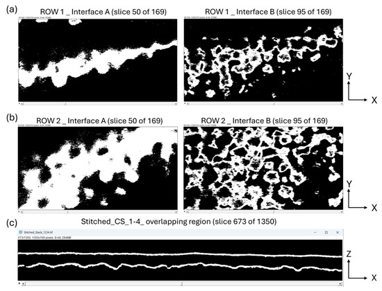
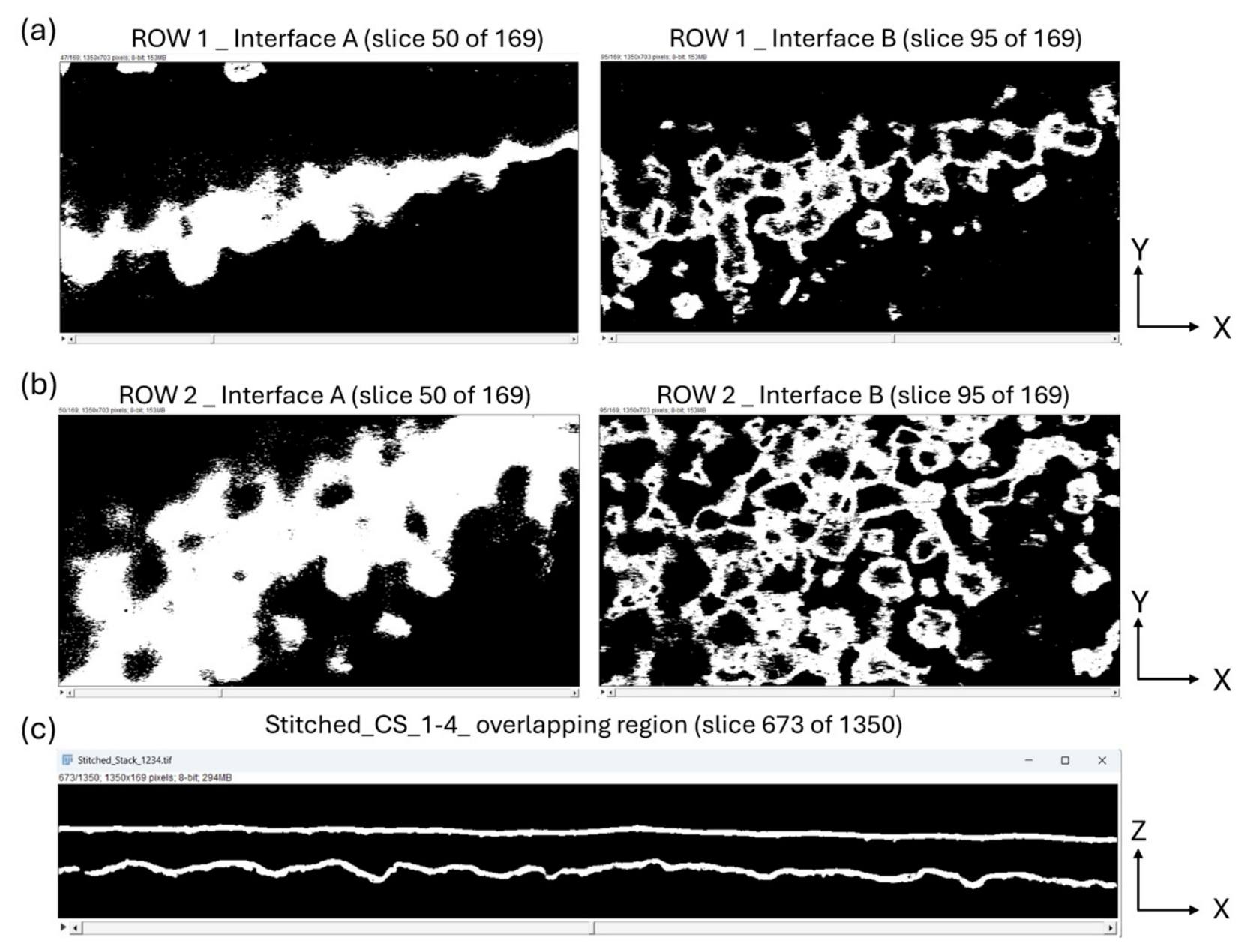
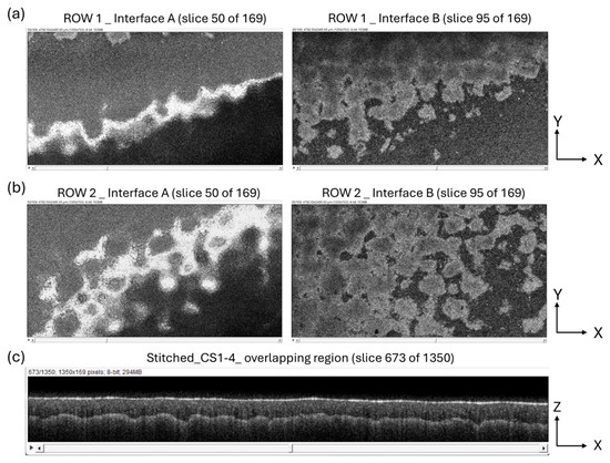
The effectiveness of the stitching procedure is illustrated in Figure 6. The image stacks Row1 (a) and Row2 (b) were resliced to provide an XY view of the overlapping region at two different axial depths, corresponding to interface A (paint/air) and interface B (paint/primer), i.e., XY slice 50 and XY slice 95, respectively. As shown, no visible discontinuities are observed between the two stacks after stitching.
Figure 6.
Demonstration of the robustness of the proposed stitching procedure for the classified stacks. XY view of stacks Row1 (a) and Row2 (b) at two different axial depths, corresponding to interface A (paint/air) and interface B (paint/primer), namely slices 50 and 95, respectively. XZ slice 673 (c) extracted from the final CS_1-4 mosaic in the overlapping region between Row1 and Row2.
Consistently, the XZ slice 673 of the final CS_1-4 mosaic (Figure 6c), located at the center of the overlapping region (B-slices 647–703) between Row1 and Row2, exhibits a smooth and well-aligned transition. These results confirm the robustness and accuracy of the proposed stitching procedure.
4.1.2. Paint Thickness Computation
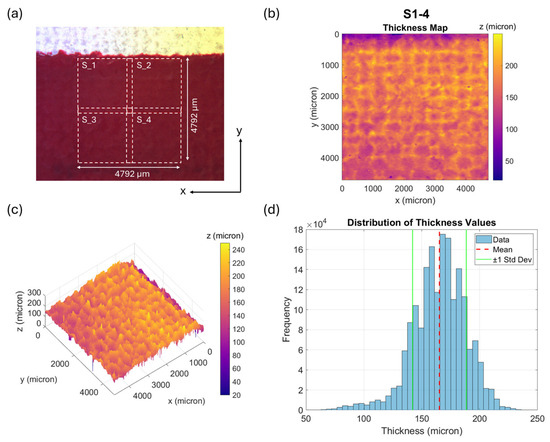
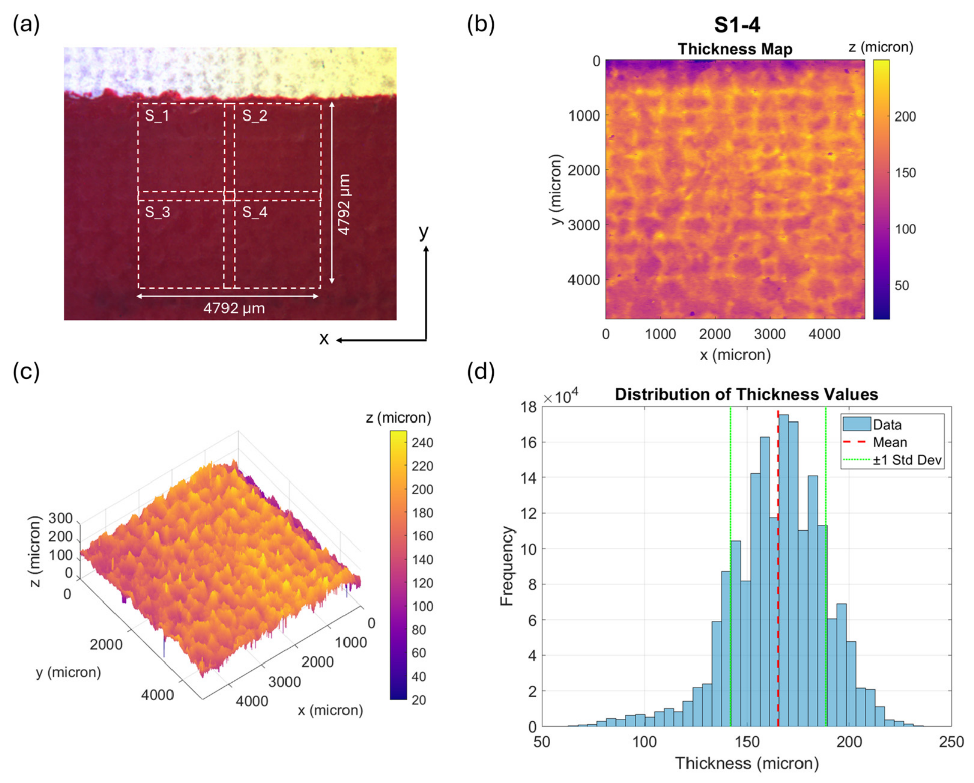
Following outliers’ removal, the final stitched binary stack was imported into MATLAB for paint layer thickness computation. The results are shown in Figure 7, displaying the acquisition areas traced on the sample’s surface (a), the corresponding pixel-by-pixel thickness map encoded on a color scale, displayed in 2D (b) and in 3D (c), and a histogram of thickness values (d). The histogram includes the mean value (red dashed line) and the standard deviation range (bounded by green lines). The analysis was also performed on the single stacks before the stitching, as reported in Figure A1 (S_1 and S_2) and Figure A2 (S_3 and S_4).
Figure 7.
Thickness analysis of the PRM paint on canvas: (a) FOV brightfield image with OCT measurement areas indicated by the dashed squares; (b) 2D and (c) 3D color-coded thickness map (XY = 4792 × 4792 µm2); (d) histogram showing the statistical distribution of all measured thickness values across the stack.
Parameters related to data quality, thickness range, statistical analysis, and derived values for all analyzed volumes (single and stitched stacks) are reported in Table 2.
Table 2.
Summary of the OCT measurement statistics for the analyzed PRM stacks.
As for the stitched S_1-4, out of a total of 1,822,500 valid pixels (1350 × 1350), the number of invalid pixels was 2747, corresponding to approximately 0.15%. The invalid pixels originate from the segmentation step rather than from the stitching procedure and correspond to local discontinuities in the detected interfaces, where isolated missing pixels prevent local thickness computation. They are mainly concentrated in low-contrast regions, where segmentation uncertainty is higher.
The color maps revealed thickness variations at high spatial resolution, further demonstrating the effectiveness of the segmentation process in resolving micro-morphological features at the two material interfaces. The mean optical thickness ± standard deviation was 167.5 ± 23.7 µm, which, after correction for the refractive index of the medium (n = 1.5), corresponds to a real geometric thickness of 111.7 ± 15.8 µm.
4.1.3. Stitching of OCT Volumes
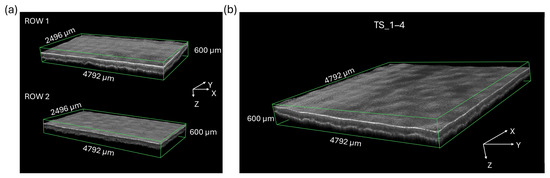
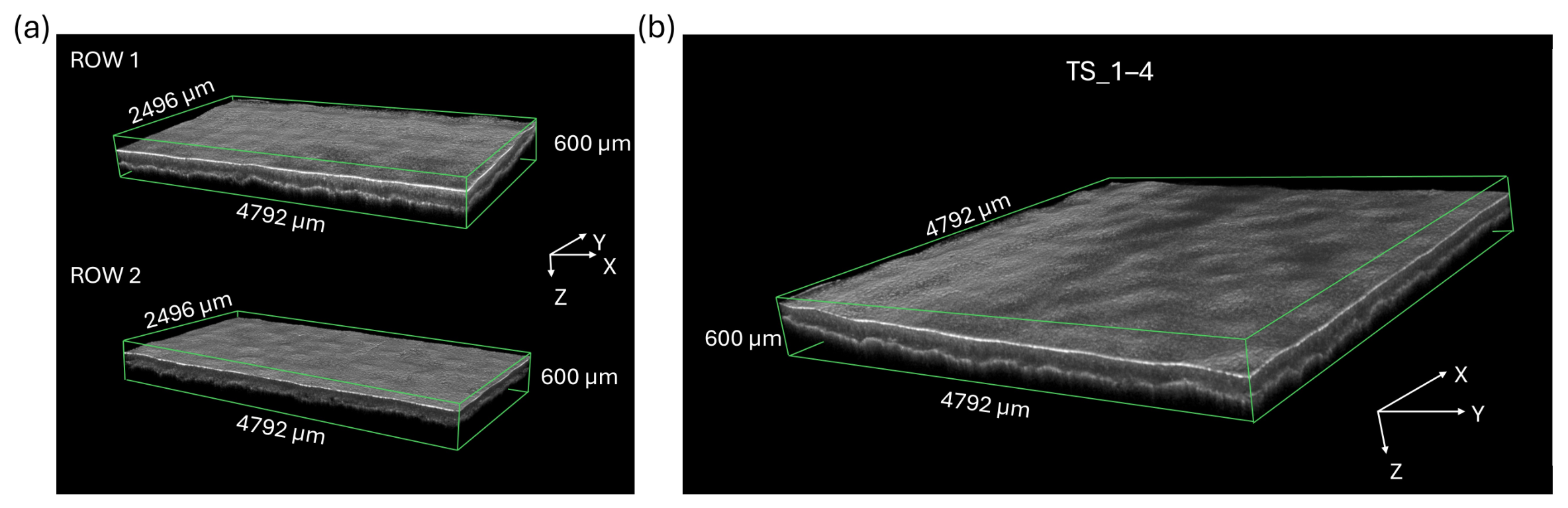
The stitching of the original OCT volumes was performed by applying the Z-shifts previously estimated through the automated interface detection. The tomographic stacks were aligned and registered pairwise along the lateral X-direction, as described above, to generate Row1 and Row2 (Figure 8a), which were subsequently stitched along the Y-direction using the same cosine-weighted blending approach within the 56-pixel overlapping region, resulting in a smoothly assembled final OCT volume (Figure 8b).
Figure 8.
Stitching results for the tomographic image stacks of the PRM sample. (a) Pairwise alignment and registration of TS_1-2 and TS_3-4 to generate intermediate mosaics (Row1 and Row2). (b) Final OCT volume (TS_1-4).
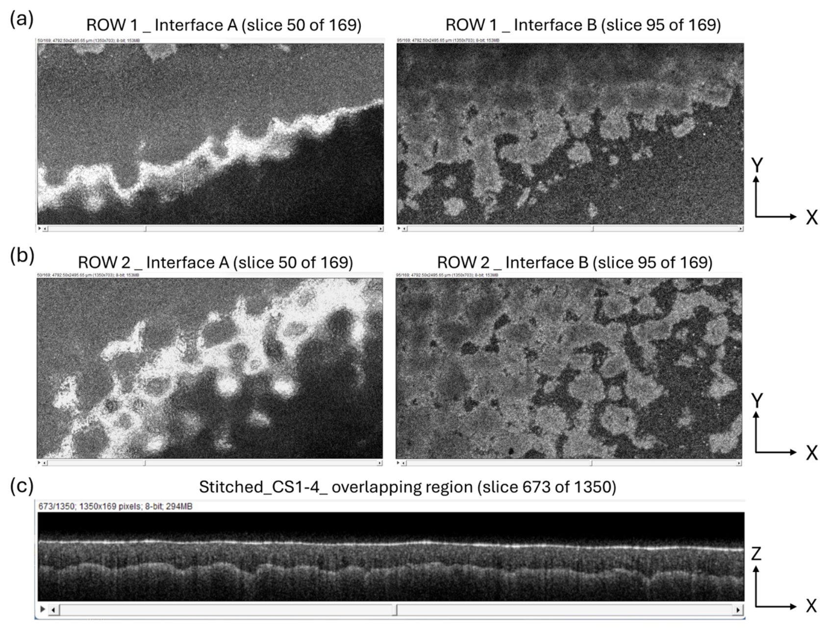
Similar to Figure 6 for the classified image stacks, the effectiveness of the stitching procedure is illustrated in Figure 9 for the tomographic stacks. The XY slices of Row1 (a) and Row2 (b) provide a view of interface A (paint/air, slice 50) and interface B (paint/primer, slice 95). No visible discontinuities are observed in the overlapping region between the two stacks after stitching. Consistently, the XZ slice 673 of the final TS_1-4 mosaic (Figure 9c), located at the center of the overlapping region between Row1 and Row2, exhibits a smooth and well-aligned transition.
Figure 9.
Demonstration of the robustness of the proposed stitching procedure for the tomographic volumes. XY view of stacks Row1 (a) and Row2 (b) at two different axial depths, corresponding to interface A (paint/air) and interface B (paint/primer), namely slices 50 and 95, respectively. XZ slice 673 (c) extracted from the final CS_1-4 mosaic, located at the center of the overlapping region between Row1 and Row2.
An additional slice-based visualization of the final mosaic (Figure A3) further demonstrates the accuracy and robustness of the proposed methodology. In particular, XY slices 50 and 68 enable the visualization of interface A, whereas slices 95 and 113 correspond to the axial depth of interface B. Slices 68 and 113 correspond to slices 50 and 95 in Row 2 of Figure 9b, respectively, after applying the estimated axial displacement (Z-shift of +18 pixels) required for image alignment.
Finally, we performed an ablation analysis of the pipeline components. The stitching procedure was repeated while excluding two key processing steps, namely the estimation of the Z-shifts and the cosine-weighted blending within the overlapping regions (Figure A4, Figure A5 and Figure A6). As a result, both the classified mosaics (Figure A4a,c) and the tomographic mosaics (Figure A4b,d) exhibit evident misalignments along the X, Y, and Z directions. These artifacts are further emphasized in the XY and XZ slices extracted from CS_1-4 (Figure A5) and TS_1-4 (Figure A6). This clearly highlights the fundamental role of the proposed alignment and blending strategy in ensuring the geometric consistency and visual continuity of the reconstructed mosaic.
4.2. Lemon Yellow (LY) on Primed Wooden Panel
4.2.1. Classified Image Stitching
For the segmentation of the LY sample, the RF classifier was independently trained on two acquisition groups (CS1_1-4 and CS2_1-4), each comprising four image stacks, resulting in two separate models. Separate training was required due to differences in morphological characteristics, including variations in layer thickness and interface signal intensity. The two models were then applied to the corresponding unseen test datasets (CS3_1-4 and CS4_1-4), and their performance was evaluated. A total of 285,085 and 294,748 annotated pixels were used for training the two models, respectively, corresponding to approximately the area of three full B-scans. Considering the combined size of the four stacks (each consisting of 703 B-scans of 703 × 140 pixels, for a total of approximately 69.2 million pixels), the annotated samples represent about 0.99% of the entire dataset.
The first model achieved strong overall performance (Table 3), with 275,402 correctly classified instances out of 285,085, corresponding to an accuracy of 96.6%. The confusion matrix indicates a reliable separation between the two classes, with F1-scores of 0.931 for class 1 and 0.978 for class 2, and a weighted average F1-score of 0.966. The corresponding IoU values are 0.870 for class 1 and 0.956 for class 2, resulting in a weighted average IoU of 0.935. The MCC value of 0.908 confirms a strong agreement between predictions and ground truth, while the ROC area (0.993) highlights the excellent discriminative capability of the model.
Table 3.
Classifier’s performance metrics for the segmentation of LY stacks CS1_1-4 and CS3_1-4.
The second model also shows high classification performance (Table 4), with 284,238 correctly classified instances out of 294,748, corresponding to an accuracy of 96.4%. The misclassification rate is 3.6%, indicating stable predictive behavior. Class-wise results yield F1-scores of 0.928 for class 1 and 0.976 for class 2, with a weighted average F1-score of 0.964. The corresponding IoU values are 0.865 for class 1 and 0.954 for class 2, resulting in a weighted average IoU of 0.931. The MCC value of 0.904 confirms a strong correlation between predicted and reference labels, while the ROC area (0.993) further demonstrates the robustness and discriminative power of the model across both classes.
Table 4.
Classifier’s performance metrics for the segmentation of LY stacks CS2_1-4 and CS4_1-4.
The two trained models were used for the segmentation of the sixteen tomographic stacks (Figure A7), yielding the respective classified stacks (Figure A8).
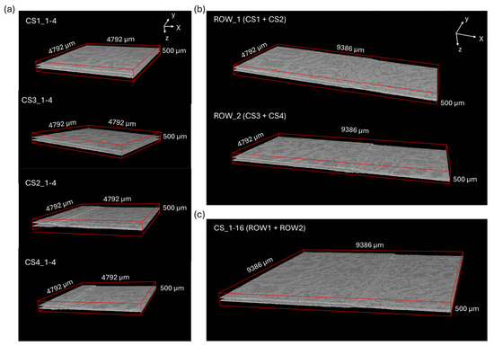
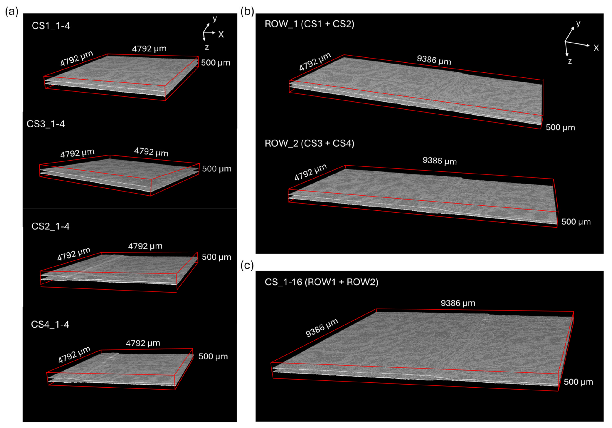
The four groups of classified stacks (each measuring 2496 × 2496 × 500 µm3), arranged in 2 × 2 matrices, were stitched in a left-to-right, top-to-bottom sequence following the procedure previously described, resulting in the four mosaics (4792 × 4792 × 500 µm3) reported in Figure 10a. Then, intermediate stacks Row1 and Row2 (Figure 10b) were generated and subsequently combined to obtain the final mosaic (CS_1-16), for a total size of 9386 × 9386 × 500 µm3 (Figure 10c). The estimated Z-shifts for each 2 × 2 mosaic and the final stack are reported with the corresponding OCT focal depth shifts in Table 5.
Figure 10.
Stitching results for the classified image stacks of the LY sample. (a) Four classified image stacks obtained from the pairwise alignment and registration of the 16 classified image stacks arranged in 2 × 2 matrices. (b) Row1 and Row2 generated from the stitching of CS1–CS2 and CS3–CS4. (c) Final stitched image stack (CS_1-16).
Table 5.
Estimated Z-shifts (in pixels) and corresponding OCT focal depth shifts (in µm) for LY stacks.
4.2.2. Paint Thickness Computation
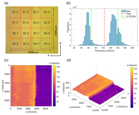
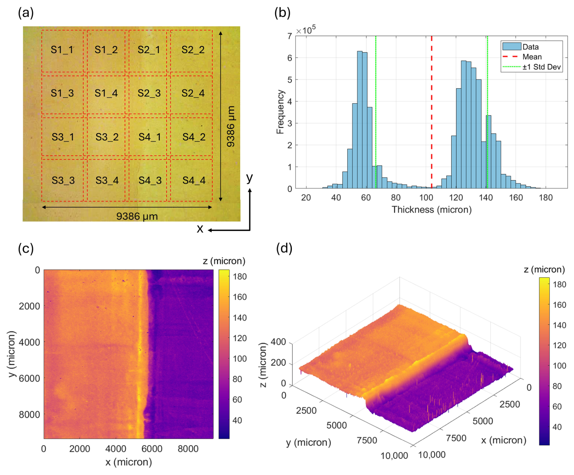
The final stitched binary stack was analyzed for paint layer thickness quantification. The results are shown in Figure 11, which reports the acquisition regions traced on the sample surface (a), the pixel-wise thickness map displayed in 2D (c) and 3D (d), and the corresponding thickness histogram (b).
Figure 11.
Thickness analysis of the LY paint on the wooden panel: (a) FOV brightfield image with OCT measurement areas indicated by the dashed squares; (b) histogram showing the statistical distribution of all measured thickness values across the stack; (c) 2D and (d) 3D color-coded thickness map (XY = 9386 × 9386 µm3).
The thickness maps reveal well-resolved spatial variations at high resolution and enable clear discrimination between the two paint thicknesses. In particular, the method accurately resolves low thickness values in the region corresponding to the thinner paint layer, as well as higher values associated with the thicker layer, with a well-defined thickness step at their boundary. This confirms the capability of the proposed approach to quantitatively reconstruct spatially varying coating thicknesses.
Table 6 summarizes the statistical descriptors and derived thickness parameters for the intermediate stitched datasets (S1_1-4 to S4_1-4) and for the final mosaic (S1-4). Among the intermediate results, S1_1-4 and S3_1-4 exhibit lower dispersion, while S2_1-4 and S4_1-4 show higher variability, reflecting local heterogeneity within the analyzed regions. The final S_1-16 dataset provides the most comprehensive representation of the sample, integrating both thickness regimes over 6,990,736 valid measurements with 68,101 bad indexes, corresponding to 0.97% of the total measurements. It yields a mean optical thickness of 103.8 µm with a standard deviation of 23.7 µm, while the derived mean geometric thickness of 69.2 µm reflects the combined contribution of the thin and thick paint layers across the reconstructed surface.
Table 6.
Summary of the OCT measurement statistics for the analyzed LY stacks.
The mean thickness of the two paint layers was additionally evaluated over a 3 × 8 mm2 region to estimate the bias with respect to the Kapton tape used as a reference for layer deposition, which may be affected by manual sample preparation. Further details are provided in Appendix A (Figure A10).
4.2.3. Stitching of OCT Volumes
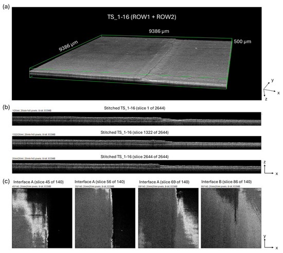
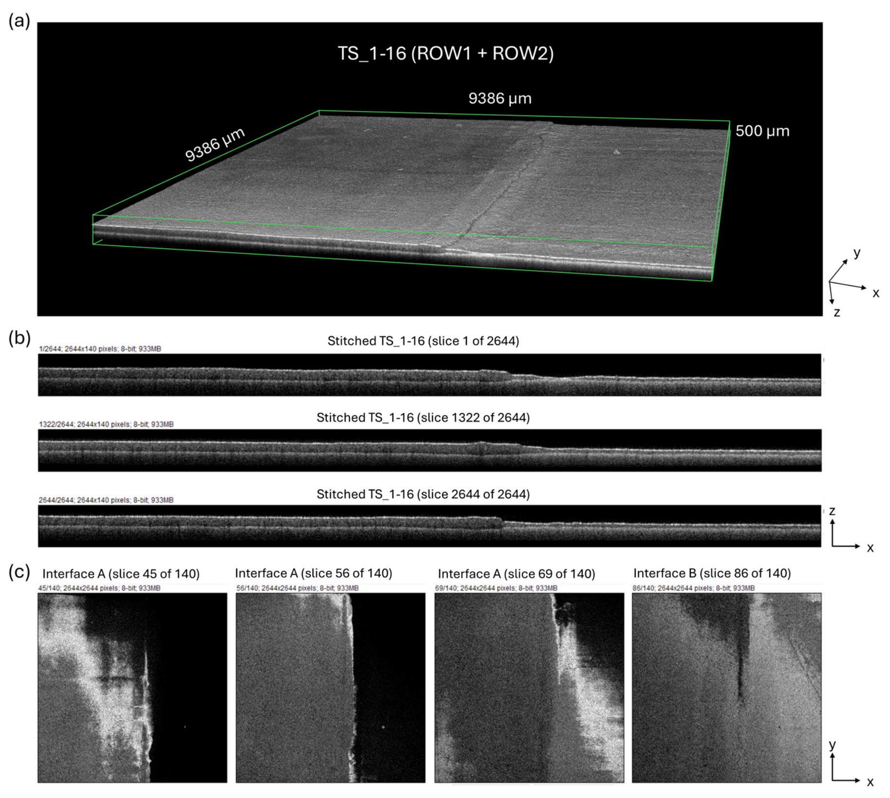
The stitching result obtained for the original OCT volumes is presented in Figure 12. The previously estimated Z-shifts were applied to generate Row1 and Row2, which were subsequently merged along the Y-direction using a cosine-weighted blending strategy within the 56-pixel overlap region, yielding the final reconstructed OCT volume shown in Figure 12a.
Figure 12.
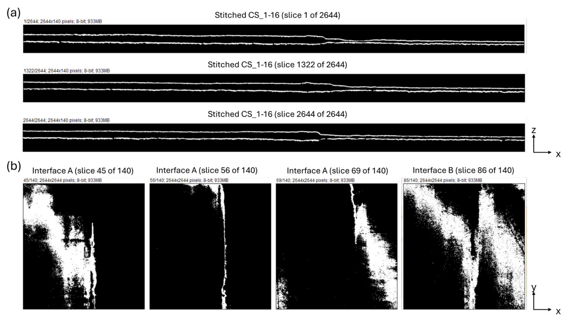
Result of tomographic stitching for the LY sample: (a) final reconstructed OCT volume, TS1-16; (b) XZ cross-sections extracted from the final mosaic; (c) XY views showing interface A (paint/air) and interface B (paint/primer).
The performance of the stitching procedure was further evaluated through representative XZ cross-sections extracted from the final TS1-16 mosaic (Figure 12b). In particular, slices acquired at the beginning of the stack (slice 1), at the center of the overlap region between Row1 and Row2 (slice 1322), and at the end of the stack (slice 2644) were analyzed. No visible discontinuities or misalignments were observed at the transitions between adjacent stitched volumes, confirming the geometric consistency of the reconstruction.
Additional validation was provided by the XY views reported in Figure 12c, which illustrate interface A (paint/air) and interface B (paint/primer). Specifically, slices 45 and 56 highlight the surface morphology of the thicker paint layer, slice 69 corresponds to the thinner paint layer, and slice 86 shows the primer layer surface. In all cases examined, the interfaces exhibit smooth and continuous transitions across the stitched regions, further demonstrating the effectiveness of the proposed stitching approach.
For completeness, the corresponding XY and XZ views obtained from the final classified stack CS1-16 are reported in Figure A9, where the continuity of the transitions at interfaces A and B can also be observed.
5. Discussion
The proposed methodology consists of sequential steps that are performed in an integrated supervised ML-based computational framework to provide large-scale stratigraphic analysis of painting layers.
The adopted segmentation strategy, in which the two interfaces were grouped into a single class, proved effective despite the different optical properties of the investigated materials. In particular, the OCT signal intensity was higher at the paint/air interface than at the paint/primer interface because of differences in reflectivity and optical transparency to the probing radiation. Moreover, the higher percentage of invalid thickness measurements recorded for the LY sample (0.97%) compared with the PRM sample (0.15%) can be ascribed to the greater scattering exhibited by the LY paint layer, which tends to enhance signal attenuation and degrade interface contrast.
Another potential source of misclassification, especially for the PRM sample, was related to the different morphology of the paint and primer layers. While the paint surface appeared relatively flat, the primer layer showed a more pronounced waviness due to the underlying canvas fibers. Nevertheless, these differences did not significantly affect the segmentation performance, confirming the robustness of the proposed approach. A key requirement for the successful application of the workflow is the quality (i.e., representativeness) of the annotations, which are inherently operator-dependent, as is typical for manually annotated training datasets.
The potential risk of overfitting was evaluated through the adopted 10-fold cross-validation scheme. This approach affords internal validation of model performance, as each subset is held out in turn and tested independently. The cross-fold consistency of the results indicates stable model behavior and substantiates the generalization capability of the proposed method, with no indication of overfitting emerging under the present experimental conditions.
An additional advantage of the proposed workflow is the progressive reduction in data size throughout the different processing stages, which significantly improves data handling and computational efficiency. The original OCT tomographic volume acquired in proprietary format (703 × 703 × 140 pixels, corresponding to a physical volume of 2.5 × 2.5 × 0.5 mm with a voxel size of 3.55 µm3) required approximately 6.11 GB of storage. Following conversion into a TIFF image stack using the Thorlabs software (version 5.7.2.0), the data size decreased to 264 MB due to the extraction of the volumetric information into individual RGB image slices. A further reduction was obtained by converting the image stack into 8-bit grayscale format, resulting in a final size of 66 MB for each tomographic stack.
The segmentation step provided further optimization of the data volume. Each classified stack, preserving the original spatial dimensions (703 × 703 × 140 pixels), occupied approximately 61.1 MB. After the stitching procedure, the final 2 × 2 mosaic of classified stacks (2644 × 2644 × 140 pixels) required only 26.2 MB, whereas the corresponding stitched tomographic mosaic in 8-bit format occupied 566 MB.
These results demonstrate that the proposed processing chain enables accurate volumetric reconstruction and classification with robust performance while also substantially reducing storage requirements, thereby facilitating the management, visualization, and analysis of large-scale OCT datasets.
Although this workflow was validated on two representative paint samples, it is readily extendable to more complex and heterogeneous stratified objects. Its applicability is primarily constrained by physical factors inherent to OCT imaging, including the optical penetration depth of the probing radiation and the interplay between layer thickness, axial resolution, and imaging depth. Provided that these conditions are met, the approach can be transferred to other material systems irrespective of their specific composition or scattering behavior. In such instances, however, newly annotated training data would be necessary to guarantee reliable interface detection. The extension of the method to these contexts will constitute the subject of future investigations, aimed at enhancing its suitability for real-case scenarios.
6. Conclusions
We have presented a new workflow for OCT post-processing to extend stratigraphic characterization of paintings to macroscopic fields of view. The approach allows for (i) supervised semantic segmentation applied to OCT image stacks to identify material layer interfaces; (ii) seamless registration and stitching of image stacks via interface-based alignment and blending; and (iii) automated pixel-wise computation of paint layer thickness.
The user-friendly workflow does not require advanced programming expertise, since the segmentation is performed with a customizable and freely available plugin integrated into Fiji, which enables the use of ImageJ image processing tools, while the classifier’s performance can be thoroughly evaluated using standard quantitative metrics. The proposed method enables automated and reproducible pixel-by-pixel analysis of OCT 3D data, achieving performance levels unattainable with traditional manual analysis. The model discriminates air/paint and paint/primer interfaces with 96.4–97.1% accuracy and a weighted average F1-score > 0.95. The resulting thickness maps enable quantitative coating thickness mapping with micrometric resolution, and the reconstructed OCT volumes exhibit seamless stitched transitions.
The approach can be extended to image stacks generated by other stratigraphic techniques operating at different scales, such as Non-Linear Optical Microscopy (NLOM), terahertz imaging, and computed tomography.
To the best of our knowledge, this work represents the first application of an AI-based, fully automated stitching and thickness quantification framework to OCT data in the field of cultural heritage. This contribution enhances the accessibility of AI-based technologies to a broader range of heritage science professionals while retaining expert supervision throughout the workflow.
Author Contributions
Conceptualization, A.D.F. and R.F.; methodology, A.D.F.; validation, A.D.F.; formal analysis, A.D.F.; investigation, A.D.F.; resources, A.D.F.; data curation, A.D.F.; software, A.D.F.; writing—original draft preparation, A.D.F.; writing—review and editing, A.D.F. and R.F. All authors have read and agreed to the published version of the manuscript.
Funding
This research received no external funding.
Data Availability Statement
The raw data supporting the conclusions of this article will be made available by the authors on request.
Conflicts of Interest
The authors declare no conflicts of interest.
Abbreviations
The following abbreviations are used in this manuscript:
| AUC | Area Under The Curve |
| CNNs | Convolutional Neural Networks |
| CS | Cultural Heritage |
| DL | Deep Learning |
| EFL | Effective Focal Length |
| FTL | Fast Fourier Transform |
| FOV | Field Of View |
| FCNs | Fully Convolutional Neural Networks |
| IoU | Intersection Over Union |
| ML | Machine Learning |
| MCC | Matthews Correlation Coefficient |
| NIR | Near Infrared |
| OCT | Optical Coherence Tomography |
| PRM | Primary Red Magenta |
| ROC | Receiver Operating Characteristic |
| RNNs | Recurrent Neural Networks |
| SD-OCT | Spectral-Domain Optical Coherence Tomography |
| SLD | Super Luminescent Diode |
| TWS | Trainable Weka Segmentation |
Appendix A
Figure A1.
Thickness analysis of the PRM paint on canvas for stacks S_1 (a,c) and S_2 (b,d): 2D color-coded thickness map (XY = 2496 × 2496 µm2) and histograms showing the statistical distribution of all measured thickness values across each stack.
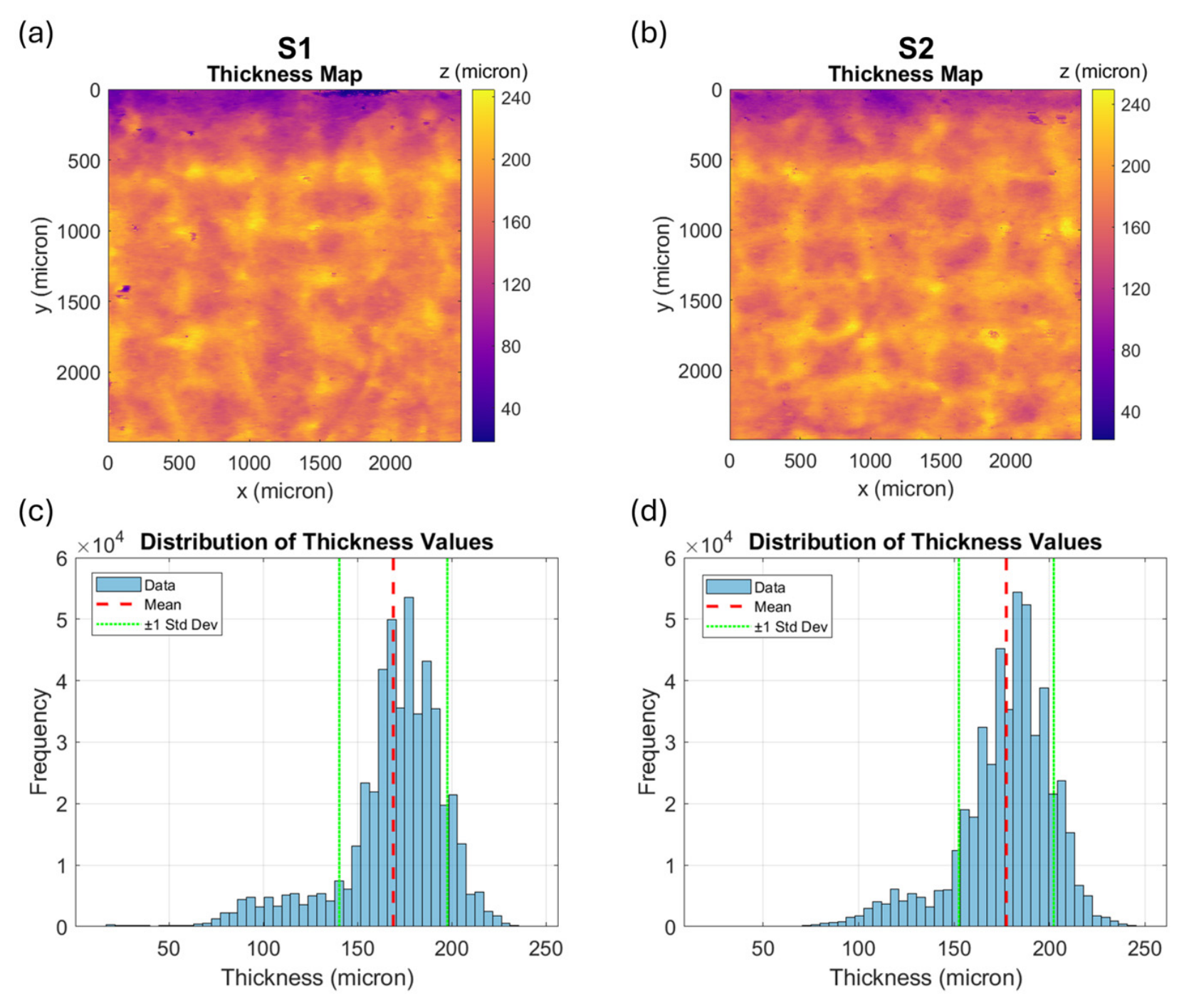
Figure A2.
Thickness analysis of the PRM paint on canvas for stacks S_3 (a,c) and S_4 (b,d): 2D color-coded thickness map (XY = 2496 × 2496 µm2) and histograms showing the statistical distribution of all measured thickness values across each stack.
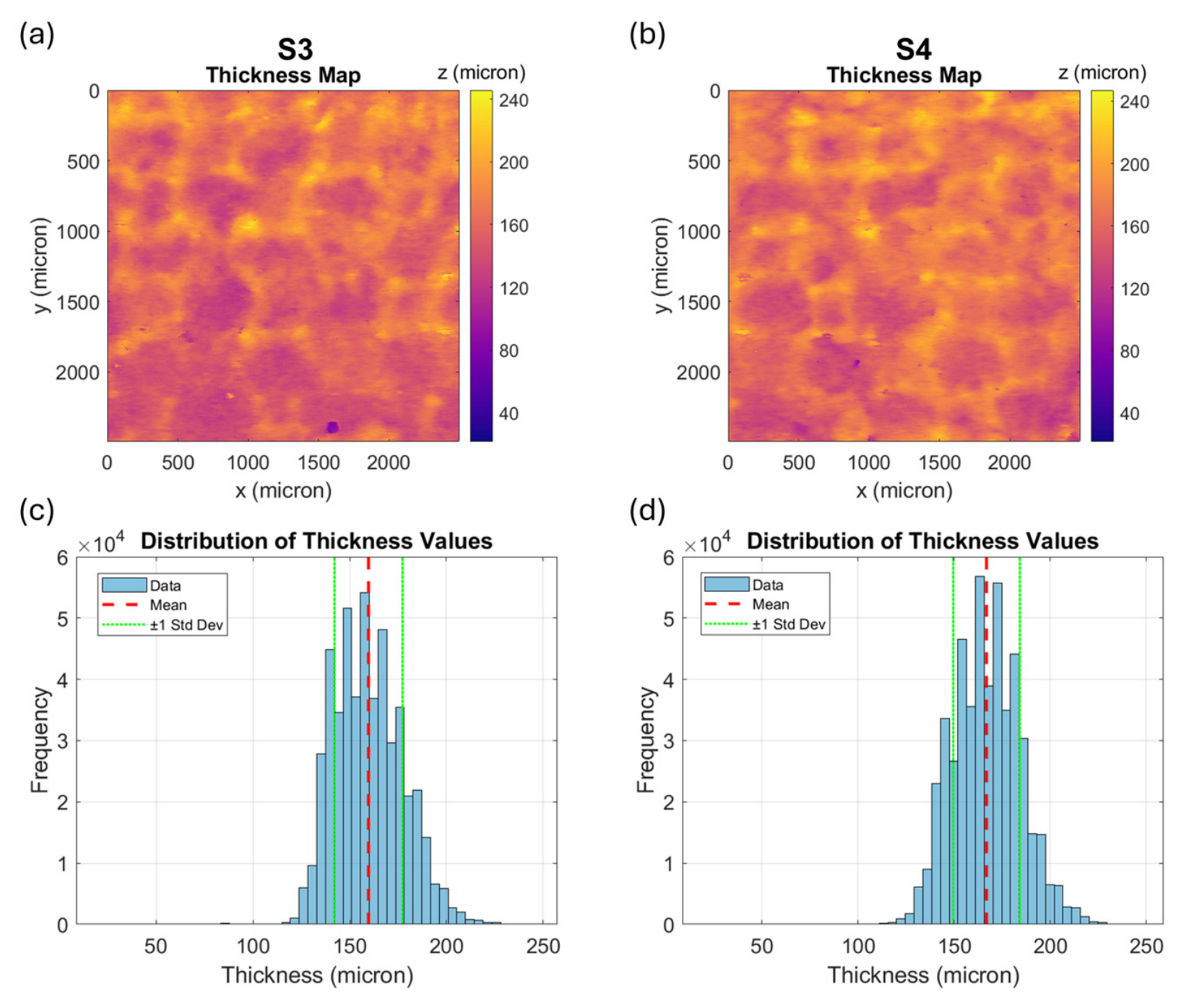
Figure A3.
XY views of the stitched tomographic volume (TS_1–4) for the PRM sample. XY slices 50 and 68 enable the visualization of paint/air interface A (a,c), whereas slices 95 and 113 correspond to the axial depth of paint/primer interface B (b,d).
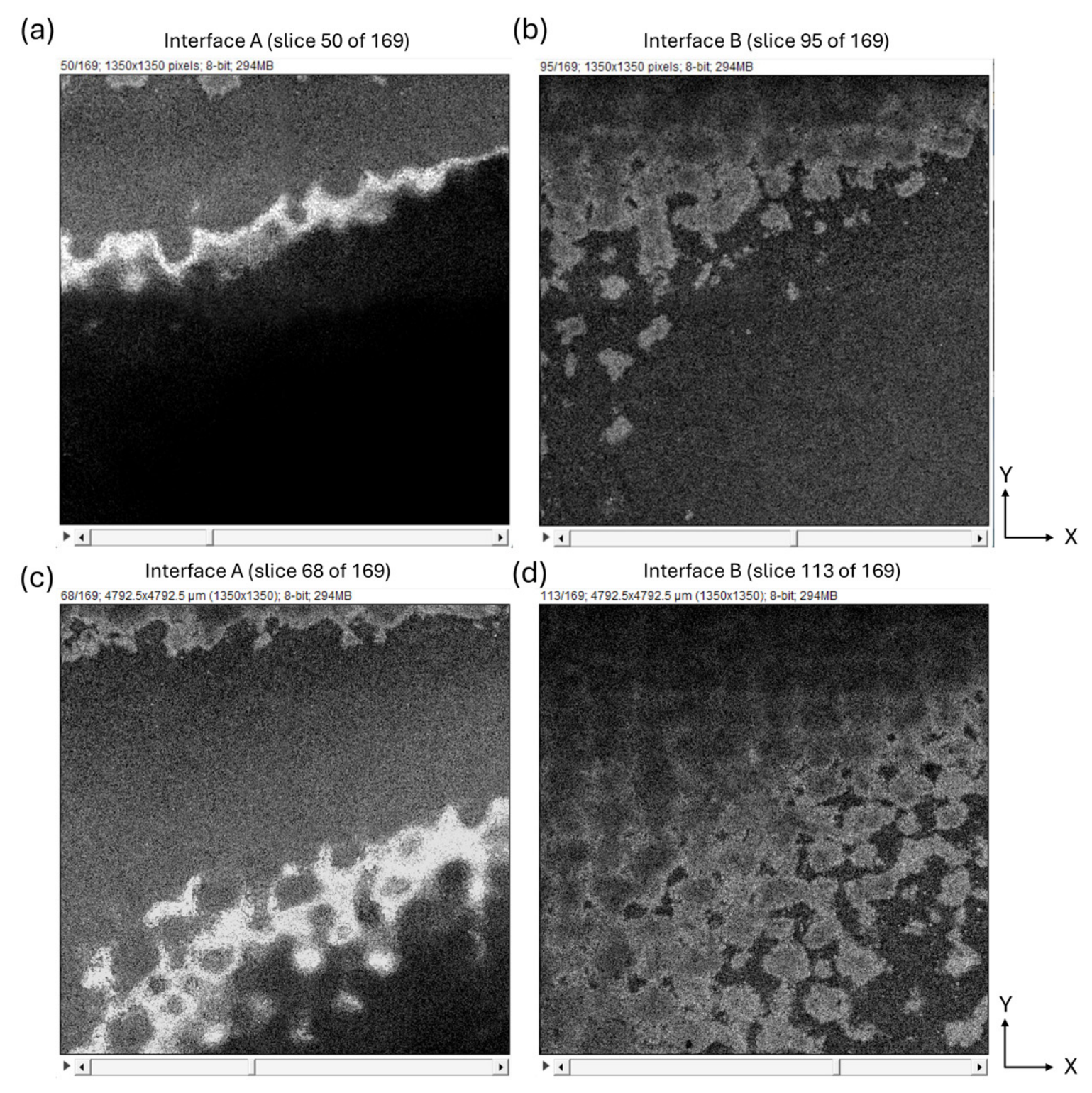
Figure A4.
Results of the stitching procedure performed without Z-shift estimation and blending within the overlapping regions. The 3D renderings of both the classified mosaics (a,c) and the tomographic mosaics (b,d) exhibit evident misalignments along the X, Y, and Z directions.
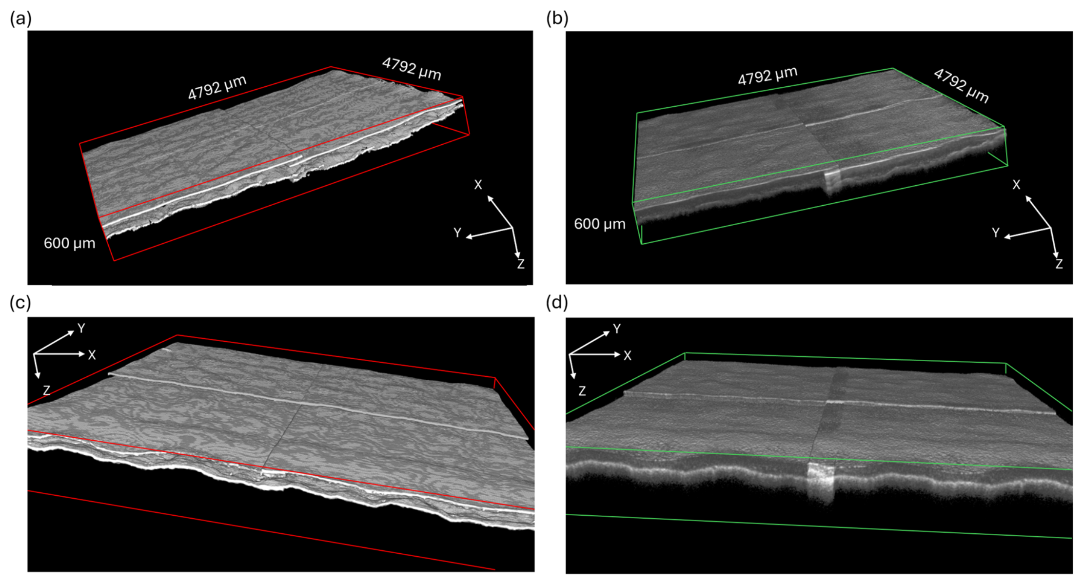
Figure A5.
Results of the stitching procedure performed without Z-shift estimation and blending within the overlapping regions. XY views of the stitched classified stack CS_1-4 at two different axial depths, slice 50 (a) and slice 95 (b), corresponding to interface A (paint/air) and interface B (paint/primer). XZ slice 673 (c), located at the center of the overlapping region between Row1 and Row2.
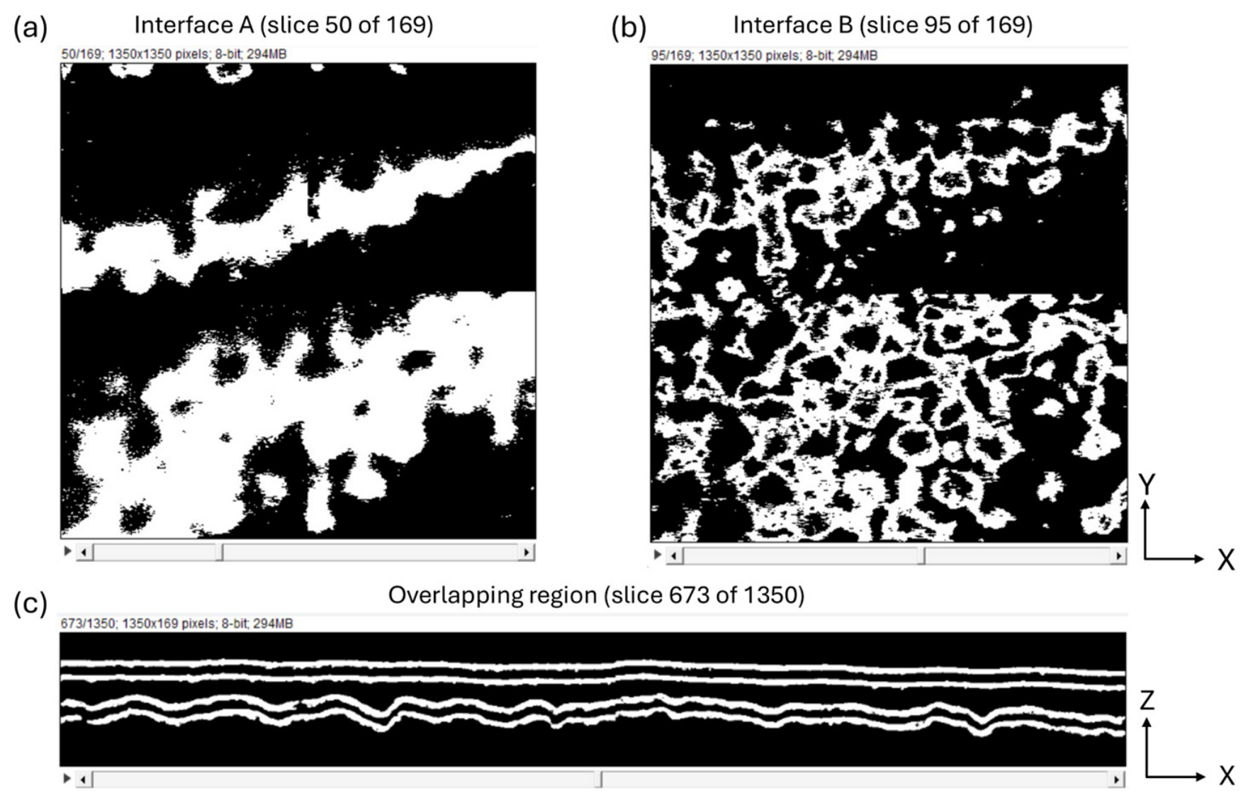
Figure A6.
Results of the stitching procedure performed without Z-shift estimation and blending within the overlapping regions. XY views of the stitched tomographic volume TS_1-4 at two different axial depths, slice 50 (a) and slice 95 (b), corresponding to interface A (paint/air) and interface B (paint/primer). XZ slice 673 (c), located at the center of the overlapping region between Row1 and Row2.
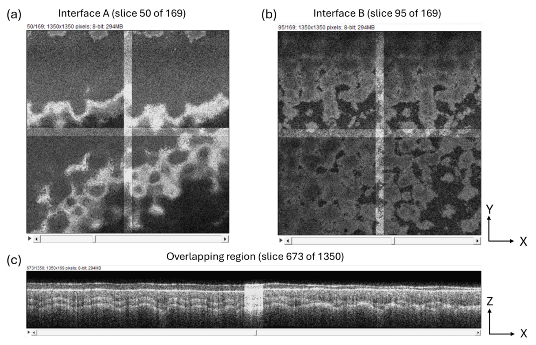
Figure A7.
The sixteen tomographic volumes acquired on the LY sample: four volumes for TS1 (a), TS2 (b), TS3 (c), and TS4 (d), respectively.
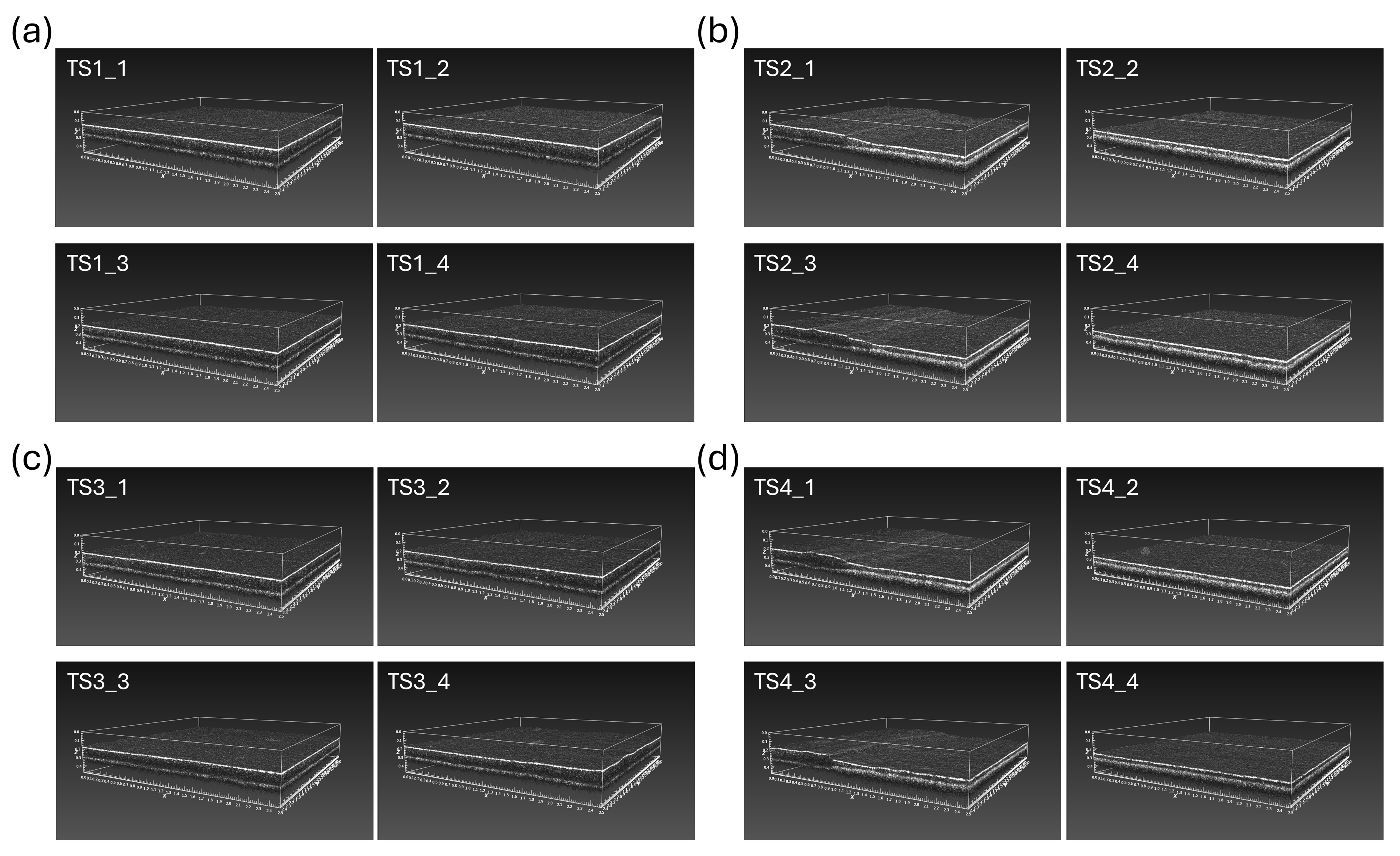
Figure A8.
The sixteen classified image stacks resulting from the segmentation of the LY tomographic volumes: four stacks for CS1 (a), CS2 (b), CS3 (c), and CS4 (d), respectively.
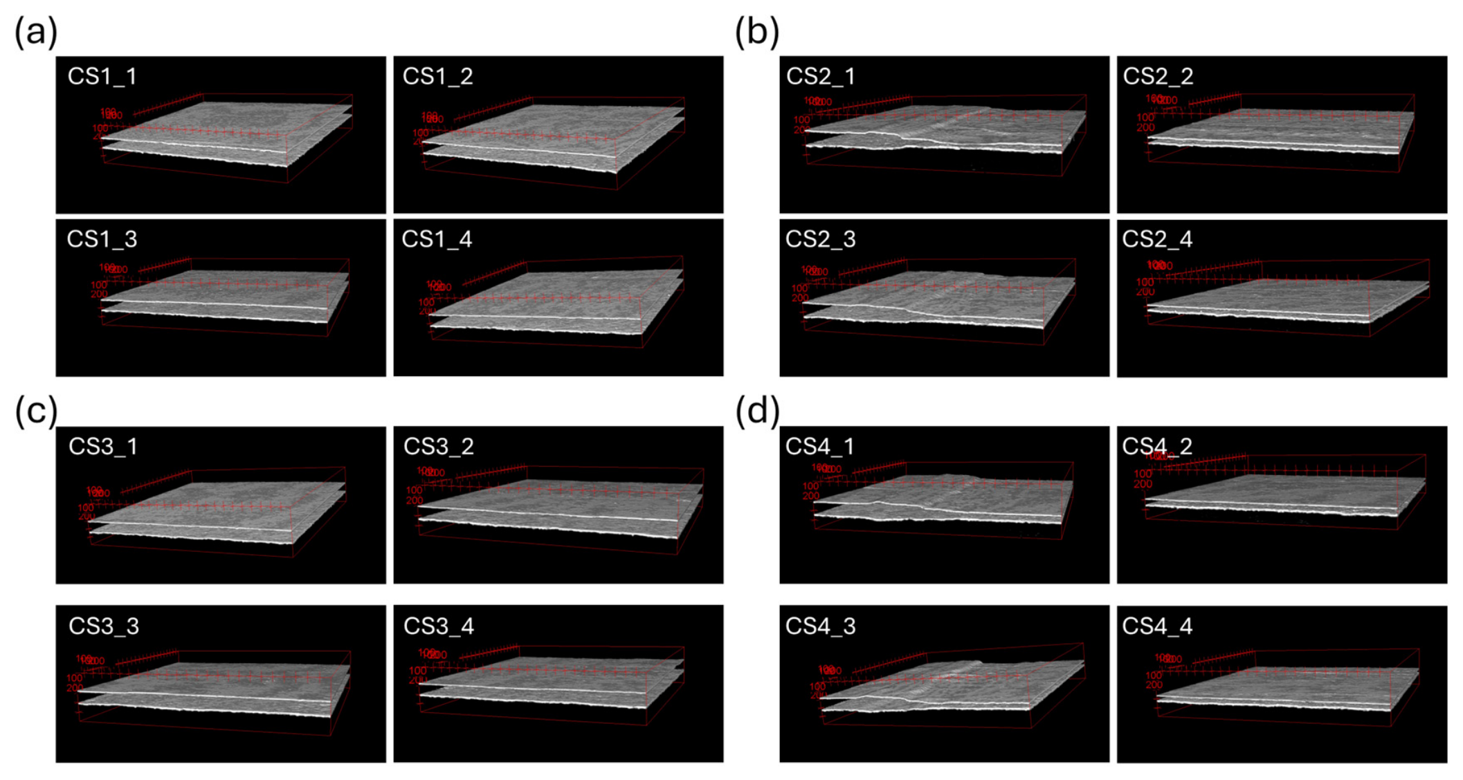
Figure A9.
Stitching results for the LY classified stacks: XZ cross-sections (a) and XY views (b) of the final mosaic, showing smooth transitions and no visible discontinuities between adjacent stacks at interface A (paint/air) and interface B (paint/primer).
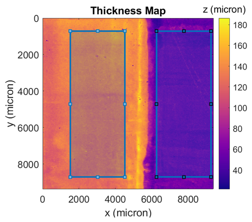
To obtain an estimate of the thickness bias and standard deviation of the LY sample with the Kapton tape reference, we evaluated the mean thickness and standard deviation over homogeneous 3 × 8 mm2 regions of the final LY thickness map (Figure A10), excluding the transition area between the two thickness steps, obtaining 37.6 ± 3.5 µm and 86.6 ± 5.3 µm from the nominal 50 ± 5 µm and 100 ± 10 µm Kapton thickness, respectively. These regions are representative of the analyzed portion of the sample but not of the entire paint layers, since only a limited area was measured with OCT (see Figure 1). This local bias may be attributed to the shrinkage of the paint material during drying and to inhomogeneities in the coating layer near the thickness transition during sample preparation. This discrepancy does not affect the validity of the proposed method.
Figure A10.
Color-coded thickness map of the LY sample, showing two rectangular regions of interest (3 × 8 mm2) used for the estimation of mean thickness and standard deviation.
References
- Targowski, P.; Iwanicka, M. Optical Coherence Tomography: Its Role in the Non-Invasive Structural Examination and Conservation of Cultural Heritage Objects—A Review. Appl. Phys. A 2012, 106, 265–277. [Google Scholar] [CrossRef] [Scilit]
- Targowski, P.; Kowalska, M.; Sylwestrzak, M.; Iwanicka, M. OCT for Examination of Cultural Heritage Objects. In Optical Coherence Tomography and Its Non-Medical Applications; Wang, M.R., Ed.; IntechOpen: London, UK, 2020. [Google Scholar]
- Liang, H.; Cid, M.G.; Cucu, R.G.; Dobre, G.M.; Podoleanu, A.G.; Pedro, J.; Saunders, D. En-Face Optical Coherence Tomography—A Novel Application of Non-Invasive Imaging to Art Conservation. Opt. Express 2005, 13, 6133–6144. [Google Scholar] [CrossRef] [Scilit] [PubMed]
- Preibisch, S.; Saalfeld, S.; Tomancak, P. Globally Optimal Stitching of Tiled 3D Microscopic Image Acquisitions. Bioinformatics 2009, 25, 1463–1465. [Google Scholar] [CrossRef] [Scilit] [PubMed]
- Murtin, C.; Frindel, C.; Rousseau, D.; Ito, K. Image Processing for Precise Three-Dimensional Registration and Stitching of Thick High-Resolution Laser-Scanning Microscopy Image Stacks. Comput. Biol. Med. 2018, 92, 22–41. [Google Scholar] [CrossRef] [Scilit] [PubMed]
- EL Abbadi, N.K.; Al Hassani, S.A.; Abdulkhaleq, A.H. A Review over Panoramic Image Stitching Techniques. J. Phys. Conf. Ser. 2021, 1999, 012115. [Google Scholar] [CrossRef] [Scilit]
- Rankov, V.; Locke, R.J.; Edens, R.J.; Barber, P.R.; Vojnovic, B. An Algorithm for Image Stitching and Blending. In Proceedings of the Proc. SPIE 5701, Three-Dimensional and Multidimensional Microscopy: Image Acquisition and Processing XII, San Jose, CA, USA, 22–27 January 2005; p. 190. [Google Scholar]
- Ma, B.; Zimmermann, T.; Rohde, M.; Winkelbach, S.; HeFeng, F.Q.; Lindenmaier, W.; Dittmar, K.E.J. Use of Autostitch for Automatic Stitching of Microscope Images. Micron 2007, 38, 492–499. [Google Scholar] [CrossRef] [Scilit] [PubMed]
- Muhlich, J.L.; Chen, Y.-A.; Yapp, C.; Russell, D.; Santagata, S.; Sorger, P.K. Stitching and Registering Highly Multiplexed Whole-Slide Images of Tissues and Tumors Using ASHLAR. Bioinformatics 2022, 38, 4613–4621. [Google Scholar] [CrossRef] [Scilit] [PubMed]
- Jiang, G.; Wang, M.R.; Shen, K.; Baig, S.A. Wide Field-of-View High Lateral Resolution Optical Coherence Tomography with 3D Image Stitching and Superresolution. In Proceedings of the Optical Coherence Tomography and Coherence Domain Optical Methods in Biomedicine XXII, San Francisco, CA, USA, 27 January–1 February 2018; Izatt, J.A., Fujimoto, J.G., Tuchin, V.V., Eds.; SPIE: Bellingham, WA, USA, 2018; p. 99. [Google Scholar]
- Zhou, X.; In, D.; Chen, X.; McCune Bruhn, H.; Liu, X.; Yang, Y. Spectral 3D Reconstruction of Impressionist Oil Paintings Based on Macroscopic OCT Imaging. Appl. Opt. 2020, 59, 4733–4738. [Google Scholar] [CrossRef] [Scilit] [PubMed]
- Callewaert, T.; Guo, J.; Harteveld, G.; Vandivere, A.; Eisemann, E.; Dik, J.; Kalkman, J. Multi-Scale Optical Coherence Tomography Imaging and Visualization of Vermeer’s Girl with a Pearl Earring. Opt. Express 2020, 28, 26239–26256. [Google Scholar] [CrossRef] [Scilit] [PubMed]
- Callewaert, T.; Dik, J.; Kalkman, J. Segmentation of Thin Corrugated Layers in High-Resolution OCT Images. Opt. Express 2017, 25, 32816–32828. [Google Scholar] [CrossRef] [Scilit]
- Fu, M.; Liang, H.; Zhu, C.; Dong, Z.; Sun, R.; Yue, Y.; Yang, Y. Image Stitching Techniques Applied to Plane or 3-D Models: A Review. IEEE Sens. J. 2023, 23, 8060–8079. [Google Scholar] [CrossRef] [Scilit]
- Zhao, B.; Song, M.; Liu, S.; Sun, L.; Jiang, W.; Qian, H.; Zhang, X.-Y.; Zhang, Y.; Jiang, T. MosaicNet: A Deep-Learning-Based Multi-Tile Biomedical Image Stitching Method. In Proceedings of the 2023 45th Annual International Conference of the IEEE Engineering in Medicine & Biology Society (EMBC), Sydney, Australia, 24–27 July 2023; IEEE: New York, NY, USA, 2023; pp. 1–4. [Google Scholar]
- Wang, S.; Yu, W. Deep µStitch: An unsupervised sliding window-based deep global microscopy image stitching framework. Appl. Opt. 2025, 64, 6549–6556. [Google Scholar] [CrossRef] [Scilit] [PubMed]
- Wei, Z.; Dan, T.; Ding, J.; Dere, M.; Wu, G. A General Stitching Solution for Whole-Brain 3D Nuclei Instance Segmentation from Microscopy Images. In Medical Image Computing and Computer Assisted Intervention—MICCAI 2023; Greenspan, H., Madabhushi, A., Mousavi, P., Salcudean, S., Duncan, J., Syeda-Mahmood, T., Taylor, R., Eds.; Lecture Notes in Computer Science; Springer Nature: Cham, Switzerland, 2023; Volume 14223, pp. 46–55. [Google Scholar]
- Buță, G.-S.; Ceaușescu, C.-M.; Alexe, B. Map Generation from Overlapping Microscopy Images Using Stitching Methods. In Proceedings of the 2025 IEEE 37th International Conference on Tools with Artificial Intelligence (ICTAI), Athens, Greece, 3–5 November 2025; IEEE: New York, NY, USA, 2025; pp. 526–535. [Google Scholar]
- Li, Y.; Gao, H.; He, M.; Liang, J.; Gu, J.; Liu, W. SX-Stitch: An Efficient VMS-UNet Based Framework for Intraoperative Scoliosis X-Ray Image Stitching. In Proceedings of the IEEE International Conference on Acoustics, Speech and Signal Processing (ICASSP), Hyderabad, India, 6–11 April 2025; IEEE: New York, NY, USA, 2025. [Google Scholar]
- Dal Fovo, A.; Morello, M.; Mazzinghi, A.; Toso, C.; Pampaloni, E.; Fontana, R. Disclosure of a Concealed Michelangelo-Inspired Depiction in a 16th-Century Painting. J. Imaging 2024, 10, 175. [Google Scholar] [CrossRef] [Scilit] [PubMed]
- Zhang, J.; Yuan, W.; Liang, W.; Yu, S.; Liang, Y.; Xu, Z.; Wei, Y.; Li, X. Automatic and Robust Segmentation of Endoscopic OCT Images and Optical Staining. Biomed. Opt. Express 2017, 8, 2697–2708. [Google Scholar] [CrossRef] [Scilit] [PubMed]
- Hao, S.; Zhou, Y.; Guo, Y. A Brief Survey on Semantic Segmentation with Deep Learning. Neurocomputing 2020, 406, 302–321. [Google Scholar] [CrossRef] [Scilit]
- Hossain, A.; Giani, A.; Chong, V.; Sivaprasad, S.; Bhuiyan, T.R.; Smith, T.; Pradhan, M.; Bhuiyan, A. Identifying the Retinal Layers from Optical Coherence Tomography Images Using a 3D Segmentation Method. IET Image Process. 2025, 19, e13306. [Google Scholar] [CrossRef] [Scilit]
- Mathai, T.S.; Lathrop, K.; Galeotti, J. Learning to Segment Corneal Tissue Interfaces in OCT Images. In Proceedings of the IEEE 16th International Symposium on Biomedical Imaging (ISBI 2019); IEEE: New York, NY, USA, 2019. [Google Scholar]
- Fang, L.; Cunefare, D.; Wang, C.; Guymer, R.H.; Li, S.; Farsiu, S. Automatic Segmentation of Nine Retinal Layer Boundaries in OCT Images of Non-Exudative AMD Patients Using Deep Learning and Graph Search. Biomed. Opt. Express 2017, 8, 2732–2744. [Google Scholar] [CrossRef] [Scilit] [PubMed]
- Roy, A.G.; Conjeti, S.; Karri, S.P.K.; Sheet, D.; Katouzian, A.; Wachinger, C.; Navab, N. ReLayNet: Retinal Layer and Fluid Segmentation of Macular Optical Coherence Tomography Using Fully Convolutional Network. Biomed. Opt. Express 2017, 8, 3627–3642. [Google Scholar] [CrossRef] [Scilit] [PubMed]
- Kugelman, J.; Alonso-Caneiro, D.; Read, S.A.; Vincent, S.J.; Collins, M.J. Automatic Segmentation of OCT Retinal Boundaries Using Recurrent Neural Networks and Graph Search. Biomed. Opt. Express 2018, 9, 5759–5777. [Google Scholar] [CrossRef] [Scilit] [PubMed]
- Hamwood, J.; Alonso-Caneiro, D.; Read, S.A.; Vincent, S.J.; Collins, M.J. Effect of Patch Size and Network Architecture on a Convolutional Neural Network Approach for Automatic Segmentation of OCT Retinal Layers. Biomed. Opt. Express 2018, 9, 3049–3066. [Google Scholar] [CrossRef] [Scilit] [PubMed]
- Mishra, Z.; Ganegoda, A.; Selicha, J.; Wang, Z.; Sadda, S.R.; Hu, Z. Automated Retinal Layer Segmentation Using Graph-Based Algorithm Incorporating Deep-Learning-Derived Information. Sci. Rep. 2020, 10, 9541. [Google Scholar] [CrossRef] [Scilit] [PubMed]
- Ronneberger, O.; Fischer, P.; Brox, T. U-Net: Convolutional Networks for Biomedical Image Segmentation. In Proceedings of the Medical Image Computing and Computer-Assisted Intervention—MICCAI 2015; Springer: Cham, Switzerland, 2015; Volume 9351. [Google Scholar]
- Azad, R.; Aghdam, E.K.; Rauland, A.; Jia, Y.; Avval, A.H.; Bozorgpour, A.; Karimijafarbigloo, S.; Cohen, J.P.; Adeli, E.; Merhof, D. Medical Image Segmentation Review: The Success of U-Net. IEEE Trans. Pattern Anal. Mach. Intell. 2024, 46, 10076–10095. [Google Scholar] [CrossRef] [Scilit] [PubMed]
- Mukherjee, S.; De Silva, T.; Duic, C.; Jayakar, G.; Keenan, T.D.L.; Thavikulwat, A.T.; Chew, E.; Cukras, C. Validation of Deep Learning–Based Automatic Retinal Layer Segmentation Algorithms for Age-Related Macular Degeneration with 2 Spectral-Domain OCT Devices. Ophthalmol. Sci. 2025, 5, 100670. [Google Scholar] [CrossRef] [Scilit] [PubMed]
- Shishkova, V.A.; Gromov, N.V.; Mironycheva, A.M.; Kirillin, M.Y. Segmentation of 3D OCT Images of Human Skin Using Neural Networks with U-Net Architecture. Sovrem. Tehnol. V Med. 2025, 17, 6–16. [Google Scholar] [CrossRef] [Scilit] [PubMed]
- Von Chamier, L.; Laine, R.F.; Jukkala, J.; Spahn, C.; Krentzel, D.; Nehme, E.; Lerche, M.; Hernández-Pérez, S.; Mattila, P.K.; Karinou, E.; et al. Democratising Deep Learning for Microscopy with ZeroCostDL4Mic. Nat. Commun. 2021, 12, 2276. [Google Scholar] [CrossRef] [Scilit] [PubMed]
- Lucas, A.M.; Ryder, P.V.; Li, B.; Cimini, B.A.; Eliceiri, K.W.; Carpenter, A.E. Open-Source Deep-Learning Software for Bioimage Segmentation. Mol. Biol. Cell 2021, 32, 823–829. [Google Scholar] [CrossRef] [Scilit] [PubMed]
- Pettersen, H.S.; Belevich, I.; Røyset, E.S.; Smistad, E.; Simpson, M.R.; Jokitalo, E.; Reinertsen, I.; Bakke, I.; Pedersen, A. Code-Free Development and Deployment of Deep Segmentation Models for Digital Pathology. Front. Med. 2022, 8, 816281. [Google Scholar] [CrossRef] [Scilit] [PubMed]
- Dal Fovo, A.; Fontana, R. AI-Enhanced 3D-OCT Analysis for Automated Mapping of Layer Thickness in Paintings. Opt. Express 2026, 34, 25640–25655. [Google Scholar] [CrossRef] [Scilit]
- Biau, G.; Scornet, E. A Random Forest Guided Tour. TEST 2016, 25, 197–227. [Google Scholar] [CrossRef] [Scilit]
- Arganda-Carreras, I.; Kaynig, V.; Rueden, C.; Eliceiri, K.W.; Schindelin, J.; Cardona, A.; Sebastian Seung, H. Trainable Weka Segmentation: A Machine Learning Tool for Microscopy Pixel Classification. Bioinformatics 2017, 33, 2424–2426. [Google Scholar] [CrossRef] [Scilit] [PubMed]
- Schindelin, J.; Arganda-Carreras, I.; Frise, E.; Kaynig, V.; Longair, M.; Pietzsch, T.; Preibisch, S.; Rueden, C.; Saalfeld, S.; Schmid, B.; et al. Fiji: An Open-Source Platform for Biological-Image Analysis. Nat. Methods 2012, 9, 676–682. [Google Scholar] [CrossRef] [Scilit] [PubMed]
- Hall, M.; Frank, E.; Holmes, G.; Pfahringer, B.; Reutemann, P.; Witten, I.H. The WEKA Data Mining Software: An Update. ACM SIGKDD Explor. Newsl. 2009, 11, 10–18. [Google Scholar] [CrossRef] [Scilit]

Disclaimer/Publisher’s Note: The statements, opinions and data contained in all publications are solely those of the individual author(s) and contributor(s) and not of MDPI and/or the editor(s). MDPI and/or the editor(s) disclaim responsibility for any injury to people or property resulting from any ideas, methods, instructions or products referred to in the content. |
© 2026 by the authors. Licensee MDPI, Basel, Switzerland. This article is an open access article distributed under the terms and conditions of the Creative Commons Attribution (CC BY) license.