PanDiM: A Diffusion Mamba Network for High-Fidelity Pansharpening

Highlights

What are the main findings?

• This study proposes PanDiM for pansharpening, achieving high-frequency residual reconstruction under multimodal conditions.
• This study combines degradation-posterior guidance, time-aware regulation, and frequency-decoupled loss to enhance spatial details and spectral fidelity.

What are the implications of the main findings?

• The combination of diffusion models and Mamba can alleviate the spatial–spectral trade-off in pansharpening.
• PanDiM provides a new generative framework for high-fidelity image fusion in complex remote sensing scenarios.

Abstract

Pansharpening plays an important role in remote sensing image processing. Its purpose is to fuse a high-spatial-resolution panchromatic (PAN) image and a low-spatial-resolution multispectral (LRMS) image, thereby reconstructing a high-resolution multispectral (HRMS) image with both high spatial clarity and high spectral fidelity. In recent years, diffusion models have shown great potential in image generation. However, existing diffusion-based pansharpening methods usually adopt a fixed denoising strategy, making it difficult to adapt to the stage-wise changes in the denoising process and complex degradation distributions. Based on this, we propose PanDiM, an efficient generative framework for pansharpening. Specifically, we reformulate pansharpening as a high-frequency residual restoration process constrained by multimodal conditions. To improve the response accuracy of the model in complex regions, we design a Degradation-Posterior Guidance Module (DPGM), which extracts dual-scale physical detail priors from the PAN image, explicitly infers the degradation posterior, and converts it into dynamic control variables to adaptively regulate the state evolution of Mamba. In addition, we propose a time-aware mechanism, which allows temporal information to directly intervene in posterior estimation and state-space modeling, so as to accurately match the modeling requirements of different denoising stages. Considering the characteristics of residual reconstruction, we further propose a frequency-decoupled loss (FDL), which separates low- and high-frequency components in the frequency domain and applies targeted constraints. This significantly enhances the model’s ability to represent textures and achieves more robust spectral fidelity. Extensive experiments on three benchmark datasets, including WorldView-3, GaoFen-2, and QuickBird, show that PanDiM significantly outperforms existing mainstream methods in both reduced-resolution and full-resolution evaluations, providing a new solution for high-fidelity pansharpening in complex scenarios.

1. Introduction

High-resolution multispectral (HRMS) images are of significant application value in remote sensing and have been widely used in downstream tasks such as land-cover classification [1,2], water quality monitoring [3,4], and maritime monitoring [5,6,7]. However, constrained by energy allocation and signal-to-noise ratio in satellite imaging, sensors usually struggle to acquire sufficient multi-band spectral responses within small spatial sampling units. Therefore, a single device often has difficulty capturing images with both high spatial resolution and high spectral resolution. In practical applications, satellite sensors typically acquire image pairs consisting of high-spatial-resolution panchromatic (PAN) images with rich spatial details and low-spatial-resolution multispectral (LRMS) images with rich spectral information. PAN images provide abundant spatial textures but are limited in representing complete spectral differences, whereas LRMS images preserve more spectral information but lack sufficient spatial details. Such information limitations make it difficult for either of them to independently support demanding requirements such as water–land interface environmental analysis and dense-target detection in ports [8,9].

To reconstruct PAN-LRMS image pairs into HRMS images that possess both high spatial resolution and high spectral fidelity, pansharpening has emerged. Early studies mainly focused on traditional algorithms, which can be broadly divided into two categories: component substitution (CS) [10] and multiresolution analysis (MRA) [11]. The former improves resolution by replacing spatial structure components in the transformed domain, while the latter extracts high-frequency details from PAN images and injects them into LRMS images to enhance image quality [12]. However, such methods usually rely on manually designed physical priors, and when facing complex and diverse real remote sensing scenarios, are often prone to limitations such as spectral distortion or blurred spatial edges. With the development of deep learning methods [13], their powerful data-driven capability and nonlinear feature-fitting ability have provided new solutions to the above limitations [14]. Among them, Mamba-based pansharpening methods perform efficient global dependency modeling on input images through spatial state models, showing promising potential in remote sensing image fusion tasks [15]. However, due to insufficient capability in local detail representation and multimodal information interaction [16,17], the reconstructed results are still prone to inadequate spatial texture recovery and impaired spectral fidelity. Recently, diffusion models have demonstrated significant advantages in spatial detail restoration and spectral preservation by progressively denoising and reconstructing images [18]. They have shown strong high-fidelity image generation capability in the field of pansharpening, providing a new paradigm for breaking the inherent “spectral–spatial” trade-off. Specifically, CNN-based diffusion models can strengthen the representation of local textures and edge information through convolutional structures [19], thereby preserving local details to a greater extent. Transformer-based diffusion models [20], on the other hand, capture global context and long-range cross-band dependencies, thereby improving spectral consistency and structural representation capability. Nevertheless, the existing pansharpening diffusion models still suffer from several limitations. First, CNN-based methods are constrained by local receptive fields and struggle to simultaneously model global structures and cross-band correlations. Although Transformer-based methods possess strong global representation capability, they remain insufficient in local detail recovery, while the self-attention mechanism also introduces high computational overhead. In addition, existing pansharpening diffusion models usually make only shallow use of the temporal dimension, where temporal information mostly remains at the level of simple condition injection. This makes it difficult to guide feature evolution and cross-modal interaction across different denoising stages, thereby limiting the model’s ability to collaboratively reconstruct spatial details and spectral information.

To address the above issues, we propose PanDiM, a Diffusion Mamba (DiM) framework for pansharpening. This method introduces DiM into pansharpening for the first time. With a DiM backbone as its core, PanDiM combines four-directional selective scanning in 2D Selective Scan (SS2D) to achieve efficient two-dimensional global modeling. Different from a simple backbone replacement, We introduce degradation-aware control and time-aware state modulation into the residual diffusion framework. Specifically, we design a Degradation-Posterior Guidance Module (DPGM), which constructs degradation-aware features by leveraging physics-based detail priors and converts them into adaptive modulation signals for Mamba state evolution and feature generation, thereby alleviating the insufficient response of fixed generative dynamics to real degradation distributions. Meanwhile, we introduce a parameter-level time-aware mechanism to adaptively regulate feature evolution across different denoising stages. In addition, to enhance the constraint of the loss function on structural high-frequency deviations, we propose a frequency-decoupled loss (FDL), which effectively improves the model’s ability to recover structural details through explicit frequency decoupling and enhanced high-frequency supervision.

Our main contributions are summarized as follows:

• To improve the adaptive response capability of Mamba state propagation to observed degradation distributions, we design DPGM, which encodes dual-scale physical priors based on the PAN image into a degradation posterior and further maps it into dynamic control variables inside the backbone, thereby improving the model’s response accuracy in complex degraded regions.
• To better fit the progressive denoising characteristics of diffusion models in the temporal domain, we introduce a time-aware mechanism for modulation. By involving temporal information in the construction of degradation-aware evidence and the state-space modeling process, different denoising stages are allowed to adopt update strategies that are better aligned with the restoration demands at the current step.
• We propose an FDL tailored for residual reconstruction. Through explicit frequency decomposition, the ground-truth frequency-decoupled loss (GT-FDL), based on the real high-resolution image, works collaboratively with the spatial frequency-decoupled loss (Spatial-FDL), which is based on the inherent physical relationship of pansharpening. This significantly enhances the model’s ability to characterize local textures and achieves more robust spectral fidelity.

2. Related Work

2.1. Pansharpening

Pansharpening aims to fuse a PAN image and an LRMS image to reconstruct an HRMS image with clear spatial details and reliable spectral information. Early methods mainly relied on hand-crafted designs. Although they have certain physical interpretability, they usually depend on fixed priors and are prone to spectral distortion and structural blurring in complex scenarios. To overcome the limited representation ability of hand-crafted priors in complex scenes, PNN [21] first introduced convolutional neural networks into the pansharpening task and directly learned the nonlinear mapping from PAN and upsampled multispectral images to HRMS images. However, it still suffered from insufficient high-frequency constraints. PanNet [22] further introduced high-pass-domain learning and a spectral back-projection mechanism to strengthen high-frequency detail reconstruction. On this basis, later studies gradually shifted from simple spatial detail compensation to more refined content-adaptive modeling [23]. To address the difficulty of fixed convolutions in flexibly representing complex texture regions, Jin et al. [24] proposed LAGConv, which improves texture recovery through local adaptive modeling combined with global information. CANConv [25] divides image content according to regional similarity and introduces non-local interaction through region-wise adaptive convolution, thereby enhancing the modeling of regional differences and self-similar structures. ARConv [26] further starts from the convolution form itself, explicitly learns the shape of convolution kernels, and dynamically adjusts the sampling positions and ranges according to object scales, improving the network’s adaptability to multi-scale spatial structures. Although the above methods have achieved certain improvements, their core operations still mainly rely on local or regional convolutions, and they remain limited in modeling long-range spatial–spectral relationships. Therefore, Transformer has also been gradually introduced into pansharpening [27]. PanFormer [28] extracts PAN and LRMS features through a dual-stream structure and uses cross-attention to complete the interaction between spatial and spectral information, showing the potential of global attention in cross-modal fusion. However, the attention mechanism also brings high computational cost in high-resolution scenarios. Although these methods improve local detail recovery and global dependency modeling, how to further balance an efficient backbone and high-fidelity reconstruction under high-resolution conditions and complex global degradation distributions remains a problem to be solved.

2.2. State-Space Models

State-space models (SSMs) have recently become an important alternative to high-cost self-attention [29]. Different from convolution, which relies on local receptive fields, and also different from standard Transformer attention, whose complexity grows quadratically with sequence length, Mamba enables state updates to be dynamically adjusted according to the input content through selective state space modeling, while achieving long-range dependency modeling with linear complexity [30]. The combination of sufficient global information propagation and linear complexity makes Mamba particularly suitable for high-resolution vision tasks. Driven by the demand for high-resolution modeling in vision, Mamba has gradually been extended from one-dimensional sequence representation to two-dimensional visual representation. ViM [31] builds a pure Mamba visual backbone through bidirectional state space modeling, demonstrating that Mamba can also achieve effective visual representation learning in tasks such as image classification [32], object detection [33], and semantic segmentation [34], while showing good efficiency advantages in high-resolution scenarios. To alleviate the directional bias caused by a single recurrent direction, VMamba, proposed by Liu et al. [35], further extends state propagation to multiple spatial directions through a cross-scan mechanism, thereby enhancing the modeling capability for two-dimensional image structures. In addition, starting from the Mamba scanning strategy in generative models, ZigMa [36] proposes zigzag scanning to improve the use of spatial continuity in state propagation. In the field of pansharpening, Pan-Mamba [37] applies SSMs to cross-modal fusion between PAN and LRMS images. It achieves efficient information interaction through channel-swapping Mamba and cross-modal Mamba, while maintaining good complexity advantages in long-range dependency modeling. Furthermore, FusionMamba [38] extends Mamba to a more general remote sensing image fusion framework, where dual-input FusionMamba blocks are used to hierarchically integrate spatial and spectral features, further showing the applicability of SSMs to multimodal fusion tasks. The above methods show that Mamba can serve as an effective backbone for high-resolution fusion tasks. However, existing Mamba-based methods are still mostly built upon deterministic reconstruction frameworks, with limited attention paid to the use of temporal conditions and observation-driven dynamic state control in diffusion-based progressive restoration.

2.3. Diffusion Models

Diffusion models gradually add noise to data through the forward process and learn a denoising mapping from the noisy state to the target sample in the reverse process. In essence, they decompose complex generation or restoration problems into a series of progressive denoising steps [39], and have shown excellent performance in visual generation and image restoration in recent years [40]. Among them, Denoising Diffusion Probabilistic Models (DDPMs) [41] established a stable diffusion training paradigm with noise prediction as the objective, significantly improving image generation quality. However, DDPMs suffer from low inference efficiency. On this basis, Denoising Diffusion Implicit Models (DDIMs) [42] reduce the sampling cost through non-Markovian sampling while largely keeping the training framework unchanged. Subsequently, Denoising Diffusion Restoration Models (DDRMs) [43] further introduced diffusion models into image inverse problems, restoring target images under the constraints of degraded observations and extending diffusion models from unconditional generation to conditional restoration scenarios. When diffusion models are applied to more complex restoration tasks, the representation ability of the denoising backbone has gradually become a key factor. Early diffusion models mostly used U-Net [41] as the backbone, which is beneficial for local detail recovery, but still limited in global modeling and scalability. To address this, the Diffusion Transformer (DiT) introduced Transformer into diffusion denoising networks and enhanced model representation through patch-level global modeling [44]. Furthermore, DiM introduces Mamba into the diffusion framework [45], reducing the complexity of long-range dependency modeling while maintaining global information propagation capability, and providing a new direction for efficient diffusion-based reconstruction. CrossDiff [46] introduced conditional diffusion models into the pansharpening task at an early stage, using cross-prediction pretraining and two-stage training to alleviate the inconsistency between reduced-resolution training and original-resolution testing. PanDiT [20] further adopts DiT as the denoising backbone, and combines decoupled condition injection with few-step sampling to achieve a better balance between reconstruction quality and inference efficiency. However, the existing diffusion-based pansharpening methods mainly focus on the conditional diffusion framework and the denoising backbone itself, while still lacking in-depth modeling of the dynamic requirements at different denoising stages, the reliability of observed details, and structural error constraints.

3. Methods

3.1. Preliminaries

Different from traditional generation paradigms, the core of diffusion models is to complete data generation and restoration through two processes: forward noising and reverse denoising. Specifically, in the forward process, the diffusion model gradually adds Gaussian noise to the clean sample $x_0$ and obtains the noisy state $x_t$ at time step t. Its conditional transition distribution can be formulated as

$$q(x_t\mid x_0)=\mathcal{N}\left(x_t;\sqrt{{\overline{\alpha }}_t}{x}_0,(1-{\overline{\alpha }}_t)I\right),$$

(1)

where $q(·)$ denotes the probability distribution of the forward diffusion process, $\mathcal{N}(·)$ denotes the Gaussian distribution, I denotes the identity matrix, and ${\overline{\alpha }}_t$ denotes the coefficient accumulated from the noise schedule. Correspondingly, the goal of the reverse process is to recover the corresponding clean target $x_0$ from $x_t$ under the joint constraints of the conditional input c and the diffusion timestep t. The prediction process can be written as

$${\widehat{x}}_0=F_{\theta }(x_t,t,c),$$

(2)

where ${\widehat{x}}_0$ denotes the network prediction of the clean sample, and $F_{\theta }$ denotes the parameterized denoising network. On this basis, to improve the modeling efficiency of high-dimensional visual features, DiM introduces SSMs into the diffusion denoising process, replacing the high-complexity global attention mechanism with selective state updates. Its basic form can be written as

$$h_i=A_i{h}_{i-1}+B_i{u}_i, y_i=C_i{h}_i,$$

(3)

where $u_i$, $h_i$, and $y_i$ denote the input, hidden state, and output response at the current position, respectively, while $A_i$, $B_i$, and $C_i$ denote the state-space parameters that dynamically vary with the input. In this way, long-range contextual information can be propagated recurrently during the diffusion denoising process, achieving strong modeling ability while maintaining high computational efficiency. Different from the one-dimensional sequence propagation in standard SSMs, PanDiM adopts the multi-directional state propagation strategy of SS2D to directly model spatial structural relationships in two-dimensional images. For a two-dimensional input feature X, SS2D performs state updates along four independent horizontal and vertical directions, including both forward and backward directions, and then aggregates the responses from different directions. This process can be formulated as

$$X^k={\mathrm{SSM}}^k\left(X\right), k\in \{h^{+},h^{-},v^{+},v^{-}\},$$

(4)

$$\tilde{X}=\mathsf{\Phi }\left(X^{\left(h^{+}\right)},X^{\left(h^{-}\right)},X^{\left(v^{+}\right)},X^{\left(v^{-}\right)}\right),$$

(5)

where $h^{+}$, $h^{-}$, $v^{+}$, and $v^{-}$ represent horizontal forward, horizontal backward, vertical forward, and vertical backward scanning directions, respectively. ${\mathrm{SSM}}^k(·)$ denotes state propagation along different spatial directions, and $\mathsf{\Phi }(·)$ denotes the fusion mapping for multi-directional responses.

In the pansharpening task, let $Y\in {\mathbb{R}}^{C\times H\times W}$ denote the target high-resolution multispectral image, $X\in {\mathbb{R}}^{C\times h\times w}$ denote the observed low-resolution multispectral image, and $P\in {\mathbb{R}}^{1\times H\times W}$ denote the corresponding high-resolution panchromatic image, where $H=sh$, $W=sw$, and s are the spatial scale factors. In general, the LRMS and PAN images can be regarded as being generated from the target HRMS image through spatial degradation and broad-band spectral response, respectively, i.e.,

$$X=D_s\left(Y\right)+n_x, P=R_p\left(Y\right)+n_p,$$

(6)

where $D_s(·)$ denotes the spatial degradation process, such as blurring and downsampling, $R_p(·)$ represents the broad-band response of the panchromatic sensor, and $n_x$ and $n_p$ denote the observation noise. Let $\tilde{X}{=\uparrow }_{s}X$ be the upsampled LRMS image. It already provides a relatively reliable low-frequency spectral representation, while the missing information mainly lies in high-resolution spatial structures and local detail compensation. Therefore, this paper formulates pansharpening as a residual restoration problem dominated by high-frequency spatial compensation:

$$R=Y-\tilde{X}, \widehat{Y}=\tilde{X}+{\widehat{R}}_{\theta }(\tilde{X},P,t).$$

(7)

Based on the above theory, PanDiM formulates pansharpening as a residual restoration process constrained by multimodal conditions. Instead of directly performing conditional diffusion modeling on HRMS images, PanDiM defines the target distribution $x_0$ as the high-frequency residual between HRMS and LRMS and uses it as the supervision target. During inference, the predicted residual ${\widehat{x}}_0$ output by the network is directly added to LRMS in an element-wise manner to obtain the final reconstruction result Y. In this way, the learning focus is shifted from generating the entire image to recovering the high-resolution compensation component.

3.2. Overall Framework of PanDiM

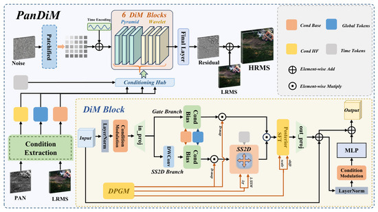
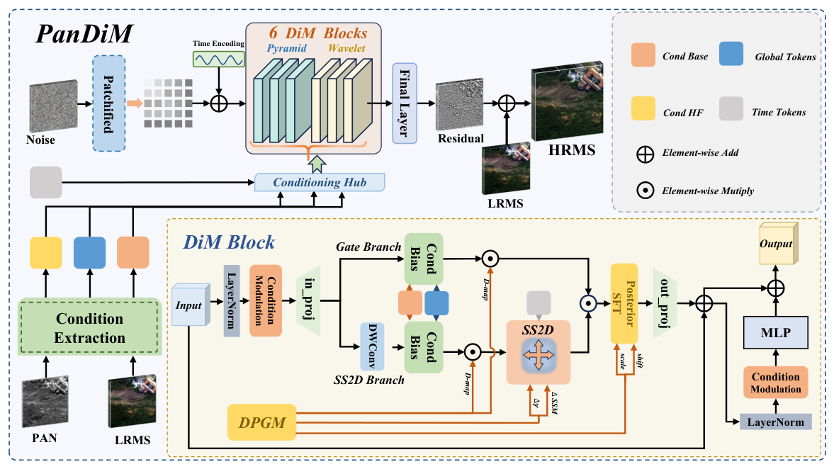
As shown in Figure 1, the overall architecture of PanDiM mainly consists of four core parts: input mapping, condition feature extraction, a stacked DiM backbone, and output reconstruction. Specifically, the noisy feature is first serialized through Patch Embedding, combined with the timestep encoding, and then fed into the denoising backbone composed of six DiM Blocks for feature updating. It is worth noting that these six DiM Blocks are divided into two stages, namely Pyramid and Wavelet, aiming to achieve more hierarchical feature representation. Finally, the output of the backbone is mapped and then added element-wise to the upsampled LRMS to generate the final HRMS image.

Figure 1. Overall framework of PanDiM. It mainly consists of Condition Extraction and a backbone denoising network with six DiM Blocks. The input noise is first patchified and injected with time encoding before being fed into the main network. Meanwhile, PAN and LRMS images are processed by the condition extraction branch to generate structured conditions, including Cond Base, Cond HF, and Global Tokens, which are injected into the DiM Blocks together with Time Tokens. Inside each DiM Block, the input features are first processed by condition modulation and then divided into the Gate Branch and the SS2D Branch. At the same time, DPGM generates the degradation map, SSM offsets, and basic affine parameters to adaptively guide feature updating in SS2D, and further performs deep fusion through Posterior SFT. Finally, the network predicts the high-frequency Residual through the Final Layer and adds it to LRMS to obtain a high-fidelity HRMS image.

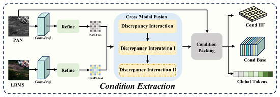
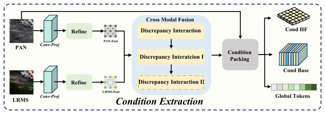
Different from the conventional practice of directly concatenating the original LRMS or PAN image into the backbone input, As shown in Figure 2, PanDiM adopts a structured condition injection strategy. In the condition extraction branch, multimodal observations are not fused only once at the front end. Instead, they are used to generate condition variables with clear functional roles for the layer-wise denoising task. Specifically, these variables include Cond Base for basic modulation at the current layer, Cond HF for retaining high-frequency detail cues, and Global Tokens for providing global semantic constraints. In addition, Time Tokens generated from the diffusion timestep encoding are also collected together. These features are jointly integrated into the Conditioning Hub and serve as control variables deeply coupled with the intra-layer state update, taking effect collaboratively in subsequent DiM Blocks.

Figure 2. Overall architecture of Condition Extraction.

As the core computational unit of the network, the DiM Block performs refined feature updating and modulation. Inside the module, the input features are first processed by Condition Modulation and then divided into the Gate Branch and the SS2D Branch through the projection layer. After introducing depthwise separable convolution to extract local features, the main branch and the gate branch both use Cond Base and Global Tokens to perform conditional bias. Meanwhile, DPGM generates dynamic degradation maps, which are applied to the activation nodes of the two branches, and outputs specific control parameters to deeply regulate the internal state of SS2D. The two branches are then coupled through element-wise multiplication and further processed by the Degradation-Guided Spatial Feature Transform layer, whose scale and shift parameters are provided by DPGM. After that, the features pass through the output projection and form a residual connection with the input. Finally, the current-layer update is completed through an MLP feed-forward network with condition modulation.

3.3. Degradation-Posterior Guidance Module

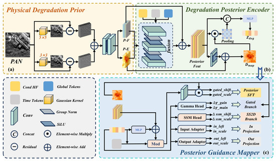
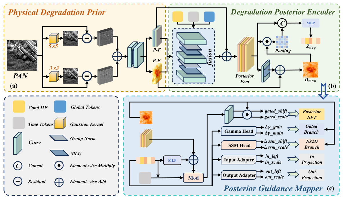
Although general condition modulation based only on Cond Base and Cond HF can provide basic condition information for the current layer, it is still difficult to explicitly distinguish the reliability of details at different spatial positions or determine the strength with which these details should participate in state updating. To this end, we propose DPGM. Unlike conventional approaches that directly predict unified modulation parameters from conditional features, DPGM adopts a posterior-style evidence fusion strategy based on a “physics-driven, learning-mapped” paradigm. Specifically, it first constructs physical detail seeds from the original PAN image, then integrates them with learned conditions to form degradation-aware evidence representations, and finally maps these representations into control variables that can be directly invoked within the backbone. As shown in Figure 3, this process consists of three stages: physical degradation prior extraction, degradation posterior encoding, and posterior guidance mapping.

Figure 3. Module architecture of DPGM. (a) Physical Degradation Prior extracts dual-scale detail residuals from the PAN image using fixed Gaussian kernels and constructs physical detail evidence. (b) Degradation Posterior Encoder fuses physical priors with learned conditions, Global Tokens, and Time Tokens to generate degradation-aware posterior features. (c) Posterior Guidance Mapper converts the posterior features into degradation maps, SSM offsets, affine parameters, and projection adapters for guiding feature updating in the DiM Block.

First, in the physical degradation prior extraction stage, we extract dual-scale detail residuals from the original PAN image to explicitly construct the physical detail prior. Specifically, two fixed Gaussian kernels are used to smooth the PAN image. The small-scale kernel is set to $k_1=3, {\sigma }_1=1.0$, while the large-scale kernel is set to $k_2=5, {\sigma }_2=2.0$. The former is used to describe local edges and fine-grained texture disturbances, while the latter is used to perceive structural variations under a larger receptive field. The dual-scale detail residuals are defined as

$$\begin{array}{cc}\hfill d_s& =P-G_{3\times 3,\sigma =1.0}\left(P\right),\hfill \end{array}$$

(8)

$$\begin{array}{cc}\hfill d_l& =P-G_{5\times 5,\sigma =2.0}\left(P\right).\hfill \end{array}$$

(9)

Furthermore, we construct a physical energy map $e_{\mathrm{phys}}$ to describe the relative strength of spatial detail evidence:

$$e_{\mathrm{phys}}=\mathrm{Norm}\left(|d_s|+|d_l|\right).$$

(10)

where $d_s$ and $d_l$ denote the detail residuals at different scales, respectively. The motivation for using dual scales is that using only a single small kernel is likely to be overly sensitive to local high-frequency noise, while using only a large kernel may weaken the localization accuracy of edges. Combining the two allows the model to balance local detail sensitivity and the stability of global structure perception. In addition, in the implementation, $d_s$ and $d_l$ are normalized by channel-wise standard deviation, respectively, to suppress the interference caused by amplitude variations across different samples and regions during the construction of degradation-aware evidence. Finally, these dual-scale physical details are not directly fed into the backbone, but serve as the physical reference starting point for degradation-aware modeling.

On this basis, the degradation posterior encoder jointly encodes the above Physical Prior and Learned Condition. Specifically, the high-frequency condition Cond HF from outside the backbone, the original PAN image, Global Tokens, and Time Tokens are aligned or projected, respectively, and then fused with the physical detail seeds to obtain the degradation-aware features $f_{\mathrm{post}}$. The spatial degradation map $D_{\mathrm{map}}$ and the global degradation vector $Z_{\mathrm{deg}}$ are further generated as

$$f_{\mathrm{post}}=\mathcal{H}\left([f_{\mathrm{phys}},f_{\mathrm{learn}},f_{\mathrm{energy}},f_g,f_t]\right)+f_{\mathrm{phys}},$$

(11)

$$D_{\mathrm{map}}=0.5\sigma \left(W_m\left(f_{\mathrm{post}}\right)\right)+0.5e_{\mathrm{phys}},$$

(12)

$$Z_{\mathrm{deg}}=M_p\left([\mathrm{GAP}\left(f_{\mathrm{post}}\odot (1+D_{\mathrm{map}})\right),\mathrm{Std}\left(f_{\mathrm{post}}\right)]\right).$$

(13)

where $D_{\mathrm{map}}$ is used to describe the reliability of details at different spatial positions, while $Z_{\mathrm{deg}}$ represents the sample-level global degradation state. Therefore, the output of DPGM at this stage is not a single attention map, but a comprehensive degradation posterior that combines spatial distribution constraints with global state awareness.

Finally, the posterior guidance mapper translates the above degradation-aware features into core control variables inside the backbone. We first project $Z_{\mathrm{deg}}$ into a spatial bias and inject it into $f_{\mathrm{post}}$. Then, Time Tokens and $Z_{\mathrm{deg}}$ are concatenated and passed through an MLP to generate time-related scale and shift terms, which are used to modulate the normalized degradation-aware features. Finally, the basic affine parameters are predicted through a zero-initialized $1\times 1$ convolution layer:

$$(\mathbf{s},\mathbf{b})={\mathcal{W}}_0\left(\varphi \left(\mathrm{Norm}\left({\mathbf{f}}_{\mathrm{post}}+\mathsf{\Phi }\left(Z_{\mathrm{deg}}\right)\right)\odot (1+{\mathbf{t}}_s)+{\mathbf{t}}_b\right)\right)$$

(14)

Additionally, s and b are reweighted at each spatial position by $g_{\mathrm{post}}$, so that regions with stronger physical detail evidence receive a larger modulation strength. In addition, we use $Z_{\mathrm{deg}}$ to generate the dynamic weights $\Delta \gamma$ and ${\Delta }_{\mathrm{ssm}}$, as well as the low-rank adaptation terms on the input and output sides. Specifically, $\Delta \gamma$ is used to correct the gain strength of the gate branch and the main branch, thereby adjusting the constraint strength of condition selection. ${\Delta }_{\mathrm{ssm}}$ is used to dynamically regulate the affine parameters of the SS2D main branch, allowing them to adapt to the sample-level degradation state. The low-rank adaptation terms provide a lightweight way to perform sample-dependent correction on feature mappings. In summary, the output of DPGM is not a single affine pair, but a set of control variables covering spatial modulation, branch gain correction, SSM adjustment, and projection adaptation:

$$P^l=\{s^l,b^l,{\Delta }^l\gamma ,{\Delta }^l\mathrm{SSM},{\Delta }^l\mathrm{in},{\Delta }^l\mathrm{out},D_{\mathrm{map}}^l,Z_{\mathrm{deg}}^l\}.$$

(15)

These variables are then applied to different computational branches in the DiM Block. Through this design, DPGM establishes a complete path from physical detail seeds to degradation posterior and then to multi-level control variables. In this way, “which regions are more reliable and with what strength they should be updated” becomes an explicitly modeled problem, effectively avoiding feature misalignment and local spectral distortion that are easily caused by traditional implicit fusion.

3.4. Time-Aware Mechanism

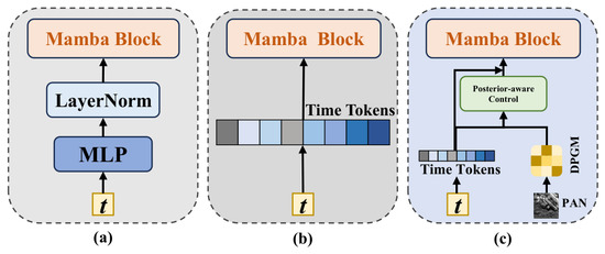
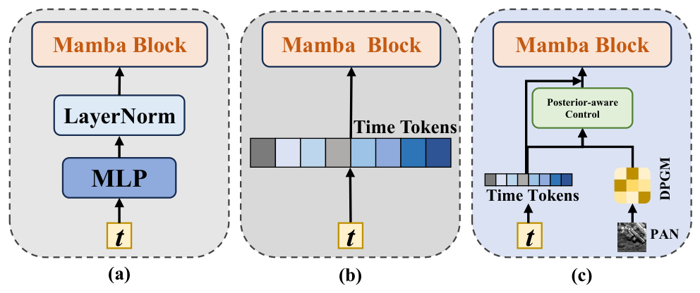
In diffusion models, temporal information is usually injected into the backbone in two ways. One way is to map the diffusion timestep through a shallow layer and directly feed it into the backbone as a condition signal [41]. The other way is to first encode the diffusion timestep into Time Tokens and then send them into the network to participate in feature updating [47]. As shown in Figure 4, although these two strategies can achieve certain effects, they essentially still treat temporal information as an auxiliary condition for computation, without directly affecting the current degradation state of the sample. As a result, when facing different noise intensities, the model lacks awareness of the differentiated degradation characteristics between modalities, which may cause misalignment during cross-modal feature fusion. To address this issue, PanDiM designs a time-aware mechanism, in which temporal information directly intervenes in both degradation posterior estimation and state-space modeling. For the diffusion timestep t, the model first encodes it and passes it through a temporal MLP to generate a layer-shared temporal representation $T_{\mathrm{emb}}$. Then, temporal information deeply acts on the backbone through two paths. On the one hand, $T_{\mathrm{emb}}$ first enters DPGM and participates in the formation of the posterior feature $F_{\mathrm{post}}$ in DPE. Then, $F_{\mathrm{post}}$ and the current degradation state $Z_{\mathrm{deg}}$ of the sample are jointly input into PGM to generate time-related posterior parameters:

$$[{\gamma }_{\mathrm{base}},{\beta }_{\mathrm{base}},\Delta \gamma ,{\Delta }_{\mathrm{ssm}}]=\mathrm{PGM}(\mathrm{DPE}\left(T_{\mathrm{emb}}\right),Z_{\mathrm{deg}}).$$

(16)

where ${\gamma }_{\mathrm{base}}$ and ${\beta }_{\mathrm{base}}$ are the basic affine parameters, while $\Delta \gamma$ and ${\Delta }_{\mathrm{ssm}}$ are dynamic weights. Together, they determine the modulation strength applied to degradation features at the current denoising stage.

Figure 4. Comparison of different time-aware mechanisms. (a) Conventional shallow condition mapping injection; (b) conventional independent Time Tokens injection; (c) the proposed deeply coupled time control mechanism. This mechanism breaks the limitation of using time only as an external stage label. By jointly using Time Tokens and the spatial degradation posterior extracted by DPGM, temporal information is promoted to a control variable that runs through the backbone and is dynamically adjusted according to the actual physical degradation degree.

On the other hand, $T_{\mathrm{emb}}$ also enters the DiM Block. The state-space-oriented MLP, denoted as ${\mathrm{MLP}}_{\mathrm{ssm}}$, generates the affine parameters ${\gamma }_{\mathrm{ss}}$ and ${\beta }_{\mathrm{ss}}$ for the SS2D main branch:

$$[{\gamma }_{\mathrm{ss}},{\beta }_{\mathrm{ss}}]={\mathrm{MLP}}_{\mathrm{ssm}}\left(T_{\mathrm{emb}}\right).$$

(17)

Finally, these time-driven affine parameters work together with the above dynamic weight ${\Delta }_{\mathrm{ssm}}$ to perform deep internal feature modulation on the input feature X in state-space modeling:

$$\tilde{X}=\mathrm{SS}2\mathrm{D}\left(({\gamma }_{\mathrm{ssm}}+\Delta \gamma )\odot X+({\beta }_{\mathrm{ssm}}+{\beta }_{\mathrm{base}}),{\Delta }_{\mathrm{ssm}}\right).$$

(18)

In this way, PanDiM can focus more on global structure recovery in the early denoising stage, while adaptively emphasizing fine local texture details in the later stage. This allows the model to significantly reduce spectral distortion while preserving clear spatial edge structures as much as possible.

3.5. Frequency-Decoupled Loss

Since PanDiM restores HRMS images in the residual space, its training objective should not be limited to a unified constraint in the global pixel domain. Instead, it needs to explicitly distinguish the preservation of low-frequency spectral information from the injection of high-frequency spatial details. To this end, in addition to the basic diffusion denoising supervision, we propose FDL, which uses a differentiable two-dimensional Gaussian low-pass filter to explicitly decompose images in the frequency domain, thereby enabling targeted optimization for features in different frequency bands. For an arbitrary input image x, its low-frequency and high-frequency components are defined as

$$\begin{array}{cc}\hfill \mathrm{LF}\left(x\right)& =G_{5\times 5,\sigma =1.5}\left(x\right),\hfill \end{array}$$

(19)

$$\begin{array}{cc}\hfill \mathrm{HF}\left(x\right)& =x-\mathrm{LF}\left(x\right).\hfill \end{array}$$

(20)

Based on this, we design two collaborative loss terms:

GT-FDL: This term directly uses the real high-resolution image as the reference and constrains the low- and high-frequency components of the predicted result, respectively:

$${\displaystyle {\mathcal{L}}_{\mathrm{GT}-\mathrm{FDL}}={\lambda }_l{∥\mathrm{LF}(\widehat{Y})-\mathrm{LF}\left(Y\right)∥}_1+{\lambda }_h{∥\mathrm{HF}(\widehat{Y})-\mathrm{HF}\left(Y\right)∥}_1.}$$

(21)

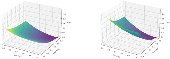
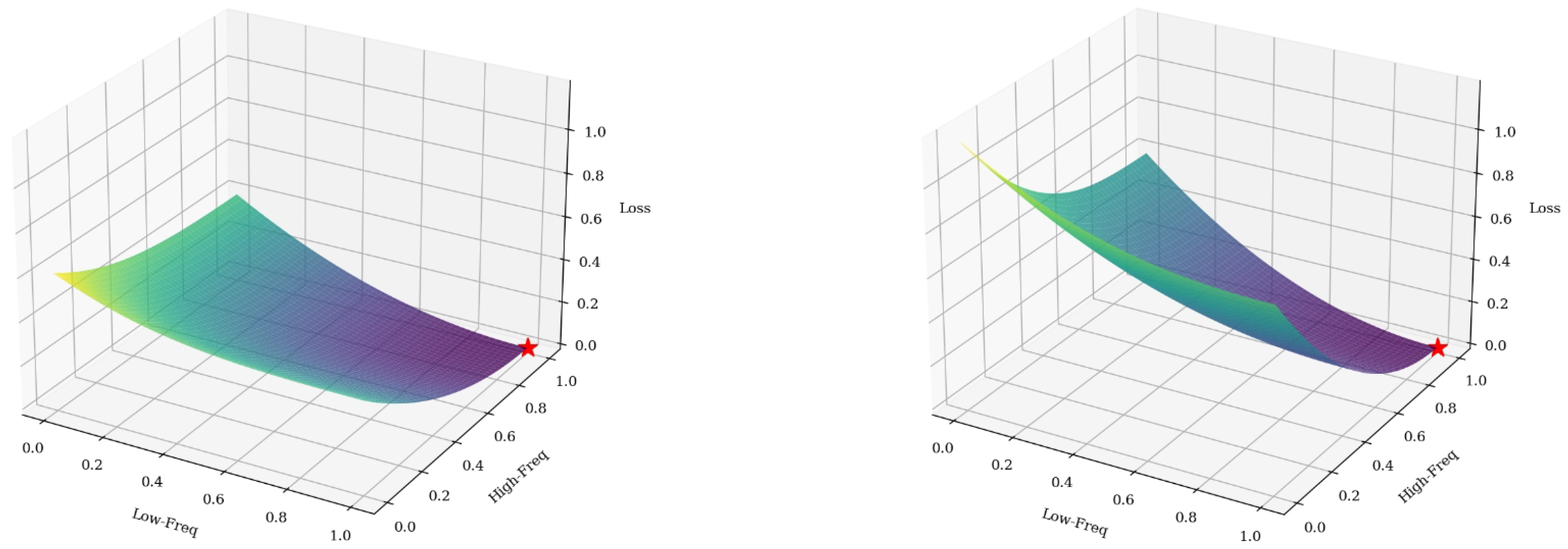
In this paper, the weight of the low-frequency term is set to 1.0 to constrain the overall spectral consistency, while the high-frequency enhancement weight is set to ${\lambda }_h=2.0$, so that edge and texture recovery can be strengthened with a larger penalty. To more intuitively illustrate its optimization characteristics, Figure 5 compares the characteristic surfaces of the standard $L_1$ loss and GT-FDL. It can be seen that the standard $L_1$ loss responds relatively uniformly to errors in different frequency bands, whereas GT-FDL maintains stable low-frequency constraints while showing a more sensitive penalty tendency for high-frequency deviations. Therefore, it can more specifically suppress high-frequency structural errors and avoid systematic bias caused by proxy signals.

Figure 5. Visual comparison of the characteristic surfaces of different loss functions. The (left) side shows the standard L1 loss, and the (right) side shows GT-FDL.

Spatial-FDL: To further introduce the physical prior of the pansharpening task, namely “low frequency comes from multispectral images and high frequency comes from panchromatic images”, we design Spatial-FDL as an auxiliary loss. This term aligns the low-frequency component of the predicted image with the upsampled LRMS image, and aligns the high-frequency component with the PAN image:

$${\displaystyle {\mathcal{L}}_{\mathrm{Spatial}-\mathrm{FDL}}={∥\mathrm{LF}(\widehat{Y})-\mathrm{LF}\left(L\right)∥}_1+{∥{\mathrm{HF}}_{\mathrm{gray}}(\widehat{Y})-\mathrm{HF}\left(P\right)∥}_1.}$$

(22)

Here, ${\mathrm{HF}}_{\mathrm{gray}}\left(\widehat{Y}\right)$ denotes that the high-frequency component of the predicted HRMS image is first averaged along the channel dimension and then aligned with the high-frequency component of the single-channel PAN image, which effectively alleviates the dimension mismatch problem in cross-modal constraints. In the training setting, Spatial-FDL is introduced as an auxiliary physical prior term. Its initial weight is set to 0.05, and a Cosine Decay curriculum strategy is adopted to gradually reduce its influence during training. This design allows the physical prior to provide stable directional guidance mainly in the early training stage, preventing the model from falling into severe local spectral distortion at the beginning, while avoiding excessive restriction on the model’s adaptive optimization ability in the later training stage.

Through this collaborative design, GT-FDL and Spatial-FDL jointly form a hierarchical supervision mechanism, which ensures spectral fidelity while maximizing the model’s ability to perceive and reconstruct high-frequency spatial details.

4. Experiments

4.1. Experimental Platform

All our experiments are conducted on the Ubuntu 20.04.6 LTS operating system, using a single NVIDIA A10 Tensor Core GPU for model training and testing. The Python version is 3.11.14, the deep learning framework is PyTorch 2.1.0, and the CUDA version is 12.1.

4.2. Datasets

To comprehensively evaluate the performance of PanDiM, we conduct experiments on three representative remote sensing datasets from PanCollection [48], including WorldView-3 (WV3), which contains eight spectral bands, GaoFen-2 (GF2), which contains four spectral bands, and QuickBird (QB). Data simulation is strictly conducted following the Wald protocol, which is widely adopted in pansharpening, to ensure a fair reference-based evaluation setting across different datasets [49]. The WV3 dataset contains 9714 training pairs, where the MS size is $16\times 16\times 8$ and the PAN size is $64\times 64\times 1$. The GF2 dataset contains 19,809 training pairs, and the QB dataset contains 17,139 training pairs. For both GF2 and QB, the LRMS size is $16\times 16\times 4$, and the PAN size is $64\times 64\times 1$. To fully test the model performance, we follow the standard split of PanCollection on all three datasets. Specifically, an independent reduced-resolution test set, containing 20 image pairs of size $256\times 256$, is used for reference-based metric evaluation and visual analysis. In addition, a full-resolution test set, containing 20 image pairs of size $512\times 512$, is used for visual evaluation and no-reference metric evaluation under real scenarios.

4.3. Hyperparameters and Evaluation Metrics

PanDiM is trained for a total of 50,000 iterations, with both the patch size and batch size set to eight. The number of DiM Blocks is set to six, and the inner channel dimension is set to 16. We use the AdamW optimizer with a weight decay of $1\times {10}^{-4}$, and the learning rate is set to $1\times {10}^{-4}$. Meanwhile, after 20,000 steps, an EMA mechanism with a decay rate of 0.995 is introduced to stabilize the model weights. For the FDL function, the high-frequency enhancement coefficient is set to 2.0 to strengthen edge recovery, and the peak weight of the spatial frequency prior is set to 0.05. During the first 60% of training, this term maintains full-weight guidance to support the initial construction of structural information, and then its weight is smoothly reduced through cosine annealing. To comprehensively evaluate the reconstruction quality of the fusion results, we use SAM, ERGAS, and PSNR as the unified evaluation metrics in the reduced-resolution experiments. In particular, Q8 is additionally adopted for the WV3 dataset, while Q4 is additionally adopted for the GF2 and QB datasets. In the full-resolution experiments, $D_{\lambda }$, $D_s$, and HQNR are used for performance [50].

4.4. Reduced-Resolution Evaluation

To verify the effectiveness of PanDiM, we compare it with various representative traditional methods and deep learning methods. Specifically, we select multiple methods, including but not limited to traditional methods such as MTF-FS-GLP [51] and TV [52], as well as deep learning methods such as PanNet [22] and CANConv [25]. All comparison methods are reproduced, trained, and evaluated based on their publicly available code under the same datasets and experimental settings, so as to ensure the fairness of comparison. Table 1 shows the comparison results of PanDiM and other mainstream methods on the WV3 dataset. As shown in the table, on the WV3 dataset, PanDiM achieves the best results on all four metrics, including SAM, ERGAS, Q8, and PSNR, outperforming the second-best method by 0.099, 0.036, 0.011, and 0.211 dB, respectively. Figure 6 presents the reduced-resolution fusion results and ground-truth residual maps of PanDiM and other models on the WV3 dataset. It can be seen that the reconstruction results of PanDiM are overall closer to the reference images and contain fewer high-error response regions, showing excellent fusion performance.

Table 1. Quantitative evaluation results of PanDiM and representative methods on the WV3 dataset at reduced and full resolutions. The best and second-best results are highlighted in red and blue, respectively.

Method	Reduced-Resolution Metrics				Full-Resolution Metrics
	SAM ↓	ERGAS ↓	${\mathit{Q}}_{\mathbf{8}}\mathbf{\uparrow }$	PSNR ↑	${\mathit{D}}_{\mathit{\lambda }}\mathbf{\downarrow }$	${\mathit{D}}_{\mathit{s}}$ ↓	HQNR ↑
EXP	5.838 ± 1.714	7.129 ± 1.613	0.603 ± 0.091	27.077 ± 2.430	0.0232 ± 0.0066	0.0813 ± 0.0318	0.8975 ± 0.0362
MTF-GLP-FS [51]	5.323 ± 1.655	4.645 ± 1.444	0.818 ± 0.101	30.921 ± 1.430	0.0625 ± 0.0235	0.0730 ± 0.0356	0.8698 ± 0.0531
TV [52]	5.598 ± 1.684	4.768 ± 1.267	0.794 ± 0.116	30.542 ± 1.507	0.0197 ± 0.0078	0.0630 ± 0.0289	0.9187 ± 0.0347
BDSD-PC [53]	5.467 ± 1.719	4.655 ± 1.467	0.812 ± 0.106	30.947 ± 1.445	0.0502 ± 0.0165	0.0202 ± 0.0108	0.9307 ± 0.0248
CVPR2019 [54]	5.425 ± 1.531	5.623 ± 1.342	0.734 ± 0.093	29.152 ± 2.140	0.0234 ± 0.0061	0.0393 ± 0.0227	0.9383 ± 0.0269
LRTCFPan [55]	4.670 ± 1.277	4.232 ± 1.277	0.836 ± 0.097	31.818 ± 1.535	0.0163 ± 0.0058	0.0484 ± 0.0217	0.9362 ± 0.0258
PNN [21]	4.344 ± 1.040	3.887 ± 1.063	0.835 ± 0.105	32.685 ± 1.650	0.0328 ± 0.0142	0.0515 ± 0.0228	0.9177 ± 0.0343
PanNet [22]	4.033 ± 0.821	3.472 ± 1.019	0.853 ± 0.106	33.566 ± 1.841	0.0229 ± 0.0069	0.0539 ± 0.0168	0.9245 ± 0.0212
DiCNN [23]	3.566 ± 0.684	2.659 ± 0.614	0.891 ± 0.090	35.686 ± 1.659	0.0346 ± 0.0108	0.0464 ± 0.0166	0.9207 ± 0.0246
FusionNet [56]	3.337 ± 0.637	2.451 ± 0.581	0.896 ± 0.091	36.485 ± 1.576	0.0225 ± 0.0083	0.0355 ± 0.0169	0.9429 ± 0.0230
DCFNet [57]	3.375 ± 0.624	2.741 ± 0.603	0.882 ± 0.101	35.371 ± 1.906	0.0336 ± 0.0119	0.0333 ± 0.0045	0.9342 ± 0.0131
LAGConv [24]	3.130 ± 0.557	2.383 ± 0.581	0.904 ± 0.088	36.820 ± 1.835	0.0306 ± 0.0107	0.0439 ± 0.0147	0.9269 ± 0.0222
HMPNet [58]	3.197 ± 0.579	2.456 ± 0.706	0.903 ± 0.092	36.511 ± 1.565	0.0251 ± 0.0105	0.0317 ± 0.0044	0.9460 ± 0.0124
CMT [59]	3.380 ± 0.607	2.678 ± 0.618	0.874 ± 0.101	35.658 ± 1.737	0.0264 ± 0.0081	0.0417 ± 0.0097	0.9330 ± 0.0157
ARConv [26]	3.269 ± 0.616	2.548 ± 0.698	0.901 ± 0.088	36.146 ± 1.787	0.0169 ± 0.0072	0.0313 ± 0.0111	0.9523 ± 0.0162
CANConv [25]	3.262 ± 0.621	2.308 ± 0.524	0.901 ± 0.082	36.606 ± 1.508	0.0165 ± 0.0064	0.0383 ± 0.0043	0.9458 ± 0.0088
Pan-Mamba [37]	4.293 ± 0.899	3.698 ± 0.887	0.861 ± 0.098	32.807 ± 1.643	0.0287 ± 0.0109	0.0573 ± 0.0217	0.9158 ± 0.0301
FusionMamba [38]	3.517 ± 0.682	3.075 ± 0.690	0.883 ± 0.091	34.293 ± 2.219	0.0253 ± 0.0080	0.0454 ± 0.0047	0.9304 ± 0.0098
CrossDiff [46]	3.621 ± 0.751	2.729 ± 0.680	0.884 ± 0.100	35.442 ± 1.350	0.0277 ± 0.0208	0.0232 ± 0.0098	0.9497 ± 0.0221
PanDiT [20]	3.721 ± 0.705	2.823 ± 0.600	0.877 ± 0.107	35.232 ± 2.023	0.0167 ± 0.0061	0.0392 ± 0.0141	0.9448 ± 0.0185
PanDiM	3.031 ± 0.566	2.272 ± 0.489	0.915 ± 0.090	37.031 ± 1.822	0.0128 ± 0.0046	0.0301 ± 0.0101	0.9574 ± 0.0128

Figure 6. Visualization of fusion results of PanDiM and other comparison methods on WV3. It can be seen that PanDiM achieves the best spectral fidelity and detail restoration, and its residual map shows a significantly lower error rate than those of other methods.

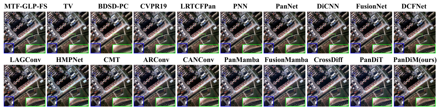
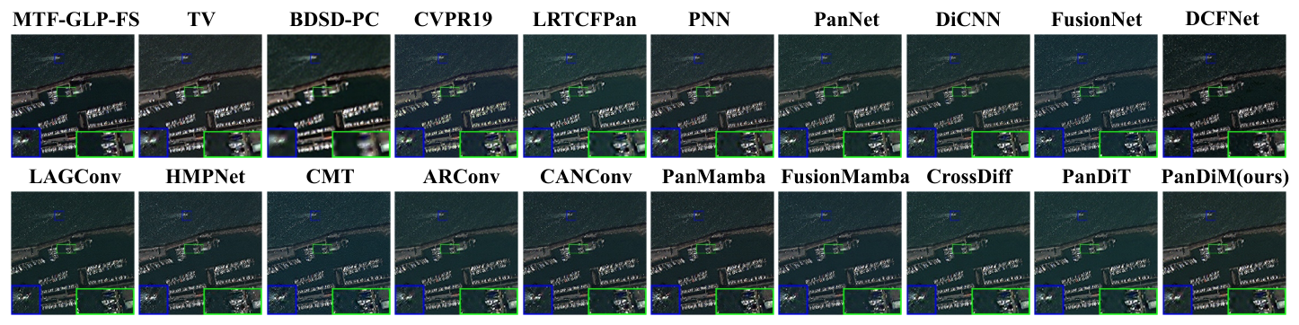
In addition, PanDiM also shows strong performance on the GF2 and QB datasets. Table 2 and Table 3 present the evaluation results of PanDiM and other mainstream methods on the GF2 and QB datasets, respectively. The SAM, ERGAS, Q4, and PSNR values of PanDiM reach 0.742/4.344, 0.627/3.594, 0.984/0.939, and 43.702/38.012, respectively, achieving the best performance on most metrics. Figure 7 and Figure 8 present the visual inference results of PanDiM and other methods on the GF2 and QB datasets. PanDiM still achieves superior fusion performance. In particular, it exhibits remarkable reconstruction ability in regions containing land–water boundary edges and densely distributed ships in ports, where complex spatial details are clearly restored.

Table 2. Quantitative evaluation results of PanDiM and representative methods on the GF2 dataset at reduced and full resolutions. The best and second-best results are highlighted in red and blue, respectively.

Method	Reduced-Resolution Metrics				Full-Resolution Metrics
	SAM ↓	ERGAS ↓	${\mathit{Q}}_{\mathbf{8}}\uparrow$	PSNR ↑	${\mathit{D}}_{\mathit{\lambda }}$ ↓	${\mathit{D}}_{\mathit{s}}$ ↓	HQNR ↑
EXP	1.852 ± 0.355	2.406 ± 0.476	0.797 ± 0.044	31.944 ± 1.937	0.0180 ± 0.0081	0.0957 ± 0.0209	0.8881 ± 0.0228
MTF-GLP-FS [51]	1.680 ± 0.349	1.620 ± 0.362	0.890 ± 0.026	35.286 ± 1.944	0.0749 ± 0.0299	0.1535 ± 0.0278	0.7833 ± 0.0406
TV [52]	1.816 ± 0.362	1.988 ± 0.429	0.852 ± 0.038	33.640 ± 2.025	0.0346 ± 0.0137	0.1429 ± 0.0282	0.8276 ± 0.0348
BDSD-PC [53]	1.720 ± 0.319	1.684 ± 0.395	0.886 ± 0.031	35.020 ± 2.049	0.0388 ± 0.0153	0.0413 ± 0.0112	0.9216 ± 0.0200
CVPR2019 [54]	1.687 ± 0.282	1.904 ± 0.357	0.836 ± 0.053	33.773 ± 1.397	0.1387 ± 0.0470	0.1488 ± 0.0316	0.7332 ± 0.0504
LRTCFPan [55]	1.315 ± 0.283	1.301 ± 0.313	0.932 ± 0.033	37.347 ± 2.073	0.0333 ± 0.0270	0.0935 ± 0.0157	0.8762 ± 0.0250
PNN [21]	1.106 ± 0.215	1.079 ± 0.233	0.957 ± 0.013	38.938 ± 1.985	0.0309 ± 0.0126	0.0930 ± 0.0136	0.8789 ± 0.0160
PanNet [22]	1.189 ± 0.226	1.138 ± 0.228	0.950 ± 0.017	38.475 ± 1.821	0.0280 ± 0.0129	0.0851 ± 0.0146	0.8893 ± 0.0170
DiCNN [23]	1.070 ± 0.209	1.100 ± 0.228	0.957 ± 0.011	38.709 ± 2.034	0.0349 ± 0.0140	0.0970 ± 0.0122	0.8715 ± 0.0168
FusionNet [56]	0.996 ± 0.195	1.010 ± 0.195	0.961 ± 0.012	39.414 ± 1.921	0.0364 ± 0.0143	0.1003 ± 0.0135	0.8669 ± 0.0191
DCFNet [57]	1.051 ± 0.196	1.071 ± 0.210	0.963 ± 0.014	39.197 ± 2.011	0.0326 ± 0.0343	0.0580 ± 0.0138	0.9109 ± 0.0243
LAGConv [24]	0.765 ± 0.129	0.681 ± 0.110	0.980 ± 0.009	42.773 ± 1.411	0.0263 ± 0.0123	0.0759 ± 0.0105	0.8997 ± 0.0160
HMPNet [58]	1.036 ± 0.141	0.876 ± 0.132	0.972 ± 0.014	40.637 ± 1.633	0.0612 ± 0.0424	0.0812 ± 0.0124	0.8626 ± 0.0407
CMT [59]	1.175 ± 0.232	1.156 ± 0.224	0.959 ± 0.012	38.590 ± 1.918	0.0271 ± 0.0095	0.0641 ± 0.0092	0.9106 ± 0.0118
ARConv [26]	1.128 ± 0.243	0.997 ± 0.183	0.937 ± 0.018	38.695 ± 1.762	0.0281 ± 0.0119	0.0576 ± 0.0199	0.9159 ± 0.0254
CANConv [25]	0.710 ± 0.139	0.647 ± 0.127	0.982 ± 0.007	43.258 ± 1.746	0.0175 ± 0.0094	0.0506 ± 0.0084	0.9309 ± 0.0106
Pan-Mamba [37]	1.452 ± 0.302	1.569 ± 0.260	0.882 ± 0.034	34.174 ± 1.916	0.0237 ± 0.0112	0.0868 ± 0.0221	0.8916 ± 0.0244
FusionMamba [38]	1.664 ± 0.291	1.538 ± 0.266	0.888 ± 0.035	35.072 ± 1.815	0.0437 ± 0.0377	0.0693 ± 0.0285	0.8898 ± 0.0414
CrossDiff [46]	1.355 ± 0.238	1.255 ± 0.198	0.906 ± 0.035	36.676 ± 1.416	0.0343 ± 0.0268	0.0938 ± 0.0209	0.8750 ± 0.0304
PanDiT [20]	1.117 ± 0.223	1.139 ± 0.236	0.935 ± 0.020	37.983 ± 1.807	0.0348 ± 0.0217	0.0472 ± 0.0162	0.9196 ± 0.0242
PanDiM	0.742 ± 0.202	0.627 ± 0.152	0.984 ± 0.015	43.702 ± 1.510	0.0171 ± 0.0245	0.0348 ± 0.0147	0.9395 ± 0.0221

Table 3. Quantitative evaluation results of PanDiM and representative methods on the QB dataset at reduced and full resolutions. The best and second-best results are highlighted in red and blue, respectively.

Method	Reduced-Resolution Metrics				Full-Resolution Metrics
	SAM ↓	ERGAS ↓	${\mathit{Q}}_{\mathbf{8}}\mathbf{\uparrow }$	PSNR ↑	${\mathit{D}}_{\mathit{\lambda }}\mathbf{\downarrow }$	${\mathit{D}}_{\mathit{s}}$ ↓	HQNR ↑
EXP	8.557 ± 1.746	12.010 ± 1.573	0.578 ± 0.079	27.790 ± 2.922	0.0436 ± 0.0089	0.1502 ± 0.0167	0.8127 ± 0.0204
MTF-GLP-FS [51]	7.867 ± 1.667	7.449 ± 0.561	0.834 ± 0.096	31.813 ± 2.232	0.1975 ± 0.0334	0.1636 ± 0.0483	0.6722 ± 0.0577
TV [52]	8.524 ± 1.845	9.749 ± 1.095	0.702 ± 0.105	29.547 ± 2.705	0.0465 ± 0.0146	0.1500 ± 0.0238	0.8108 ± 0.0337
BDSD-PC [53]	8.184 ± 1.826	7.614 ± 0.592	0.829 ± 0.099	31.646 ± 2.307	0.1066 ± 0.0264	0.0614 ± 0.0171	0.8389 ± 0.0377
CVPR2019 [54]	8.449 ± 1.775	7.714 ± 0.610	0.827 ± 0.098	31.501 ± 2.315	0.0765 ± 0.0354	0.1595 ± 0.0363	0.7774 ± 0.0600
LRTCFPan [55]	7.285 ± 1.599	7.028 ± 0.623	0.853 ± 0.094	32.321 ± 2.406	0.0276 ± 0.0098	0.1012 ± 0.0294	0.8742 ± 0.0361
PNN [21]	5.813 ± 1.016	6.582 ± 0.546	0.876 ± 0.099	32.933 ± 2.397	0.1048 ± 0.0112	0.1305 ± 0.0310	0.7786 ± 0.0352
PanNet [22]	5.768 ± 0.998	6.326 ± 0.460	0.877 ± 0.101	33.256 ± 2.200	0.0744 ± 0.0158	0.1243 ± 0.0270	0.8110 ± 0.0371
DiCNN [23]	5.385 ± 0.924	5.089 ± 0.378	0.905 ± 0.101	35.137 ± 1.919	0.1100 ± 0.0176	0.1107 ± 0.0204	0.7918 ± 0.0321
FusionNet [56]	4.934 ± 0.822	4.238 ± 0.258	0.922 ± 0.099	36.708 ± 1.743	0.0634 ± 0.0194	0.0457 ± 0.0191	0.8941 ± 0.0344
DCFNet [57]	4.743 ± 0.523	4.426 ± 0.863	0.911 ± 0.145	36.237 ± 0.857	0.0902 ± 0.0287	0.0328 ± 0.0076	0.8799 ± 0.0265
LAGConv [24]	4.536 ± 0.754	3.728 ± 0.310	0.934 ± 0.092	37.838 ± 1.716	0.0623 ± 0.0136	0.0809 ± 0.0222	0.8616 ± 0.0125
HMPNet [58]	4.830 ± 0.831	4.127 ± 0.305	0.930 ± 0.086	36.933 ± 1.895	0.0426 ± 0.0191	0.0828 ± 0.0186	0.8778 ± 0.0099
CMT [59]	5.252 ± 0.808	5.432 ± 0.798	0.903 ± 0.101	34.660 ± 2.139	0.0596 ± 0.0104	0.0455 ± 0.0099	0.8976 ± 0.0176
ARConv [26]	5.473 ± 1.426	4.282 ± 0.840	0.886 ± 0.109	36.067 ± 2.445	0.0515 ± 0.0163	0.0426 ± 0.0235	0.0984 ± 0.0364
CANConv [25]	4.522 ± 0.776	3.795 ± 0.282	0.935 ± 0.091	37.894 ± 1.789	0.0388 ± 0.0144	0.0913 ± 0.0216	0.8732 ± 0.0141
Pan-Mamba [37]	5.358 ± 0.945	5.588 ± 0.474	0.914 ± 0.083	34.316 ± 1.855	0.0512 ± 0.0257	0.0397 ± 0.0101	0.9113 ± 0.0311
FusionMamba [38]	6.530 ± 1.324	8.841 ± 1.052	0.819 ± 0.078	30.390 ± 2.769	0.0670 ± 0.0262	0.0435 ± 0.0094	0.8925 ± 0.0308
CrossDiff [46]	5.753 ± 0.967	5.097 ± 0.458	0.903 ± 0.105	35.132 ± 1.651	0.0337 ± 0.0104	0.0465 ± 0.0174	0.9215 ± 0.0254
PanDiT [20]	5.385 ± 0.991	4.797 ± 0.420	0.921 ± 0.089	35.637 ± 2.321	0.0445 ± 0.0147	0.0666 ± 0.0278	0.8923 ± 0.0386
PanDiM	4.344 ± 0.816	3.594 ± 0.301	0.939 ± 0.089	38.012 ± 1.992	0.0264 ± 0.0063	0.0299 ± 0.0163	0.9446 ± 0.0210

Figure 7. Visualization of reduced-resolution fusion results of PanDiM and other comparison methods on GF2.

Figure 8. Visualization of reduced-resolution fusion results of PanDiM and other comparison methods on QB.

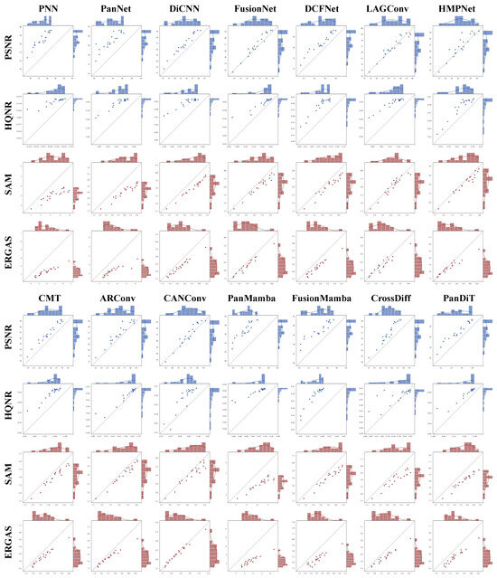
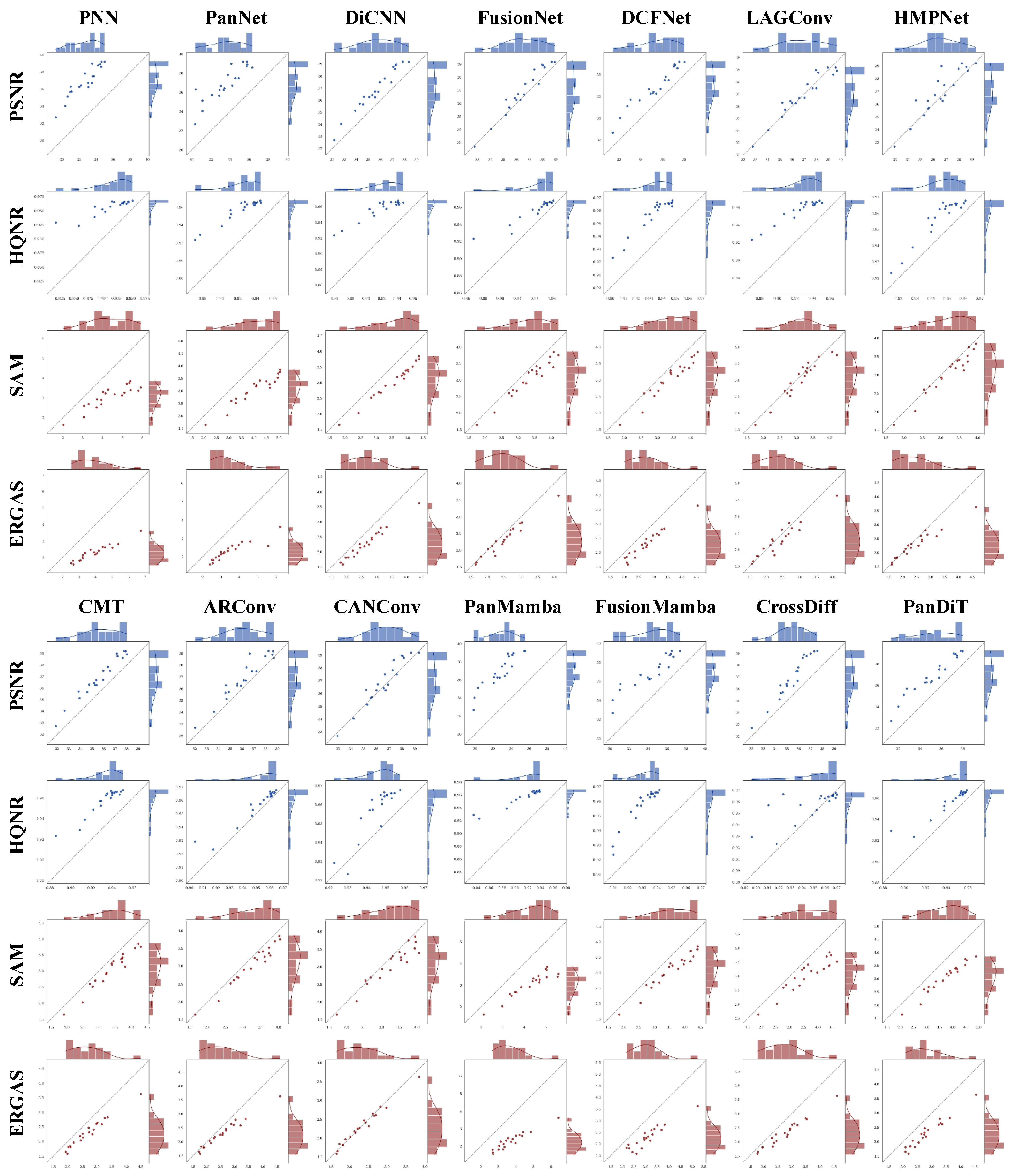
On this basis, to exclude the potential influence of a few advantageous samples in average metric evaluation, we further conduct sample-wise joint scatter comparisons on four metrics, namely PSNR, HQNR, SAM, and ERGAS, based on the reduced-resolution evaluation results on the WV3 dataset. Specifically, in each comparison group, the metric values of each comparison method are used as the horizontal axis, while the metric values of PanDiM are used as the vertical axis. A diagonal dashed line is used as the reference boundary, indicating comparable performance between the two methods. Meanwhile, marginal histograms are used to show the distribution differences in metric scores between the two methods. Figure 9 shows the comparison results between PanDiM and other methods on the WV3 dataset. It can be seen that, for each metric, PanDiM maintains an advantage on almost every test sample in the dataset, showing a general performance advantage and further demonstrating the excellent effectiveness of this framework in the field of pansharpening.

Figure 9. Histogram–scatter plots comparing PanDiM with other comparison methods in terms of PSNR, HQNR, SAM, and ERGAS. For PSNR and HQNR, if the scatter points are more concentrated above the diagonal line, and for SAM and ERGAS, if the scatter points are generally located below the diagonal line, this indicates that PanDiM has stronger advantages in spectral fidelity and overall error control.

In particular, to further convert the sample-level advantages into quantitative statistical evidence, we conducted paired Wilcoxon signed-rank tests on PSNR and HQNR. For each competing method, we calculated the per-sample difference on the WV3 test dataset as follows:

$$d_i^{\left(m\right)}=M_i^{\mathrm{PanDiM}}-M_i^m, M\in \{\mathrm{PSNR},\mathrm{HQNR}\},$$

(23)

where i denotes the sample index. Since both PSNR and HQNR are higher-is-better metrics, $d_i^{\left(m\right)}>0$ indicates that PanDiM outperforms the corresponding method on the i-th sample. The null hypothesis is defined as $H_0:\mathrm{median}\left(d^{\left(m\right)}\right)=0$, while the alternative hypothesis is $H_1:\mathrm{median}\left(d^{\left(m\right)}\right)>0$, with the significance level set to 0.05. Table 4 reports the test results of PanDiM against all learning-based comparison models included in the statistical analysis, where $\Delta$ denotes the average per-sample advantage of PanDiM over the corresponding method, and Wins/Losses/Ties indicate the sample-wise win–loss–tie counts over the 20 test samples.

Table 4. Paired Wilcoxon signed-rank test results on PSNR and HQNR between PanDiM and comparison methods on the WV3 dataset.

Method	PSNR				HQNR
	$\mathbf{\Delta }$	p-Value	W/L/T	Sig.	$\mathbf{\Delta }$	p-Value	W/L/T	Sig.
PNN [21]	4.241467	$9.6\times {10}^{-5}$	20/0/0	Yes	0.039705	$9.6\times {10}^{-5}$	20/0/0	Yes
PanNet [22]	3.361172	$9.6\times {10}^{-5}$	20/0/0	Yes	0.032976	$9.6\times {10}^{-5}$	20/0/0	Yes
DiCNN [23]	1.240843	$9.6\times {10}^{-5}$	20/0/0	Yes	0.036700	$9.6\times {10}^{-5}$	20/0/0	Yes
FusionNet [56]	0.441936	$8.34\times {10}^{-4}$	16/4/0	Yes	0.014513	$9.6\times {10}^{-5}$	20/0/0	Yes
DCFNet [57]	1.555833	$9.6\times {10}^{-5}$	20/0/0	Yes	0.023196	$9.6\times {10}^{-5}$	20/0/0	Yes
LAGConv [24]	0.102803	0.4898	11/9/0	No	0.030524	$9.6\times {10}^{-5}$	20/0/0	Yes
HMPNet [58]	0.411773	0.0967	11/9/0	No	0.011434	$9.6\times {10}^{-5}$	20/0/0	Yes
CMT [59]	1.269150	$9.6\times {10}^{-5}$	20/0/0	Yes	0.024404	$9.6\times {10}^{-5}$	20/0/0	Yes
ARConv [26]	0.780931	$1.12\times {10}^{-4}$	19/1/0	Yes	0.005107	$9.6\times {10}^{-5}$	20/0/0	Yes
CANConv [25]	0.316837	0.0458	12/8/0	Yes	0.011646	$1.75\times {10}^{-4}$	19/1/0	Yes
Pan-Mamba [37]	4.120218	$9.6\times {10}^{-5}$	20/0/0	Yes	0.041609	$9.6\times {10}^{-5}$	20/0/0	Yes
FusionMamba [38]	2.633721	$9.6\times {10}^{-5}$	20/0/0	Yes	0.027041	$9.6\times {10}^{-5}$	20/0/0	Yes
CrossDiff [46]	1.484357	$9.6\times {10}^{-5}$	20/0/0	Yes	0.007698	0.1126	11/9/0	No
PanDiT [20]	1.694582	$9.6\times {10}^{-5}$	20/0/0	Yes	0.012661	$9.6\times {10}^{-5}$	20/0/0	Yes

As shown in Table 4, in terms of PSNR, PanDiM demonstrates statistically significant advantages over all comparison methods except HMPNet and LAGConv ($p<0.05$). In particular, the p-values against CrossDiff and PanDiT are both $9.6\times {10}^{-5}$, with PanDiM outperforming them on all 20 test samples.

For HQNR, PanDiM achieves statistically significant advantages over all comparison models except CrossDiff. Notably, compared with representative methods such as PanDiT and LAGConv, PanDiM maintains sample-wise superiority across all 20 samples. These results are consistent with the trends observed in our joint scatter plots, further indicating that the advantages of PanDiM are not driven by only a few favorable samples but exhibit strong statistical stability.

4.5. Full-Resolution Evaluation

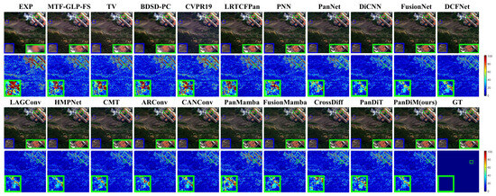
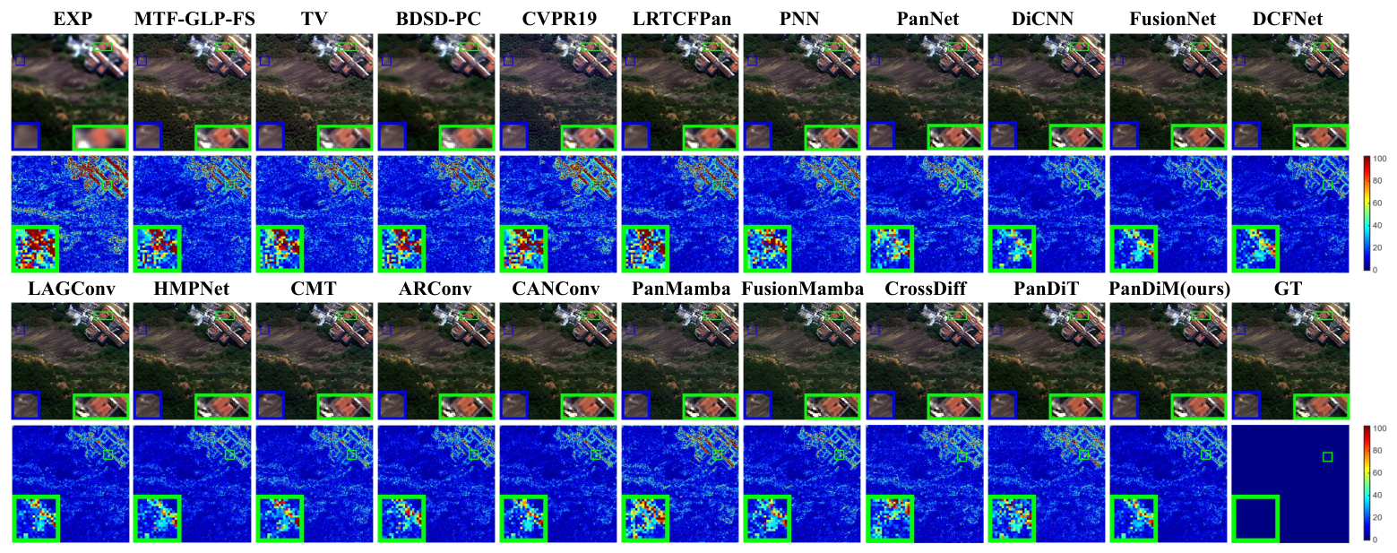
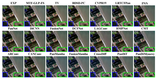
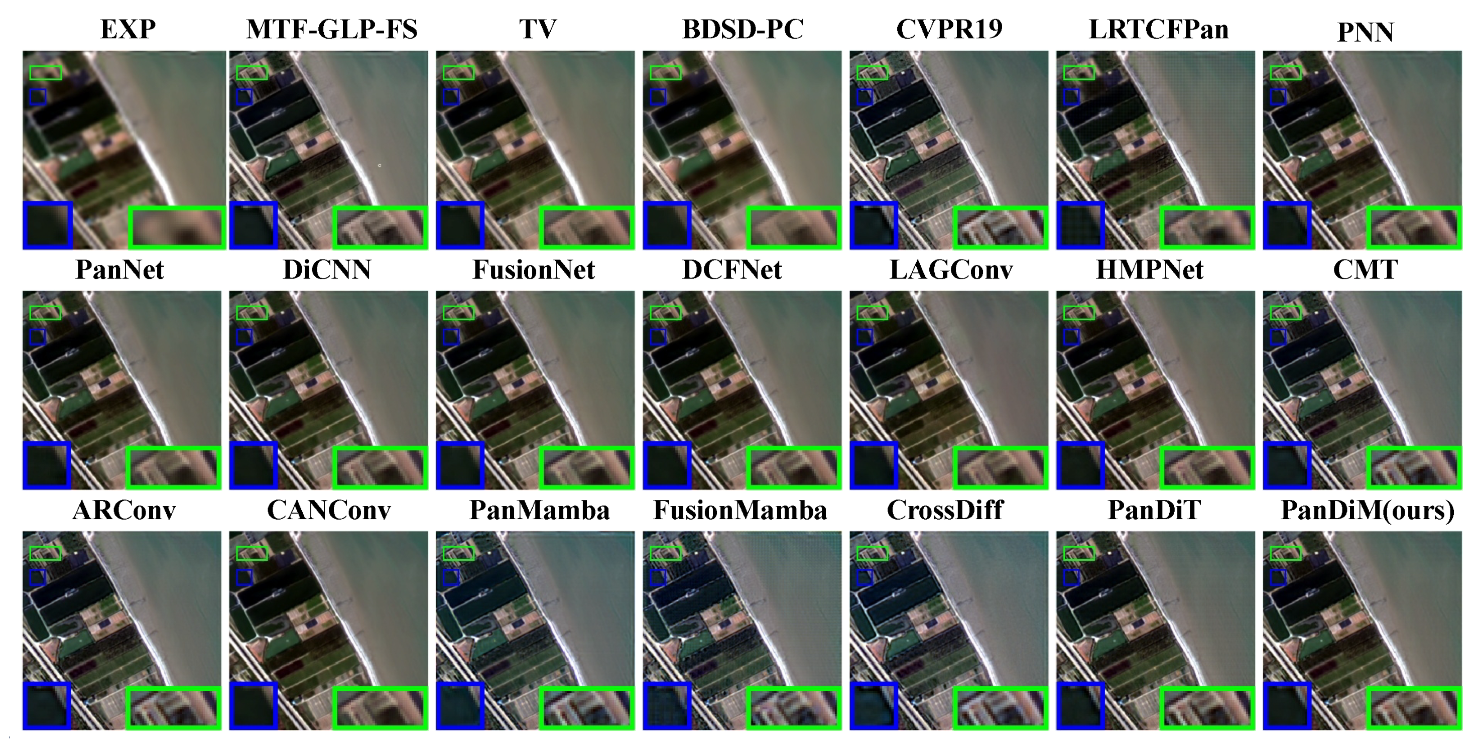
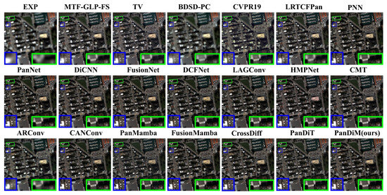
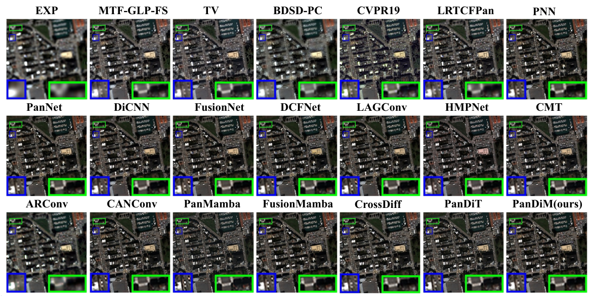
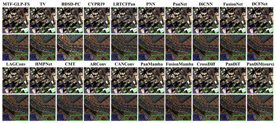
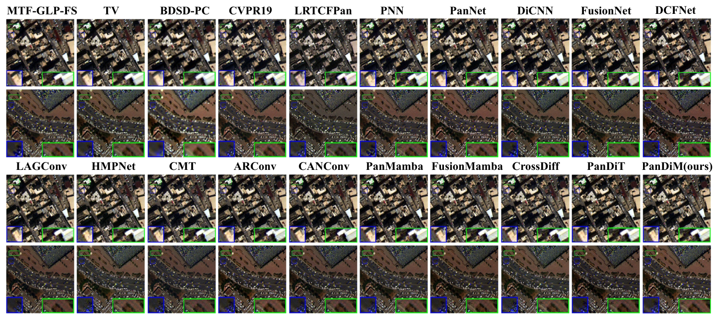
To verify the practical fusion performance of PanDiM under no-reference conditions, we further conduct full-resolution experiments on the WV3, GF2, and QB datasets. As shown in Table 1, Table 2 and Table 3, PanDiM still achieves the best results on multiple metrics. Specifically, on the WV3 dataset, PanDiM obtains 0.0128 and 0.9574 on $D_{\lambda }$ and HQNR, respectively, outperforming the other methods by 27.34–388.28% and 0.53–10.07%. Meanwhile, PanDiM reaches 0.0301 on the spatial distortion metric $D_s$, ranking second-best among all methods. In addition, for the full-resolution evaluation results on the GF2 and QB datasets, PanDiM also achieves consistently leading performance. Overall, these results demonstrate that PanDiM delivers excellent reconstruction quality and is well suited for remote sensing image pansharpening. To further illustrate the reconstruction differences among different methods in real-resolution scenarios, we visualize the inference results of all methods on the three datasets, as shown in Figure 10, Figure 11 and Figure 12.

Figure 10. Visualization of full-resolution fusion results on WV3.

Figure 11. Visualization of full-resolution fusion results on GF2.

Figure 12. Visualization of full-resolution fusion results on QB.

4.6. Model Configuration

To analyze the rationality of the experimental configuration in PanDiM, we conduct a model configuration analysis on the WV3 dataset, where the effects of patch size, the number of DiM Blocks, and model width are examined, respectively. The default configuration is consistent with the settings described in Section 4.3. Unless otherwise specified, bold values in the following configuration and ablation tables indicate the best results within the corresponding comparison group. As shown in Table 5, the three groups of configurations show consistent trends. A patch size of eight achieves the best performance, indicating that the current input patch setting is more suitable for multi-scale information modeling. When the number of DiM Blocks increases from four to six, the performance improves obviously, while further increasing it to eight brings limited gains. This suggests that the current depth is already sufficient for state-space interaction. In addition, an inner channel of 16 performs better than 12. When it is expanded to 24, the number of parameters increases significantly, but the performance improvement is not obvious, showing that the current model width achieves a good balance between feature representation ability and computational cost.

Table 5. Comparison results of different model configurations on the WV3 dataset.

Configuration Group	Setting	Params (M)	PSNR ↑	SAM ↓
Patch Size	4	238.612	36.914	3.116
	8 (default)	250.430	37.031	3.031
	16	297.845	36.746	3.161
DiM Blocks	4	210.287	36.851	3.123
	6 (default)	250.430	37.031	3.031
	8	290.574	37.006	3.042
Inner Channel	12	189.764	36.812	3.148
	16 (default)	250.430	37.031	3.031
	24	412.386	37.018	3.046

4.7. Ablation Study

To verify the effectiveness of the key designs in PanDiM and their contributions to the overall performance, we conduct ablation experiments on the WV3 reduced-resolution dataset. We take the model without the default loss configuration, without DPGM, and without Time-Aware as the baseline. Based on this baseline, we examine the individual effects and combined effects of the three designs. All experiments use the same training configuration and hyperparameter settings to ensure a fair comparison.

As shown in Table 6, all three designs bring stable improvements, but their effects focus on different aspects. Compared with the baseline model, adding DPGM alone significantly improves all metrics, indicating that degradation posterior control can more effectively enhance the model’s response ability to complex degraded regions. When Time-Aware is introduced alone, SAM and ERGAS decrease by 3.27% and 3.07%, respectively, compared with the baseline, while PSNR increases by 0.266 dB. When FDL is added alone, the model obtains a clear improvement in Q8. After combining any two of the three components, the model performance can be steadily improved. When all three components are used together, the model achieves the best results of 3.031/2.272/0.915/37.031. This shows that the components can complement each other and form a relatively ideal overall balance.

Table 6. Ablation results of different model configurations on the WV3 dataset.

Group	DPGM	T-Aware	FDL	SAM ↓	ERGAS ↓	${\mathit{Q}}_{\mathbf{8}}\mathbf{\uparrow }$	PSNR ↑
1	×	×	×	3.486	2.704	0.898	35.962
2	✓	×	×	3.291	2.556	0.904	36.486
3	×	✓	×	3.372	2.621	0.902	36.228
4	×	×	✓	3.332	2.566	0.905	36.421
5	✓	✓	×	3.147	2.389	0.911	36.843
6	✓	×	✓	3.176	2.421	0.910	36.782
7	×	✓	✓	3.214	2.476	0.909	36.706
8	✓	✓	✓	3.031	2.272	0.915	37.031

4.8. Ablation Study on Loss Functions

To verify the effectiveness of our loss design, we conduct ablation comparisons among $L_1$, GT-FDL, GT-FDL + Spatial-FDL without cosine annealing, and the default GT-FDL + Spatial-FDL configuration. The default configuration is consistent with the current training script, where GT-FDL is used as the main supervision, while Spatial-FDL is introduced as an auxiliary physical prior and its influence is gradually reduced through cosine annealing. Table 7 presents the experimental results under different loss configurations. It can be seen that when only $L_1$ is used, the model shows relatively weak SAM and PSNR on all three datasets, indicating that a unified pixel-wise error is difficult to simultaneously balance spectral consistency and high-frequency detail recovery. After GT-FDL is introduced alone, PSNR is clearly improved, showing that ground-truth-based high- and low-frequency decoupled supervision can constrain structural errors more effectively. In contrast, the simple combination of GT-FDL and Spatial-FDL achieves lower SAM on GF2 and QB, indicating that after explicitly introducing the physical sources of high- and low-frequency information, the model can obtain more direct optimization in terms of spectral consistency. After further adding the cosine annealing strategy to the combination of GT-FDL and Spatial-FDL, PanDiM achieves the best results of 3.031/37.031, 0.742/43.702, and 4.344/38.012 on WV3, GF2, and QB, respectively. This indicates that the cosine annealing strategy for the Spatial-FDL weight can strengthen structural guidance in the early training stage and reduce the constraint on deep distribution fitting in the later stage, thereby achieving a better overall balance.

Table 7. Ablation results of different loss configurations on the WV3, GF2, and QB datasets.

Loss Variant	WV3		GF2		QB
	SAM ↓	PSNR ↑	SAM ↓	PSNR ↑	SAM ↓	PSNR ↑
$L_1$	3.257	36.403	0.869	42.935	4.621	37.318
GT_FDL	3.182	36.614	0.792	43.112	4.491	37.604
GT + Spatial (w/o Cosine)	3.118	36.782	0.768	43.298	4.463	37.721
GT + Spatial	3.031	37.031	0.742	43.702	4.344	38.012

4.9. Ablation Study on DPGM

To verify the role of each component in DPGM, we further conduct module ablation experiments on the WV3 dataset. Based on the structure of DPGM, we compare several variants, including removing the entire posterior control chain (w/o DPGM), removing Learned Condition (w/o Learned Condition), removing Physical Prior (w/o Physical Prior), constructing the spatial degradation map from a single source (w/o $e_{\mathrm{phys}}$ in $D_{\mathrm{map}}$), and simplifying the global degradation vector statistics (w/o std in $Z_{\mathrm{deg}}$). These variants are used to analyze the actual contribution of each component in DPGM. As shown in Table 8, removing the entire DPGM causes the most obvious performance drop, with SAM and PSNR degrading to 3.284 and 36.481, respectively. This indicates that relying only on general condition modulation is insufficient to fully describe detail reliability and update strength at different positions. A further comparison of w/o Learned Condition and w/o Physical Prior shows that both variants are better than the model without DPGM, but the full model still clearly outperforms them. This suggests that the physical detail seeds and learning-based posterior estimation are complementary: the former provides a more stable structural starting point for degradation modeling, while the latter improves spatial adaptability and semantic alignment. Meanwhile, when the information from $e_{\mathrm{phys}}$ is not used in $D_{\mathrm{map}}$, the performance is slightly lower than that of the dual-source fusion version, indicating that it is more reasonable to jointly use explicit physical evidence and learned spatial mapping for degradation localization. When $Z_{\mathrm{deg}}$ is simplified from $mean+std$ to mean only, the performance also drops slightly, showing that introducing both first-order and second-order statistics helps form a more complete sample-level degradation representation. Overall, the full DPGM finally achieves the best results of 3.031/37.031 on WV3, verifying the effectiveness of the design chain of “physical detail seeds–degradation posterior estimation–multi-level control mapping.”

Table 8. Ablation results of DPGM on the WV3 dataset.

Variant	SAM ↓	PSNR ↑
w/o DPGM	3.284	36.481
w/o Learned Condition	3.146	36.846
w/o Physical Prior	3.173	36.781
w/o $e_{\mathrm{phys}}$ in $D_{\mathrm{map}}$	3.101	36.921
w/o std in $Z_{\mathrm{deg}}$	3.073	36.967
Full model	3.031	37.031

4.10. Ablation Study on the Time-Aware Mechanism

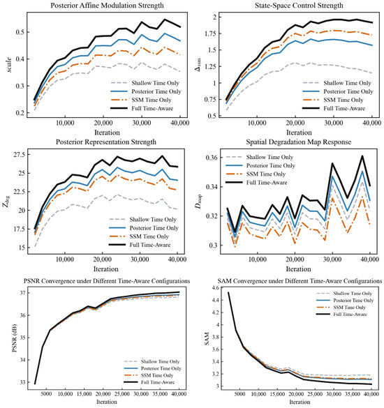
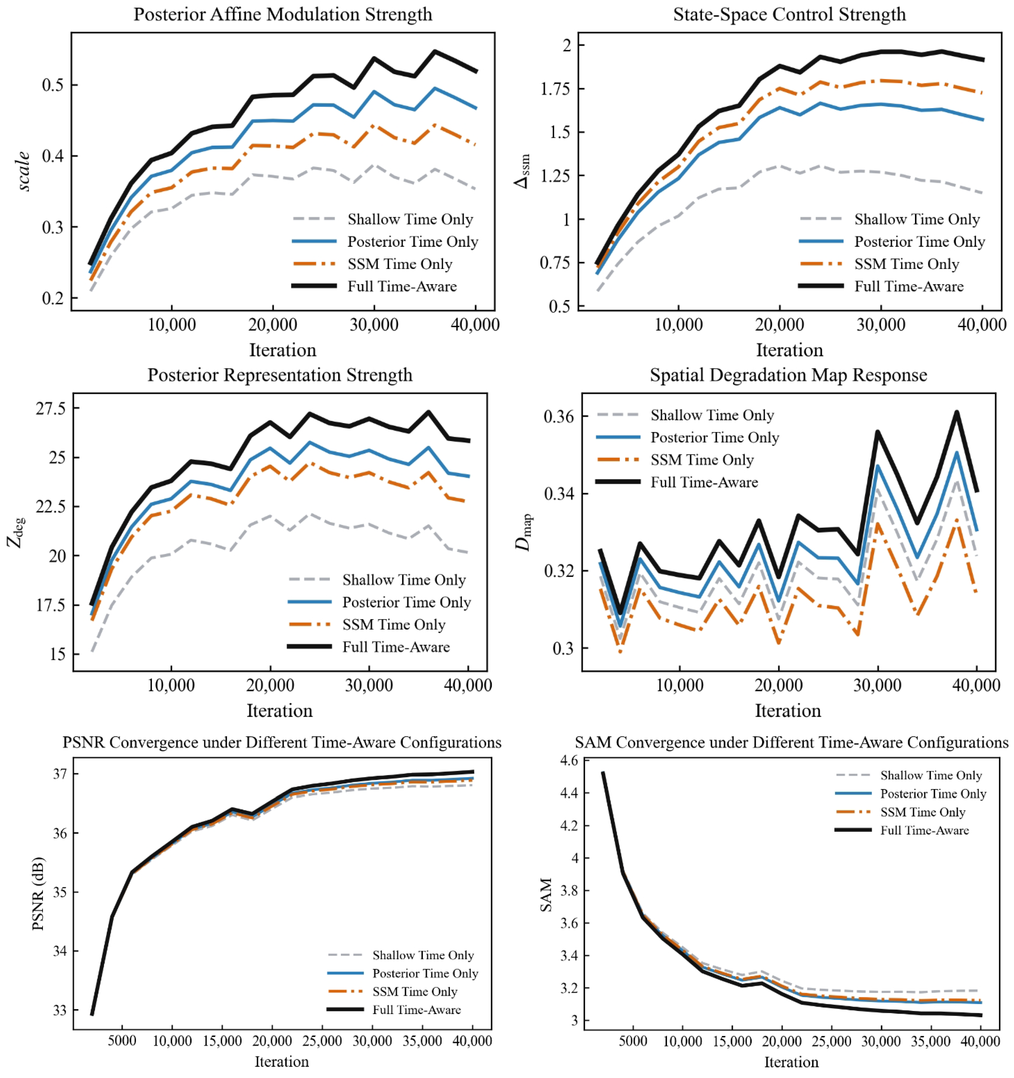
To verify the effectiveness of the time-aware mechanism, we compare four configurations while keeping the remaining network structure and training strategy unchanged: Shallow Time Only, Posterior Time Only, SSM Time Only, and Full Time-Aware. Among them, Shallow Time Only retains only the basic diffusion timestep encoding; Posterior Time Only introduces temporal information only into degradation posterior estimation and posterior control mapping; SSM Time Only performs time modulation only in the state-space main branch; and Full Time-Aware retains deep time injection in both the posterior branch and the main branch.

As shown in Table 9, Shallow Time Only shows the weakest performance, with SAM and PSNR of $3.182$ and $36.804$, respectively. Posterior Time Only and SSM Time Only improve the results to $3.109/36.921$ and $3.123/36.887$, respectively. Full Time-Aware finally achieves the best results of $3.031/37.031$. These results indicate that simple shallow time encoding is insufficient to fully support the denoising process, while temporal injection in the posterior branch and temporal modulation in the main branch both make independent contributions, and their combination achieves the best performance. Combined with the convergence curves and internal state curves shown in Figure 13, it can also be seen that the full time-aware configuration shows more continuous PSNR improvement and SAM reduction during training. Meanwhile, it can more sufficiently establish key control variables such as $\Delta \gamma$, ${\Delta }_{\mathrm{ssm}}$, $scale$, and $shift$. The real training logs also show that the default configuration stably reaches a PSNR level of about 37 dB in the later training stage and reduces SAM to around $0.060$, indicating that the time-aware mechanism not only improves the final performance, but also enhances the establishment of control variables and convergence stability during training.

Table 9. Ablation results of PanDiM under different time-aware mechanisms on the WV3 dataset.

Variant	SAM ↓	PSNR ↑
Shallow Time Only	3.182	36.804
Posterior Time Only	3.109	36.921
SSM Time Only	3.123	36.887
Full Time-Aware	3.031	37.031

Figure 13. Ablation results of different time-aware mechanisms on the WV3 dataset.

4.11. Computational Efficiency Analysis

To further compare the computational efficiency of PanDiM with that of various competing methods, we analyze the trade-off between performance and efficiency in terms of the number of parameters, FLOPs, peak GPU memory, average inference time, FPS, PSNR, and HQNR. The selected comparison methods cover traditional MRA/VO methods, CNN-based methods, Mamba-based methods, diffusion-based methods, and Transformer-based diffusion methods. All statistics are obtained under the same experimental setting, where the batch size is set to 1, the input size is $128\times 128$, the number of multispectral channels is 8, and the number of panchromatic channels is 1, to ensure a fair comparison as much as possible.

As shown in Table 10, traditional methods and some CNN-based methods have relatively low computational costs, but their reconstruction accuracy is limited. Mamba-based methods, such as Pan-Mamba and FusionMamba, exhibit favorable computational efficiency. However, they mainly belong to deterministic reconstruction frameworks and lack the capability of diffusion-based progressive restoration to gradually model complex degradation processes, which still limits their ability to represent fine spatial details.

Table 10. Computational complexity and performance statistics of different representative methods on the WV3 dataset.

Method	Params (M)	FLOPs (G)	GPU Mem. (GB) ↓	Time (s) ↓	FPS ↑	PSNR ↑	HQNR ↑
MTF-GLP-FS	N.A.	N.A.	0.00345	0.00481	208.33	30.921 ± 1.430	0.8698 ± 0.0531
TV	N.A.	N.A.	0.00561	0.0185	54.05	30.542 ± 1.507	0.9187 ± 0.0347
PanNet	0.077640	2.503	0.00852	0.000946	1057.35	33.566 ± 1.841	0.0245 ± 0.0212
Pan-Mamba	0.478	14.042	0.145	0.0262	38.13	32.807 ± 1.643	0.9158 ± 0.0301
FusionMamba	1.105	22.384	0.218	0.0418	23.92	34.293 ± 2.219	0.9304 ± 0.0098
CrossDiff	6.964	9.560	0.0664	0.00886	112.87	35.442 ± 1.350	0.9497 ± 0.0221
PanDiT	392.707	355.173	1.657	0.472	2.12	35.232 ± 2.023	0.9448 ± 0.0185
PanDiM	250.430	292.077	1.128	0.335	2.98	37.031 ± 1.822	0.9574 ± 0.0128

In contrast, diffusion-based methods usually incur higher inference costs due to multi-step denoising sampling. Nevertheless, their denoising generative mechanism helps to more sufficiently model complex spatial details and spectral constraints, often leading to higher-quality reconstruction results, especially in full-resolution experiments. Compared with the Transformer-based diffusion method PanDiT, PanDiM achieves lower computational overhead in all aspects while obtaining higher PSNR and HQNR. Specifically, compared with PanDiT, PanDiM reduces the number of parameters, FLOPs, peak inference memory, and average inference time by approximately 36.2%, 17.8%, 31.9%, and 29.0%, respectively, while improving PSNR and HQNR by approximately 1.799 dB and 0.0126. These results demonstrate that, for high-resolution remote sensing image pansharpening, the diffusion-based Mamba framework can model long-range dependencies through selective state propagation, thereby reducing computational burden while preserving global structural representation capability.

5. Conclusions

We propose PanDiM, a high-fidelity pansharpening framework based on a DiM network. To break through the performance bottleneck of traditional diffusion models in remote sensing image fusion, we reformulate pansharpening as a high-frequency residual restoration process and introduce three key innovations. First, to address the difficulty of existing models in handling complex local degradation, we design DPGM, which converts physical priors into dynamic control variables and gives the state space model spatially adaptive regulation ability, effectively avoiding feature misalignment and local spectral distortion that may be caused by the lack of explicit guidance in traditional methods. Meanwhile, to address the different feature requirements at different denoising stages, we introduce a deeply coupled time-aware mechanism, which allows temporal information to directly participate in feature evolution and gives the model the ability to dynamically adjust its restoration strategy. Finally, for more accurate residual reconstruction, we propose the FDL function, which separates low- and high-frequency components in the frequency domain and applies differentiated constraints, thereby providing precise guidance for high-frequency spatial reconstruction and low-frequency spectral restoration. Experiments on three mainstream benchmark datasets, including WV3, GF2, and QB, show that our model achieves the best results under both reference-based and no-reference evaluations. This study not only significantly improves pansharpening performance, but also provides valuable technical support for high-fidelity image fusion in complex remote sensing scenarios such as waters, ports, and waterways.

References

- Yang, H.; Jiang, Z.; Zhang, Y.; Wu, Y.; Luo, H.; Zhang, P.; Wang, B. A high-resolution remote sensing land use/land cover classification method based on multi-level features adaptation of segment anything model. Int. J. Appl. Earth Obs. Geoinf. 2025, 141, 104659. [Google Scholar] [CrossRef] [Scilit]
- Tang, Y.; Zhang, G.; Liu, J.K.; Qin, R. Weakly supervised land-cover classification of high-resolution images with low-resolution labels through optimized label refinement. Int. J. Remote Sens. 2025, 46, 1913–1937. [Google Scholar] [CrossRef] [Scilit]
- Sun, Y.; Wang, D.; Li, L.; Ning, R.; Yu, S.; Gao, N. Application of remote sensing technology in water quality monitoring: From traditional approaches to artificial intelligence. Water Res. 2024, 267, 122546. [Google Scholar] [CrossRef] [Scilit] [PubMed]
- Jaywant, S.A.; Arif, K.M. Remote sensing techniques for water quality monitoring: A review. Sensors 2024, 24, 8041. [Google Scholar] [CrossRef] [Scilit] [PubMed]
- Kanjir, U.; Greidanus, H.; Oštir, K. Vessel detection and classification from spaceborne optical images: A literature survey. Remote Sens. Environ. 2018, 207, 1–26. [Google Scholar] [CrossRef] [Scilit] [PubMed]
- Baek, W.K.; Kim, E.; Jeon, H.K.; Lee, K.J.; Kim, S.W.; Lee, Y.K.; Ryu, J.H. Monitoring maritime ship characteristics using satellite remote sensing data from different sensors. Ocean Sci. J. 2024, 59, 8. [Google Scholar] [CrossRef] [Scilit]
- Liu, L.; Chu, C.; Chen, C.; Huang, S. MarineYOLO: Innovative deep learning method for small target detection in underwater environments. Alex. Eng. J. 2024, 104, 423–433. [Google Scholar] [CrossRef] [Scilit]
- Vivone, G.; Alparone, L.; Chanussot, J.; Dalla Mura, M.; Garzelli, A.; Licciardi, G.A.; Restaino, R.; Wald, L. A critical comparison among pansharpening algorithms. IEEE Trans. Geosci. Remote Sens. 2014, 53, 2565–2586. [Google Scholar] [CrossRef] [Scilit]
- Zhang, Y.; Zhao, H.; Li, X.; Li, H.; Jin, J. MERS-Net: A lightweight and efficient remote sensing image object detector. IEEE Geosci. Remote Sens. Lett. 2025, 22, 6009005. [Google Scholar] [CrossRef] [Scilit]
- Xu, Q.; Li, B.; Zhang, Y.; Ding, L. High-fidelity component substitution pansharpening by the fitting of substitution data. IEEE Trans. Geosci. Remote Sens. 2014, 52, 7380–7392. [Google Scholar] [CrossRef] [Scilit]
- Aiazzi, B.; Alparone, L.; Baronti, S.; Garzelli, A.; Selva, M. MTF-tailored multiscale fusion of high-resolution MS and Pan imagery. Photogramm. Eng. Remote Sens. 2006, 72, 591–596. [Google Scholar] [CrossRef] [Scilit]
- Meng, X.; Shen, H.; Li, H.; Zhang, L.; Fu, R. Review of the pansharpening methods for remote sensing images based on the idea of meta-analysis: Practical discussion and challenges. Inf. Fusion 2019, 46, 102–113. [Google Scholar] [CrossRef] [Scilit]
- Cui, C.; Liu, L.; Qiao, R. A cutting-edge video anomaly detection method using image quality assessment and attention mechanism-based deep learning. Alex. Eng. J. 2024, 108, 476–485. [Google Scholar] [CrossRef] [Scilit]
- Wang, Z.; Ma, Y.; Zhang, Y. Review of pixel-level remote sensing image fusion based on deep learning. Inf. Fusion 2023, 90, 36–58. [Google Scholar] [CrossRef] [Scilit]
- Cao, Z.; Wu, X.; Deng, L.J.; Zhong, Y. A novel state space model with local enhancement and state sharing for image fusion. In Proceedings of the 32nd ACM International Conference on Multimedia; ACM: New York, NY, USA, 2024; pp. 1235–1244. [Google Scholar]
- Yu, L.; Zhang, D.; Liu, N.; Zhou, W. A multi-view fusion method via tensor learning and gradient descent for image features. IEEE Access 2021, 9, 79389–79399. [Google Scholar] [CrossRef] [Scilit]
- Qian, D.; Yu, L.; Tang, H.; Zhao, J. Multiview feature fusion optimization method for image retrieval based on matrix correlation. J. Electron. Imaging 2020, 29, 053007. [Google Scholar] [CrossRef] [Scilit]
- Liu, Y.; Yue, J.; Xia, S.; Ghamisi, P.; Xie, W.; Fang, L. Diffusion models meet remote sensing: Principles, methods, and perspectives. IEEE Trans. Geosci. Remote Sens. 2024, 62, 4708322. [Google Scholar] [CrossRef] [Scilit]
- Cao, Z.; Cao, S.; Deng, L.J.; Wu, X.; Hou, J.; Vivone, G. Diffusion model with disentangled modulations for sharpening multispectral and hyperspectral images. Inf. Fusion 2024, 104, 102158. [Google Scholar] [CrossRef] [Scilit]
- Fang, J.; Cao, K.; He, X.; Zhang, J.; Zhou, M.; Liu, L. PanDiT: A Few-Step Diffusion Transformer for High-Fidelity and Efficient Pansharpening. IEEE Trans. Geosci. Remote Sens. 2025, 63, 5408413. [Google Scholar] [CrossRef] [Scilit]
- Masi, G.; Cozzolino, D.; Verdoliva, L.; Scarpa, G. Pansharpening by convolutional neural networks. Remote Sens. 2016, 8, 594. [Google Scholar] [CrossRef] [Scilit]
- Yang, J.; Fu, X.; Hu, Y.; Huang, Y.; Ding, X.; Paisley, J. PanNet: A deep network architecture for pan-sharpening. In Proceedings of the IEEE International Conference on Computer Vision; IEEE: Piscataway, NJ, USA, 2017; pp. 5449–5457. [Google Scholar]
- He, L.; Rao, Y.; Li, J.; Chanussot, J.; Plaza, A.; Zhu, J.; Li, B. Pansharpening via detail injection based convolutional neural networks. IEEE J. Sel. Top. Appl. Earth Obs. Remote Sens. 2019, 12, 1188–1204. [Google Scholar] [CrossRef] [Scilit]
- Jin, Z.R.; Zhang, T.J.; Jiang, T.X.; Vivone, G.; Deng, L.J. LAGConv: Local-context adaptive convolution kernels with global harmonic bias for pansharpening. In Proceedings of the AAAI Conference on Artificial Intelligence; AAAI: Palo Alto, CA, USA, 2022; Volume 36, pp. 1113–1121. [Google Scholar]
- Duan, Y.; Wu, X.; Deng, H.; Deng, L.J. Content-adaptive non-local convolution for remote sensing pansharpening. In Proceedings of the IEEE/CVF Conference on Computer Vision and Pattern Recognition; IEEE: Piscataway, NJ, USA, 2024; pp. 27738–27747. [Google Scholar]
- Wang, X.; Zheng, Z.; Shao, J.; Duan, Y.; Deng, L.J. Adaptive rectangular convolution for remote sensing pansharpening. In Proceedings of the Computer Vision and Pattern Recognition Conference; IEEE: Piscataway, NJ, USA, 2025; pp. 17872–17881. [Google Scholar]
- Zhou, M.; Huang, J.; Fang, Y.; Fu, X.; Liu, A. Pan-sharpening with customized transformer and invertible neural network. In Proceedings of the AAAI Conference on Artificial Intelligence; AAAI: Palo Alto, CA, USA, 2022; Volume 36, pp. 3553–3561. [Google Scholar]
- Zhou, H.; Liu, Q.; Wang, Y. PanFormer: A transformer based model for pan-sharpening. In Proceedings of the 2022 IEEE International Conference on Multimedia and Expo (ICME); IEEE: Piscataway, NJ, USA, 2022; pp. 1–6. [Google Scholar]
- Gu, A.; Goel, K.; Ré, C. Efficiently modeling long sequences with structured state spaces. arXiv 2021, arXiv:2111.00396. [Google Scholar]
- Gu, A.; Dao, T. Mamba: Linear-time sequence modeling with selective state spaces. arXiv 2023, arXiv:2312.00752. [Google Scholar]
- Zhu, L.; Liao, B.; Zhang, Q.; Wang, X.; Liu, W.; Wang, X. Vision mamba: Efficient visual representation learning with bidirectional state space model. arXiv 2024, arXiv:2401.09417. [Google Scholar]
- Chen, K.; Chen, B.; Liu, C.; Li, W.; Zou, Z.; Shi, Z. RSMamba: Remote sensing image classification with state space model. IEEE Geosci. Remote Sens. Lett. 2024, 21, 8002605. [Google Scholar] [CrossRef] [Scilit]
- Xiao, Z.; Li, Z.; Cao, J.; Liu, X.; Kong, Y.; Du, Z. OriMamba: Remote sensing oriented object detection with state space models. Int. J. Appl. Earth Obs. Geoinf. 2025, 143, 104731. [Google Scholar] [CrossRef] [Scilit]
- Ma, X.; Zhang, X.; Pun, M.O. RS3mamba: Visual state space model for remote sensing image semantic segmentation. IEEE Geosci. Remote Sens. Lett. 2024, 21, 6011405. [Google Scholar] [CrossRef] [Scilit]
- Liu, Y.; Tian, Y.; Zhao, Y.; Yu, H.; Xie, L.; Wang, Y.; Ye, Q.; Jiao, J.; Liu, Y. Vmamba: Visual state space model. Adv. Neural Inf. Process. Syst. 2024, 37, 103031–103063. [Google Scholar] [CrossRef] [Scilit]
- Hu, V.T.; Baumann, S.A.; Gui, M.; Grebenkova, O.; Ma, P.; Fischer, J.; Ommer, B. Zigma: A dit-style zigzag mamba diffusion model. In Proceedings of the European Conference on Computer Vision; Springer: Berlin/Heidelberg, Germany, 2024; pp. 148–166. [Google Scholar]
- He, X.; Cao, K.; Zhang, J.; Yan, K.; Wang, Y.; Li, R.; Xie, C.; Hong, D.; Zhou, M. Pan-mamba: Effective pan-sharpening with state space model. Inf. Fusion 2025, 115, 102779. [Google Scholar] [CrossRef] [Scilit]
- Peng, S.; Zhu, X.; Deng, H.; Deng, L.J.; Lei, Z. Fusionmamba: Efficient remote sensing image fusion with state space model. IEEE Trans. Geosci. Remote Sens. 2024, 62, 5410216. [Google Scholar] [CrossRef] [Scilit]
- Croitoru, F.A.; Hondru, V.; Ionescu, R.T.; Shah, M. Diffusion models in vision: A survey. IEEE Trans. Pattern Anal. Mach. Intell. 2023, 45, 10850–10869. [Google Scholar] [CrossRef] [Scilit] [PubMed]
- Tian, C.; Chen, Y. Image segmentation and denoising algorithm based on partial differential equations. IEEE Sens. J. 2019, 20, 11935–11942. [Google Scholar] [CrossRef] [Scilit]
- Ho, J.; Jain, A.; Abbeel, P. Denoising diffusion probabilistic models. Adv. Neural Inf. Process. Syst. 2020, 33, 6840–6851. [Google Scholar]
- Song, J.; Meng, C.; Ermon, S. Denoising diffusion implicit models. arXiv 2020, arXiv:2010.02502. [Google Scholar]
- Kawar, B.; Elad, M.; Ermon, S.; Song, J. Denoising diffusion restoration models. Adv. Neural Inf. Process. Syst. 2022, 35, 23593–23606. [Google Scholar] [CrossRef] [Scilit]
- Peebles, W.; Xie, S. Scalable diffusion models with transformers. In Proceedings of the IEEE/CVF International Conference on Computer Vision; IEEE: Piscataway, NJ, USA, 2023; pp. 4195–4205. [Google Scholar]
- Teng, Y.; Wu, Y.; Shi, H.; Ning, X.; Dai, G.; Wang, Y.; Li, Z.; Liu, X. Dim: Diffusion mamba for efficient high-resolution image synthesis. arXiv 2024, arXiv:2405.14224. [Google Scholar]
- Xing, Y.; Qu, L.; Zhang, S.; Zhang, K.; Zhang, Y.; Bruzzone, L. Crossdiff: Exploring self-supervisedrepresentation of pansharpening via cross-predictive diffusion model. IEEE Trans. Image Process. 2024, 33, 5496–5509. [Google Scholar] [CrossRef] [Scilit] [PubMed]
- Bao, F.; Nie, S.; Xue, K.; Cao, Y.; Li, C.; Su, H.; Zhu, J. All are worth words: A vit backbone for diffusion models. In Proceedings of the IEEE/CVF Conference on Computer Vision and Pattern Recognition; IEEE: Piscataway, NJ, USA, 2023; pp. 22669–22679. [Google Scholar]
- Deng, L.J.; Vivone, G.; Paoletti, M.E.; Scarpa, G.; He, J.; Zhang, Y.; Chanussot, J.; Plaza, A. Machine learning in pansharpening: A benchmark, from shallow to deep networks. IEEE Geosci. Remote Sens. Mag. 2022, 10, 279–315. [Google Scholar] [CrossRef] [Scilit]
- Wald, L.; Ranchin, T.; Mangolini, M. Fusion of satellite images of different spatial resolutions: Assessing the quality of resulting images. Photogramm. Eng. Remote Sens. 1997, 63, 691–699. [Google Scholar]
- Vivone, G.; Dalla Mura, M.; Garzelli, A.; Restaino, R.; Scarpa, G.; Ulfarsson, M.O.; Alparone, L.; Chanussot, J. A new benchmark based on recent advances in multispectral pansharpening: Revisiting pansharpening with classical and emerging pansharpening methods. IEEE Geosci. Remote Sens. Mag. 2020, 9, 53–81. [Google Scholar] [CrossRef] [Scilit]
- Vivone, G.; Restaino, R.; Chanussot, J. Full scale regression-based injection coefficients for panchromatic sharpening. IEEE Trans. Image Process. 2018, 27, 3418–3431. [Google Scholar] [CrossRef] [Scilit] [PubMed]
- Palsson, F.; Sveinsson, J.R.; Ulfarsson, M.O. A new pansharpening algorithm based on total variation. IEEE Geosci. Remote Sens. Lett. 2013, 11, 318–322. [Google Scholar] [CrossRef] [Scilit]
- Vivone, G. Robust band-dependent spatial-detail approaches for panchromatic sharpening. IEEE Trans. Geosci. Remote Sens. 2019, 57, 6421–6433. [Google Scholar] [CrossRef] [Scilit]
- Fu, X.; Lin, Z.; Huang, Y.; Ding, X. A variational pan-sharpening with local gradient constraints. In Proceedings of the IEEE/CVF Conference on Computer Vision and Pattern Recognition; IEEE: Piscataway, NJ, USA, 2019; pp. 10265–10274. [Google Scholar]
- Wu, Z.C.; Huang, T.Z.; Deng, L.J.; Huang, J.; Chanussot, J.; Vivone, G. LRTCFPan: Low-rank tensor completion based framework for pansharpening. IEEE Trans. Image Process. 2023, 32, 1640–1655. [Google Scholar] [CrossRef] [Scilit] [PubMed]
- Deng, L.J.; Vivone, G.; Jin, C.; Chanussot, J. Detail injection-based deep convolutional neural networks for pansharpening. IEEE Trans. Geosci. Remote Sens. 2020, 59, 6995–7010. [Google Scholar] [CrossRef] [Scilit]
- Wu, X.; Huang, T.Z.; Deng, L.J.; Zhang, T.J. Dynamic cross feature fusion for remote sensing pansharpening. In Proceedings of the IEEE/CVF International Conference on Computer Vision; IEEE: Piscataway, NJ, USA, 2021; pp. 14687–14696. [Google Scholar]
- Tian, X.; Li, K.; Zhang, W.; Wang, Z.; Ma, J. Interpretable model-driven deep network for hyperspectral, multispectral, and panchromatic image fusion. IEEE Trans. Neural Netw. Learn. Syst. 2023, 35, 14382–14395. [Google Scholar] [CrossRef] [Scilit]
- Shu, W.J.; Dou, H.X.; Wen, R.; Wu, X.; Deng, L.J. CMT: Cross modulation transformer with hybrid loss for pansharpening. IEEE Geosci. Remote Sens. Lett. 2024, 21, 5004405. [Google Scholar] [CrossRef] [Scilit]
Disclaimer/Publisher’s Note: The statements, opinions and data contained in all publications are solely those of the individual author(s) and contributor(s) and not of MDPI and/or the editor(s). MDPI and/or the editor(s) disclaim responsibility for any injury to people or property resulting from any ideas, methods, instructions or products referred to in the content. |
© 2026 by the authors. Licensee MDPI, Basel, Switzerland. This article is an open access article distributed under the terms and conditions of the Creative Commons Attribution (CC BY) license.